Automatic Conversion of Meshes to T-spline Surfaces

Category: Research

Abstract

We give anautomaticmethod for fitting T-spline surfaces to trian-gle meshes of arbitrary topology. Previous surface fitting methodsrequired tedious human interaction to accurately capture the geom-etry and features. There are two main steps in our method. Thefirst computes a curvilinear coordinate system—aconformal net—on the surface, induced by global conformal parameterization. Thisglobal net is then automatically partitioned to give several rectan-gular patches which locally have tensor product structure suitablefor defining splines. In the second step, each rectangular patch isapproximated to a desired positional and normal accuracy bya T-spline surface, with appropriate continuity between patchbound-aries. Use of T-splines enables us to use a low number of controlpoints while guaranteeingL∞ error behaviour. The only user inputsrequired in the whole process are these two fitting tolerances.

CR Categories: I.3.5 [Computational Geometry and Object Mod-eling]: Splines—T-Splines; I.3.5 [Computational Geometry andObject Modeling]: Boundary Representations—Mesh;

Keywords: Polygonal meshes, Spline surfaces, Riemann surfaces,Global conformal parameterization, T-splines

1 Introduction

Triangle meshes and spline surfaces are the most widely usedrepre-sentations in computer graphics and geometric modelling. Trianglemeshes are supported by graphics hardware and hence are widelyused for visualization, computer games, etc. Spline surfaces arethe main representation used for computer aided design and manu-facturing. Using 3D laser scanners, surface data from real objectscan easily be acquired [Bernardini and Rushmeier 2002]. This isusually initially in the form of unorganized points, which are thenjoined to form a triangular mesh. In order to use these meshesinmany current CAD systems, and to facilitate interactive editing, itis necessary to convert them to spline surfaces. Furthermore, alter-native representations are more suited to different applications, soautomatic conversion between them is of great importance.

NURBS surfaces are of widespread use, but they have severaldisadvantages. Recently, Sederberg et al. generalized them, givingT-splines [Sederberg et al. 2003; Sederberg et al. 2004]. T-splinesrequire significantlyfewercontrol points to represent complex ge-ometric information: they have better local refinement capabilities,because of the more flexible approach to joining T-splines attheircommon boundaries.

Traditional surface fitting methods minimize global errorsin aleast squares sense, and do not ensure a boundedL∞ error norm,which may be required by users. The local refinement method ofT-splines makes them well suited to mesh fitting, where an adaptivealgorithm can locally achieve the desired approximation quality andcontrolL∞ errors. The quality of normal vectors of the fitted surface

is also often important. Our approach combines positional and nor-mal tolerances in the objective function used for fitting, allowing usto bound both kinds of error.

To convert meshes of arbitrary topology to parametric surfaces,including T-splines, they must first be parameterized. We use con-formal parameterization, which preserves angles between the pa-rameterization and the surface, ensuring that the parameterization iswell behaved, thus helping to guarantee high-quality reconstructednormals. Because T-splines areglobally defined on meshes, we donot wish to partition the mesh into many separately parameterizedpatches: instead, we use a global parameterization:global confor-mal parameterization, introduced in [Gu and Yau 2003].

The latter works by finding a smooth pair of vector fields mutu-ally orthogonal to each other except at a number ofzero points; asurface of genusg has|2g−2| zero points. The two families of inte-gral curves of these fields are arbitrarily calledhorizontalandverti-cal trajectories, and form aconformal net. Locally, this has a tensorproduct structure, enabling knots of a T-spline to be defineddirectlyon it. Globally, conformal nets have a particular structurewhich canbe directly used for T-spline fitting: horizontal trajectories throughthe zero points segment the mesh into topological cylindersanddisks. Each segment can be mapped to a planar rectangle by map-ping the horizontal and vertical trajectories to iso-parametric linesin the plane. T-spline patches can be defined on these rectanglesdirectly. By using common knots and control points along theirboundaries, the desired continuity can be achieved.

Novelty This work presents an automatic algorithm for convert-ing triangle meshes to T-Spline surfaces, requiring only a user-specifiedL∞ position tolerance and a normal tolerances. It workssurfaces with multiple handles and open boundaries. The algorithmis based on the intrinsic Riemann structure of the surface, which isindependent of the triangulation: it is stable with respectto smalldeformations. The parameter net of the T-spline surface is close toconformal, which is valuable for purposes of texture mapping andgeometric computation.

2 Related work

Before presenting our new method, we discuss related work intwoareas: fitting methods, and global parameterization methods.

2.1 L2 surface fitting

Surface fitting techniques can be classified asapproximatingtech-niques andinterpolationtechniques.

Finding a parametric surfaceSwhich approximates a target sur-faceT is usually performed by minimizing the distance betweenthem with respect to some metric. The distance metric usually usedis a weighted sum of squared distances of samplesti taken fromTto S:

L2(T,S) = ∑ti∈T

wi‖d(ti ,S)‖2. (1)

Here,d(t,S) denotes the distance betweent and its image pointsonS: d(t,S) = ‖t −s‖. Weights typically reflect the sampling density,which may not be uniform. Finding the image points is a key stepin fitting, and can be done in two basic ways, with or without theaid of a parameterization.

1

Parameterization-free methods find image points by computingfoot points of the samples on the approximating surface withre-spect to Euclidean distance. Much work has been done on thisproblem. A survey is given in [Sapidis 1994]; for more recentadvances, see [Dodgson et al. 2003; Marinov and Kobbelt 2004].Parameterization-based methods parameterize the target surface ina planar domain, and then select the image points by identifyingthe parameter values. Such methods have also received consider-able attention; an extensive survey is given in [Weiss et al.2002].

Both of these approaches are limited. In parameterization-freemethods, nearest point computation is time-consuming and errorprone [Marinov and Kobbelt 2004]. Selecting a good initial surfacefor iterative optimization is also difficult [Cheng et al. 2004]—self-intersection of the control mesh can easily result if the curvatureof the target surface changes rapidly. To avoid this problem, a sur-face fairness term is usually added, but choosing the best balancesmoothness and a good fit is tricky [Weiss et al. 2002].

Parameterization-based methods either rely on minimizingaglobal error function, or projecting samples projected onto abasesurface, which can again be hard to choose. Both approaches canintroduce serious local distortions, resulting in unwanted ripples forcomplicated surfaces.

Irregular distribution of data points on the target surfaceis an-other serious problem for surface approximation techniques. Tocircumvent this issue, Pottmann et.al [Pottmann and Leopoldseder2003] devised an approach in which the roles ofT and S areswapped. One can compute the distance field forSas a prior, by-passing the problem of irregularly spaced data points. However,their approach still suffers from the other problems associated withnearest point methods and is not well suited to approximating com-plicated surfaces.

Interpolation schemes are an alternative to approximation. Usu-ally, a set of interpolation constraints [Halstead et al. 1993] is gener-ated, and fitting is performed by solving a linear system. However,this approach can suffer from poor conditioning. Litke et al. [Litkeet al. 2001] introduced a quasi-interpolation scheme in which thecontrol points are computed from the target surface directly. Inter-polation schemes suffer from two problems. Again, like approxi-mation schemes, they need a parameterization; choosing theinter-polation constraints is also hard.

2.2 L∞ surface fitting

Surface fitting using a fixed number of control points can not guar-antee high approximation quality. To obtain boundedL∞ fittingerrors, additional control points need to be inserted as fitting pro-ceeds, to accommodate local shape details.

Multiresolution structures have been used in [Lee et al. 2000;Litke et al. 2001] as a means of reducing theL∞ error adaptively.Although this approach can produce high approximation quality,the usual approach subdivides the surfaceglobally, making manyof the added control points redundant.

Instead, if we try to refine the surface locally, and insert knotswhere the approximation error is high, we have the difficult issueof deciding how many knots should be inserted. A common ap-proach [Cham and Cipolla 1999; Yang et al. 2004] inserts knots intothe region of maximumL∞ error and then does global optimization.This strategy works well for curve fitting, but for surface fitting,simply subdividing the region having maximumL∞ error does notwork well in practice. Marinov et al. [Marinov and Kobbelt 2004]suggest inserting knots intoall regions where theL∞ error exceeds agiven threshold. However, this has the disadvantage of introducingredundant control points that need to be subsequently removed.

By using T-splines, we are able locally insert knots, and onlyhave to perform local fitting to adjust the surface, without an ex-pensive global computation—the surface elsewhere remainsun-changed.

2.3 Segmentation methods

To fit a parametric surface to a polygon mesh of arbitrary topology,the polygon mesh is usually segmented into a number of rectan-gular regions that are approximated by parametric patches.Manyprevious methods, e.g. [Andersson et al. 1988; Krishnamurthy andLevoy 1996], require the user to manually delineate the patchboundaries. However, for surfaces of complicated topology, thisis very tedious.

Instead of using manual interaction, Eck and Hoppe [Eck andHoppe 1996] describe a method for producing quadrilateral patchesbased on a parameterization phase [Eck et al. 1995] and a remesh-ing phase. The number of patches is adjusted to achieve desired fit-ting tolerances. While this method produces high quality surfaces,many extra control points are needed to achieve continuity alongboundaries and at patch corners.

Katz et al [Katz and Tal 2003] give another mesh segmentationapproach based on fuzzy clustering and cuts. Their method, whileuseful, produces segments which do not always have rectangularboundaries. Also, further parametrization is needed to ensure con-tinuity along boundary curves.

We use global conformal parameterization as a means of pro-viding automatic segmentation; it also gives the parameterizationneeded for T-spline fitting, guaranteeing continuity alongpatchboundaries.

2.4 Conformal parameterization

Several recent advances in surface parameterization [Floater andHorman 2004] have been based on solving a discrete Laplace sys-tem [Pinkall and Polthier 1993; Duchamp et al. 1997; Floater1997;Floater 2003]. Levy et al. [Levy et al. 2002] describe a techniquefor finding conformal mappings by least squares minimization ofconformal energy, and Desbrun et al. [Desbrun et al. 2002] for-mulate a theoretically equivalent method of discrete conformal pa-rameterization. Sheffer et al. [Sheffer and Sturler 2001] give anangle-based flattening method for conformal parameterization.

Gu and Yau [Gu and Yau 2003] considered construction of aglobal conformal structure for a manifold of arbitrary topology byfinding a basis for holomorphic differential forms, based onHodgetheory [Schoen and Yau 1997].

Ni et al. [Ni et al. 2004] use the idea of a harmonic Morsefunction to extract the topological structure of a surface.Dong etal. [Dong et al. 2005, to appear] give a method for quadrilateralremeshing of manifolds using harmonic functions. The method istheoretically equivalent to using a holomorphic differential form asdescribed in [Gu and Yau 2003]. The differential forms in thelatterhave at least 4 fewer zero points than those in the former, however.For the current problem, it is desirable to have fewer zero points, asthey affect the global structure of the parameterization significantly.Thus, we have adapted Gu and Yau’s method. Note, however, thatwe do not remesh the surface, but fit a spline on the parameter do-main directly.

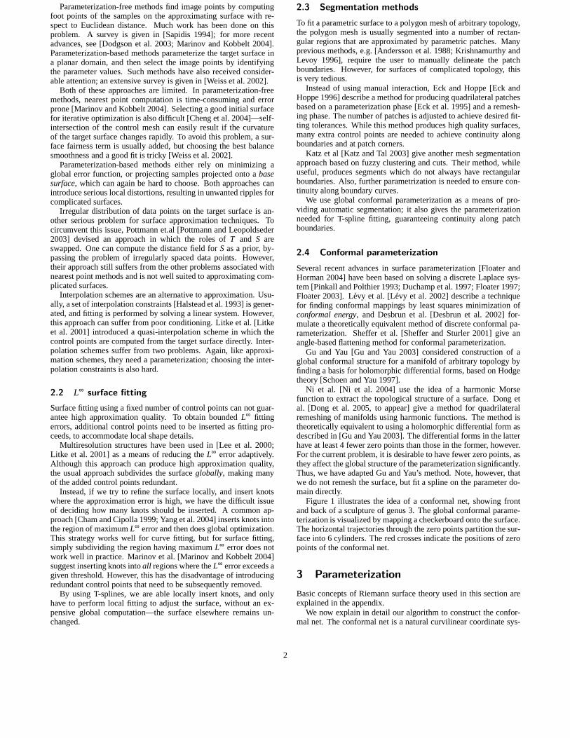
Figure 1 illustrates the idea of a conformal net, showing frontand back of a sculpture of genus 3. The global conformal parame-terization is visualized by mapping a checkerboard onto thesurface.The horizontal trajectories through the zero points partition the sur-face into 6 cylinders. The red crosses indicate the positions of zeropoints of the conformal net.

3 Parameterization

Basic concepts of Riemann surface theory used in this section areexplained in the appendix.

We now explain in detail our algorithm to construct the confor-mal net. The conformal net is a natural curvilinear coordinate sys-

2

Figure 1: Global conformal parameterizationtem on A surface. Locally, conformal nets have a tensor productstructure, so are suitable for defining a T-spline surface. They alsohave a simple global structure: they can be treated as rectangleswith regular grids, glued along their edges and at zero points in aspecial pattern—see Figure 2. Figure 2(a) illustrates fourregularrectangles; the black dots are the zero points. Figure 2(b) showshow each rectangle is mapped to a quadrant, and merged togetherat the zero point. Figure 2(c) shows three at a central zero point.The red curves are the horizontal trajectories, and the blueones

Figure 2: Global structure of conformal nets.

are the vertical trajectories. Note that in the general case, exactlyfour patches meet at a zero point, and each rectangle is mappedto a quadrant. Gluing opposite sides of a single rectangle gives acylinder or a torus.

The input surface is represented by a triangular mesh, and eachvector field is represented as a function defined on the edges of themesh.

SupposeK is a simplicial complex, and a mappingr : K → R3

embedsK in R3. ThenM = (K, f ) is called atriangular mesh. Fordimensionsn = 0,1,2, we denote the sets ofn-simplicesby Kn.Any given n-simplex is denoted by[v0,v1, · · · ,vn], wherevi ∈ K0,i.e. thevi are points. A holomorphic 1-form is represented as afunction defined on the edges:ω : K1 → R2.

The methods for constructing a conformal net vary differenttypes of surface. We now explain the details for each case: genus-0closed surfaces, genus-1 closed surfaces, higher genus closed sur-faces and surfaces with boundaries.

3.1 Genus-0 closed surfaces

Every genus zero closed surfaceScan be conformally mapped to asphere. Practical algorithms for computing such maps are givenin [Gu et al. 2004; C. Gotsman 2003]. The idea used in [Guet al. 2004] is that, for genus-0 closed surfaces, conformalmapsare equivalent to harmonic maps, which can be computed usingtheheat flow method.

Having found the conformal mapf : S→S2 to the sphere, we usespherical coordinates(θ ,φ) as parameters. The horizontal trajec-tories onSare the curvesf−1(φ = const.), and the vertical trajec-tories aref−1(θ = const.). The preimages of the North and Southpoles are the zero points. The trajectories are orthogonal every-where except at the zero points and form the conformal net.

3.2 Genus-1 closed surfaces

In this case, to find the conformal net, we need to first computea holomorphic 1-formω which can be treated as a pair of vectorfieldsω = (ωu,ωv) satisyingωv = n×ωu, wheren is the surfacenormal. Furthermore,ωu andωv should be harmonic (informaly,they should be as smooth as possible). The horizontal trajectoriesare the integral curves ofωu, the vertical trajectories are the integralcurves ofωv.

For a surface of genusg, all holomorphic 1-forms form a real2g dimensional linear space. Algorithms for finding a holomorphic1-form basis are given in [Gu and Yau 2003], which can be summa-rized as computing in turn a homology basis, a cohomology basis,a harmonic 1-form basis and a holomorphic 1-form basis. It isbe-yond the scope of the current paper details this further. See[Gu andYau 2003] for thoroughly explanations.

In our implementation, the holomorphic 1-form basis{ω1,ω2, · · · ,ω2g} is represented by vector-valued functionsdefined on the edges of the mesh,ωi : K1 → R2, i = 1,2, · · · ,2g.Any discrete holomorphic one-formω is a linear combination ofthem. There are an infinite number of holomorphic 1-forms onS;we want to choose the best one for the purposes of spline fitting.

Each holomorphic 1-formω induces a parameterization ofS. Wecan choose a topological diskU onS, an arbitrary pointp∈U , anddefine the parameterizationz : U → R2, for any pointq∈U , using

z(q) =

∫ q

pω = (

∫ q

pωu,

∫ q

pωv), (2)

where the path fromp to q is arbitrary as long as it lies insideU .For the mesh,U is a set of neighboring triangles, andp andq

are vertices. The path connectingp to q is a series of consecutiveedges, and denoted by{e1,e2, · · · ,en}. The parameter of vertexq iscomputed by the discrete sum

z(q) =n

∑i=1

ω(ei). (3)

Under a conformal parameterization{U,z}, z= (u,v), the metriconScan be represented in the simple form

ds2 = λ 2(u,v)(du2 +dv2), (4)

whereλ (u,v)—the conformal factor–measures area stretching ofthe parameterization. The uniformity of the parameterization canbe measured by computing

E(ω) =∫

U|∇λ |2dudv. (5)

We select the holomorphic 1-form which minimizes this unifor-mity functional, using an automatic algorithm in [Jin et al.2004].

A holomorphic 1-formω on a genus-1 closed surfaceS isnonzero everywhere, so there are no zero points, and the confor-mal net is simple. By integratingω on S, the whole surface canbe conformally mapped to a parallelogram on the plane, called thefundamental periodof S. In general, this is not a rectangle, but askewed parallelogram whose shape is determined by the conformalstructure ofS. If the fundamental period is a rectangle, then all thehorizontal and vertical trajectories forming the conformal net onthe surface are closed circles. Otherwise, we two families of curvesparallel to the sides of the parallelogram are used as the trajectories.

3.3 Higher genus closed surfaces

The global structure of conformal nets on higher genus closed sur-faces is more complicated due to the existence of zero points. Bythe Poincare-Hopf theorem, every vector field on a surface of genus

3

g > 1 must have zero points. A holomorphic 1-form has the uniqueproperty that it has the minimal number of zero points, whichfor asurface of genusg is |2g−2|.

A horizontal trajectory starting from a zero point also endsat azero point. In general there are four horizontal trajectories startingat each zero point. These trajectories partition the surface into sev-eral patches, each of which is either a topological cylinderor disk.By integratingω on each patch using Eqns. 2,3, each patch can beconformally mapped to a rectangle. The resulting conformalnet oneach patch has a regular tensor product structure.

Using this, the conformal net of a higher genus closed surfacecan be constructed using the following steps: (i) Define a regu-lar tensor product grid structure on each rectangle. (ii) Glue pairsof opposite sides of each rectangle to form a cylinder. (iii)Gluethe various rectangles and cylinders along their boundaries as de-termined by the conformal structure and the selected holomorphic1-form.

In order to partition the conformal net into rectangles, we firstneed to locate the|2g− 2| zero points, then trace the horizontaltrajectories through them.

Locating zero points Suppose we have computed a holomor-phic 1-formω. We first estimate the inverse of theconformal factor(see Eqn. 4) for each vertexv of the input surface mesh, using thefollowing formula:

τ(v) = λ−1(v) =1n ∑

[u,v]∈K1

|ω([u,v])|2

|r(u)− r(v)|2, u,v∈ K0, (6)

whereu runs over all vertices connected by an edge tov, r(u) is theposition of vertexu, [u,v] represents an edge fromu to v, ω([u,v])is the value ofω on edge[u,v], andn is the valence of vertexv. Atzero points,λ approaches zero.

We select clusters of vertices whose conformal factors havethelowest 5% of values as candidate locations for zero points. We mea-sure the geometric size of each cluster by computing its diameter,sort them by decreasing size and keep the first|2g−2| clusters. Foreach cluster, we select the vertex closest to the center of gravity ofthe cluster as the zero point associated with that cluster.

Tracing horizontal trajectories through zero points Next,each of the four horizontal trajectories through each zero pointneeds to be found.

Supposep is a zero point. We select an open setU on the mesharoundp: a collection of neighboring faces forming a topologicaldisk. Let the boundary ofU be∂U . We parameterizeU by integrat-ing ω as described in Eqns. 2,3. We denote the parameterization byz : U → R2, z(q) = (z1(q),z2(q)) =

∫ qp ω. Let the horizontal trajec-

tory throughp beγ ; γ is mapped to thex-axis of the plane.We next find all edges[u,v], such thatz([u,v]) intersects thex-

axis, i.e. for whichz2(u) · z2(v) < 0, and we split each edge[u,v]by adding a new vertex atr(w) with parameterz(w):

r(w) = αr(v)+(1−α)r(u), z(w) = αz(v)+(1−α)z(u), (7)

whereα = z2(u)/(z2(u)− z2(v)). We now connect all newly in-serted vertices to form the horizontal line in the plane and the hori-zontal trajectory on the mesh accordingly. We will find four curveswhich are part of the horizontal trajectoryγ .

Next, we select another open setU ′ on the mesh, overlappingwith U , to be the next chart. We parameterizeU ′ in a similar way byintegratingω on it, givingz′ :U ′ →R2. The image ofγ , z′(γ), is stilla horizontal line. We select one of the inserted verticesw∈U ∩U ′;the liney = z′2(w) is z′(r). Using the same approach as for findingγ in U , we can extendγ onU ′ accordingly. In this way we extendγchart by chart, until reaching another zero point.

Ultimately, all the horizontal trajectories through zero points par-tition the surface into several patches, each of which is either atopological cylinder or a disk. If it is a cylinder, we pick anar-bitrary point on it, and trace the corresponding vertical trajectorythrough the point to slice it into a disk. Then all disks are confor-mally parameterized by a rectangle usingω.

3.4 Surfaces with boundaries

For surfaces with boundaries, computing a conformal net needs afurther step:double covering.

Given a surfaceSwith boundaries∂S, we replicate it, and reversethe orientation of the copy,−S, by reversing the vertex order aroundeach face. We glueS to −S along corresponding boundaries: if∂S= σ1∪σ2 · · · ∪σk, then∂ −S= −σ1 ∪−σ2 · · · ∪−σk, andσiis glued to−σi . The double covered surface is a closed surfaceS.Each face ofShas two copies onS.

If S is a topological sphere, we can conformally map it to asphere using a special conformal map which maps the boundaryof S to the equator. The preimages of the lines of longitude andlatitude form the conformal net.

More generally, ifShas genusg andb boundaries,S is a closedsurface with genus 2g+ b− 1. We compute the holomorphic 1-form basis ofS, and then find a special holomorphic 1-formω =(ωu,ωv) on it such thatωu is orthogonal to∂S everywhere, usingthe approach in [Gu and Yau 2003]. Thisω induces a conformalnet onS itself for which all curves in∂S are vertical trajectories.The algorithm for locating zero points is similar to that forclosedsurfaces, except that in the tracing algorithm, horizontaltrajectoriesstarting from zero points may end at the boundary.

3.5 Mesh thinning

Computing the global conformal parametrization for a trianglemesh needs the solution of a linear system, which is expensive fora large number of vertices. We use this parameterisation to give thesegmentation, and the topology of the initial T-spline. Forthis, wedo not need a precise conformal parameter for every vertex oftheinput mesh. Thus, for speed, we simply the intial mesh using Gar-land’s method [Garland and Heckbert 1997] and before computingthe global conformal parametrization.

4 T-splines

This section briefly reviews T-splines and their properties[Seder-berg et al. 2003; Sederberg et al. 2004]. T-spline surfaces are ageneralization of B-spline surfaces.

The control mesh for a T-spline surface is called a T-mesh.Figure 3 shows a pre-image of a T-mesh: it is a rectangular grid

Figure 3: Pre-image of a T-mesh

allowing T-junctions. Each edge is a line segment along theu or vdirection. A T-junction is a vertex shared by oneu-edge and two

4

v-edges, or vice versa. Each edge in a T-mesh is associated with aknot interval, constrained by the following rules:Rule 1: The sum of the knot intervals on opposing edges of anyface must be equal. �

Rule 2: If two T-junctions on opposing edges of a face can be con-nected without violating the previous rule, that edge must be in-cluded in the T-mesh. �

If a T-mesh does not contain any T-junctions, the correspondingT-spline degenerates to a B-spline surface.

The knot information is used to represent a T-spline surface:

P(u,v) =N

∑i=1

wiPiBi(u,v)/N

∑i=1

wiBi(u,v), (8)

wherePi = (xi ,yi ,zi) are theN control points inR3 with associatedweightswi , andBi(u,v) are blending functions defined in terms ofcubic B-spline basis functions:

Bi(u,v) = N[ui0,ui1,ui2,ui3,ui4](u)N[vi0,vi1,vi2,vi3,vi4](v). (9)

The knot vectors ui = [ui0,ui1,ui2,ui3,ui4] andvi = [vi0,vi1,vi2,vi3,vi4] are determined as follows:Rule 3: Let (ui2,vi2) be the knot coordinates ofPi. Consider a rayin parameter spaceR(α) = (ui2 +α,vi2). Starting atPi , ui3 andui4are theu coordinates of the first twou-edges intersected by the raygoing in the+α direction, andui1 andui0 in the opposite direction.Thev knots are found likewise. �

For example, in Figure 3, considerP1 with knot valueu1. Followinga horizontal ray, we hit edges to the left giving knot values of u1−d1 − d2 −d3 andu1 − d3, and to the right, knot values ofu1 + d4andu1 +d4 +d5.

5 Surface fitting

We now consider how to find the optimal collection of T-splinesminimizing the distance between the fitted surface and the triangu-lar mesh, while capturing the geometric shape.

After creating an initial approximate T-spline surface, wecarryout global and local optimization steps. The local steps areaimedat minimizing theL∞ errors for positions and normals by local ad-justment, while global optimization is used to ensure appropriatepositioning of the control points overall and to remove unwantedripples generated during the local approximation process.

Finding a good balance between global and local optimizationis essential for achieving high quality surface; we use an automaticstrategy to do so. Between two successive global approximationphases, several phases of local optimization are performed, duringwhich any one face of the T-mesh may only be subdivided once.Faces generated in the local approximation phases are flagged, andif any face is to be subdivided again, we switch from local approx-imation back to global approximation. These two processes areiterated until the desired tolerance is reached after a global approx-imation step.

We now consider these steps in detail

5.1 Initial T-spline surface

Segmentation splits the simplified mesh into several rectangularpatches. We define a T-spline over each patch such that continu-ity is preserved along their common boundary curves.

The initial T-splines are constructed in two steps. A topologystep determines the structure of the T-mesh for each T-spline. Oncethe required knots for each T-mesh have been specified, a geometrystep computes the Cartesian coordinates of each knot. Weights ofcontrol points in the initial T-splines are set to 1.

In the topology step, for each T-mesh, interior knots and bound-ary knots are distributed separately. Using the conformal param-eterization, interior knots are distributed on a uniform rectangulargrid. Boundary knots are distributed to preserve continuity alongboundary curves and points. At ordinary boundary points andT-junctions, we follow the usual T-spline approach.C2 continuity isobtained at such points as they locally form a T-mesh. Boundarypoints arising near double covering fold points and zero points aretreated specially. See 4, left (before and after folding) and right,respectively. Certain control points around these points are con-strained to lie in the same plane. The red point is the point inques-tion, and the black points show the surrounding knots which areconstrained. This enforcesG1 continuity at these locations.

Figure 4: Knots near double covering fold points and zero points.

The geometry step is then posed as a constrained least-squaresminimization problem. Under the continuity constraints mentionedabove, we minimize the sum of squared distances between ver-tices in the simplified mesh and their images in the initial T-splinesat the corresponding parameter values. The objective function isquadratic and the constraints linear, leading to a linear system.

5.2 Notation

Before discussing global and local approximation, we give the no-tation used. LetV = {v1, . . . ,vm} andF = { f1, . . . , fn} denote thesets of vertices and faces of the input meshM. We use(uvi ,vvi )to denote the conformal parameters,nvi , the normal direction, andvu

i ,vvi , the first-order derivatives of the discrete mesh in theu and

v directions.S= {Si} is the piecewise approximating T-spline sur-face andT = {Ti} is its T-mesh. The T-spline cells are collectedin C = {Cj}. Certain samples are selected from each cellCj , asexplained later; let them be denoted byp jk. The conformal param-eters and their image points on the input meshM are denoted by(u jk,v jk) andq jk respectively.

5.3 Global approximation

In this phase, we attempt to find the optimal approximation ofMwith a fixed T-mesh structure and knot values, allowing all controlpoints in the T-mesh to move. First, we select samples from theapproximating T-splines,Si . We then find their images on the in-put meshM using the global conformal parametrization. Finally, aweighted sum of position and first order derivative errors betweenthe samples and their images is minimized.

5.3.1 Sampling and weighting

We now discuss how we perform the sampling and weighting.In each cellCj , we select some samplesp j1, ..., p jN j . There are

many methods for sampling smooth surfaces based on curvature

5

criteria or budgets [Chhugani and Kumar 2003]. We simply uni-formly sample the parameter domain of each cellCj . Since we willadaptively subdivide any cell with complicated geometry and hencelarge approximation errors, we will thereby automaticallyuse moresamples in such cells.

The weight for each sample is determined as follows. Samplepoints in each cell are eitherinterior, boundary, or cornersamples.We assign a neighboring region to each samplep jk by connectingit to the adjacent sample points in the same cell. The neighboringregion thus comprises 4, 2 and 1 triangles for an interior sample,a boundary sample, and a corner sample, respectively. The area ofthis neighboring region is used as the weight for this sample.

5.3.2 Computing image points

The image pointq jk for each samplep jk is computed by identify-ing its conformal parameters. In the parameter domain, we choosethe face fl that contains(u jk,v jk). Let the barycentric coordi-nates of(u jk,v jk) with respect to the vertices ofv1

l ,v2l ,v

3l of fl be

α1jk,α

2jk,α3

jk.The position and derivative information atq jk are interpolated

from those at thevil using theα i

jk:

Xqjk = α1jk ·Xv1

jk+α2

jk ·Xv2jk

+α3jk ·Xv3

jk, (10)

whereX repesents the collection of position and derivative infor-mation.

5.3.3 Optimization

We wish both to minimize theL∞ norm for positional errors, and toachieve good approximation of normal information. There are twoproblems with incorporating normal approximation with positionapproximation. Firstly, normal vectors for parametric surfaces arenot a linear function of their control points, making the optimizationproblem non-linear. Secondly, a tradeoff must be made between theerror terms for positions and normals.

To avoid the first problem, instead of approximating the normalinformation, we use as a substitute approximating the first orderderivatives. Thus, the normal error term we use for each sample is

Enorpjk

=‖Su(u jk,v jk)−qu

jk‖2

‖qujk‖

2 +‖St (u jk,v jk)−qv

jk‖2

‖qvjk‖

2 . (11)

Having boundedEnorpjk

ensures bounded errors in normal.The positional error term for each sample is simply defined as

Enorpjk

= (S(u jk,v jk)−q jk)2. (12)

The overall error for any sample is defined as

Epjk = Epospjk

+λ jkEnorpjk

, (13)

Here λ jk determines the relative importance of positional andnormal errors during optimization. Initially,Epos

pjk is large, as eachp jk is far from its image pointq jk. Consequently,λ jk should bemade small, in order to ensure that we first meet the positional re-quirements. As we proceed,Epos

pjk becomes smaller, and the geome-try approaches the required position, so we can pay more attentionto the normal errors by increasingλ jk. Ultimately, we need to makethe normal terms compatible with the positional terms. Our imple-mentation setsλ jk to:

λ jk = 10E jk exp(−Eposjk /h2), (14)

whereh is a length relative to the length scaleL of the boundingbox of the whole model; we set it toh = 0.01L. Although theseconstants are empirically chosen, the method is stable to changes inthese tuning parameters.

Figure 5 compares fitting using only positional error control, andfitting using a combination of positional and normal error control.

(a) (b) (c)

Figure 5: Iphigenia, 4000 control points: (a) mesh surface,(b)spline with position tolerance only, (c) with position and normaltolerance

Optimization is performed by minimizing the weighted sum ofthe error for each sample

E = ∑j,k

w jkEpjk , (15)

wherew jk are the weights explained earlier.BecauseS,Su andSv are linear in the control points, the objective

function is quadratic, and hence minimization requires solution of alinear system. As the T-spline basis has local support, thissystem issparse. We efficiently solve it using the conjugate descent method.

6 Local approximation

Global approximation does not necessarily ensure boundedL∞ er-ror. Thus, after each global approximation step, we need to insertappropriate knots in regions where the approximation errorremainslarge. Several local approximation steps are carried out betweenpairs of successive global approximation steps.

We now consider how to perform one local approximation step,by first finding those regions where the approximation quality islow and refinement is necessary, and then performing local opti-mization.

6.1 Refinement

We start by computing the approximation error of all cells atthecurrent optimization stage. The approximation error can bedefinedusing anL∞ norm or anL1 norm. In practice, we find that the lattergives more stable results, especially during the initial steps. Foreach cellCj , the meanL1 approximation errorMCj is defined as:

MCj = ∑k

w jkEpjk/∑k

w jk. (16)

We refine the cell, denotedCmax, with the largest value ofMCj .Sederberg et al [Sederberg et al. 2004] presented one approach forcarrying out local refinement. Extra knots are added so that theinitial surface retains the same geometry but is represented usingmore control points. Iterative fitting then starts, initialized with thisnew surface.

6

We prefer an alternative approach, which avoids iteration andkeeps the number of additional control points low. We simplysub-divide Cmax into four subcells. Where this results in new pointson the old cell boundary, a check must be made if additional con-nections are needed across neighboring cells. Figure 6 illustratessuch a case. A cell in the upper left diagram is subdivded as shownon the lower left; the additional edge colored red is also required,and added. We then compute the basis functions for the knots near

Figure 6: Local refinementthe local refinement performed. LetP = {Pi} denote all controlpoints whose basis function have changed, and letC = {C

′

j} denoteall rectangles that have control points inP. The right hand side ofFigure 6 illustratesP andC for this example. The red points areinserted points, additional points inP are colored green, and theaffected cellsC are colored gray.

6.2 Optimization

We now perform local optimization by allowing the positionsof thecontrol points inP to move.

We use samples taken uniformly from the cells ofC to form theobjective function. Samples in those cells ofC that have only one ortwo control points inP must be given lower weights: as such cellshave few degrees of freedom, minimization without such weightingwould tend to move these control points too far, have a negativeimpact on the quality of fit of cells surroundingCmax. Thus, weweight the samples with respect to their relative distance from thecenter of the local refinement. Leto be the center of this refinement,andh measure the radius ofC in the direction fromo to the currentsampleS at p

′

jk (see the right hand side of Figure 6). The weightfor this sample is set to:

W(p′

jk) = W(‖p′

jk −o‖/h), (17)

whereW(·) is a function defined over[0,∞) with support[0,1]. Weuse the cubic B-spline basis function:

w(t) :=

{

(1− t)3 0≤ t ≤ 10 t > 1

. (18)

The objective function for local approximation is the weightedsum of error terms of the samplesp

′

jk:

Elocal = ∑pjk∈C

′j∈C

w jkW(p′

jk)Ep′jk. (19)

This objective function is also quadratic in the positions of thecontrol points, and can optimized by solving a linear system. Thislinear system is much smaller than the one used in global approxi-mation.

Model L∞(p) L∞(n) Mesh T-spline TimeFig. 5 0.2% 0.1 300k 4000 456sFig. 7 0.15% 0.1 80k 5000 106sFig. 8 0.1% 0.1 120k 6800 870sFig. 9 0.1% 0.1 60k 2400 183s

7 Results

First, we compared our algorithm with the subdivision surface ap-proximation method in [Marinov and Kobbelt 2004]. At a compa-rable approximation quality to the one they report for the rockerarm model, our method takes about 1/2 of the time. See Figure 7.Moreover, our method requires no choice of initial positions.

We now show further results using of our method. The goal wasto achieve high-quality approximation of position and normals.

Tests using head of Max Planck’s (Figure 9) and David’s (Fig-ure 8) show the ability of our approach to capture intricate geome-try.

Table 7 gives the user selected position and normal tolerances,the number of vertices in the triangulation, the number of controlpoints in the final mesh, and the time taken to compute these re-sults. Position errors are as a percentage of the size of the diagonalof the bonding box of the model. Normal errors are measured asmean(|nT −nS|), wherenT andnS are normals of the triangulationand the fitted surface; averaging is done over each cell.

(a) (b)

(c) (d)

Figure 7: Rocker arm: (a) mesh, 80k triangles, (b) initial T-spline,(c) final T-spline, (d) overlaid T-mesh.

Our results shows the ability of our method to rapidly and au-tomatically convert complex mesh geometries to splines with fewcontrol points.

8 Conclusions

We have given an easy-to-use and efficient framework for automat-ically converting surface meshes of arbitrary topology into T-splinesurfaces. Our approach depends only on user-specified position andnormal tolerances, and no other user input. Our method provideshigh quality approximation in a short time.

References

ANDERSSON, E., ANDERSSON, R., BOMAN , M., ELMROTH, T.,DAHLBERG, B., AND JOHANSSON, B. 1988. Automatic con-struction of surfaces with prescribed shape.CAD 20, 6, 317–324.

BERNARDINI, F., AND RUSHMEIER, H. 2002. State of the artreviews: The 3d model acquisition pipeline.Computer GraphicsForum 21(June), 240–251.

7

(a) (b)

(c) (d)

Figure 8: Head of David: (a) mesh, 100k triangles, (b) initial T-spline, (c) final T-spline, (d) overlaid T-mesh.

C. GOTSMAN, X. GU, A. S. 2003. Fundamentals of sphericalparameterization for 3d meshes. InSIGGRAPH 2003, vol. 22,358–363.

CHAM , T.-J.,AND CIPOLLA , R. 1999. Automated b-spline curverepresentation incorporating mdl and error-minimizing controlpoint insertion strategies.IEEE PAMI 21, 1, 49–53.

CHENG, D., WANG, W., QIN , H., WONG, K., YANG, H., ANDL IU , Y. 2004. Fitting subdivision surfaces to unorganized pointdata using sdm. In12th Pacific Graphics Conf., 16–24.

CHHUGANI , J.,AND KUMAR , S. 2003. Budget sampling of para-metric surface patches. InSI3D’03: Proc. 2003 Symp. Interac-tive 3D Graphics, 131–138.

DESBRUN, M., MEYER, M., AND ALLIEZ , P. 2002. Intrinsicparameterizations of surface meshes. InEurographics 2002,vol. 12, 209–218.

DODGSON, N., IVRISSIMTZIS, I., AND SABIN , M. 2003. InCurve and Surface Fitting: Saint-Malo 2002, Nashboro Press,St Malo, France, A. Cohen et al., Eds., vol. 2, 119–128.

DONG, S., KIRCHER, S., AND GARLAND , M. 2005, to ap-pear. Harmonic functions for quadrilateral remeshing of arbi-trary manifolds. InCAGD.

DUCHAMP, T., CERTAIN, A., DEROSE, A., AND STUETZLE, W.1997. Hierachical computation of PL harmonic embeddings. InTech. Report, Univ. Washington.

ECK, M., AND HOPPE, H. 1996. Automatic reconstruction ofb-spline surfaces of arbitrary topological type. InSIGGRAPH1996, 325–334.

ECK, M., DEROSE, T., DUCHAMP, T., HOPPE, H., LOUNSBERY,M., AND STUETZLE, W. 1995. Multiresolution analysis ofarbitrary meshes. InSIGGRAPH 1995, 173–182.

(a) (b)

(c) (d)

Figure 9: Max Planck’s head: (a) mesh, 50k triangles, (b) initialT-spline, (c) final T-spline, (d) overlaid T-mesh.

FLOATER, M. S., AND HORMAN, K. 2004. Surface parameter-ization: a tutorial and survey. InMultiresolution in GeometricModelling, Springer, N. A. Dodgson, M. S. Floater, and M. A.Sabin, Eds.

FLOATER, M. S. 1997. Parametrization and smooth approximationof surface triangulations.CAGD 14, 3, 231–250.

FLOATER, M. S. 2003. Mean value coordinates.CAGD 20, 1,19–27.

GARLAND , M., AND HECKBERT, P. S. 1997. Surface simplifica-tion using quadric error metrics. InSIGGRAPH 1997, 209–216.

GU, X., AND YAU , S.-T. 2003. Global conformal surface param-eterization. InProc. Eurographics/SIGGRAPH Symp. GeometryProcessing, Eurographics Association, 127–137.

GU, X., WANG, Y., CHAN , T. F., THOMPSON, P. M., AND YAU ,S.-T. 2004. Genus zero surface conformal mapping and itsapplication to brain surface mapping. InIEEE Trans. MedicalImaging, vol. 23, 949–958.

HALSTEAD, M., KASS, M., AND DEROSE, T. 1993. Efficient,fair interpolation using catmull-clark surfaces. InSIGGRAPH1993, 35–44.

JIN , M., WANG, Y., YAU , S.-T., AND GU, X. 2004. Optimalglobal conformal surface parameterization. InIEEE Visualiza-tion 2004, IEEE Computer Society, 267–274.

JOST, J. 2000.Compact Riemann Surfaces. Springer.

8

KATZ , S., AND TAL , A. 2003. Hierarchical mesh decompositionusing fuzzy clustering and cuts.ACM TOG 22, 3, 954–961.

KRISHNAMURTHY, V., AND LEVOY, M. 1996. Fitting smoothsurfaces to dense polygon meshes. InSIGGRAPH 1996, 313–324.

LEE, A., MORETON, H., AND HOPPE, H. 2000. Displaced subdi-vision surfaces. InSIGGRAPH 2000, 85–94.

L EVY, B., PETITJEAN, S., RAY, N., AND MAILLOT , J. 2002.Least squares conformal maps for automatic texture atlas gener-ation. InSIGGRAPH 2002, vol. 21, 362–371.

L ITKE , N., LEVIN , A., AND SCHRODER, P. 2001. Fitting subdi-vision surfaces. InVIS ’01, IEEE Computer Society, 319–324.

MARINOV, M., AND KOBBELT, L. 2004. Optimization tech-niques for approximation with subdivision surfaces. InSymp.Solid Modeling and Applications, 113–122.

NI , X., JOHN, M., AND HART, J. 2004. Fair morse functionsfor extracting the topological structure of a surface mesh.InSIGGRAPH 2004, vol. 23, 613–622.

PINKALL , U., AND POLTHIER, K. 1993. Computing discrete min-imal surfaces and their conjugate. InExperimental Mathematics2 (1), 15–36.

POTTMANN , H., AND LEOPOLDSEDER, S. 2003. A concept forparametric surface fitting which avoids the parametrization prob-lem. CAGD 20, 6, 343–362.

SAPIDIS, N. S. 1994.Designing Fair Curves and Surfaces: ShapeQuality in Geometric Modeling and Computer-Aided Design.SIAM Press.

SCHOEN, R.,AND YAU , S.-T. 1997.Lectures on Harmonic Maps.International Press.

SEDERBERG, T. W., ZHENG, J., BAKENOV, A., AND NASRI, A.2003. T-splines and t-nurccs.ACM TOG 22, 3, 477–484.

SEDERBERG, T. W., CARDON, D. L., FINNIGAN , G. T., NORTH,N. S., ZHENG, J.,AND LYCHE, T. 2004. T-spline simplificationand local refinement.ACM TOG 23, 3, 276–283.

SHEFFER, A., AND STURLER, E. 2001. Parameterization offaceted surfaces for meshing using angle-based flattening.InEngineering with Computers, vol. 17, 326–337.

SIEGEL, C. L. 1957.Lectures on quadratic forms. 7. Tata Instituteof Fundamental Research, Bombay.

WEISS, V., ANDOR, L., RENNER, G., AND V ARADY, T. 2002.Advanced surface fitting techniques.CAGD 19, 1, 19–42.

YANG, H., WANG, W., AND SUN, J. 2004. Control point ad-justment for b-spline curve approximation.CAD 36, 7 (June),639–652.

Appendix

Details of Riemann surface theory used in this paper can be foundin [Jost 2000], other results are in [Siegel 1957; Schoen andYau1997]. We summarize the main ideas used.

First we informally explain charts and atlases. A chart mapspartof a surface, topologically equivalent to an open disk, to the plane.An atlas is a collection of overlapping charts which cover a surface,and the transition map says how the planar coordinates are relatedbetween the two charts.

Definition 1 A complex functionφ : C → C, where C indicatesthe complex plane,φ : (x,y) → (u,v) is holomorphic if it satis-fies the Cauchy-Riemann equations:∂u/∂x = ∂v/∂y, ∂u/∂y =−∂v/∂x.

Definition 2 An atlas on a surface S with charts zα : Uα → C iscalled conformalif the transition maps zβ ◦ z−1

α : zα(Uα ∩Uβ ) →

zβ (Uα ∩Uβ ) are holomorphic.

Definition 3 Two conformal atlases are equivalent if their union isstill a conformal atlas. Each equivalence class of conformal atlasesis called aconformal structure. A Riemann surfaceis a surfacetogether with a conformal structure.

Theorem 1 All oriented metric surfaces are Riemann surfaces,and the metric on each conformal chart can be represented in theform ds2 = λ 2(u,v)(du2 +dv2), (u,v) are the local coordinates.

Definition 4 A holomorphic differential form[Jost 2000] ω is acomplex differential form, such that for each local coordinate zα ,ω can be represented asω = f (zα )dzα . Point p is called azeroiff (zα) is zero.

Definition 5 Let S be a Riemann surface, andω be a holomorphic1-form on S. Ahorizontal trajectoryis a curve on S along whichωis real, and avertical trajectoryis a curve on S along whichω isimaginary.

The definitions of zero points and horizontal and vertical trajecto-ries are independent of the choice of local coordinates. If atrajec-tory starts from a zero point, it will end at a zero point or intersectthe boundary. Zero points are also calledzero pointsin this paper.

The intersecting horizontal and vertical trajectories form thecon-formal net, which locally has a tensor product structure. Its globalstructure is described by the following theorem:

Theorem 2 Let S be a closed Riemann surface with genus g> 1,and let ω be a holomorphic one-form. The horizontal trajecto-ries through the zero points ofω partition S into cylinders, eachof which can be conformally mapped to a rectangle by integratingω.

9