automatic extractive summarization on meeting
TRANSCRIPT

AUTOMATIC EXTRACTIVE SUMMARIZATION ON MEETING CORPUS
by
Shasha Xie
APPROVED BY SUPERVISORY COMMITTEE:
Dr. Yang Liu, Chair
Dr. John H.L. Hansen
Dr. Sanda Harabagiu
Dr. Vincent Ng

c© Copyright 2010
Shasha Xie
All Rights Reserved

Dedicated to my family.

AUTOMATIC EXTRACTIVE SUMMARIZATION ON MEETING CORPUS
by
SHASHA XIE, B.S., M.S.
DISSERTATION
Presented to the Faculty of
The University of Texas at Dallas
in Partial Fulfillment
of the Requirements
for the Degree of
DOCTOR OF PHILOSOPHY IN COMPUTER SCIENCE
THE UNIVERSITY OF TEXAS AT DALLAS
December, 2010

PREFACE
This dissertation (or thesis) was produced in accordance with guidelines which permit the inclu-
sion as part of the dissertation (or thesis) the text of an original paper or papers submitted for
publication. The dissertation (or thesis) must still conform to all other requirements explained in
the “Guide for the Preparation of Master’s Theses and Doctoral Dissertations at The University of
Texas at Dallas.” It must include a comprehensive abstract, a full introduction and literature review,
and a final overall conclusion. Additional material (procedural and design data as well as descrip-
tions of equipment) must be provided in sufficient detail to allow a clear and precise judgment to
be made of the importance and originality of the research reported.
It is acceptable for this dissertation (or thesis) to include as chapters authentic copies of papers
already published, provided these meet type size, margin, and legibility requirements. In such
cases, connecting texts which provide logical bridges between different manuscripts are mandatory.
Where the student is not the sole author of a manuscript, the student is required to make an explicit
statement in the introductory material to that manuscript describing the student’s contribution to the
work and acknowledging the contribution of the other author(s). The signature of the Supervising
Committee which precedes all other material in the dissertation (or thesis) attest to the accuracy of
this statement.
v

ACKNOWLEDGMENTS
I would like to thank the following people that gave me great support in the last four and half years
during my Ph.D. study at the University of Texas at Dallas.
First, I own my deepest appreciation to my advisor Prof. Yang Liu for her academic and moral
support over the past few years. Natural language processing is totally new area for me since I
changed my major from electrical engineering to computer science. Her advice and guidance are
in so many aspects, from the basic knowledge of machine learning and natural language processing,
selecting the research topics, to the details of my every publications. I feel really fortunate that I
can finish my Ph.D. study under her guidance.
I would like to thank my committee members: Dr. John Hansen, Sanda Harabagiu, Vicent Ng
and Vasileios Hatzivassiloglou for their time and effort spent on this thesis. They provided very
valuable feedback and helpful suggestions to my research.
I also want to thank my labmates, Feifan Liu, Bin Li, Fei Liu, Melissa Sherman, Deana Pennell,
Je Hun Jeon, Thamar Solorio, Keyur Gabani, Dong Wang, Zhonghua Qu, and Rui Xia, for their
useful research discussions and great help in my life.
Part of my research was done during my visiting at International Computer Science Institute (ICSI).
Many thanks to my advisors at ICSI, Dilek Hakkani-Tur and Benoit Favre, for their helpful instruc-
tions. I also want to thank my colleagues at ICSI for their help and suggestions, the leader of the
speech group, Nelson Morgan, my officemates Dan Gillick, Sibel Yaman, Boriska Toth, Korbinian
Rieand, and other researches at ICSI.
Finally, I want to thank Hui Lin for his greatest support on my study and life. Thank my family for
their everlasting understanding and support. Your love is always in my heart.
November, 2010
vi

AUTOMATIC EXTRACTIVE SUMMARIZATION ON MEETING CORPUS
Publication No.
Shasha Xie, Ph.D.The University of Texas at Dallas, 2010
Supervising Professor: Dr. Yang Liu
With massive amounts of speech recordings available, an important problem is how to efficiently
process these data to meet the user’s need. Automatic summarization is very useful techniques
that can help the users browse a large amount of data. This thesis focuses on automatic extractive
summarization on meeting corpus. We propose improved methods to address several issues in ex-
isting text summarization approaches, as well as leverage speech specific information for meeting
summarization.
First we investigate unsupervised approaches. Two unsupervised frameworks are used in this the-
sis for summarization, Maximum Marginal Relevance (MMR) and the concept-based global opti-
mization approach. We evaluate different similarity measures under the MMR framework to better
measure the semantic level information. For the concept-based method, we proposed incorpo-
rating and leveraging sentence importance weights so that the extracted summary can cover both
important concepts and sentences.
Second we treat extractive summarization as a binary classification problem, and adopt supervised
vii

learning methods. In this approach, each sentence is represented by a rich set of features, and
positive or negative label is assigned to indicate whether the sentence is in the summary or not. We
evaluate the contribution of different features for meeting summarization using forward feature se-
lection. To address the imbalanced data problem and human annotation disagreement, we propose
using various sampling techniques and a regression model for the extractive summarization task.
Third, we focus on speech specific information for improving the meeting summarization perfor-
mance. In supervised learning, we incorporate acoustic/prosodic features. Since the prosodic and
textual features can be naturally split into two conditionally independent subsets, we investigate
using the co-training algorithm to improve the classification accuracy by leveraging the unlabeled
data information. When using the ASR output for summarization, the summarization results are
often worse than using the human transcripts because of high word error rate in meeting transcripts.
We introduce using rich speech recognition results, n-best hypotheses and confusion networks, to
improve the summarization performance on the ASR condition. All of these proposed methods
yield significant improvement over the existing approaches.
viii

TABLE OF CONTENTS
PREFACE v
ACKNOWLEDGMENTS vi
ABSTRACT vii
LIST OF TABLES xii
LIST OF FIGURES xv
CHAPTER 1 INTRODUCTION 1
1.1 Motivation . . . . . . . . . . . . . . . . . . . . . . . . . . . . . . . . . . . . . . . 1
1.2 Main Contributions . . . . . . . . . . . . . . . . . . . . . . . . . . . . . . . . . . 3
CHAPTER 2 RELATED WORK 6
2.1 Extractive Speech Summarization . . . . . . . . . . . . . . . . . . . . . . . . . . 7
2.1.1 Unsupervised Approaches . . . . . . . . . . . . . . . . . . . . . . . . . . 7
2.1.2 Supervised Approaches . . . . . . . . . . . . . . . . . . . . . . . . . . . . 10
2.1.3 Other Approaches . . . . . . . . . . . . . . . . . . . . . . . . . . . . . . 12
2.2 From Extractive to Abstractive Summarization . . . . . . . . . . . . . . . . . . . . 13
2.3 Summarization Evaluation . . . . . . . . . . . . . . . . . . . . . . . . . . . . . . 14
CHAPTER 3 CORPUS AND EVALUATION MEASUREMENT 17
CHAPTER 4 UNSUPERVISED APPROACHES FOR EXTRACTIVE MEETING SUM-
MARIZATION 21
ix

4.1 Using Corpus and Knowledge-based Similarity Measure in MMR . . . . . . . . . 21
4.1.1 Maximum Marginal Relevance (MMR) . . . . . . . . . . . . . . . . . . . 21
4.1.2 Similarity Measures . . . . . . . . . . . . . . . . . . . . . . . . . . . . . 22
4.1.3 Experimental Results and Discussion . . . . . . . . . . . . . . . . . . . . 25
4.2 Leveraging Sentence Weights in Global Optimization Framework . . . . . . . . . 27
4.2.1 Concept-based Summarization . . . . . . . . . . . . . . . . . . . . . . . . 28
4.2.2 Using Sentence Importance Weight . . . . . . . . . . . . . . . . . . . . . 29
4.2.3 Experimental Results . . . . . . . . . . . . . . . . . . . . . . . . . . . . . 30
4.3 Summary . . . . . . . . . . . . . . . . . . . . . . . . . . . . . . . . . . . . . . . 36
CHAPTER 5 SUPERVISED APPROACH FOR EXTRACTIVE MEETING SUMMARIZA-
TION 38
5.1 Features in Supervised Summarization Approaches . . . . . . . . . . . . . . . . . 38
5.1.1 Lexical Features . . . . . . . . . . . . . . . . . . . . . . . . . . . . . . . 39
5.1.2 Structural and Discourse Features . . . . . . . . . . . . . . . . . . . . . . 40
5.1.3 Topic-Related Features . . . . . . . . . . . . . . . . . . . . . . . . . . . . 41
5.2 Improving Supervised Summarization Approaches . . . . . . . . . . . . . . . . . 42
5.2.1 Issues in Supervised Learning for Meeting Summarization . . . . . . . . . 42
5.2.2 Addressing the Imbalanced Data Problem . . . . . . . . . . . . . . . . . . 44
5.2.3 Using Regression Model for Summarization . . . . . . . . . . . . . . . . . 50
5.2.4 Forward Feature Selection . . . . . . . . . . . . . . . . . . . . . . . . . . 52
5.3 Experimental Results and Discussion . . . . . . . . . . . . . . . . . . . . . . . . . 53
5.3.1 Baseline Results . . . . . . . . . . . . . . . . . . . . . . . . . . . . . . . 53
5.3.2 Results Using Sampling Methods . . . . . . . . . . . . . . . . . . . . . . 54
5.3.3 Regression Results . . . . . . . . . . . . . . . . . . . . . . . . . . . . . . 61
5.3.4 Feature Selection Results . . . . . . . . . . . . . . . . . . . . . . . . . . . 63
x

5.3.5 Experimental Results on Test Set . . . . . . . . . . . . . . . . . . . . . . 66
5.4 Summary . . . . . . . . . . . . . . . . . . . . . . . . . . . . . . . . . . . . . . . 68
CHAPTER 6 FROM TEXT TO SPEECH SUMMARIZATION 70
6.1 Integrating Prosodic Features in Extractive Meeting Summarization . . . . . . . . 71
6.1.1 Acoustic/Prosodic Features . . . . . . . . . . . . . . . . . . . . . . . . . . 72
6.1.2 Experiments . . . . . . . . . . . . . . . . . . . . . . . . . . . . . . . . . 73
6.2 Semi-Supervised Extractive Speech Summarization via Co-Training Algorithm . . 80
6.2.1 Co-Training Algorithm for Meeting Summarization . . . . . . . . . . . . . 81
6.2.2 Experimental Results . . . . . . . . . . . . . . . . . . . . . . . . . . . . . 84
6.3 Using N-best Lists and Confusion Networks for Meeting Summarization . . . . . . 87
6.3.1 Rich Speech Recognition Output . . . . . . . . . . . . . . . . . . . . . . . 88
6.3.2 Extractive Summarization Using Rich ASR Output . . . . . . . . . . . . . 90
6.3.3 Experimental Results and Analysis . . . . . . . . . . . . . . . . . . . . . 95
6.4 Summary . . . . . . . . . . . . . . . . . . . . . . . . . . . . . . . . . . . . . . . 111
CHAPTER 7 CONCLUSION AND FUTURE WORK 114
7.1 Conclusion . . . . . . . . . . . . . . . . . . . . . . . . . . . . . . . . . . . . . . 114
7.2 Future Work . . . . . . . . . . . . . . . . . . . . . . . . . . . . . . . . . . . . . . 117
7.2.1 Automatic Sentence Segmentation . . . . . . . . . . . . . . . . . . . . . . 117
7.2.2 Automatic Topic Segmentation . . . . . . . . . . . . . . . . . . . . . . . . 118
7.2.3 Semi-Supervised Learning for Meeting Summarization . . . . . . . . . . . 118
7.2.4 Using Rich Speech Recognition Results . . . . . . . . . . . . . . . . . . . 119
REFERENCES 120
VITA
xi

LIST OF TABLES
4.1 ROUGE-1 F-measure results (%) using different similarity approaches on test set
using human transcripts. . . . . . . . . . . . . . . . . . . . . . . . . . . . . . . . 26
4.2 ROUGE-1 F-measure results (%) using different similarity approaches on test set
using ASR output. . . . . . . . . . . . . . . . . . . . . . . . . . . . . . . . . . . . 27
4.3 ROUGE-1 F-measure results (%) of three baselines on the dev set for both human
transcripts (REF) and ASR output. . . . . . . . . . . . . . . . . . . . . . . . . . . 31
4.4 ROUGE-1 F-measure results (%) on the dev set for both human transcripts (REF)
and ASR output. . . . . . . . . . . . . . . . . . . . . . . . . . . . . . . . . . . . . 34
4.5 ROUGE-1 F-measure results (%) of incorporating sentence importance weights on
the dev set using both human transcripts (REF) and ASR output. . . . . . . . . . . 34
4.6 ROUGE-1 F-measure results (%) for different word compression ratios on test set
for both human transcripts (REF) and ASR output. . . . . . . . . . . . . . . . . . 36
5.1 List of lexical features. . . . . . . . . . . . . . . . . . . . . . . . . . . . . . . . . 39
5.2 List of structural and discourse features. . . . . . . . . . . . . . . . . . . . . . . . 40
5.3 List of topic related features. . . . . . . . . . . . . . . . . . . . . . . . . . . . . . 41
5.4 Example of two similar sentences with different labels. . . . . . . . . . . . . . . . 43
5.5 Weighting measures used in sampling for non-summary sentences. . . . . . . . . . 46
5.6 Example of new labels using regression, up-sampling, and down-sampling for a
non-summary sentence (second row) that is similar to a summary sentence (first
row). . . . . . . . . . . . . . . . . . . . . . . . . . . . . . . . . . . . . . . . . . . 51
5.7 ROUGE-1 F-measure results (%) of the baselines using human transcripts. . . . . . 53
5.8 ROUGE-1 F-measure results (%) of the baselines using ASR outputs. . . . . . . . 54
xii

5.9 ROUGE-1 F-measure results (%) of up-sampling by replicating the positive sam-
ples on both human transcripts and ASR outputs. . . . . . . . . . . . . . . . . . . 57
5.10 ROUGE-1 F-measure Results (%) of down-sampling by randomly removing neg-
ative samples on both human transcripts and ASR output. . . . . . . . . . . . . . . 60
5.11 ROUGE-1 F-measure results (%) of combining sampling and regression. ‘Ds’ is
down-sampling; ‘Rs’ is re-sampling; ‘Rg’ is regression. . . . . . . . . . . . . . . . 63
5.12 ROUGE-1 F-measure results (%) after Forward Feature Selection for human tran-
scripts. . . . . . . . . . . . . . . . . . . . . . . . . . . . . . . . . . . . . . . . . . 64
5.13 ROUGE-1 F-measure results (%) after Forward Feature Selection for ASR outputs. 65
5.14 ROUGE-1 F-measure results (%) using selected features and sampling and regres-
sion on human transcripts. . . . . . . . . . . . . . . . . . . . . . . . . . . . . . . 66
5.15 ROUGE-1 F-measure results (%) using selected features and sampling and regres-
sion on ASR output. . . . . . . . . . . . . . . . . . . . . . . . . . . . . . . . . . . 67
5.16 ROUGE-1 F-measure results (%) on test set for human transcripts. . . . . . . . . . 67
5.17 ROUGE-1 F-measure results (%) on test set for ASR outputs. . . . . . . . . . . . . 68
6.1 ROUGE-1 F-measure results (%) of the baselines by selecting longest sentences
and using non-prosodic features on development set. . . . . . . . . . . . . . . . . 74
6.2 ROUGE-1 F-measure results (%) using raw values and different normalization
methods of acoustic/prosodic features on development set for human transcripts. . . 75
6.3 ROUGE-1 F-measure results (%) using raw values and different normalization
methods of acoustic/prosodic features on development set for ASR output. . . . . . 75
6.4 ROUGE-1 F-measure results (%) of adding delta features on development set. . . . 77
6.5 The five most and least effective prosodic features evaluated using human tran-
scripts on development set. . . . . . . . . . . . . . . . . . . . . . . . . . . . . . . 77
6.6 ROUGE-1 F-measure results (%) of integrating prosodic and non-prosodic infor-
mation, in comparison with using only one information source on development
set. . . . . . . . . . . . . . . . . . . . . . . . . . . . . . . . . . . . . . . . . . . . 79
xiii
6.7 ROUGE-1 F-measure results (%) on test set. . . . . . . . . . . . . . . . . . . . . . 80
6.8 An example of 5-best hypotheses for a sentence segment. . . . . . . . . . . . . . . 89
6.9 ROUGE F-measureresults (%) using 1-best hypotheses and human transcripts on
the development set. The summarization units are the ASR segments. . . . . . . . 96
6.10 ROUGE F-measure results (%) on the development set using different vector rep-
resentations based on confusion networks: non-pruned and pruned, using posterior
probabilities (“wp”) and without using them. . . . . . . . . . . . . . . . . . . . . . 104
6.11 ROUGE F-measure results (%) on the development set using different segment
representations, with the summaries constructed using the corresponding human
transcripts for the selected segments. . . . . . . . . . . . . . . . . . . . . . . . . . 105
6.12 WER (%) of extracted summaries using n-best hypotheses and confusion networks
on the development set. . . . . . . . . . . . . . . . . . . . . . . . . . . . . . . . . 107
6.13 ROUGE F-measure results (%) on the test set using different inputs for summa-
rization, and different forms of summaries (using recognition hypotheses or human
transcripts of the selected summary segments). . . . . . . . . . . . . . . . . . . . 111
xiv

LIST OF FIGURES
3.1 An excerpt of meeting transcripts with summary information. . . . . . . . . . . . . 18
3.2 ASR output for the excerpt shown in Figure 3.1. . . . . . . . . . . . . . . . . . . . 19
4.1 ROUGE-1 F-measure results (%) using different percentage of important sentences
during concept extraction on the dev set for both human transcripts (REF) and ASR
output. The horizontal dashed lines represent the scores of the baselines using all
the sentences. . . . . . . . . . . . . . . . . . . . . . . . . . . . . . . . . . . . . . 32
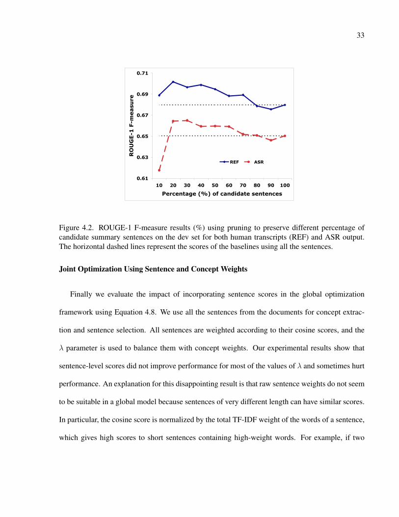
4.2 ROUGE-1 F-measure results (%) using pruning to preserve different percentage
of candidate summary sentences on the dev set for both human transcripts (REF)
and ASR output. The horizontal dashed lines represent the scores of the baselines
using all the sentences. . . . . . . . . . . . . . . . . . . . . . . . . . . . . . . . . 33
5.1 Illustration of up-sampling for binary classification. . . . . . . . . . . . . . . . . . 45
5.2 Illustration of down-sampling in binary classification. . . . . . . . . . . . . . . . . 48
5.3 Flowchart for re-sampling method. . . . . . . . . . . . . . . . . . . . . . . . . . . 49
5.4 Coverage of the original positive samples (left Y-axis) and the percentage of pos-
itive samples in the selected data (right Y-axis) using TFIDF and cosine scores as
selection criteria for different re-sampling rates. . . . . . . . . . . . . . . . . . . . 50
5.5 ROUGE-1 F-measure results (%) using up-sampling on human transcripts. . . . . . 56
5.6 ROUGE-1 F-measure results (%) using up-sampling on ASR outputs. . . . . . . . 57
5.7 ROUGE-1 F-measure results (%) using down-sampling on human transcripts. . . . 59
5.8 ROUGE-1 F-measure results (%) using down-sampling on ASR outputs. . . . . . . 59
5.9 ROUGE-1 F-measure results (%) using the re-sampling method. . . . . . . . . . . 61
5.10 ROUGE-1 F-measure results (%) using the regression model. . . . . . . . . . . . . 62
xv
6.1 ROUGE-1 F-measure results of co-training on the development using the models
trained from textual and prosodic features. . . . . . . . . . . . . . . . . . . . . . . 85
6.2 ROUGE-1 F-measure results of co-training results on the test using the models
trained from textual (upper) and prosodic features (lower). . . . . . . . . . . . . . 87
6.3 An example of confusion networks for a sentence segment. . . . . . . . . . . . . . 90
6.4 ROUGE-1 F-measure results using n-best lists (up to 50 hypotheses) on the devel-
opment set. . . . . . . . . . . . . . . . . . . . . . . . . . . . . . . . . . . . . . . 97
6.5 ROUGE-2 F-measure results using n-best lists (up to 50 hypotheses) on the devel-
opment set. . . . . . . . . . . . . . . . . . . . . . . . . . . . . . . . . . . . . . . 98
6.6 ROUGE-1 F-measure results using n-best lists (up to 50 hypotheses) on the de-
velopment set, with the summaries constructed using the corresponding human
transcripts of the selected hypotheses. . . . . . . . . . . . . . . . . . . . . . . . . 99
6.7 ROUGE-2 F-measure results using n-best list (up to 50 hypotheses) on the de-
velopment set, with the summaries constructed using the corresponding human
transcripts of the selected hypotheses. . . . . . . . . . . . . . . . . . . . . . . . . 100
6.8 Average node density and word coverage of the confusion networks on the devel-
opment set. . . . . . . . . . . . . . . . . . . . . . . . . . . . . . . . . . . . . . . 102
xvi

CHAPTER 1
INTRODUCTION
1.1 Motivation
With massive amounts of speech recordings and multimedia data available, an important prob-
lem is how to efficiently process these data to meet user’s information need. There has been
increasing interest recently in automatically processing the speech data, including summariza-
tion, and other understanding tasks in the research community (for example, programs such as
AMI/AMIDA, CHIL in Europe [1, 2], and CALO [3], and NIST’s Rich Transcription evaluation
on the meeting domain [4]).
Automatic summarization is a very useful technique to facilitate users to browse large amount
of data efficiently. Summarization can be divided into different categories along several different
dimensions [5]. Based on whether or not there is an input query, the generated summary can
be query-oriented or generic; based on the number of input documents, summarization can use a
single document or multiple documents; in terms of how sentences in the summary are formed,
summarization can be conducted using either extraction or abstraction — the former only selects
sentences from the original documents, whereas the latter involves natural language generation.
Overall, automatic summarization systems aim to generate a good summary, which is expected to
be concise, informative, and relevant to the original input.
A lot of techniques and approaches have been proposed for automatic text summarization the
1

2
past decades, and there are some benchmark tests such as TIDES, AQUAINT, MUC, DUC, and
TAC [6, 7, 8, 9, 10]. To summarize and process the speech data, a natural solution is to tran-
scribe the speech recordings to texts, and apply some well studied text summarization approaches.
However, usually when the traditional NLP methods are directly applied to speech transcripts, the
performance is not as good as for text processing. There are several issues that make the speech
transcripts different from the written texts.
• The speech transcripts often have a lot of disfluencies, while written texts are normally well
formed and organized. This is especially the case for spontaneous speech domains, such
as multiparty meetings, conversational telephone speech. Even for broadcast news, which
are read speech, they contain unavoidable disfluencies. In addition, there are often inserted
broadcast conversations which are more conversational.
• If we use the output of the automatic speech recognition (ASR) system for summarization,
the output is actually only word sequence, and there are no punctuation marks or sentence
segments associated with it. Therefore we first need to segment the word sequence into
pieces to use as summarization units. A simple way to do that is using acoustic segment
boundaries that correspond to long stretches of silence or a change of conversational turn.
There are other automatic methods to detect the sentence boundaries, which integrate more
linguistic information, such as language model score, part-of-speech tags, and etc. How-
ever, these automatically segmented sentences are still different from the human annotated
linguistic sentences. This often affects the down-streaming language understanding perfor-
mance.
• The speech transcripts contain word errors, especially for the conversational speech. For

3
example, for meeting recordings, the word error rate could be as high as around 40%. With
such lower accuracy, it is hard to read the transcripts and generate a summary even for human
annotators. If the cue words or cue phrases are not correctly recognized, it will have great
impact on the selection of important sentences.
All of these issues make speech summarization different from text summarization, and the tra-
ditional text summarization approaches generally do not perform well in speech summarization
task.
This thesis focuses on the task of extractive summarization using the meeting corpus. Given
the meeting document (a meeting recording together with its transcript), our aim is to select the
most important and representative parts, and concatenate them together to form a summary. Au-
tomatic summarization on the meeting domain is more challenging comparing to summarization
of other speech genres, such as broadcast news, lectures, and voice mail. Different from broadcast
news and lectures, which are read or pre-planed speech, meetings are more spontaneous, so the
meeting transcripts contain a lot of disfluencies, such as filled pauses, repetitions, revisions, and
etc. Although some meetings have pre-defined topics, in general the content of meetings is less co-
herent than other speech genres. For speech recognition, the ASR performance in meeting domain
is also worse than other speech domains. Such noisy data has great impact on the performance of
traditional summarization approaches.
1.2 Main Contributions
In this thesis, we exploited different methods for the task of extractive meeting summariza-
tion, including unsupervised, supervised, and semi-supervised approaches. We proposed improved

4
methods to address several issues in existing summarization approaches, as well as leverage speech
specific information for meeting summarization.
Two unsupervised frameworks were introduced and investigated in Chapter 4, maximum marginal
relevance (MMR) and the concept-based global optimization framework. Under the MMR frame-
work, other than the simple lexical matching, we evaluated different similarity measures to better
capture the semantic relationship between text segments. Better similarity measures can help de-
fine the importance of each sentence and its relationship with other sentences in the document.
The concept-based optimization framework selects a subset of summary sentences to maximize
the coverage of important concepts. We proposed to leverage the sentence level information in this
framework to improve the linguistic quality of extracted summaries.
In Chapter 5, supervised learning approaches were adopted, where the summarization task is
considered as a binary classification problem, summary or non-summary, and each sentence is
represented by a large set of features. We analyzed the feature effectiveness for both human and
ASR conditions. In addition, two important issues associated with this classification approach were
addressed. First, since the summary sentences are only a small portion of the entire document, there
is an imbalanced data problem during classifier training. The second problem is that the agreement
between different human annotators is very low. We proposed different sampling methods to solve
these problems by providing more balanced training data through changing the original labels
of the samples, or selecting a subset of balanced samples. We also proposed using a regression
model for this task, where the label for each sample is not binary any more, but a numerical value
representing its importance.
Chapter 6 addressed several issues specific to speech summarization. Since the speech record-

5
ings are available, in Section 6.1, we investigated whether we can extract more features from
speech data to help improve the summarization performance. These features include pitch, energy,
sentence duration, speaking rate, and their different normalized variants. We showed that using
only the prosodic information we can generate a better summarizer than using the textual infor-
mation. The textual and acoustic features can be naturally split into two conditional independent
sets, and each of them is sufficient to generate a good summarizer. In Section 6.2, we adopted
the co-training algorithm so that we can obtain good summarization performance by only using a
small amount of labeled data and extra unlabeled data for training.
Because of the high word error rates in meeting transcripts, we found that using the ASR
output often degrades the summarization performance comparing to using the human annotated
transcripts. In Section 6.3, we demonstrated the feasibility of using rich speech recognition results
to improve the speech summarization performance. Two kinds of structures were considered, n-
best hypotheses and confusion networks. Under an unsupervised MMR framework, we proposed
the term weighting and vector representation methods to reframe the text segments considering
more word candidates and sentence hypotheses.

CHAPTER 2
RELATED WORK
In this chapter, we provide a literature review of previous research related to automatic speech
summarization. We limit our survey to speech summarization, since the focus of this thesis is
extractive meeting summarization.
Automatic speech summarization has received a lot of attentions in recent years, and different
speech domains have been explored. Broadcast news speech is the first domain to be exploited for
speech summarization [11]. This domain is similar to the news article domain widely used for text
summarization, but is different as it consists of read and spontaneous speech, and there are speech
recognition errors (though generally lower than other speech genres), thus presents a good starting
point to evaluate the portability of the classical features and approaches used in text summarization.
Research was then expanded to lecture speech summarization [12]. Lectures are much longer
than broadcast news, and contain more spontaneous speech. However, the slides associated with
the lectures provide additional information for selecting the summary sentences. Comparing to
the previous two speech genres, meeting speech is the most spontaneous one, and often involves
multiple speakers [13]. Recently there have been many efforts on various meeting understanding
tasks, such as automatic summarization, meeting browsing, detection of decision parts and action
items, topic segmentation, keyword extraction, and dialog act tagging [13, 14, 15, 16, 17, 18].
Other speech genres used for summarization include television shows, conversational telephone
speech, and voice mail [19, 20, 21].
6

7
In the following sections, we first introduce the state-of-the-art approaches used for automatic
extractive speech summarization. Then we briefly describe the recent activities of generating ab-
stractive summaries. Last, we discuss research on evaluation metrics for summarization perfor-
mance.
2.1 Extractive Speech Summarization
2.1.1 Unsupervised Approaches
Unsupervised approaches are relatively simple, and robust to different corpora. The summary
sentences are usually selected according to their own importance, and their relationship to other
sentences in the document. In [22], the authors proposed to select important utterances or n-grams
using each word’s inverse document frequency and acoustic confidence score, and found that this
can help the summarizer select more accurate utterances. In [23], the summary sentences were
extracted according to a sentence’s significance score measured using TFIDF, trigram probability
of the sentence, and confidence score from the ASR system.
In the above two approaches, the summary sentences were selected based only on their individ-
ual significance. Other than the sentence importance, the relationship between sentences should
also be considered during the sentence selection, since the generated summary should be concise
and representative, and no redundant information should be included. MMR was introduced in
[24] for text summarization, and has been applied to speech summarization. This algorithm can
select the most relevant sentences, and at the same time avoid the redundancy by removing the
sentences that are too similar to the already selected ones. The summary sentences are selected

8
iteratively, and the weight for each sentence is calculated using the following equation:
MMR(Si) = λ× Sim1(Si, D)− (1− λ)× Sim2(Si, Summ) (2.1)
where D is the document vector, Summ represents the sentences that have been extracted into
the summary, and λ is used to adjust the combined score to emphasize the relevance or to avoid
redundancy. In [25], the authors compared the MMR method with two other approaches: one
selecting the sentences similar to the first sentence, and the other selecting sentences that are most
similar to the entire document. They showed that the MMR method outperformed the other two
on spontaneous speech summarization.
Latent semantic analysis (LSA) approach has been used in extracting the summary sentences by
exploring the semantic similarity between sentences considering a set of latent topics [13]. In this
method, a set of latent topics T1, T2, . . . , TK is first defined, and then each word in the document is
modeled to be generated from these latent topics.
P (wi|D) =K∑k=1
P (wi|Tk)P (Tk|D) (2.2)
In [26], the authors proposed two methods under LSA, topic significance and term entropy, where
the important terms were detected and given higher weights during calculation. The term impor-
tance was calculated according to the term’s distribution in a large corpus, or term entropy over the
latent topics. They found that their proposed methods obtained better summarization performance
comparing to the original LSA method.
In [27], the authors introduced a concept-based global optimization framework, where concepts
were used as the minimum units, and the important sentences were extracted to cover as many

9
concepts as possible. A global optimization function was defined as following:
maximize∑i
wici (2.3)
subject to∑j
ljsj < L (2.4)
where wi is the weight of concept i, ci is a binary variable indicating the presence of that concept
in the summary, lj is the length of sentence j, L is the desired summary length, and sj represents
whether a sentence is selected for inclusion in the summary. Integer linear programming method
was used to select sentences that maximize the objective function under the length constraint L.
The authors showed that this global optimization method outperformed MMR.
Graph-based methods, such as LexRank [28], represent a document using a graph, where sen-
tences are modeled as nodes. Then the summary sentences are ranked according to their similarities
with other nodes. [29] proposed ClusterRank, a modified graph-based method, to cope with high
noise and redundancy in spontaneous speech transcripts. In ClusterRank, the neighbor sentences
were first clustered according to their cosine similarity scores, and the graph was constructed on
these clusters. The similarity between clusters was calculated by only considering the important
words contained in the cluster. The authors showed better performance of using ClusterRank than
LexRank. In [30], the authors suggested formulating the summarization task as optimizing sub-
modular functions defined on the document’s semantic graph. The construction of the graph was
similar to LexRank, where sentences were modeled as nodes, and similarities between nodes as
edge weights. The optimization was theoretically guaranteed to be near-optimal under the frame-
work of submodularity. The authors achieved significantly better results than using MMR and the
concept-based global optimization framework.

10
2.1.2 Supervised Approaches
Another line of work for extractive speech summarization is based on supervised methods,
where all the utterances in a document are divided into two classes, in summary or not, then the
summarization task can be considered as a binary classification problem. Although a large amount
of labeled data is necessary for training the classifier, supervised approaches usually achieve bet-
ter performance comparing to the unsupervised ones. Various models have been investigated for
this classification task, such as Bayesian network [31], maximum entropy [32], support vector ma-
chines (SVM) [20], hidden Markov model (HMM) [33], and conditional random fields (CRF) [34].
In [13], Murray et al. compared MMR, LSA, and the feature-based classification approach, and
showed that human judges favor the feature-based approaches.
In [31], the authors constructed a summarizer using the structural features. Different from text
summarization, other than sentence position and sentence length, the authors included the speaker-
related features, which represent the overall contribution of each speaker. The authors reported
that the system was robust to the speech recognition errors by comparing the results obtained from
using manual transcripts and ASR outputs. In [35], the authors provided an empirical study of the
usefulness of different types of features in the domain of broadcast news summarization, including
lexical, acoustic/prosodic, structural, and discourse features. The lexical and discourse features
are also commonly used in text summarization, such as the count of name entities, the number of
words in the sentence, and the features representing the word distributions. The structural features
were similar as introduced in [31], which include the speaker information. The acoustic/prosodic
features are unique for speech summarization, which are extracted from the speech recordings. The
authors pointed out that a change in pitch, amplitude or speaking rate may signal differences in the

11
relative importance of the speech segments. Experimental results showed that a combination of all
the features performs the best. However, acoustic/prosodic and structural features were enough to
build a “good” summarizer when speech transcripts are not available.
In [36], the authors compared the contribution of different types of features in conversational
speech summarization using the Switchboard data. Other than the features mentioned before, they
included MMR scores of each sentence, and a set of spoken-language features. These spoken-
language features contained the number of repetitions and filled pauses, which can better capture
the characteristics of more spontaneous speech. Their experiments showed that speech disfluen-
cies helped identify important utterances, while the structural features are less effective than in
broadcast news.
In [37], the authors introduced the rhetorical information for lecture summarization. Since lec-
tures and presentations are planned speech and follow a relatively rigid rhetorical structure, the
authors proposed to use a hidden Markov model to learn this rhetorical structure trained on the
slides associated with the speech, and features were then extracted for each structure. They proved
that using rhetorical structure improved the summarization performance. They also showed that
lexical features were more important than acoustic features, and different from broadcast news and
conversational speech summarization, discourse features were not useful for lecture summariza-
tion.
On the task of meeting summarization, Murray et al. [38] analyzed the speaker activity, turn-
taking, and discourse cues, and reported that using these features was advantageous and efficient
than only using the textual features.
The contribution of different types of features varies according to different speech genres. In

12
[12], the authors compared the lexical, structural, and acoustic features on speech summarization
of Mandarin broadcast news and lecture speech. They found that structural features were superior
to acoustic and lexical features when summarizing broadcast news, but acoustic and structural
features made more important contribution to broadcast news summarization comparing to lecture
summarization.
2.1.3 Other Approaches
Other than unsupervised and supervised approaches, previous research investigated the ways
that can combine the unsupervised and supervised methods. The results from unsupervised meth-
ods can be considered as one of the features for supervised learning. For example, in [39], the
MMR results were used as features for supervised training. In [40], the authors formulated extrac-
tive summarization as a risk minimization problem and proposed a unified probabilistic framework
that naturally combined the supervised and unsupervised approaches. The summary sentences
were selected using the following function:
S = argminSi∈D∑Sj∈D
L(Si, Sj)P (D|Sj)P (Sj)∑
Sm∈D P (D|Sm)P (Sm)(2.5)
where D is the document to be summarized, and Si is one of the sentences contained in D.
P (D|Sj) can be modeled as a sentence generative model, where the probability is calculated us-
ing the product of each word’s generative model P (w|Sj). The sentence prior probability P (Sj)
was in proportion to the posterior probability of the sentence being included in the summary class
obtained from a supervised learning classifier. The concept of MMR was incorporated into the
computation of loss function L(Si, Sj). Such a framework can be regared as a generalization of
several existing summarization methods. The authors showed significant improvements over sev-
eral popular summarization methods, such as vector space model, LexRank, and CRF.

13
2.2 From Extractive to Abstractive Summarization
The extracted summary sentences often contain a lot of disfluencies, and may have word er-
rors if the input for summarization is automatically recognized transcripts. Simply concatenating
extracted sentences may not comprise a good summary. Other than extractive summarization, re-
searchers also worked on generating abstractive summaries, or compressing the extracted sentences
and merging them into a more concise summary.
Instead of post-processing the extractive summary sentences, some previous research removed
the disfluencies in the documents before performing summarization [41]. The types of disfluencies
were difined as filled pauses, restarts or repairs, and false starts. A part-of-speech tagger was
trained to detect the filled pauses, and the words tagged with CO (coordinating), DM (discourse
marker), and ET (editing term), were removed from the texts. The false starts were detected using
a decision tree, and a rule-based script was used to detect the repetition. After pre-processing the
speech transcripts, MMR was used to select the important summary sentences.
In [42], for each sentence, a set of words maximizing a summarization score was extracted
from automatically transcribed speech. This extraction was performed using a dynamic program-
ming technique. The summarization score consisted of a word significance measure, a confidence
measure, linguistic likelihood, and a word concatenation probability which was determined by a
dependency structure in the original speech. These word sequences were then concatenated to
form a summary. The disfluencies and possible errorful words will be automatically removed from
the summary because the word sequence was selected considering acoustic confidence scores and
linguistic likelihood.
In [43], the abstractive summaries were generated by applying sentence compression on se-

14
lected extractive summary sentences. The authors proposed several compression methods. First
the filler phrases were detected and removed, which could be discourse markers (e.g., I mean, you
know), editing terms, as well as some terms that are commonly used by human but without critical
meaning, such as, “for example”, “of course”, and “sort of”. Then an integer programming based
framework was introduced, where the word sequence was selected maximizing the sum of the
significance scores of the consisting words and n-gram probabilities from a language model. The
experimental results showed that further compression of the extractive summaries can improve the
summarization performance.
In [44], the authors developed an abstractive conversation summarization system consisting of
interpretation and transformation components. In the interpretation component, each sentence
is mapped to a simple conversation ontology, where conversation participants and entities are
linked by object properties, such as decisions, actions, and subjective opinions. In the trans-
formation step, a summary is created by maximizing a function relating sentence weights and
entity weights. The authors pointed out that these selected summary sentences corresponded to
< participant, relation, entity > triplets in the ontology, for which they can subsequently gener-
ate novel text by creating linguistic annotations of the conversation ontology. This result can also
be used to generate structured extracts by grouping sentences according to specific phenomena
such as action items and decisions.
2.3 Summarization Evaluation
How to properly evaluate summarization results automatically is still an open topic. Sum-
marization evaluation techniques can generally be classified as intrinsic or extrinsic evaluation.

15
Intrinsic evaluation compares the system generated summaries with gold-standard human sum-
maries. Extrinsic metrics, on the other hand, evaluate the usefulness of the summary in performing
a real-world task. Most of the summarization work evaluates their performance using intrinsic
measures, because such evaluations are easily replicable and more useful for development pur-
poses.
ROUGE [45] has been widely used in previous research and benchmark summarization tests
(e.g., DUC). ROUGE compares the system generated summary with reference summaries (there
can be more than one reference summary), and measures different matches, such as N-gram,
longest common sequence, and skip bigrams. For example, ROUGE-N is an n-gram recall be-
tween a candidate summary and a set of reference summaries computed as follows:
ROUGE −N =
∑S∈ReferenceSummaries
∑gramn∈S Countmatch(gramn)∑
S∈ReferenceSummaries∑
gramn∈S Count(gramn)(2.6)
However, some research showed that in general the correlation of ROUGE scores and human
evaluation is low for some speech domains [46, 47].
In [48], the authors proposed a pyramid method for summarization evaluation based on Sum-
marization Content Units (SCU). The annotation starts with identifying similar sentences, and then
SCUs are extracted by inspecting and identifying more tightly related subparts. Each SCU has a
weight corresponding to the number of summaries it appears in. After the annotation procedure is
completed, a pyramid is built based on the weight of each SCU. The score for the automatically
generated summary is assigned as a ratio of the sum of the weights of its SCUs to the sum of the
weights of an optimal summary with the same number of SCUs. This pyramid method not only
assigns a score to a summary, but also allows the investigator to find what important information
is missing, and thus can be directly used to target improvements of the summarizer. However,

16
creating an initial pyramid is very laborious. In [34], the authors adopted this Pyramid evaluation
metric but with the constraints that two summary units are considered equivalent if and only if they
are extracted from the same location in the original document.
In [38], the authors proposed to evaluate the summarization performance using weighted pre-
cision and recall at the dialog act level, which utilized the particular summary annotation of the
corpus they used in their study. The evaluation was conducted according to how often each anno-
tator linked a given extracted dialog act to a summary sentence. The weighted precision, recall and
f-score were calculated as the final score for the summary to be evaluated.

CHAPTER 3
CORPUS AND EVALUATION MEASUREMENT
The data we use in this thesis is the ICSI meeting corpus [49]. It contains 75 recordings from
natural meetings (most are research discussions in speech, AI, and networking areas) [49]. Each
meeting is about an hour long and has multiple speakers. These meetings have been transcribed,
annotated with dialog acts (DA) [50], topic segmentation, and extractive summaries [46]. For ex-
tractive summary annotation, the annotators were asked to select and link DAs from the transcripts
that are related to each of the sentences in the provided abstractive summaries (see [46] for more
information on annotation). Figure 3.1 shows a sample from one of the human transcripts, where
each line corresponds to a DA, and the ID at the beginning of each line (marked by S*) is the
speaker ID. In this excerpt, three sentences (18, 19, and 25) were marked as the summary sen-
tences by the annotator. From this example, we can see the meeting transcripts are significantly
different from the input for text summarization (e.g., news article) in that it is very spontaneous,
contains disfluencies and incomplete sentences, has low information density, and involves multiple
speakers.
The automatic speech recognition (ASR) output for this corpus is obtained from a state-of-the-
art SRI conversational telephone speech system [51, 52]. The word error rate is about 38.2% on
the entire corpus. We align the human transcripts and ASR output, then map the human annotated
DA boundaries and topic boundaries to the ASR words, such that we have human annotation for
the ASR output. For the extractive summarization task, we use human annotated DA boundaries
17

18
[1] S1 yeah if you breathe under breathe and then you see af go off then you know -pau- it's p- picking up your mouth noise [laugh][2] S2 oh that's good[3] S2 cuz we have a lot of breath noises[4] S3 yep[5] S3 test [laugh][6] S2 in fact if you listen to just the channels of people not talking it's like [laugh][7] S2 it's very disgust-[8] S3 what[9] S3 did you see hannibal recently or something[10] S2 sorry[11] S2 exactly[12] S2 it's very disconcerting[13] S2 ok[14] S2 so um[15] S2 i was gonna try to get out of here like in half an hour[16] S2 um[17] S2 cuz i really appreciate people coming*[18] S2 and the main thing that i was gonna ask people to help with today is -pau- to give input on what kinds of database format we should -pau- use in starting to link up things like word transcripts and annotations of word transcripts*[19] S2 so anything that transcribers or discourse coders or whatever put in the signal with time-marks for like words and phone boundaries and all the stuff we get out of the forced alignments and the recognizer[20] S2 so we have this um[21] S2 i think a starting point is clearly the the channelized -pau- output of dave gelbart's program[22] S2 which don brought a copy of[23] S3 yeah[24] S3 yeah i'm i'm familiar with that*[25] S3 i mean we i sort of already have developed an xml format for this sort of stuff[26] S2 um[27] S2 which[28] S1 can i see it[29] S3 and so the only question is it the sort of thing that you want to use or not[30] S3 have you looked at that[31] S3 i mean i had a web page up[32] S2 right
Figure 3.1. An excerpt of meeting transcripts with summary information.

19
as sentence information and perform sentence-based extraction. The ASR output for the same
example as in Figure 3.1 is shown in Figure 3.2. We can see a lot of recognition errors in this
example.
Figure 3.2. ASR output for the excerpt shown in Figure 3.1.
The same 6 meetings as in previous work (e.g., [13, 27, 30, 53]) are used as the test set in this
study. Furthermore, 6 other meetings were randomly selected from the remaining 69 meetings
in the corpus to form a development set, then the rest is used to compose the training set for
the supervised learning approach. Each of the meetings in the training and development set has
only one human-annotated summary, whereas for the test meetings, we use 3 reference summaries

20
from different annotators for evaluation. For summary annotation, human agreement is quite low
[54]. The average Kappa coefficients among these 3 annotators on the test set ranges from 0.211
to 0.345. The lengths of the reference summaries are not fixed and vary across annotators and
meetings. The average word compression ratio for the test set is 14.3%, and the mean deviation is
2.9%. These statistics are similar for the training set.
In our study we use ROUGE as the evaluation metrics because it has been used in previous
studies of speech summarization, and thus we can compare our work with previous results [13,
20, 27, 34, 35, 37, 40]. The options we used in this study are the same as those used in DUC:
stemming summaries using Porter stemmer before computing various statistics (-m); averaging
over the sentence unit ROUGE scores (-t 0); assigning equal importance to precision and recall (-p
0.5); computing statistics in the confidence level of 95% (-c 95) based on sampling points of 1000
in bootstrap resampling (-r 1000).

CHAPTER 4
UNSUPERVISED APPROACHES FOR EXTRACTIVE MEETING SUMMARIZATION
In this chapter, we study two unsupervised approaches for extractive meeting summariza-
tion, maximum marginal relevance (MMR) and a concept-based global optimization framework.
Among all the approaches for summarization, MMR is one of the simplest techniques, and has
been effectively used for text and speech summarization [24]. The extractive summarization prob-
lem can also be modeled using a global optimization framework based on the assumption that
sentences contain independent concepts of information, and that the quality of a summary can be
measured by the total value of unique concepts it contains [27]. In this chapter, we propose im-
proved solutions for these two unsupervised methods to obtain better summarization performance.
4.1 Using Corpus and Knowledge-based Similarity Measure in MMR
4.1.1 Maximum Marginal Relevance (MMR)
MMR is a greedy algorithm, where the summary sentences with the highest scores are selected
iteratively as we introduced in Section 2.1.1. The score is calculated using two similarity functions
(Sim1 and Sim2), as shown in Equation 2.1, representing the similarity of a sentence to the entire
document and to the selected summary, respectively. We adopt two approximated methods to speed
up the process of calculating the MMR scores [55]. For each sentence, we calculate its similarity to
all the other sentences that have a higher similarity score to the document (according to the results
21

22
of Sim1), and use it as an approximation for Sim2. Therefore, the summary selection process
only needs to find the top sentences that have high combined scores, which is a offline processing.
Another approximation we use is not to consider all the sentences in the document, but rather only
a small percent of sentences (based on a predefined percentage) that have a high similarity score to
the entire document. Our hypothesis is that the sentences that are closely related to the document
are worth being selected.
4.1.2 Similarity Measures
An important part in MMR is how we can appropriately represent the similarity of two text
segments. In this section, we evaluate three different similarity measures.
Cosine Similarity
One commonly used similarity measure is cosine similarity, which we use as our baseline in
this study. In this approach, each document (or a sentence) is represented using a vector space
model. The cosine similarity between two vectors (D1, D2) is:
sim(D1, D2) =
∑i t1it2i√∑
i t21i ×
√∑i t
22i
(4.1)
where ti is the term weight for a word wi, for which we use the TF-IDF (term frequency, inverse
document frequency) value, as widely used in information retrieval. The IDF weighting is used to
represent the specificity of a word: a higher weight means a word is specific to a document, and a
lower weight means a word is common across many documents. IDF values are generally obtained
from a large corpus as follows:
IDF (wi) = log(N/Ni) (4.2)

23
where Ni is the number of documents containing wi in a collection of N documents. In [56],
Murray and Renals compared different term weighting approaches to rank the importance of the
sentences (simply based on the sum of all the term weights in a sentence) for meeting summariza-
tion, and showed that TF-IDF weighting is competitive.
Centroid Score
Another distance measure we evaluate is the centroid score [55], which only considers the
salient words for the similarity between a sentence and the entire document. The same vector
representation is used as in cosine similarity. In this approach, each word in a sentence Si is
checked to see if it occurs in the text segment T and if the term weight (TF-IDF value) of this word
is greater than a predefined threshold. If these requirements are met, the term weight of this word
is added to the centroid score for the sentence.
Scorecentroid(i) =∑wj∈Si
bool(wj ∈ T ) ∗ bool(tw(wj) > v) ∗ tw(wj) (4.3)
where tw(wj) represents the term weight for the word wj , and the functions bool(wj ∈ T ) and
bool(tw(wj) > v) check the two conditions mentioned above. In the MMR system, we use the
centroid score as the first similarity function (Sim1 in Equation 2.1). The second similarity mea-
sure Sim2 is still the cosine distance.
Corpus-based Semantic Similarity
The cosine and centroid scores between a sentence and a document are all based on simple
lexical matching, that is, only the words that occur in both contribute to the similarity. Such literal

24
comparison can not always capture the semantic similarity of text. Therefore we use the following
function to compute the similarity score between two text segments [57].
sim(T1, T2) =1
2(
∑w∈{T1}
(maxSim(w, T2) ∗ idf(w))∑w∈{T1}
idf(w)+
∑w∈{T2}
(maxSim(w, T1) ∗ idf(w))∑w∈{T2}
idf(w)) (4.4)
maxSim(w, Ti) = maxwi∈{Ti}
{sim(w,wi)} (4.5)
For each word w in segment T1, we find a word in segment T2 that has the highest semantic
similarity to w (maxSim(w, T2)). Similarly, for the words in T2, we identify the corresponding
words in segment T1. The similarity score of the two text segments is then calculated by combining
the similarity of the words in each segment, weighted by their word specificity (i.e., IDF values).
To calculate the semantic similarity between two words w1 and w2, we use a corpus-based
approach and measure the pointwise mutual information (PMI) [57, 58]:
PMI(w1, w2) = log2c(w1 near w2)
c(w1) ∗ c(w2)(4.6)
This indicates the statistical dependency between w1 and w2, and can be used as a measure of the
semantic similarity of two words. c(w1 near w2) represents the number of times that word w1
appears near word w2. For this co-occurrence count, a window of length l is used, that is, we only
count when w1 and w2 co-occur within this window. For a word, we define PMI(w,w) = 1,
therefore, maxSim(w, T ) is 1 if w appears in T .
The part-of-speech (POS) information of each word can also be taken into consideration when
calculating the similarity of two text segments [57]. Then Equation 4.5 can be modified as:
maxSim(w, Ti) = maxwi∈{Ti},pos(wi)=pos(w)
{sim(w,wi)} (4.7)

25
This means when finding the maxSim between a word w and a text segment Ti, we will only
consider the words in Ti with the same POS as word w. The reason behind this is that it is more
meaningful to calculate the similarity of two words with the same POS.
Note that two different words in the two segments also contribute to the similarity score using
this corpus-based approach. We call this approach corpus-based similarity following [57], even
though in the cosine and centroid scores, the IDF values are also generated based on a corpus. For
the MMR score, we use the corpus-based similarity for the two similarity functions (Sim1, Sim2)
in Equation 2.1, since it is more comparable than using a corpus-based similarity for Sim1 and a
cosine similarity for Sim2.
4.1.3 Experimental Results and Discussion
Experimental Setup
The IDF values are obtained from the 69 training meetings. We split each of the 69 training
meetings into multiple topics, and then use these new “documents” to calculate the IDF values.
This generates more robust estimation for IDF, compared with simply using the original 69 meet-
ings as the documents. We calculated different IDF values for the human transcripts and ASR
outputs respectively, which will be used according to different transcripts. The PMI information is
also generated for both the human transcripts and ASR outputs respectively.
We tagged all the meetings using the TnT POS tagger [59]. The POS model is retrained using
the Penn Treebank-3 Switchboard data, which is expected to be more similar to the meeting style
than domains such as Wall Street Journal.
Since the length of reference summaries varies across different annotators and meeting docu-

26
ments, in our experiments we generated summaries with the word compression ratio ranging from
14% to 18%.
Experimental Results
We evaluate the different approaches for similarity measure under the MMR framework for
meeting summarization. Table 4.1 shows the summarization results (ROUGE unigram match R-1)
using human transcripts for different compression ratios on the test set. The columns Sim1 and
Sim2 are the similarity measures we used for the two similarity functions in Equation 2.1, which
represent the similarity of a sentence Si to the whole document, and the similarity of the sentence
Si to the currently selected summary, respectively.
Table 4.1. ROUGE-1 F-measure results (%) using different similarity approaches on test set usinghuman transcripts.
Sim1 Sim2 14% 15% 16% 17% 18%cosine cosine 65.69 66.23 66.69 66.70 66.38
centroid cosine 68.28 68.48 69.02 68.99 68.76corpus corpus 68.65 69.16 68.92 68.54 68.30
corpus pos corpus pos 69.66 69.89 70.08 69.71 68.99
Among the different similarity measures, both the centroid and the corpus-based similarity
measures outperform the cosine similarity. Adding POS constraint for word similarity is also
helpful, achieving the best performance among all the approaches. When POS information is
considered in the corpus-based similarity measure, there is a further improvement.
Table 4.2 shows the results using ASR output on the test set. We notice that there is a per-
formance degradation compared to using reference transcripts, but the new proposed similarity
measure still outperforms the baseline. In the corpus-based method, considering POS information

27
does not improve the system performance, different from what have observed on the human tran-
script condition. This is probably because the POS tagging accuracy for the ASR transcripts is
relatively low∗, which impacts the word similarity in Equation 4.5.
Table 4.2. ROUGE-1 F-measure results (%) using different similarity approaches on test set usingASR output.
Sim1 Sim2 14% 15% 16% 17% 18%cosine cosine 62.37 63.36 63.91 64.22 64.60
centroid cosine 63.41 64.24 64.78 64.96 65.05corpus corpus 63.86 64.52 64.85 65.01 65.12
corpus pos corpus pos 61.90 62.73 63.18 63.59 63.75
4.2 Leveraging Sentence Weights in Global Optimization Framework †
The MMR method we used in the previous section is local optimal because the decision is made
based on the sentences’ scores in the current iteration. In [60], the author studied modeling the
multi-document summarization problem using a global inference algorithm with some definition
of relevance and redundancy. The Integer Linear Programming (ILP) solver was used to efficiently
search a large space of possible summaries for an optimal solution. In [27], the authors adopted this
global optimization framework assuming that concepts are the minimum units for summarization,
and summary sentences are selected to cover as many concepts as possible. They showed better
performance than MMR. However, this method tends to select short sentences with fewer concepts
in order to increase the number of concepts covered, instead of selecting sentences rich in concepts
even if they overlap. According to manual examination, this seems to result in the degradation
∗The meeting corpus is not annotated with POS information, so we cannot evaluate the POS tagging performance.†Joint work with Benoit Favre and Dilek Hakkani-Tur

28
of the linguistic quality of the summary. In this section, we propose to incorporate and leverage
sentence importance weights in the concept-based optimization method, and investigate different
ways to use sentence weights.
4.2.1 Concept-based Summarization
First, we use a similar framework as in [27] to build the baseline system for this section. The
optimization function is the same as Equation 2.3 and 2.4 introduced in Section 2.1.1. In our
research, we use the following procedure for concept extraction, which is slightly different from
the previous work in [27], where they used the rule-based algorithm for concept selection.
• Extract all content word n-grams for n = 1, 2, 3.
• Remove the n-grams appearing only once.
• Remove the n-grams if one of its word’s idf value is lower than a predefined threshold.
• Remove the n-grams enclosed by other higher-order n-grams, if they have the same fre-
quency. For example, we remove “manager” if its frequency is the same as “dialogue man-
ager”.
• Weight each n-gram ki as
wi = frequency(ki) ∗ n ∗maxj idf(wordj)
where n is the n-gram length, and wordj goes through all the words in the n-gram.
The IDF values are also calculated using the new “documents“ split according to the topic
segmentation as described in Section 4.1.2. Unlike [27], we use the IDF values to remove less in-
formative words instead of using a manually generated stopword list, and also use IDF information

29
to compute the final weights of the extracted concepts. Furthermore, we do not use WordNet or
part-of-speech tag constraints during the extraction. Therefore, using this new algorithm, the con-
cepts are created automatically, without requiring much human knowledge. We use this method as
the baseline for our research in the section.
4.2.2 Using Sentence Importance Weight
We propose to incorporate sentence importance weights in the above summarization frame-
work. Since the global optimization model is unsupervised, in this study we choose to use sentence
weights that can also be obtained in an unsupervised fashion. We use the cosine similarity scores
between each sentence and the entire document, which is also adopted as the baseline in the MMR
method calculated using Equation 4.1. We investigate different ways to leverage these sentence
scores in the concept-based optimization framework.
Filtering Sentences for Concept Generation
First we use sentence weights to select important sentences, and then extract concepts from the
selected sentences only. The concepts are obtained in the same way as described in Section 4.2.1.
The only difference is that they are generated based on this subset of sentences, instead of the entire
document. Once the concepts are extracted, the optimization framework is the same as before.
Pruning Sentences from the Selection
Sentence weights can also be used to filter unlikely summary sentences and pre-select a subset
of candidate sentences for summarization, rather than considering all the sentences in the doc-
30
ument. We use the same method to generate the summary as in Section 4.2.1, but only using
preserved candidate sentences.
Joint Optimization Using Sentence and Concept Weights
Lastly, we extend the optimization function (Equation 2.3) to consider sentence importance
weights, i.e.,
maximize (1− λ) ∗∑i
wici + λ ∗∑j
ujsj (4.8)
where uj is the weight for sentence j, λ is used to balance the weights for concepts and sentences,
and all the other notations are the same as in Equation 2.3. The summary length constraint is the
same as Equation 2.4. After adding the sentence weights in the optimization function, this model
will select a subset of relevant sentences which can cover the important concepts, as well as the
important sentences.
4.2.3 Experimental Results
We first use the development set to evaluate the effectiveness of our proposed approaches and
the impact of various parameters in those methods, and then provide the final results on the test
set.
Baseline Results
Several baseline results are provided in Table 4.3 using different word compression ratios for
both human transcripts and ASR output on the development set. The first one (long sentence) is
to construct the summary by selecting the longest sentences, which has been shown to provide

31
competitive results for meeting summarization task [39]. The second one (MMR ) is using cosine
similarity as the similarity measure on the MMR framework. The last result (concept-based ) is
from the concept-based algorithm introduced in Section 4.2.1. These scores are comparable with
those presented in [27]. For both human transcripts and ASR output, the longest-sentence baseline
is worse than the greedy MMR approach, which, in turn, is worse than the concept-based algorithm.
The performance on human transcripts is consistently better than on ASR output because of the
high WER. In the following experiments, we will use the concept-based summarization results as
the baseline, and a 16% word compression ratio.
Table 4.3. ROUGE-1 F-measure results (%) of three baselines on the dev set for both humantranscripts (REF) and ASR output.
compression 14% 15% 16% 17% 18%
REFlong sentence 54.50 56.16 57.47 58.58 59.23
MMR 66.81 67.06 66.90 66.64 66.09concept-based 67.20 67.98 68.30 67.82 67.51
ASRlong sentence 63.11 64.01 64.72 64.65 64.89
MMR 63.60 64.32 64.80 65.03 65.14concept-based 63.99 65.04 65.45 65.44 65.30
Filtering Sentences for Concept Generation
In Figure 4.1, we show the results on the development set using different percentages of impor-
tant sentences for concept extraction. When the percentage of the sentences is 100%, the result is
the same as the baseline using all the sentences. We observe that using a subset of important sen-
tences outperforms using all the sentences for both human transcripts and ASR output. For human
transcripts, using 30% sentences yields the best ROUGE score 0.6996, while for ASR output, the
best result, 0.6604, is obtained using 70% sentences.

32
0.60
0.62
0.64
0.66
0.68
0.70
10 20 30 40 50 60 70 80 90 100
Percentage (%) of important sentences
RO
UG
E-1
F-m
easu
re
REF ASR
Figure 4.1. ROUGE-1 F-measure results (%) using different percentage of important sentencesduring concept extraction on the dev set for both human transcripts (REF) and ASR output. Thehorizontal dashed lines represent the scores of the baselines using all the sentences.
Pruning Sentences from the Selection
This experiment evaluates the impact of using sentence weights to prune sentences and pre-
select summary candidates. Figure 4.2 shows the results of preserving different percentages of
candidate sentences in the concept-based optimization model. For this experiment, we use the
concepts extracted from the original document. For both human transcripts and ASR output, using
a subset of candidate sentences can significantly improve the performance, where the best results
are obtained using 20% candidate sentences for human transcripts and 30% for ASR output. We
also evaluate a length-based sentence selection and find that it is inferior to sentence score based
pruning.
33
0.61
0.63
0.65
0.67
0.69
0.71
10 20 30 40 50 60 70 80 90 100
Percentage (%) of candidate sentences
RO
UG
E-1
F-m
easu
re
REF ASR
Figure 4.2. ROUGE-1 F-measure results (%) using pruning to preserve different percentage ofcandidate summary sentences on the dev set for both human transcripts (REF) and ASR output.The horizontal dashed lines represent the scores of the baselines using all the sentences.
Joint Optimization Using Sentence and Concept Weights
Finally we evaluate the impact of incorporating sentence scores in the global optimization
framework using Equation 4.8. We use all the sentences from the documents for concept extrac-
tion and sentence selection. All sentences are weighted according to their cosine scores, and the
λ parameter is used to balance them with concept weights. Our experimental results show that
sentence-level scores did not improve performance for most of the values of λ and sometimes hurt
performance. An explanation for this disappointing result is that raw sentence weights do not seem
to be suitable in a global model because sentences of very different length can have similar scores.
In particular, the cosine score is normalized by the total TF-IDF weight of the words of a sentence,
which gives high scores to short sentences containing high-weight words. For example, if two
34
one-word sentences with a score of 0.9 are in the summary, they contribute 1.8 to the objective
function while one two-word sentence with a better score of 1.0 only contributes 1.0 to the sum-
mary. To eliminate this problem, raw cosine scores need to be rescaled to ensure a fair comparison
of sentences of different length. Therefore, in addition to using raw cosine similarity scores as the
weights for sentences, we consider two variations: multiplying the cosine scores by the number of
concepts and the number of words in that sentence, respectively.
Table 4.4. ROUGE-1 F-measure results (%) on the dev set for both human transcripts (REF) andASR output.
baseline raw cosine #concept norm #words normREF 68.30 68.42 68.42 68.50ASR 65.45 61.12 65.08 66.29
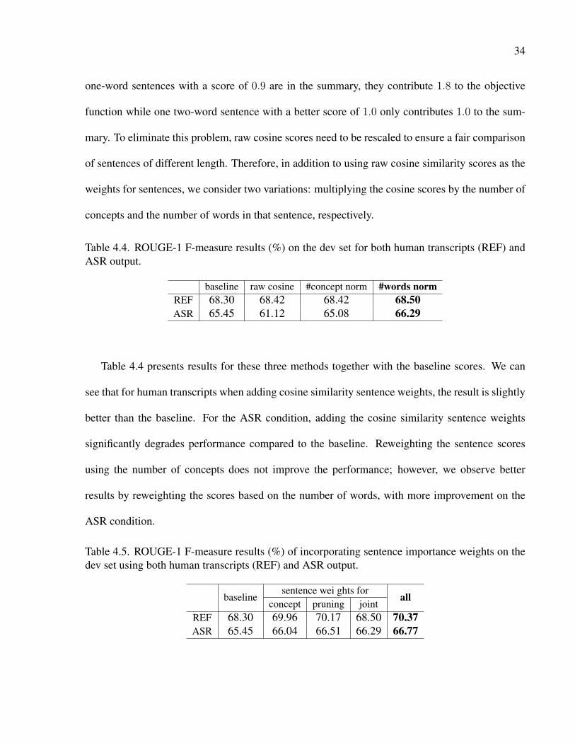
Table 4.4 presents results for these three methods together with the baseline scores. We can
see that for human transcripts when adding cosine similarity sentence weights, the result is slightly
better than the baseline. For the ASR condition, adding the cosine similarity sentence weights
significantly degrades performance compared to the baseline. Reweighting the sentence scores
using the number of concepts does not improve the performance; however, we observe better
results by reweighting the scores based on the number of words, with more improvement on the
ASR condition.
Table 4.5. ROUGE-1 F-measure results (%) of incorporating sentence importance weights on thedev set using both human transcripts (REF) and ASR output.
baselinesentence wei ghts for
allconcept pruning joint
REF 68.30 69.96 70.17 68.50 70.37ASR 65.45 66.04 66.51 66.29 66.77

35
Table 4.5 summarizes the results for various approaches. In addition to using each method
alone, we also combine them, that is, we use sentence weights for concept extraction, and use a
pre-selected set of sentences in the global optimization framework in combination with the concept
scores. The best scores are obtained by combining all the proposed approaches for incorporating
sentence importance weights. Among them, pruning contributes the most — using this approach
alone can achieve very similar results to the best scores.
Results on Test Set
The experimental results on the test set using all the approaches proposed in this section are
shown in Table 4.6. The parameter values are selected according to the performance on the dev set.
The baseline results are calculated using the concept-based summarization model, obtaining com-
parable results to the ones presented in [27]. ROUGE-1 scores are improved using our proposed
three approaches for leveraging sentence importance weights: for concept extraction, selecting
the candidate summary sentences, and extending the global optimization function with reweighted
sentence weights. The best results are obtained by a combination of these methods, which is con-
sistent with our findings on the development set. The improvement is consistent for both human
transcripts and ASR output. Similar patterns also hold when evaluating using ROUGE-2 (bigram)
and ROUGE-SU4 (skip-bigram) scores. We also verified that the results are significantly better
than the baseline according to a paired t-test (p < 0.05).

36
Table 4.6. ROUGE-1 F-measure results (%) for different word compression ratios on test set forboth human transcripts (REF) and ASR output.
compression 14% 15% 16% 17% 18%
REF
baseline 67.08 67.84 68.35 68.82 69.00concept 68.75 69.80 70.07 70.24 69.77pruning 68.85 69.30 70.10 70.33 70.43
joint 67.48 68.40 68.97 69.19 69.16all 69.35 70.29 70.87 70.72 70.30
ASR
baseline 63.30 64.51 65.31 65.27 65.84concept 64.00 65.44 66.15 66.52 66.39pruning 65.83 66.78 66.63 66.79 66.48
joint 63.82 64.76 65.80 66.11 65.77all 65.87 66.67 67.07 67.20 66.91
4.3 Summary
In this chapter, we studied unsupervised learning approaches for extractive meeting summa-
rization. Under the framework of MMR, we have evaluated different similarity measures. The
centroid score focuses on the salient words of a text segment, ignoring words with lower TF-IDF
values. The corpus-based semantic approach estimates the similarity of two segments based on
their word distribution on a large corpus. Our experimental results have shown that these methods
outperform the commonly used cosine similarity both on manual and ASR transcripts.
Another unsupervised approach we evaluated is a global optimization framework. Sentence
level information is leveraged to improve the linguistic quality of selected summaries. First, these
scores are used to filter sentences for concept extraction and concept weight computation. Second,
we pre-select a subset of candidate summary sentences according to their sentence weights. Last,
we extend the optimization function to a joint optimization of concept and sentence weights to
cover both important concepts and sentences. Our experimental results show that these methods

37
can improve the system performance comparing to the concept-based optimization baseline for
both human transcripts and ASR output. The best scores are achieved by combining all three
approaches, which are significantly better than the baseline.

CHAPTER 5
SUPERVISED APPROACH FOR EXTRACTIVE MEETING SUMMARIZATION ∗
The extractive summarization task can be considered as a binary classification problem and
solved using supervised learning approaches, where each training and testing instance (i.e., a sen-
tence) is represented by a set of indicative features, and positive or negative labels are used to rep-
resent whether this sentence is a summary or not. In this chapter, we use Support Vector Machines
(SVM) (the LibSVM implementation [61]) as the binary classifier because of its superior perfor-
mance in many classification tasks. For each sentence in the test set, we predict its confidence
score of being included into the summary. The summary is obtained by selecting the sentences
with highest scores until the desired compression ratio is reached. We analyze three problems
using supervised learning methods, imbalanced data problem caused by the minority of summary
sentences, the human disagreement on the selection of summary sentences, and the effectiveness
of different kinds of features on human transcripts and ASR output.
5.1 Features in Supervised Summarization Approaches
We extract a variety of features, including those that have been used for text and speech sum-
marization in previous work and the new ones we propose using topic information. For now we
focus on textual information and do not use acoustic or prosodic features, since the analysis and
∗ c© 2010 Elsevier. Reprinted, with permission, from Computer Speech and Language, Improving Supervised
Learning for Meeting Summarization Using Sampling and Regression, Shasha Xie and Yang Liu
38

39
methods described in this chapter are not limited to speech summarization, and can also be applied
to text summarization.
5.1.1 Lexical Features †
Table 5.1 lists the lexical features. The first part includes the sentence length and the number of
words in each sentence after removing the stop words. As illustrated in the example in Figure 3.1,
summary sentences tend to be long, an observation similar to text summarization [62]. We also
include the length information of the previous and the next sentence. Similar to [34], we use
“Unigram” and “Bigram” features, which are the number of frequent words and bigrams in the
sentence based on the list we automatically generated (containing words whose frequency is higher
than a certain percent of the maximum frequency of all words). Finally previous work has shown
that the first appearing nouns and pronouns in a sentence provide important new information [35,
63], therefore we use features to represent the number of nouns or pronouns that appear for the
first time in a sentence.
Table 5.1. List of lexical features.
Feature Feature DescriptionLen I, II, III length of previous, current and next sentenceNum I, II, III # of words in previous, current, and next sentence (removing stopwords)Unigram # of frequent wordsBigram # of frequent bigramsNoun I, II, III # of first appearing nouns in previous, current and next sentencePronoun I, II, III # of first appearing pronouns in previous, current and next sentence
†Note that the names we use for different categories may not be perfect. But we expect that by listing all the
features along with their description, it is clear about all the features used in this study.

40
5.1.2 Structural and Discourse Features
The structural and discourse features are described in Table 5.2. Cosine similarity between a
sentence and the entire document is first included, which we also use to represent each sentence’s
importance in the unsupervised framework MMR in Section 4.1.1. We derive various TF and IDF
related features (e.g., max, mean, sum) for a sentence following the setup in [34, 63]. Feature
“Speaker” and “Same as prev” are used to represent the speaker information. For each meeting,
we find the most talkative speaker (who has said the most words) and speakers whose word count
is more than 20% of the most talkative one. These are called main speakers. Each sentence is
then labeled with whether it is said by the main speaker, and whether the speaker is the same as
the previous one. To capture how term usage varies across speakers in a given meeting, we adopt
the feature “SUIDF” introduced in [56]. The hypothesis for this feature is that more informative
words are used with varying frequencies among different meeting participants, and less informative
words are used rather consistently by different speakers.
Table 5.2. List of structural and discourse features.
Feature Feature DescriptionCosine cosine similarity between the sentence and the whole documentTF I, II, III Mean, Max, and Sum of TFIDF I, II, III Mean, Max, and Sum of IDFTFIDF I, II, III Mean, Max, and Sum of TF*IDFSpeaker I, II, III main speaker or not for previous, current and next sentenceSame as prev same as the previous speaker or notSUIDF I, II, III Mean, Max, and Sum of SUIDF

41
5.1.3 Topic-Related Features
Even though the meeting transcripts are not as organized as broadcast news speech (which
generally consists of better story segments), they can still be divided into several parts, each with its
own topic. We believe that topic segmentation contains useful information for the summarization
of a meeting recording. To better capture the characteristics of different topics in a meeting, several
topic related features are introduced in our study.
The topic related features we use are based on the so-called topic term frequency (TTF) and
inverse topic frequency (ITF), both of which are calculated on a topic basis for each meeting
transcript. The TTF is just the term frequency within a topic, and the ITF values are computed as:
ITF (wi) = log(NT/NTi) (5.1)
where NTi is the number of topics containing word wi within a meeting, and NT is the total
number of topic segments in this meeting. Note that ITF values are estimated for each meeting,
whereas the IDF values in the structural and discourse feature set (Table 5.2) are calculated based
on the entire corpus. Our hypothesis is that this meeting specific ITF might be more indicative of
a specific topic in this meeting. Table 5.3 shows the topic related features we used.
Table 5.3. List of topic related features.
Feature Feature DescriptionITF I, II, III Mean, Max, and Sum of ITFTTFITF I, II, III Mean, Max, and Sum of TTF*ITF

42
5.2 Improving Supervised Summarization Approaches
5.2.1 Issues in Supervised Learning for Meeting Summarization
This chapter aims to investigate the following three issues in supervised learning for meeting
summarization. First, since summary sentences are a small percent of the original documents, there
is an imbalanced data problem. In the ICSI meeting corpus, the average percent of the positive
samples is 6.62%. When learning from such imbalanced data sets, the machine learning models
tend to produce high predictive accuracy over the majority class, but poor predictive accuracy over
the minority class [64]. Different methods have been proposed in the machine learning community
for this problem, such as up-sampling and down-sampling, both aiming to make the data more
balanced for classifier training. However, this problem has never been studied for the meeting
summarization task. We propose different approaches to deal with the imbalanced data problem
by utilizing the original annotated data.
Second, we notice that human annotators often do not agree with others in the selection of
summary sentences [54]. In the training set we use, there is only one human annotation available.
Because of the large variation in human annotation, a non-summary sentence may be similar to
an annotated summary sentence, and other annotators may select this sentence in the summary if
multiple annotations were available. We believe these negative samples are noisy and may affect
the classifiers to effectively learn to distinguish the two classes. In Table 5.4, we show two similar
sentences in one meeting transcript from the ICSI meeting corpus, where the first sentence was
selected by the human annotator to be in the summary. When using binary classification for this
task, this kind of labeled data is likely to introduce noise and may be misleading for the classifier.

43
Table 5.4. Example of two similar sentences with different labels.
Sentence Labeli think for word-level this would be ok. +1for word-level it’s alright. -1
This problem can be solved by different approaches. The first one is in line with the sam-
pling methods that are motivated to address the imbalanced data problem as mentioned earlier. We
reconstruct the training samples to reduce the effect of these confusing instances, either by chang-
ing their labels from negative to positive, or removing them from the training set. This sampling
method increases the positive to negative ratio of the training set. Changing the labels of instances
from negative to positive is an idea similar to up-sampling that increases the number of the positive
instances and reduces the number of negative ones; removing the misleading instances from the
negative class is a down-sampling method. The difference between our proposed approaches and
the traditional sampling methods is that we will focus on the confusable negative examples and
thus we expect this will at the same time address the human annotation disagreement problem.
The second approach we suggest is to reframe the summarization task using a regression model
instead of binary classification, where we assign each non-summary training sentence a numerical
weight according to its similarity to the labeled summary sentences. These weights can provide
more elaborate information for the learning models.
Third, we evaluate the effectiveness of the features introduced in Section 5.1. Some prior work
has evaluated the feature usage for this task (e.g., [32]). Here we use forward feature selection
(FFS) to select a subset of important features, and compare their difference on human transcripts
and ASR output.

44
5.2.2 Addressing the Imbalanced Data Problem
The summary sentences are much fewer than the non-summary sentences for a meeting tran-
script, thus there is an imbalanced data problem for the summarization task. The classification
performance often degrades when faced with the imbalanced class distributions [65]. Most of the
classification algorithms are developed to maximize the classification accuracy; however, when the
class distribution is imbalanced, the classifier can still achieve a high accuracy even though it fails
to detect or classify the minority class (which is often the more important class for most tasks).
A common practice for dealing with imbalanced data sets is to rebalance them artificially using
“up-sampling” (e.g., replicating instances from the minority class) and “down-sampling” (select-
ing some samples from the majority class). In addition to modifying the data distribution, it is also
possible to modify the classifier [66]. In [67], Liu et al. investigated the use of different sampling
approaches for the task of sentence boundary detection in speech. For the task of extractive summa-
rization, we propose to deal with this problem by reselecting the training instances and increasing
the positive to negative ratio. We evaluated three approaches: up-sampling, down-sampling and
re-sampling.
Up-Sampling
The goal of up-sampling is to increase the number of positive samples. A simple way for this
is to replicate the positive samples in the training set. In our approach, we achieve up-sampling by
selecting the negative samples that are most similar to the positive ones and changing their labels
from negative to positive.
In order to find out the confusable samples, we will assign a weight for each non-summary sen-

45
tence, which measures its similarity to the reference summary sentences. We then select the sen-
tences with high weights and change their labels to positive. This reduces the number of negative
samples, increases the positive samples, and thus increases positive to negative ratio. Varying the
number of the selected sentences will result in different positive to negative ratios. In Figure 5.1,
we illustrate how up-sampling changes the labels of the instances and the decision boundaries.
Figure 5.1(a) shows the original distribution and the hyperplane in SVM for separating the positive
and negative instances. After up-sampling, the negative samples that are similar to the positive
samples (likely to be close to the decision boundary or in the decision region for the positive class)
are changed to positive ones. The hyperplane is moved accordingly, as shown in Figure 5.1(b).
We will evaluate the impact of the number of the negative samples that are selected for a label
change. If few samples are selected, the effect of the noisy instances may still be there; if too many
instances are selected, additional noise may be introduced because some unimportant sentences
are marked as summary sentences.
(a) Original distribution (b) After up-sampling
Figure 5.1. Illustration of up-sampling for binary classification.
In this up-sampling method, for each non-summary sentence in a training transcript, we want

46
to assign a weight to indicate its similarity to the reference summary of the transcript. We examine
different similarity measures: cosine similarity (as shown in Eq 1) and ROUGE score (ROUGE-1
F-measure). For each of the two measures, we use the score of the sentence to the entire refer-
ence summary, as well as the maximum and mean value of the similarity scores with individual
summary sentences. The two methods, cosine similarity and ROUGE are similar in the sense that
they both measure the word match (counting the matched words in a test sentence and reference
summary sentences), but they use different measurement: cosine score normalizes the matches
(dot product) by the product of the length of the two vectors; ROUGE score is the harmonic mean
of the precision and recall (number of matched words normalized by the length of each individ-
ual vector). In addition, for the cosine similarity measure, TFIDF values are used as the term
weights, whereas IDF information is not used in ROUGE. Since ROUGE is the final evaluation
metric for summarization, we expect that it might be a better similarity measure for sampling. In
total, we have 6 different weighting scores, as listed in Table 5.5. Their impact will be compared
in Section 5.3.2.
Table 5.5. Weighting measures used in sampling for non-summary sentences.
Weighting Methods DescriptionCosine ALL cosine similarity to the entire reference summary
MAX, MEAN max or mean of cosine similarity to each reference summary sentenceROUGE ALL ROUGE score to the entire reference summary
MAX, MEAN max or mean of ROUGE scores to each reference summary sentence

47
Down-Sampling
The goal of down-sampling is to decrease the number of negative samples for an increased
positive to negative ratio. Instead of using random down-sampling (selecting negative samples
randomly), we want to choose the negative samples that are most likely to be confusable with
positive examples and remove those from training, such that the two classes are more separable.
We use the same weighting measures for the negative instances as in up-sampling and select the
ones with high weights for removal according to different sampling ratio. Figure 5.2 illustrates
the distribution difference after down-sampling. Because some of the negative instances close to
the decision boundary are removed, the new hyperplane now can better classify the remaining
instances in the data. For example, the positive instance closest to the boundary in Figure 5.2(b)
was labeled as negative by the original classifier, but is now correctly classified using the new
model.
Note that the down-sampling and up-sampling methods above also account for the human an-
notation disagreement, for example, a negative instance will be relabeled as a positive one if it is
similar enough to the positive samples. This is likely to be the case if multiple human annotations
were available.
Re-Sampling
The re-sampling method we propose can be considered as a two-pass processing as shown
in Figure 5.3. A weighting method is applied to select a subset of training data, and only these
selected samples are used for training the classifier. For testing, we fist select some samples as
the candidate summary sentences, and then supervised learning method is only applied on these

48
(a) Original distribution (b) After down-sampling
Figure 5.2. Illustration of down-sampling in binary classification.
selected subset using the classifier trained before. The final summary is generated according to the
confidence scores for each candidate sentence.
In this method, a salience score is needed for each sentence, in both positive and negative
classes, and for both training and testing. Because this score is also applied for testing, we can not
use the weighting measures shown in Table 5.5, which need the reference summary for the simi-
larity computation. Therefore we propose two new methods for computing the sentence salience
score: one is based on the sum of the TFIDF values of the words in the sentence; the other is the
cosine similarity of the sentence and the entire document. The main difference between these two
methods is that cosine similarity is normalized by the sentence length. These two methods can
be computed without any information of the labeled summary for a given training or testing tran-
script. In general, both of these two weighting methods give higher scores to summary sentences
than non-summary ones. In fact, these two methods are often used in unsupervised extractive sum-
marization to select summary sentences. Using these salience scores, we select a subset of the
sentences with higher weights as the instances for training, or the candidates for testing.

49
Figure 5.3. Flowchart for re-sampling method.
This re-sampling technique helps address the imbalanced data problem in training. It is sup-
posed to preserve most of the positive instances and remove negative instances, thus increasing the
positive to negative ratio. In order to verify that after removing the sentences with lower weights,
the remaining samples still include most of the positive samples, and the training data is more
balanced, we calculate the average coverage of the original positive sentences and the percentage
of positive instances after re-sampling using different sampling rates for the training data. Results
are demonstrated in Figure 5.4. We can see that the top 50% sentences can preserve 94.3% of
the positive sentences when using TFIDF scores as the selection criteria. The positive percentage
after re-sampling is much higher than that in the original data (6.62%). Figure 5.4 also shows that
TFIDF scores outperform cosine similarity on the coverage of positive samples or the percent-
age of positive sentences. In terms of the negative samples removed from the training data, this
re-sampling method is another down-sampling approach. Unlike the down-sampling we propose
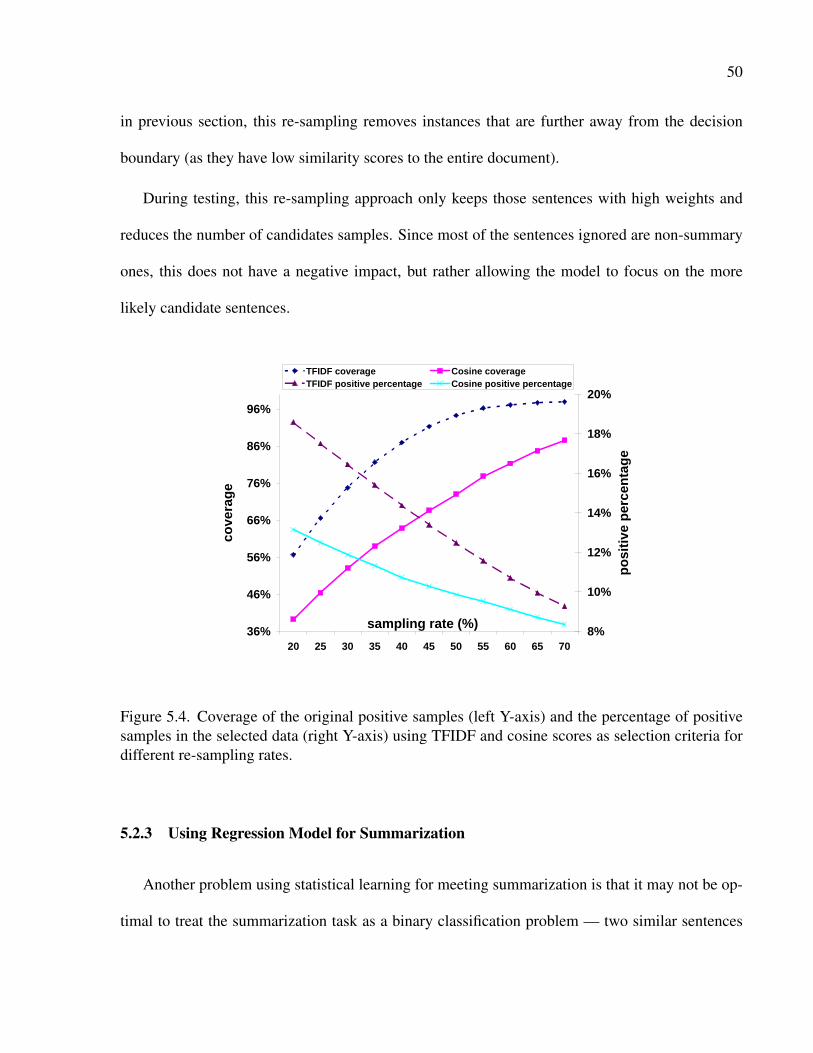
50
in previous section, this re-sampling removes instances that are further away from the decision
boundary (as they have low similarity scores to the entire document).
During testing, this re-sampling approach only keeps those sentences with high weights and
reduces the number of candidates samples. Since most of the sentences ignored are non-summary
ones, this does not have a negative impact, but rather allowing the model to focus on the more
likely candidate sentences.
36%
46%
56%
66%
76%
86%
96%
20 25 30 35 40 45 50 55 60 65 70
sampling rate (%)
cove
rage
8%
10%
12%
14%
16%
18%
20%
posi
tive
perc
enta
ge
TFIDF coverage Cosine coverageTFIDF positive percentage Cosine positive percentage
Figure 5.4. Coverage of the original positive samples (left Y-axis) and the percentage of positivesamples in the selected data (right Y-axis) using TFIDF and cosine scores as selection criteria fordifferent re-sampling rates.
5.2.3 Using Regression Model for Summarization
Another problem using statistical learning for meeting summarization is that it may not be op-
timal to treat the summarization task as a binary classification problem — two similar sentences

51
may be annotated with two different labels because of the preference by different annotators or
the need to avoid redundancy for summary selection or other reasons, as shown in the example
in Table 5.4. With such kind of confusion it may be hard for the model to learn to separate sum-
mary and non-summary sentences. Therefore, instead of using binary labels, we hypothesize that
the summarization task can be modeled as a regression problem, where the labels are numerical
numbers representing the importance of the sentences. We expect that the fine-grained weights
can provide more information of each sentence’s significance and help train a more discriminative
model.
The idea of assigning salience weight for the training instances is similar to the weighting
methods we used for up-sampling and down-sampling. We keep the label 1 for the summary sen-
tences, and compute target labels for those non-summary sentences using the same 6 weighting
measures listed in Table 5.5. Table 5.6 shows the numerical labels using cosine max for the ex-
ample sentences used in Table 5.4. The non-summary sentence has a negative label originally, but
now is assigned a high target label because of its similarity to the reference summary sentence.
For comparison, we also include the labels for this same example using up-sampling (changed to
positive) and down-sampling (this instance is removed).
Table 5.6. Example of new labels using regression, up-sampling, and down-sampling for a non-summary sentence (second row) that is similar to a summary sentence (first row).
Sentence original regression up-sampling down-samplingi think for word-level this would be ok. 1 1.0 1 1for word-level it’s alright. -1 0.968 1 removed
Once the target labels are assigned to all the training instances, we will use a regression model

52
to learn the underlying function to estimate the target labels. Regression analysis is a statistical tool
for investigating relationships between variables. A simple regression model is linear regression
that makes the prediction of one variable based on the knowledge of another one when there is
a statistically significant correlation between the two variables [68]. Another regression model is
logistic regression, which is used for predicting the probability of occurrence of an event by fitting
data to a logistic curve [69]. This model can be used as a classifier too, where during training, the
instances have two classes, and during testing, the model provides a posterior probability of the
membership of the test instance. However, our approach here is to use actual target label for each
training instances rather than the original binary labels.
The Support Vector Regression is the regression model we use in this work [70]. Similar
to SVM for binary classification, the goal of SVR is to find a function f(x) that has at most ε
deviation from the actual targets yi for all the training instances xi, and at the same time is as flat
as possible. Our preliminary experiments showed that SVR outperformed the logistic regression or
neural network. During testing, a regression score is predicted for each testing sample, then we use
the same method as in the classification approach to select the sentences based on their confidence
scores.
5.2.4 Forward Feature Selection
No matter which model we use for the summarization task, whether it is binary classification or
regression, the training and testing samples are represented by the feature set described in Section
5.1. In our study, we use forward feature selection (FFS) [71] to analyze the importance of different
features. The algorithm of FFS is shown below in Algorithm 1. It is a greedy algorithm. In every

53
iteration step, the best feature is selected when its addition to the current feature subset leads to the
greatest performance improvement.
Algorithm 1 Algorithm for Forward Feature Selection
Let P = Ø be the current set of selected featuresLet Q be the full set of featureswhile size of P is smaller than a given constant do
(a) for each v ∈ QSet P ′ ← P ∪ {v}Train the model with P ′ and evaluate on the dev set(b) Set P ← P ∪ {v∗}where v∗ is the the best feature obtained in step (a)(c) Set Q← Q\{v∗}(d) Record performance using current P
end while
5.3 Experimental Results and Discussion
5.3.1 Baseline Results
We provide two baseline results for comparison. The first one generates a summary by selecting
the longest sentences until reaching the specified length. The second one is the supervised approach
that selects the sentences with high confidence scores predicted by the SVM model using all the
features we described in Section 5.1. We provide results for a few different compression ratios
varying from 13% to 18%.
Table 5.7. ROUGE-1 F-measure results (%) of the baselines using human transcripts.
compression ratio 13% 14% 15% 16% 17% 18%Long sent selection 52.38 54.50 56.16 57.47 58.58 59.23
All features 67.25 67.80 67.76 67.56 67.22 66.86

54
Table 5.8. ROUGE-1 F-measure results (%) of the baselines using ASR outputs.
compression ratio 13% 14% 15% 16% 17% 18%Long sent selection 62.13 63.11 64.01 64.72 64.65 64.89
All features 62.05 63.35 64.24 64.64 64.77 64.38
Table 5.7 and Table 5.8 show the ROUGE-1 F-scores for the two baseline systems on the dev set
using the human transcripts and ASR output, respectively. Using sentence length to select summary
yields worse performance than using the classification approach on the human transcript condition;
however, the two systems achieve similar results on the ASR output. This finding is consistent with
the results reported in [39]. Comparing the performance on the human transcripts and ASR output
using classification approach, we see that the results are consistently better for human transcripts
on different compression ratios, which is expected. We can also compare the scores with the ones
in Table 4.3 obtained using the unsupervised approaches, MMR and the concept-based framework,
introduced in Section 4.2.3. This supervised baseline outperforms the MMR method, and achieved
comparable results as the concept-based one when using human transcripts. Overall, the baseline
results are very competitive with the previous work [13, 34, 39]. For the following experiments,
we use the results achieved by using the SVM classifier with all the features as the baseline, and
evaluate the performance improvement using our proposed approaches.
5.3.2 Results Using Sampling Methods
Since our focus here is on the approaches to deal with the imbalanced data problem, we fix the
word compression ratio and evaluate the effect of different sampling rates and weighting methods
on summarization performance using the development set. We use 14% and 17% word compres-

55
sion ratio for the human transcript and ASR outputs respectively. These compression ratios are
chosen based on the baseline results above.
Experimental Results Using Up-Sampling
Up-sampling is achieved by changing the labels of some negative instances to positive. These
negative instances are selected based on their similarity to the positive samples. In Section 5.2.2,
we described 6 weighting methods to assign scores to the negative instances for up-sampling, 3
based on cosine similarity, and the other 3 using ROUGE scores. Figure 5.5 shows the ROUGE-1
F-scores using the 6 weighting methods and different up-sampling rates on the human transcript
for the development set. The X-axis, the sampling rate, is the rate of the current positive sam-
ples to the original positive instances. When it is 1, none of the negative instances is changed
to positive and there are no newly added positive samples, that is, the results are the same as the
baseline system. We can see that different similarity measures and up-sampling ratios have great
influence on the system performance. Of all the weighting methods, the best results are obtained
using ROUGE mean and increasing the positive samples to 1.5 times of the original number. Com-
pared to the baseline result, up-sampling yields an improvement from 67.80% to 69.24%. Using
the similarity measure ROUGE mean, the performance improves when we change more negative
instances to positive until the sampling ratio reaches 1.5. After that, increasing the up-sampling
ratio leads to performance drop. But for other similarity measures, the trend is not clear — the
results are more random and there is more fluctuation.
The results for the ASR condition are shown in Figure 5.6. The same setting, ROUGE mean
and 1.5 up-sampling rate, also outperforms the baseline result (65.66% vs. 64.77%). However,

56
0.54
0.56
0.58
0.60
0.62
0.64
0.66
0.68
0.70
1 1.2 1.5 1.8 2 3 4
sampling rate
RO
UG
E-1
F-sc
ore
Cosine_max mean all ROUGE_max mean all
Figure 5.5. ROUGE-1 F-measure results (%) using up-sampling on human transcripts.
using the weighting measure Cosine mean and a sampling rate of 4, achieves slightly better result,
65.97%. But the pattern using different sampling rates for the Cosine mean similarity measure is
not as clear as for ROUGE mean. Comparing ASR and human transcripts, it seems that a higher
up-sampling rate is often preferred for ASR output and there is more fluctuation in the human
transcript condition when varying the sampling rates.
Our proposed up-sampling approach is different from commonly used up-sampling method
that replicates the samples in the minority class, therefore next we evaluate the performance of up-
sampling by varying the number of times that we replicate the summary sentences. The ROUGE-1
F-measure results from these experiments are shown in Table 5.9 using the human transcripts and
ASR output respectively. When the up-sampling rate is 1, it is the same as the baseline setup. For
human transcripts, replicating the positive class degraded performance; in contrast, our proposed
up-sampling method can yield performance gain. When using ASR output, for some upsampling

57
0.62
0.63
0.64
0.65
0.66
1 1.2 1.5 1.8 2 3 4
sampling rate
RO
UG
E-1
F-sc
ore
Cosine_max mean all ROUGE_max mean all
Figure 5.6. ROUGE-1 F-measure results (%) using up-sampling on ASR outputs.
rates, there is an improvement. The best result is similar to that in our proposed up-sampling
method. However, there can also be significant performance drop for some up-sampling rates.
Compared to our approach above, the performance variance when changing the up-sampling rates
seems to be greater when up-sampling is achieved by replicating minority samples. Overall, for all
the up-sampling approaches, there is not a consistent correlation between the system performance
and how balanced the resulting data set is after up-sampling.
Table 5.9. ROUGE-1 F-measure results (%) of up-sampling by replicating the positive samples onboth human transcripts and ASR outputs.
Up-sampling rate 1 2 3 4 5 6Human 67.80 63.73 57.39 55.18 57.89 58.36ASR 64.77 59.94 66.18 65.57 65.49 66.04

58
Experimental Results Using Down-Sampling
The same weighting methods are used for down-sampling, with the goal of removing nega-
tive instances with high similarity scores to the summary sentences. Figure 5.7 shows the down-
sampling results on the development set using human transcripts. The X-axis, the down-sampling
rate, represents the percentage of the removed negative instances. When it is 0, it means that no
negative instances are removed, which is the baseline setup. We see from the results that the best
performance is obtained using ROUGE mean as the weighting method with a down-sampling rate
of 5%. The performance is improved from 67.80% to 70.28%. The experimental results on the
ASR outputs are shown in Figure 5.8. Using the same weighting method and down-sampling rate,
we obtain the best score for ASR outputs, 66.42% compared to the baseline score of 64.77%. For
this similarity measure ROUGE mean, we observe that the best result is achieved with a sampling
rate of 5%, then the performance starts degrading when removing more instances from the data
set. This observation is consistent for the human transcripts and ASR output.
In up-sampling and down-sampling, for most of the experiments, ROUGE mean outperforms
the other weighting measures, except for up-sampling on ASR output, where Cosine mean is
slightly better. This is consistent with our expectation that ROUGE is the final evaluation met-
ric, and is expected to be a better weighting method for capturing the sentence similarity. The best
scores are obtained by the mean value of the weighting methods, which suggests that the selected
sentences should be the most similar ones to the entire summary, not to a specific sentence (as is
done using the max value). In addition, the fact that the average of the cosine similarity or ROUGE
scores yields better performance indicates that it is better to give equal weight to different summary
sentences than more weight to longer sentences.

59
0.55
0.57
0.59
0.61
0.63
0.65
0.67
0.69
0.71
0% 5% 10% 15% 20% 25% 30%
sampling rate
RO
UG
E-1
F-sc
ore
Cosine_max mean all ROUGE_max mean all
Figure 5.7. ROUGE-1 F-measure results (%) using down-sampling on human transcripts.
0.63
0.64
0.65
0.66
0.67
0% 5% 10% 15% 20% 25% 30%sampling rate
RO
UG
E-1
F-sc
ore
Cosine_max mean all ROUGE_max mean all
Figure 5.8. ROUGE-1 F-measure results (%) using down-sampling on ASR outputs.

60
For a comparison with the down-sampling approach above, we also evaluate a commonly used
down-sampling method, e.g., randomly removing the negative samples from the data set. Because
the removed samples are randomly selected, we performed three random sampling and obtained
the average results of the three runs. Table 5.10 shows the ROUGE-1 results for human transcripts
and ASR output respectively when varying the down-sampling rates. Using the human transcripts,
there is only marginal change of the results for different sampling rates. The results on ASR output
fluctuate for different sampling rates. There is performance gain for a few different setups. Our
proposed approach outperforms this commonly used down-sampling method for both human tran-
scripts and ASR condition. In addition, our approach has similar patterns on the human transcripts
and ASR output, whereas this down-sampling by random selection has a different trend for these
two conditions.
Table 5.10. ROUGE-1 F-measure Results (%) of down-sampling by randomly removing negativesamples on both human transcripts and ASR output.
Down-sampling rate (%) 5 10 15 20 25 30Human 68.53 67.86 67.86 68.34 68.33 68.00ASR 64.74 65.30 64.31 65.35 66.10 64.52
Experimental Results Using Re-Sampling
For re-sampling, we use different selection criteria to retain some training and test instances.
We compare two measurements: TFIDF and cosine similarity, as introduced in Section 5.2.2. Fig-
ure 5.9 shows the re-sampling results on human transcripts and ASR outputs for the development
set. The X-axis, re-sampling rate, is the percentage of the instances preserved. When it is 100%,
we do not delete any instances, so the results are the same as the baseline. For human transcripts,

61
we notice that when using cosine similarity scores to keep the top 20% instances, we obtain the
best score of 70.41%. The sampling rate is relatively low (20%), which results in an average pos-
itive coverage of 39.3% on the training set. This implies that the positive coverage is not the only
criteria to evaluate a weighting method for re-sampling. The system performance is also dependent
on which sentences are actually preserved by this weighting method, for both positive and negative
classes. From the results on ASR outputs, we observe very different patterns. The best score on
ASR outputs is obtained using TFIDF as the selection metric, and keeping the top 35% samples.
This yields a performance improvement from 64.77% to 66.27%.
0.67
0.68
0.69
0.7
0.71
20% 25% 30% 35% 40% 45% 50% 100%
sampling rate
RO
UG
E-1
F-sc
ore
TFIDF Cosine
(a) on human transcripts
0.62
0.63
0.64
0.65
0.66
0.67
20% 25% 30% 35% 40% 45% 50% 100%
sampling rate
RO
UG
E-1
F-sc
ore
TFIDF Cosine
(b) on ASR outputs
Figure 5.9. ROUGE-1 F-measure results (%) using the re-sampling method.
5.3.3 Regression Results
To use the regression model, we need continuous labels for the training instances. These tar-
get labels are generated using the same weighting methods as used for up-sampling and down-
sampling. The regression results on human transcripts and ASR outputs are shown in Figure 5.10
for different word compression ratios. The baseline result is from the binary classification sys-

62
tem using all the features. Here we only present results for the best weighting measure using
cosine similarity and ROUGE. Using human transcripts, we notice that the results of cosine-based
weighting methods are worse than the baseline system, however, using ROUGE-based weight-
ing, we obtain better performance, for example, 69.23% for the word compression ratio of 14%.
The patterns for ASR outputs are different from the human transcripts. Cosine-based weighting is
superior to ROUGE-based measures, and both achieve better performance than the baseline.
0.63
0.64
0.65
0.66
0.67
0.68
0.69
0.70
13% 14% 15% 16% 17% 18%
word compression ratio
RO
UG
E-1
F-sc
ore
baseline Cosine_ALL ROUGE_MAX
(a) on human transcripts
0.60
0.61
0.62
0.63
0.64
0.65
0.66
0.67
13% 14% 15% 16% 17% 18%
word compression ratio
RO
UG
E-1
F-sc
ore
baseline Cosine_MEAN ROUGE_ALL
(b) on ASR outputs
Figure 5.10. ROUGE-1 F-measure results (%) using the regression model.
Then we evaluate the feasibility of combining regression and sampling approaches. For each
sampled instance, we change its binary label to a continuous number in order to use a regression
model for training and testing. Since the up-sampling approach selects a negative sentence and
changes its label to positive, when assigning continuous weights for each instance, there is no
difference with just using the regression setup itself. However, for down-sampling and re-sampling
methods, the results are different because some of the instances are removed from the corpus.
Therefore we only combine regression with down-sampling and re-sampling. Table 5.11 shows
the combination results, along with using each method alone. We observe that combining these

63
two methods can not yield further improvement. This is probably because the sampling methods
are proposed mainly to deal with the imbalanced data problem, which does not exist in regression
model. The labels of the instances in regression are numerical numbers, and the summarization
task is solved using a regression model instead of a binary classification model.
Table 5.11. ROUGE-1 F-measure results (%) of combining sampling and regression. ‘Ds’ isdown-sampling; ‘Rs’ is re-sampling; ‘Rg’ is regression.
baseline Ds Rs Rg Rg&Ds Rg&RsHuman 67.80 70.28 70.41 69.23 68.99 69.04ASR 64.77 66.42 66.27 66.59 66.56 66.56
5.3.4 Feature Selection Results
All the instances in previous experiments are represented by the features described in Sec-
tion 5.1. In order to analyze the effectiveness of different feature subsets, we use the forward
feature selection (FFS) algorithm in Section 5.2.4 to rank each feature.
Features Selected Using FFS
We run forward feature selection on the development set. The original data set (i.e., without
any sampling or regression) is used first to select features. Instead of using classification accuracy
or error rate, we use the ROUGE score (ROUGE-1 F-measure) as the selection criterion, since
that is our ultimate performance measure. We train an SVM model, and predict each sentence’s
confidence score of being in the summary on the development set. The summary is extracted by
selecting the sentences with the highest probabilities, with a word compression ratio of 14% for
human transcripts, and 17% for ASR output.

64
The top features selected incrementally by FFS for human transcripts are listed in Table 5.12,
along with the ROUGE-1 F-measure score after adding each feature iteratively. The score when
using all the features is also shown in the table for a comparison. The results show that a subset
of the features can outperform using all the features, therefore feature selection is important for
this task. The sentence length is selected as the top feature, which also validates our choice of the
baseline system by selecting long sentences. The frequent unigram, bigram and the first appearing
noun and pronoun are also included in the top features, which shows that the lexical cues are very
predictive in the domain of meeting summarization. Different TF-IDF related features, such as IDF
I and II, TF III, TFIDF II and III, prove to be very helpful for summarization, which is consistent
with the previous research [34, 56, 63]. In addition, feature SUIDF III, representing the term usage
in different speakers suggested in [56], also proves to be useful for this task.
Table 5.12. ROUGE-1 F-measure results (%) after Forward Feature Selection for human tran-scripts.
Feature Feature Description ROUGEBigram most frequent bigram 68.92+ IDF I Mean of IDF 70.12
+ TFIDF II Max of TFIDF 70.67+ Noun II # of first appearing noun in current sentence 70.18
+Len I previous sentence length 69.91+Unigram most frequent words 69.85+ IDF II Max of IDF 70.49+Len II current sentence length 71.09
+ Noun I # of first appearing noun in previous sentence 71.35+ TF III Sum of TF 71.45
+ SUIDF III Sum of SUIDF 71.09+ Noun III # of first appearing noun in next sentence 70.85+ Cosine cosine similarity score 70.85
+ TFIDF III Sum of TFIDF 71.18+ Pronoun II # of first appearing pronoun in current sentence 71.55All features 67.80
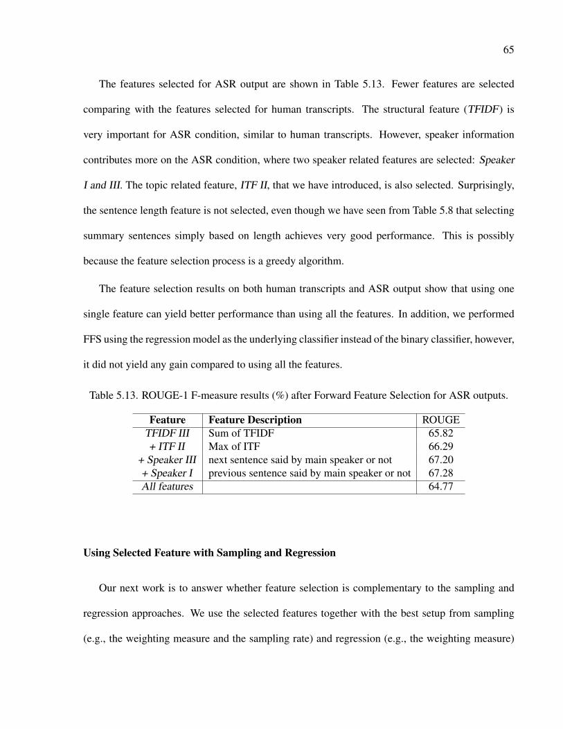
65
The features selected for ASR output are shown in Table 5.13. Fewer features are selected
comparing with the features selected for human transcripts. The structural feature (TFIDF ) is
very important for ASR condition, similar to human transcripts. However, speaker information
contributes more on the ASR condition, where two speaker related features are selected: Speaker
I and III. The topic related feature, ITF II, that we have introduced, is also selected. Surprisingly,
the sentence length feature is not selected, even though we have seen from Table 5.8 that selecting
summary sentences simply based on length achieves very good performance. This is possibly
because the feature selection process is a greedy algorithm.
The feature selection results on both human transcripts and ASR output show that using one
single feature can yield better performance than using all the features. In addition, we performed
FFS using the regression model as the underlying classifier instead of the binary classifier, however,
it did not yield any gain compared to using all the features.
Table 5.13. ROUGE-1 F-measure results (%) after Forward Feature Selection for ASR outputs.
Feature Feature Description ROUGETFIDF III Sum of TFIDF 65.82+ ITF II Max of ITF 66.29
+ Speaker III next sentence said by main speaker or not 67.20+ Speaker I previous sentence said by main speaker or not 67.28All features 64.77
Using Selected Feature with Sampling and Regression
Our next work is to answer whether feature selection is complementary to the sampling and
regression approaches. We use the selected features together with the best setup from sampling
(e.g., the weighting measure and the sampling rate) and regression (e.g., the weighting measure)
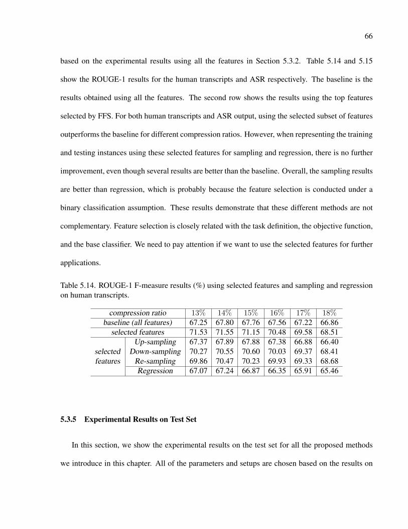
66
based on the experimental results using all the features in Section 5.3.2. Table 5.14 and 5.15
show the ROUGE-1 results for the human transcripts and ASR respectively. The baseline is the
results obtained using all the features. The second row shows the results using the top features
selected by FFS. For both human transcripts and ASR output, using the selected subset of features
outperforms the baseline for different compression ratios. However, when representing the training
and testing instances using these selected features for sampling and regression, there is no further
improvement, even though several results are better than the baseline. Overall, the sampling results
are better than regression, which is probably because the feature selection is conducted under a
binary classification assumption. These results demonstrate that these different methods are not
complementary. Feature selection is closely related with the task definition, the objective function,
and the base classifier. We need to pay attention if we want to use the selected features for further
applications.
Table 5.14. ROUGE-1 F-measure results (%) using selected features and sampling and regressionon human transcripts.
compression ratio 13% 14% 15% 16% 17% 18%baseline (all features) 67.25 67.80 67.76 67.56 67.22 66.86
selected features 71.53 71.55 71.15 70.48 69.58 68.51Up-sampling 67.37 67.89 67.88 67.38 66.88 66.40
selected Down-sampling 70.27 70.55 70.60 70.03 69.37 68.41features Re-sampling 69.86 70.47 70.23 69.93 69.33 68.68
Regression 67.07 67.24 66.87 66.35 65.91 65.46
5.3.5 Experimental Results on Test Set
In this section, we show the experimental results on the test set for all the proposed methods
we introduce in this chapter. All of the parameters and setups are chosen based on the results on
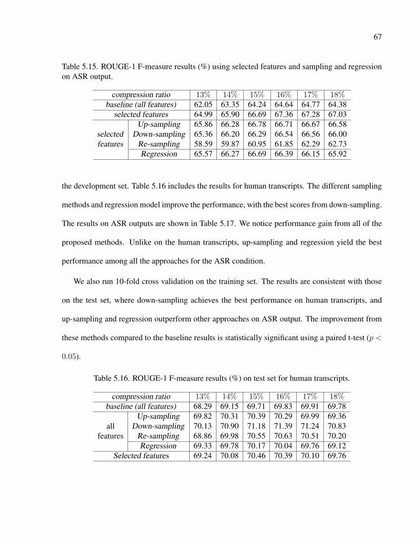
67
Table 5.15. ROUGE-1 F-measure results (%) using selected features and sampling and regressionon ASR output.
compression ratio 13% 14% 15% 16% 17% 18%baseline (all features) 62.05 63.35 64.24 64.64 64.77 64.38
selected features 64.99 65.90 66.69 67.36 67.28 67.03Up-sampling 65.86 66.28 66.78 66.71 66.67 66.58
selected Down-sampling 65.36 66.20 66.29 66.54 66.56 66.00features Re-sampling 58.59 59.87 60.95 61.85 62.29 62.73
Regression 65.57 66.27 66.69 66.39 66.15 65.92
the development set. Table 5.16 includes the results for human transcripts. The different sampling
methods and regression model improve the performance, with the best scores from down-sampling.
The results on ASR outputs are shown in Table 5.17. We notice performance gain from all of the
proposed methods. Unlike on the human transcripts, up-sampling and regression yield the best
performance among all the approaches for the ASR condition.
We also run 10-fold cross validation on the training set. The results are consistent with those
on the test set, where down-sampling achieves the best performance on human transcripts, and
up-sampling and regression outperform other approaches on ASR output. The improvement from
these methods compared to the baseline results is statistically significant using a paired t-test (p <
0.05).
Table 5.16. ROUGE-1 F-measure results (%) on test set for human transcripts.
compression ratio 13% 14% 15% 16% 17% 18%baseline (all features) 68.29 69.15 69.71 69.83 69.91 69.78
Up-sampling 69.82 70.31 70.39 70.29 69.99 69.36all Down-sampling 70.13 70.90 71.18 71.39 71.24 70.83
features Re-sampling 68.86 69.98 70.55 70.63 70.51 70.20Regression 69.33 69.78 70.17 70.04 69.76 69.12
Selected features 69.24 70.08 70.46 70.39 70.10 69.76
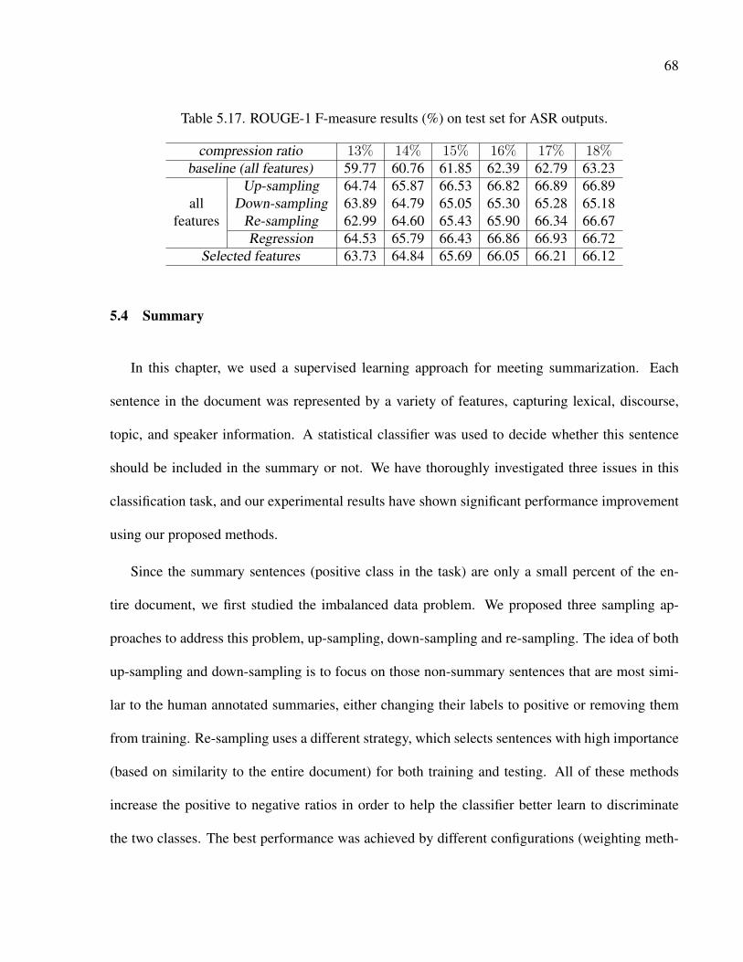
68
Table 5.17. ROUGE-1 F-measure results (%) on test set for ASR outputs.
compression ratio 13% 14% 15% 16% 17% 18%baseline (all features) 59.77 60.76 61.85 62.39 62.79 63.23
Up-sampling 64.74 65.87 66.53 66.82 66.89 66.89all Down-sampling 63.89 64.79 65.05 65.30 65.28 65.18
features Re-sampling 62.99 64.60 65.43 65.90 66.34 66.67Regression 64.53 65.79 66.43 66.86 66.93 66.72
Selected features 63.73 64.84 65.69 66.05 66.21 66.12
5.4 Summary
In this chapter, we used a supervised learning approach for meeting summarization. Each
sentence in the document was represented by a variety of features, capturing lexical, discourse,
topic, and speaker information. A statistical classifier was used to decide whether this sentence
should be included in the summary or not. We have thoroughly investigated three issues in this
classification task, and our experimental results have shown significant performance improvement
using our proposed methods.
Since the summary sentences (positive class in the task) are only a small percent of the en-
tire document, we first studied the imbalanced data problem. We proposed three sampling ap-
proaches to address this problem, up-sampling, down-sampling and re-sampling. The idea of both
up-sampling and down-sampling is to focus on those non-summary sentences that are most simi-
lar to the human annotated summaries, either changing their labels to positive or removing them
from training. Re-sampling uses a different strategy, which selects sentences with high importance
(based on similarity to the entire document) for both training and testing. All of these methods
increase the positive to negative ratios in order to help the classifier better learn to discriminate
the two classes. The best performance was achieved by different configurations (weighting meth-

69
ods and sampling rates), but overall, we have observed consistent performance gain using these
sampling methods on both human transcripts and ASR conditions.
Second we investigated using a regression model rather than binary classification for this task.
Each training sentence was assigned a numerical weight according to its similarity to the annotated
summary sentences. These new labels of the training samples represent fine grained information,
and take into account human annotation disagreement. Our experimental results showed this re-
gression model is quite robust and outperforms the binary classification setup.
Last we used forward feature selection to evaluate the contribution of various features used for
meeting summarization. We selected a subset of important features for human transcripts and ASR
outputs respectively. Our analysis showed that the structural features are very important for both
human transcripts and ASR outputs. The lexical features are more indicative for human transcripts,
whereas for ASR outputs, the speaker related features are used more heavily. Our results have
shown that using the subset of the features yielded better performance than using the entire feature
set, especially for the ASR condition on the test set. However, when we used these selected features
as the representation of each instance and combined with the sampling and regression approaches,
there is no further improvement. We will investigate how to effectively combine these different
approaches in our future work.

CHAPTER 6
FROM TEXT TO SPEECH SUMMARIZATION ∗
The methods we introduced in previous chapters can be applied to both text and speech sum-
marization, since we do not use any speech specific information. In this chapter we investigate
using speech information to improve the speech summarization performance, and addressing the
problems caused by ASR errors.
Previous work has shown that combing acoustic/prosodic features with traditional textual fea-
tures can further improve the summarization performance for some speech domains, such as broad-
cast news and lectures. Less analysis has been conducted for meeting summarization. So far most
of meeting summarization research using supervised learning has focused on lexical and structural
features, such as [32]. In this chapter, we will analyze the effectiveness of prosodic features, aim-
ing to answer the question how they can be more effectively used for meeting summarization, and
whether it is possible to construct a good text-independent summarizer by only using the prosodic
features. Furthermore, since the acoustic and textual features can be considered as conditionally
independent, we will investigate using co-training algorithm to increase the classification accuracy
by leveraging the information from a large amount of unlabeled data.
In the experimental results shown in previous chapters, we find that the performance using the
ASR output is consistently lower (to different extent) comparing to that using human transcripts no
∗ c© 2010 IEEE. Reprinted, with permission, from IEEE Transactions on Audio, Speech and Language Processing,
Using N-best Lists and Confusion Networks for Meeting Summarization, Shasha Xie and Yang Liu
70

71
matter whether supervised or unsupervised approaches were used. To address the problem caused
by imperfect recognition transcripts, in this chapter we will also investigate using rich speech
recognition results for summarization.
6.1 Integrating Prosodic Features in Extractive Meeting Summarization †
Compared to text summarization that relies on lexical, syntactic, positional and structural in-
formation, speech summarization can leverage the additional sources of information contained in
speech, such as speaker and acoustic/prosodic information. These provide important information
for summarization as they represent how a sentence is said other than what it is said. Several
recent studies have evaluated the impact of traditional textual features and speech-specific acous-
tic/prosodic features using classifier-based methods in speech summarization [12, 33, 35, 39, 72].
For the broadcast news domain, [33, 35] showed that the best performance was obtained by com-
bining acoustic features with lexical, structural and discourse features; however, using only acous-
tic and structural features can achieve good performance when speech transcription is not avail-
able. Similar findings are also presented in [72] using acoustic and structural features for Mandarin
broadcast news. In contrast, [12] showed different patterns for lecture summarization than broad-
cast news domain. The acoustic and structural features are less important due to the fact that the
speaking styles of anchors and reporters are relatively consistent in broadcast news, whereas the
speaking styles of lecture speakers vary a lot. In this section, we analyze the effectiveness of
prosodic features, aiming to answer the question how they can be more effectively used for meet-
ing summarization, and whether it is possible to construct a good text-independent summarizer by
only using the prosodic features.
†Joint work with Dilek Hakkani-Tur and Benoit Favre

72
6.1.1 Acoustic/Prosodic Features
Following previous research on speech summarization, we first extract 13 original features
using Praat [73]. We have five F0 related features representing the minimum, maximum, median,
mean value of F0, and the range of F0 for each instance. Similarly, we extract five energy features
also for the minimum, maximum, median, mean value of energy, and the range of energy of each
sample. We include a duration feature which is the length of the sentence in seconds. Two speaking
rate features are used, which are the sentence duration divided by the number of words and the
number of letters in each sentence, respectively.
For these prosodic features, in addition to the raw values, we investigate different normalization
methods based on various information.
• Speaker-based normalization
Meeting recordings have multiple speakers. In general, speakers have different pitch, energy
and speaking rates. In this normalization measure, each of the feature values is normalized
using the mean and variance values of that feature for each speaker.
• Topic-based normalization
Meetings can often be divided into several parts, each with its own topic based on the dis-
cussion. We assume that a speaker may have different prosodic behaviors for different topics
according to his/her interest, roles, or conversation partners in a topic discussion. Therefore
in this method, all the feature values are normalized using the mean and variance values for
a topic. Note that this normalization is performed for each speaker.
• Local window-based normalization

73
This method does not rely on content information like the topic-based normalization or use
only the information from the speaker himself. We expect that the speakers are affected by
other participants and may adjust their speaking rates, pitch, or energy according to who they
are talking to in a local context. We simply use the previous and the following N instances
to normalize the feature values.
Following the idea of local window normalization, we expect that the differences between
the current sentence and its neighbors in terms of prosodic cues can indicate the importance of
the current sentence, therefore we propose to include prosodic delta features — the difference
between the current instance’s feature values to its previous M and next M instances. The idea of
computing delta features has been widely used in tasks such as speech and speaker recognition to
represent dynamic information.
6.1.2 Experiments
We first present experimental results for the development set to evaluate various factors, includ-
ing prosodic feature normalization methods, effect of prosodic delta features, and combination of
prosodic and non-prosodic features. Then we demonstrate the final results on the test set.
Baseline Results
The baseline in our experiments is using all the non-prosodic features we described in Section
5.1.1. Table 6.1 shows the ROUGE-1 (unigram match) F-measure scores for the human transcripts
and ASR output. For the ASR condition, all the non-prosodic features are extracted from the ASR
transcripts for both training and testing.
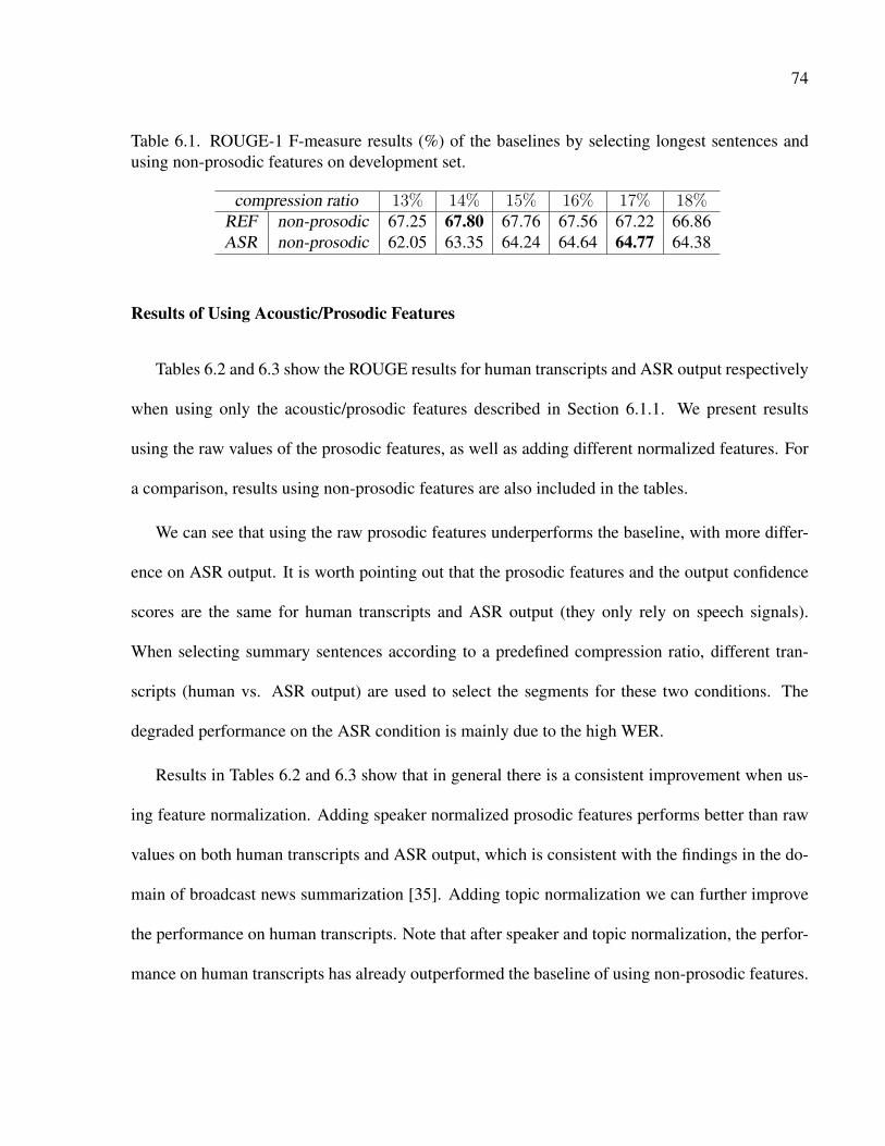
74
Table 6.1. ROUGE-1 F-measure results (%) of the baselines by selecting longest sentences andusing non-prosodic features on development set.
compression ratio 13% 14% 15% 16% 17% 18%REF non-prosodic 67.25 67.80 67.76 67.56 67.22 66.86ASR non-prosodic 62.05 63.35 64.24 64.64 64.77 64.38
Results of Using Acoustic/Prosodic Features
Tables 6.2 and 6.3 show the ROUGE results for human transcripts and ASR output respectively
when using only the acoustic/prosodic features described in Section 6.1.1. We present results
using the raw values of the prosodic features, as well as adding different normalized features. For
a comparison, results using non-prosodic features are also included in the tables.
We can see that using the raw prosodic features underperforms the baseline, with more differ-
ence on ASR output. It is worth pointing out that the prosodic features and the output confidence
scores are the same for human transcripts and ASR output (they only rely on speech signals).
When selecting summary sentences according to a predefined compression ratio, different tran-
scripts (human vs. ASR output) are used to select the segments for these two conditions. The
degraded performance on the ASR condition is mainly due to the high WER.
Results in Tables 6.2 and 6.3 show that in general there is a consistent improvement when us-
ing feature normalization. Adding speaker normalized prosodic features performs better than raw
values on both human transcripts and ASR output, which is consistent with the findings in the do-
main of broadcast news summarization [35]. Adding topic normalization we can further improve
the performance on human transcripts. Note that after speaker and topic normalization, the perfor-
mance on human transcripts has already outperformed the baseline of using non-prosodic features.

75
Table 6.2. ROUGE-1 F-measure results (%) using raw values and different normalization methodsof acoustic/prosodic features on development set for human transcripts.
ratio baselineprosodic features
raw valuewith normalization
speaker speaker & topic window13% 67.25 65.74 65.75 67.53 67.6514% 67.80 66.13 66.35 68.08 68.2515% 67.76 66.42 66.84 68.40 69.0116% 67.56 66.14 66.91 68.25 69.0317% 67.22 65.78 67.09 68.20 68.6318% 66.86 65.42 66.96 67.71 68.35
Table 6.3. ROUGE-1 F-measure results (%) using raw values and different normalization methodsof acoustic/prosodic features on development set for ASR output.
ratio baselineprosodic features
raw valuewith normalization
speaker speaker & topic window13% 62.05 59.54 60.07 59.62 62.5114% 63.35 60.75 61.61 60.78 63.5815% 64.24 61.59 62.55 61.73 64.4616% 64.64 62.12 63.39 62.19 65.0217% 64.77 62.37 63.55 62.31 65.6218% 64.38 62.56 63.84 62.22 65.63

76
However, for ASR condition, adding topic information degrades the ROUGE scores. That’s prob-
ably because the speech recognition accuracy is different for each topic. The local window based
normalization is the most effective one among these three normalization methods for both human
transcripts and ASR output. We try different window length for human transcripts and ASR output
respectively. The best window size for human transcripts is half of the document length, but for
ASR output a smaller window is assigned (1/9 of the document size). This normalization method
yields a significantly better score than the baseline (69.03 vs. 67.56) on human transcripts, but the
difference on ASR output is much less.
Although using the raw values of prosodic features does not perform as well as using non-
prosodic features, we can see that with proper normalization, we obtain better performance than
the baseline using the non-prosodic features. This shows the feasibility of extracting the summary
without text information. Because the worse performance on ASR output is mainly caused by the
WER, the performance drop when using ASR output indicates that the selected summary sentences
have recognition errors. [13] showed that summary sentences have lower WER than the average
WER. But we can still see the WER has a great influence on summarization performance for the
meeting domain.
The experimental results of adding the delta features are shown in Table 6.4 using the best
normalization setup (local window normalization). The delta features are the difference between
the current instance’s feature values and its previous and next M instances. We also try different
M values, and the best one is 4 for human trnascripts and 5 for ASR output. We notice that
adding the prosodic differences substantially improves the performance, with more gain on human
transcripts than ASR output. Comparing with the results presented in previous work using a large

77
set of features including lexical, structural, discourse and prosodic features [13, 34, 74], we obtain
state-of-the-art results by only using the acoustic/prosodic features.
Table 6.4. ROUGE-1 F-measure results (%) of adding delta features on development set.
compression ratio 13% 14% 15% 16% 17% 18%REF window norm 67.65 68.25 69.01 69.03 68.63 68.35
+delta 69.9 70.8 71.18 71.18 70.69 70.49ASR window norm 62.51 63.58 64.46 65.02 65.62 65.63
+delta 63.42 64.65 65.78 66.07 66.31 66.31
To evaluate the effect of different prosodic features, we performed remove-one feature eval-
uation using human transcripts. In order to better understand the impact of the basic prosodic
features, in this experiment, we only used the raw prosodic features and their local window nor-
malized values. Furthermore, since the prosodic modeling part for human transcripts and ASR
output is the same, we use results on the human transcripts to avoid the confounding effect of ASR
errors in calculating the ROUGE scores. We list the five most and least effective features together
with their performance loss in Table 6.5. The ranking of the features is obtained based on the
performance change when removing the feature from the entire feature set.
Table 6.5. The five most and least effective prosodic features evaluated using human transcripts ondevelopment set.
Most Effective Features Less Effective FeaturesEnergy range (5.1%) f0 median (-0.3%)Normalized f0 median (4.7%) normalized energy mean (0.7%)energy mean (4.3%) speaking rate (letter) (0.7%)energy median (3.8%) normalized energy maximum (1.0%)f0 maximum (3.1%) normalized f0 mean (1.1%)
78
Combination with Non-prosodic Features
Finally we investigate if these prosodic features combine well with the non-prosodic features
to further improve the system performance. We use two different combination methods. First is
the feature level combination. We combine the non-prosodic features with the prosodic feature set
that yielded the best results (basic acoustic/prosodic features with local window normalization and
delta features) in one large feature set. The second one is a decision level combination. We train
separate models for these two information sources and then for each test instance linearly combine
the confidence scores from the two models. The final summary is constructed by selecting the
instances with higher combined confidence scores. The experimental results are presented in Table
6.6, along with the individual results using prosodic or non-prosodic information only. For the
decision level combination method, we varied the combination weights for human transcripts and
ASR output respectively, and show the best results here.
From the results, we can see that feature level combination hurts the summarization perfor-
mance compared to using one information source only, and there is more degradation on human
transcripts. However, we observe performance improvement using decision level combination for
both human transcripts and ASR output. Interestingly, we notice that for human transcripts, a
higher weight was given to the prosodic model (0.7 for prosodic and 0.3 for non-prosodic). This
is consistent with the individual model performance — the results of prosodic features are much
better than the non-prosodic ones. For ASR condition, equal weights (0.5 and 0.5) were used
for the two models, which can be explained in part by the fact that the two systems have similar
performance.

79
Table 6.6. ROUGE-1 F-measure results (%) of integrating prosodic and non-prosodic information,in comparison with using only one information source on development set.
compression ratio 13% 14% 15% 16% 17% 18%non-prosodic 67.25 67.80 67.76 67.56 67.22 66.86
REF prosodic 69.9 70.8 71.18 71.18 70.69 70.49feature combine 66.10 66.70 66.61 66.51 66.40 65.84
decision combine 70.50 70.92 71.40 70.91 70.67 70.18non-prosodic 62.05 63.35 64.24 64.64 64.77 64.38
ASR prosodic 63.42 64.65 65.78 66.07 66.31 66.31feature combine 63.06 64.16 64.75 65.40 65.44 65.23
decision combine 64.15 65.36 66.12 66.44 67.10 67.02
Results on Test Set
The results on the test set are provided in Table 6.7 for both human transcripts and ASR output,
using only non-prosodic or prosodic information, and their combination. ROUGE-2 scores (bigram
matching) are also included in order to provide more information for comparison. We selected the
best setup based on the results on the development set and applied it to the test set. The prosodic
feature set includes local window normalization and delta features. The combined system is based
on a decision level combination of the prosodic and non-prosodic models. We observe similar
trends as on the development set. Using only the prosodic features we obtain better performance
than non-prosodic information, and the combination of the models yields further improvement.
These results are consistent across human transcripts and ASR output, ROUGE-1 and ROUGE-2
scores. We also verified that the results are significantly better than the baseline according to a
paired t-test (p < 0.05).

80
Table 6.7. ROUGE-1 F-measure results (%) on test set.
ROUGE-1 F-measure ROUGE-2 F-measurecompression ratio 13% 14% 15% 16% 17% 18% 13% 14% 15% 16% 17% 18%
non-prosodic 68.29 69.15 69.71 69.83 69.91 69.78 33.29 34.05 34.51 35.10 35.61 36.14REF prosodic 68.87 69.85 70.28 70.56 70.36 69.86 36.14 37.51 38.07 39.03 39.10 39.23
combined 69.64 70.54 71.04 71.23 71.00 70.62 37.34 37.90 38.73 39.11 39.20 39.37non-prosodic 59.77 60.76 61.85 62.39 62.79 63.23 21.17 21.45 22.49 22.94 23.33 23.95
ASR prosodic 64.55 65.18 65.51 65.51 65.41 65.07 27.68 28.34 29.07 29.43 29.43 29.86combined 65.14 65.91 66.53 66.72 66.63 66.19 27.84 28.63 29.58 30.30 31.00 31.41
6.2 Semi-Supervised Extractive Speech Summarization via Co-Training Algorithm ‡
Although the experimental results in Chapter 4 and 5 showed that supervised learning ap-
proaches achieved better performance than unsupervised ones, learning a summarization classifier
requires a large amount of labeled data for training. Summary annotation is often difficult, ex-
pensive, and time consuming. Annotation of meeting recordings is especially hard because the
documents to be summarized are transcripts of natural meetings that have very spontaneous style,
contain many disfluencies, have multiple speakers, and are less coherent in content, and probably
have a lot of errors if the transcripts are from automatic speech recognition system. It is very hard
to read and understand the document, not to mention extracting the summary. On the contrary,
meeting recordings and their transcripts are relatively much easier to collect. This situation creates
a good opportunity for semi-supervised learning that can use large amount of unlabeled data, to-
gether with the labeled data, to build better classifiers. This technique has been shown to be very
promising in many speech and language processing tasks, such as question classification, web clas-
sification, word-sense disambiguation and prosodic event detection [75, 76, 77, 78]. In this section,
‡This is a joint work with Hui Lin.
81
we use the co-training algorithm [79] to explore semi-surprised learning in speech summarization.
Co-training assumes that features can be split into two sets, which are conditionally independent
given the class, and each of which is sufficient to train a good classifier. Unlike in text summariza-
tion task (where only textual information is available), we can easily extract two different views of
features for speech summarization: one from the textual transcripts, and the other from the speech
recordings§.
6.2.1 Co-Training Algorithm for Meeting Summarization
Co-training algorithm was introduced to increase the classification accuracy by exploiting the
information from a large amount of unlabeled data, together with a small set of labeled data [79].
Co-training assumes that the features can be split into two independent sets, and each set is suffi-
cient to train a good classifier. Initially two separate classifiers are trained with the labeled data,
on the two sub-feature sets respectively. Each classifier then classifies the unlabeled data, selects
the samples that they feel most confident with, and uses these automatically labeled samples along
with the original labeled data to “teach” the other classifier. This process iterates until the classifi-
cation performance stabilizes, or all the unlabeled data is used, or after certain number of iterations.
There are several possible ways to apply co-training algorithm to extractive speech summarization.
We investigate two methods in this study.
§Note that here we use textual features to represent the feature set extracted from non-prosodic information, which
includes speaker and topic information other than plain texts.

82
Sentence-Based Selection
In the classification setup for extractive speech summarization, each training or testing instance
is a sentence from the document to be summarized, and positive or negative labels are used to
indicate whether or not this sentence is in the summary. We therefore use sentence as the basic
selection unit in each co-training iteration. Precisely, p unlabeled sentences are labeled as positive
(summary sentences) and n unlabeled sentences are labeled as negative in each iteration based
on the confidence scores of current classifier’s prediction. These p + n sentences are then added
into the original training set to form a new train set. The detail of the algorithm is described in
Algorithm 2, which basically follows the standard procedure of co-training.
Note that for extractive summarization task, the positive samples are only a small percent of all
the instances in the document (i.e. summary is always compact). For example, in the ICSI meeting
corpus the average percentage of the positive samples is 6.62%. In order to be consistent with the
original training data distribution, we select more negative samples in each iteration than positive
ones. We use n = αp, where α is the ratio of the number of negative samples to the number of
positive samples in the corpus (α = 15 in our case).
Document-Based Selection
In sentence-based selection, the classifier labels sentences independently, regardless which doc-
ument a sentence belongs to. In summary annotation, however, the decision for each sentence is
not made independently, rather it is made by considering the entire document. This is a key differ-
ence between the classification setup for summarization vs. other classical classification tasks. In
order to be consistent with human labeling process, we could use document as the basic selection

83
Algorithm 2 Co-Training for Extractive Speech SummarizationLet L be the set of labeled training sentences.Let U be the set of unlabeled training sentences.Each sentence is represented by two feature sets {F1, F2}, representing textual and prosodic featuresrespectively.while U 6= ∅ do
Train the first classifier C1 on L using F1.Train the second classifier C2 on L using F2.for each classifier Ci(i = 1, 2) do
(a) For each sentence in U (represented by Fi), Ci predicts its posterior probabilities of being labeledas positive;(b) Ci chooses p sentences (P ) that it most confidently labels as positive and n sentences (N ) that itmost confidently labels as negative from U ;(c) Ci removes P and N from U ;(d) Ci adds P to L with positive labels, and N to L with negative labels.
end forend while
unit such that the entire document can be included into the training set. Similar to the sentence-
based selection method above, we select the documents that the classifiers are most confident with,
and adding all the sentences in these documents into the training set for next iteration. To assign
a confidence score to each document, we take the classifier’s average confidence scores for all
the sentences in the document. For each sentence in the document, we estimate the classifier’s
confidence by taking the negative entropy of the posterior distribution. The confidence score of a
document D is then measured as the average negative entropy of all the sentences in D. At each
iteration, the documents with high confidence scores are selected into the labeled training set. For
each of the selected documents, we select the top 1001+α
% of its sentences that the classifier most
confidently labels as positive. These sentences are labeled as positive, and the rest as negative.

84
6.2.2 Experimental Results
For co-training, we first train two classifiers using the labeled data, on the textual and prosodic
feature sets respectively. Then the additional training samples are iteratively selected according
to the predictions from each classifier. After co-training, we have two classifiers trained from the
textual and prosodic features respectively. We then extract the summaries for each document in
the development set using these two classifiers. In order to evaluate the effect of the size of the
initial labeled data, we use different size, starting from 10% of the training data to all of it. When
a subset of the training set is used, the rest is treated as unlabeled data (since we do not have
additional meeting data with similar style and topics). The subset of labeled data is randomly
selected from the training set. For each setup, we run 10 independent trials, and report the average
score. Figure 6.1 shows the co-training results using textual features (upper figure) and prosodic
features (lower graph) on the development set. For a comparison, we also include the baseline
results of supervised learning (dotted line in the figure) that just uses the initial labeled data without
any unlabeled data, and is trained using all the features.
From Figure 6.1, we can see that for the supervised baseline, in general performance improves
when using more data for training, which is as expected. The worst results are always observed
when the labeled training data is 10% of the original data set. However, the best result is not ob-
tained using all the labeled data for training. The reason might be that more labeled data probably
will induce more noise for training, because we only have one annotator for the documents in the
training set, and previous work showed that the human annotation agreement for summarization
task is really low. We also run the experiments of only using textual or prosodic features for train-
ing. And the results using all features are better than those only using textual features, but worse

85
than using prosodic features. Overall, the baseline summarization results are still very competitive
comparing to those reported in previous work.
0.67
0.68
0.69
0.70
0.71
10% 20% 30% 40% 50% 60% 70% 80% 90% 100%Percentage of labeled data
RO
UG
E-1
F-m
easu
re
baseline co-train-sentence co-train-document
(a) Using textual features
0.67
0.68
0.69
0.70
0.71
0.72
10% 20% 30% 40% 50% 60% 70% 80% 90% 100%Percentage of labeled data
RO
UG
E-1
F-m
easu
re
baseline co-train-sentence co-train-document
(b) Using prosodic features
Figure 6.1. ROUGE-1 F-measure results of co-training on the development using the modelstrained from textual and prosodic features.
Using sentence-based selection, co-training achieves significantly better performances than that
of only using the labeled data, on both textual and prosodic features. Consistent improvements are
achieved on different sizes of labeled data. The improvement is more obvious when the labeled
training data set is small. When increasing the labeled data set, the differences between the co-
training and baseline results decreases, since the unlabeled data that co-training algorithm exploits
is getting smaller. Another interesting observation is that our preliminary experiments show that
the performance using prosodic features are consistently better than those using textural features,
but the results on textual features are remarkably improved by co-training, which are now com-
petitive to the results of using prosodic features. This may be partly because of the original better
performance of the prosodic classifier that adds more correct samples for textual classifier training.

86
For the document-based sample selection, there is no consistent improvement over the baseline
results, and for some of the setups it is even worse than the baseline. One possible reason for that
is that during co-training, although we select the documents with the highest confidence scores at
each iteration, the classifier is not necessarily confident to all of the sentences in the document. In
other words, the chance of of adding misclassified samples increases, which could have potential
impact on the learning and labeling process in the following iterations and thus hurt the co-training
performance. Nevertheless, we believe the selection criteria can be improved by making it more
directly optimized for the summarization task. Possible future directions include making a partial
document selection, i.e., only adding the most confident samples in the selected document such
that the selected samples can be both coherent and confident. From another point of view, since
the supervised summarization classification approach itself is only dependent on individual sen-
tences, and does not use any document level decision, it does not need document information for
its iterative training process (features based on document information have been prepared offline
already). This is different from active learning where the selection units have to be documents for
humans to create reference labels.
The test set results are shown in Figure 6.2 using textual features (upper figure) and prosodic
features (lower). Similar to the results on the development set, co-training algorithm with sentence-
based selection can effectively use the information of unlabeled data to improve the summarization
performance. The improvement is more significant when the labeled data set is small. Again, no
consistent improvements are obtained using documents as the selection units.

87
0.68
0.69
0.70
0.71
10% 20% 30% 40% 50% 60% 70% 80% 90% 100%
Percentage of labeled data
RO
UG
E-1
F-m
easu
re
baseline co-train-sentence co-train-document
(a) Using textual features
0.68
0.69
0.70
0.71
10% 20% 30% 40% 50% 60% 70% 80% 90% 100%
Percentage of labeled data
RO
UG
E-1
F-m
easu
re
baseline co-train-sentence co-train-document
(b) Using prosodic features
Figure 6.2. ROUGE-1 F-measure results of co-training results on the test using the models trainedfrom textual (upper) and prosodic features (lower).
6.3 Using N-best Lists and Confusion Networks for Meeting Summarization
Rich speech recognition results, such as N-best hypotheses and confusion networks, were first
used in multi-pass ASR systems to improve speech recognition performance [52, 80]. They have
been widely used in many subsequent spoken language processing tasks, such as machine trans-
lation, spoken document retrieval, and information extraction. For machine translation, [81] used
n-best list for re-ranking by optimizing the interpolation weights for ASR and translation. In [82],
the authors used confusion networks for machine translation, but they did not observe much im-
provement over n-best hypotheses. Lattices have been studied intensively for spoken document
retrieval and indexing [83, 84], with reported better performance than just using 1-best ASR out-
put. [85] used n-best lists for named entity recognition in speech data. [86] investigated using
confusion networks for name entity detection and extraction and user intent classification. Both
obtained better performance than using ASR 1-best output. There are also studies trying to more

88
tightly couple ASR and language processing components. For example, [87] proposed a joint de-
coding approach for speech translation. However, these systems are often too complex and hard
to optimize, and do not always outperform those using loose coupling (i.e., using a pipeline ap-
proach, where ASR is following by subsequent language processing modules, but with n-best lists,
lattices, or confusion networks as the interface in between). There is very limited research us-
ing more than 1-best ASR output for speech summarization. In [19, 22], the authors introduced
acoustic confidence scores of the best hypotheses in order to minimize the WER in the summaries.
They found that this can also help improve the summarization performance. Similar findings were
presented in [88] – using the word confidence scores can significantly improve the summarization
accuracy. In [89], confusion networks and position specific posterior lattices were considered in
a generative summarization framework for Chinese broadcast news summarization, yielding bet-
ter summarization results. In this section, we study the feasibility of using these information for
meeting summarization task on the framework of MMR.
6.3.1 Rich Speech Recognition Output
In our study, we consider two different structures of rich speech recognition results, n-best hy-
potheses and confusion networks. We expect that the rich information contained in them (i.e., more
word candidates and associated posterior probabilities) can help us better determine the importance
of words and sentences for summarization.

89
N-best Hypotheses
The output of a speech recognition system is typically the best-matching sequence of words
with the highest sentence posterior probability given the input speech signal. In addition to out-
putting 1-best hypotheses, the system can generate N-best candidates for each sentence.¶ Table 6.8
shows an example of 5-best hypotheses along with their confidence scores.‖ Often these sentences
are very similar, but sometimes the difference is very crucial, which may have a great impact on
summarization results. In this example, the word “breasts” in the top hypothesis is a substitution
error. The third hypothesis contains the correct word “breath”.
Table 6.8. An example of 5-best hypotheses for a sentence segment.
n-best hypotheses score1 if it’s picking up breasts noise 0.8732 if it’s picking up breast noise 0.8103 if it’s picking up breath noise 0.7934 if it’s picking up breaths noise 0.7885 if it’s picking up press noise 0.785
Confusion Networks
Confusion networks (CNs) have been used in many natural language processing tasks. Fig-
ure 6.3 shows the corresponding CN for the example we used for n-best hypotheses in Table 6.8. It
¶Note that we are using “sentences” loosely here to represent the segments from ASR systems. These are generally
different from linguistic sentences.‖These scores are different from the typical scores associated with n-best hypotheses from ASR output. The latter
uses the combined acoustic and language model scores computed during decoding directly, whereas here we generate
these probability scores from the confusion networks. See Section 6.3.3 for more information.

90
is a directed word graph from the starting node to the end node. Each edge represents a word with
its associated posterior probability. There are several word candidates for each position. “-” in the
CN represents a NULL hypothesis. Each path in the graph is a sentence hypothesis, and the best
one consists of words with the highest probabilities for each position. For this example, “if it’s
picking up breasts noise” is the best hypothesis, the same as that shown in Table 6.8. Compared to
n-best lists, confusion networks are a more compact and powerful representation containing much
more word candidates and sentence hypotheses.
Figure 6.3. An example of confusion networks for a sentence segment.
6.3.2 Extractive Summarization Using Rich ASR Output
The summarization framework we use is the unsupervised approach MMR introduced in Sec-
tion 2.1.1 and 4.1.1. Since the input for summarization is rich speech recognition results, which
are different from texts we used before, in this section we describe how MMR is adapted to n-best
lists and confusion network input.

91
Using N-best Hypotheses for Summarization
We can easily extend the MMR approach to consider the n-best hypotheses for each sentence
segment. The task now is to determine the segments, as well as the hypotheses, to be selected into
the summary. Suppose for a sentence segment, there are N hypotheses {hi1 · · ·hiN}. For each
hypothesis hij , its score can be calculated as follows:
MMR(hij) = λ× Sim1(hij, D)− (1− λ)× Sim2(hij, Summ) (6.1)
where D is the vector for the entire document, which is formulated using the 1-best hypothesis
of each segment. All the hypotheses in one segment are treated separately, that is, we calculate
the salience score for each hypothesis, as shown in the formula above. In the iterative MMR
selection, once a hypothesis is selected into the summary, the other hypotheses for that segment
will not be considered for the following process. The final summary is composed of all the selected
hypotheses.
For the similarity measure between two text segments, we can still use cosine similarity (Equa-
tion 4.1) and TFIDF term weighting for each word. Since confidence scores (or posterior probabil-
ities) are available for sentence hypotheses, we propose to use that information to compute IDF for
a word. In our method, we use a word’s soft occurrence in a meeting document, which is defined
as the maximum posterior probability among all the hypotheses (for all the segments of a meeting)
that contain this word. The IDF of a word is then calculated as:
IDF (wi) = log(N∑
Dj(max pj(wi))
) (6.2)
where max pj(wi) represents the soft occurrence of word wi in document Dj . We add these soft
counts for all the documents to obtain the denominator in Equation 6.2. Different from the tradi-

92
tional IDF calculation, where the number of documents containing a word is an integer number,
here the denominator is a real number.
Another modification we make to MMR is to use the confidence score associated with each
sentence hypothesis to compute its salience score, that is,
MMR(hij) =
λ× Sim1(hij, D)× p(hij)− (1− λ)× Sim2(hij, Summ)
(6.3)
where p(hij) is the confidence score of hypothesis hij . This allows the system to select the hy-
potheses which not only are representative, but also have higher recognition confidence.
The MMR method is a greedy algorithm and selects each summary segment iteratively. When
we expand the candidate summary sentences from 1-best to n-best hypotheses, the time complexity
increases significantly. The more candidates we consider, the slower the system will be. One
approximation we used in Section 4.1.1 is to consider only a subset of sentences rather than all the
sentences in the document. This subset of candidate sentences is selected based on their similarity
score to the entire document (i.e., the first term in the MMR formula). We found that this did
not degrade performance, but can significantly speed up the extraction process. For n-best lists,
we also adopt this approximation to pre-select some segment candidates for summarization. The
score for each segment is estimated using the highest score (similarity with the entire document)
among all the hypotheses for that segment.
Using Confusion Networks for Summarization
To use the confusion networks under the MMR framework, we need to re-create the vectors for
each summarization unit Si, the entire document D, and the current selected summary Summ in

93
Equation 2.1. The vectors forD and Summ are formed by simply concatenating the corresponding
segments Si together. We consider two ways to construct the vector for each segment. The first
method is simply using all the word candidates in the CNs without considering any confidence
measure or posterior probability information. Then the same TFIDF term weighting method can
be used for each word as before, i.e., counting the number of times a word appears (TF) and how
many documents in which it appears (used to calculate IDF). The second method leverages the
confidence scores to build the vectors. For TF of a word wi, we calculate it by summing up its
posterior probabilities p(wik) at each position k in the segment, that is,
TF (wi) =∑k
p(wik) (6.4)
IDF is calculated similar to Equation 6.2, where the soft occurrence max pj is a word’s maximum
probability among all the positions it occurs in the CNs for a document Dj .
The vectors for the text segments can be constructed using the entire confusion networks, or the
pruned one, in which the words with lower posterior probabilities are removed beforehand. This
can avoid the impact of noisy words, and increase the system speed as well. We investigate three
different pruning methods, listed below.
• absolute pruning: In this method, we delete words if their posterior probabilities are lower
than a predefined threshold, i.e., p(wi) < θ.
• max diff pruning: First for each position k, we find the maximum probability among all the
word candidates: Pmaxk = maxj p(wjk). Then we remove a word wi in this position if
the absolute difference of its probability with the maximum score is larger than a predefined
threshold, i.e., Pmaxk − p(wik) > θ.

94
• max ratio pruning: This is similar to the above one, but instead of absolute difference, we
use the ratio of their probabilities, i.e., p(wik)Pmaxk
< θ.
Again, for the last two pruning methods, the comparison is done for each position in the CNs.
Summary Rendering
There are two different ways to provide the final summary to the users, using a textual sum-
mary or speech segments. If the input for summarization is human transcripts or 1-best ASR out-
put, there is only one hypothesis for each segment, and the final textual summary can be naturally
constructed using the selected sentences from MMR. In the case of using n-best lists, the summa-
rization process can determine which segments and which hypotheses for those segments (there
can be only one hypothesis selected for a segment) to include in the summary. Therefore after the
MMR process, we can obtain a textual summary that is simply the concatenation of the selected
hypotheses. However, when using the confusion networks as the representation for each segment,
we only know which segments are selected by the summarizer. To create a textual summary, we
can use the best recognition hypotheses from CNs for those selected segments.
The other summary output is in the form of speech segments. We can return the selected speech
segments to the users to allow them to play them back. To measure the system performance using
this kind of output, we use the corresponding reference transcripts of the selected segments to
construct the final textual summary in order to apply text-based evaluation metrics. This will allow
us to focus on the evaluation of the correctness of the selected summary segments.

95
6.3.3 Experimental Results and Analysis
The Generation of Rich Speech Recognition Results
We obtained the n-best list (including 1-best results) for each segment from the corresponding
confusion networks. The confidence score for each utterance hypothesis is the average of all the
words’ posterior probabilities used to form the sentence. The extractive summarization units we
use are the sentence segments from the ASR system. This is often different from the syntactic
or semantic meaningful units (e.g., sentences), but is a more realistic setup. Most of the previous
studies for speech summarization used human labeled sentences as extraction units (for human
transcripts, or map them to ASR output), which is not the real scenario when performing speech
summarization on the ASR condition. In the future, we will use automatic sentence segmentation
results, which we expect are better units than pause-based segmentation used in ASR.
Results Using 1-best Hypothesis and Human Transcripts
Our first set of experiments is performed using the development set. We generate the baseline
summarization results using 1-best ASR output. The MMR method as described in Section 4.1 is
used, and the term weight for each word is the traditional TFIDF value. For a comparison, we also
perform summarization using the corresponding human transcripts for each ASR segment. Note
that this is still different from using human transcripts and human labeled DA segments (because of
the ASR segments). We generated summaries with the word compression ratio ranging from 13%
to 18%, and only provide the best results in this section. The ROUGE-1 and ROUGE-2 results
are presented in Table 6.9. Comparing the results for the two conditions, ASR output and human
transcripts, we can see the performance degradation due to recognition errors. The difference

96
between them seems to be large enough to warrant investigation of using rich ASR output for
improved summarization performance.
Table 6.9. ROUGE F-measureresults (%) using 1-best hypotheses and human transcripts on thedevelopment set. The summarization units are the ASR segments.
ROUGE-1 ROUGE-2Baseline: 1-best 65.60 26.83Human transcript 69.98 33.21
Summarization Results Using N-best Hypotheses
In our study, we consider up to 50-best hypotheses for summarization. The oracle WER using
50-best hypotheses is 36.50% for the 6 meetings in the development set, compared to 41.51%
using 1-best hypotheses. The other metric we define for quality measure of n-best lists is the word
coverage, which is the percentage of the words (measured using word types) in human transcripts
that appear in the n-best hypotheses. We consider this metric since we use a vector space model
under the MMR summarization framework. If a correct word appears in a hypothesis, it will be
included in the segment’s vector no matter whether it appears in the correct position or not. This
is a more lenient measure than WER. The word coverage using 50-best hypotheses is 82.65% on
the development set, compared to 71.55% for 1-best output.
We compare three methods using n-best lists for summarization.
• We use the traditional way to compute the IDF values without using any confidence scores
of the hypotheses. This simply considers all the hypotheses in n-best lists. This method is
referred as ‘Nbest’.

97
• We calculate the IDF values using the confidence scores as shown in Equation 6.2. We call
this method ‘Nbest-IDF’.
• In addition to using the confidence for IDF calculation, we also use the probability of a
hypothesis to calculate its salience score in MMR (Equation 6.3). This method is called
‘Nbest-IDF-SIM1’.
0.65
0.66
0.67
0.68
0.69
1 2 3 4 5 10 15 20 25 30 35 40 45 50
number of hypotheses (n)
RO
UG
E-1
F-m
easu
re
baseline Nbest Nbest-IDF Nbest-IDF-SIM1
Figure 6.4. ROUGE-1 F-measure results using n-best lists (up to 50 hypotheses) on the develop-ment set.
The summarization results for different numbers of hypotheses are presented in Figure 6.4
and 6.5 using ROUGE-1 and ROUGE-2 scores respectively. The dotted horizontal lines show the
baseline results when using 1-best hypotheses without considering any confidence information.
For both ROUGE-1 and ROUGE-2 results, we can see consistent improvement using the pro-
posed methods compared to the original 1-best baseline. There is incremental improvement when
more and more information is used – more hypotheses, then confidence scores for IDF calcula-

98
0.26
0.27
0.28
0.29
0.30
1 2 3 4 5 10 15 20 25 30 35 40 45 50
number of hypotheses (n)
RO
UG
E-2
F-m
easu
re
baseline Nbest Nbest-IDF Nbest-IDF-SIM1
Figure 6.5. ROUGE-2 F-measure results using n-best lists (up to 50 hypotheses) on the develop-ment set.
tion, and finally confidence scores for sentence salience measure during MMR selection. For the
three setups, the best ROUGE-1 results (peak points in the curves) are obtained by using different
numbers of hypotheses. Among all the configurations, the best ROUGE-1 score is 0.6806, which
is obtained by considering the top 10 hypotheses, and using the confidence scores for IDF calcula-
tion and MMR iteration. For ROUGE-2 score, the improvements by considering more hypotheses
and their confidence scores are more obvious. The best score is 0.2970, obtained by using the top
30 hypotheses, and confidence scores for calculating IDF values and sentence significance scores.
There is still a gap between these best results using n-best lists and those using human transcripts
shown in Table 6.9. We also noticed that a large percentage of the selected summary hypotheses
are not the original top hypotheses on the n-best lists. For instance, for the best setup obtaining the
highest ROUGE-1 scores, 59.7% of its selected hypotheses are the non-best hypotheses, indicating

99
that information from the additional hypotheses is helpful for summarization.
In order to investigate whether we select the correct sentence segments, next we provide the
results of using the corresponding human transcripts for the selected segments to generate the
final summary. This can avoid the impact of WER and allow us to focus on the correctness of
selected segments. Results are shown in Figure 6.6 and 6.7. We also include the results using
1-best hypotheses and human transcripts (Ref) for a comparison. For the 1-best case, we use the
corresponding human transcripts to form the summary once the segment selection process is done.
The result for the human transcripts condition is the same as that in Table 6.9.
0.68
0.69
0.7
1 2 3 4 5 10 15 20 25 30 35 40 45 50
number of hypotheses (n)
RO
UG
E-1
F-m
easu
re
baseline Nbest Nbest-IDF Nbest-IDF-SIM1 Ref
Figure 6.6. ROUGE-1 F-measure results using n-best lists (up to 50 hypotheses) on the develop-ment set, with the summaries constructed using the corresponding human transcripts of the selectedhypotheses.
Comparing with the results in Figure 6.4 and 6.5, the ROUGE scores are much higher when
we concatenate the human transcripts of the selected segments to form the final summary, which
shows that the word errors in the ASR output still impact the summary quality. We also notice

100
0.32
0.33
0.34
0.35
1 2 3 4 5 10 15 20 25 30 35 40 45 50
number of hypotheses (n)
RO
UG
E-2
F-m
easu
re
baseline Nbest Nbest-IDF Nbest-IDF-SIM1 Ref
Figure 6.7. ROUGE-2 F-measure results using n-best list (up to 50 hypotheses) on the developmentset, with the summaries constructed using the corresponding human transcripts of the selectedhypotheses.
that the difference between using 1-best hypothesis and human transcripts is greatly reduced using
this new summary formulation. This suggests that the incorrect word hypotheses do not have a
very negative impact in terms of selecting summary segments. Our proposed methods of using
the n-best hypotheses and their confidence scores outperform the baseline results using 1-best
hypotheses. In Figure 6.6, for some setups we observe better ROUGE-1 scores than using the
human transcripts, for example, when the number of hypotheses is 25 in Nbest-IDF-SIM1. This
superior performance over using human transcripts is more obvious based on ROUGE-2 scores
(Figure 6.7). For most of the setups, we obtain better performance than using human transcripts.
These results show that if we only consider the task of selecting the most representative and correct
segments, using n-best hypotheses can compensate the performance degradation due to imperfect
ASR output. However, if we need to present textual summaries using recognition output, we

101
will still be penalized using the selected hypotheses, although it is much better than the summary
extracted using 1-best hypotheses.
Summarization Results Using Confusion Networks
A. Characteristics of CNs
First we perform some analysis of the confusion networks using the development set data. We
define two measurements:
• Word coverage. This is to verify that CNs contain more correct words than the 1-best hy-
potheses. It is defined as the percentage of the words in human transcripts (measured using
word types) that appear in the CNs. We use word types in this measurement since we are us-
ing a vector space model and the multiple occurrence of a word only affects its term weights,
not the dimension of the vector. Note that for this analysis, we do not perform alignment that
is needed in word error rate measure — we do not care whether a word appears in the exact
location; as long as a word appears in the segment, its effect on the vector space model is the
same (since it is a bag-of-words model).
• Average node density. This is the average number of candidate words for each position in
the confusion networks.
Figure 6.8 shows the analysis results for these two metrics, which are the average values on the
development set. In this analysis we used absolute pruning method, and the results are presented
for different pruning thresholds. For a comparison, we also include the results using the 1-best
hypotheses (shown as the dotted line in the figure), which has an average node density of 1, and

102
the word coverage of 71.55%. When the pruning threshold is 0, the results correspond to the
original CNs without pruning.
0
1
2
3
4
5
6
7
8
9
10
11
12
0 0.01 0.02 0.03 0.04 0.05 0.1 0.15 0.2 0.25 0.3 0.35 0.4 0.45 0.5
Pruning Threshold
No
de D
en
sity
70
75
80
85
90
Wo
rd C
overa
ge (
%)
node density word coverage
Figure 6.8. Average node density and word coverage of the confusion networks on the developmentset.
We can see that the confusion networks include much more correct words than 1-best hypothe-
ses (word coverage is 89.3% vs. 71.55%). When increasing the pruning thresholds, the word
coverage decreases following roughly a linear pattern. When the pruning threshold is 0.45, the
word coverage of the pruned CNs is 71.15%, lower than 1-best hypotheses. For node density, the
non-pruned CNs have an average density of 11.04. With a very small pruning threshold of 0.01,
the density decreases rapidly to 2.11. The density falls less than 2 when the threshold is 0.02,
which means that for some nodes there is only one word candidate preserved after pruning (i.e.,
only one word has a posterior probability higher than 0.02). When the threshold increases to 0.4,
the density is less than 1 (0.99), showing that on average there is less than one candidate left for
103
each position. This is consistent with the word coverage results — when the pruning threshold is
larger than 0.45, the confusion networks have less word coverage than 1-best hypotheses because
even the top word hypotheses are deleted. Therefore, for our following experiments we only use
the thresholds θ ≤ 0.45 for absolute pruning.
Note that the results in the figure are based on absolute pruning. We also performed analysis
using the other two pruning methods described in Section 6.3.2. For those methods, because the
decision is made by comparing each word’s posterior probability with the maximum score for that
position, we can guarantee that at least the best word candidate is included in the pruned CNs.
We varied the pruning threshold from 0 to 0.95 for these pruning methods, and observed similar
patterns as in absolute pruning for the word coverage and node density analysis. As expected, the
fewer word candidates are pruned, the better word coverage and higher node density the pruned
CNs have.
B. Effect of segmentation representation
We evaluate the summarization performance of different vector representations using confusion
networks. Table 6.10 shows the results on the development set using various input under the
MMR framework. The results using 1-best and human transcripts are included in the table for a
comparison. The third row in the table, best hyp (wp), uses the 1-best hypothesis, but the term
weight for each word is calculated by considering its posterior probability in the CNs (denoted by
“wp”). We calculate the TF and IDF values using the methods proposed in Section 6.3.2. The other
representations in the table are for the non-pruned and pruned CNs, and with or without using the
posteriors to calculate term weights.
In general, we find that using confusion networks improves the summarization performance

104
Table 6.10. ROUGE F-measure results (%) on the development set using different vector represen-tations based on confusion networks: non-pruned and pruned, using posterior probabilities (“wp”)and without using them.
segment representation ROUGE-1 ROUGE-2Best hyp 65.60 26.83
Best hyp (wp) 66.83 29.84Non-pruned CNs 66.58 28.22
Non-pruned CNs (wp) 66.47 29.27
Pruned CNs
Absolute 67.44 29.02Absolute (wp) 66.98 29.99
Max diff 67.29 28.97Max diff (wp) 67.10 29.76
Max ratio 67.43 28.97Max ratio (wp) 67.06 29.90
Human transcript 69.98 33.21
upon the baseline. Since CNs contain more candidate words and posterior probabilities, a natural
question to ask is, which factor contributes more to the improved performance? We can compare
the results in Table 6.10 across different conditions that use the same candidate words, one with
standard TFIDF, and the other with posteriors for TFIDF; or that use different candidate words
and the same setup for TFIDF calculation. Our results show that there is more improvement
using our proposed method of considering posterior probabilities for TFIDF calculation, especially
for ROUGE-2 scores. Even when just using 1-best hypotheses, if we consider posteriors, we
can obtain very competitive results. There is also a difference in the effect of using posterior
probabilities across different inputs. When using the top hypotheses representation, posteriors help
both ROUGE-1 and ROUGE-2 scores; when using confusion networks, non-pruned or pruned,
using posterior probabilities improves ROUGE-2 results, but not ROUGE-1. Our results show
that adding more candidates in the vector representation does not necessarily help summarization.
Using the pruned CNs yields better performance than the non-pruned ones. There is not much

105
Table 6.11. ROUGE F-measure results (%) on the development set using different segment rep-resentations, with the summaries constructed using the corresponding human transcripts for theselected segments.
segment representation ROUGE-1 ROUGE-2Best hyp 68.26 32.25
Best hyp (wp) 69.16 33.99Non-pruned CNs 69.28 33.49
Non-pruned CNs (wp) 67.84 32.95
Pruned CNs
Absolute 69.66 34.06Absolute (wp) 69.37 34.25
Max diff 69.88 34.17Max diff (wp) 69.38 33.94
Max ratio 69.76 34.06Max ratio (wp) 69.44 34.39
Human transcript 69.98 33.21
difference among different pruning methods. Overall, the best results are achieved by using pruned
CNs: best ROUGE-1 result without using posterior probabilities, and best ROUGE-2 scores when
using posteriors.
C. Presenting summaries using human transcripts
Table 6.11 shows the results of confusion networks where the summaries are constructed using
the corresponding human transcripts of the selected segments. We can see that the summaries are
much better comparing with the results presented in Table 6.10. Using the best hypotheses with
their posterior probabilities we can obtain similar ROUGE-1 score and slightly higher ROUGE-2
score comparing to the results using human transcripts. There is a further performance improve-
ment using the pruned CNs.
Note that when using the non-pruned CNs and posterior probabilities for term weighting, the
ROUGE scores are worse than most of other conditions. We performed some analysis and found

106
that one reason for this is the selection of some poor segments. Most of the word candidates in the
non-pruned CNs have very low confidence scores, resulting in high IDF values using our proposed
methods. Since some top hypotheses are NULL words in the poorly selected summary segments,
it did not affect the results when using the best hypothesis for evaluation. But when using human
transcripts, it leads to lower precision and worse overall F-scores. This is not a problem for the
pruned CNs since words with low probabilities have been pruned beforehand, and thus do not
impact segment selection. We will investigate better methods for term weighting to address this
issue in our future work.
These experimental results prove that using more word candidates and their confidence scores
can provide better vector representations in the MMR method and help select the correct sentence
segments. The high word error rate does not significantly impact the process of selecting summary
segments, and using CNs we can achieve similar or sometimes even slightly better performance
than using human transcripts.
Word Error Rate of Extracted Summaries
Some previous work showed that using word confidence scores helped minimize the WER
of the extracted summaries, which then led to better summarization performance [19, 22]. In
[46], the authors also showed that the summarization systems tend to select utterances with lower
ASR errors. In this section, we perform some analysis on the relationship between WER and
summarization performance for different summarization approaches.
Based on the results in Section 6.3.3, we selected the summarization outputs obtained from dif-
ferent setups for n-best lists and confusion networks that yielded the best ROUGE-1 and ROUGE-

107
Table 6.12. WER (%) of extracted summaries using n-best hypotheses and confusion networks onthe development set.
WER1 WER2Baseline (Best hyp) 33.11 33.65
N-BestNbest 33.16 31.59Nbest-IDF 32.89 31.51Nbest-IDF-SIM1 31.52 30.73
CNs
Best hyp (wp) 33.80 30.96Non-pruned 31.90 30.69Non-pruned (wp) 36.62 35.47Pruned 33.77 30.85Pruned (wp) 33.48 30.63
Entire document 41.51
2 scores respectively. We calculate the WER by comparing the system generated summaries to
the corresponding human transcripts of the selected summary segments. The WER results are
presented in Table 6.12, where WER1 is obtained using the summaries with the best ROUGE-1
scores, and WER2 from the summaries yielding the best ROUGE-2 scores. Note that the sentences
used for WER calculation are generated by different summarization systems and are thus different
for different rows in the table. In the last row, we also include the WER for the entire development
set.
It is obvious that the extracted summaries have lower WER for all the conditions, compared
to the WER for the entire set. This is consistent with some previous findings [46], suggesting
that to some extent the summarization system tends to select utterances with lower ASR errors.
Between the two WERs, the summaries with better ROUGE-2 scores have lower WER than those
with better ROUGE-1 scores. For n-best lists, we observe consistent WER reduction with more
information considered in the summarization system, which also results in improved summariza-
tion performance in general (see Figure 6.4). Because the selected sentence segments are different

108
for different setups, we can not simply conclude that the improvement of summarization perfor-
mance is from the reduction of WER. For example, there is 60.7% overlap between the summary
segments extracted by the baseline and the “Nbest-IDF-SIM1” system. For these overlapped seg-
ments, we observe a WER reduction from 28.85% for the 1-best baseline system to 28.40% using
the “Nbest-IDF-SIM1” system, suggesting that some of the non-top hypotheses selected by the
“Nbest-IDF-SIM1” system as summary sentences also have lower WER.
For confusion networks, there is no consistent pattern between WER and summarization per-
formance (comparing the results in Table 6.12 and 6.10). In particular, using non-pruned confusion
networks yields the worst summarization performance, but the best WER results. When using con-
fusion networks, the summarization system selects the most representative segments, but can not
determine the correct words in a segment to use in the final summary. This is different from using
n-best hypotheses, where the system evaluates each hypothesis individually and has a measure-
ment of their goodness during summarization process. Overall we can see that lower WER in the
summary does not guarantee better summarization performance. Even though the baseline system
(using 1-best hypothesis) has the worst summarization performance among all the setups, the WER
of the baseline is not the highest.
Although we find that for some of the cases the WER of the selected summaries is lower
than the baseline, we believe the main reason for the improved summarization performance in
our study is because of the selection of better segments, as demonstrated in Figure 6.6 and 6.7
for n-best hypotheses, and Table 6.11 for confusion networks. When we use the corresponding
human transcripts for the selected segments to present the summary, we obtain similar or even
better ROUGE scores than using human transcripts.

109
Comparison of Using N-Best Hypotheses and Confusion Networks
So far we have demonstrated improved summarization performance from both n-best lists and
confusion networks, evaluated using both ROUGE-1 and ROUGE-2 scores. In addition, if the task
is to select summary segments and present them to the users, or equivalently, if the evaluation
is done using the corresponding human transcripts for the selected segments, both of them can
achieve competitive or even better performance comparing with using human transcripts as the
input of the summarization system.
Between n-best lists and CNs, there are some differences that are worth pointing out. First
is related to the computational complexity using the MMR method for these two structures. For
n-best hypotheses, the running time of the system increases roughly linearly with the number of
hypotheses we use for each segment.∗∗ For confusion networks, we construct the vector for each
segment using all the word candidates in it. As we mentioned earlier, confusion networks are a
more compact representation than n-best lists. The vector size for CNs is much less than n times of
that for 1-best hypotheses (n corresponds to n-best lists). If we use pruned CNs, then the increase
is even less. The average node density can be reduced to just slightly over one, yet preserving a
good tradeoff between word coverage and the size of the CN [90]. Therefore the running time
of MMR does not increase as much as in n-best condition, and is not significantly different from
using 1-best hypothesis.
The second point is regarding the WER of the extracted summaries. As shown in Section 6.3.3,
∗∗There is some subtle difference compared to increasing the document length by n times. Since we use a constraint
in MMR that none of the hypotheses for a segment will be considered once a hypothesis for that segment is selected
into the summary, in the iterative process, we are not considering all the hypotheses.

110
using n-best hypotheses the system is able to select the “best” hypotheses to construct the final
summary. These are often not the original 1-best hypotheses from the ASR system, and they result
in better WER in the extracted summaries. For confusion networks, we still use the top hypotheses
to form the summary after the segments are selected. There is no obvious WER reduction in the
summaries extracted using CNs, and the summarization performance improvements are mainly
from better selection of the summary segments.
Note that the n-best hypotheses we use in this study are generated from the confusion networks,
different from what is typically done in ASR systems. This is mainly to guarantee that we use
similar information for n-best lists and CNs, such as the word candidates, sentence hypotheses, and
their posterior probabilities, so that we can more fairly compare results using these two different
structures. However, we expect that most of the findings in this study are not specific to the
particular n-best lists we used.
Experimental Results on Test Set
The summarization results on the test set are presented in Table 6.13, using the baseline, n-best
hypotheses, confusion networks, and human transcripts. For each condition, the final summary is
evaluated using the best hypotheses or the corresponding human transcripts of the selected seg-
ments. The summarization system setups (e.g., λ value in the MMR formula, word compression
ratio) used for the test set are decided based on the results on the development set.
The trends for the test set are similar to the development set. Using rich speech recognition
results can efficiently improve the summarization performance evaluated by both ROUGE-1 and
ROUGE-2 scores. For n-best lists, the best results are obtained by considering more sentence

111
Table 6.13. ROUGE F-measure results (%) on the test set using different inputs for summariza-tion, and different forms of summaries (using recognition hypotheses or human transcripts of theselected summary segments).
Segment Best Hypotheses Human TranscriptsRepresentation R-1 R-2 R-1 R-2
Baseline (Best hyp) 65.73 26.79 68.60 32.03
N-bestNbest 66.10 27.22 68.78 33.21
Nbest-IDF 66.19 27.29 68.94 33.33Nbest-IDF-SIM1 66.87 27.83 69.11 33.94
CNsBest hyp (wp) 65.92 27.27 68.91 32.69Pruned CNs 66.47 27.73 69.53 34.05
Human transcript N/A N/A 69.08 33.33
hypotheses and the sentence posterior probabilities during IDF calculation and MMR iteration.
The improvement is statistically significant comparing to the baseline results according to a paired
t-test (p < 0.01). For confusion networks, the results are also significantly better than the baseline
system (p < 0.05). If the summaries are constructed using the corresponding human transcripts
of the extracted segments in order to evaluate the correctness of the selected segments, for both
rich speech recognition structures we observe similar or even better results than those obtained
using human transcripts (the difference is not statistically significant). This shows that using rich
speech recognition results can compensate for the impact from recognition errors and still allow us
to select correct summary segments.
6.4 Summary
Compared to text summarization, more information can be exploited for meeting summariza-
tion, such as speaker and acoustic/prosodic information. In this chapter, we evaluated how we
can effectively use the speech specific information to help improving summarization performance.

112
First, we investigated the way to represent acoustic/prosodic features, and to integrate them with
traditional textual features for meeting summarization. For prosodic information, we adopted three
normalization methods based on different sources of information: speaker, topic, and local context
information. Our experimental results showed that these normalization methods improve the per-
formance compared with only using the raw values. We also demonstrated additional gain when
adding the delta features to represent how a sentence is different from its neighbors. When us-
ing only the prosodic features, we were able to outperform the baseline of using the non-prosodic
features. In addition, we evaluated different approaches to integrate prosodic and non-prosodic in-
formation, and showed that a decision level combination can improve summarization performance
upon that of the individual models.
Summary annotation for speech recordings is time-consuming and expensive. We adopt the
semi-supervised learning to increase the classification accuracy by leveraging the information from
a large amount of unlabeled data. Co-training is known to be very effective if the features can be
divided into two conditionally independent sets. For speech summarization, two different sets of
features, textual features and acoustic/prosodic features, are naturally available, making co-training
a good choice of semi-supervised speech summarization. Our experimental results showed that co-
training algorithm with sentences as the selection units can effectively improve the summarization
performance. Both classifiers trained using textual and prosodic features work better than only
using the labeled data, with more gain for the relatively weak classifier (using textual features).
We observed performance degradation when using ASR output for meeting summarization
mainly because of word errors. To address this problem, we proposed to use rich speech recogni-
tion results for speech summarization under an unsupervised MMR framework. We evaluated two

113
different structures, n-best hypotheses and confusion networks. Using n-best hypotheses, we pro-
posed to treat each hypothesis separately, and use the confidence scores of the hypotheses for IDF
calculation and MMR selection. For confusion networks, we introduced a vector representation
for the segments by considering more word candidates and their associated posterior probabili-
ties. Our experimental results showed that using rich speech recognition results can significantly
improve the summarization performance. The gain is from the use of confidence scores, as well
as more candidate words. We also demonstrated that it is possible to use rich speech recognition
results to achieve similar or even better performance than using human transcripts if the goal is to
select the right segments. This is important since one possible rendering of summarization results
is to return the audio segments to the users, which does not suffer from recognition errors.
Our analysis showed that the WER of the extracted summaries is lower than that on the entire
document. However, we did not find consistent relationship between lower WER and better sum-
marization performance. Using n-best hypotheses allows us to select the best sentence hypotheses
for summarization, which may be different from the originally top ranked recognition hypotheses,
and yield better recognition accuracy for the extracted summaries. However, the system complexity
using n-best list is roughly linearly increased compared to using 1-best hypotheses. Using confu-
sion networks can help select better segments for summarization, but does not provide information
to re-rank or select word candidates. It does have a running time advantage since the vector size
is quite small, similar to that using 1-best hypotheses. Therefore, the choice of which rich speech
recognition results to use depends on factors such as the speed requirement of the summarization
system and the readability and the users’ requirements of the extracted summary.

CHAPTER 7
CONCLUSION AND FUTURE WORK
7.1 Conclusion
The goal of this thesis is to extract the most relevant sentences from a meeting to form its
summary. Meeting summarization is more challenging compared to summarization of written
text and other speech genres because of the presence of disfluencies, multiple participants and
often high speech recognition error rate. We addressed several issues in existing unsupervised and
supervised text summarization approaches, and showed significant system improvement on both
human transcripts and ASR output. We also analyzed the speech specific information, such as
extracting acousitc/prosodic features for summarization, and using rich speech recognition results
to improve the performance on ASR output.
Unsupervised approaches are relatively simple and do not need any labeled data for training.
The first unsupervised method we investigated is maximum marginal relevance (MMR), where the
important sentences are selected iteratively according to each sentence’s similarity to the entire
document and its similarity to the already extracted summary. We compared three different sim-
ilarity measures: cosine similarity, centroid score, and corpus-based semantic similarity. Our ex-
periments showed that the last two approaches achieved better performance than cosine similarity,
because they can better capture the semantic level information other than simple lexical matching.
Another unsupervised method we evaluated is a concept-based global optimization framework.
114

115
Under this framework, concepts are defined and used as the minimum units for summarization,
and a subset of summary sentences are extracted to cover as many concepts as possible. How-
ever, one problem of this method is that it tends to select shorter sentences in order to increase the
concept coverage, which results in the degradation of the linguistic quality of selected summaries.
We proposed leveraging sentence level information, measured using the cosine similarity of each
sentence to the entire document, to extract the summaries that can cover both important concepts
and sentences. We evaluated different ways to use sentence level information, and demonstrated
better summarization performance with the sentence level information comparing to the original
framework.
Extractive summarization can be considered as a binary classification problem, where each
sentence is represented by a large set of features, and positive or negative label is assigned to
indicate whether the sentence is in the summary or not. We analyzed three issues using supervised
learning models, the imbalanced data problem, the human annotation disagreement, and feature
effectiveness. First, we proposed different sampling methods to deal with the imbalanced data
problem, where the summary sentences are the minority class. After re-labeling or re-selecting
the training samples, we can provide more balanced data for training a classifier, and therefore we
observed significantly better summarization performance. Second, in order to account for human
disagreement for summary annotation, we reframed the extractive summarization task using a
regression scheme instead of binary classification. Each sample in the training set was assigned
a numerical label according to its importance, and we proved that this fine-grained annotation
can help us train a better classifier. Last, we evaluated the contribution of different features used
for meeting summarization using forward feature selection. We showed that our proposed topic-

116
related features were important for selecting the summary sentences, and using a subset of selected
features outperformed using all the features.
The speech recordings are available for meeting summarization, so that we can use more
speech specific information to help improve the summarization performance. In supervised learn-
ing framework, we incorporated normalized acoustic/prosodic features, and investigated how they
can be combined with the textual information. We showed that by only using prosodic features
we can obtain comparable or even better performance than using the textual features. Further
improvement can be obtained by combining these two sets of features at the decision level.
Since the features used for meeting summarization can come from two different sources: tex-
tual and speech information, and using each source alone can construct a good summarizer, we
proposed using a co-training algorithm to improve the summarization performance by leveraging
the information from a large amount of unlabeled data. Our experimental results showed that co-
training with sentences as the selection units can effectively improve the performance for both
classifiers trained using textual and prosodic features.
We observed consistent performance degradation when using the ASR output for summariza-
tion comparing to the results obtained using human transcripts. In order to improve the perfor-
mance on the ASR condition, we proposed using rich speech recognition results. Two kinds of
structures were considered, n-best hypotheses and confusion networks. Each of them contains
much more word candidates and sentence hypotheses than 1-best ASR output. Under the unsuper-
vised MMR framework, we developed new term weighting methods and text segment representa-
tions to utilize the rich information. We demonstrated that using rich speech recognition results can
significantly improve the summarization performance. Moreover, if the task is to generate speech

117
summaries or identify salient segments, using rich speech recognition results can extract similar or
even better summary segments than using human transcripts.
7.2 Future Work
There are many important direct extensions of our current work and future research directions
for extractive meeting summarization. A few future work that are most relevant to the research in
this thesis are listed below.
7.2.1 Automatic Sentence Segmentation
As we mentioned in Chapter 1, the output of ASR systems is only word sequence without
punctuation marks or sentence segments. For extractive summarization, this ASR output needs to
be first segmented into proper units (e.g., sentences). If we want to process this output, we first
need to segment this sequence to sentences. In this thesis, for most of the experiments we used
human annotated dialog acts as the summarization units on human transcripts or aligned them to
ASR output. For the experiments in Section 6.3.1, we used the pause-based segments provided by
the automatic speech recognizer. In the future, we will investigate using automatic sentence seg-
mentation results, which we expect are better units than pause-based segmentation, but probably
do not perform as well as human annotated segments. In our previous work, we used an HMM for
sentence segmentation, and evaluated the effect of different segments on an MMR-based summa-
rization system [16]. We showed that using the automatic segmentation degraded the summariza-
tion performance comparing to using human labeled segments. We will do more analysis of the
impact of automatic sentence segments on the summarization performance under other summa-

118
rization frameworks, such as the supervised learning approaches. We will also evaluate whether
we can improve the summarization performance using rich speech recognition results by adopting
automatically segmented sentences.
7.2.2 Automatic Topic Segmentation
In Chapter 5, the textual features we introduced for supervised learning include topic-related
information. In feature analysis we showed these topic-related features were selected as the im-
portant ones using both human transcripts and ASR output. The topic segments we used in this
thesis are also human annotated. If we want to develop an automatic speech summarization sys-
tem, we need to perform automatic topic segmentation. In our future work, we will investigate the
impact of using automatic topic segments for speech summarization, and the effectiveness of the
topic-related features extracted accordingly.
7.2.3 Semi-Supervised Learning for Meeting Summarization
In Section 6.2.1, we adopted the co-training algorithm to leverage unlabeled data. Semi-
supervised learning methods are very useful techniques for meeting summarization since the an-
notation of meeting recordings is especially hard because of the spontaneous style of meeting tran-
scripts. In the future work we will continue investigating other sample selection criteria that are
more geared towards the summarization task. We will also investigate other semi-supervised learn-
ing algorithms, such as transductive SVM or graph-based semi-supervised learning approaches.

119
7.2.4 Using Rich Speech Recognition Results
In Section 6.3.1, two kinds of rich speech recognition structures were considered to improve
the summarization performance on the ASR condition, n-best hypotheses and confusion networks.
The MMR method was used as the basic summarization framework. We will investigate using n-
best hypotheses or confusion networks under other summarization framework. For example, using
the supervised learning approaches, we need to modify features that are used for human transcripts
or 1-best hypotheses conditions, such as sentence length, cue words and phrases, and centroid
scores. We can also include additional information about confidence scores in the feature set.

REFERENCES
[1] Thomas Hain, Lukas Burget, John Dines, Giulia Garau, Martin Karafiat, David van
Leeuwen, Mike Lincoln, and Vincent Wan, “The 2007 AMI(DA) system for meeting
transcription,” in Journal of Multimodel Technologies for Perception of Humans, 2008,
vol. 4625, pp. 414–428.
[2] Djamel Mostefa, Nicolas Moreau, Khalid Choukri, Gerasimos Potamianos, Stephen M.
Chu, Ambrish Tyagi, Josep R. Casas, Jordi Turmo, Luca Cristoforetti, Francesco To-
bia, Aristodemos Pnevmatikakis, Vassilis Mylonakis, Fotios Talantzis, Susanne Burger,
Rainer Stiefelhagen, Keni Bernardin, and Cedrick Rochet, “The CHIL audiovisual corpus
for lecture and meeting analysis inside smart rooms,” in Journal of Language Resources
and Evaluation, 2007, vol. 41, pp. 389–407.
[3] SRI International, “Cognitive agent that learns and organizes (CALO),”
http://www.calosystem.org/.
[4] National Institute of Standards and Technology, “Rich transcription evaluation project,”
http://www.itl.nist.gov/iad/mig//tests/rt/.
[5] Inderjeet Mani and Mark T. Maybury, Eds., Advances in Automatic Text Summarization,
MIT Press, 1999.
[6] Defense Advanced Research Project Agency, “Translingual information detection, ex-
traction and summarization (TIDES),” http://projects.ldc.upenn.edu/TIDES/ index.html.
[7] National Institute of Standards and Technology, “Advanced question answering for intel-
ligence (AQUAINT),” http://www-nlpir.nist.gov/projects/aquaint/index.html.
[8] National Institute of Standards and Technology, “Message understanding conferences
(MUC),” http://www-nlpir.nist.gov/related projects/muc/index.html.
120
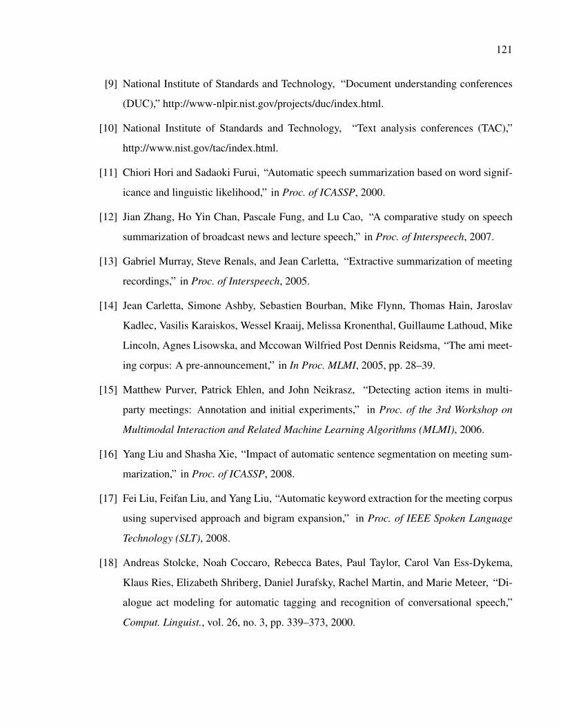
121
[9] National Institute of Standards and Technology, “Document understanding conferences
(DUC),” http://www-nlpir.nist.gov/projects/duc/index.html.
[10] National Institute of Standards and Technology, “Text analysis conferences (TAC),”
http://www.nist.gov/tac/index.html.
[11] Chiori Hori and Sadaoki Furui, “Automatic speech summarization based on word signif-
icance and linguistic likelihood,” in Proc. of ICASSP, 2000.
[12] Jian Zhang, Ho Yin Chan, Pascale Fung, and Lu Cao, “A comparative study on speech
summarization of broadcast news and lecture speech,” in Proc. of Interspeech, 2007.
[13] Gabriel Murray, Steve Renals, and Jean Carletta, “Extractive summarization of meeting
recordings,” in Proc. of Interspeech, 2005.
[14] Jean Carletta, Simone Ashby, Sebastien Bourban, Mike Flynn, Thomas Hain, Jaroslav
Kadlec, Vasilis Karaiskos, Wessel Kraaij, Melissa Kronenthal, Guillaume Lathoud, Mike
Lincoln, Agnes Lisowska, and Mccowan Wilfried Post Dennis Reidsma, “The ami meet-
ing corpus: A pre-announcement,” in In Proc. MLMI, 2005, pp. 28–39.
[15] Matthew Purver, Patrick Ehlen, and John Neikrasz, “Detecting action items in multi-
party meetings: Annotation and initial experiments,” in Proc. of the 3rd Workshop on
Multimodal Interaction and Related Machine Learning Algorithms (MLMI), 2006.
[16] Yang Liu and Shasha Xie, “Impact of automatic sentence segmentation on meeting sum-
marization,” in Proc. of ICASSP, 2008.
[17] Fei Liu, Feifan Liu, and Yang Liu, “Automatic keyword extraction for the meeting corpus
using supervised approach and bigram expansion,” in Proc. of IEEE Spoken Language
Technology (SLT), 2008.
[18] Andreas Stolcke, Noah Coccaro, Rebecca Bates, Paul Taylor, Carol Van Ess-Dykema,
Klaus Ries, Elizabeth Shriberg, Daniel Jurafsky, Rachel Martin, and Marie Meteer, “Di-
alogue act modeling for automatic tagging and recognition of conversational speech,”
Comput. Linguist., vol. 26, no. 3, pp. 339–373, 2000.
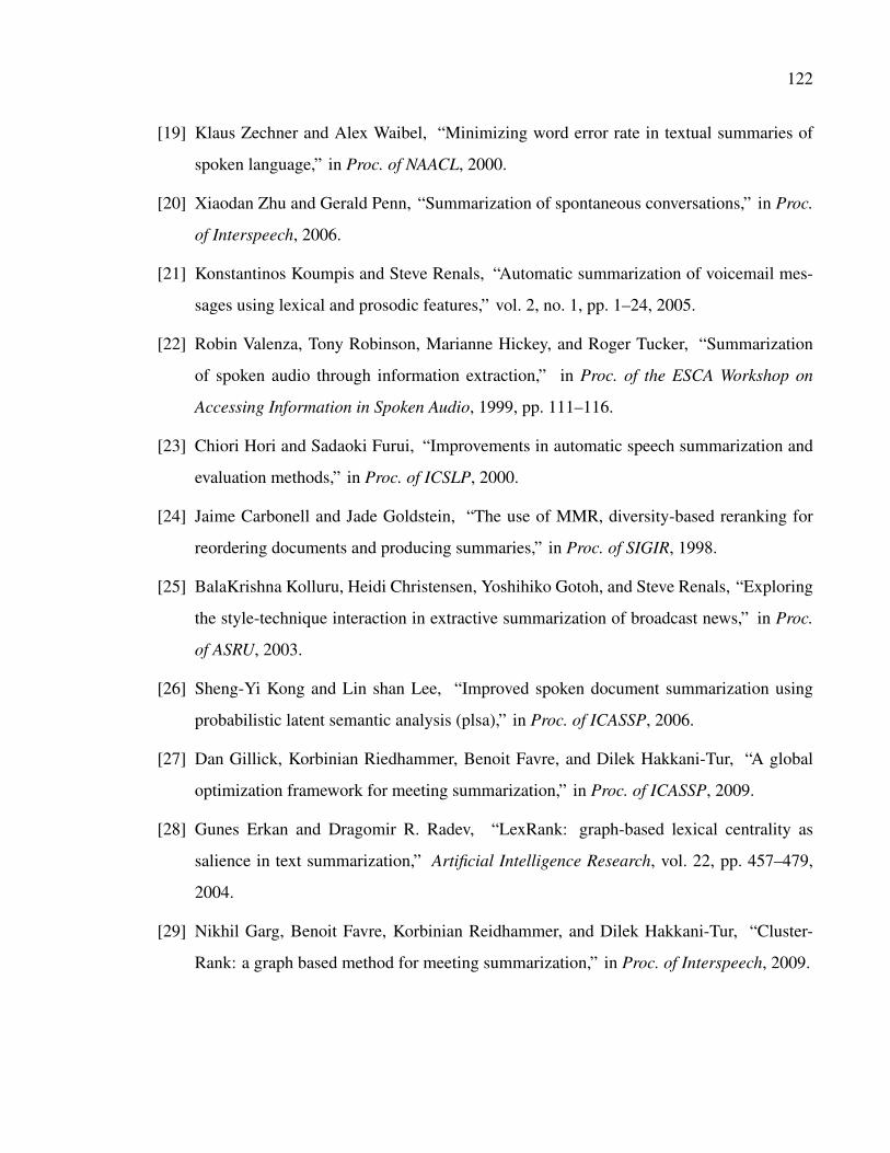
122
[19] Klaus Zechner and Alex Waibel, “Minimizing word error rate in textual summaries of
spoken language,” in Proc. of NAACL, 2000.
[20] Xiaodan Zhu and Gerald Penn, “Summarization of spontaneous conversations,” in Proc.
of Interspeech, 2006.
[21] Konstantinos Koumpis and Steve Renals, “Automatic summarization of voicemail mes-
sages using lexical and prosodic features,” vol. 2, no. 1, pp. 1–24, 2005.
[22] Robin Valenza, Tony Robinson, Marianne Hickey, and Roger Tucker, “Summarization
of spoken audio through information extraction,” in Proc. of the ESCA Workshop on
Accessing Information in Spoken Audio, 1999, pp. 111–116.
[23] Chiori Hori and Sadaoki Furui, “Improvements in automatic speech summarization and
evaluation methods,” in Proc. of ICSLP, 2000.
[24] Jaime Carbonell and Jade Goldstein, “The use of MMR, diversity-based reranking for
reordering documents and producing summaries,” in Proc. of SIGIR, 1998.
[25] BalaKrishna Kolluru, Heidi Christensen, Yoshihiko Gotoh, and Steve Renals, “Exploring
the style-technique interaction in extractive summarization of broadcast news,” in Proc.
of ASRU, 2003.
[26] Sheng-Yi Kong and Lin shan Lee, “Improved spoken document summarization using
probabilistic latent semantic analysis (plsa),” in Proc. of ICASSP, 2006.
[27] Dan Gillick, Korbinian Riedhammer, Benoit Favre, and Dilek Hakkani-Tur, “A global
optimization framework for meeting summarization,” in Proc. of ICASSP, 2009.
[28] Gunes Erkan and Dragomir R. Radev, “LexRank: graph-based lexical centrality as
salience in text summarization,” Artificial Intelligence Research, vol. 22, pp. 457–479,
2004.
[29] Nikhil Garg, Benoit Favre, Korbinian Reidhammer, and Dilek Hakkani-Tur, “Cluster-
Rank: a graph based method for meeting summarization,” in Proc. of Interspeech, 2009.

123
[30] Hui Lin, Jeff Bilmes, and Shasha Xie, “Graph-based submodular selection for extractive
summarization,” in Proc. of ASRU, 2009.
[31] Sameer Raj Maskey and Julia Hirschberg, “Automatic summarization of broadcast news
using structural features,” in Proc. of Eurospeech, 2003.
[32] Anne Hendrik Buist, Wessel Kraaij, and Stephan Raaijmakers, “Automatic summariza-
tion of meeting data: A feasibility study,” in Proc. of CLIN, 2005.
[33] Sameer Maskey and Julia Hirschberg, “Summarizing speech without text using Hidden
Markov Models,” in Proc. of HLT-NAACL, 2006.
[34] Michel Galley, “A skip-chain conditional random field for ranking meeting utterances by
importance,” in Proc. of EMNLP, 2006.
[35] Sameer Maskey and Julia Hirschberg, “Comparing lexical, acoustic/prosodic, structural
and discourse features for speech summarization,” in Proc. of Interspeech, 2005.
[36] Xiaodan Zhu and Gerald Penn, “Comparing the roles of textual, acoustic and spoken-
language features on spontaneous-conversation summarization,” in Proc. of HLT, 2006.
[37] Justin Jian Zhang, Ho Yin Chan, and Pascale Fung, “Improving lecture speech summa-
rization using rhetorical information,” in Proc. of ASRU, 2007.
[38] Gabriel Murray, Steve Renals, Jean Carletta, and Johanna Moore, “Incorporating speaker
and discourse features into speech summarization,” in Proc. of HLT-NAACL, 2006.
[39] Gerald Penn and Xiaodan Zhu, “A critical reassessment of evaluation baselines for speech
summarization,” in Proc. of ACL, 2008.
[40] Shih-Hsiang Lin and Berlin Chen, “A risk minimization framework for extractive speech
summarization,” in Proc. of ACL, 2010.
[41] Klaus Zechner, “Automatic summarization of open-domain multiparty dialogues in di-
verse genres,” Computational Linguistics, vol. 28, pp. 447–485, 2002.
[42] Chiori Hori and Sadaoki Furui, “Advances in automatic speech summarization,” in Proc.
of Eurospeech, 2001.

124
[43] Fei Liu and Yang Liu, “From extractive to abstractive meeting summaries: Can it be done
by sentence compression?,” in Proc. of ACL, 2009.
[44] Gabriel Murray, Giuseppe Carenini, and Raymond Ng, “Interpretation and transformation
for abstracting conversations,” in Proc. of NAACL, 2010.
[45] Chin-Yew Lin, “ROUGE: A package for automatic evaluation of summaries,” in Proc. of
The Workshop on Text Summarization Branches Out, 2004.
[46] Gabriel Murray, Steve Renals, Jean Carletta, and Johanna Moore, “Evaluating automatic
summaries of meeting recordings,” in Proc. of the ACL Workshop on Intrinsic and Ex-
trinsic Evaluation Measures for Machine Translation, 2005.
[47] Feifan Liu and Yang Liu, “Correlation between rouge and human evaluation of extractive
meeting summaries,” in Proc. of ACL-HLT, 2008.
[48] Ani Nenkova and Rebecca Passonneau, “Evaluating content selection in summarization:
The pyramid method,” in Proc. of HLT-NAACL, 2004.
[49] Adam Janin, Don Baron, Jane Edwards, Dan Ellis, David Gelbart, Nelson Morgan, Bar-
bara Peskin, Thilo Pfau, Elizabeth Shriberg, Andreas Stolcke, and Chuck Wooters, “The
ICSI meeting corpus,” in Proc. of ICASSP, 2003.
[50] Elizabeth Shriberg, Raj Dhillon, Sonali Bhagat, Jeremy Ang, and Hannah Carvey, “The
ICSI meeting recorder dialog act (MRDA) corpus,” in Proc. of SigDial, 2004.
[51] Qifeng Zhu, Andreas Stolcke, Barry Chen, and Nelson Morgan, “Using MLP features in
SRI’s conversational speech recognition system,” in Proc. of Interspeech, 2005.
[52] Lidia Mangu, Eric Brill, and Andreas Stolcke, “Finding consensus in speech recognition:
word error minimization and other applications of confusion networks,” Computer Speech
and Language, vol. 14, pp. 373–400, 2000.
[53] Shasha Xie and Yang Liu, “Using corpus and knowledge-based similarity measure in
maximum marginal relevance for meeting summarization,” in Proc. of ICASSP, 2008.

125
[54] Fei Liu and Yang Liu, “What are meeting summaries? an analysis of human extractive
summaries,” in Proc. of SigDial, 2008.
[55] Dragomir Radev, Hongyan Jing, and Malgorzata Budzikowska, “Centroid-based sum-
marization of multiple documents: sentence extraction, utility-based evaluation, and user
studies,” in NAACL-ANLP 2000 Workshop on Automatic summarization, April 2000.
[56] Gabriel Murray and Steve Renals, “Term-weighting for summarization of multi-party
spoken dialogues,” in Proc. of MLMI, 2007.
[57] Rada Mihalcea, Courtney Corley, and Carlo Strapparava, “Corpus-based and knowledge-
based measures of text semantic similarity.,” in Proc. of the American Association for
Artificial Intelligence, September 2006.
[58] Peter Turney, “Mining the web for synonyms: PMI–IR versus LSA on TOEFL,” in Proc.
of the 12th European Conference on Machine Learning, 2001.
[59] Thorsten Brants, “TnT – a statistical part-of-speech tagger,” in Proc. of the 6th Applied
NLP Conference, April 2000.
[60] Ryan McDonald, “A study of global inference algorithms in multi-document summariza-
tion,” in Proc. of 9th ICSLP, 2006.
[61] C.C Chang and C.J Lin, “LIBSVM: a library for support vector machines,” 2001, Soft-
ware available at http://www.csie.ntu.edu.tw/˜cjlin/libsvm.
[62] Julian Kupiec, Jan Pedersen, and Francine Chen, “A trainable document summarizer,” in
Proc. of SIGIR, 1995.
[63] Heidi Christensen, BalaKrishna Kolluru, Yoshihiko Gotoh, and Steve Renals, “From text
summarization to style-specific summarization for broadcast news,” in Proc. of ECIR,
2004.
[64] Marcus A. Maloof, “Learning when data sets are imbalanced and when costs are unequal
and unknown,” in ICML-2003 Workshop on Learning from Imbalanced Data Sets, 2003.

126
[65] Foster Provost, “Machine learning from imbalanced data sets 101,” in Proc. of AAAI
Workshop on Imbalanced Data Sets, 2000.
[66] Benjamin Wang and Nathalie Japkowicz, “Boosting support vector machines for imbal-
anced data sets,” in Journal of Foundations of Intelligent Systems, 2008, vol. 4994, pp.
38–47.
[67] Yang Liu, Nitesh Chawla, Mary Harper, Elizabeth Shriberg, and Andreas Stolcke, “A
study in machine learning from imbalanced data for sentence boundary detection in
speech,” in Computer Speech and Language, 2006, vol. 20, pp. 468–494.
[68] Douglas C. Montgomery, Elizabeth A. Peck, and G. Geoffrey Vining, “Introduction to
linear regression analysis,” July 2006, Wiley-Interscience.
[69] Chao-Ying Joanne Peng, Kuk Lida Lee, and Gary M. Ingersoll, “An introduction to logis-
tic regression analysis and reporting,” in Journal of Education Research, 2002, vol. 96,
pp. 3–14.
[70] Alex J. Smola and Bernhard Sch Olkopf, “A tutorial on support vector regression,” Tech.
Rep., Statistics and Computing, 1998.
[71] George H. John, Ron kohavi, and Karl Pfleger, “Irrelevant features and the subset selec-
tion problem,” in Machine Learning: Proc. of the 11th International Conference, 1994.
[72] Jian Zhang and Pascale Fung, “Speech summarization without lexical features for man-
darin broadcast news,” in Proc. of HLT-NAACL, 2007.
[73] Paul Boersma and David Weenink, “Praat: doing phonetics by computer,”
http://www.praat.org/, 2006.
[74] Shasha Xie and Yang Liu, “Improving supervised learning for meeting summarization
using sampling and regression,” in Computer Speech and Language, 2010, vol. 24, pp.
495–514.
[75] Zheng-Yu Niu, Dong-Hong Ji, and Chew-Lim Tan, “Word sense disambiguation using
labeled propagation based semi-supervised learning,” in Proc. of ACL, 2005.

127
[76] Nguyen Thanh Tri, Nguyen Minh Le, and Akira Shimazu, “Using semi-supervised learn-
ing for question classification,” in Proc. of ICCPOL, 2006.
[77] Rong Liu, Jianzhong Zhou, and Ming Liu, “A graph-based semi-supervised learning
algorithm for web page classification,” in Proc. of sixth International conference on
Intelligent Systems Design and application, 2006.
[78] Je Hun Jeon and Yang Liu, “Semi-supervised learning for automatic prosodic event de-
tection using co-training algorithm,” in Proc. of ACL-IJCNLP, 2009.
[79] Avrim Blum and Tom Mitchell, “Combining labeled and unlabeled data with co-training,”
in Proc. of the Workshop on Computational Learning Theory, 1998.
[80] Andreas Stolcke, Yochai Konig, and Mitchel Weintraub, “Explicit word error minimiza-
tion in N-best list rescoring,” in Proc. of Eurospeech, 1997.
[81] V.H. Quan, M. Federico, and M. Cettolo, “Integrated n-best re-ranking for spoken lan-
guage translation,” in Proc. of EuroSpeech, 2005.
[82] Nicola Bertoldi and Marcello Federico, “A new decoder for spoken language translation
based on confusion networks,” in Proc. of ASRU, 2005.
[83] Ciprian Chelba, Jorge Silva, and Alex Acero, “Soft indexing of speech content for search
in spoken documents,” in Computer Speech and Language, 2007, vol. 21, pp. 458–478.
[84] Tee Kiah Chia, Khe Chai Sim, Haizhou Li, and Hwee Tou Ng, “A lattice-based approach
to query-by-example spoken document retrieval,” in Proc. of SIGIR, 2008.
[85] Lufeng Zhai, Pascale Fung, Richard Schwartz, Marine Carpuat, and Dekai Wu, “Using
n-best lists for named entity recognition from chinese speech,” in Proc. of NAACL, 2004.
[86] Dilek Hakkani-Tur, Frederic Behet, Giuseppe Riccardi, and Gokhan Tur, “Beyond ASR
1-best: using word confusion networks in spoken language understanding,” Computer
Speech and Language, vol. 20, no. 4, pp. 495 – 514, 2006.
[87] Hermann Ney, “Speech translation: Coupling of recognition and translation,” in Proc. of
ICASSP, 1999.

128
[88] Chiori Hori and Sadaoki Furui, “A new approach to automatic speech summarization,”
IEEE Transactions on Multimedia, vol. 5, no. 3, pp. 368–378, 2003.
[89] Shih-Hsiang Lin and Berlin Chen, “Improved speech summarization with multiple-
hypothesis representations and Kullback-Leibler divergence measures,” in Proc. of In-
terspeech, 2009.
[90] Shasha Xie and Yang Liu, “Using confusion networks for speech summarization,” in
Proc. of NAACL-HLT, 2010.

VITA
I received my B.S. degree in electronic and information engineering from Tianjin University, Tian-
jin, China, in 2003, and the M.S. degree in electrical engineering from Tsinghua University, Bei-
jing, China, in 2006. From August 2006, I have been pursuing the Ph.D. degree majoring in
computer science at the University of Texas at Dallas.
My research interests include spoken language processing and understanding, extractive text/speech
summarization, and information retrieval and extraction.
Publications:
[1] Shasha Xie and Yang Liu, “Using N-best Lists and Confusion Networks for Meeting Summa-
rization”, IEEE Transactions on Audio, Speech and Language Processing, to appear.
[2] Shasha Xie and Yang Liu, “Improving Supervised Learning for Meeting Summarization Using
Sampling and Regression”, Computer Speech and Language, V24, pages 495-514, 2010.
[3] Shasha Xie, Hui Lin, and Yang Liu, “Semi-Supervised Extractive Meeting Summarizaqtion
via Co-Training Algorithm”, in Proc. of the International Speech Communication Association
(Interspeech), Makuhari, Japan, September 2010.
[4] Shasha Xie, and Yang Liu, “Using Confusion Networks for Speech Summarization”, in Proc.
of NAACL-HLT, Log Angeles, June 2010.
[5] Yang Liu, Shasha Xie, and Fei Liu, “Using N-best Recognition Output for Extractive Summa-
rization and Keyword Extraction in Meeting Speech”, in Proc. of IEEE International Conference

on Acoustics, Speech and Signal Processing (ICASSP), Dallas, March 2010.
[6] Shasha Xie, Dilek Hakkani-Tur, Benoit Favre, and Yang Liu, “Integrating Prosodic Features in
Extractive Meeting Summarization”, in Proc. of IEEE Automatic Speech Recognition and Under-
standing (ASRU), Merano, Italy, December 2009.
[7] Hui Lin, Jeff Bilmes and Shasha Xie, “Graph-based Submodular Selection for Extractive Sum-
marization”, in Proc. of IEEE Automatic Speech Recognition and Understanding (ASRU), Mer-
ano, Italy, December 2009.
[8] Shasha Xie, Benoit Favre, Dilek Hakkani-Tur, and Yang Liu, “Leveraging Sentence Weights in
a Concept-based Optimization Framework for Extractive Meeting Summarization”, in Proc. of the
International Speech Communication Association (Interspeech), Brighton U.K., September 2009.
[9] Shasha Xie, Yang Liu, Hui Lin, “Evaluating the Effectiveness of Features and Sampling in
Extractive Meeting Summarization”, in Proc. of IEEE Workshop on Spoken Language Technology
(SLT), Goa India, Decemeber 2008.
[10] Shasha Xie and Yang Liu, “Using Corpus and Knowledge-based Similarity Measure in Maxi-
mum Marginal Relevance for Meeting Summarization”, in Proc. of IEEE International Conference
on Acoustics, Speech and Signal Processing(ICASSP), Las Vegas, March 2008.
[11] Yang Liu and Shasha Xie, “Impact of Automatic Sentence Segmentation on Meeting Summa-
rization”, in Proc. of IEEE International Conference on Acoustics, Speech and Signal Processing
(ICASSP), Las Vegas, March 2008.
[12] Yang Liu, Feifan Liu, Bin Liu, and Shasha Xie, “Do Disfluencies Affect Meeting Summariza-
tion: A Pilot Study on the Impact of Disfluencies”, MLMI, 2007.