automatic inferential bias adjustment: optimisation of an

Murdoch University

School of Engineering and Information Technology

Automatic inferential bias adjustment:

Optimisation of an industrial application.

Contains Alcoa Confidential Information.

A report submitted to the School of Engineering and Information Technology, Murdoch University in partial fulfilment of the requirements for the degree of

Bachelor of Engineering Honours

in the disciplines of

Instrumentation and Control Engineering/Industrial Computer Systems Engineering

Prepared by

Craig Maloney

2017

Declaration

I declare that this thesis has been conducted solely by myself and that it has not been

submitted, in whole or in part, in any prior application for a degree at any tertiary education

institution. Except where stated otherwise by reference or acknowledgement, the work

presented is entirely my own.

Signed: _______________________

Name: Craig Warren Maloney

Date: _______________________

Word count of all parts of this report excluding references and appendices: 12, 471

P a g e iii

Abstract

Not all process variables can be directly measured, some require alternative measured

variables together with their known relationship to enable a calculation of an inferred value

of the required variable. As these inferred values rely on a fixed calculation a common

practice in maintaining their accuracy is by continued automatic bias adjustment as a result

of errors determined through laboratory analysis. The focus of the project was to determine

the optimal method of bias adjustment of an industrial application of this process within an

alumina refinery. Specifically, the critical digestion control variable the Blow Off Ratio

(BOR).

The current method of using a cumulative summation (CUSUM) of the errors resulting

from the laboratory analysis with a fixed trigger limit to initiate a bias correction was used

as a reference enabling average error reductions to be determined by the simulated

alternative methods. The standard CUSUM using a multiple of the process standard

deviation to establish a dynamic trigger resulted in average error improvements across all

five digestion units of the initial testing. Optimising both CUSUM trigger parameters (fixed

and dynamic) resulted in minimal average error solution operating outside the definition of

a CUSUM.

Simulation of a standard error filter 𝒃𝒊𝒂𝒔𝒊 = 𝒃𝒊𝒂𝒔𝒊−𝟏 + 𝑲. 𝒆𝒓𝒓𝒐𝒓𝒊−𝟏 as the bias adjustment

method, even though not recommended, provided substantial improvements of 19.9% to

29.4% average error reduction across the tested units. The main cause of this significant

result was found to be a dramatic cyclic drift of the inferred BOR. This resulted in the

poor performance of the CUSUM as its intent is to detect small shifts.

P a g e iv

Additional alternative bias adjustments simulated to maintain the improvements of the

error filter and sustain the performance of the CUSUM during low levels of drift were the

Fast Initial Response (FIR) CUSUM and the Shewhart/CUSUM combination. Of these two

methods, the FIR CUSUM showed no improvement but while the Shewhart delivered

isolated improvement, the optimal error filter delivered consistently better results across

all units tested and differing yearly historical data.

P a g e v

Table of Contents Declaration ........................................................................................................................... ii

Abstract ............................................................................................................................... iii

List of Figures ..................................................................................................................... vii

List of Tables ....................................................................................................................... ix

List of Equations ................................................................................................................. xi

Acknowledgments .............................................................................................................. xii

Acronyms .......................................................................................................................... xiii

Chapter 1: Introduction ................................................................................................... 1

1.1 Literature Review ................................................................................................. 2

1.1.1 Background ................................................................................................... 2

1.1.2 Steady State Identifier Research .................................................................. 4

1.1.3 Inferential Bias Correction Research ............................................................ 6

1.1.4 Aims and Objectives ..................................................................................... 9

Chapter 2: Methods and Simulation Design ................................................................. 11

2.1 Data Collection ................................................................................................... 11

2.2 Simulation ........................................................................................................... 13

2.2.1 Common Code ............................................................................................ 13

2.2.2 Steady State Identifier................................................................................. 15

2.2.3 Current Method ........................................................................................... 16

2.2.4 Standard CUSUM ....................................................................................... 22

2.2.5 CUSUM Optimisation .................................................................................. 24

Chapter 3: Initial Results ............................................................................................... 26

3.1 Steady State Identifier ........................................................................................ 26

3.2 CUSUM Comparison Analysis ........................................................................... 29

Chapter 4: Standard Filter Simulation .......................................................................... 33

P a g e vi

Chapter 5: Standard Filter Results ............................................................................... 34

Chapter 6: Alternative Statistical Filter Simulation ....................................................... 39

6.1 Fast Initial Response CUSUM ........................................................................... 39

6.2 Shewhart and CUSUM Combination ................................................................. 40

Chapter 7: Final Results ............................................................................................... 41

Chapter 8: Discussion ................................................................................................... 47

Chapter 9: Conclusion .................................................................................................. 50

Chapter 10: References .............................................................................................. 51

Appendix ........................................................................................................................... 53

A.1 Reference Documentation Links ............................................................................. 53

A.2 Simulation Code ...................................................................................................... 54

A2.1 Steady State Identification Simulation code ...................................................... 54

A2.2 Current CUSUM Simulation code ...................................................................... 58

A2.3 Standard CUSUM Simulation code ................................................................... 62

A2.4 Standard Error Filter Simulation code ............................................................... 66

A2.5 FIR CUSUM Simulation code ............................................................................ 70

A2.6 Shewhart/CUSUM Simulation code .................................................................. 74

P a g e vii

List of Figures

Figure 2: Data importation from excel MATLAB code. ..................................................... 14

Figure 3: Data simulation range selection MATLAB code. .............................................. 15

Figure 4: R-statistic calculation MATLAB code. ............................................................... 16

Figure 5: Current CUSUM simulation summation and bias adjustment MATLAB code. 18

Figure 6: Test for laboratory MATLAB code. .................................................................... 19

Figure 7: Sample time and time stamp string comparison. .............................................. 20

Figure 8: Simulation inner while loop error calculations................................................... 21

Figure 9: CUSUM simulation reset MATLAB code. ......................................................... 22

Figure 10: Simulation performance indicator calculation and display MATLAB code. .... 22

Figure 11: Standard CUSUM calculation MATLAB code. ................................................ 23

Figure 12: Optimal CUSUM fixed trigger MATLAB code. ................................................ 24

Figure 13: Optimal CUSUM dynamic trigger MATLAB code. .......................................... 25

Figure 14: SSI comparison 11/02/2014 7:30 pm (Location 1, unit 1). ............................. 28

Figure 15: SSI comparison 21/02/2014 1:05am (Location 1, unit 1). .............................. 28

Figure 16: SSI comparison 01/09/2017 12:13 am (Location 1, unit 3). ........................... 29

Figure 17: Current CUSUM plot (Location 1, Unit 1). ...................................................... 30

Figure 18: Standard dynamic trigger CUSUM plot (Location 1, Unit 1). .......................... 30

Figure 19: Optimal dynamic trigger CUSUM plot (Location 1, Unit 1). ............................ 31

Figure 20: Current CUSUM and optimal error filter bias plot (Location 1, unit 1, days 50 to

150 of 2017). ..................................................................................................................... 35


70 of 2017). ....................................................................................................................... 36


60 of 2017). ....................................................................................................................... 37


70 of 2017). ....................................................................................................................... 38

Figure 24: Shewhart/CUSUM control calculations MATLAB code. ................................. 40

Figure 25: Alternative bias adjustment plot (Location 1, unit 1, days 50 to 60 of 2017). 42



Figure 28: All three locations bias comparison (2017). .................................................... 46

P a g e viii

P a g e ix

List of Tables

Table 1: Extracted data yearly ranges. ............................................................................. 13

Table 2: Current CUSUM limiting parameters for each digestion unit. ............................ 17

Table 3: "TimeStamp" and "SampleTime" Excel format example. .................................. 19

Table 4 Sample time and laboratory result data alignment example............................... 21

Table 5: Tuned R-statistic parameter results Location 1 unit 1 (07/08/1017-04/09/2017).

........................................................................................................................................... 26

Table 6: SSI comparison results during 2014 to 2017 (Location 1, unit 1)...................... 27

Table 7: Current and Standard CUSUM bias adjustment average error results (Location

1, 2017). ............................................................................................................................ 30

Table 8: CUSUM Optimal parameter average error results (Location 1, 2017). ............. 31

Table 9: CUSUM simulation percentage of average error reduction. .............................. 32

Table 10: Standard error filter simulation average error results (Location 1, 2017). ....... 34

Table 11: Standard error filter, percentage average error reduction results (Location 1,

2017). ................................................................................................................................ 35

Table 12: Current CUSUM and optimal error filter bias comparison (Location 1, unit 1,

days 50 to 150 of 2017). ................................................................................................... 36


days 50 to 70 of 2017). ..................................................................................................... 37


days 50 to 60 of 2017). ..................................................................................................... 38


days 60 to 70 of 2017). ..................................................................................................... 38

Table 16: FIR CUSUM simulation average error results (Location 1, 2017). .................. 41

Table 17: Alternative bias adjustment results (Location 1, unit 1, days 50 to 60 of 2017).

........................................................................................................................................... 42


........................................................................................................................................... 43


........................................................................................................................................... 44

Table 20: Complete average error reduction results for all simulations (Location 1, 2017).

........................................................................................................................................... 45

P a g e x

Table 21: Location 2 simulation results 2017. .................................................................. 45

Table 22: Location 3 simulation results 2017. .................................................................. 45

Table 23: Optimal error filter average error reduction results (all locations). .................. 46

P a g e xi

List of Equations

1-1 Digestion reaction ...................................................................................................... 2

1-2 R-statistic firstorder filter ............................................................................................ 6

1-3 R-statistic variance 1 ................................................................................................. 6

1-4 R-statistic noise variance 1 ....................................................................................... 6

1-5 R-statistic variance 2 ................................................................................................. 6

1-6 R-statistic noise variance 2 ....................................................................................... 6

1-7 R-statistic ratio ........................................................................................................... 6

1-8 Traditional bias adjustment ....................................................................................... 7

1-9 Standard error filter .................................................................................................... 7

1-10 Standard positive CUSUM ........................................................................................ 8

1-11 Standard negitive CUSUM ........................................................................................ 8

1-12 Standard CUSUM upper control limit ........................................................................ 8

1-13 Standard CUSUM lower control limit......................................................................... 8

1-14 ARL0 Siemund’s approximation ................................................................................. 8

1-15 ARL1 Siemund’s approximation ................................................................................. 8

1-16 CUSUM slope bias correction (standard form) ......................................................... 9

1-17 CUSUM slope bias correction (n=4) ......................................................................... 9

2-1 Current positive CUSUM code equation ................................................................... 18

2-2 Current negitive CUSUM code equation ................................................................... 18

2-3 Standard positive CUSUM code equation ................................................................ 23

2-4 Standard negitive CUSUM code equation ................................................................ 23

2-5 Standard CUSUM trigger code equation .................................................................. 23

P a g e xii

Acknowledgments

Firstly, I would like to acknowledge both my academic and industrial supervisors during

this project, Professor Parisa Arabzadeh Bahri and Mr Pieter Nel. Thank you, both for your

guidance and motivation. Secondly, I thank Benjamin Mossop, Richard Yeates and

Srikanth Jayakumar for taking the time to explain and show the process and equipment

currently used. Also, thank you to Jan Hurst and Nikki Martindale for their professional

insights. Finally, thank you to my wife Cathrine and three sons James, Conor and Blair for

their continued support and understanding throughout the past four years.

P a g e xiii

Acronyms

Al/TC Alumina to total caustic ratio

ARL CUSUM Average Run Length

ARL0 In control average run length

ARL1 Out of control average run length

BOR Blow off ratio

CL Control Language

CUSUM Cumulative sum

FIR Fast Initial Response

LCL Lower control limit

PHD Process Historical Database

SPC Statistical process control

SS Steady state

SSI Steady state identifier

Type I errors False error

Type II errors Undetected error

TS Transient state

UCL Upper control limit

P a g e 1

Chapter 1: Introduction

Measurement of process variables is required to enable control of any process within its designed

parameters. The instrumentation used to measure these process variables provide only an estimation

of the actual process value. These estimations are required to have a certain accuracy depending

on the intent of their use within the control philosophy. Estimation accuracy is affected by many

aspects including the type and quality of instrumentation as well as the physical installation of the

instrument and associated equipment. Many of these inaccuracies result in permanent gross errors

in the estimation which can be corrected via the control system through bias correction. These

estimates also drift from the real value over time due to physical changes occurring to the

instrumentation. These inaccuracies are reduced during periodic maintenance via calibration,

cleaning or replacement of the instrument. These maintenance schedules are predominantly fixed

and usually require the instrument to be taken offline. Consequently, this method of accuracy

improvement by itself cannot ensure the constant accurate online estimation required for many critical

process variables. If the accuracy of critical variables is allowed to drift too far between calibrations

the effect can dramatically impact the profitability of the process and or result in unsafe process

conditions. A conventional method used within the industry to ensure the required level of accuracy

of critical variables is to compare the online measurement with high accuracy measurements

obtained through periodic samples tested within a laboratory. This method enables soft calibration to

be performed at a higher frequency within the control system without taking the instrument offline.

The focus of this Thesis is an industrial application of this method within the alumina refining Bayer

process. The use of data obtained from 12 operational digestion units across three locations provides

the bases for determining a usable solution.

P a g e 2

1.1 Literature Review

This literature review has been compiled to provide the reader with context into the project

background and to introduce the basis of methods used in this paper. It is intended to provide an

understanding into the necessity to conduct this project and the theoretical content of this paper.

1.1.1 Background

1.1.1.1 Bayer Process

In 1888 the patent “A Process for the Production of Aluminum Hydroxide” was issued to Kar Josef

Bayer an Austrian chemist residing in Russia [1]. Now known as the Bayer Process its methods

produce crystalline aluminium hydroxide precipitated from an alkaline solution. This crystalline form

is less complicated to clean compared to the gelatinous form produced from acidic solutions

previously used. This advancement resulted in its widespread commercial adoption following the

commissioning of the first plant in 1893 [2]. The Bayer process comprises three main stages,

extraction, precipitation and calcination. The first stage of the process extraction includes grinding of

the raw bauxite ore. Typical bauxites mined for alumina processing include alumina trihydrate,

boehmite and diaspore predominate. Bauxite ore mined in the darling ranges of Western Australian

contains alumina trihydrate commonly referred to as Gibbsite [3], compounds contained within this

ore are iron oxide, quarts clay minerals and titanium oxide. Separation of the Gibbsite from these

compounds is established by dissolving the bauxite in a hot caustic soda solution. Termed digestion

the resulting reaction (Equation 1-1) produces sodium aluminate and water. This sodium aluminate

slurry referred to as Blow off liquor is then passed through a series of filtration and separation units

to remove the solid compounds as waste.

𝐴𝑙2𝑂3 3𝐻2𝑂 + 2𝑁𝑎𝑂𝐻 → 2𝑁𝑎𝐴𝑙𝑂2 + 4𝐻2𝑂 [1] Equation 1-1

P a g e 3

With the solids removed the sodium aluminate solution, termed green liquor, is passed to the

precipitation stage of the process. Precipitation is the crystallisation of the alumina from the green

liquor as it cools. This cooling occurs as the green liquor is passed through a series of tanks while

being agitated continuously. Small seed crystals are added to the first tank to initiate this precipitation.

As the crystals are formed, they precipitate to the lower of these tanks where they are pumped to the

final stage of the process, calcination. Prior to calcination, the alumina hydrate slurry is washed of

any residual caustic and dried. The remaining hydrate is heated above 1000C during calcination to

cook off the chemically bound hydrogen resulting in the final product of the Bayer process; alumina

[2].

1.1.1.2 Digestion Control

One of the primary variables that determine the alumina yield of the Bayer process is the

alumina/caustic ratio (Al/TC) within the digestion process. Factors affecting the dissolution of gibbsite

in the caustic soda solution are temperature, holding time and caustic soda concentrations [2].

Maximising alumina yield requires the Al/TC ratio exiting digestion after being depressurised, termed

the blow off ratio (BOR), to be controlled as high as possible. If the BOR is set too low, production

targets will not be meet inversely setting of the BOR setpoint too high will not only reduce the

extraction rate due to decreased driving force but also results in the instability of the blow off liquor.

As unstable blow off liquor is passed through the filtration circuit, it cools resulting in auto precipitation.

This formation of alumina hydrate solids before the precipitation tanks not only reduces the final yield

as it is discharged with the process residue but also results in fouling of process equipment.

Bauxite and caustic feed to the digester units are varied to maintain the BOR setpoint and ensure

production rates are met. Due to the narrow operating range of the BOR to ensure production rates

are met, and auto precipitation is prevented, the accuracy of the BOR measurement feedback to the

controller is essential.

P a g e 4

1.1.1.3 Blow Off Ratio Measurement

Without online measurement of the BOR, the digester bauxite and caustic feed rates are fixed. Fixing

these process feeds require regular samples to be analysed by the laboratory with the results

determining required changes of these feed rates. This method results in unknown BOR values

between laboratory sampling, resulting in reduced performance due to unpredicted disturbances.

Advancements in BOR control have been enabled by the development of electrodeless meters used

to measure the digester process conductivity, as it has been established that electrical conductivity

is a linear function of the liquor ratio [1]. Installing conductivity meters to side streams taken from the

digestion process results in online feedback to the controller being established. While this provides

the benefits of online control, other process factors affect the conductivity cell resulting in a shift of

the linear function. This shift if not identified results in the BOR control at an incorrect value. Periodic

laboratory analysis results can be compared with the online measurement to identify this shift. Once

identified, manual adjustment of the cell can be performed to rectify the measurement. This

adjustment may require the cell to be taken offline resulting in loss of continuous control or process

downtime. An online soft calibration can be performed by incorporation of this online conductivity

measurement with periodic laboratory results within the control system. Resultantly improving the

accuracy of the online measurement and reducing the frequency of instrument calibrations. The

optimisation a method of soft calibration for an inferred BOR within an industrial Bayer process is the

focus of this paper.

1.1.2 Steady State Identifier Research

Identification of a steady state (SS) is required for many functions within the process control field

including but not limited to fault detection, model identification, sensor analysis and optimisation [4].

Steady-state identification (SSI), in this case, tests the online process for stability at the time a

P a g e 5

laboratory sample is registered ensuring ideal conditions for a comparison of the two values. Many

methods are proposed within literature with varying similarities. The direct approach incorporates

obtaining a linear approximation of the process data over a given data set. Testing the slope of this

approximation can determine a steady state with a value near to zero. This method while intuitive to

understand requires considerable computation and relies on experience to determine an appropriate

data set for the intended process [5]. Additionally, a turning point in the process could result in a type

II error (undetected instability) as the slope will also register close to zero. The method used by Kim

[6] as well as proposed by Jubien and Bihary [7] uses a data set to calculate the standard deviation

at the time of the sample. During SS the standard deviation will be an indication of the inherent noise

of the inferred value, although during a transient state (TS) the standard deviation will increase. This

method will successfully differentiate between SS and TS with correctly set dataset range and limiting

parameters. The limiting parameter is determined via establishing the variance due to noise from

data during a known process steady state. Therefore, a change in this noise-induced process

variance requires the parameter to be altered to maintain SSI performance. A differing method used

by Vasyutynskyy [8] calculates a ratio of two sequential data set means. Resulting in a ratio value

tending to one during SS, as a TS would lead to a difference in the sequential mean values tending

the ratio further from unity. This method also uses the standard deviation of each data set as a scaling

factor alleviating the issue of having to adjust the limiting factor of the current approach due to process

variance changes. However, as with the direct approach, the means prior and post a turning point

could result in identical means again leading to type II errors. An alternative method, the R-statistic,

also rectifying the issue of changes in process variances is presented by Cao and Rhinehart [4]. The

principle operation of this technique calculates the ratio of two variances attained through differing

methods. This first variance 𝒔𝟏,𝒊𝟐 is computed by the difference between the real data and a filtered

value of the real data (Equation 1-2, Equation 1-3 and Equation 1-4) [4]. In practice, this difference

will be minimal during a SS and increase throughout a TS due to the lagging nature of the filtered

value. The second variance 𝒔𝟐,𝒊𝟐 represents the difference between sequential real data values

P a g e 6

(Equation 1-5 and Equation 1-6) [4]. The value obtained from the ratio 𝑹𝒊 in Equation 1-7 of these

two variances will tend toward unity during a SS. Again, due to the inherent lag of the filtered data,

the ratio term will increase during a TS proportional to the transient. Comparison of this ratio with a

determining parameter will indicate when the variable is at SS or TS.

𝒙𝒇,𝒊 = 𝝀𝟏𝒙𝒊 + (𝟏 − 𝝀𝟏)𝒙𝒇,𝒊−𝟏 [4] Equation 1-2

𝒗𝒇,𝒊𝟐 = 𝝀𝟐(𝒙𝒊 − 𝒙𝒇,𝒊−𝟏)

𝟐+ (𝟏 − 𝝀𝟐)𝒗𝒇,𝒊−𝟏

𝟐 [4] Equation 1-3

𝒔𝟏,𝒊𝟐 =

𝟐−𝝀𝟏

𝟐𝒗𝒇,𝒊


𝜹𝒇,𝒊𝟐 = 𝝀𝟑(𝒙𝒊 − 𝒙𝒊−𝟏)𝟐 + (𝟏 − 𝝀𝟑)𝜹𝒇,𝒊−𝟏


𝒔𝟐,𝒊𝟐 =

𝜹𝒇,𝒊𝟐

𝟐 [4]

Equation 1-6

𝑹𝒊 =𝒔𝟏,𝒊

𝟐

𝒔𝟐,𝒊𝟐 =

(𝟐−𝝀𝟏)𝒗𝒇,𝒊𝟐

𝜹𝒇,𝒊𝟐 [4] Equation 1-7

1.1.3 Inferential Bias Correction Research

Comparison of a steady state process value with laboratory analysis results can identify if the process

online inferred value has drifted from the actual value. This detected shift can then be corrected by

adjusting a bias value added to the inferential to reduce the calculated error. The traditional method

of calculating the bias by adding the previous bias with the obtained error (Equation 1-8) would, in

theory, remove 100% of the error. However, in the event of random errors during sampling and

laboratory analysis, additional random errors would be introduced to the inferred value [9]. These

incorrect adjustments would have flow-on effects in the process and depending on their magnitude

could result in production loss and or unsafe conditions. A common practice to reduce the effect of

random errors is the inclusion of an error filter term 𝑲 (Equation 1-9), resulting in only a selectable

portion of the error being used to adjust the bias. Error filtering will only reduce random errors,

therefore, to increase confidence in a required bias adjustment a method to establish the occurrence

of continued drift over a number of sampling periods would be required.

P a g e 7

𝒃𝒊𝒂𝒔𝒊 = 𝒃𝒊𝒂𝒔𝒊−𝟏 + 𝒆𝒓𝒓𝒐𝒓𝒊−𝟏 [10] Equation 1-8

𝒃𝒊𝒂𝒔𝒊 = 𝒃𝒊𝒂𝒔𝒊−𝟏 + 𝑲. 𝒆𝒓𝒓𝒐𝒓𝒊−𝟏 [10] Equation 1-9

A conventional method to monitor a measured process variable in relation to the desired value is

statistical process control (SPC). Control charts, one of the primary tools used in SPC, comprises of

an upper and lower control limit (UCL and LCL respectively). Data exceeding these limits trigger

notification the monitored variable parameter has reached an unacceptable deviation from its desired

value. Different control charts are used to monitor the mean and variance of a measured variable,

due to the issues concerning the inferred error from the real value, SPC control methods for

monitoring the mean are of great interest. Shewhart control charts developed by Walter A. Shewhart

in 1920 [11] are commonly used for online SPC. The �̅� control chart monitors a variable’s mean of a

data set while setting the upper and lower control limits at a multiple of σ (monitored variables

standard deviation), usually 3σ. Due to the periodic sampling period used in the BOR soft calibration,

a variation of this Shewhart control chart designed for individual measurements would be more

appropriate. The concern with this type of control chart is its insensitivity to small shifts in the process

mean [11]. An alternative control chart used to monitor the mean of a process is the cumulative sum

(CUSUM) control chart and is commonly used for laboratory updating of inferential parameters.

CUSUM charts are used to detect small and persistent shifts in a process mean and are

predominantly used with individual observation data [12]. The Tabular CUSUM (Equation 1-10 and

Equation 1-11) includes two sides one accumulating positive 𝑪𝒊+ and the other negative 𝑪𝒊

− deviations

from a reference 𝝁𝟎 (variable setpoint). The parameter 𝑲 (slack value) is often selected to be half the

difference between the reference and the magnitude of shift in the process variable 𝒙𝒊 that is required

to be promptly detected. Other parameters required to be set are the UCL and LCL. A proven value

for these limits is 5 times the process standard deviation 𝝈 (Equation 1-12 and Equation 1-13) and

symbolised by 𝑯 [11].

P a g e 8

𝑪𝒊+ = 𝒎𝒂𝒙[𝟎, 𝒙𝒊 − (𝝁𝟎 + 𝑲) + 𝑪𝒊−𝟏

+ ] [11] Equation 1-10

𝑪𝒊− = 𝒎𝒂𝒙[𝟎, (𝝁𝟎 − 𝑲) − 𝒙𝒊 + 𝑪𝒊−𝟏

− ] [11] Equation 1-11

𝑼𝑪𝑳 = 𝑯 = 𝒉𝝈 [11] Equation 1-12

𝑳𝑪𝑳 = −𝑯 = −𝒉𝝈 [11] Equation 1-13

The values of both parameters affect the time between type I (false alarm) errors during stable

control, referred to as the in control average run length (ARL0) in SPC. A small ARL0 will result in

tighter control and increased type I errors. Inversely higher values of an ARL0 will result in type II

errors. With high sampling frequencies, a higher ARL0 is ideal as frequent false triggers would affect

the process. Increased time between samples would require a lower ARL0 to ensure shifts of the

inferential are corrected within an acceptable time. When designing a CUSUM, an important aspect

is the out of control average run length ARL1. This value is the number of summation reiterations

required to trigger a specific magnitude of shift. In the intended context an ARL1 would be the number

of samples required to trigger a bias adjustment in the event of an inferred shift. Both ARL values

can be calculated with Siegmund’s approximation (Equation 1-14 and Equation 1-15) with

parameters 𝒌, 𝒉 and 𝜹 where 𝒌 =𝑲

𝝈 and 𝜹 is the shift in units of 𝝈. Using these approximations, it is

possible to calculate the required control limits for a CUSUM to trigger with an acceptable 𝐴𝑅𝐿1 for a

given shift.

𝑨𝑹𝑳𝟎 ≈𝒆𝒙𝒑[𝟐𝒌(𝒉+𝟏.𝟏𝟔𝟔)]−𝟐𝒌(𝒉+𝟏.𝟏𝟔𝟔)−𝟏

𝟐𝒌𝟐 [11] Equation 1-14

𝑨𝑹𝑳𝟏 ≈𝒆𝒙𝒑[𝟐(𝜹−𝒌)(𝒉+𝟏.𝟏𝟔𝟔)]−𝟐(𝜹−𝒌)(𝒉+𝟏.𝟏𝟔𝟔)−𝟏

𝟐(𝜹−𝒌)𝟐 [12] Equation 1-15

When the designed CUSUM has identified an unacceptable inferential shift and triggered, an

adjustment is made to the bias to correct the inferential error. The simplest method to determine the

required adjustment uses an average of the errors obtained during the summation leading to the

P a g e 9

trigger. An alternative approach is to use the slope of the CUSUM to determine the magnitude of the

correction required. For this approach the derived bias correction Equation 1-16 requires selection of

the number of previous measurements 𝒏 to determine the CUSUM slope. A combination of the

CUSUM slope and error filter is an additional option in calculating the bias adjustment [10], as an

example when 𝒏 = 𝟒 Equation 1-17 indicates the bias adjustment. Once the bias is adjusted the

CUSUM is reset so both 𝑪𝒊+ and 𝑪𝒊

− are set to zero.

𝒃𝒊𝒂𝒔𝒏+𝟏 = 𝒃𝒊𝒂𝒔𝒏 −𝟔

𝒏(𝒏+𝟏)(𝒏+𝟐)∑ 𝒊(𝒏 − 𝒊 + 𝟏)𝒆𝒓𝒓𝒐𝒓𝒏−𝒊+𝟏

𝒏𝒊=𝟏 [10] Equation 1-16

𝒃𝒊𝒂𝒔𝒏+𝟏 = 𝒃𝒊𝒂𝒔𝒏 − 𝑲 (𝟐𝒆𝒓𝒓𝒐𝒓𝒏+𝟑𝒆𝒓𝒓𝒐𝒓𝒏−𝟏+𝟑𝒆𝒓𝒓𝒐𝒓𝒏−𝟐+𝟐𝒆𝒓𝒓𝒐𝒓𝒏−𝟒

𝟏𝟎) [10] Equation 1-17

1.1.4 Aims and Objectives

The overarching aim of this Thesis is to establish an optimal method of automatic bias adjustment of

the inferred BOR of a number of physical Bayer processess. Two main objectives have been

identified to enable measurable improvement of the current method. Firstly, a robust method of

determining the process is at steady state ensuring reliable comparison between the online and

periodic measurements. The R-statistic alternative to the current standard deviation method of SSI

represented by Equation 1-2 to Equation 1-7 will be tested and analysed. This analysis will provide

a gauge to the suitability of this approach for the intended application. Secondly, optimisation of the

method used in identifying and assessing online measurement shift enabling an accurate bias

adjustment. This second objective will be the key focus of this Thesis. Simulation of the current

method with historical data obtained from a number of refineries and digestion units will be compared

with the identified alternatives and modifications including:

1. Dynamic control limits as a function of standard deviation (Equation 1-12 and Equation 1-13).

2. The standard CUSUM with slack parameter K (Equation 1-10 and Equation 1-11).

3. The traditional filtering method (Equation 1-9).

P a g e 10

Performance of the various methods will be measured by the average error between the inferred

BOR and an accepted laboratory result. Additional measures of the differing CUSUMs will be used

such as the average run length between bias updates providing a performance gauge of their balance

between type I and type II errors.

P a g e 11

Chapter 2: Methods and Simulation Design

Identification of the optimal method of BOR bias adjustment requires data from each method to be

analysed for evaluation. Implementation of each alternative method cannot be initiated online as the

resulting disturbance to the process would be unpredictable and present unacceptable financial risk

to the company. Therefore, simulation of various BOR bias adjustment methods requires an offline

program so that production is not affected. The use of MATLAB as the programming platform for the

simulations was adopted as it provided the necessary functions for each simulation. Additional

software is also necessary to enable the extraction of historical data from the systems Process

Historical Database (PHD) and to enable graphical analysis of the results. A complete list of the

required software is as follows:

• Mathworks, MATLAB, revision r2014a minimum. – The platform used for the simulation

algorithm code.

• Honeywell, DOC4000. – Provides access to the control language code of the control system.

• Honeywell, Uniformance Process Studio. – Enables identification of the complete tags

required for extraction of data from the PHD and initial analysis of raw data.

• Honeywell, Uniformance Excel companion. – Enables Microsoft Excel to extract data from

the PHD.

• Microsoft, Excel. – Data extraction from PHD and MATLAB.

2.1 Data Collection

To determine the consistency of a simulation methods performance results are required from differing

data sets from several digestion units. Data from twelve digestion units across three locations were

obtained. Five units from location 1 and location 2 as well as two units from location 3. Each

P a g e 12

simulation requires historical process data to ensure they are suited to the measured process

dynamics. The historical data sets required for each unit of each location from the PHD is as follows:

• Time stamp – Control system data point time stamp.

• BOR – The bias-corrected inferential of the Blow Off Ratio.

• Bias – Bias magnitude calculated via the current adjustment algorithm.

• Standard deviation – Calculated standard deviation of process variable dataset at time of

laboratory sample.

• BOR Average – Calculated BOR average of process variable dataset at time of laboratory

sample.

• Error – BOR error determined via current control system.

• Laboratory sample – BOR value obtained through laboratory analysis.

• Sample time – Documented time of manual sample for BOR laboratory analysis.

Identification of the correct system tags for each of the historical data sets requires the control

language (CL) code accessed through Honeywell’s DOC4000 portal. The CL code enables the

required package input and output variables to be identified. Once the identifier for each I/O data set

has been obtained through the DOC4000 portal, each complete system tag is obtained via a search

in Uniformance Process Studio. Extraction of the historical data requires Microsoft excel with the

Uniformance Excel Companion add-in, and the established complete tags (links to user and help

guides for the required software are included in Appendix A.1. Excel workbooks created for each

location with worksheets for each unit provide ease of data extraction via MATLAB using the “xlsread”

function. With the use of Uniformance Excel companion import snapshot data to excel from the

Process Historical Database (PHD). Each snapshot data set is to have data points with an interval of

one minute and contain data from a four-week duration (instructions for excel data extraction can be

found in the Uniformance Excel Companion Users Guide in Appendix A.1). The reasoning for

extracting only four weeks of data is due to a maximum number of data points that can be extracted

P a g e 13

by this method. Data from each four-week workbook are manually combined to create workbooks

containing yearly data. The range of each locations yearly data spreadsheet is indicated in Table 1.

Table 1: Extracted data yearly ranges.

Location Year Start date End date

Location 1

2017 23/01/2017 02/10/2017

2016 25/01/2016 23/01/2017

2015 03/01/2015 25/01/2016

2014 04/01/2014 03/01/2015

Location 2

2017 16/01/2017 23/10/2017

2016 18/01/2016 16/01/2017

2015 19/01/2015 18/01/2016

2014 20/01/2014 10/01/2015

Location 3

2017 06/01/2017 13/10/2017

2016 08/01/2016 06/01/2017

2015 09/01/2015 08/01/2016

2014 08/01/2014 09/01/2015

2.2 Simulation

All simulations share common code enabling importation and selection of data required for the tests

being performed. Additionally, each differing test requires custom code designed to enable accurate

simulation of the specific test. Examples and explanation of the code used throughout this project

are provided throughout this section to assist any reproduction of the obtained results. Appendix A.2

contains the complete code of all simulation and analysis programmes.

2.2.1 Common Code

Each simulation requires importation of historical data from the Excel files containing the yearly data

as indicated in Table 1. This is enabled with the use of the MATLAB “xlsread” function requiring the

filename, sheet name and data cell range of the Excel spreadsheet containing the required data. The

example code shown in (Figure 1) imports the required data from location 1, unit 1 for the year of

2017. Note the “filename”, “sheet” and the data cell ranges (“###_xlRange”) require manual entry.

P a g e 14

This manual entry allows a single program to be manipulated to extract data from the required excel

spreadsheet. Due to the custom data type of the time-stamp and laboratory-time extracted from the

PHD, these date and time strings are required to be extracted from the cell data as shown on lines

18 and 19 of Figure 1.

Figure 1: Data importation from excel MATLAB code.

Additional common code allowing only a selected range of the imported data to be analysed by the

method being tested is shown in (Figure 2). This additional code allows sections of data obtained

during unit shut down to be disregarded from the simulation test. Subarrays are created by adjusting

the “subtime” and “subsize” variables for the required data range. The “subtime” variable selects the

midpoint of the required data set, and the “subsize” variable identifies the range of data either side of

the midpoint. For example, by commenting out lines 26 and 27 with “%” then uncommenting out lines

28 and 29 by removing the “%” from each line of the code in Figure 2, each sub-array will have a

range of 144000 data points from index 72000 to 216000 of the original imported data array.

P a g e 15

Figure 2: Data simulation range selection MATLAB code.

2.2.2 Steady State Identifier

Simulation of the current SSI being a limiting factor of the inferential data set standard deviation was

simply achieved with the MATLAB “std’ function. The R-statistic simulation requires Equation 1-2 to

Equation 1-7 to be implemented in the simulation code enabling the ratio of the two variances to be

calculated. The recommended filtering term values of 𝝀𝟏 = 𝟎. 𝟐, 𝝀𝟐 = 𝟎. 𝟏 and 𝝀𝟑 = 𝟎. 𝟏 [4] were used

in the simulations to provide a balance of type I and type II errors. The code for the R-statistic

caculations is displayed in Figure 3 where “subRawData” is the BOR value obtained from the PHD.

During the simulation some indicators are established to assist in the analysis of the SSI methods

and are listed as follows:

• Laboratory sample count – this is the total number of laboratory sample results entered into

the PHD for the time period tested.

• Current SSI acceptance count – this is the number of the tests the current SSI resulted in a

SS (total number of tests is equal to the laboratory sample count).

• R-statistic acceptance count - this is the number of the tests the R-statistic SSI resulted in a

SS (total number of tests is equal to the laboratory sample count).

P a g e 16

Figure 3: R-statistic calculation MATLAB code.

2.2.3 Current Method

Simulation of the current CUSUM method enables a reference to compare results of differing

CUSUM’s and alternative methods. Simulation within the same platform (MATLAB) ensures the

results are not affected by factors such as manual bias changes that are performed for various

reasons. Parameters required to simulate the current BOR bias correction method are as follows:

• trig_val – the constant trigger value of the CUSUM initiating a bias adjustment.

• sd_lo – the minimum standard deviation of the BOR dataset (current process SSI low limit).

• sd_hi – the maximum standard deviation of the BOR dataset (current process SSI high limit).

• lab_lo – the minimum laboratory analysis result (laboratory analysis random error outlier

identifier low limit).

• lab_hi – the maximum laboratory analysis result (laboratory analysis random error outlier

identifier high limit).

• max_err – the maximum error that is used for calculations (additional random error outlier

limiter).

• max_adj – the maximum bias adjustment value (minimises the effect of any random errors

not identified).

• x_val – the BOR data set range determinator (i.e. x_val=10 results in a data set range of 20

minutes, 10 minutes either side of the sample time).

P a g e 17

The parameter values obtained for each unit via the DOC4000 portal of each location are contained

in Table 2. In addition to the current CUSUM simulation, these values are to be used in all other

simulations to ensure consistency with exception to the “trig_val” which is altered in the process of

optimisation.

Table 2: Current CUSUM limiting parameters for each digestion unit.

Parameter Location 1 Location 2 Location 3

Unit 1 Unit 2 Unit 3 Unit 4 Unit 5 All Units All Units

trig_val 0.014 0.012 0.014 0.01 0.01 0.014 0.017

sd_hi 0.005 0.005 0.005 0.005 0.005 0.002 0.01

sd_lo 0 0 0 0 0 0 0

lab_hi 0.8 0.8 0.8 0.8 0.8 0.8 0.8

lab_lo 0.65 0.65 0.65 0.65 0.65 0.4 0.4

max_err 0.015 0.015 0.015 0.015 0.015 0.015 0.018

max_adj 0.005 0.005 0.005 0.005 0.005 0.005 0.005

x_val 10 10 10 10 10 10 10

As the current CUSUM within the control system determines the bias term of the BOR inferential an

array (“subRawData”) of the raw inferred BOR historical data is obtained by subtracting the bias data

array “subBiasData” from the BOR data array “subBORData”. The simulated bias corrected BOR

“SimBOR” is then established by adding the calculated bias obtained from the simulation “SimBias”

to this raw BOR. This simulated BOR together with the imported laboratory analysis results enables

an error value (“SimErr”) to be calculated. This method assumes 100% accuracy of the laboratory

results when in practice gross and random errors occur. This assumption is made as the parameters

contained in Table 2 have been established to remove the significant outliers from the CUSUM

calculations.

A form of CUSUM without the slack parameter of Equation 1-10 and Equation 1-11 is the statistical

filter currently implemented, where 𝛍𝟎 and 𝐱𝐢 are the laboratory result and, determined process mean

value respectively. Resultantly, the positive and negative CUSUM summations as are calculated with

Equation 2-1 and Equation 2-2 respectively. When the limiting parameters are meet an “if” function

permits these calculations within the simulation code as indicated on lines 151 and 152 of Figure 4.

P a g e 18

The permitted errors are summed (“SimErrSum”) and counted (“SimErrCnt”) to enable an average

error of the simulated CUSUM to be derived and used as the primary performance indicator.

𝒑𝒐𝒔_𝒔𝒖𝒎𝒊 = 𝒎𝒂𝒙[0, 𝒑𝒐𝒔_𝒔𝒖𝒎𝒊−𝟏 + (𝝁𝟎 − 𝒙𝒊)] Equation 2-1

𝒏𝒆𝒈_𝒔𝒖𝒎𝒊 = 𝒎𝒊𝒏[𝟎, 𝒏𝒆𝒈_𝒔𝒖𝒎𝒊−𝟏 + (𝝁𝟎 − 𝒙𝒊)] Equation 2-2

Once either of the summation (“pos_sum” or “neg_sum”) values exceed the set trigger limit, a new

bias adjustment calculation is initiated. This new bias adjustment (“Sim_n_adj”) as shown in lines

162 and 166 of Figure 4 is an average of the errors since the last adjustment. Similar to the

determination of the simulation average error a simulation average run length is obtained by

establishing a trigger count (“SimTrigCnt”) and ARL sum (“ARLsum”) during bias adjustments.

Figure 4: Current CUSUM simulation summation and bias adjustment MATLAB code.

A sample of the “TimeStamp” and “SampleTime” data extracted from the PHD within an Excel

spreadsheet can be seen in Table 3. This example shows the time required to analyse and enter the

sample results into the control system was 54 minutes. To enable the laboratory sample results to

be compared with the average of the inferred BOR value at the time the sample was extracted from

the process cascaded while loops are required within the Matlab code. The cascaded loops enabled

the simulation to identify the element of the online array data sets (the i-54 element in the example

P a g e 19

shown in Table 3) that corresponds to the data within the laboratory analysis array data set (the I

element in the example shown in Table 3). This is achieved by the outer loop indexing through the

array elements performing the main calculations for the bias and BOR values. Meanwhile, during this

indexing, the concurrent “SampleTime” array elements are compared as shown on line 108 of Figure

5. The “strcmp” (string comparison) MATLAB function indicates when a new laboratory sample value

has been entered into the control system.

Table 3: "TimeStamp" and "SampleTime" Excel format example.

Index Timestamp Sample time

i-55 23/01/2017 0:17 22/01/2017 19:53

i-54 23/01/2017 0:18 22/01/2017 19:53

i-53 23/01/2017 0:19 22/01/2017 19:53

* * *

* * *

i-1 23/01/2017 1:11 22/01/2017 19:53

i 23/01/2017 1:12 23/01/2017 0:18

i+1 23/01/2017 1:13 23/01/2017 0:18

Figure 5: Test for laboratory MATLAB code.

Due to the PHD data importation into Excel, all the time stamp data strings have zero seconds within

the time section. However, the sample times are recorded to the nearest second as indicated in

Figure 6. Therefore, to allow direct comparison of these strings once a new sample has been

identified a new “TempTime” string is established with the code indicated on lines 110 to 114 of

P a g e 20

Figure 5. Therefore, allowing determination of the BOR data to the nearest minute. Note: simpler

code can be established if using newer MATLAB revisions as advanced functions have been made

available. This “TempTime” contains the date and time of the current “subSampleTime” element with

the seconds set to zero.

Figure 6: Sample time and time stamp string comparison.

To establish the error of the inferred BOR at the time of the sample extraction an inner while loop

indexes from the beginning of the data strings comparing the “TempTime” and “subTimeStamp”. This

enables the data set of the simulated BOR required to be obtained at the time the laboratory sample

was taken. The process average and standard deviation of the obtained dataset are calculated with

the “mean and “std” MATLAB functions respectively. The error calculation as indicated on line 133 of

Figure 7 uses the laboratory result value two array elements post the current index. This allows for

the inconsistent data importation into the control system at the time of laboratory result entry. An

example of this is illustrated in Table 4 where the new BOR laboratory result “B” is contained an array

element after the new sample time was indicated.

P a g e 21

Figure 7: Simulation inner while loop error calculations.

Table 4 Sample time and laboratory result data alignment example.

Index Sample time Laboratory value

i-2 22/01/2017 19:53 A

i-1 22/01/2017 19:53 A

i 23/01/2017 0:18 A

i+1 23/01/2017 0:18 B

i+2 23/01/2017 0:18 B

After the CUSUM has initiated a bias adjustment all CUSUM parameters are reset as indicated by

the code on lines 171 to 185 of Figure 8. Additionally, adjustments are limited to the set maximum

adjustment to limit the effect of any random errors that were not identified by the previous limiters.

The final calculations of the outer loop are the simulated bias and BOR values. The loop then indexes

and the code is continually executed until the end of the sub arrays. Following this, the average error

of both the simulated and raw BOR are calculated and displayed together with the ARL, trigger count

and lab sample count (Figure 9). These additional values provide the performance indicators required

for simulation comparisons.

P a g e 22

Figure 8: CUSUM simulation reset MATLAB code.

Figure 9: Simulation performance indicator calculation and display MATLAB code.

2.2.4 Standard CUSUM

The currently adopted CUSUM method used for the automatic bias adjustment of the BOR inferential

indicated in Equation 2-1 and Equation 2-2 does not include the slack factor 𝑲 of the standard

CUSUM introduced in Chapter 1.1.3 (Equation 1-10 and Equation 1-11). Additionally, and most

importantly the standard CUSUM incorporates a dynamic trigger value as a multiple of the measured

variables standard deviation (Equation 1-12 and Equation 1-13). Therefore, simulation of the

standard CUSUM enables comparison to the current method to establish any benefits of these

additional parameters.

The core code of the standard CUSUM is the same as the current CUSUM code with the exception

to the CUSUM calculations and the addition of the 𝒌 and 𝒉 parameters as indicated in Equation 2-3

P a g e 23

to Equation 2-5 where 𝝁𝟎 the reference point is the laboratory analysis result, 𝒙𝒊 is the average of the

simulated BOR data set and 𝝈 is the standard deviation of the same data set. The additional

parameter 𝝈𝒂𝒗𝒈 used to calculate the dynamic trigger in Equation 2-5 is an average of the standard

deviation values obtained during the current CUSUM run as indicated by the code on lines 148 to

151 of Figure 10. Resetting of this parameter is performed with other CUSUM parameters on the

initiation of a bias adjustment.

𝒑𝒐𝒔_𝒔𝒖𝒎𝒊 = 𝒎𝒂𝒙[𝟎, (𝝁𝟎 − (𝒌𝝈)) − 𝒙𝒊 + 𝒑𝒐𝒔_𝒔𝒖𝒎𝒊−𝟏] Equation 2-3

𝒏𝒆𝒈_𝒔𝒖𝒎𝒊 = 𝒎𝒊𝒏[𝟎, (𝝁𝟎 − (𝒌𝝈)) − 𝒙𝒊 + 𝒏𝒆𝒈_𝒔𝒖𝒎𝒊−𝟏] Equation 2-4

𝒕𝒓𝒊𝒈_𝒗𝒂𝒍 = 𝒉𝝈𝒂𝒗𝒈 Equation 2-5

Figure 10: Standard CUSUM calculation MATLAB code.

Standard CUSUM simulation tests involve introducing one new parameter at a time to assess their

individual effects on the average error. However, setting parameter 𝒌 to zero Equation 2-3 and

Equation 2-4 are equivalent to Equation 2-1 and Equation 2-2 of the current CUSUM. This removal

of the slack factor allows the impact of the dynamic trigger to be assessed before the slack factor is

introduced. The typical values for these two parameters as indicated in Chapter 1.1.3 of 𝒉 = 𝟓 and

𝒌 = 𝟎. 𝟓 are set in the standard CUSUM simulations.

P a g e 24

2.2.5 CUSUM Optimisation

Analysis of the average errors obtained from the current CUSUM and the standard CUSUM

simulations described in Chapters 2.2.3 and 2.2.4 provide an indication of any error reductions with

a dynamic CUSUM trigger of 𝒉 = 𝟓 in comparison to the fixed triggers of each unit tested. To obtain

results that indicate the most appropriate method in determining the trigger value (fixed or dynamic)

optimal values for each of these parameters are required.

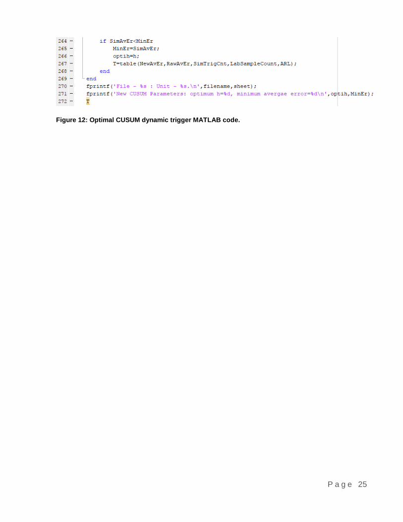
Addition of the “for loop” function within MATLAB to the existing CUSUM simulation programmes

allows the programmes to run a set number of times altering a parameter each cycle. Establishment

of the parameter value resulting in the minimum average error for each case is indicated in the code

within Figure 11 and Figure 12. On completion of the set number of cycles, the optimal parameter

value and the corresponding minimum average error is displayed together with other performance

indicators recorded in the previous simulations.

Due to the currently adopted fixed trigger values found in Table 2 ranging from 0.01 to 0.017, ten

fixed triggers were tested from 0.01 to 0.1 in increments of 0.01 to find the optimum value. Likewise,

using the typical value of 𝒉 = 𝟓 as the middle of the test values to determine the optimal dynamic

trigger another ten values were tested from 1 to 10.

Figure 11: Optimal CUSUM fixed trigger MATLAB code.

P a g e 25

Figure 12: Optimal CUSUM dynamic trigger MATLAB code.

P a g e 26

Chapter 3: Initial Results

To provide a measure of consistency with the results obtained all five of the units at Location 1 were

selected for initial simulations. Therefore, requiring each simulation to run with five differing raw data

sets obtained from the PHD. Comparing the results of a number of alternate data sets minimises the

effect of abnormalities that may exist in the raw data. Results are displayed in tabular form together

with associated data plots to assist initial discussion of each set of results.

3.1 Steady State Identifier

A four-week dataset from 07/08/2017 to 04/09/2017 for unit 1 of Location 1 was used to manually

tune the R-statistic so that the simulation results were similar to the current SSI. The results obtained

with the tuned R limiting parameter set to 5 are displayed in Table 5, clearly indicating similar

performance between the two SSI methods. Simulations with the same tuned R-statistic were

performed for the remaining four units for the same period resulting in slight variation in the differing

methods acceptance.

Table 5: Tuned R-statistic parameter results Location 1 unit 1 (07/08/1017-04/09/2017).

R-statistic SSI results (Location 1 07/08/2017 to 04/09/2017)

Laboratory

sample count

Current SSI acceptance

count

R-statistic SSI acceptance

count


percent


percent

Unit 1 114 85 85 75 75

Unit 2 111 79 73 71 66

Unit 3 121 82 83 68 69

Unit 4 113 60 71 53 63

Unit 5 122 91 193 75 84

Additional simulation for differing PHD datasets of periods during 2014, 2015 and 2016 are presented

in Table 6 indicate the R-statistic results in lower acceptance percentage during the earlier years.

The results obtained with the current SSI, however, provide less acceptance difference. This could

P a g e 27

be an indication that the R-statistic is affected by changes in the inferential variance over time. Since

the main reasoning in implementing this method was to alleviate the need of adjustment due to

inferential variance additional investigation is required.

Table 6: SSI comparison results during 2014 to 2017 (Location 1, unit 1).

R-statistic SSI results (Location 1, unit 1 2014-2017)

PHD data period

Laboratory sample count


count


count


percent


percent

07/08/17-04/09/17

114 85 85 75 75

22/02/16-21/03/16

113 94 89 83 79

03/01/15-31/01/15

113 80 60 71 53

01/02/14-01/03/14

112 87 71 78 63

Further examination of the results discussed presented some other concerns with the R-statistic.

Firstly, due to the filters within the R-statistic calculations, an inherent lag as displayed in Figure 13

shows that a TS was indicated when a sample result was entered at 7:30 pm on the 11/02/2014 (red

vertical line at the 300-minute mark) when the BOR data shows the process has stabilised. This

would result in no bias adjustment calculations being conducted for this laboratory sample. Secondly,

Figure 14 illustrates the R-statistic does indeed adapt to the process noise as intended. The concern,

in this case, is the magnitude of the noise is large enough to consider the data unusable for bias

calculations. Finally again due to the lag of the R-statistic a TS may be missed leading to a type II

error. An example of this is demonstrated in Figure 15 when a SSI is performed at 12:13 am on the

01/09/2017 for unit 3 of Location 1. It can be seen that the BOR is in a TS, but the R-statistic lags too

much to identify it where the current SSI does.

P a g e 28

NOTE: The plots in Figure 13, Figure 14 and Figure 15 have their BOR scale removed for

confidentiality reasons but remain the same for comparison between plots. The vertical red makers

are an indication of when a SSI identification is required, and the horizontal green markers are the

set limiting parameter for each SSI method.

Figure 13: SSI comparison 11/02/2014 7:30 pm (Location 1, unit 1).

Figure 14: SSI comparison 21/02/2014 1:05am (Location 1, unit 1).

P a g e 29

Figure 15: SSI comparison 01/09/2017 12:13 am (Location 1, unit 3).

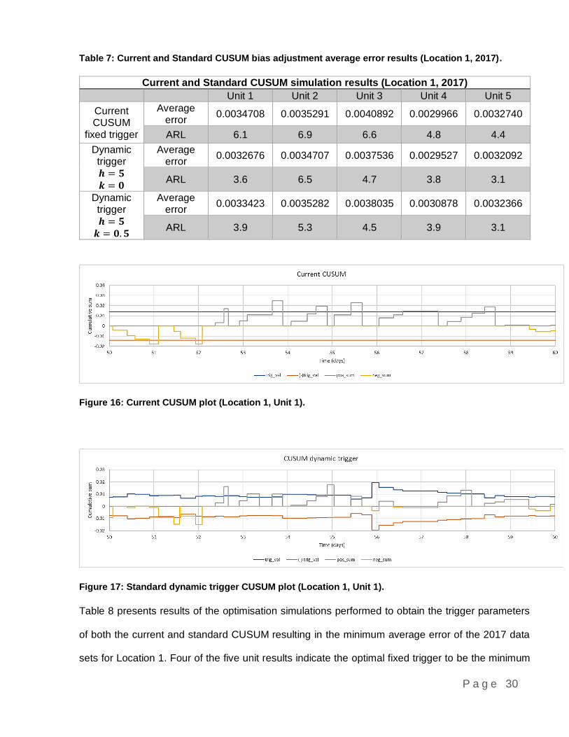
3.2 CUSUM Comparison Analysis

Results obtained from both the current CUSUM and standard CUSUM are presented in Table 7.

Firstly, the dynamic trigger simulation without the slack factor shows a slight reduction in the average

error across all five units. Secondly, the ARL for all units has also decreased. This reduction in the

ARL in an indication of tighter trigger limits. Comparison of the current fixed trigger CUSUM plot in

Figure 16 with the standard CUSUM plot in Figure 17 shows the dynamic trigger to be less than the

fixed trigger for the majority of the 10-day period. The consistency of reduced error and ARL could

be indicating the reduction in average error is due to lower ARL values. Finally, the addition of a

typical slack factor of 𝒌 = 𝟎. 𝟓 to the standard CUSUM results in a consistent slight increase in

average error.

P a g e 30

Table 7: Current and Standard CUSUM bias adjustment average error results (Location 1, 2017).

Current and Standard CUSUM simulation results (Location 1, 2017)

Unit 1 Unit 2 Unit 3 Unit 4 Unit 5

Current CUSUM

fixed trigger

Average error

0.0034708 0.0035291 0.0040892 0.0029966 0.0032740

ARL 6.1 6.9 6.6 4.8 4.4

Dynamic trigger 𝒉 = 𝟓

𝒌 = 𝟎

Average error

0.0032676 0.0034707 0.0037536 0.0029527 0.0032092

ARL 3.6 6.5 4.7 3.8 3.1


𝒌 = 𝟎. 𝟓

Average error

0.0033423 0.0035282 0.0038035 0.0030878 0.0032366

ARL 3.9 5.3 4.5 3.9 3.1

Figure 16: Current CUSUM plot (Location 1, Unit 1).

Figure 17: Standard dynamic trigger CUSUM plot (Location 1, Unit 1).

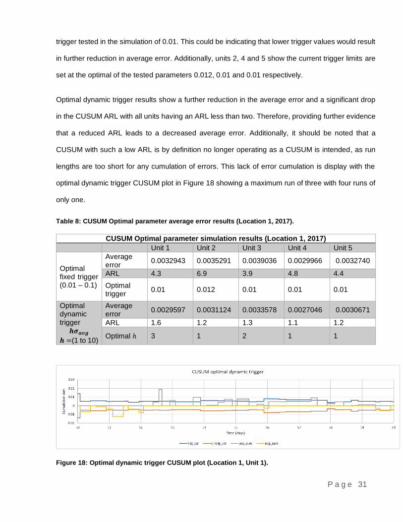
Table 8 presents results of the optimisation simulations performed to obtain the trigger parameters

of both the current and standard CUSUM resulting in the minimum average error of the 2017 data

sets for Location 1. Four of the five unit results indicate the optimal fixed trigger to be the minimum

P a g e 31

trigger tested in the simulation of 0.01. This could be indicating that lower trigger values would result

in further reduction in average error. Additionally, units 2, 4 and 5 show the current trigger limits are

set at the optimal of the tested parameters 0.012, 0.01 and 0.01 respectively.

Optimal dynamic trigger results show a further reduction in the average error and a significant drop

in the CUSUM ARL with all units having an ARL less than two. Therefore, providing further evidence

that a reduced ARL leads to a decreased average error. Additionally, it should be noted that a

CUSUM with such a low ARL is by definition no longer operating as a CUSUM is intended, as run

lengths are too short for any cumulation of errors. This lack of error cumulation is display with the

optimal dynamic trigger CUSUM plot in Figure 18 showing a maximum run of three with four runs of

only one.

Table 8: CUSUM Optimal parameter average error results (Location 1, 2017).

CUSUM Optimal parameter simulation results (Location 1, 2017)


Optimal fixed trigger (0.01 – 0.1)

Average error

0.0032943 0.0035291 0.0039036 0.0029966 0.0032740

ARL 4.3 6.9 3.9 4.8 4.4

Optimal trigger

0.01 0.012 0.01 0.01 0.01

Optimal dynamic trigger

𝒉𝝈𝒂𝒗𝒈

𝒉 =(1 to 10)

Average error

0.0029597 0.0031124 0.0033578 0.0027046 0.0030671

ARL 1.6 1.2 1.3 1.1 1.2

Optimal ℎ 3 1 2 1 1

Figure 18: Optimal dynamic trigger CUSUM plot (Location 1, Unit 1).

P a g e 32

It can be seen in Table 9 that the most considerable reduction in error with respect to the current

CUSUM were obtained via the optimal dynamic trigger simulations. Implementation of the optimal

dynamic trigger results in error reductions ranging from 6.3% to a significant 17.9% where the

maximum improvement of the other simulated methods was only 5.9%. As this optimal trigger

CUSUM is no longer operating as a CUSUM and is providing the minimal average errors indicates

that a CUSUM may not be the best method of bias adjustment for this specific application.

Table 9: CUSUM simulation percentage of average error reduction.

CUSUM simulation results, average error reduction (Location 1, 2017)


Dynamic trigger 𝒉 = 𝟓 𝒌 = 𝟎

Average error

reduction 5.9% 1.7% 8.2% 1.5% 2.0%


𝒌 = 𝟎. 𝟓

Average error

reduction 3.7% 0.03% 7.0% -3.0% 1.1%

Optimal fixed trigger

Average error

reduction 5.1% 0.0% 4.6% 0.0% 0.0%

Optimal dynamic trigger

Average error

reduction 14.7% 11.8% 17.9% 9.7% 6.3%

P a g e 33

Chapter 4: Standard Filter Simulation

Simulations adopting the traditional methods introduced in 1.1.3 were created due to the significant

improvements obtained with the optimal dynamic trigger initiating a bias adjustment nearly every

laboratory sample entry. Firstly, a simulation using the bias calculation of Equation 1-8 is tested again

for all five units of Location 1 using 2017 data sets. This is achieved by setting the filtering term of

Equation 1-9 as 𝑲 = 𝟏. Additionally, as with the CUSUM simulations an optimisation simulation was

ran for each data set to determine the optimal filtering term 𝑲 for each unit.

P a g e 34

Chapter 5: Standard Filter Results

Average error results of the standard error filter simulations using Equation 1-9 are presented in

Table 10. These results show considerable reductions in the average error by merely adjusting the

bias by the established error (𝑲 = 𝟏) every laboratory result entered that passes the limiting

parameters. Comparison of this method to a CUSUM can be by considering this method as having

an ARL of one again supporting the insinuation in Chapter 3.2 that a lower ARL results in decreased

average error.

Table 10: Standard error filter simulation average error results (Location 1, 2017).

Standard error filter simulation average error results (Location 1, 2017)

Error Filter 𝑲(𝒆𝒓𝒓𝒐𝒓)


Total error adjustment

𝑲 = 𝟏

Average error

0.0029789 0.00330351 0.0029885 0.0025344 0.0027288

Optimal error filter

Average error

0.0025922 0.0028276 0.0028876 0.0023946 0.002607

Optimal 𝐾 𝐾 = 0.6 𝐾 = 0.5 𝐾 = 0.6 𝐾 = 0.5 𝐾 = 0.6

Results obtained through establishing the optimal value of 𝑲 for each unit show further error reduction

than simply adjusting the bias by the complete error value. These improved results are an indicator

that the filtering term is reducing the effect of small random and systematic errors in the sampling

process as discussed in the beginning of Chapter 1.1.3. The consistency of the optimal error terms

being 0.6 to 0.5 suggest regular gross errors across all five units. Most importantly is the significant

average error reduction compared with the current CUSUM ranging from 19.9% to 29.4% presented

in Table 11.

P a g e 35

Table 11: Standard error filter, percentage average error reduction results (Location 1, 2017).

Standard error filter simulation, percentage average error reduction (Location 1, 2017)

Error Filter

𝑲(𝒆𝒓𝒓𝒐𝒓) Unit 1 Unit 2 Unit 3 Unit 4 Unit 5

Total error adjustment

𝑲 = 𝟏

Average error

reduction 14.2% 6.4% 26.9% 15.4% 16.7%


Average error

reduction 25.3% 19.9% 29.4% 20.1% 20.4%

Further simulations were performed to provide an understanding of the significant improvements the

error filter shows over the current CUSUM. These simulations used unit 1 of Location 1 as a case

study so that specific bias trends could be analysed. Initially, data obtained between the 50th and

150th day of 2017 was used as it isolated any periods the process or instrumentation were offline as

displayed in the plot of Figure 19. Importantly the error reduction indicated in Table 11 is consistent

with previous results.

Figure 19: Current CUSUM and optimal error filter bias plot (Location 1, unit 1, days 50 to 150 of 2017).

P a g e 36

Table 12: Current CUSUM and optimal error filter bias comparison (Location 1, unit 1, days 50 to 150 of

2017).

Bias adjustment average error comparison Location 1 Unit 1 2017 (days 50-150)

Current CUSUM Filter Optimal Error Filter

Average error 0.0031696 0.0023306

Average error reduction

percentage N/A 26.47%

Focusing in on the 20 day period from days 50 to 70 of Figure 20 shows both methods producing

two different bias trends. During the first ten days, each bias adjustment method results in a ramping

bias indicating the inferential is drifting upwards, and the bias adjustment methods are attempting to

case the BOR. Alternatively, the period between days 60 and 70 show both bias values remaining in

a more steady state which is an indication that the BOR inferred value has minimal drift during that

time frame resulting in minimal bias adjustments required.


P a g e 37


2017).



Average error 0.0036648 0.0022462



The plot in Figure 21 shows the current CUSUM bias lagging the error filter bias during the period of

inferential drift. This lag presented by the current CUSUM is due to the CUSUM only initiating a bias

adjustment when the CUSUM reaches the set trigger value. Whereas the error filter updates the bias

every accepted error calculation enabling the error filter to follow the drifting process value more

closely. The resulting average error reduction of the error filter compared to the current CUSUM

displayed in Table 13 is a very significant 51%. Alternatively, during the period of minimal drift shown

in Figure 22 the error filter produces a slightly less stable bias than the current CUSUM resulting in

an error increase of 10% as shown in Table 15. This is evidence that the CUSUM is optimal during

periods of small drift as this is what it is intended to identify.


P a g e 38


2017).



Average error 0.0061034 0.0029637





2017).



Average error 0.0014527 0.001606


percentage N/A -10.55%

P a g e 39

Chapter 6: Alternative Statistical Filter

Simulation

Due to the benefits of adopting a standard error filter during the significant inferential drift and

alternatively the increase in error during low levels of drift, two alternative bias adjustment methods

are considered. These two methods the Fast Initial Response CUSUM and a Shewhart/ CUSUM

combination attempt to provide increased responsiveness to large shifts while maintaining the

performance of the CUSUM during the minimal drift.

6.1 Fast Initial Response CUSUM

This method as its title suggests was devised to improve the sensitivity of the CUSUM during process

start-up by Lucas and Crosier in 1982 [11].This Fast Initial Response (FIR) is enabled by setting the

initial value of positive and negative summation to a portion their respective trigger limits. By setting

the summation values to this fixed initial setting after a bias adjustment enables the CUSUM to trigger

with a lower ARL during the continued inferential drift. While the CUSUM will rapidly trigger during

these high drift periods the IFR should have minimal effect with low drift as the CUSUM will quickly

settle [13]. The typical IFR of a 50% head-start, where the CUSUM value is reset to half the set trigger

value was adopted for these simulations. The FIR simulations in this project are an adaptation of the

current fixed trigger CUSUM simulations.

P a g e 40

6.2 Shewhart and CUSUM Combination

As indicated in Chapter 1.1.3 the CUSUM was designed to provide an efficient method of detecting

small mean shifts. This offered an alternative to the Shewhart control charts as their performance in

these cases were poor [11]. Alternatively, as the discussed performance of the CUSUM is poor during

large mean shifts. A conventional method of improving the repose of a CUSUM to large shifts is the

combination of a Shewhart control with a CUSUM control. This simulation runs both the CUSUM and

Shewhart control in parallel where a trigger of either will initiate a bias adjustment and reset the

parameters of both. The typical value of 𝟑. 𝟓𝝈𝒂𝒗𝒈 [11] was adopted for the Shewhart trigger and the

typical standard CUSUM trigger of 𝟓𝝈𝒂𝒗𝒈 [11] was also used. Extract of the MTLAB code in Figure

23 shows the implementation of using the average standard deviation as described in Chapter 2.2.4.

Additionally, the slack term of the standard CUSUM was removed from the calculations but setting

parameter 𝒌 to zero due to the findings in Chapter 3.2 indicating increases in average error with the

addition of the slack factor.

Figure 23: Shewhart/CUSUM control calculations MATLAB code.

P a g e 41

Chapter 7: Final Results

Initial results obtained from the FIR CUSUM and the Shewhart/CUSUM simulations are offered in

Table 16. These initial results show the Shewhart/CUSUM method provides lower average errors

than the FIR CUSUM across all five units tested over the 2017 obtained data range. These alternative

simulations were conducted to replicate the error filter results during periods of inferential drift but

also maintain the performance of the current CUSUM during relative inferential stability. Additional

plots for the same periods of drift and stability of the inferential previously used in Chapter 5: Standard

Filter Results are provided in Figure 24 and Figure 25.

Table 16: FIR CUSUM simulation average error results (Location 1, 2017).

FIR CUSUM bias adjustment average error results (Location 1, 2017)


FIR CUSUM

Average error

0.0033075 0.0036216 0.0038952 0.003051 0.0033696

ARL 5.2 7.8 5.1 4.9 4.5

Shewhart & CUSUM

Average error

0.0030500 0.0032248 0.0035266 0.027255 0.0030305

ARL 1.8 1.6 1.7 2.6 1.6

During the period of drift, Figure 24 illustrates that the FIR CUSUM still results in bias lag whereas

the Shewhart/CUSUM adjustment method provides a substantial reduction in the bias lag. Results

presented in Table 17 reiterate the link between reduced average error and reduced bias lag. While

the Shewhart method provides a noteworthy improvement over the current CUSUM, the optimal error

filter still results in the most significant error reduction.

P a g e 42

Figure 24: Alternative bias adjustment plot (Location 1, unit 1, days 50 to 60 of 2017).


Alternative bias adjustment comparison Location 1 Unit 1 2017 (days 50-60)

Current CUSUM

Filter Optimal Error Filter FIR CUSUM

Shewhart & CUSUM

Average error 0.0061034 0.0029637 0.006133 0.0036736


percentage N/A 51.44% -0.48% 39.81%

Periods of minimal drift in the inferred BOR as illustrated in Figure 25 result in both the FIR CUSUM

and the Shewhart/CUSUM simulations providing increased stability over the optimal error filter.

Importantly the Shewhart/CUSUM plot matched very close to the current CUSUM simulated bias.

Average error reduction results in Table 18 for this tested period show a further increase in error from

the FIR CUSUM simulation. Alternatively, the Shewhart/CUSUM simulation provides a slight

improvement over the average error obtained from the optimal error filter. While the

Shewhart/CUSUM simulation provides improvements to the error filter during stability, an average

over both transient and stable inferential as displayed in Figure 26 result in the optimal error filter still

providing the minimum average error (Table 19).

P a g e 43




Current CUSUM


Shewhart & CUSUM

Average error 0.0014527 0.001606 0.0016466 0.0015698


percentage N/A -10.56% -13.35% -8.06%

P a g e 44




Current CUSUM


Shewhart & CUSUM

Average error 0.0031696 0.0023306 0.0036783 0.0025492


percentage N/A 26.47% -16.05% 19.57%

The final results of all simulated bias adjustment methods for Location 1 using PHD data from the

2017 period indicated in Table 1 are contained in Table 20. These results show the optimal error filter

providing the highest magnitude of error reduction for all five units. The current CUSUM, as well as

optimal error filter results for Location 2 and Location 3, are displayed in Table 21 and Table 22 again

showing the uniformity of the filter parameter 𝑲 within each location. Significant improvement over

the current adjustment method is shown to be consistent across the other two locations units as

displayed in Table 23. This continued improvement is due to all three locations exhibiting cyclic drift

of the inferred BOR as illustrated in Figure 27. It is also evident that the smaller improvements

obtained during simulations for Location 2 is due to the observed less significant drift.

P a g e 45

Table 20: Complete average error reduction results for all simulations (Location 1, 2017).

Error reduction percentage of all simulated bias adjustment methods (Location 1, 2017)

Bias adjustment method



𝒌 = 𝟎

5.9% 1.7% 8.2% 1.5% 2.0%


𝒌 = 𝟎. 𝟓 3.7% 2.6% 7.0% -3.0% 1.1%

Optimal fixed trigger 5.1% 0.0% 4.6% 0.0% 0.0%

Optimal dynamic trigger 𝒌 = 𝟎

14.7% 11.8% 17.9% 9.7% 6.3%

Error filter

𝑲 = 𝟏 14.2% 6.4% 26.9% 15.4% 16.7%

Optimal error filter 25.3% 19.9% 29.4% 20.1% 20.4%

FIR CUSUM 4.7% -2.6 4.7 -1.8 -2.9

Shewhart/CUSUM 12.1% 8.6% 13.8% 9.0% 7.4%

Table 21: Location 2 simulation results 2017.

Current CUSUM and Optimal error filter simulation average error results (Location 2, 2017)


Current CUSUM

Average error

0.0038371 0.0030270 0.0030144 0.0032547 0.0033413


Average error

0.0032144 0.0026352 0.0024994 0.0028207 0.0027547

Optimal 𝐾 𝐾 = 0.4 𝐾 = 0.4 𝐾 = 0.5 𝐾 = 0.4 𝐾 = 0.4

Table 22: Location 3 simulation results 2017.

Current CUSUM and Optimal error filter simulation average error results (Location 3, 2017)

Unit 1 Unit 2

Current CUSUM Average error 0.0045128 0.0043602

Optimal error filter Average error 0.0035917 0.0035242

Optimal 𝐾 𝐾 = 0.6 𝐾 = 0.6

P a g e 46

Table 23: Optimal error filter average error reduction results (all locations).

Optimal error filter annual average error reduction

Site Year Unit 1 Unit 2 Unit 3 Unit 4 Unit 5

Location 1 2017 25.31% 19.88% 29.38% 20.09% 23.84%

Location 2 2017 16.23% 12.94% 17.08% 13.33% 17.56%

Location 3 2017 20.41% 19.17% N/A N/A N/A

Figure 27: All three locations bias comparison (2017).

P a g e 47

Chapter 8: Discussion

The intended purpose of simulating an alternative SSI was to enable consistent results over a

fluctuating process noise variance alleviating the need to adjust the limiting parameter over time.

While Figure 14 indicates evidence of this being the case the level of process noise could affect error

calculations resulting in incorrect bias adjustment. This coupled with the lagging nature of the R-

statistic resulting in type I and type II errors shows little if any benefit of replacing the current standard

deviation method of SSI.

The bias adjustment simulation results presented in this Thesis use the laboratory analysis results

as the reference for calculating the inferred BOR error. This assumption of zero error in the laboratory

results has been made for two reasons. Firstly, the limiting parameters of Table 2 help to remove

most of the outlying errors. Secondly, the primary performance indicator of the average error

reduction uses the current CUSUM results as this error reduction reference. This results in the gross

and random errors present after the limiting parameters being present in both the current CUSUM

and comparing method calculations. Therefore, standardising the error reductions from these

unknown errors.

Initial CUSUM simulation results summarised in Table 9 show consistent error reduction across all

tested units when the standard CUSUM method of calculating the trigger value (Equation 2-5) is

implemented. This reduction in error coincides with decreasing ARL results and tightening of the

trigger limits as indicated in Table 7 and Figure 17 respectively. A standard CUSUM usually

incorporates a slack factor 𝒌𝝈 to reduce the effects of noise by only using errors greater than 𝒌𝝈 in

the CUSUM calculation. While the typical value for this slack factor is documented to be 𝒌 = 𝟎. 𝟓 [11]

simulated results for this application cause a reduction in the improvements made with the standard

dynamic trigger. These negative results suggest the error noise required to be removed from the

calculations to provide an improvement in the results is less than 𝟎. 𝟓𝝈 and can be considered

insignificant for the purposes of this investigation.

P a g e 48

Of most interest when comparing the simulated CUSUM methods is the trend of reduced average

error with lower ARL values. We can see that the optimisation simulations for both the fixed and

dynamic triggers while designed to establish the triggers resulting in minimum average error drive

these trigger values down. These diminishing values are evident in the results of Table 8 indicating

that the majority of optimal trigger parameters are found to be the lowest value tested. These low

trigger values directly reduce the ARL of the CUSUM as illustrated in Figure 18 and cause the

CUSUM to operate outside the definitions of a CUSUM. This initial analysis indicates that a CUSUM

may not be the optimal solution for this application.

Simulating the traditional method of correcting the bias by the full magnitude of the error provided

results similar to those obtained with the optimal dynamic trigger (Table 20). These results are

unsurprising due to the optimal dynamic trigger for each unit provided an ARL less than two which is

similar to adding the error to the bias nearly every approved laboratory result as the case is with the

traditional method.

The significant and consistent improvement in the bias-corrected inferential obtained with the use of

the optimal error filter is of great interest. Research suggests even an error filtering term added to

the traditional method of bias adjustment leads to results that are predominantly worse than when a

CUSUM is implemented [9]. Further investigation shows significant drift in the inferred value of the

BOR resulting in the bias calculated with a CUSUM lagging due to the number of samples required

for the CUSUM to trigger the required bias adjustment. This is an inherent issue of a CUSUM as they

are designed to monitor small mean shifts and provide poor performance in detecting large shifts

[11]. Due to this and the inherent cyclic drift of the current inferential displayed in Figure 27 the optimal

error filter while not recommended in most cases provides significant reductions in the average error

for this application.

Focused analysis indicates periods when the current CUSUM performs better than the optimal error

filter. These periods as displayed in Figure 22 are indicative of minimal drift which is the application

P a g e 49

a CUSUM is intended for. While these periods exist, the majority of the inferential is transient in

nature. Two alternative CUSUM methods were simulated in an attempt to combine the positive

results of the error filter during transient periods and the CUSUM during periods of relatively stable

inferred BOR values. Of these two methods, the FIR CUSUM showed little if any improvement in the

results of the error filter. Alternatively, the combination of a Shewhart and CUSUM calculation showed

promise by only reducing the improvements slightly during transient periods but also resulting in a

small improvement during stability. While this Shewhart/CUSUM method is an option for possible

consideration, the overall average error reduction for each unit of Location 1 (Table 20) obtained with

the optimal error filter is considerably more significant. Additionally, the optimal error filter shows

consistently significant results across all three locations as indicated in Table 23.

P a g e 50

Chapter 9: Conclusion

Simulation of the R-statistic was implemented in an attempt to improve the method of SSI used to

establish when an error calculation should be made. The R-statistic being a ratio of two different

methods of determining the variance of sequential data points provides minimal difference of results

during fluctuations in process noise. This was proven but what was not anticipated was this very

attribute producing type II errors during noise levels considered too high for error calculations to be

accurate. For this reason and the increased type I and II errors resulting from the lagging nature of

this method, the R-statistic is not recommend without further development.

Literature research shows that in the majority of cases the use of a CUSUM algorithm produces lower

errors than the traditional error filter when used to automatically adjust an inferential bias [9]. This is

due to the error filter introducing random errors caused by the sampling process into the inferred

calculation. While this has been indicated to be the case during relatively stable periods of the inferred

value the majority of the tested inferential values are more transient than stable. This transient nature

of the inferred BOR indicates a nonlinearity in the conductivity and BOR relationship and or the

requirement for additional process variables to be included in the BOR calculation. Therefore, it is

recommended to investigate the current inferential calculations and identify any modifications

required.

The substantial reductions in the average error across all twelve units obtained with the optimal error

filter simulations suggest any random sampling errors are of less significance than the inferred bias

error introduced by the lagging CUSUM. Therefore, the second recommendation is to initially

implement the optimal error filter to the control system of a number of the units to assess its

performance online. Implementation of the optimal error filter will provide instant improvements in the

inferred BOR enabling increased control capabilities. Reassessment of the most appropriate bias

adjustment method after any alternation to the inferential calculation would ensure the optimal

method of bias adjustment is maintained.

P a g e 51

Chapter 10: References

[1] D. Donaldson and B. Raahauge, Essential Readings in Light Metals, Alumina and Bauxite, New

Jersey: John Wiley & Sons, Incorporated, 2013.

[2] K. R. Seechattan, "Bayer Process Chemistry," Linden, 2010.

[3] B. R. Limited, "What is Bauxite?," IRM, 2018. [Online]. Available:

http://www.bauxiteresources.com.au/irm/content/what-is-bauxite.aspx?RID=318. [Accessed 25

09 2017].

[4] S. Cao and R. R. Rhinehart, "An efficient method for on-line identification of steady state,"

Journal of Process Control, vol. 5, no. 6, pp. 363-374, 1995.

[5] T. Huang, "Steady State and Transient State Identification in an Industrial Process," ProQuest,

New Jersey, 2010.

[6] M. Kim, S. H. Yoon, P. A. Domanski and W. V. Payne, "Design of a steady-state detector for

fault detection and diagnosis of a residential air conditioner," International Journal of

Refrigeration, vol. 31, pp. 790-799, 2008.

[7] G. Jubien and G. Bihary, "Variation standard deviation is best measure of steady state,"

CONTROL for the process Industries, vol. 3, no. 11, p. 64, 1994.

[8] V. Vasyutynskyy, Passive monitoring of control loops in building automation, 2005.

[9] M. J. King, "How to lose money with inferential properties," Whitehouse Consulting, Isle of

Wight, UK, 2004.

[10] M. j. King, Statistics for Process Control Engineers: A Practical Approach, John Wiley & Sons

Ltd., 2017.

[11] D. C. Montgomery, Introduction to Statistical Quality Control, Hoboken, NJ 07030: John Wiley

& Sons, Inc., 2009.

[12] P. Qiu, Introduction to Statistical Process Control, Boca Raton, Florida: CRC Press, 2014.

P a g e 52

[13] E. R. Ott, E. G. Schilling and D. V. Neubauer, Process Quality Control: Troubleshooting and

Interpretation of Data, Hew York: McGraw-Hill, 2000.

[14] R. D. Hond, I. Hiralal and A. Rijkeboer, "Alumina Yield in the Bayer Process; Past, Present and

Prospects," The Minerals, Metals and Materials Society, 2007.

P a g e 53

Appendix

A.1 Reference Documentation Links

Honeywell - DOC4000 User Guide Version 4.0

Introduces the required tools and necessary information in the navigation of the DOC4000

automation Genome enabling access to the TDC3000 control language and tags required for the

current system analysis.

Honeywell - TDC3000 Engineers Reference Manual

Provides information enabling insight into the current control system used in the BOR bias

adjustment.

Honeywell – Control Language Application Module Reference Manual

Complete reference manual on the control language used in the current control system used for the

bias adjustment program.

Honeywell – Uniformance Process Studio User Guide

User guide providing method for searching complete tags required for PHD data extraction.

Honeywell – Uniformance Excel Companion (Profit Embedded PHD) User Guide

User guide for the Microsoft Excel add-in required for data extraction from the PHD.

MATLAB Documentation - MathWorks

Link to MathWorks web page with access to MATLAB code examples and reference documentation.

https://www.honeywellprocess.com/library/marketing/notes/DOC4000_User_Guide.pdf

http://ftp.ruigongye.com/200807/engineersreferencemanual.pdf

https://www.honeywellprocess.com/library/marketing/product-manuals/AM27-510.pdf

http://hw.server.tracorp.com/courses/ac/5768/UPSUserGuide_pim5001.pdf

https://www.honeywellprocess.com/library/marketing/product-manuals/AP20-510PS.pdf

https://au.mathworks.com/help/matlab/

P a g e 54

A.2 Simulation Code

A2.1 Steady State Identification Simulation code

%Import data from Excel %Manually enter "filename", "sheet" and "###_xlRange" variables. filename='LOC1_BOR_20170807-20170904.xlsx'; sheet='U1 BOR'; RawData_xlRange='B14:B40334'; StdData_xlRange='J14:J40334'; ErrorData_xlRange='I14:I40334'; LabData_xlRange='F14:F40334'; TimeStamp_xlRange='A14:A40334'; SampleTime_xlRange='E14:E40334'; AvgData_xlRange='G14:G40334';

RawData = xlsread(filename, sheet, RawData_xlRange); StdData=xlsread(filename, sheet, StdData_xlRange); ErrorData=xlsread(filename, sheet, ErrorData_xlRange); LabData=xlsread(filename, sheet, LabData_xlRange); [num,text,TimeStamp]=xlsread(filename, sheet, TimeStamp_xlRange); [num2,text2,SampleTime]=xlsread(filename, sheet, SampleTime_xlRange); AvgData=xlsread(filename, sheet, AvgData_xlRange);

Dsize=size(RawData); Dsize=Dsize(1,1); StdHi=0.005; % Ensure correct setting for location and unit. StdLow=0; ErrorLim=0.015;

% Subarray adjustment subtime=Dsize/2; subsize=subtime-2; % subtime=36013 + 2; % subsize=300;

subRawData=RawData(subtime-subsize:subtime+subsize,1); subStdData=StdData(subtime-subsize:subtime+subsize,1); subErrorData=ErrorData(subtime-subsize:subtime+subsize,1); subLabData=LabData(subtime-subsize:subtime+subsize,1); subTimeStamp=TimeStamp(subtime-subsize:subtime+subsize,1); subSampleTime=SampleTime(subtime-subsize:subtime+subsize,1); subAvgData=AvgData(subtime-subsize:subtime+subsize,1);

Error=[subErrorData]; Std=[subStdData]; Lab=[subLabData]; AVG=[subAvgData];

datasize=size(subRawData); datasize=datasize(1,1); t=1:datasize;

%data filter variables dataF=[RawData(subtime-subsize)];

P a g e 55

lam1=0.2; %variance estimate No.1 lam2=0.1; v2F=[lam2*((RawData(subtime-subsize)-(RawData(subtime-subsize-1))).^2)]; %variance estimate No.2 lam3=0.1; sigF=[lam3*((RawData(subtime-subsize)-(RawData(subtime-subsize-1))).^2)];

% Initiate variables R=[1]; Rhi=5; Rlow=0; TestR=[1]; NewSSI=[0]; CurrentSSI=[0]; LabSample=[min(RawData)]; NewSSICount=0; CurrentSSICount=0; LabSampleCount=0; ShiftCount=0; avg=[subRawData]; AvgTime=10; i=1; TempTime=' '; SD=[0];

while i<datasize i=i+1; %data filter dataF(i)=lam1*subRawData(i)+(1-lam1)*dataF(i-1); %variance estimate No.1 v2F(i)=lam2*((subRawData(i)-(dataF(i-1))).^2)+(1-lam2)*v2F(i-1); %variance estimate No.2 sigF(i)=lam3*((subRawData(i)-subRawData(i-1)).^2)+(1-lam3)*sigF(i-1); %ratio of variance #1 & #2 R(i)=((2-lam1)*v2F(i))/sigF(i);

%Raw data average if i>12&&i<datasize-12 avg(i)=mean(subRawData(i-AvgTime:i+AvgTime)); SD(i)=std(subRawData(i-AvgTime:i+AvgTime)); else avg(i)=subRawData(i); SD(i)=0; end

% New steady state identifier if R(i)>Rlow&&R(i)<Rhi NewSSI(i)=1; else NewSSI(i)=0; end

end i=1; while i<datasize i=i+1;

P a g e 56

%Test for for new laboratory result if strcmp(subSampleTime(i),subSampleTime(i-1))==0 n=1;

% Zero "LabSampleTime" seconds LabSampleCount=LabSampleCount+1; TempTime=char(subSampleTime(i)); TempTime=fliplr(TempTime); TempTime(4:6)='00:'; TempTime=fliplr(TempTime);

%Match "LabSampleTime" with "TimeStamp" to align data while n<datasize n=n+1; if strcmp(TempTime,subTimeStamp(n))==1 Error(n:datasize)=subErrorData(i); Std(n:datasize)=subStdData(i); Lab(n:datasize)=subLabData(i); AVG(n:datasize)=subAvgData(i); ShiftCount=ShiftCount+1; ShiftSampleTime=char(subSampleTime(i)); ShiftTimeStamp=char(subTimeStamp(i)); end end else Error(i)=Error(i-1); Std(i)=Std(i-1); Lab(i)=Lab(i-1); AVG(i)=AVG(i-1); end end i=1; while i<datasize i=i+1; % Current steady state identifier Error(i)=abs(Error(i)); if Std(i)>StdLow&&Std(i)<StdHi CurrentSSI(i)=1; else CurrentSSI(i)=0; end

if Lab(i)~=Lab(i-1) LabSample(i)=Lab(i); TestR(i)=R(i); if R(i)>Rlow&&R(i)<Rhi NewSSICount=NewSSICount+1; end

if Std(i)>StdLow&&Std(i)<StdHi CurrentSSICount=CurrentSSICount+1; end

else LabSample(i)=min(RawData); TestR(i)=TestR(i-1);

P a g e 57

end

% Display conflicting SSI triggers if Lab(i)~=Lab(i-1)&&CurrentSSI(i)==1&&NewSSI(i)~=1 Time=char(subTimeStamp(i)); fprintf('NewSSI = TS and CurrentSSI = SS at time = %s or

t(%d).\n',Time,t(i)); end if Lab(i)~=Lab(i-1)&&CurrentSSI(i)==0&&NewSSI(i)~=0 Time=char(subTimeStamp(i)); fprintf('CurrentSSI = TS and NewSSI = SS at time = %s or

t(%d).\n',Time,t(i)); end end

%Plot PHD BOR, calculated standard deviation and R-statistic ratio figure(1) subplot(3,1,1); plot(t,subRawData); ylim([0.74,0.8]); title('Steady State Identifier Test Data'); legend('Raw Data'); ylabel('BOR');

subplot(3,1,2); plot(t,SD); ylim([0.0,0.015]); legend('Standard Deviation'); ylabel('std');

subplot(3,1,3); plot(t,R); legend('Variance Ratio'); ylabel('var1/var2'); xlabel('Time (min)');

%Display count results fprintf('File - %s : Unit - %s.\n',filename,sheet); CurrentSSIPercent=CurrentSSICount/LabSampleCount*100; NewSSIPercent=NewSSICount/LabSampleCount*100; T=table(LabSampleCount,CurrentSSICount,NewSSICount,CurrentSSIPercent,NewSSIPerce

nt)

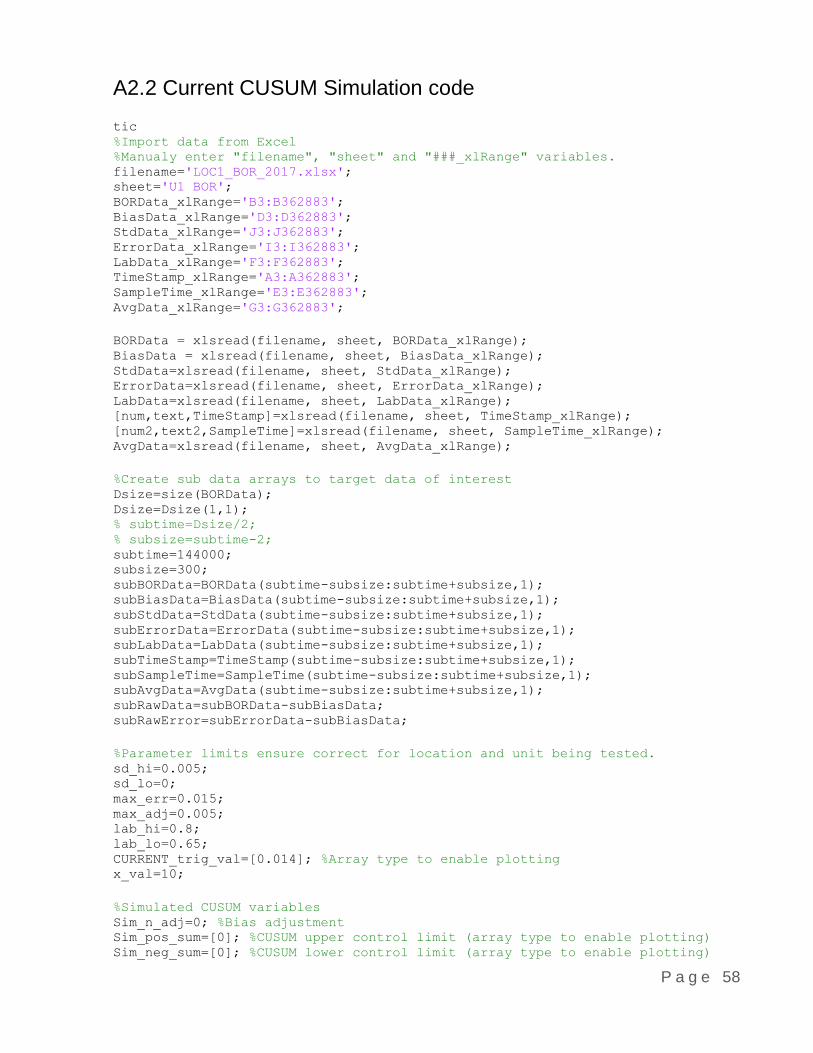
P a g e 58

A2.2 Current CUSUM Simulation code

tic %Import data from Excel %Manualy enter "filename", "sheet" and "###_xlRange" variables. filename='LOC1_BOR_2017.xlsx'; sheet='U1 BOR'; BORData_xlRange='B3:B362883'; BiasData_xlRange='D3:D362883'; StdData_xlRange='J3:J362883'; ErrorData_xlRange='I3:I362883'; LabData_xlRange='F3:F362883'; TimeStamp_xlRange='A3:A362883'; SampleTime_xlRange='E3:E362883'; AvgData_xlRange='G3:G362883';

BORData = xlsread(filename, sheet, BORData_xlRange); BiasData = xlsread(filename, sheet, BiasData_xlRange); StdData=xlsread(filename, sheet, StdData_xlRange); ErrorData=xlsread(filename, sheet, ErrorData_xlRange); LabData=xlsread(filename, sheet, LabData_xlRange); [num,text,TimeStamp]=xlsread(filename, sheet, TimeStamp_xlRange); [num2,text2,SampleTime]=xlsread(filename, sheet, SampleTime_xlRange); AvgData=xlsread(filename, sheet, AvgData_xlRange);

%Create sub data arrays to target data of interest Dsize=size(BORData); Dsize=Dsize(1,1); % subtime=Dsize/2; % subsize=subtime-2; subtime=144000; subsize=300; subBORData=BORData(subtime-subsize:subtime+subsize,1); subBiasData=BiasData(subtime-subsize:subtime+subsize,1); subStdData=StdData(subtime-subsize:subtime+subsize,1); subErrorData=ErrorData(subtime-subsize:subtime+subsize,1); subLabData=LabData(subtime-subsize:subtime+subsize,1); subTimeStamp=TimeStamp(subtime-subsize:subtime+subsize,1); subSampleTime=SampleTime(subtime-subsize:subtime+subsize,1); subAvgData=AvgData(subtime-subsize:subtime+subsize,1); subRawData=subBORData-subBiasData; subRawError=subErrorData-subBiasData;

%Parameter limits ensure correct for location and unit being tested. sd_hi=0.005; sd_lo=0; max_err=0.015; max_adj=0.005; lab_hi=0.8; lab_lo=0.65; CURRENT_trig_val=[0.014]; %Array type to enable plotting x_val=10;

%Simulated CUSUM variables Sim_n_adj=0; %Bias adjustment Sim_pos_sum=[0]; %CUSUM upper control limit (array type to enable plotting) Sim_neg_sum=[0]; %CUSUM lower control limit (array type to enable plotting)

P a g e 59

Sim_pos_cnt=0; %CUSUM upper summation Sim_neg_cnt=0; %CUSUM lower summation

% Initiate data arrays and variables SimAvg=[AVG]; SimAv=AVG(1); SimStd=[subStdData]; SimSd=Std(1); datasize=size(subBORData); datasize=datasize(1,1); t=1:datasize; LabSampleCount=0; TempTime=' ';

SimErrorArray=[Error]; ErrSum=0; SimErrSum=0; RawErrSum=0; ARLsum=0; ErrCnt=0; RawErrCnt=0; SimErrCnt=0; SimTrigCnt=0; TestSampleCount=0;

SimBias=[subBiasData(1)]; SimData=[subBORData]; SimAvg=AVG;

i=1; while i<datasize i=i+1; CURRENT_trig_val(i)=CURRENT_trig_val(i-1); Sim_pos_sum(i)=Sim_pos_sum(i-1); Sim_neg_sum(i)=Sim_neg_sum(i-1);

%Test for new laboratory result if strcmp(subSampleTime(i),subSampleTime(i-1))==0 %Set Sample Time seconds to :00 TempTime=char(subSampleTime(i)); TempTime=fliplr(TempTime); TempTime(4:6)='00:'; TempTime=fliplr(TempTime); TestSampleCount=TestSampleCount+1;

%Find online data at lab sample time n=1; while n<datasize n=n+1; if strcmp(TempTime,subTimeStamp(n))==1 if n>10 TestData=[SimData(n-x_val:n+x_val)]; else TestData=[SimData(1:n+x_val)]; end SimAv=mean(TestData); SimSd=std(TestData);

P a g e 60

SimErr=subLabData(i+2)-SimAv; SimErrorArray(i)=subLabData(i+2)-SimAv; RawErr=subLabData(i+2)-RawAVG(i); LabSampleCount=LabSampleCount+1;

%Average error calculations if abs(SimErr)<max_err&&SimSd<sd_hi&&SimSd>sd_lo&&...

subLabData(i)<lab_hi&&subLabData(i)>lab_lo&&subLabData(i+2)==subLabData(i+3) RawErrSum=RawErrSum+abs(RawErr); RawErrCnt=RawErrCnt+1; end

%CUSUM calculation if parameters are within limits if abs(SimErr)<max_err&&SimSd<sd_hi&&SimSd>sd_lo&&....

subLabData(i)<lab_hi&&subLabData(i)>lab_lo&&subLabData(i+2)==subLabData(i+3) Sim_pos_sum(i)=max(0,Sim_pos_sum(i-1)+SimErr); Sim_neg_sum(i)=min(0,Sim_neg_sum(i-1)+SimErr); SimErrSum=SimErrSum+abs(SimErr); SimErrCnt=SimErrCnt+1; else Sim_pos_sum(i)=Sim_pos_sum(i-1); Sim_neg_sum(i)=Sim_neg_sum(i-1); end

%Bias adjustment calculation if Sim_pos_sum(i-1)>CURRENT_trig_val(i) Sim_n_adj=Sim_pos_sum(i)/(Sim_pos_cnt+1); SimTrigCnt=SimTrigCnt+1; ARLsum=ARLsum+Sim_pos_cnt; elseif Sim_neg_sum(i-1)<((-1)*CURRENT_trig_val(i)) Sim_n_adj=Sim_neg_sum(i)/(Sim_neg_cnt+1); SimTrigCnt=SimTrigCnt+1; ARLsum=ARLsum+Sim_neg_cnt; else Sim_n_adj=0; end

%CUSUM reset if Sim_pos_sum(i-1)>CURRENT_trig_val(i)||Sim_neg_sum(i-1)<((-

1)*CURRENT_trig_val(i)) Sim_pos_cnt=0; Sim_neg_cnt=0; Sim_pos_sum(i)=0; Sim_neg_sum(i)=0; elseif Sim_pos_sum(i-1)<CURRENT_trig_val(i)&&Sim_neg_sum(i-

1)>((-1)*CURRENT_trig_val(i)) Sim_pos_cnt=Sim_pos_cnt+1; Sim_neg_cnt=Sim_neg_cnt+1; end if Sim_pos_sum(i)==0 Sim_pos_cnt=0; end if Sim_neg_sum(i)==0 Sim_neg_cnt=0; end

P a g e 61

%Adjustment limit if Sim_n_adj>max_adj Sim_n_adj=max_adj; end if Sim_n_adj<((-1)*max_adj) Sim_n_adj=((-1)*max_adj); end

%exit while loop break end SimAvg(i)=SimAv; SimStd(i)=SimSd; end

else %Index arrays keeping last value if no change. SimErrorArray(i)=SimErrorArray(i-1); Sim_n_adj=0; SimAvg(i)=SimAvg(i-1); SimStd(i)=SimStd(i-1); end

%Update bias and bias corrected BOR SimBias(i)=SimBias(i-1)+Sim_n_adj; SimData(i)=subRawData(i)+SimBias(i); end

%Calculate and display average errors SimAvEr=SimErrSum/SimErrCnt; RawAvEr=RawErrSum/RawErrCnt; ARL_Avg=ARLsum/SimTrigCnt; T=table(SimAvEr,RawAvEr,SimTrigCnt,LabSampleCount,ARL_Avg)

%Display file and parameters used fprintf('File - %s : Unit - %s.\n',filename,sheet); fprintf('Current CUSUM Parameters: trig_val=%d,

max_error=%d\n',CURRENT_trig_val(1),max_err);

%Display program run time runtime=toc; fprintf('Program runtime = %0.0f minutes.\n',runtime/60);

P a g e 62

A2.3 Standard CUSUM Simulation code

tic %Import data from Excel %Manually enter "filename", "sheet" and "###_xlRange" variables. filename='LOC1_BOR_2017.xlsx'; sheet='U1 BOR'; BORData_xlRange='B3:B362883'; BiasData_xlRange='D3:D362883'; StdData_xlRange='J3:J362883'; ErrorData_xlRange='I3:I362883'; LabData_xlRange='F3:F362883'; TimeStamp_xlRange='A3:A362883'; SampleTime_xlRange='E3:E362883'; AvgData_xlRange='G3:G362883';



%Parameter limits ensure correct for location and unit being tested. sd_hi=0.005; sd_lo=0; max_err=0.015; max_adj=0.005; lab_hi=0.8; lab_lo=0.65; Sim_trig_val=[0.014]; x_val=10;

%Simulated CUSUM variables Sim_n_adj=0; Sim_pos_sum=[0]; Sim_neg_sum=[0];

P a g e 63

Sim_pos_cnt=0; Sim_neg_cnt=0; k=0.5; % Slack factor parameter h=5; % Dynamic trigger parameter


ErrSum=0; SimErrSum=0; RawErrSum=0; SimSdSum=0; ErrCnt=0; RawErrCnt=0; SimErrCnt=0; SimTrigCnt=0; SimSdCnt=0; ARLsum=0;

SimBias=[subBiasData(1)]; SimData=[subBORData]; Simavg=AVG;

i=1;

while i<datasize i=i+1; Sim_trig_val(i)=Sim_trig_val(i-1); Sim_pos_sum(i)=Sim_pos_sum(i-1); Sim_neg_sum(i)=Sim_neg_sum(i-1);

%Test for new laboratory result if strcmp(subSampleTime(i),subSampleTime(i-1))==0 %Set Sample Time seconds to :00 TempTime=char(subSampleTime(i)); TempTime=fliplr(TempTime); TempTime(4:6)='00:'; TempTime=fliplr(TempTime);

%Find online data at lab sample time n=1; while n<datasize n=n+1; if strcmp(TempTime,subTimeStamp(n))==1 TestData=[SimData(n-x_val:n+x_val)]; SimAv=mean(TestData); SimSd=std(TestData); SimErr=subLabData(i+2)-SimAv; RawErr=subLabData(i+2)-RawAVG(i);

P a g e 64

ErrData=subLabData(i+2)-subAvgData(i+2); LabSampleCount=LabSampleCount+1;

% Average error calculations if

abs(ErrData)<max_err&&SimSd<sd_hi&&SimSd>sd_lo&&subLabData(i)<lab_hi&&subLabData

(i)>lab_lo&&subLabData(i+2)==subLabData(i+3) ErrCnt=ErrCnt+1; ErrSum=ErrSum+abs(ErrData); end if

abs(SimErr)<max_err&&SimSd<sd_hi&&SimSd>sd_lo&&subLabData(i)<lab_hi&&subLabData(

i)>lab_lo&&subLabData(i+2)==subLabData(i+3) RawErrSum=RawErrSum+abs(RawErr); RawErrCnt=RawErrCnt+1; end

%CUSUM calculation if parameters are within limits if


i)>lab_lo&&subLabData(i+2)==subLabData(i+3) SimSdCnt=SimSdCnt+1; SimSdSum=SimSdSum+SimSd; SimSdAvg=SimSdSum/SimSdCnt; Sim_trig_val(i)=h*SimSdAvg; Sim_pos_sum(i)=max(0,((subLabData(i+2)-(k*SimSd))-

SimAv)+Sim_pos_sum(i-1)); Sim_neg_sum(i)=min(0,((subLabData(i+2)-(k*SimSd))-

SimAv)+Sim_neg_sum(i-1)); SimErrSum=SimErrSum+abs(SimErr); SimErrCnt=SimErrCnt+1; else Sim_pos_sum(i)=Sim_pos_sum(i-1); Sim_neg_sum(i)=Sim_neg_sum(i-1); Sim_trig_val(i)=Sim_trig_val(i-1); end

%Bias adjustment calculation if Sim_pos_sum(i-1)>Sim_trig_val(i) Sim_n_adj=Sim_pos_sum(i)/(Sim_pos_cnt+1); SimTrigCnt=SimTrigCnt+1; ARLsum=ARLsum+Sim_pos_cnt; elseif Sim_neg_sum(i-1)<((-1)*Sim_trig_val(i)) Sim_n_adj=Sim_neg_sum(i)/(Sim_neg_cnt+1); SimTrigCnt=SimTrigCnt+1; ARLsum=ARLsum+Sim_neg_cnt; else Sim_n_adj=0; end

%CUSUM reset if Sim_pos_sum(i-1)>Sim_trig_val(i)||Sim_neg_sum(i-1)<((-

1)*Sim_trig_val(i)) Sim_pos_cnt=0; Sim_neg_cnt=0; Sim_pos_sum(i)=0; Sim_neg_sum(i)=0; SimSdCnt=0;

P a g e 65

SimSdSum=0; elseif Sim_pos_sum(i-1)<Sim_trig_val(i)&&Sim_neg_sum(i-1)>((-

1)*Sim_trig_val(i)) Sim_pos_cnt=Sim_pos_cnt+1; Sim_neg_cnt=Sim_neg_cnt+1; end if Sim_pos_sum(i)==0 Sim_pos_cnt=0; end if Sim_neg_sum(i)==0 Sim_neg_cnt=0; end


%exit while loop break

end SimAvg(i)=SimAv; SimStd(i)=SimSd; end

else %Index arrays keeping last value if no change. Sim_n_adj=0; SimAvg(i)=SimAvg(i-1); SimStd(i)=SimStd(i-1); end


%Calculate and display average errors AvEr=ErrSum/ErrCnt; SimAvEr=SimErrSum/SimErrCnt; RawAvEr=RawErrSum/RawErrCnt; ARL=ARLsum/SimTrigCnt; T=table(AvEr,SimAvEr,RawAvEr,SimTrigCnt,LabSampleCount,ARL)

%Display file and parameters used fprintf('File - %s : Unit - %s.\n',filename,sheet); fprintf('New CUSUM Parameters: k=%d, h=%d\n',k,h);


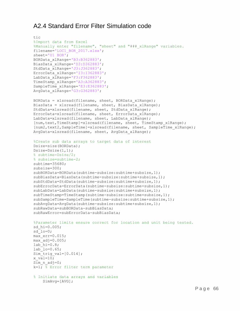
P a g e 66

A2.4 Standard Error Filter Simulation code




%Parameter limits ensure correct for location and unit being tested. sd_hi=0.005; sd_lo=0; max_err=0.015; max_adj=0.005; lab_hi=0.8; lab_lo=0.65; Sim_trig_val=[0.014]; x_val=10; Sim_n_adj=0; k=1; % Error filter term parameter

% Initiate data arrays and variables SimAvg=[AVG];

P a g e 67

SimAv=AVG(1); SimStd=[subStdData]; SimSd=Std(1); datasize=size(subBORData); datasize=datasize(1,1); t=1:datasize; LabSampleCount=0; TempTime=' ';

SimError=[Error]; RawError=[Error]; ErrSum=0; SimErrSum=0; RawErrSum=0; ErrCnt=0; RawErrCnt=0; SimErrCnt=0; SimTrigCnt=0;


i=1; while i<datasize i=i+1; Sim_trig_val(i)=Sim_trig_val(i-1);


%Find online data at lab sample time n=1; while n<datasize n=n+1; if strcmp(TempTime,subTimeStamp(n))==1&&n>10 TestData=[SimData(n-x_val:n+x_val)]; SimAv=mean(TestData); SimSd=std(TestData); SimErr=subLabData(i+2)-SimAv; SimError(i)=subLabData(i+2)-SimAv; RawError(i)=subLabData(i+2)-RawAVG(i); RawErr=subLabData(i+2)-RawAVG(i); ErrData=subLabData(i+2)-subAvgData(i+2); LabSampleCount=LabSampleCount+1;

%Average error calculations if


(i)>lab_lo&&subLabData(i+2)==subLabData(i+3) ErrCnt=ErrCnt+1; ErrSum=ErrSum+abs(ErrData);

P a g e 68

end if


i)>lab_lo&&subLabData(i+2)==subLabData(i+3) RawErrSum=RawErrSum+abs(RawErr); RawErrCnt=RawErrCnt+1; end

%CUSUM calculation if error and std are within limits if


i)>lab_lo&&subLabData(i+2)==subLabData(i+3) Sim_n_adj=k*SimErr; SimErrSum=SimErrSum+abs(SimErr); SimErrCnt=SimErrCnt+1; else Sim_n_adj=0; end



else %Index arrays keeping last value if no change. SimError(i)=SimError(i-1); RawError(i)=RawError(i-1); Sim_n_adj=0; SimAvg(i)=SimAvg(i-1); SimStd(i)=SimStd(i-1); end

%Update bias and bias corrected BOR SimBias=SimBias+Sim_n_adj; SimData(i)=subRawData(i)+SimBias; end

%Calculate and display average errors AvEr=ErrSum/ErrCnt; CurrentAvEr=SimErrSum/SimErrCnt; RawAvEr=RawErrSum/RawErrCnt; T=table(AvEr,CurrentAvEr,RawAvEr,SimTrigCnt,LabSampleCount)

%Display file and parameters used fprintf('File - %s : Unit - %s.\n',filename,sheet); fprintf('Error Filter Parameters: k=%d, Average Error=%d\n',k,CurrentAvEr);

P a g e 69


P a g e 70

A2.5 FIR CUSUM Simulation code




%Parameter limits ensure correct for location and unit being tested. sd_hi=0.005; sd_lo=0; max_err=0.015; max_adj=0.005; lab_hi=0.8; lab_lo=0.65; Sim_trig_val=[0.014]; x_val=10;

%Simulated CUSUM variables Sim_n_adj=0; Sim_pos_sum=[0]; Sim_neg_sum=[0];

P a g e 71

Sim_pos_cnt=0; Sim_neg_cnt=0; FIR=0.5; % 50% head start Fast Initial Response parameter


SimError=[Error]; ErrSum=0; SimErrSum=0; RawErrSum=0; ARLsum=0; ErrCnt=0; RawErrCnt=0; SimErrCnt=0; SimTrigCnt=0;


i=1; TestSampleCount=0; while i<datasize i=i+1; Sim_trig_val(i)=Sim_trig_val(i-1); Sim_pos_sum(i)=Sim_pos_sum(i-1); Sim_neg_sum(i)=Sim_neg_sum(i-1);

%Test for lab sample if strcmp(subSampleTime(i),subSampleTime(i-1))==0 %Set Sample Time seconds to :00 TempTime=char(subSampleTime(i)); TempTime=fliplr(TempTime); TempTime(4:6)='00:'; TempTime=fliplr(TempTime); TestSampleCount=TestSampleCount+1;

%Find online data at lab sample time n=1; while n<datasize n=n+1; if strcmp(TempTime,subTimeStamp(n))==1 if n>10 TestData=[SimData(n-x_val:n+x_val)]; else TestData=[SimData(1:n+x_val)]; end SimAv=mean(TestData);

P a g e 72

SimSd=std(TestData); CurrentErr=subLabData(i+2)-SimAv; SimError(i)=subLabData(i+2)-SimAv; RawErr=subLabData(i+2)-RawAVG(i); ErrData=subLabData(i+2)-subAvgData(i+2); LabSampleCount=LabSampleCount+1;

%Average error calculations if



abs(CurrentErr)<max_err&&SimSd<sd_hi&&SimSd>sd_lo&&subLabData(i)<lab_hi&&subLabD

ata(i)>lab_lo&&subLabData(i+2)==subLabData(i+3) RawErrSum=RawErrSum+abs(RawErr); RawErrCnt=RawErrCnt+1; end

%CUSUM calculation if error and std are within limits if

abs(CurrentErr)<max_err&&SimSd<sd_hi&&SimSd>sd_lo&&subLabData(i)<lab_hi&&subLabD

ata(i)>lab_lo&&subLabData(i+2)==subLabData(i+3) Sim_pos_sum(i)=max(0,Sim_pos_sum(i-1)+CurrentErr); Sim_neg_sum(i)=min(0,Sim_neg_sum(i-1)+CurrentErr); SimErrSum=SimErrSum+abs(CurrentErr); SimErrCnt=SimErrCnt+1; else Sim_pos_sum(i)=Sim_pos_sum(i-1); Sim_neg_sum(i)=Sim_neg_sum(i-1); end

%Bias adjustment calculation if Sim_pos_sum(i-1)>Sim_trig_val(i) Sim_n_adj=Sim_pos_sum(i)/(Sim_pos_cnt+1); SimTrigCnt=SimTrigCnt+1; ARLsum=ARLsum+Sim_pos_cnt; elseif Sim_neg_sum(i-1)<((-1)*Sim_trig_val(i)) Sim_n_adj=Sim_neg_sum(i)/(Sim_neg_cnt+1); SimTrigCnt=SimTrigCnt+1; ARLsum=ARLsum+Sim_neg_cnt; else Sim_n_adj=0; end

%CUSUM reset if Sim_pos_sum(i-1)>Sim_trig_val(i)||Sim_neg_sum(i-1)<((-

1)*Sim_trig_val(i)) Sim_pos_cnt=0; Sim_neg_cnt=0; Sim_pos_sum(i)=Sim_trig_val(i)*FIR; Sim_neg_sum(i)=(-1)*Sim_trig_val(i)*FIR; elseif Sim_pos_sum(i-1)<Sim_trig_val(i)&&Sim_neg_sum(i-1)>((-

1)*Sim_trig_val(i)) Sim_pos_cnt=Sim_pos_cnt+1; Sim_neg_cnt=Sim_neg_cnt+1;

P a g e 73

end if Sim_pos_sum(i)==0 Sim_pos_cnt=0; end if Sim_neg_sum(i)==0 Sim_neg_cnt=0; end



else %Index arrays keeping last value if no change. SimError(i)=SimError(i-1); Sim_n_adj=0; SimAvg(i)=SimAvg(i-1); SimStd(i)=SimStd(i-1); end


%Calculate and display average errors AvEr=ErrSum/ErrCnt; CurrentAvEr=SimErrSum/SimErrCnt; RawAvEr=RawErrSum/RawErrCnt; ARL_Avg=ARLsum/SimTrigCnt; T=table(AvEr,CurrentAvEr,RawAvEr,SimTrigCnt,LabSampleCount,ARL_Avg)

%Display file and parameters used fprintf('File - %s : Unit - %s.\n',filename,sheet); fprintf('Current CUSUM Parameters: trig_val=%d,

max_error=%d\n',Sim_trig_val(1),max_err);


P a g e 74

A2.6 Shewhart/CUSUM Simulation code




%Parameter limits ensure correct for location and unit being tested. sd_hi=0.005; sd_lo=0; max_err=0.015; max_adj=0.005; lab_hi=0.8; lab_lo=0.65; Cu_trig_val=[0.014]; Sw_trig_val=[0.0098]; x_val=10; Sim_n_adj=0;

%Simulated CUSUM variables Sim_pos_sum=[0];

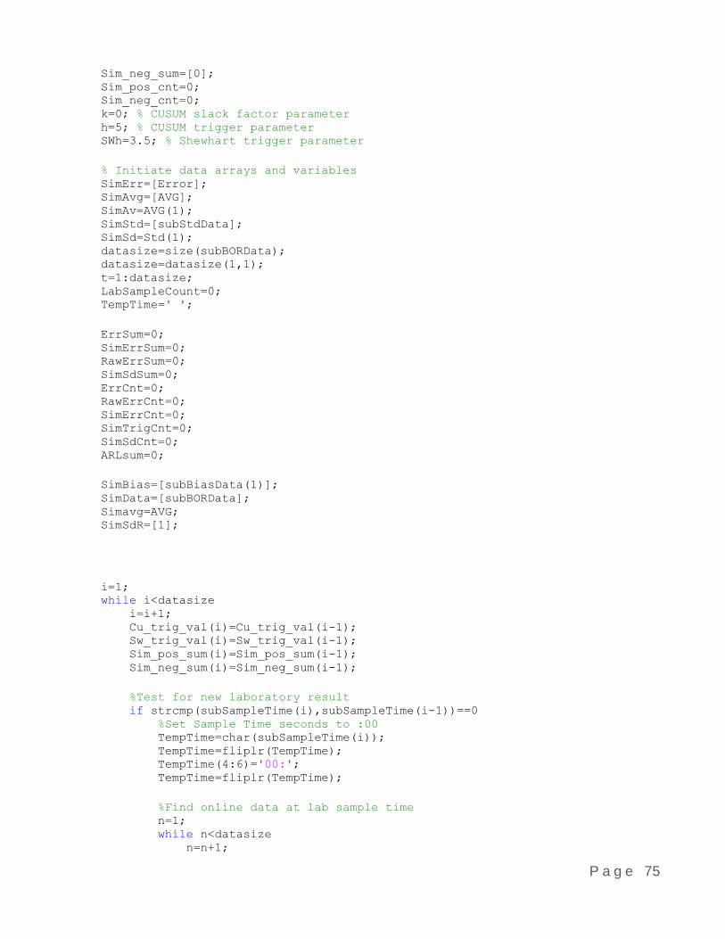
P a g e 75

Sim_neg_sum=[0]; Sim_pos_cnt=0; Sim_neg_cnt=0; k=0; % CUSUM slack factor parameter h=5; % CUSUM trigger parameter SWh=3.5; % Shewhart trigger parameter

% Initiate data arrays and variables SimErr=[Error]; SimAvg=[AVG]; SimAv=AVG(1); SimStd=[subStdData]; SimSd=Std(1); datasize=size(subBORData); datasize=datasize(1,1); t=1:datasize; LabSampleCount=0; TempTime=' ';

ErrSum=0; SimErrSum=0; RawErrSum=0; SimSdSum=0; ErrCnt=0; RawErrCnt=0; SimErrCnt=0; SimTrigCnt=0; SimSdCnt=0; ARLsum=0;

SimBias=[subBiasData(1)]; SimData=[subBORData]; Simavg=AVG; SimSdR=[1];

i=1; while i<datasize i=i+1; Cu_trig_val(i)=Cu_trig_val(i-1); Sw_trig_val(i)=Sw_trig_val(i-1); Sim_pos_sum(i)=Sim_pos_sum(i-1); Sim_neg_sum(i)=Sim_neg_sum(i-1);


%Find online data at lab sample time n=1; while n<datasize n=n+1;

P a g e 76

if strcmp(TempTime,subTimeStamp(n))==1 TestData=[SimData(n-x_val:n+x_val)]; SimAv=mean(TestData); SimSd=std(TestData); SimErr(i)=subLabData(i+2)-SimAv; RawErr=subLabData(i+2)-RawAVG(i); ErrData=subLabData(i+2)-subAvgData(i+2); LabSampleCount=LabSampleCount+1;

% Average error calculations if



abs(SimErr(i))<max_err&&SimSd<sd_hi&&SimSd>sd_lo&&subLabData(i)<lab_hi&&subLabDa

ta(i)>lab_lo&&subLabData(i+2)==subLabData(i+3) RawErrSum=RawErrSum+abs(RawErr); RawErrCnt=RawErrCnt+1; end

%Shewhart and CUSUM calculation if parameters are within limits if

abs(SimErr(i))<max_err&&SimSd<sd_hi&&SimSd>sd_lo&&subLabData(i)<lab_hi&&subLabDa

ta(i)>lab_lo&&subLabData(i+2)==subLabData(i+3) SimSdCnt=SimSdCnt+1; SimSdSum=SimSdSum+SimSd; SimSdAvg=SimSdSum/SimSdCnt; Cu_trig_val(i)=h*SimSdAvg; Sw_trig_val(i)=SWh*SimSdAvg; Sim_pos_sum(i)=max(0,((subLabData(i+2)-(k*SimSd))-

SimAv)+Sim_pos_sum(i-1)); Sim_neg_sum(i)=min(0,((subLabData(i+2)-(k*SimSd))-

SimAv)+Sim_neg_sum(i-1)); SimErrSum=SimErrSum+abs(SimErr(i)); SimErrCnt=SimErrCnt+1; else Sim_pos_sum(i)=Sim_pos_sum(i-1); Sim_neg_sum(i)=Sim_neg_sum(i-1); Cu_trig_val(i)=Cu_trig_val(i-1); Sw_trig_val(i)=Sw_trig_val(i-1); end

%Bias adjustment calculation if SimErr(i-1)>Sw_trig_val(i) Sim_n_adj=SimErr(i); SimTrigCnt=SimTrigCnt+1; ARLsum=ARLsum+1; elseif SimErr(i-1)<((-1)*Sw_trig_val(i)) Sim_n_adj=SimErr(i); SimTrigCnt=SimTrigCnt+1; ARLsum=ARLsum+1; elseif Sim_pos_sum(i-1)>Cu_trig_val(i) Sim_n_adj=Sim_pos_sum(i)/(Sim_pos_cnt+1); SimTrigCnt=SimTrigCnt+1; ARLsum=ARLsum+Sim_pos_cnt;

P a g e 77

elseif Sim_neg_sum(i-1)<((-1)*Cu_trig_val(i)) Sim_n_adj=Sim_neg_sum(i)/(Sim_neg_cnt+1); SimTrigCnt=SimTrigCnt+1; ARLsum=ARLsum+Sim_neg_cnt; else Sim_n_adj=0; Sim_pos_cnt=Sim_pos_cnt+1; Sim_neg_cnt=Sim_neg_cnt+1; end

% Shewhart and CUSUM reset if Sim_pos_sum(i-1)>Cu_trig_val(i)||Sim_neg_sum(i-1)<((-

1)*Cu_trig_val(i-1))||SimErr(i)>Sw_trig_val(i)||SimErr(i-1)<((-

1)*Sw_trig_val(i)) Sim_pos_cnt=0; Sim_neg_cnt=0; Sim_pos_sum(i)=0; Sim_neg_sum(i)=0; SimSdCnt=0; SimSdSum=0; end if Sim_pos_sum(i)==0 Sim_pos_cnt=0; end if Sim_neg_sum(i)==0 Sim_neg_cnt=0; end


%exit while loop break end SimAvg(i)=SimAv; SimStd(i)=SimSd; end else

%Index arrays keeping last value if no change. SimErr(i)=SimErr(i-1); Sim_n_adj=0; SimAvg(i)=SimAvg(i-1); SimStd(i)=SimStd(i-1); end


%Calculate and display average errors

P a g e 78

AvEr=ErrSum/ErrCnt; NewAvEr=SimErrSum/SimErrCnt; RawAvEr=RawErrSum/RawErrCnt; ARL=ARLsum/SimTrigCnt; T=table(AvEr,NewAvEr,RawAvEr,SimTrigCnt,LabSampleCount,ARL)

%Display file and parameters used fprintf('File - %s : Unit - %s.\n',filename,sheet); fprintf('New CUSUM Parameters: k=%d, h=%d\n',k,h);


automatic inferential bias adjustment: optimisation of an

Documents