automating the process for locating no...

AUTOMATING THE PROCESS FOR LOCATING NO-PASSING ZONES

USING GEOREFERENCING DATA

A Ph.D. Dissertation Proposal By

MEHDI AZIMI

Submitted to the Office of Graduate Studies Texas A&M University

in partial fulfillment of the requirement for the degree of DOCTOR OF PHILOSOPHY

Committee Members: Dr. Gene Hawkins (Chair)

Dr. Russell Feagin Dr. Dominique Lord Dr. Yunlong Zhang

July 1, 2011

Major Subject: Civil Engineering

TABLE OF CONTENTS 1. INTRODUCTION ................................................................................................................... 1 2. PROBLEM STATEMENT ..................................................................................................... 1 3. RESEARCH OBJECTIVES .................................................................................................... 1 4. BACKGROUND ..................................................................................................................... 2

4.1. Passing Sight Distance ......................................................................................................... 3 4.1.1. ASHTO Green Book ..................................................................................................... 3 4.1.2. Manual on Uniform Traffic Control Devices ................................................................ 6

4.2. No-Passing Zones ............................................................................................................... 10 4.3. No-Passing Zone Location Methods .................................................................................. 11 4.4. Global Positioning System (GPS) ...................................................................................... 11

4.4.1 WAAS .......................................................................................................................... 12 4.4.2. DGPS ........................................................................................................................... 13 4.4.3. RTK ............................................................................................................................. 13

4.5. GPS Data, Format and Accuracy ....................................................................................... 14 4.6. Geometric Roadway Modeling .......................................................................................... 17

5. RESEARCH TASKS............................................................................................................. 18 5.1. Literature Review ............................................................................................................... 19 5.2. GPS Data Collection and Formatting GPS Data ................................................................ 19 5.3. Geometric Modeling of Highway ...................................................................................... 21 5.4. No-Passing Zone Algorithm Development ........................................................................ 22 5.5. Software Package Development ......................................................................................... 24 5.6. Error Estimation of the Developed Model ......................................................................... 24 5.7. Prototype Model Development and Evaluation ................................................................. 25 5.8. Implementation Guidelines ................................................................................................ 26

6. POTENTIAL BENEFIT OF STUDY ................................................................................... 26 7. SCHEDULE OF ACTIVITIES ............................................................................................. 27 REFERENCES ............................................................................................................................. 28

Deleted:

Deleted:

Deleted:

Deleted:

Automating the Process for Locating No-Passing Zones Using Georeferencing Data Page 1 of 31

1. INTRODUCTION

Two-lane, two-way highways constitute the vast majority of the road system in the U.S. Over 62

percent of the 80,000 centerline highway miles on the TxDOT system are rural two-lane

highways (1). No-passing zones are a significant characteristic of two-lane highways as they

establish locations where passing is prohibited because of restricted sight distance. Locating the

start and end of these zones can be a major challenge. Many methods for locating no-passing

zones are available but there is a need for new methods that can locate no-passing zones in an

efficient, accurate, and safer manner. This research will use GPS data and apply theoretical

approaches to evaluate horizontal and vertical alignment sight distances in order to develop a

method for automating the process for locating no-passing zones.

2. PROBLEM STATEMENT

Locating highway segments that require no-passing zones has been a difficult task because of the

amount of the time necessary to locate the zones and the hazard involved in working on the

highway in the presence of moving traffic. Multiple methods for measuring passing sight

distance and determining no-passing zone are available and range in cost, time, and accuracy.

Although there are several methods for identifying no-passing zones, each one has a set back

because of the time required, accuracy obtained, and related safety issues. Hence, new methods

that will efficiently locate no-passing zones, define the no-passing zones accurately, and do so

safely are needed. GPS has the potential to meet these needs; however, processes for gathering

roadway GPS data, smoothing GPS data, mathematically locating no-passing zones from GPS

data, and implementing the results in the field must be addressed. It is believed that a system

(prototype) enabling work crews to drive on two-lane roadways with GPS units to automatically

determine no-passing zones can be developed by focusing on these issues.

3. RESEARCH OBJECTIVES

The goal of the research is to develop a safe, reliable, fast, and accurate system which automates

the process for locating no-passing zones; and would be applicable to roadways with changes in

both horizontal and vertical alignment. To this end, the research entails the following objectives:


identify the processes necessary to smooth GPS data and geometrically model roadway

surface

create an algorithm for locating no-passing zones from modeled roadway surfaces due to

horizontal and vertical sight obstructions

develop software package and prototype model that can be used by engineers in the field

to establish the location of no-passing zones

provide guidelines for field implementation of the system

4. BACKGROUND

The criteria for locating no-passing zones are contained in the Manual on Uniform Traffic

Control Devices (MUTCD). Location of a no-passing zone for a new highway can be

determined from a set of plans, but the location needs to be confirmed in the field due to

potential differences between the plans and the actual construction. Locating no-passing zones

in the field typically involves surveying activities or two vehicles connected by a rope associated

with the appropriate passing sight distance. Both methods are time consuming, expensive,

subject to error, and can significantly impact other vehicles traveling on the roadway.

Furthermore, these procedures place workers in the presence of moving traffic. In addition to

determining the location of no-passing zones for a new highway, the location need to be

reestablished whenever the speed limit changes, when obstacles are placed that block the sight

distance in the vertical or horizontal plane, and sometimes when the pavement is resurfaced.

Therefore, there is a need for an automated method to locate no-passing zones that is ready for

implementation by transportation agencies. Previous research efforts have addressed some

aspects related to this need (2, 3), but none of them have produced a comprehensive product that

is ready for implementation. This research intends to develop a method for locating no-passing

zones that is based on GPS and would consider both horizontal and vertical alignment

perspectives of the roadway. The development of such an automated system could save time and

cost, avoid human errors, and be safer compared to the current methods of the field

measurements.


4.1. Passing Sight Distance

Sight distance is the length of roadway visible to a driver. The American Association of State

Highway and Transportation Officials (AASHTO) states that the designer should provide

sufficient sight distance for the drivers to control operation of their vehicles before striking

unexpected objects in the traveled way (4). Two-lane highways should also have sufficient sight

distance to provide opportunities for faster drivers to occupy the opposing traffic lane for passing

other vehicles without risk of a crash where gaps in opposing traffic permit. Two-lane rural

highways should generally provide such passing sight distance at frequent intervals and for

substantial portions of their length.

Two types of passing sight distance criteria for two-lane highways are used by highway

agencies: geometric design and marking criteria. Therefore, separate criteria are used in

designing the highways and in marking no-passing zones on the highways. The AASHTO Green

Book and MUTCD both cover the subject of passing sight distance. The contents of these

documents are briefly covered below.

4.1.1. ASHTO Green Book

AASHTO Green Book (4) presents a model for determining the passing sight distance based on

the results of field studies conducted between 1938 and 1958 (5). The model incorporates three

vehicles, and is based on five assumptions:

1. The vehicle being passed travels at a constant speed.

2. The passing vehicle follows the slow vehicle into the passing section.

3. Upon entering the passing section, the passing driver requires a short period of time to

perceive that the opposing lane is clear and to begin accelerating.

4. The passing vehicle travels at an average speed that is 10 mph faster than the vehicle

being passed while occupying the left lane.

5. When the passing vehicle returns to its lane, there is an adequate clearance distance

between the vehicle and an oncoming vehicle in the other lane.

AASHTO passing sight distance is the sum of four distances, as following (Figure 1 gives a

graphical explanation of these elements):

S = d1 + d2 + d3 + d4


where:

S = minimum passing sight distance

d1 = distance traversed during perception and reaction time and during initial acceleration to

the point of encroachment on the left lane;

d2 = distance traveled while the passing vehicles occupies the left lane.

d3 = distance between the passing vehicle at the end of its maneuver and the opposing

vehicle.

d4 = distance traversed by an opposing vehicle for two-thirds of the time the passing vehicle

occupies the left lane, or 2/3 of d2 above.

Figure 1. Elements of Passing Sight Distance for Two-Lane Highways (Exhibit 3-4, AASHTO Green Book)

Table 1 summarizes the results of field observations directed toward quantifying the various

aspects of the passing sight distance.


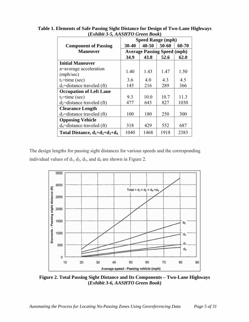
Table 1. Elements of Safe Passing Sight Distance for Design of Two-Lane Highways (Exhibit 3-5, AASHTO Green Book)

Component of Passing Maneuver

Speed Range (mph) 30-40 40-50 50-60 60-70 Average Passing Speed (mph) 34.9 43.8 52.6 62.0

Initial Maneuver a=average acceleration (mph/sec)

1.40 1.43 1.47 1.50

t1=time (sec) 3.6 4.0 4.3 4.5 d1=distance traveled (ft) 145 216 289 366 Occupation of Left Lane t2=time (sec) 9.3 10.0 10.7 11.3 d2=distance traveled (ft) 477 643 827 1030 Clearance Length d3=distance traveled (ft) 100 180 250 300 Opposing Vehicle d4=distance traveled (ft) 318 429 552 687

Total Distance, d1+d2+d3+d4 1040 1468 1918 2383

The design lengths for passing sight distances for various speeds and the corresponding

individual values of d1, d2, d3, and d4 are shown in Figure 2.

Figure 2. Total Passing Sight Distance and Its Components – Two-Lane Highways (Exhibit 3-6, AASHTO Green Book)


AASHTO recommends minimum passing sight distances between 710 and 2680 feet for two-

lane highways for design speeds ranging from 20 to 80 mph (see Table 2). These values are

based on the driver’s eye height being 3.5 feet and the height of the object being 3.5 feet.

Table 2: Passing Sight Distance for Design of Two-Lane Highways

(Exhibit 3-7, AASHTO Green Book)

Design Speed (mph)

Assumed Speeds (mph) Passing Sight Distance

(ft) Passed Vehicle

Passing Vehicle

CalculatedRounded

for Design 20 18 28 706 710 25 22 32 897 900 30 26 36 1088 1090 35 30 40 1279 1280 40 34 44 1470 1470 45 37 47 1625 1625 50 41 51 132 1835 55 44 54 1984 1985 60 47 57 2133 2135 65 50 60 2281 2285 70 54 64 2479 2480 75 56 66 2578 2580 80 58 68 2677 2680

4.1.2. Manual on Uniform Traffic Control Devices

The AASHTO passing sight distance values presented in Table 2 are used for design purposes

only. The Manual on Uniform Traffic Control Devices (MUTCD) developed by the Federal

Highway Administration (6), lays out minimum passing sight distance for placing no-passing

zone pavement markings on completed highways. The MUTCD criteria were first incorporated

in the 1948 MUTCD, identical to those presented in the 1940 AASHO policy on marking no-

passing zones (7), and were used as warrants for no-passing zones (5). The warrants are based

on a compromise between delayed and flying passes. A delayed pass is a maneuver in which the

passing vehicle slows down before making pass. A flying pass is a maneuver in which the

passing vehicle is not delayed by the slower, passed vehicle. Table 3 presents the sight distances

for flying and delayed passes and the minimum sight distances suggested by the 1940 AASHO

policy on marking no-passing zones (7).


Table 3: Sight Distances for Flying and Delayed Passes (7)

V, assumed design speed of the road (mph) 30 40 50 60 70

m, difference in speed between the assumed design speed of the road and the assumed speed of the overtaken vehicle (mph)

10 12.5 15 20 25

V0, assumed speed of an opposing vehicle comes into view just when the passing maneuver is begun (mph)

25 32.5 40 47.5 55

Sight Distances for Flying Passes (ft) 440 550 660 660 660

Sight Distances for Delayed Passes (ft) 510 760 1090 1380 1780

Suggested Minimum Sight Distances (ft) 500 600 800 1000 1200

In the table, V denotes the assumed design speed of the road and is defined as following (7):

“The assumed design speed is considered to be the maximum approximately uniform speed

which probably will be adopted by the faster group of drivers but not, necessarily, by a small

percentage of reckless ones.”

“The design speed of an existing road or section of road may be found by measuring the

speed of travel when the road is not congested, plotting a curve relating speeds to numbers

or percentages of vehicles and choosing a speed from the curve which is greater than the

speed used by almost all drivers. It may also be found by driving the road until a

comfortable maximum uniform speed is found.”

Table 4 lists the MUTCD recommended minimum passing sight distances for various speeds.

Although MUTCD adopted the same minimum passing sight distances from the 1940 AASHO

policy on marking no-passing zones, it defines the symbol V as 85th-percentile/posted/statutory

speed rather than design speed (see Table 4).


Table 4: Minimum Passing Sight Distances for No-Passing Zones Markings (Table 3B-1, MUTCD)

85th Percentile or Posted or Statutory Speed Limit

(mph)

Minimum Passing Sight Distance (ft)

25 450 30 500 35 550 40 600 45 700 50 800 55 900 60 1000 65 1100 70 1200

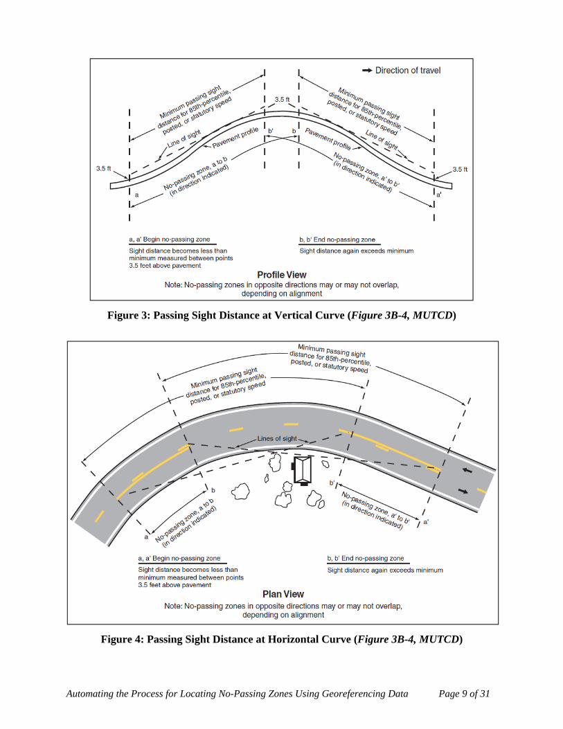
The MUTCD passing sight distance criteria are measured based on 3.5 ft height of driver

eye and 3.5 ft height of object (the 3.5 ft height of object allows the driver to see the top of a

typical passenger car). In other words, it is assumed that the driver's eyes are at a height of 3.5 ft

from the road surface and the opposing vehicle is 3.5 ft tall. The actual passing sight distance is

the length of roadway ahead over which the object would be visible. On a vertical curve, it is the

distance at which an object 3.5 feet above the pavement surface can be seen from a point 3.5 feet

above the pavement (see Figure 3). Similarly, on a horizontal curve, it is the distance measured

along the center line between two points 3.5 feet above the pavement on a line tangent to the

embankment or other obstruction that cuts off the view on the inside of the curve (see Figure 4).


Figure 3: Passing Sight Distance at Vertical Curve (Figure 3B-4, MUTCD)

Figure 4: Passing Sight Distance at Horizontal Curve (Figure 3B-4, MUTCD)


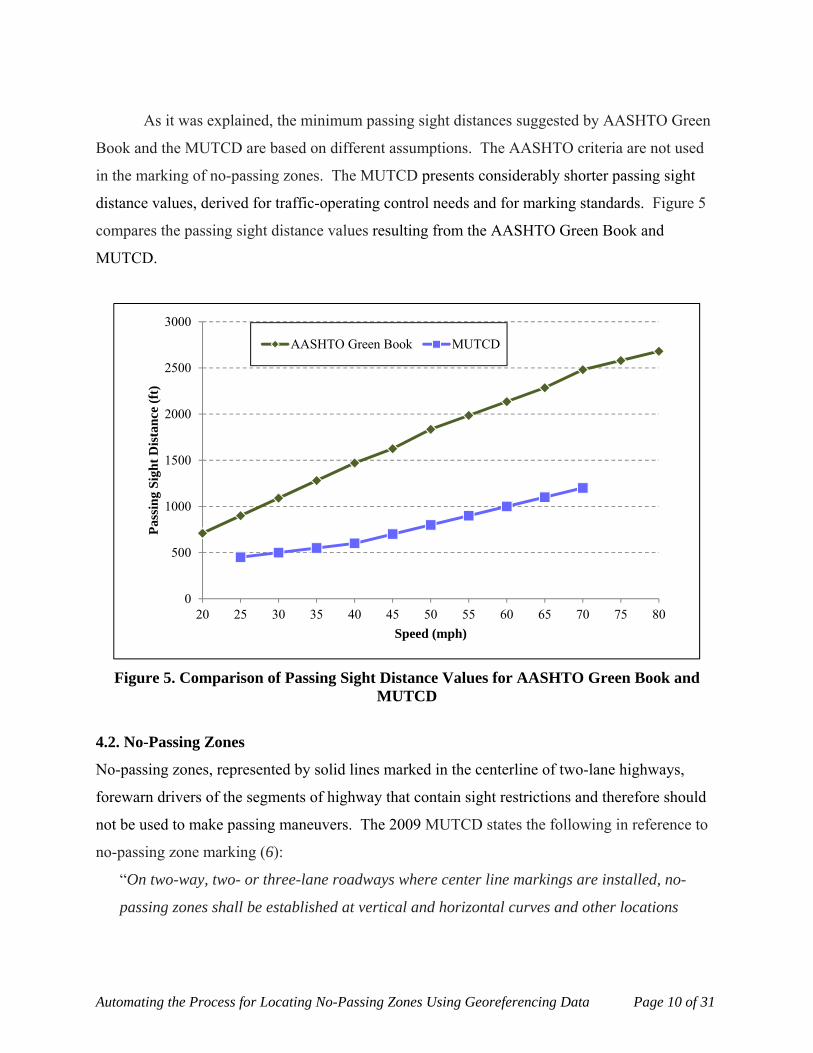
As it was explained, the minimum passing sight distances suggested by AASHTO Green

Book and the MUTCD are based on different assumptions. The AASHTO criteria are not used

in the marking of no-passing zones. The MUTCD presents considerably shorter passing sight

distance values, derived for traffic-operating control needs and for marking standards. Figure 5

compares the passing sight distance values resulting from the AASHTO Green Book and

MUTCD.

Figure 5. Comparison of Passing Sight Distance Values for AASHTO Green Book and MUTCD

4.2. No-Passing Zones

No-passing zones, represented by solid lines marked in the centerline of two-lane highways,

forewarn drivers of the segments of highway that contain sight restrictions and therefore should

not be used to make passing maneuvers. The 2009 MUTCD states the following in reference to

no-passing zone marking (6):

“On two-way, two- or three-lane roadways where center line markings are installed, no-

passing zones shall be established at vertical and horizontal curves and other locations

0

500

1000

1500

2000

2500

3000

20 25 30 35 40 45 50 55 60 65 70 75 80

Pas

sin

g S

igh

t D

ista

nce

(ft

)

Speed (mph)

AASHTO Green Book MUTCD


where an engineering study indicates that passing must be prohibited because of inadequate

sight distances or other special conditions.”

“On roadways with center line markings, no-passing zone markings shall be used at

horizontal or vertical curves where the passing sight distance is less than the minimum

shown in Table 4 for the 85th-percentile speed or the posted or statutory speed limit.”

Neither the AASHTO Green Book nor MUTCD addresses required minimum lengths for passing

zones. But the MUTCD indirectly sets a minimum passing zone length of 400 ft by providing

guidance which was first included in the 1961 edition (5) and is still included in the current

version of the manual (6):

“Where the distance between successive no-passing zones is less than 400 ft, no-passing

zone markings should connect the zones.”

4.3. No-Passing Zone Field Location Methods

There are multiple methods for measuring passing sight distance and determining no-passing

zone in the field including Walking (Two-Person) Method, One-Vehicle Method, Two-Vehicle

Method, Eyeball Method, New Jersey Cone Method, Towed-Target Method, Laser Rangefinder

Method, Optical Rangefinder Method, Distance Measuring Equipment Method, Remote-Control

Vehicle, Speed and Distance Method, and Videolog/Photolog Method (8, 9, 10).

Although there are several methods for identifying no-passing zones, each one has a set

back because of the time required, accuracy obtained, and related safety issues. Additionally,

they rely on judgment in determining the beginning and ending of no-passing zones. However, it

is assumed that by using Global Positioning System (GPS) the location of the no-passing zones

could be obtained more quickly, accurately, and safely.

4.4. Global Positioning System (GPS)

Global Positioning System (GPS) is a satellite-based radio-navigation system that provides

reliable location information where there is an unobstructed line of sight to four or more GPS

satellites. The system provides spatial coordinate triplets of longitude, latitude, and elevation for

each point. GPS is maintained by the United States government and consists of three parts: the

space segment, the control segment, and the user segment. The space segment is composed of


24 to 32 satellites and also includes the boosters required to launch them into orbit. The control

segment is composed of a master and alternate control, and a host of ground antennas and

monitor stations. The user segment is composed of users of the Standard Positioning Service.

There are factors that can degrade the GPS signal and thus affect the accuracy of GPS. The

factors include ionosphere and troposphere delays, signal multipath, receiver clock errors,

orbital errors, number of satellites visible, and satellite geometry/shading. High-end GPS

systems reduce GPS errors and provide more accurate and reliable readings by using a

differential signal broadcasted from either known locations (reference stations) on Earth or other

satellite networks. Reference stations track the satellites and have a true range to each satellite

(the exact number of wave-lengths between itself and the satellite). This information, along with

its known location, is sent to the receiver (see Figure 6). High-end GPS devices are usually

divided into four categories with different accuracy levels: WAAS, DGPS (sub-meter and

decimeter), and RTK (centimeter) systems. It should be noted that many vendors are highly

optimistic on claimed accuracy, and most of those accuracies are based on pass-to-pass accuracy

and not repeatability (12). Repeatability is the ability to return to the exact same location at any

time.

Figure 6. GPS Signal Correction

4.4.1 WAAS

WAAS stands for Wide Area Augmentation System. A WAAS-capable receiver can provide a

position accuracy of better than ten feet 95 percent of the time. WAAS consists of

approximately 25 ground reference stations positioned across the United States that monitor GPS

3. Signal is corrected and broadcast to high‐end receivers.

2. Reference station receives signals.

1. Satellite broadcast GPS signal.

Differential Signal


satellite data. Two master stations, located on either coast, collect data from the reference

stations and create a GPS correction message. The corrected differential message is then

broadcast through one of two geostationary satellites, or satellites with a fixed position over the

equator. The information is compatible with the basic GPS signal structure, which means any

WAAS-enabled GPS receiver can read the signal. For some users in the U.S., the position of the

satellites over the equator makes it difficult to receive the signals when trees or mountains

obstruct the view of the horizon. WAAS signal reception is ideal for open land and marine

applications. WAAS provides extended coverage both inland and offshore compared to the land-

based DGPS system (11).

4.4.2. DGPS

Differential Global Positioning System (DGPS) is an extension of the GPS system that uses land-

based radio beacons to transmit position corrections to GPS receivers. It consists of a network of

towers that receive GPS signals and transmit a corrected signal by beacon transmitters. In order

to get the corrected signal, users must have a differential beacon receiver and beacon antenna in

addition to their GPS. DGPS systems require a differential signal from either a free service or a

commercial service. One of the famous free services is Coast Guard Beacon. OmniStar and

John Deere’s StarFire (SF) systems are in the list of commercial services. Those services need

subscription and the cost of their subscription varies. OmniStar VBS costs $800 per year and

requires only a single channel receiver. OmniStar HP costs $1500 per year and requires a dual

channel receiver. The SF I is a free signal for those who buy the hardware, and the SF II costs

$800/yr. SF II requires a dual channel receiver like OmniStar HP (12).

4.4.3. RTK

Real Time Kinematic (RTK) is not only the most accurate of all GPS systems, but the only

system that can achieve complete repeatability, allowing a user to return to the exact location,

indefinitely. RTK utilizes two receivers: a static ground base station and one or more roving

receivers. The base station receives measurements from satellites and communicates with the

roving receiver(s) through a radio link. The roving receiver processes data in real-time to

produce an accurate position relative to the base station. All of this produces measurements with

an immediate accuracy to within 1 to 2 inches. The total cost of a full RTK system with base


station, receiver, data logger, and software is usually around $40,000 (12). In addition to the

high cost of the system, there are some issues related to applying the RTK systems. For

example, there always needs to be line of sight between the ground station of the RTK and the

roving receiver; and the distance between them should always be within 6 to 10 miles. The

receiver must also simultaneously track five satellites to become initialized, and then continue to

track four satellites to remain initialized. Furthermore, RTK needs a time up to 30 minutes

before it begins initialization (12).

Table 5. Comparison of Different GPS Devices

Basic GPS Devices

High-End GPS Devices

WAAS Sub-meter Decimeter Centimeter

Price Range

< $100 $100 - $500 $500 - $2500 $2500 - $7500 $15,000 - $50,000

Source of Signal

Correction - WAAS

US Coast Guard,

OmniStar VBS, StarFire I, local

differential services

OmniStar HP, StarFire II

(requires dual-channel receiver)

real time kinematic (RTK) systems (require a base station within

6-10 miles)

Accuracy1 10 - 100 feet 3 - 10 feet 1 - 3 feet 3 - 12 inches < 1 - 2 inches

Advantage

lowest cost, small handheld

unit, no additional

equipment or service fees are

required

low cost, good accuracy, small

handheld unit, no additional

equipment or service fees are

required

better accuracy best accuracy without using

RTK

highest accuracy, repeatability2

1. Accuracy in horizontal position 2. Repeatability is the ability to return to the exact same location at any time.

4.5. GPS Data, Format and Accuracy

The true figure of the Earth is spheroid or ellipsoid. Every position on Earth is uniquely defined

by GPS data in the format of longitude λ, latitude φ, and altitude above or below sea level.

Longitude and latitude are angles measured from the earth’s center to a point on the earth’s

surface (Figure 7). The angles are measured in degrees or in grads.


Figure 7. Definition of Longitude and Latitude of a Position on Earth (13)

Young and Miller (14) showed that the spatial error from successive GPS data is highly

correlated. Even though the GPS error is widely published to be in the range of 1 to 5 meters,

the relative accuracy of sequential GPS data is much greater. If successive GPS data points use

the same constellation of satellites, the relative error between the two data points is minimal.

Assuming absolute errors of 2 m and 5 m, respectively, for horizontal and vertical error, the

relative error between successive readings is easily sub-meter in both dimensions. The error

correlation between successive GPS data was estimated between the 0.99- and 0.999-level in the

work performed by Young and Miller (14). They showed that the absolute position error of their

three-dimensional model is reduced as a function of the number of observations. Figure 8 shows

the hypothetical reduction in the absolute position error of the 3D model as a function of the

number of observations, assuming 2-m and 5-m random errors, respectively, for horizontal and

vertical positions.


Figure 8. Hypothetical Reduction in the Absolute Position Error of the 3D Model as a Function of the Number of Observations (Young and Miller, 2005)

Young and Miller believed that the high correlation of GPS data error provides in essence a high

quality estimate of heading in the horizontal plane and grade in the vertical plane. Additional

error reduction arises because successive estimates of slope are highly independent, unlike

position estimates. Figure 9 indicates that the relative shape of the roadway is consistently

captured in the GPS data, despite the differences in absolute elevation. Since the researcher did

not collect the GPS data in the field but used GPS data from previous roadway inventory, the

figures suggest that possibly several different GPS receivers, each with a different bias, were

used to collect the elevation data.

0

0.5

1

1.5

2

2.5

3

3.5

4

4.5

5

1 2 3 4 5 6 7 8 9 10 11 12 13 14 15 16 17 18 19 20

Sta

ndar

d D

evia

tion

of

the

Est

imat

e of

the

Mea

n

Number of Samples

Elevation

Horizontal Position


Figure 9. GPS elevation for a Kansas Highway section, K-177 (Young and Miller, 2005)

4.6. Geometric Roadway Modeling

Kansas Department of Transportation (KDOT) collected spatial data on a highway system using

annual GPS surveys. Ben-Arieh et al. (15) described a methodology for cleaning up this large

amount of data, considering it, and generating an approximation of the highway. Nehate and Rys

(16) developed a model using GPS data for determining the available sight distance on 3D

combined horizontal and vertical alignments. Piecewise parametric equations in the form of

cubic B-splines were used to represent the highway surface and sight obstructions, including

tangents (grades), horizontal curves, and vertical curves. Namala and Rys (17) developed a

model for measuring passing sight distance and identifying no-passing zones. Their model was

based on AASHTO design guidelines for passing sight distances and MUTCD criteria for

marking no-passing zones. However, in practice the MUTCD is the only field guide used for

marking no-passing zones. Furthermore, they used GPS data from previous roadway inventory

logs obtained from data collection vehicles and didn’t test their model in the field for locating the

no-passing zones. Young and Miller (14) addressed many of the errors associated with GPS data

and methods for combining historically logged roadway data from KDOT. Easa et al. (18)

developed an analytical model for creating vertical profiles from field data. The model divided


roadways into segments of tangents, crest curves, and sag curves based on trends in incremental

slopes of field data points. Then the tangents and vertical curve segments were fit by linear

regression and splines, respectively. To identify the vertical profiles of roadways from field

data, Easa (19) developed an algorithm for determining optimum vertical alignments from field

data based on optimization methods. Makanae (20) examined an application of parametric

curves used as spatial curves to highway alignment. The study showed that cubic and quadratic

B-spline curves are suitable for application to highway alignment with a relatively large and

small radius of curvature, respectively.

5. RESEARCH TASKS

This research will develop a method for automating the process for locating no-passing zones by

building upon the theoretical approaches used by others for vertical alignment (3) and

developing new theoretical concepts to address the horizontal alignment concepts. The research

will begin with reviews of traditional methods used to locate no-passing zones and prior research

to develop automated methods. The next activity will be to determine the optimal method for

collecting and formatting GPS data or use existing GPS data provided by highway agencies.

Then the main research activity will be to develop an analytical algorithm to locate no-passing

zones that considers both horizontal and vertical alignments. The vertical alignment sight

distance is expected to be based on whether the pavement surface blocks the sight line between

the observer and target. The horizontal alignment sight distance is expected to be based on a

width of roadway (including the traveled way, shoulders, and roadside) defined by the user to be

free of sight obstructions. Being able to combine the sight distance information for the vertical

and horizontal alignment is another key aspect of this activity. The result of these two main

activities will be a preliminary prototype method that is ready for experimental evaluation. Once

ready, the preliminary prototype will be used to collect data in the field and identify the

recommended locations for no-passing zones. The recommended locations will be compared to

the actual locations. In addition, the accuracy of the actual locations will be evaluated for some

portion of the sample to ensure that the existing no-passing zone markings are properly located.

The results of the evaluation will be used to develop the final prototype and the necessary

material so that the prototype can be fabricated by others. The final prototype expected to


consist of a laptop computer, a software package developed through this project, and a GPS

receiver. The research tasks are explored below.

5.1. Literature Review

The initial step in this study is a thorough literature review on the subject to understand the

previous work and topics associated with the research. This background information will aid the

researcher throughout the entire process. Specific areas of interest for the literature review are:

a) brief history of no-passing zones

b) vertical and horizontal alignment sight distances

c) traditional methods used to locate no-passing zones

d) background on GPS technology

e) previous studies which applied the GPS technology in evaluating sight distances

f) geometric modeling of roadways, and

g) automated location of no-passing zones

5.2. GPS Data Collection and Formatting GPS Data

The purpose of this task is preparing a data collection plan, collecting GPS data, and converting

the data to a usable format for input into the model. First, the researcher will develop a data

collection plan to identify the sample size of the roadway alignments required for the study,

locations of the testing sites, time/date of data collection, etc. Sample size depends on number of

roadway alignments, length of the alignments, and number of horizontal and vertical curves and

other critical points in the alignments. Accuracy of the GPS data is another important parameter

in selecting sample size.

The focus of the current research is on collecting GPS data for locating no-passing zones.

It is clear that for this research, the accuracy in absolute position of the successive GPS data

points is not as important as the accuracy of the relative position. Hence, based on the research

conducted by Young and Miller (13), collecting GPS data from one location in several runs do

not help in improving the accuracy of the data for this study. For example, if multiple GPS runs

of the same roadway are collected within 15 minutes of each other, or even an hour, they should

have similar errors and have relative accuracy when compared to one another. However, it is


better to collect more than one sample run from each roadway since it might happen that some

points of the data are missing due to the positions of the satellites and obstructions.

GPS receivers with different technologies are available today to be used in the data

collection but it is not in the scope of this research to analyze and evaluate each option. Instead

two accessible GPS equipments which have different high-end technologies (WAAS and DGPS)

will be used for the data collection. The Center for Transportation Safety at the Texas

Transportation Institute (TTI) has two types of GPS packages from different manufacturers

which have different capabilities: GeoChron Blue and Trimble® DSM232. The reason for using

two different GPS equipments is comparing the results of the data in Task 8 (Prototype Model

Development and Evaluation) and selecting the most appropriate GPS unit for the prototype

model, in terms of price and accuracy. The GeoChron Blue (see Figure 10) has WAAS feature

and the collection rate capability of this device is one hertz. It means that the GPS data can be

collected and stored at a time interval of one second.

Figure 10. GeoChron Blue - Field-hardened GPS Logger with Bluetooth®

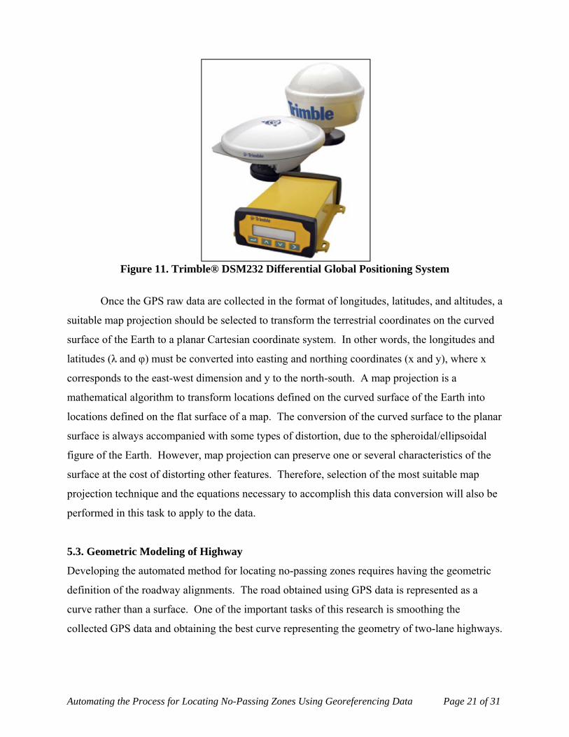
The Trimble® DSM232 system uses commercial satellite correction services provided by

OmniSTAR and provides sub-meter accuracy in real time (see Figure 11). The collection rate

capability of the unit is ten hertz and accuracy of the device is as following (21):

X, Y position (differential/RTK): 0.25m / 0.01m

Height (differential/RTK): 0.5m / 0.02m


Figure 11. Trimble® DSM232 Differential Global Positioning System

Once the GPS raw data are collected in the format of longitudes, latitudes, and altitudes, a

suitable map projection should be selected to transform the terrestrial coordinates on the curved

surface of the Earth to a planar Cartesian coordinate system. In other words, the longitudes and

latitudes (λ and φ) must be converted into easting and northing coordinates (x and y), where x

corresponds to the east-west dimension and y to the north-south. A map projection is a

mathematical algorithm to transform locations defined on the curved surface of the Earth into

locations defined on the flat surface of a map. The conversion of the curved surface to the planar

surface is always accompanied with some types of distortion, due to the spheroidal/ellipsoidal

figure of the Earth. However, map projection can preserve one or several characteristics of the

surface at the cost of distorting other features. Therefore, selection of the most suitable map

projection technique and the equations necessary to accomplish this data conversion will also be

performed in this task to apply to the data.

5.3. Geometric Modeling of Highway

Developing the automated method for locating no-passing zones requires having the geometric

definition of the roadway alignments. The road obtained using GPS data is represented as a

curve rather than a surface. One of the important tasks of this research is smoothing the

collected GPS data and obtaining the best curve representing the geometry of two-lane highways.


In this task, the researcher applies a method to smooth the processed GPS data and then, selects a

mathematical model to represent the geometric definition for roadway alignments.

The accuracy of GPS data, especially when collected from a moving vehicle, can vary

drastically due to the satellite positions; and smooth profiles cannot be taken directly from a

single GPS data collection run. However, multiple data collection runs have unnecessary

repetitions in data. Therefore a suitable method needs to be selected for cleaning data from

repetitions and possible errors. This task has to be performed by using a computer algorithm due

to the large amount of data. The algorithm combines the various data streams together, removes

outliers, and generates correct spatial points. Then a mathematical curve fitting model for

approximation of the highway geometry will be applied. In general, curve fitting models are

used for different purposes such as parameter estimation, functional representation, data

smoothing, or data reduction. Our objective in this part of the research is to perform a curve

fitting process on the set of data points for the purposes of data smoothing and functional

representation. Parametric curves defined with piecewise polynomials such as cubic spline

curves, Bezier cruves, quadratic B-spline curves, and cubic B-spline curves have been used in

the previous studies to obtain geometric definition of highways (15, 20). The researcher will

examine those models to define the best presentation of highways, along with possible new

fitting models (e.g. genetic algorithm). In summary, the mathematical model necessary to

smooth the GPS data and to obtain geometric modeling of highway will be selected in this step

of the research.

5.4. No-Passing Zone Algorithm Development

After geometric modeling of two-lane highways, the main research activity will be to develop a

systematic approach for analyzing smoothed data to locate no-passing zones (no-passing zone

algorithm). Previous research efforts have been done related to this need (2, 3); but either they

have not been comprehensive products ready for implementation or have addressed only the

vertical aspect related to this need. In particular, a recent TAMU master’s thesis addressed using

global positioning system (GPS) to automatically locate no-passing zones for vertical

alignments, but only the vertical alignment issue was addressed and only from a theoretical

perspective.


In two-lane highways, sight distance may be obstructed by horizontal alignments, vertical

alignments, or a combination of both. Being able to combine the sight distance information for

the vertical and horizontal alignments is the key aspect of this activity. In this task, the

researcher will identify the important parameters which must be used in the model to measure

horizontal and vertical sight distances. The parameters include height of driver’s eye, height of

object, lane width, shoulder width, visual clear zone, etc. Then an analytical algorithm will be

developed using projections of the roadway on 2D planes. The input to the algorithm should be

the definition of the roadway produced from the smoothing process and geometric modeling

task. The output of the algorithm should be starting and ending stations of no-passing zones on a

roadway. Considering the MUTCD recommended minimum passing sight distances related to

the posted speed of the highway, a no-passing zone for a segment of the roadway will be

required where the pavement surface elevation is above the needed sight line in vertical curves.

Sight line is defined as a line of sight which is 3.5 feet above the pavement surface on each end.

In horizontal curves, no-passing zone is required if the sight line intersects outer edge of visual

clear zones in either side of the roadway. Visual clear zones are corridors of unobstructed vision

immediately adjacent to the both side of two-lane highways, permitting vehicle drivers to see

approaching vehicles. The algorithm will examine the intersection of sight line and roadway

surface or other obstructions. An iterative process will be used in the algorithm to measure the

horizontal and vertical sight distances. Then the algorithm would compare the resulted sight

distances (horizontal and vertical) and select the lower bound to pinpoint location of no-passing

zones for that specific segment of the roadway. In this research, we define the lower bound as

aggregate overlapping horizontal and vertical sight distances.

According to the MUTCD (6), the passing sight distance on a horizontal curve is the

distance measured along the center line between two points (3.5 feet above the pavement) on a

line tangent to the embankment or other obstruction that cuts off the view on the inside of the

curve (see Figure 4). The data collected with the GPS equipments do not correspond with the

roadway centerline since the vehicle that collects the data travels on one direction of the roadway

and does not go over the centerline. Assuming the vehicle follows a path centered on its lane

and the GPS antenna is mounted on top of the vehicle directly above the center of gravity of the

vehicle, the geometric definition of the roadway obtained in Task 3 represents the centerline of

the traveled lane. Therefore, the no-passing zone algorithm needs to be developed in such a way


that it determines the location of no-passing zones, not only for the traffic in direction of data

collection but for the traffic approaching the opposite direction. No-passing zones for traffic in

opposite directions may overlap or there may be a gap between their ends.

5.5. Software Package Development

The purpose of this task is to develop a software package that implements the algorithms

designed in the previous steps. This package is a user-friendly software that integrates the

programs for GPS conversion, data cleaning, data smoothing, and no-passing zone algorithms.

For coding this software, the main objective is to have an efficient program that has an easy-to-

use Graphical User Interface (GUI). Therefore several computer programming languages will be

examined to find the best one which can code the algorithms easily and also provide a number of

features for GUI applications. After coding the algorithms, it will be converted to an executable

program file that can run independently on any machine (PC or laptop) without needing to install

any special software or program. In this way, the software package can be easily used by both

work crews in the field and traffic engineers in the office.

5.6. Error Estimation of the Developed Model

This task deals with the potential sources of error in all steps of developing model and algorithm.

The current values for minimum passing sight distances in the MUTCD are based on a

compromise between delayed and flying passes (see Figure 12). For example, the sight distances

for flying pass and delayed pass (with the design speed of 70 mph) are 550 and 760 feet,

respectively. It means that there is a range for the passing sight distance rather than an exact

number. However, the suggested minimum sight distances in the manual related to this speed is

600 feet. Therefore, one of the inaccuracies in locating no-passing zones would be due to the

origin of the passing sight distance warrants. Furthermore, other potential error in the developed

model would be because of inaccuracy in the origin of GPS data, type of GPS receivers, number

of data collection runs, and imprecision associated with the smoothing process of the GPS data,

geometric modeling of highway, and developing the no-passing zone algorithm. The researcher

will examine these potential sources of error and address the way he can account for them.


Figure 12. MUTCD Minimum Passing Sight Distances and Corresponding Delayed and Flying Passes

5.7. Prototype Model Development and Evaluation

A preliminary prototype tool instrument will be designed based on the proposed model which

could be used in the field to establish the location of no-passing zones on the two-lane highways.

The prototype expected to consist of a laptop computer, the software package developed through

the project, and a GPS receiver. Other equipments needed to develop the prototype will also be

identified. Furthermore, the data collected with two different GPS receivers (GeoChron Blue

and Trimble® DSM232) will be compared to study the differences in the results of data

collection and no-passing zone location. It will provide the researcher a better idea in selecting

the appropriate GPS receiver.

Once ready, the preliminary prototype will be used to collect data in the field and identify

the recommended locations for no-passing zones. The recommended locations will be compared

to the actual locations. In addition, the accuracy of the actual locations will be verified for some

portion of the sample to ensure that the existing no-passing zone markings are properly located.

This will be done by travelling to the field and checking the available sight distances. The

vehicle can be parked on the shoulder at an adequate distance before the horizontal or vertical

curve. Using a laser or optical rangefinder and a distance measuring instrument (DMI), the

400

600

800

1000

1200

1400

1600

1800

25 30 35 40 45 50 55 60 65 70 75

Pas

sin

g S

igh

t D

ista

nce

(ft

)

Speed (mph)

Delayed Passes

MUTCD

Flying Passes


distance to a vehicle just disappearing over a hill or around a curve will be measured and

compared with the suggested MUTCD minimum passing sight distance. The impact of

measurement errors will be studied through sensitivity analyses. The results of the evaluation

will be used to develop the final prototype and the necessary material so that the prototype can

be fabricated by others.

5.8. Implementation Guidelines

The goal of this research is to develop an efficient and accurate system for automating the

process for locating no-passing zones that would consider both horizontal and vertical alignment

perspectives of the roadway and also be ready for implementation by transportation agencies.

Therefore, it is necessary to establish guidelines and procedures for field implementation by

work crews. The guidelines include a simple description of the prototype, steps for setting up the

system, steps for data collection to obtain the location of no-passing zones, and description of the

results format. Furthermore, some user-defined parameters related to the data collection

procedure (including but not limited to the frequency of GPS reading, antenna height of the GPS

receiver, and vehicle speed) will be described and documented. After the guidelines are

prepared, they will be asked to be reviewed and tested by someone who is unfamiliar with the

system in order to check how well he/she can understand and follow the given guidelines. This

will help to make further improvements in the guidelines if it feels necessary.

6. POTENTIAL BENEFIT OF STUDY

If this study is successful in developing the model and prototype, it overcomes the disadvantages

associated with the current practices and the transportation agencies would be able to more

efficiently and accurately locate the potential no-passing zones and thus determine the striping

patterns on two-lane highways. Implementing this automated technique and development the

prototype has the potential benefits of saving time and cost and eliminating human errors. More

importantly, it will not only provide a safer method by which field crews can determine the

location of two-lane roadway pavement markings, but also eliminate the need to visually inspect

the sight distance of the highway.


7. SCHEDULE OF ACTIVITIES

The following table presents a schedule of activities for the project.

Task Month

1 2 3 4 5 6 7 8 9 10 11 12

1: Literature Review

2: GPS Data Collection and Formatting GPS Data

3: Geometric Modeling of Highway

4. No-Passing Zone Algorithm Development

5: Software Package Development

6: Error Estimation of the Developed Model

7: Prototype Development and Evaluation

8: Implementation Guidelines


REFERENCES

1. Fitzpatrick, K., A. H. Parham, and M. A. Brewer. Treatment for Crashes on Rural Two-Lane

Highways in Texas. Report No. FHWA/TX-02/4048-2, Texas Transportation Institute, The

Texas A&M University System, College Station, Texas, 2002.

2. Leroux, D. Software Tool for Location of No-Passing Zones Using GPS Data. 24th Annual

Esri International User Conference, 2004.

3. Williams, C. L. Field Location and Marking of No-Passing Zones Due To Vertical

Alignments Using the Global Positioning System. MS Thesis, Department of Civil

Engineering, Texas A&M University, College Station, Texas, 2008.

4. A Policy on Geometric Design of Highways and Streets, fourth edition. American

Association of State Highway and Transportation Officials (AASHTO), Washington, D.C.,

2004.

5. Harwood, D. W., D. K. Gilmore, K. R. Richard, J. M. Dunn, and C. Sun. NCHRP Report

605: Passing Sight Distance Criteria. TRB, National Research Council, Washington, D.C.,

2008.

6. Manual on Uniform Traffic Control Devices for Streets and Highways. Federal Highway

Administration, 2009.

7. A Policy on Criteria for Marking and Signing No-Passing Zones on Two and Three Lane

Roads. American Association of State Highway and Officials (AASHO), Washington, D.C.,

1940.

8. Traffic Control Devices Handbook. Institute of Transportation Engineers. Publication No.

IR-112, Washington, D.C., 2001.

9. Brown, R. L., and J. E. Hummer. Procedure for Establishing No-Passing Zones. Final

Report, FHWA/NC/95-007, FHWA and NCDOT, Raleigh, N.C., 1996.

10. Brown, R. L., and J. E. Hummer. Determining the Best Method for Measuring No-Passing

Zones. In Transportation Research Record 1701, Transportation Research Board,

Washington, D.C., pp 61–67, 2000.

11. What is WAAS? http://www8.garmin.com/aboutGPS/waas.html, Tuesday August 10, 2010.

12. High-End DGPS and RTK Systems, USU NASA Space Grant/Land Grant, Geospatial

Extension Program, Periodic Report, October 2005.


http://extnasa.usu.edu/on_target/downloads/Advanced%20GPS--

RTK%20and%20DGPS.PDF, Monday August 9, 2010.

13. Young, S. E., and R. Miller. High-Accuracy Geometric Highway Model Derived from Multi-

Track, Messy GPS Data. Proceedings of the 2005 Mid-Continent Transportation Research

Symposium, Ames, Iowa, August 2005.

14. Kennedy, M., and S. Kopp. Understanding Map Projections. Esri, 1994.

15. Ben-Arieh, D., S. Chang, M. Rys, and G. Zhang. Geometric Modeling of Roadways Using

Global Positioning System Data and B-Spline Approximation. In Journal of Transportation

Engineering, Vol. 130, No. 5, 632-636, 2004.

16. Nehate, G., and Rys, M. 3D Calculation of Stopping-Sight Distance from GPS Data. Journal

of Transportation Engineering, Vol. 132, No. 9, 691-698, 2006.

17. Namala, S.R., and Rys, M. Automated Calculation of Passing Sight Distance Using Global

Positioning System Data. Kansas State University, Manhattan, Kansas and Kansas

Department of Transportation, Topeka, Kansas, Report No. K-TRAN: KSU-03-02,

2006.Easa, S.M., Hassan, Y., and Karim, Z.A. Establishing Roadway Vertical Alignment

Using Profile Field Data. ITE Journal on the Web, August, pp. 81-86, 1998.

18. Easa, S.M. Optimum Vertical Curves for Roadway Profiles. In Journal of Surveying

Engineering, pp. 147-157, August 1999.

19. Makanae, K. An Application of Parametric Curves to Highway Alignment. In Journal of

Civil Engineering Information Processing System. Vol. 8, pp. 231-238, 1999.

20. RTK DGPS Receivers, Hydro International Product Survey, October 2007,

http://www.hydro-international.com/files/productsurvey_v_pdfdocument_18.pdf, Tuesday

August 10, 2010.

automating the process for locating no...

Documents