Automation & Robotics Research Institute (ARRI)The University of Texas at Arlington

F.L. LewisMoncrief-O’Donnell Endowed Chair

Head, Controls & Sensors Group

Talk available online at http://ARRI.uta.edu/acs

ADP for Feedback Control

Supported by :NSF - PAUL WERBOSARO – JIM OVERHOLT

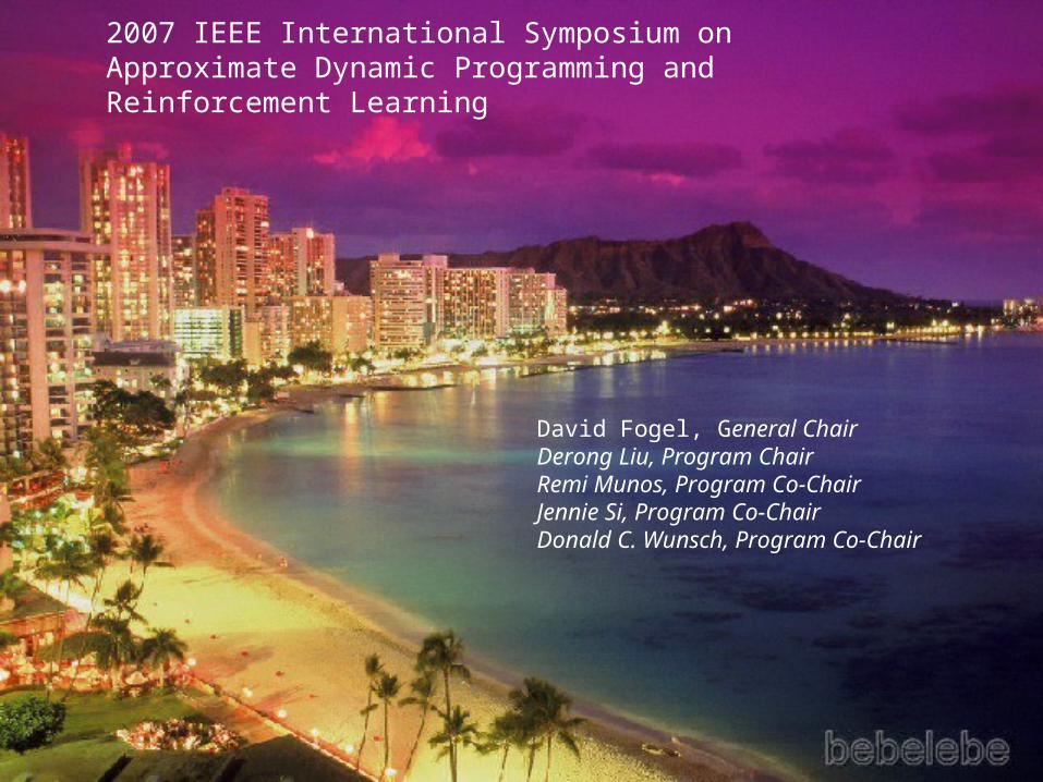
2007 IEEE International Symposium on Approximate Dynamic Programming and Reinforcement Learning

David Fogel, General Chair Derong Liu, Program Chair Remi Munos, Program Co-ChairJennie Si, Program Co-ChairDonald C. Wunsch, Program Co-Chair

Relevance- Machine Feedback Control

qd

qr1qr2

AzEl

barrel flexiblemodes qf

compliant coupling

moving tank platform

turret with backlashand compliant drive train

terrain andvehicle vibrationdisturbances d(t)

Barrel tipposition

qd

qr1qr2

AzEl

barrel flexiblemodes qf

compliant coupling

moving tank platform

turret with backlashand compliant drive train

terrain andvehicle vibrationdisturbances d(t)

Barrel tipposition

Vehicle mass m

ParallelDamper

mc

activedamping

uc

(if used)

kc cc

vibratory modesqf(t)

forward speedy(t)

vertical motionz(t)

surface roughness(t)

k c

w(t)

Series Damper+

suspension+

wheel

Single-Wheel/Terrain System with Nonlinearities

High-Speed Precision Motion Control with unmodeled dynamics, vibration suppression, disturbance rejection, friction compensation, deadzone/backlash control

VehicleSuspension

IndustrialMachines

Military LandSystems

Aerospace

Automation & Robotics Research Institute (ARRI)

Input Membership Fns. Output Membership Fns.

Fuzzy Logic Rule Base

NN

Input

NN

Output

Fuzzy Associative Memory (FAM) Neural Network (NN)

INTELLIGENT CONTROL TOOLS

Input x Output u

Input x Output u

Both FAM and NN define a function u= f(x) from inputs to outputs

FAM and NN can both be used for: 1. Classification and Decision-Making 2. Control

(Includes Adaptive Control)

NN Includes Adaptive Control (Adaptive control is a 1-layer NN)

Neural Network Properties

Learning

Recall

Function approximation

Generalization

Classification

Association

Pattern recognition

Clustering

Robustness to single node failure

Repair and reconfiguration

Nervous system cell. http://www.sirinet.net/~jgjohnso/index.html

Two-layer feedforward static neural network (NN)

(.)

(.)

(.)

(.)

x1

x2

y1

y2

VT WT

inputs

hidden layer

outputs

xn ym

1

2

3

L

(.)

(.)

(.)

Summation eqs Matrix eqs

)( xVWy TT

K

ki

n

jkjkjiki wvxvwy

10

10

Have the universal approximation propertyOvercome Barron’s fundamental accuracy limitation of 1-layer NN

qd

Robot System[I]

Robust ControlTerm

q

v(t)

e

PD Tracking Loop

rKv

Neural Network Robot Controller

^

qd

f(x)

Nonlinear Inner Loop

..

Feedforward Loop

Universal Approximation Property

Problem- Nonlinear in the NN weights sothat standard proof techniques do not work

Feedback linearization

Easy to implement with a few more lines of codeLearning feature allows for on-line updates to NN memory as dynamics changeHandles unmodelled dynamics, disturbances, actuator problems such as frictionNN universal basis property means no regression matrix is neededNonlinear controller allows faster & more precise motion

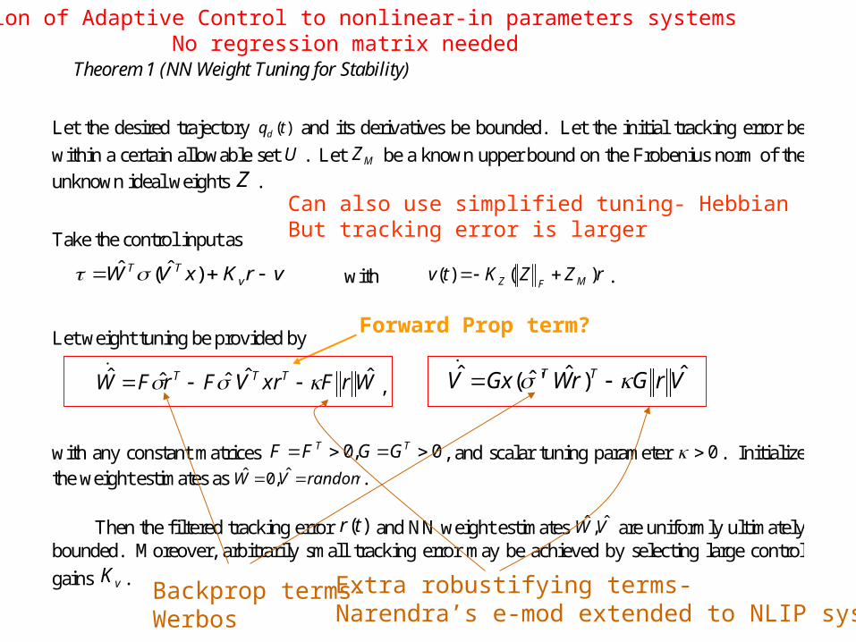
Theorem 1 (NN Weight Tuning for Stability)

Let the desired trajectory )(tqd and its derivatives be bounded. Let the initial tracking error be

within a certain allowable set U . Let MZ be a known upper bound on the Frobenius norm of the

unknown ideal weights Z .

Take the control input as

vrKxVW vTT )ˆ(ˆ with rZZKtv MFZ )()( .

Let weight tuning be provided by

WrFxrVFrFW TTT ˆˆ'ˆˆˆ , VrGrWGxV TT ˆ)ˆ'ˆ(ˆ

with any constant matrices 0,0 TT GGFF , and scalar tuning parameter 0 . Initialize the weight estimates as randomVW ˆ,0ˆ .

Then the filtered tracking error )(tr and NN weight estimates VW ˆ,ˆ are uniformly ultimately bounded. Moreover, arbitrarily small tracking error may be achieved by selecting large control

gains vK . Backprop terms-

Werbos

Extra robustifying terms- Narendra’s e-mod extended to NLIP systems

Forward Prop term?

Can also use simplified tuning- HebbianBut tracking error is larger

Extension of Adaptive Control to nonlinear-in parameters systems No regression matrix needed

Force Control

Flexible pointing systems

Vehicle active suspension

SBIR ContractsWon 1996 SBA Tibbets Award4 US Patents NSF Tech Transfer to industry

More complex Systems?

[I]

Robust ControlTerm vi(t)

Tracking Loop

rKr

Nonlinear FB Linearization Loop

F1(x)^ qr = qr

qr.e

ee = .

qd =qd

qd.

..qd

RobotSystem

1/KB1i

F2(x)^

K

id

NN#1

NN#2

Backstepping Loop

ue

[I]

Robust ControlTerm vi(t)

Tracking Loop

rKrKr

Nonlinear FB Linearization Loop

F1(x)F1(x)^

Neural network backstepping controller for Flexible-Joint robot arm

qr = qr

qr.qr =qr = qr

qr.qr

qr.e

ee = .e = .

qd =qd

qd.qd =qd =qd

qd.qd

qd.

..qd

..qd

RobotSystem

1/KB1i

F2(x)F2(x)^

KK

id

NN#1

NN#2

Backstepping Loop

ue

Backstepping

Advantages over traditional Backstepping- no regression functions needed

Add an extra feedback loopTwo NN neededUse passivity to show stability

Flexible & Vibratory Systems

MechanicalSystem

Kv[

v

reqd

Estimateof NonlinearFunction

w

--

D(u)u

NN DeadzonePrecompensator

wNN

I

II

()fx

q

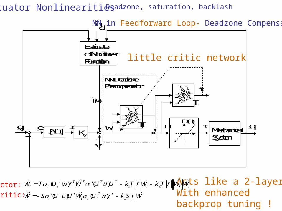
dq NN in Feedforward Loop- Deadzone Compensation

Acts like a 2-layer NNWith enhanced backprop tuning !

little critic network

Actuator Nonlinearities - Deadzone, saturation, backlash

iiiTTTTT

iii WWrTkWrTkUuUWrwUTW ˆˆˆ)('ˆ)(ˆ21

WrSkrwUWUuUSW TTiii

TT ˆ)(ˆ)('ˆ1

Actor:

Critic:

~x 1

( , )h x xo 1 2

( , )h x xc 1 2

ROBOT

Kv

[vc

kD

KvkpM-1(.)

qx

x

1

2

ee

e

qq

qdd

d

x1

x2

z2

1x)(t)(ˆ tr

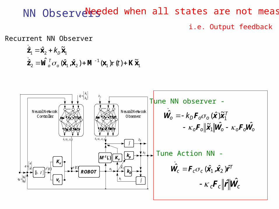
Neural Network Observer

Neural Network Controller

1~x

111

212

121

~)()()ˆ,ˆ(ˆˆ

~ˆˆ

xKxMxxWz

xxz

t

k

oTo

D

NN Observers Needed when all states are not measured

i.e. Output feedback

TooDo k 1

~)ˆ(ˆ xxFW

oooooo WFWxF ˆˆ~1

Tccc rxxFW ˆ)ˆ,ˆ(ˆ

21

ccc WrF ˆˆ

Tune NN observer -

Tune Action NN -

Recurrent NN Observer

Separable Gaussian activation functions for RBF NN

Separable triangular activation functions for CMAC NN

Fuzzy Logic System = NN with VECTOR thresholds

Also Use CMAC NN, Fuzzy Logic systems

Tune first layer weights, e.g.Centroids and spreads-Activation fns move around

Dynamic Focusing of Awareness

Effect of change of membership function spread "a"

Effect of change of membership function elasticities "c"

2cB )b,a,z()c,b,a,z(

2

22

2

1

c

)bz(a

))bz(a(cos)c,b,a,z(

Elastic Fuzzy Logic- c.f. P. Werbos

Weights importance of factors in the rules

ControlledPlantKv[ I]

r(t)

-

Input MembershipFunctions

Fuzzy Rule Base

Output MembershipFunctions

xd(t)

e(t)

-

-

)x,x(g d

x(t)

)x,x(grK)t(u dv raKkrWAKa aa

Ta

rbKkrWBKb bbT

b

rWKkr)cCbBaAˆ(KW WWT

W rcKkrWCKc ccT

c

Elastic Fuzzy Logic Control

Control Tune Membership Functions

Tune Control Rep. Values

Better Performance

Start with 5x5 uniform grid of MFS

Builds its own basis set-Dynamic Focusing of Awareness

After tuning-

Cell Homeostasis The individual cell is a complex feedback control system. It pumps ions across the cell membrane to maintain homeostatis, and has only limited energy to do so.

Cellular Metabolism

Permeability control of the cell membrane

http://www.accessexcellence.org/RC/VL/GG/index.html

Optimality in Biological Systems

Optimality in Control Systems DesignR. Kalman 1960

Rocket Orbit Injection

http://microsat.sm.bmstu.ru/e-library/Launch/Dnepr_GEO.pdf

Fmmm

F

r

wvv

m

F

rr

vw

wr

cos

sin2

2

Objectives Get to orbit in minimum time Use minimum fuel

Dynamics

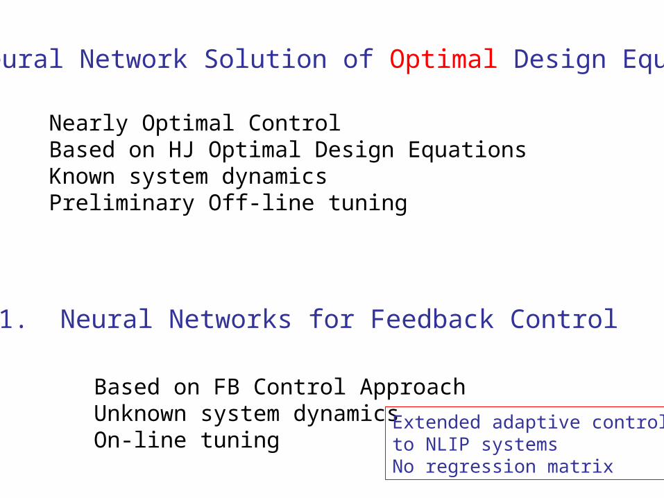
2. Neural Network Solution of Optimal Design Equations

Nearly Optimal ControlBased on HJ Optimal Design EquationsKnown system dynamicsPreliminary Off-line tuning

1. Neural Networks for Feedback Control

Based on FB Control ApproachUnknown system dynamicsOn-line tuning

Extended adaptive control to NLIP systemsNo regression matrix

2 2Tz h h u

2

0

2

0

2

0

2

0

2

)(

)(

)(

)(

dttd

dtuhh

dttd

dttz T

System

),(

)()()(

uxz

xy

dxkuxgxfx

)(ylu

d

u

z

y control

Performance output

Measuredoutput

disturbance

where

Find control u(t) so that

For all L2 disturbancesAnd a prescribed gain

L2 Gain Problem

H-Infinity Control Using Neural Networks

Zero-Sum differential Nash game

Murad Abu Khalaf

Cannot solve HJI !!

CT Policy Iteration for H-Infinity Control

Consistency equationFor Value Function

Successive Solution- Algorithm 1:Let be prescribed and fixed.

0u a stabilizing control with region of asymptotic stability 0

1. Outer loop- update controlInitial disturbance 00 d

2. Inner loop- update disturbanceSolve Value Equation

0)()(2)( 2

0

iTi

u

TTj

Tj

i

dddhhkdgufx

V j

Inner loop update disturbance

x

Vxkd

ji

Ti

)(2

12

1

go to 2.Iterate i until convergence to jVd , with RAS j

Outer loop update control action

x

Vxgu

jTj )(2

11

Go to 1.Iterate j until convergence to

Vu , , with RAS

Murad Abu Khalaf

)()()(

)()( i

LT

Li

L

TL

iL WxW

x

L

x

V

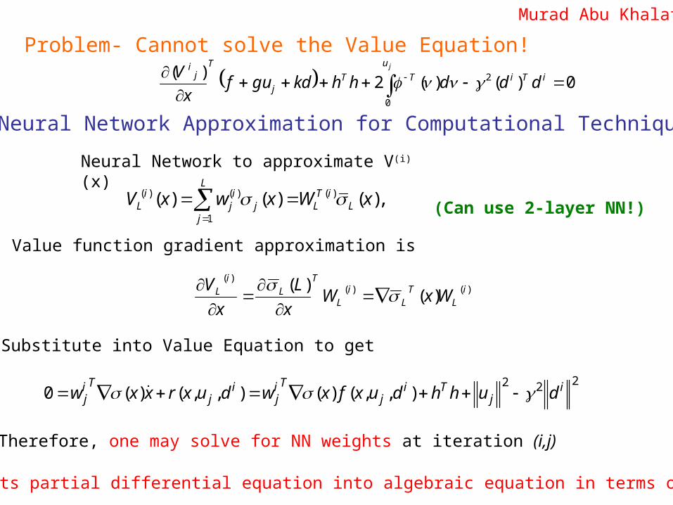
Value function gradient approximation is

Substitute into Value Equation to get

Therefore, one may solve for NN weights at iteration (i,j)

Neural Network Approximation for Computational Technique

222),,()(),,()(0 i

jTi

jTi

ji

jTi

j duhhduxfxwduxrxxw

Neural Network to approximate V(i)(x)

( ) ( ) ( )

1

( ) ( ) ( ),L

i i T iL j j L L

j

V x w x W x

Problem- Cannot solve the Value Equation!

Murad Abu Khalaf

VFA converts partial differential equation into algebraic equation in terms of NN weights

0)()(2)( 2

0

iTi

u

TTj

Tj

i

dddhhkdgufx

V j

(Can use 2-layer NN!)

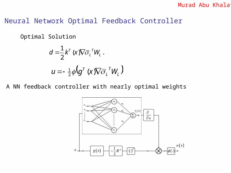
Neural Network Optimal Feedback Controller

1( ) .

2T T

L Ld k x W

Optimal Solution

LT

LT Wxgu )(2

1

A NN feedback controller with nearly optimal weights

Murad Abu Khalaf

Optimal cost

xuxgxf

x

txVL

t

txVT

tu

** ,min

,

Optimal control

x

txVxgRxu T

*

1* ,

2

1

This yields the time-varying Hamilton-Jacobi-Bellman (HJB) equation

0

,,

4

1,, *1

***

x

txVxgRxg

x

txVxQxf

x

txV

t

txV T

T

Fixed-Final-Time HJB Optimal Control

Finite Horizon Control Cheng Tao

Note that txt

x

x

x

txVL

TLL

TLL wσw

σ

,

where is the Jacobian xLσ xxL σ

xtt

txVL

TL

L σw

,

HJB Solution by NN Value Function Approximation Cheng Tao

Approximating in the HJB equation gives an ODE in the NN weights txV ,

xexQ

txxgRxgxt

xfxtxt

L

LTL

TL

TL

LTLL

TL

wσσw

σwσw

1

4

1

Solve by least-squares – simply integrate backwards to find NN weights

)(2

1 1* twxgRxu LTL

T Control is

Time-varying weights

Policy iteration not needed!

Irwin Sandberg

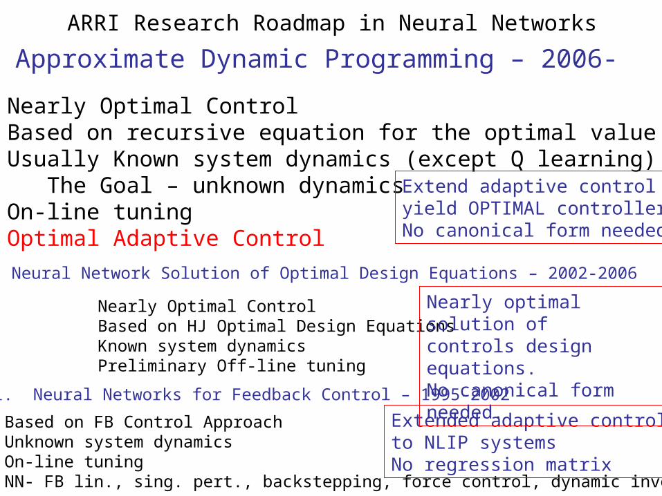
2. Neural Network Solution of Optimal Design Equations – 2002-2006

Nearly Optimal ControlBased on HJ Optimal Design EquationsKnown system dynamicsPreliminary Off-line tuning

1. Neural Networks for Feedback Control – 1995-2002

Based on FB Control ApproachUnknown system dynamicsOn-line tuningNN- FB lin., sing. pert., backstepping, force control, dynamic inversion, etc.

3. Approximate Dynamic Programming – 2006-

Nearly Optimal ControlBased on recursive equation for the optimal valueUsually Known system dynamics (except Q learning) The Goal – unknown dynamicsOn-line tuningOptimal Adaptive Control

ARRI Research Roadmap in Neural Networks

Extended adaptive control to NLIP systemsNo regression matrix

Nearly optimal solution ofcontrols design equations.No canonical form needed.

Extend adaptive control toyield OPTIMAL controllers.No canonical form needed.

Four ADP Methods proposed by Werbos

Heuristic dynamic programming

Dual heuristic programming

AD Heuristic dynamic programming

AD Dual heuristic programming

(Watkins Q Learning)

Critic NN to approximate:

Value

Gradient x

V

)( kxV Q function ),( kk uxQ

Gradientsu

Q

x

Q

,

Action NN to approximate the Control

Bertsekas- Neurodynamic Programming

Barto & Bradtke- Q-learning proof (Imposed a settling time)

ki

iiki

kh uxrxV ),()(

)())(,()( 1 khkkkh xVxhxrxV

))())(,((min)( 1*

khkkh

k xVxhxrxV

Hamiltonian

))(),((min)( 1**

kkku

k xVuxrxVk

))(),((minarg)(* 1*

kkku

k xVuxrxhk

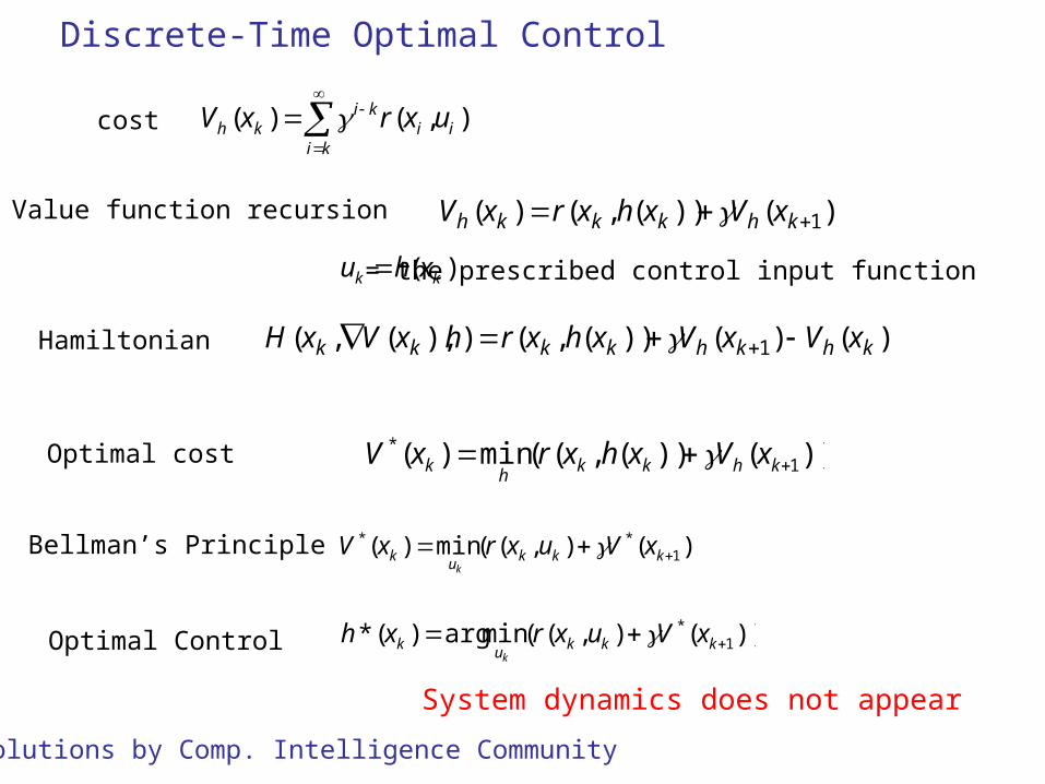
Discrete-Time Optimal Control

cost

Value function recursion

)()())(,()),(,( 1 khkhkkkk xVxVxhxrhxVxH

Optimal cost

Bellman’s Principle

Optimal Control

System dynamics does not appear

)( kk xhu = the prescribed control input function

Solutions by Comp. Intelligence Community

1 ( ) ( )k k k kx f x g x u

1( ) min ( )

min ( ) ( )

k

k

T Tk k k k k ku

T Tk k k k k k ku

V x x Qx u Ru V x

x Qx u Ru V f x g x u

1 1

1

( )1( ) ( )

2T k

k kk

dV xu x R g x

dx

00

( ) k k k kk

V x x Qx u Ru

System

DT HJB equation

Difficult to solve

Few practical solutions by Control Systems Community

Use System Dynamics

Greedy Value Fn. Update- Approximate Dynamic Programming ADP Method 1 - Heuristic Dynamic Programming (HDP)

Paul Werbos

)())(,()( 111 kjkjkkj xVxhxrxV

Policy Iteration

APBBPBIL

RLLQPBLAPBLA

jT

jT

j

jTjjjj

Tj

1

11

)(

)()(

For LQRUnderlying RE Hewer 1971

Initial stabilizing control is NOT needed

Initial stabilizing control is needed

))(),((minarg)( 111 kjkku

kj xVuxrxhk

Lyapunov eq.

Simple recursion

)())(,()( 11 kjkjkkj xVxhxrxV

))(),((minarg)( 111 kjkku

kj xVuxrxhk

ADP Greedy Cost Update

APBBPBIL

RLLQBLAPBLAP

jT

jT

j

jTjjj

Tjj

1

1

)(

)()(

For LQRUnderlying RE Lancaster & Rodman

proved convergence

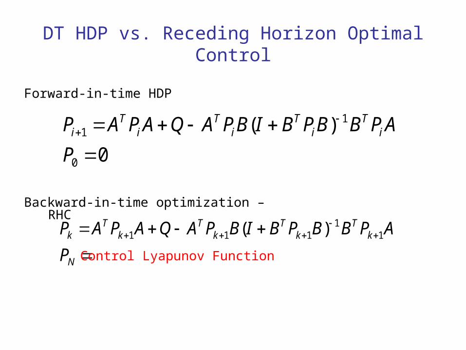
DT HDP vs. Receding Horizon Optimal Control

0

)(

0

11

P

APBBPBIBPAQAPAP iT

iT

iT

iT

i

N

kT

kT

kT

kT

k

P

APBBPBIBPAQAPAP 11

111 )(

Forward-in-time HDP

Backward-in-time optimization – RHC

Control Lyapunov Function

Q Learning

)(),(),( 1 khkkkkh xVuxruxQ policy h(.) used after time k

uk arbitrary

)())(,( khkkh xVxhxQ

Define Q function

Note

))(,(),(),( 11 kkhkkkkh xhxQuxruxQ Recursion for Q

)),((min)( **kk

uk uxQxV

k

Simple expression of Bellman’s principle

)),((minarg)(* *kk

uk uxQxh

k

- Action Dependent ADP

Q Learning does not need to know f(xk) or g(xk)

)(),(),( 1 khkkkkh xVuxruxQ

)()( kkT

kkkTkk

Tk BuAxPBuAxRuuQxx

For LQR PxxxWxV TT )()(

k

k

uuux

xuxxT

k

k

k

kT

k

k

k

kTT

TTT

k

k

u

x

HH

HH

u

x

u

xH

u

x

u

x

PBBRPAB

PBAPAAQu

x

Q is quadratic in x and u

Control update is found by ][2])([20 kuukuxkT

kT

k

uHxHuPBBRPAxBu

Q

sokjkuxuuk

TTk xLxHHPAxBPBBRu 1

11)(

Control found only from Q functionA and B not needed

V is quadratic in x

),(),(),( 1111 kjkjkkkkj xLxQuxruxQ

Q Policy Iteration

)),((minarg)( 11 kkju

kj uxQxhk

Control policy update

),(),(),( 111 kjkkjkkkTj xLxrxLxuxW

kjkuxuuk xLxHHu 11

Model-free policy iteration

Bradtke, Ydstie, Barto

Greedy Q Fn. Update - Approximate Dynamic ProgrammingADP Method 3. Q Learning Action-Dependent Heuristic Dynamic Programming (ADHDP)

Paul WerbosModel-free ADP

))(,(),(),( 111 kjkjkkkkj xhxQuxruxQ

Greedy Q Update

1111 target),(),(),( jkjkTjkjkkk

Tj xLxWxLxruxW

Update weights by RLS or backprop.

Stable initial control needed

Direct OPTIMAL ADAPTIVE CONTROL

Q learning actually solves the Riccati Equation WITHOUT knowing the plant dynamics

Model-free ADP

Works for Nonlinear Systems

Proofs?Robustness?Comparison with adaptive control methods?

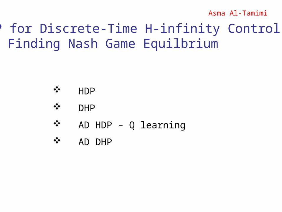
Asma Al-Tamimi

ADP for Discrete-Time H-infinity ControlFinding Nash Game Equilbrium

HDP

DHP

AD HDP – Q learning

AD DHP

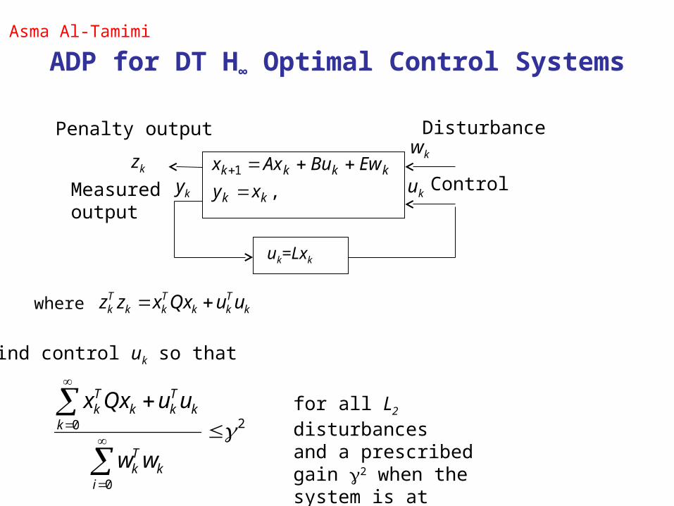
ADP for DT H∞ Optimal Control Systems

,1

kk

kkkk

xy

EwBuAxx

2

0

0

ik

Tk

kk

Tkk

Tk

ww

uuQxx

wk

ukykControl

Penalty output

Measuredoutput

Disturbance

Find control uk so that

for all L2 disturbancesand a prescribed gain 2 when the system is at rest, x0=0.

Asma Al-Tamimi

kTkk

Tkk

Tk uuQxxzz

zk

where

uk=Lxk

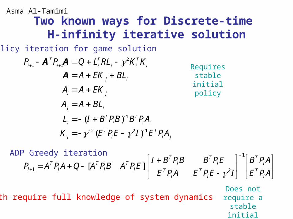
Two known ways for Discrete-time H-infinity iterative solution

ji

T

i

T

j

ii

T

i

T

i

ij

ji

ij

i

T

ii

T

ii

T

i

APEIEPEK

APBBPBIL

BLAA

EKAA

BLEKA

KKRLLQPP

122

1

2

11

)(

)(

Α

ΑΑ

APE

APB

IEPEAPE

EPBBPBIEPABPAQAPAP

iT

iT

iT

iT

iT

iT

iT

iT

iT

i

1

21 ][

Requires stable initial policy

Does not require a stable

initial policy

Policy iteration for game solution

ADP Greedy iteration

Asma Al-Tamimi

Both require full knowledge of system dynamics

DT GameHeuristic Dynamic Programming:

Forward-in-time Formulation• An Approximate Dynamic Programming Scheme (ADP) where one has the

following incremental optimization

which is equivalently written as

)(maxmin)( 12

1 kikTkk

Tkk

Tk

wuki xVwwuuQxxxV

kk

)()()()()()( 12

1 kikikTikik

Tik

Tkki xVxwxwxuxuQxxxV

Asma Al-Tamimi

),)((

))((12

112

APBAPEIEPEEPB

BPEIEPEEPBBPBIL

iT

iT

iT

iT

iT

iT

iT

iT

i

).)((

))((1

112

APEAPBBPBIBPE

EPBBPBIBPEIEPEK

iT

iT

iT

iT

iT

iT

iT

iT

i

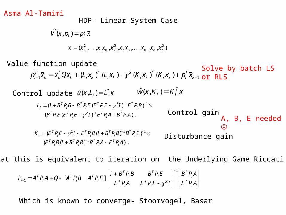
xppxV Tii ),(ˆ

),,,,,,,( 2132

221

21 nnnn xxxxxxxxxx

12

1 )()()()( kTiki

Tkiki

Tkik

Tkk

Ti xpxKxKxLxLQxxxp

HDP- Linear System Case

Value function update

Control update

Control gain

Disturbance gain

Showed that this is equivalent to iteration on the Underlying Game Riccati equation

APE

APB

IEPEAPE

EPBBPBIEPABPAQAPAP

iT

iT

iT

iT

iT

iT

iT

iT

iT

i

1

21 ][

Which is known to converge- Stoorvogel, Basar

Solve by batch LS or RLS

xLLxu Tii ),(ˆ xKKxw T

ii ),(ˆ

A, B, E needed

Asma Al-Tamimi

Q-Learning for DT H-infinity Control:Action Dependent Heuristic Dynamic

Programming

• Dynamic Programming: Backward-in-time

• Adaptive Dynamic Programming: Forward-in-time

)},,(maxminarg{)(

))((),,(

,

12

kkkwu

kk

kkTkk

Tkk

Tkkkk

wuxQwu

xVwwuuRxxwuxQ

kk

)(

)(

),,(maxmin),,(

2

12

1112

111

kkkikTkk

Tkk

Tk

kikTkk

Tkk

Tk

kkkiwu

kTkk

Tkk

Tkkkki

EwBuAxVwwuuRxx

xVwwuuRxx

wuxQwwuuRxxwuxQkk

Asma Al-Tamimi

( ) , ( )i k i k i k i ku x L x w x K x

( ) Tk k kV x x Px

1( , , ) ( , , ) ( )k k k k k k k

TT T T T T Tk k k k k k

Q x u w r x u w V x

x u w H x u w

TTk

Tk

Tki

Tk

Tk

Tkk

Tkk

Tkk

Tk

TTk

Tk

Tki

Tk

Tk

Tk wuxHwuxwwuuRxxwuxHwux ][][][][ 111111

21

wwwuwx

uwuuux

xwxuxx

HHH

HHH

HHH

( ) , ( )i k i k i k i ku x L x w x K x

1 1 1

1 1 1

( ) ( ),

( ) ( ).

i i i i i i i ii uu uw ww wu uw ww wx ux

i i i i i i i ii ww wu uu uw wu uu ux wx

L H H H H H H H H

K H H H H H H H H

))(ˆ),(ˆ,(

)(ˆ)(ˆ)(ˆ)(ˆ))(ˆ),(ˆ,(

111

21

kikiki

kiT

kikiT

kikTkkikiki

xwxuxQ

xwxwxuxuRxxxwxuxQ

Linear Quadratic case- V and Q are quadratic

Q function update

Control Action and Disturbance updates

A, B, E NOT needed

Asma Al-Tamimi

Q learning for H-infinity Control

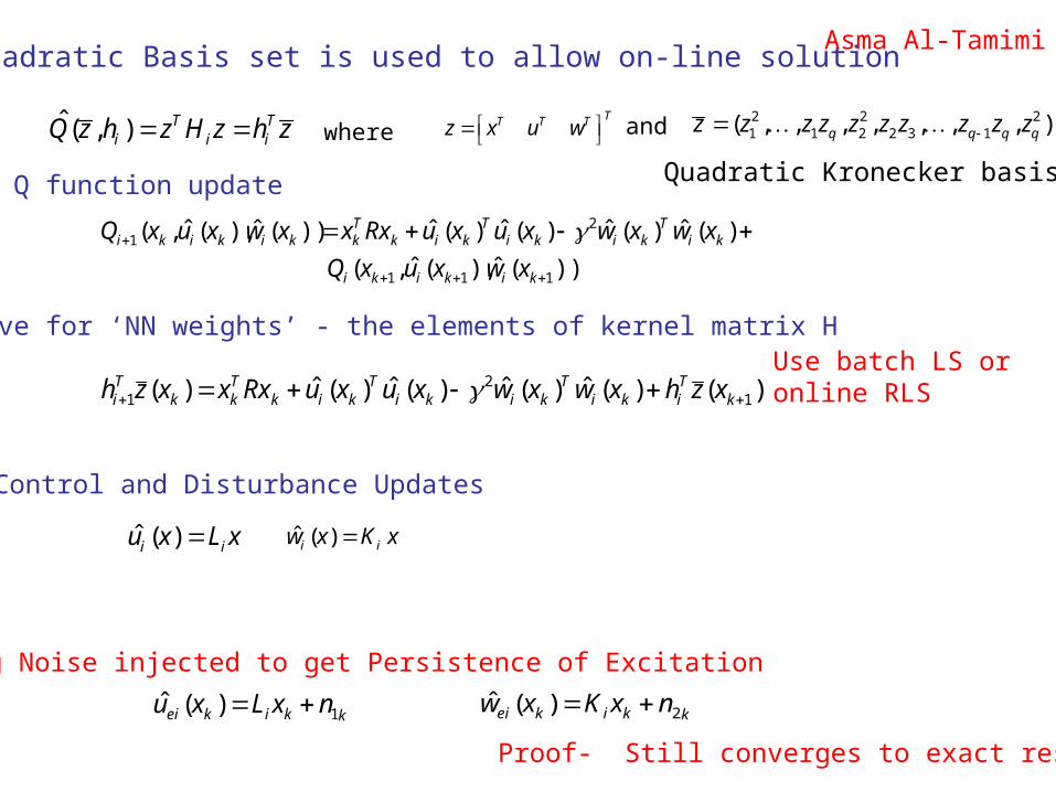
ˆ ( , ) T Ti i iQ z h z H z h z

ˆ ( )i iu x L x ˆ ( )i iw x K x

Quadratic Basis set is used to allow on-line solution

TT T Tz x u w 2 2 21 1 2 2 3 1( , , , , , , , )q q q qz z z z z z z z z z

))(ˆ),(ˆ,(

)(ˆ)(ˆ)(ˆ)(ˆ))(ˆ),(ˆ,(

111

21

kikiki

kiT

kikiT

kikTkkikiki

xwxuxQ

xwxwxuxuRxxxwxuxQ

)()(ˆ)(ˆ)(ˆ)(ˆ)( 12

1 kTiki

Tkiki

Tkik

Tkk

Ti xzhxwxwxuxuRxxxzh

kkikei nxLxu 1)(ˆ kkikei nxKxw 2)(ˆ

Probing Noise injected to get Persistence of Excitation

Proof- Still converges to exact result

Q function update

Solve for ‘NN weights’ - the elements of kernel matrix HUse batch LS or online RLS

where and

Quadratic Kronecker basis

Asma Al-Tamimi

Control and Disturbance Updates

H-inf Q learning Convergence Proofs

,1

kk

kkkkxy

wEuBxAx

• Convergence – H-inf Q learning is equivalent to solving

without knowing the system matrices

• The result is a model free Direct Adaptive Controller that converges to an H-infinity optimal controller

• No requirement what so ever on the model plant matrices

EKBKAK

ELBLAL

EBA

H

EKBKAK

ELBLAL

EBA

I

I

Q

H

iii

iiii

T

iii

iiii2

1

00

00

00

Asma Al-Tamimi

Direct H-infinity Adaptive Control

Asma Al-Tamimi

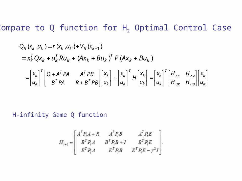
)(),(),( 1 khkkkkh xVuxruxQ

)()( kkT

kkkTkk

Tk BuAxPBuAxRuuQxx

k

k

uuux

xuxxT

k

k

k

kT

k

k

k

kTT

TTT

k

k

u

x

HH

HH

u

x

u

xH

u

x

u

x

PBBRPAB

PBAPAAQu

x

Compare to Q function for H2 Optimal Control Case

H-infinity Game Q function

Asma Al-Tamimi

ADP for Nonlinear Systems:Convergence Proof

HDP

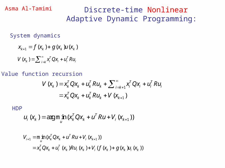
1 ( ) ( ) ( )k k k kx f x g x u x

( ) T Tk i i i ii k

V x x Qx u Ru

1

1

( )

( )

T T T Tk k k k k i i i ii k

T Tk k k k k

V x x Qx u Ru x Qx u Ru

x Qx u Ru V x

1( ) arg min( ( ))T Ti k k k i ku

u x x Qx u Ru V x

1 1min( ( ))

( ) ( ) ( ( ) ( ) ( ))

T Ti k k i ku

T Tk k i k i k i k k i k

V x Qx u Ru V x

x Qx u x Ru x V f x g x u x

Discrete-time NonlinearAdaptive Dynamic Programming:

HDP

Value function recursion

Asma Al-Tamimi

System dynamics

Asma Al-Tamimi

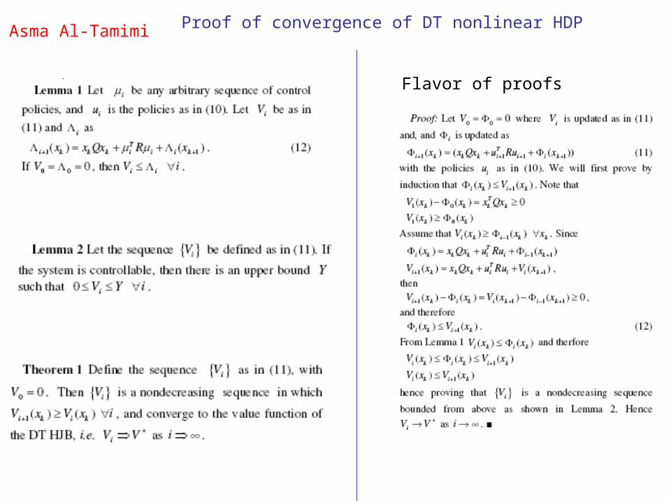
Flavor of proofs

Proof of convergence of DT nonlinear HDP

ˆ ( , ) ( )Ti k Vi Vi kV x W W x ˆ ( , ) ( )T

i k ui ui ku x W W x

1

1

ˆˆ ˆ( ( ), ) ( ) ( ) ( )

ˆ ˆ( ) ( ) ( )

T T Tk Vi k k i k i k i k

T T Tk k i k i k Vi k

d x W x Qx u x Ru x V x

x Qx u x Ru x W x

1( ) arg min( ( ))T Ti k k k i ku

u x x Qx u Ru V x

1 1min( ( ))

( ) ( ) ( ( ) ( ) ( ))

T Ti k k i k

u

T Tk k i k i k i k k i k

V x Qx u Ru V x

x Qx u x Ru x V f x g x u x

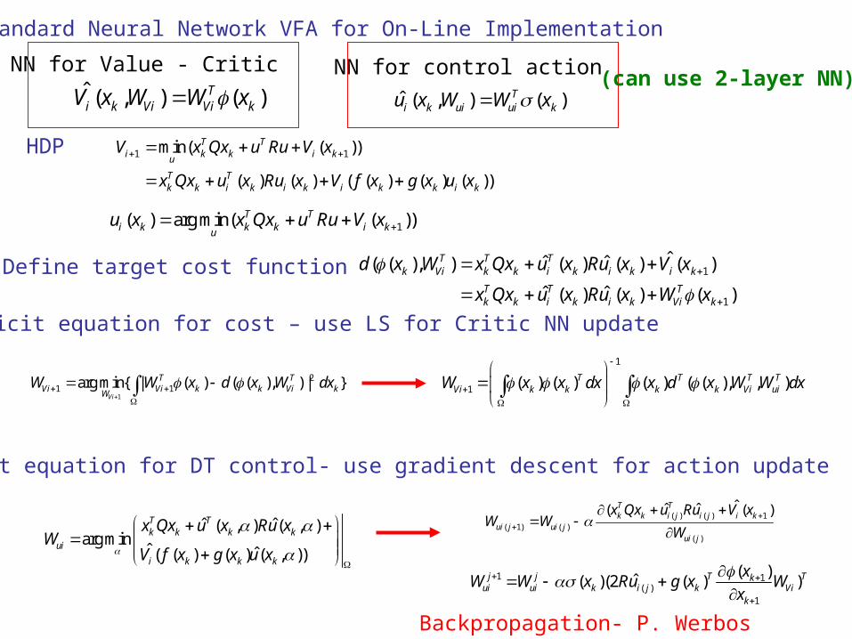
Standard Neural Network VFA for On-Line Implementation

Define target cost function

NN for Value - Critic NN for control action

HDP

Backpropagation- P. Werbos

Implicit equation for DT control- use gradient descent for action update

( ) ( ) 1( 1) ( )

( )

ˆˆ ˆ( ( )T Tk k i j i j i k

ui j ui jui j

x Qx u Ru V xW W

W

1 1( )

1

( )ˆ( )(2 ( ) )j j T Tk

ui ui k i j k Vik

xW W x Ru g x W

x

ˆ ˆ( , ) ( , )arg min

ˆ ˆ( ( ) ( ) ( , ))

T Tk k k k

ui

i k k k

x Qx u x Ru xW

V f x g x u x

1

21 1arg min{ | ( ) ( ( ), ) | }

Vi

T TVi Vi k k Vi kW

W W x d x W dx

Explicit equation for cost – use LS for Critic NN update

1

1 ( ) ( ) ( ) ( ( ), , )T T T TVi k k k k Vi uiW x x dx x d x W W dx

(can use 2-layer NN)

Batch LS

LS solution for Critic NN update

Issues with Nonlinear ADP

Integral over a region of state-spaceApproximate using a set of points

time

x1

x2

1

1 ( ) ( ) ( ) ( ( ), , )T T T TVi k k k k Vi uiW x x dx x d x W W dx

time

x1

x2

Take sample points along a single trajectory

Recursive Least-Squares RLS

Set of points over a region vs. points along a trajectory

Conjecture- For Nonlinear systemsThey are the same under a persistence of excitation condition

- Exploration

For Linear systems- these are the same

Selection of NN Training Set

Implicit equation for DT control- use gradient descent for action update

( ) ( ) 1( 1) ( )

( )

ˆˆ ˆ( ( )T Tk k i j i j i k

ui j ui jui j

x Qx u Ru V xW W

W

1 1( )

1

( )ˆ( )(2 ( ) )j j T Tk

ui ui k i j k Vik

xW W x Ru g x W

x

ˆ ˆ( , ) ( , )arg min

ˆ ˆ( ( ) ( ) ( , ))

T Tk k k k

ui

i k k k

x Qx u x Ru xW

V f x g x u x

ˆ ( , ) ( )Ti k ui ui ku x W W x

NN for control action

Note that state internal dynamics f(xk) is NOT needed in nonlinear case since:

1. NN Approximation for action is used

2. xk+1 is measured

Interesting Fact for HDP for Nonlinear systems

kjT

jT

kjkj AxPBBPBIxLxh 1)()( Linear Casemust know system A and B matrices

Draguna Vrabie

ADP for Continuous-Time Systems

Policy Iteration

HDP

),( uxfx

t

T

t

dtRuuxQdtuxrtxV ))((),())((

),,(),(),(),(),(0 ux

VxHuxruxf

x

Vuxrx

x

VuxrV

TT

0)0( V

),(),(min),(min0*

)(

*

)(uxf

x

Vuxrx

x

Vuxr

T

tu

T

tu

x

VxgRtxh T

*

12

1* )())((

dx

dVggR

dx

dVxQf

dx

dV T

TT *1

*

41

*

)(0

0)0( V

System

Cost

Hamiltonian

Optimal cost

Optimal control

HJB equation

Continuous-Time Optimal Control

Bellman

),(),(min),(min0)()(

uxfx

Vuxrx

x

Vuxr

T

tu

T

tu

)())(,()( 1 khkkkh xVxhxrxV

c.f. DT value recursion, where f(), g() do not appear

Linear system, quadratic cost -

System:

Utility:

The cost is quadratic

Optimal control (state feed-back):

HJB equation is the algebraic Riccati equation (ARE):

PBPBRQPAPA TT 10

)()()()( 1 tLxtPxxBRtu T

BuAxx

0,0;),( QRRuuQxxuxr TT

t

T tPxtxduxrtxV )()(),())((

),,(),(),(0 ux

VxHuxruxf

x

VT

))(,())(,(0 xhxrxhxfx

Vjj

Tj

0)0( jV

x

VxgRxh jT

j

)()( 12

11

CT Policy Iteration

• Convergence proved by Saridis 1979 if Lyapunov eq. solved exactly

• Beard & Saridis used complicated Galerkin Integrals to solve Lyapunov eq.

• Abu Khalaf & Lewis used NN to approx. V for nonlinear systems and proved convergence

RuuxQuxr T )(),(Utility

Cost for any given u(t)

Lyapunov equation

Iterative solution

Pick stabilizing initial control

Find cost

Update control

Full system dynamics must be known

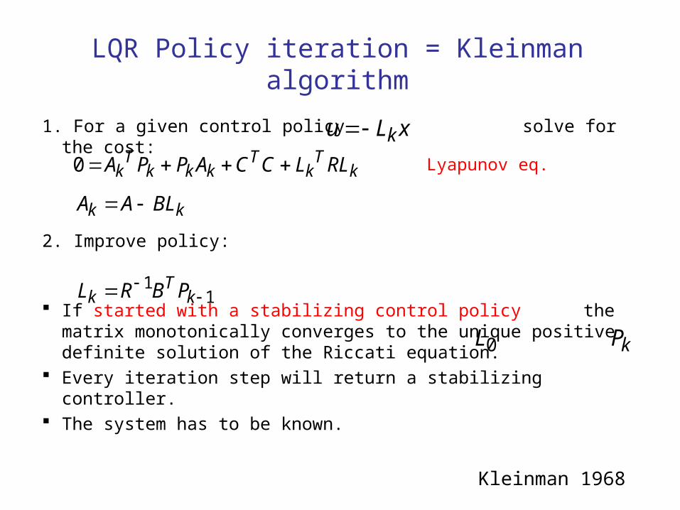
LQR Policy iteration = Kleinman algorithm

1. For a given control policy solve for the cost:

2. Improve policy:

If started with a stabilizing control policy the matrix monotonically converges to the unique positive definite solution of the Riccati equation.

Every iteration step will return a stabilizing controller. The system has to be known.

xLu k

kT

kT

kkkT

k RLLCCAPPA 0

11

k

Tk PBRL

kk BLAA

0L kP

Kleinman 1968

Lyapunov eq.

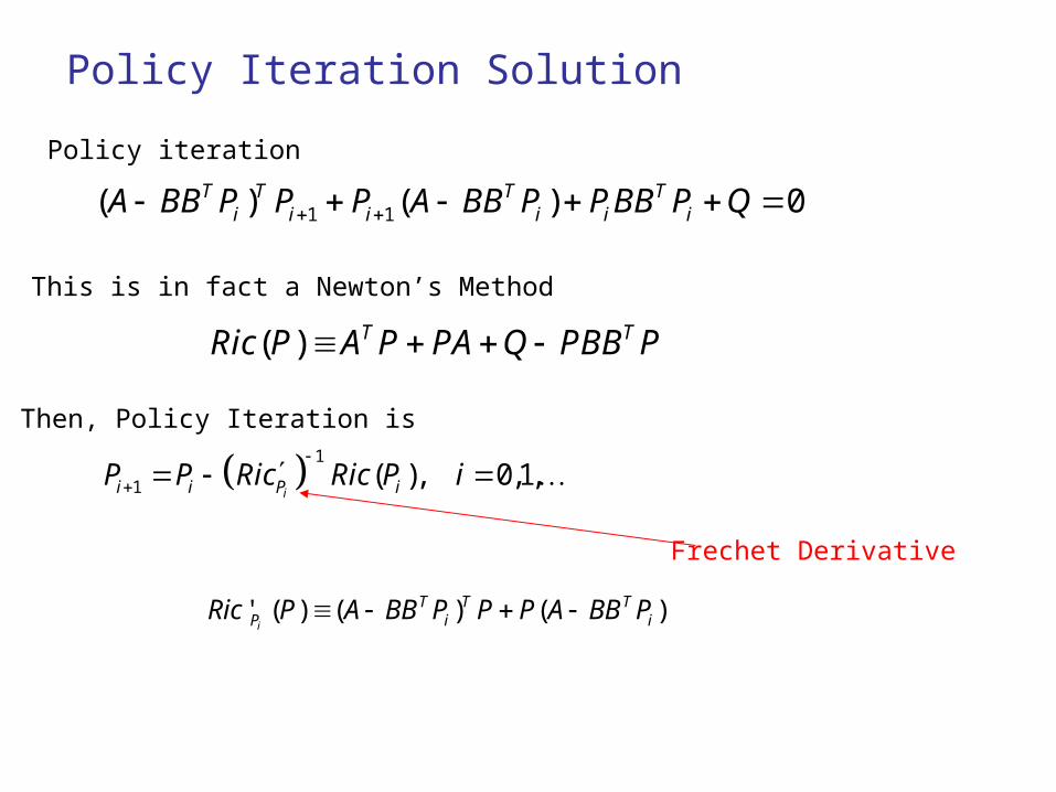
Policy Iteration Solution

( ) T TRic P A P PA Q PBB P

1 1( ) ( ) 0T T T Ti i i i i iA BB P P P A BB P PBB P Q

1

1 ( ), 0,1,ii i P iP P Ric Ric P i

Policy iteration

This is in fact a Newton’s Method

Then, Policy Iteration is

Frechet Derivative

)()()(' iTT

iT

P PBBAPPPBBAPRici

Synopsis on Policy Iteration and ADP

Need to know ONLY g(x) for control update

Either measure dx/dt or must know f(x), g(x)

If xk+1 is measured, do not need knowledge of f(x) or g(x))]()()([))(,(

)())(,()(

1

111

kjkkjkjk

kjkjkkj

xhxgxfVxhxr

xVxhxrxV

Discrete-time

kjT

jT

jkj AxPBBPBILxh 1)()( Need to know f(xk) AND g(xk) for control update

Policy iteration

)())(,()( 11 kjkjkkj xVxhxrxV ADP Greedy cost update

Continuous-time

))(,()]()()([))(,(0 xhxrxhxgxfx

Vxhxrx

x

Vjj

Tj

j

Tj

x

VxgRxh jT

j

)()( 12

11

Policy iteration

What is Greedy ADP for CT Systems ??

Policy Iterations without Lyapunov Equations

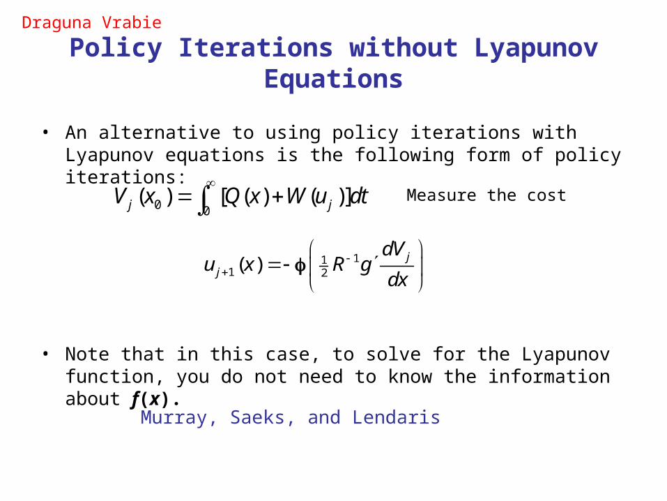
• An alternative to using policy iterations with Lyapunov equations is the following form of policy iterations:

• Note that in this case, to solve for the Lyapunov function, you do not need to know the information about f(x).

0 0( ) [ ( ) ( )]j jV x Q x W u dt

111 2( ) j

j

dVu x R g

dx

Murray, Saeks, and Lendaris

Measure the cost

Draguna Vrabie

Methods to obtain the solution

Dynamic programming built on Bellman’s optimality principle – alternative

form for CT Systems [Lewis & Syrmos 1995]

))(())(),((min))(( *

)(

* ttxVduxrtxVtt

tttt

u

)()()()())(),(( RuuQxxuxr TT

Solving for the cost – Our approach

))(()())(( TtxVdtRuuQxxtxVTt

t

TT

Lxu

Draguna Vrabie

f(x) and g(x) do not appear)())(,()( 1 khkkkh xVxhxrxV

c.f. DT case

For a given control

The cost satisfies

)()()()()( TtPxTtxdtRuuQxxtPxtx TTt

t

TTT

PBRL T1

LQR case

Optimal gain is

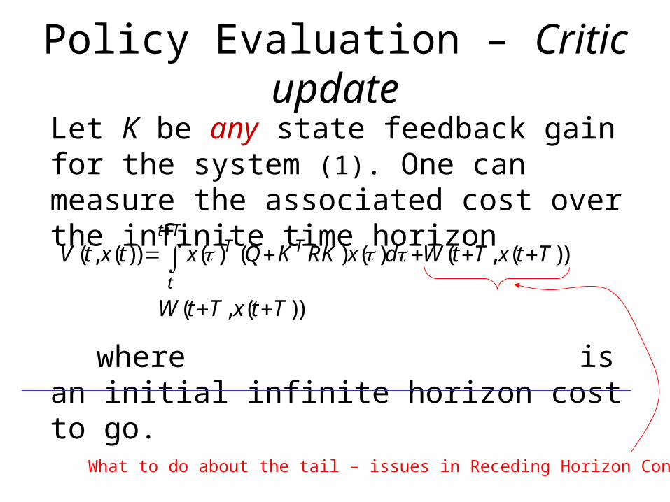
Policy Evaluation – Critic update

Let K be any state feedback gain for the system (1). One can measure the associated cost over the infinite time horizon

where is an initial infinite horizon cost to go.

( , ( )) ( ) ( ) ( ) ( , ( ))t T

T T

t

V t x t x Q K RK x d W t T x t T

( , ( ))W t T x t T

What to do about the tail – issues in Receding Horizon Control

Solving for the cost – Our approach

))(()())(( 001

0

0

TtxVdtRuuQxxtxV k

Tt

t

kTkTk

11010

0

0

)( xPxdtRuuQxxxPx kT

Tt

t

kTkTk

T

CT ADP Greedy iteration

)()( txLtu kk

11

1

kT

k PBRL

No initial stabilizing control needed

Now Greedy ADP can be defined for CT SystemsDraguna Vrabie

LQR

)()()()()( 11 TtxpdxPBBRPQxtxp T

i

Tt

ti

Ti

TTi

Control policy

Cost update

Control gain update

Implement using quadratic basis set

A and B do not appear

B needed for control update

Direct Optimal Adaptive Control for Partially Unknown CT Systems

u(t+T) in terms of x(t+T) - OK

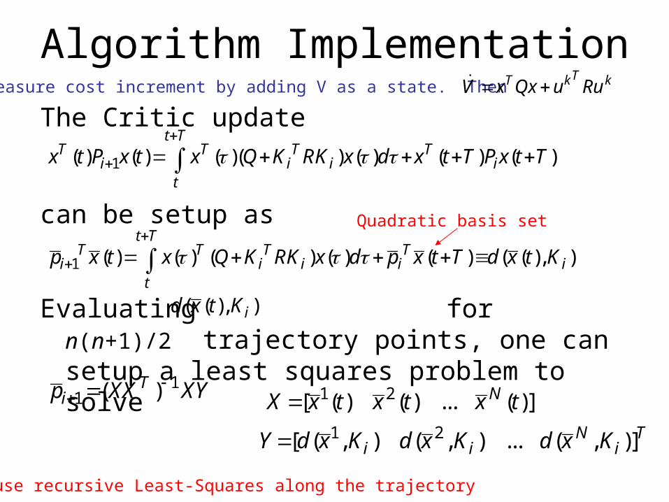
Algorithm Implementation

The Critic update

can be setup as

Evaluating for n(n+1)/2 trajectory points, one can setup a least squares problem to solve

1( ) ( ) ( )( ) ( ) ( ) ( )t T

T T T Ti i i i

t

x t P x t x Q K RK x d x t T P x t T

11 ( )T

ip XX XY 1 2[ ( ) ( ) ... ( )]NX x t x t x t

1 2[ ( , ) ( , ) ... ( , )]N Ti i iY d x K d x K d x K

( ( ), )id x t K

Or use recursive Least-Squares along the trajectory

1 ( ) ( ) ( ) ( ) ( ) ( ( ), )t T

T T T Ti i i i i

t

p x t x Q K RK x d p x t T d x t K

Quadratic basis set

Measure cost increment by adding V as a state. Then kTkT RuuQxxV

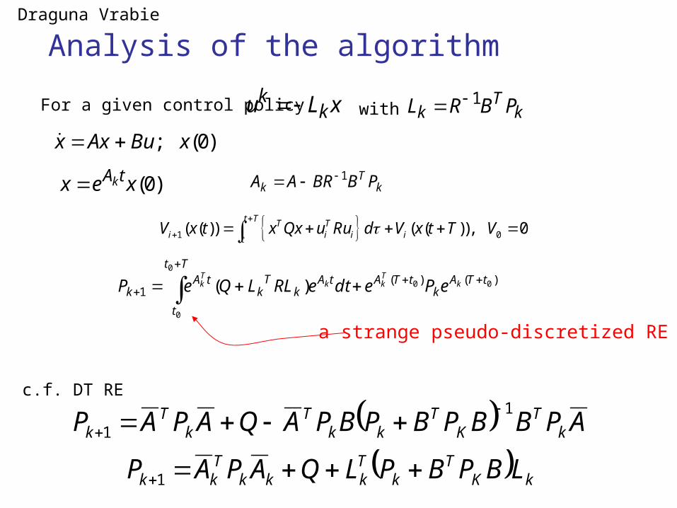
Analysis of the algorithm

For a given control policy

1 0( ( )) ( ( )), 0t T T T

i i i itV x t x Qx u Ru d V x t T V

xLu kk k

Tk PBRL 1

)0(xex tAk kT

k PBBRAA 1

)()(1

00

0

0

)( tTAk

tTATt

t

tAk

Tk

tAk

kTkk

Tk ePedteRLLQeP

)0(; xBuAxx

Greedy update is equivalent to

with

a strange pseudo-discretized RE

Draguna Vrabie

APBBPBPBPAQAPAP kT

KT

kkT

kT

k

1

1

c.f. DT RE

kKT

kTkkk

Tkk LBPBPLQAPAP 1

TtA

kT

kkktA

kk dteRLLQAPAPePP kTk

0

1 )(

Lemma 2. CT HDP is equivalent to

kT

k PBBRAA 1

ADP solves the CT ARE without knowledge of the system dynamics f(x)

Analysis of the algorithmDraguna Vrabie

This extra term means the initial Control action need not be stabilizing

When ADP converges, the resulting P satisfies the Continuous-Time ARE !!

Direct OPTIMAL ADAPTIVE CONTROL

Solve the Riccati Equation WITHOUT knowing the plant dynamics

Model-free ADP

Works for Nonlinear Systems

Proofs?Robustness?Comparison with adaptive control methods?

)()( txLtu kk

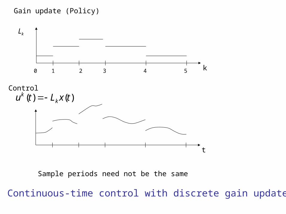
Continuous-time control with discrete gain updates

t

Lk

k0 1 2 3 4 5

Sample periods need not be the same

Gain update (Policy)

Control

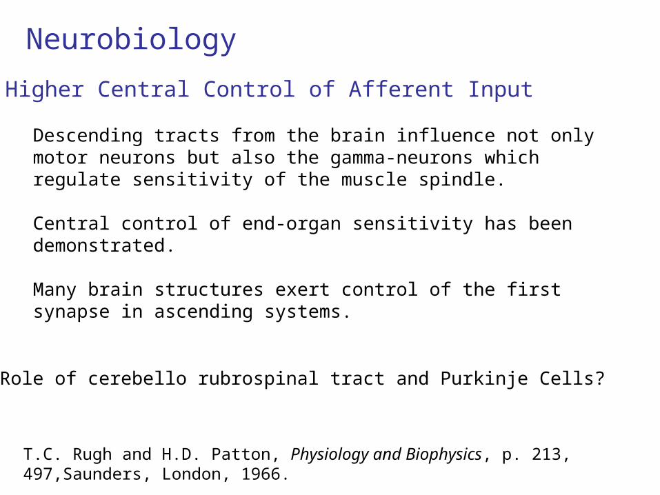
T.C. Rugh and H.D. Patton, Physiology and Biophysics, p. 213, 497,Saunders, London, 1966.

Higher Central Control of Afferent Input

Descending tracts from the brain influence not only motor neurons but also the gamma-neurons which regulate sensitivity of the muscle spindle.

Central control of end-organ sensitivity has been demonstrated.

Many brain structures exert control of the first synapse in ascending systems.

Role of cerebello rubrospinal tract and Purkinje Cells?

Neurobiology

t

uxr

t

VVuxr

t

VVuxrxVu

x

VxH tt

Dtttt

),(

),(),()(),,( 11

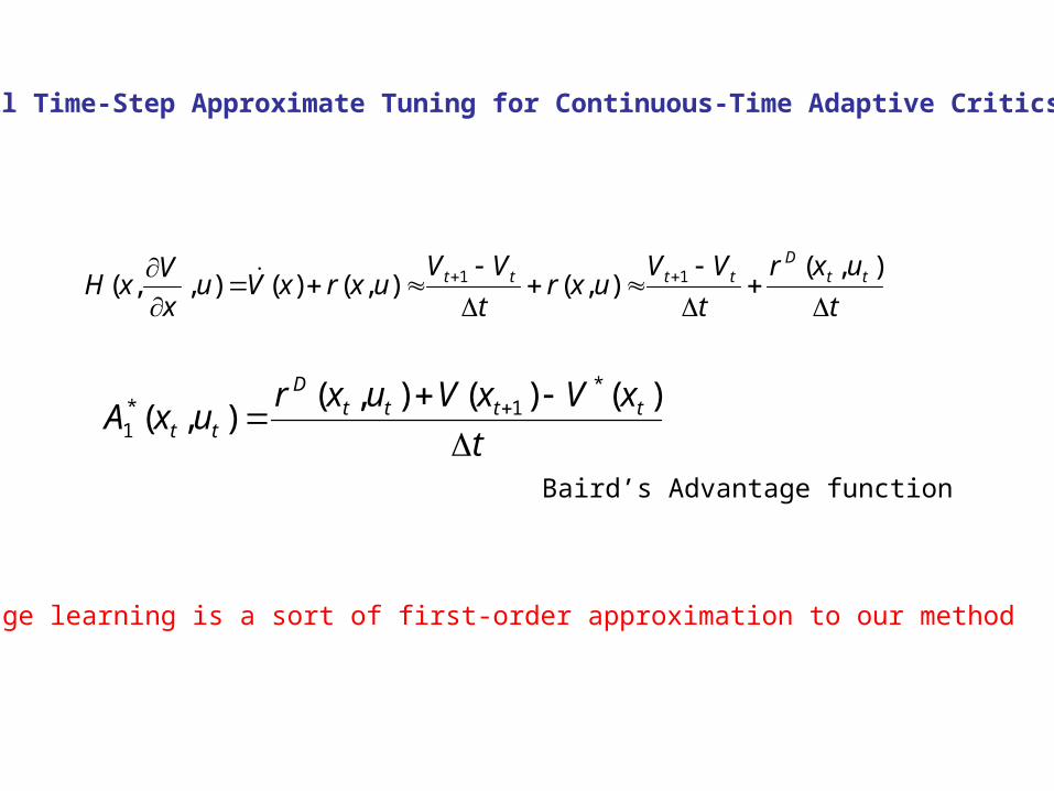
Small Time-Step Approximate Tuning for Continuous-Time Adaptive Critics

t

xVxVuxruxA tttt

D

tt

)()(),(),(

*1*

1

Baird’s Advantage function

Advantage learning is a sort of first-order approximation to our method

Results comparing the performances of DT-ADHDP and CT-HDP

Submitted to IJCNN’07 Conference Asma Al-Tamimi and Draguna Vrabie

System, cost function, optimal solution

System – power plant Cost

CARE:

-0.665 8 0 0

0 3.663 3.663 0

6.86 0 13.736 13.736

6 0 0 0

0 0 13.736 0T

A

B

Wang, Y., R. Zhou, C. Wen - 1993

,n mx Ax Bu x R u R

0.4750 0.4766 0.0601 0.4751

0.4766 0.7831 0.1237 0.3829

0.0601 0.1237 0.0513 0.0298

0.4751 0.3829 0.0298 2.3370

CAREP

1 0T TA P PA PBR B P Q

;n mQ I R I

*0

( )0

( ) min ( )T T

u tV x x Qx u Ru d

CT HDP results

0.4753 0.4771 0.0602 0.4770

0.4771 0.7838 0.1238 0.3852

0.0602 0.1238 0.0513 0.0302

0.4770 0.3852 0.0302 2.3462

CT HDPP

0 10 20 30 40 50 60-0.5

0

0.5

1

1.5

2

2.5P matrix parameters P(1,1),P(1,3),P(2,4),P(4,4)

Time (s)

P(1,1)P(1,3)P(2,4)P(4,4)

Convergence of the P matrix parameters for CT HDP

The state measurements were taken at each 0.1s time period.

A cost function update was performed at each 1.5s.

For the 60s duration of the simulation a number of 40 iterations (control policy updates) were performed.

*0

( )0

( ) min ( )T TCT CT

u tV x x Q x u R u d

0.4802 0.4768 0.0603 0.4754

0.4768 0.7887 0.1239 0.3834

0.0603 0.1239 0.0567 0.0300

0.4754 0.3843 0.0300 2.3433

DT ADHDPP

DT ADHDP results

Convergence of the P matrix parameters for DT ADHDP

The state measurements were taken at each 0.01s time period.

A cost function update was performed at each .15s.

For the 60s duration of the simulation a number of 400 iterations (control policy updates) were performed.

0 10 20 30 40 50 60-0.5

0

0.5

1

1.5

2

2.5

Time (s)

P matrix parameters P(1,1),P(1,3),P(2,4),P(4,4)

P(1,1)P(1,3)P(2,4)P(4,4)

[ , ]

* ( ) min ( ) ( )t k

T Tk t CT t t CT tt ku

V x x Q T x u R T u

Continuous-time used only 40 iterations!

The discrete version was obtained by discretizing the continuous time model using zero-order hold method with the sample time T=0.01s.

• CT HDP – Partially model free (the system A matrix is not

required to be known)

• DT ADHDP – Q learning– Completely model free

The DT ADHP algorithm is computationally more intensive than the CT HDP since it is using a smaller sampling period

Comparison of CT and DT ADP

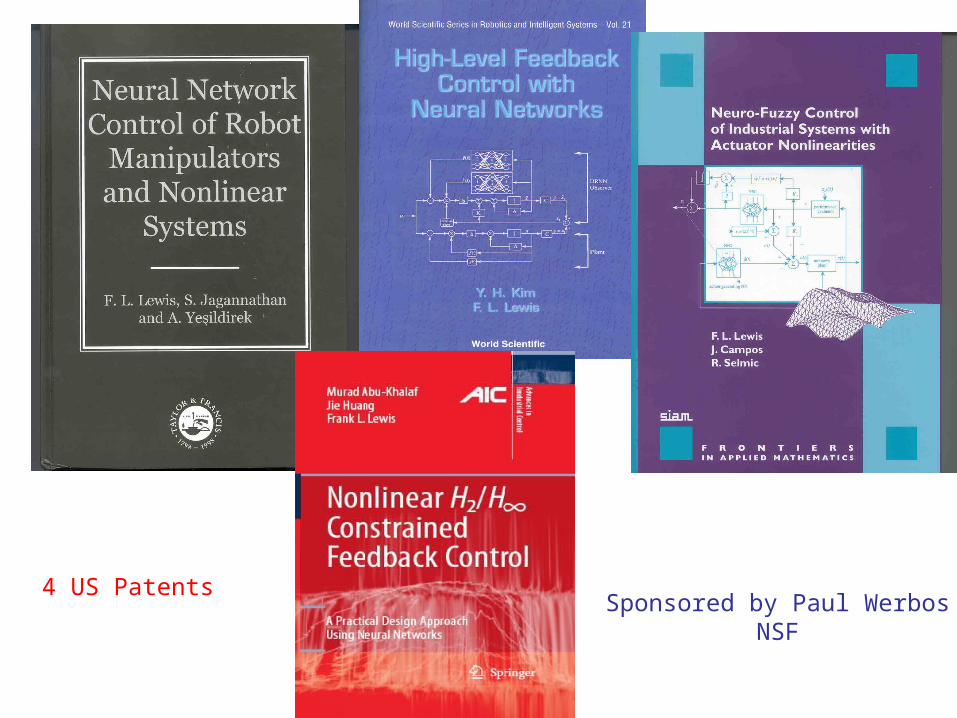
4 US PatentsSponsored by Paul Werbos

NSF

Call for Papers

IEEE Transactions on Systems, Man, & Cybernetics- Part B

Special Issue on

Adaptive Dynamic Programming and Reinforcement Learningin Feedback Control

George LendarisDerong LiuF.L Lewis

Papers due 1 August 2007