autonomous energy grid optimization - nrel.gov · pdf filesteven low nrel, september 2017 ....

Autonomous Energy Grid optimization

Steven Low

NREL, September 2017

Risk: active DERs introduce rapid random fluctuations in supply, demand, power quality increasing risk of blackouts

Opportunity: active DERs enables realtime dynamic network-wide feedback control, improving robustness, security, efficiency

Caltech research: distributed control of networked DERs

•  Foundational theory, practical algorithms, concrete applications •  Integrate engineering and economics •  Active collaboration with industry

Autonomous energy grid

Computational challenge n  nonlinear models, nonconvex optimization

Scalability challenge n  billions of intelligent DERs

Increased volatility n  in supply, demand, voltage, frequency

Limited sensing and control n  design of/constraint from cyber topology

Incomplete or unreliable data n  local state estimation & system identification

Data-driven modeling and control n  real-time at scale

many other important problems, inc. economic, regulatory, social, ...

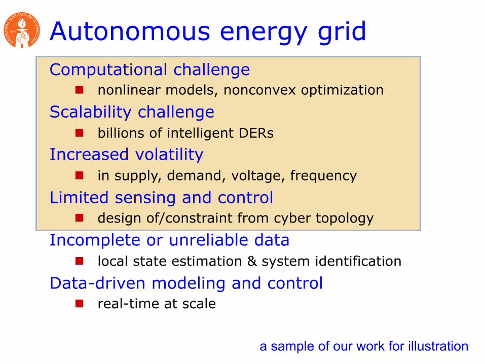
Autonomous energy grid

Computational challenge n  nonlinear models, nonconvex optimization

Scalability challenge n  billions of intelligent DERs

Increased volatility n  in supply, demand, voltage, frequency

Limited sensing and control n  design of/constraint from cyber topology

Incomplete or unreliable data n  local state estimation & system identification

Data-driven modeling and control n  real-time at scale

a sample of our work for illustration

Outline

Relaxations of AC OPF n  Dealing with nonconvexity

Distributed AC OPF n  Dealing with scalability

Realtime AC OPF n  Dealing with volatility

Optimal placement n  Dealing with limited sensing/control

Relaxations of AC OPF dealing with nonconvexity

Low, Convex relaxation of OPF, 2014

http://netlab.caltech.edu

Bose (UIUC) Chandy Farivar (Google) Gan (FB) Lavaei (UCB)

many others at & outside Caltech …

Li (Harvard)

Optimal power flow (OPF)

Computational challenge n  OPF underlies numerous power system applications but

is nonconvex (and NP-hard) Scalability challenge

n  Future smart grid will have billions of intelligent distributed energy resources (DERs)

Our approach n  Computation: developed relaxation theory that exploits

hidden convexity structure n  Scalability: developed distributed algorithms

implementable by DERs based on relaxation

Optimal power flow (OPF) min generation cost, network loss

generation limits

voltage constraints

sj = tr YjHVV H( ) for node jpower flow equations:

•  describes network topology and impedances

•  is net power injection (generation) at node j •  “power balance at each node j” (Kirchhoff’s law)

YjH

sj

minV∈Cn

tr CVV H( )s. t. s j ≤ tr Yj

HVV H( ) ≤ sj v j ≤ Vj

2 ≤ vj

C, Yj ∈Cn×n, s j, sj ∈C, v j,vj ∈ R

Optimal power flow (OPF)

minV∈Cn

tr CVV H( )s. t. s j ≤ tr Yj

HVV H( ) ≤ sj v j ≤ Vj

2 ≤ vj

min generation cost, network loss

generation limits

voltage constraints

nonconvex feasible set

•  not Hermitian (nor positive semidefinite)

•  is positive semidefinite (and Hermitian) nonconvex QCQP

YjH

C

Multiple solutions

11/66

[Ian Hiskens]

min tr CW

subject to s j ≤ tr YjHW( ) ≤ s j v j ≤Wjj ≤ vj

W ≥ 0, rank W =1

Equivalent problem:

Equivalent feasible sets

convex in W except this constraint

quadratic in V linear in W

min tr CVV H

subject to s j ≤ tr YjHVV H( ) ≤ s j v j ≤ |Vj |2 ≤ vj

V

Solution strategy

relaxation: minx∈X+

f x( )

OPF: minx∈X

f x( )

If optimal solution satisfies easily checkable conditions, then optimal solution of OPF can be recovered

x*x*

Equivalent relaxations

W+ WG+

V W WG

For radial networks: always solve SOCP !

Theorem n  Radial G: SOCP is equivalent to SDP ( ) n  Mesh G: SOCP is strictly coarser than SDP

V⊆W+ ≅WG+

Exact relaxation

For radial networks, sufficient conditions on n  power injections bounds, or n  voltage upper bounds, or n  phase angle bounds

Exact relaxation

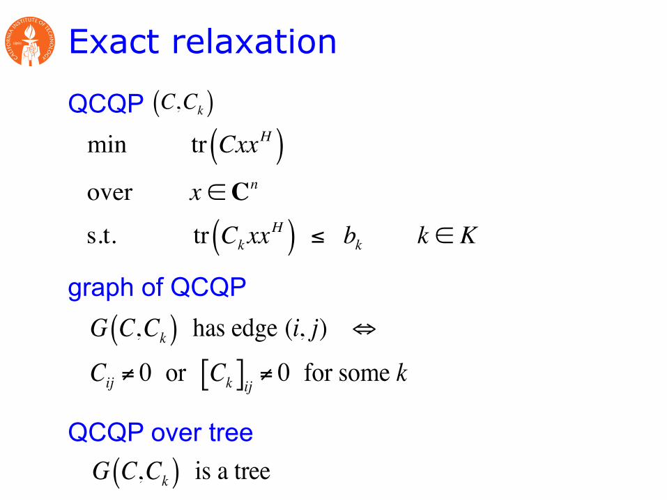
graph of QCQP G C,Ck( ) has edge (i, j) ⇔

Cij ≠ 0 or Ck[ ]ij ≠ 0 for some k

QCQP

QCQP over tree G C,Ck( ) is a tree

C,Ck( )min tr CxxH( )over x ∈Cn

s.t. tr CkxxH( ) ≤ bk k ∈ K

Exact relaxation

min tr CxxH( )over x ∈Cn

s.t. tr CkxxH( ) ≤ bk k ∈ K

Key condition i ~ j : Cij, Ck[ ]ij , ∀k( ) lie on half-plane through 0

QCQP C,Ck( )

Theorem SOCP relaxation is exact for QCQP over tree

Re

Im

Bose et al 2012, 2014 Sojoudi, Lavaei 2013

Implication on OPF

IEEE TRANS. ON CONTROL OF NETWORK SYSTEMS, 2014 5

[Y j] jk = �12(b jk + ig jk)

[Yk] jk = �12(b jk � ig jk)

as well as the angles of �[F j] jk,�[Fk] jk and�[Y j] jk,�[Yk] jk. These quantities are shown in Figure1 with their magnitudes normalized to a common value andexplained in the caption of the figure.

Φ j"# $% jk

Re

Im

− Φ j#$ %& jk

Φk[ ] jk

− Φk[ ] jk

Ψ j"# $% jk − Ψ k[ ] jk

Ψ k[ ] jk − Ψ j#$ %& jk

lower)bounds)on))pj,qj, pk,qk

α jk

[C0 ] jk

upper)bounds)on))pj,qj, pk,qk

Fig. 1: Condition A2’ on a line ( j,k) 2 E. The quantities([F j] jk, [Fk] jk, [Y j] jk, [Yk] jk) on the left-half plane corre-spond to finite upper bounds on (p j, pk,q j,qk) in (16a)–(16b); (�[F j] jk,�[Fk] jk,�[Y j] jk,�[Yk] jk) on the right-halfplane correspond to finite lower bounds on (p j, pk,q j,qk).A2’ is satisfied if there is a line through the origin, specifiedby the angle a jk, so that the quantities corresponding tofinite upper or lower bounds on (p j, pk,q j,qk) lie on oneside of the line, possibly on the line itself. The load over-satisfaction condition in [25], [29] corresponds to the Im-axis that excludes all quantities on the right-half plane. Thesufficient condition in [28, Theorem 2] corresponds to thered line in the figure that allows a finite lower bound on thereal power at one end of the line, i.e. p j or pk but not both,and no finite lower bound on reactive power q j.

Condition A2 applied to OPF (16) takes the following form(see Figure 1):A2’: For each link ( j,k) 2 E there is a line in the complex

plane through the origin such that [C0] jk as well asthose ±[Fi] jk and ±[Yi] jk corresponding to finite loweror upper bounds on (pi,qi), for i = j,k, are all on oneside of the line, possibly on the line itself.

Let Copt and Csocp denote the optimal values of OPF (2) andOPF-socp (7) respectively.

Corollary 3: Suppose G is a tree and A2’ holds.1) Copt =Csocp. Moreover an optimal solution V opt of OPF

(2) can be recovered from every optimal solution W socpG

of OPF-socp (7).2) If, in addition, A1 holds then OPF-socp (7) is exact.

It is clear from Figure 1 that condition A2’ cannot be satis-fied if there is a line where both the real and reactive powerinjections at both ends are both lower and upper bounded(8 combinations as shown in the figure). A2’ requires thatsome of them be unconstrained even though in practice theyare always bounded. It should be interpreted as requiringthat the optimal solutions obtained by ignoring these boundsturn out to satisfy these bounds. This is generally differentfrom solving the optimization with these constraints butrequiring that they be inactive (strictly within these bounds)at optimality, unless the cost function is strictly convex. Theresult proved in [26] also includes constraints on real branchpower flows and line losses. Corollary 3 includes severalsufficient conditions in the literature for exact relaxation asspecial cases; see the caption of Figure 1.

Corollary 3 also implies a result first proved in [16], usinga different technique, that SOCP relaxation is exact in BFMfor radial networks when there are no lower bounds on powerinjections s j. The argument in [16] is generalized in [17, PartI] to the case with convex objective functions, shunt elements,and line limits in terms of upper bounds on ` jk. Assume

A3: The cost function C(x) is convex, strictly increasingin `, nondecreasing in s = (p,q), and independent ofbranch flows S = (P,Q).

A4: For j 2 N+, s j =�•� i•.

Popular cost functions in the literature include active powerloss over the network or active power generations, both ofwhich satisfy A3. The next result is proved in [16], [17].

Theorem 4: Suppose G is a tree and A3–A4 hold. ThenOPF-socp (13) is exact.

Remark 2: If the cost function C(x) in A3 is only nonde-creasing, rather than strictly increasing, in `, then A3–A4still guarantee that all optimal solutions of OPF (10) are(i.e., can be mapped to) optimal solutions of OPF-socp (13),but OPF-socp may have an optimal solution that maintainsstrict inequalities in (11c) and hence is infeasible for OPF.Even though OPF-socp is not exact in this case, the proof ofTheorem 4 constructs from it an optimal solution of OPF.

B. Voltage upper bounds

While type A conditions (A2’ and A4 in the last sub-section) require that some power injection constraints not bebinding, type B conditions require non-binding voltage upperbounds. They are proved in [31], [32], [33], [34] using BFM.

For radial networks the model originally proposed in [18],which is (11) with the inequalities in (11c) replaced byequalities, is exact. This is because the cycle condition (12)is always satisfied as the reduced incidence matrix B is n⇥nand invertible for radial networks. Following [34] we adoptthe graph orientation where every link points towards node

Not both lower & upper bounds on real & reactive powers at both ends of a line can be finite

Example 25

(a) (b)

Fig. 4: Projections of feasible regions on p1 � p2 space for 3-bus system in (3).

P1

P2

0.42 0.43 0.44 0.45 0.46 0.47 0.48 0.49

0.48

0.49

0.5

0.51

0.52

0.53

0.54

h1(F+2 )

h1(F+1 )

h1(F1) = h1(F2)

Fig. 5: Zoomed in Pareto fronts of the 3-bus case in p1 � p2 space.

B. IEEE benchmark systems

For IEEE benchmark systems [35], [42], we solve R1, R2 and Rch in MATLAB using CVX

[43] with the solver SeDuMi [44]. The objective values and running times are presented in

Table II. As in Theorem 1, the problems R1 and Rch have the same objective function value,

i.e., r⇤1 = r⇤ch. However, the optimal objective value of R2 is lower, i.e., r⇤2 < r⇤1. For IEEE

benchmark systems, note that R1 and Rch are exact [14]–[16], while R2 is not. As evidenced

by the running times in Table II, Rch is much faster than R1. The chordal extension of the

May 31, 2013 DRAFT

26

(a) (b)

graphs are computed in advance for each case using the algorithm in [45]. R2 is faster than both

R1 and Rch, but yields an infeasible solution for most IEEE benchmark systems considered.

TABLE II: Comparing objective values and running times on IEEE systems

Test case Objective value Running times

R1, Rch R2 R1 Rch R2

9 bus 5297.4 5297.4 0.2 0.2 0.2

14 bus 8081.7 8075.3 0.2 0.2 0.2

30 bus 574.5 573.6 0.4 0.3 0.3

39 bus 41889.1 41881.5 0.7 0.3 0.3

57 bus 41738.3 41712.0 1.3 0.5 0.3

118 bus 129668.6 129372.4 6.9 0.7 0.6

300 bus 720031.0 719006.5 109.4 2.9 1.8

2383 bus 1840270 1789500.0 - 1005.6 155.3

VI. CONCLUSION

TBD

(Bose says: I think it’s better to talk about this in the conclusion.) (Steven says: Summary

about specific relaxations: SDP = chordal tighter than SOCP; BFM = BIM, SOCP in BFM =

SOCP in BIM; equivalence of feasible sets. Or summarize these in Conclusion section?)

May 31, 2013 DRAFT

power flow solution X

SDP Y SOCP Y

Real Power Reactive Power

•  Relaxation is exact if X and Y have same Pareto front

•  SOCP is faster but coarser than SDP

Bose, Low, Teeraratkul, Hassibi TAC 2015

Fig. 1: J(Xk) vs # of Iterations (Bisection Method) (a) 3-Bus Example (b) 5-Bus Example, (c) Modified IEEE 14 Bus Example (14B)

optimal point (Column 3) typically in a small number of iter-ations (Column 4). Thus the optimal cost for the semidefiniterelaxation, J�, is in fact equal to the optimal cost of the OPFproblem. Moreover, the rank-one solution returned from thelinearization-minimization algorithm can be used to constructan optimal solution for the non-convex OPF problem. Theseresults verify that primal/dual solvers will fail to return rank-one optimal solutions for the naive semidefinite relaxationeven when such solutions exist (c.f. Theorem 2.1). The valuesof J in the last column denote the upper bound on theoptimal cost of the OPF problem given by the non-convexsolver MATPOWER [3]. The last result in Table III is ofparticular interest. This example is a modified IEEE 14Bus system (14A) for which the linearization-minimizationalgorithm yields a rank-one globally optimal solution witha cost 12.4% lower than the sub-optimal solution obtainedwith MATPOWER. This example was constructed from thestandard IEEE 14 Bus test case [22] by tightening a subsetof the line capacity constraints. A precise description can befound in [23].

TABLE III: Power system examples with hidden rank-one opti-mal solutions. Precise systems descriptions can beobtained from (9 bus [24]), (30 bus [25]) (118 bus[22]), (14A bus [23]).

Syst. rank(X0

) rank(X0

) Iter. J� J

9 8 1 3 5296.7 5296.730 9 1 3 576.9 576.9118 236 1 100 129661 129661

14A 26 1 3 8092.8 9093.8

B. Alternating-Bisection Method

For certain problems, the linearization-minimization al-gorithm fails to uncover a rank-one point in F – i.e.rank(X

0

) > 1. In such cases, one of two scenarios couldbe at play. Either the optimal face F of the semidefiniterelaxation does not possess a rank-one matrix or the rankminimization heuristic may simply fail in recovering a rank-one points in F when they do in fact exist. Table IVprovides three representative examples of such cases. Foreach example, the rank minimization heuristic is able tofind a lower rank matrix (on F) than that achieved by the

naive semidefinite relaxation. However, the iteration doesnot converge to a rank-one solution. In each case there is anon-zero gap between the cost achieved for the semidefiniterelaxation, J�, and the MATPOWER upper bound obtainedfor the original OPF problem, J .

The alternating bisection-minimization method is applied tothe cases in Table IV. Figure 1 depicts the cost of a feasiblepoint produced at every step of the bisection for the examplesconsidered in Table IV. The red diamonds denote the iteratesachieving rank-one feasible points, while the black circlesdenote iterates corresponding to high rank feasible points.We observe in Figure 1, that in the case of the three andfive bus examples, the minimum cost obtained by a rank-one feasible point through bisection coincides with the costproduced by MATPOWER. This may lead one to believethat the optimal face F of the semidefinite relaxation maynot admit a rank-one feasible point. On the other hand, forthe modified IEEE 14 Bus example (14B), the proposedbisection-minimization heuristic obtains a rank-one feasiblepoint that yields a substantially lower cost than the upperbound J obtained from MATPOWER. More precisely, theminimum cost rank-one point derived from the alternatingbisection-minimization method is within 0.1266% of therelaxed lower bound J�, as compared to 4.8326% for theMATPOWER solution. We refer the reader to Remark 6 fora discussion on the role of mild constraint relaxations inderiving nearly optimal rank-one solutions.

To summarize, we observe that in many cases the iterativelinearization-minimization algorithm successfully uncovers ahidden rank-one point that is also globally optimal for theoriginal OPF problem. If the rank minimization algorithmfails to uncover a rank-one optimal point, then the alternatingbisection-minimization method can be applied. In this case,a rank-one feasible solution is obtained that yields a costthat is no greater than that achieved by MATPOWER – andfor certain systems, achieves a substantially lower cost thanMATPOWER.

V. CONCLUSION AND FUTURE DIRECTIONS

This paper considered the non-convex Optimal Power Flow(OPF) problem and the corresponding semidefinite relax-ation. For certain power systems and cost structures, thenaive semidefinite relaxation may fail to yield low rank

SDPcost

MATPOWERcost

IEEE test systems

12.4%lowercostthansolu=onfromnonlinearsolverMATPOWER

Potential benefits

[Louca, Seiler, Bitar 2013]

Potential benefits

Our research n  Computation: developed relaxation theory that exploits

hidden convexity structure n  Scalability: developed distributed algorithms

implementable by DERs based on relaxation theory n  Benefits: captures values to both utility and users

optimized baseline

peak load reduction: 8% energy cost reduction: 4%

exactness

Convex relaxations of OPF

distributed OPF

Kim, Baldick 1997 Dall’Anese et al 2012 Lam et al 2012 Kraning et al 2013 Devane, Lestas 2013 Sun et al 2013 Li et al 2013 Peng, Low 2014

moment/SoS, based

relaxation Molzahn, Hiskens 2014 Josz et al 2014 Ghaddar et al 2014

multiphase unbalanced

Dall’Anese et al 2012 Gan, Low 2014

applications

B&B, rank min,

QC relaxation,

Phan 2012 Gopalakrishnan 2012 Louca et al 2013 Hijazi et al 2013 Andy Sun 2016

ext refs in tutorial: Low, TCNS 2014

http://netlab.caltech.edu

semidefinite relaxations

Challenges

Challenges for practical application n  Relaxation may not be exact

o  Practical application demands a feasible solution o  No known sufficient condition for exact relaxation

for general mesh (transmission) networks n  Semidefinite relaxation (as is) is not scalable

Distributed AC OPF for scalability

Peng (Google)

Gan & L, PSCC 2014 Peng & L, TSG 2017

Gan (FB)

Summary: 3 ideas

1. Solve semidefinite relaxation using branch-flow model (BFM)

n  BFM much more numerically stable n  assume relaxation is exact (radial nk)

2. Decouple into operations at each bus n  introduce decoupling variables and consensus

constraints n  message passing between neighboring buses

3. Apply ADMM n  derive closed-form solution or 6x6 eigenvalue

problem for each ADMM subproblem n  greatly speeds up each ADMM iteration

Summary: simulations

BFM is much more numerically stable SDP relaxations are exact (wye loads)

numerically unstable

numerically stable

network

BIM-SDP BFM-SDP

value time ratio value time ratio

IEEE 13-bus 152.7 1.05 8.2e-9 152.7 0.74 2.8e-10

IEEE 34-bus -100.0 2.22 1.0 279.0 1.64 3.3e-11

IEEE 37-bus 212.3 2.66 1.5e-8 212.2 1.95 1.3e-10

IEEE 123-bus -8917 7.21 3.2e-2 229.8 8.86 0.6e-11

Rossi 2065-bus -100.0 115.50 1.0 19.15 96.98 4.3e-8

[Gan & Low 2014 PSCC]

Summary: comparison (single phase)

Network size N

Total Time S

Avg time ( = S/N )

Centralized (CPU)

Centralized (elapsed)

IEEE 123 buses

39.5 sec 0.32 sec 1.18 sec 11.4 sec

Rossi 2,065 1,153 0.56 14.38 157.3 1,313 471 0.36 8.88 91.2 792 226 0.29 5.13 50.3 363 66 0.18 3.08 24.5 108 16 0.14 0.78 6.5

footnote: “Centralized” times reported by CVS in Matlab n  Solving SOCP using CVX (not ADMM) n  “CPU” time excludes problem set up before calling convex solver n  “elapsed” time includes setup time in CVX

o  Parallel implementation of our distributed algorithm is much faster than solving OPF centrally

Summary: simulations Network (unbalanced)

n  IEEE 13, 34, 37, 123 bus systems Objective

n  loss minimization

Convergence time (computation only)

Network Diameter Iterations Total Time Avg Time 13 Bus 6 289 17.11 1.32 34 Bus 20 547 78.34 2.30 37 Bus 16 440 75.67 2.05 123 Bus 30 608 306.3 2.49

Details: 3 ideas

1. Solve semidefinite relaxation using branch-flow model (BFM)

n  BFM much more numerically stable n  assume relaxation is exact (radial nk)

2. Decouple into operations at each bus n  introduce decoupling variables and consensus

constraints n  message passing between neighboring buses

3. Apply ADMM n  derive closed-form solution or 6x6 eigenvalue

problem for each ADMM subproblem n  greatly speeds up each ADMM iteration

DistFlow model (Baran & Wu 1989)

minx

f (x) subject to DistFlow equations

operation constraints g(x) ≤ 0

OPF

nonconvex !

SOCP relaxation (Farivar & Low 2013) •  Equivalent re-formulation of DistFlow equations (linear + quadratic term) •  SOCP relaxation is often exact, yielding global optimal •  Much more numerically stable than bus injection model

1402

II. FORMULATION OF THE PROBLEM In this section, the network reconfiguration problems for both loss

reduction and load balancing are formulated and their similarities are pointed out.

2.1 Problem Statement To simplify the presentation, we will represent the system on a per

phase basis and the loads along a feeder section as constant P,Q loads placed at the end of the l ies. We also assume that every switch is associated with a line in the system. For example, we assume that the system of Fig.1 can be translated to an equivalent network shown in Fig.2.

ss1 m Figure 2: One line diagram of a small distribution system

In the figure, solid branches represent the lines that are in service and con- stitute the base radial configuration. Dotted branches (branches 20,2 1,22) represent the lines with open switches.

The base network can be reconfigured by first closing an open branch, say branch 21 in the figux. Since this switching will create a loop in the system, (composed of branches 1,2,3,21, 11, 10,9,8,7, and 15), a branch in the loop containing a switch has to be opened, say branch 7, to restore the radial structure of the system. As a result of this switching, the loads between the branches 7-1 1 will be transferred from one feeder to the Other. We will use the same terminology used in [7] and call t h i s basic switching operation a brunch exchange between branches 21 and 7. In general, as illustrated in the introduction, more complex switching schemes are possible; we will simulate such cases by applying several branch exchanges successively.

The load transfer between different substations can be simulated by branch-exchange type switchings too. In this case, substation nodes (node SSI and SS2 in the figure) will be considered as a common node although they are not the same node. The methods to be presented in this paper can handle both cases. This is an important property of the proposed methods.

The network rewnfiguration problems for loss reduction and load balancing involve the same type of operation, namely the load transfer between the feeders or substations by changing the positions of switches. They only differ in their objective. Other factors, such as the voltage profile of the system, capacities of the IinWtransformers, reliability con- . straints can be considered as constraints.

To state these problems as optimization pmblems, note that the radial configuration corresponds to a "spanning tree" of a graph represent- ing the network topology. Thus, we have a so-called minimal spanning tree problem which can be stated as follows. Given a graph, 6nd a spanning tree such that the objective function is minimized while the following constraints are satisfied: (i) voltage constraints, (ii) capacity constrains of liies/transformers. (iii) reliability constraints.

This is a combinatorial optimization problem since the solution involves the consideration of all possible spanning tms.

2.2 Power Flow Equations To calculate the terms in optimization problem defined in the previous

section, we will use a set of power flow equations that are structurally rich and conducive to computationally efficient solution schemes [13]. To illustrate them, consider the radial network in Fig.3.

...... T'1k..'....- i-1 i i+ 1 (-* P,.Q, - P ; f Q r - i mi i+i*Qi+i pn 'Qn

PL ,Qti

Figure 3 : One line diagram of a radial network

We represent the lines with impedances zl = r, + jx, , and loads as constant power sinks, SL =PL + jQL .

Power flow in a radial distribution network canhe described by a set of recursive equations, called D i s t F h branch equatwns , that use the real power, reactive power, and voltage magnitude at the sendhg end of a branch - Pi,Qi,Vi respectively to express the same quantities at the receiving end of the branch as follows.

p .2+Q 2

Vi' Pi,] =p i - ri - - "LI+I (1.i)

P?+Qi' Viz

VLl = Vi2 - 2(ri Pi + xi Q i ) + (r? + x?)- (1 .iii)

Hence, if P o .Qo , Vo at the Erst node of the network is known or estimated, then the same quantities at the other nodes can be calculated by applying the above branch equations successively. We shall =fer to this procedure as a forward update.

DistFlow branch equations can be written backward too. i.e., by using the real power, reactive power, and the voltage magnitude at the receiving end of a branch, P i , Q, , Vi to express the same quantities at the sending end of the branch. The result is the following recursive equations, called the backward branch equations,

P l - l = P l + f i T + P P , pl'2+Q,2 (2.i) v,

(2.ii)

where, PI' = Pi + Pti , Q; = Q, + QL; . Similar to forward update, a backward update can be defined: start

updating from the last node of the network assuming the variables Pn , Qn , Vn at that point are given and proceed backwards calculating the same quantities at the other nodes by applying Eq.(2) successively. Updat- ing process ends at the first node (node 0) and will provide the new estimate of the power injections into the network, PO .Qp

Note that by applying backward and forward update schemes successively one can get a power flow solution as explained in [131.

2 3 Calculation of the Objective Terms Having a network model, now we can express the power loss and

measure the load balance in the system in terms of system variables. For loss reduction, the objective is to minimize the total i2r losses in

the system, which can be calculated as follows.

(3)

This will be the objective function, cp of network reconfiguration for loss reduction.

For load balancing, we will use the ratio of complex power at the sending end of a branch, SI over its kVA capacity, Si"" as a measure of how much that branch is loaded. The branch can be a transformer. a tie- line with a sectionaliiing switch or simply a line section. Then we define the load 'balance index for the whole system as the sum of these measures, i.e.,

This will be the objective function, cb of load balancing. As noted before, the two problems are similar. They both require the

same data (system parameters and load) and load flow calculation to evaluate the objectives for a given network topology.

BFM and relaxations

DistFlow model (Baran & Wu 1989)

1402

II. FORMULATION OF THE PROBLEM In this section, the network reconfiguration problems for both loss

reduction and load balancing are formulated and their similarities are pointed out.

2.1 Problem Statement To simplify the presentation, we will represent the system on a per

phase basis and the loads along a feeder section as constant P,Q loads placed at the end of the l ies. We also assume that every switch is associated with a line in the system. For example, we assume that the system of Fig.1 can be translated to an equivalent network shown in Fig.2.

ss1 m Figure 2: One line diagram of a small distribution system

In the figure, solid branches represent the lines that are in service and con- stitute the base radial configuration. Dotted branches (branches 20,2 1,22) represent the lines with open switches.

The base network can be reconfigured by first closing an open branch, say branch 21 in the figux. Since this switching will create a loop in the system, (composed of branches 1,2,3,21, 11, 10,9,8,7, and 15), a branch in the loop containing a switch has to be opened, say branch 7, to restore the radial structure of the system. As a result of this switching, the loads between the branches 7-1 1 will be transferred from one feeder to the Other. We will use the same terminology used in [7] and call t h i s basic switching operation a brunch exchange between branches 21 and 7. In general, as illustrated in the introduction, more complex switching schemes are possible; we will simulate such cases by applying several branch exchanges successively.

The load transfer between different substations can be simulated by branch-exchange type switchings too. In this case, substation nodes (node SSI and SS2 in the figure) will be considered as a common node although they are not the same node. The methods to be presented in this paper can handle both cases. This is an important property of the proposed methods.

The network rewnfiguration problems for loss reduction and load balancing involve the same type of operation, namely the load transfer between the feeders or substations by changing the positions of switches. They only differ in their objective. Other factors, such as the voltage profile of the system, capacities of the IinWtransformers, reliability con- . straints can be considered as constraints.

To state these problems as optimization pmblems, note that the radial configuration corresponds to a "spanning tree" of a graph represent- ing the network topology. Thus, we have a so-called minimal spanning tree problem which can be stated as follows. Given a graph, 6nd a spanning tree such that the objective function is minimized while the following constraints are satisfied: (i) voltage constraints, (ii) capacity constrains of liies/transformers. (iii) reliability constraints.

This is a combinatorial optimization problem since the solution involves the consideration of all possible spanning tms.

2.2 Power Flow Equations To calculate the terms in optimization problem defined in the previous

section, we will use a set of power flow equations that are structurally rich and conducive to computationally efficient solution schemes [13]. To illustrate them, consider the radial network in Fig.3.

...... T'1k..'....- i-1 i i+ 1 (-* P,.Q, - P ; f Q r - i mi i+i*Qi+i pn 'Qn

PL ,Qti

Figure 3 : One line diagram of a radial network

We represent the lines with impedances zl = r, + jx, , and loads as constant power sinks, SL =PL + jQL .

Power flow in a radial distribution network canhe described by a set of recursive equations, called D i s t F h branch equatwns , that use the real power, reactive power, and voltage magnitude at the sendhg end of a branch - Pi,Qi,Vi respectively to express the same quantities at the receiving end of the branch as follows.

p .2+Q 2

Vi' Pi,] =p i - ri - - "LI+I (1.i)

P?+Qi' Viz

VLl = Vi2 - 2(ri Pi + xi Q i ) + (r? + x?)- (1 .iii)

Hence, if P o .Qo , Vo at the Erst node of the network is known or estimated, then the same quantities at the other nodes can be calculated by applying the above branch equations successively. We shall =fer to this procedure as a forward update.

DistFlow branch equations can be written backward too. i.e., by using the real power, reactive power, and the voltage magnitude at the receiving end of a branch, P i , Q, , Vi to express the same quantities at the sending end of the branch. The result is the following recursive equations, called the backward branch equations,

P l - l = P l + f i T + P P , pl'2+Q,2 (2.i) v,

(2.ii)

where, PI' = Pi + Pti , Q; = Q, + QL; . Similar to forward update, a backward update can be defined: start

updating from the last node of the network assuming the variables Pn , Qn , Vn at that point are given and proceed backwards calculating the same quantities at the other nodes by applying Eq.(2) successively. Updat- ing process ends at the first node (node 0) and will provide the new estimate of the power injections into the network, PO .Qp

Note that by applying backward and forward update schemes successively one can get a power flow solution as explained in [131.

2 3 Calculation of the Objective Terms Having a network model, now we can express the power loss and

measure the load balance in the system in terms of system variables. For loss reduction, the objective is to minimize the total i2r losses in

the system, which can be calculated as follows.

(3)

This will be the objective function, cp of network reconfiguration for loss reduction.

For load balancing, we will use the ratio of complex power at the sending end of a branch, SI over its kVA capacity, Si"" as a measure of how much that branch is loaded. The branch can be a transformer. a tie- line with a sectionaliiing switch or simply a line section. Then we define the load 'balance index for the whole system as the sum of these measures, i.e.,

This will be the objective function, cb of load balancing. As noted before, the two problems are similar. They both require the

same data (system parameters and load) and load flow calculation to evaluate the objectives for a given network topology.

BFM and relaxations

But DistFlow model is single-phase !

How to generalize to 3-phase unbalanced system? •  Preserve simple analytical structure of 1-phase model •  Preserve superior numerical stability of 1-phase model

DistFlow model for 1-phase

equivalent re-formulation

SOCP relaxation

generalization to 3-phase

SDP relaxation

Dall’Anese et al 2013 TSG Gan & Low 2014 PSCC (above approach)

radial, multiphase, wye + delta

Multiphase generalization

Zhao et al 2017 IREP

distributed solution

distributed solution

Peng & Low 2017 TSG Peng & Low 2015 CDC

3phase model

3-phase balanced

I jka

I jkb

I jkc

!

"

####

$

%

&&&&

=

yjkaa 0 0

0 yjkbb 0

0 0 yjkcc

!

"

####

$

%

&&&&

Vja

Vjb

Vjc

!

"

####

$

%

&&&&

−

Vka

Vkb

Vkc

!

"

###

$

%

&&&

(

)

****

+

,

----

per-phase analysis

I jka = yjk

aa Vja −Vk

a( )

3-phase unbalanced

I jka

I jkb

I jkc

!

"

####

$

%

&&&&

=

yjkaa yjk

ab yjkac

yjkba yjk

bb yjkbc

yjkca yjk

cb yjkcc

!

"

####

$

%

&&&&

Vja

Vjb

Vjc

!

"

####

$

%

&&&&

−

Vka

Vkb

Vkc

!

"

###

$

%

&&&

(

)

****

+

,

----

3-phase analysis

I jk = yjk Vj −Vk( )

3x3 matrix

(positive sequence)

(phase frame)

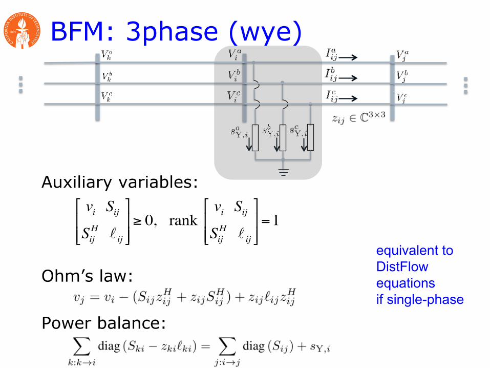
Auxiliary variables:

Ohm’s law:

Power balance:

vi SijSijH ℓ ij

!

"##

$

%&&≥ 0, rank

vi SijSijH ℓ ij

!

"##

$

%&&=1

BFM: 3phase (wye)

vi =ViViH ℓ ij = Iij Iij

H

Sij =ViIijH

3x3 rank-1 matrices


Ohm’s law:

Power balance:

vi SijSijH ℓ ij

!

"##

$

%&&≥ 0, rank

vi SijSijH ℓ ij

!

"##

$

%&&=1 6x6 matrix

3x3 matrices

3-vectors (a,b,c)

BFM: 3phase (wye)


Ohm’s law:

Power balance:

vi SijSijH ℓ ij

!

"##

$

%&&≥ 0, rank

vi SijSijH ℓ ij

!

"##

$

%&&=1

BFM: 3phase (wye)

equivalent to DistFlow equations if single-phase

OPF (3phase, wye)

branch flow

model

non-convex

SDP relaxation (3phase, wye)

branch flow

model

6x6: semidefinite constraint

Gan, Low 2014 PSCC

Partition & decouple

minx,y

X

i2Nf

i

(xi0)

s.t.X

j2Ni

Aijyji = 0 i 2 N

yji :

xi := (vi, si, `iAi ,SiAi)

decoupling vars

power balance & voltage eqtns

xi0 2 Ki0 i 2 Nxi1 2 Ki1 i 2 N

PSD & injection constraints voltage magnitude constraints

xi1 = yii i 2 N

xi0 = yij j 2 Ni i 2 N consensus constraints (coupling across i)

� : Lagrangian multiplier for coupling constraint

augmented Lagrangian:

ADMM update at each iteration k

minx,y

f(x) + g(y)

s.t. x 2 Kx

, y 2 Ky

x = y

x

k+1 = arg minx2K

x

L

⇢

(x, yk,�k)

y

k+1 = arg miny2Ky

L⇢(xk+1

, y,�

k)

�

k+1 = �

k + ⇢(xk+1 � y

k+1)

ADMM

Lρ (x, y,λ) := f (x)+ g(y)+λT (x − y)+ ρ

2(x − y)HΛ(x − y)

reduce min to •  QP: closed-form soln •  SDP: 6x6 eigenvalue problems

[Peng & L, 2016]

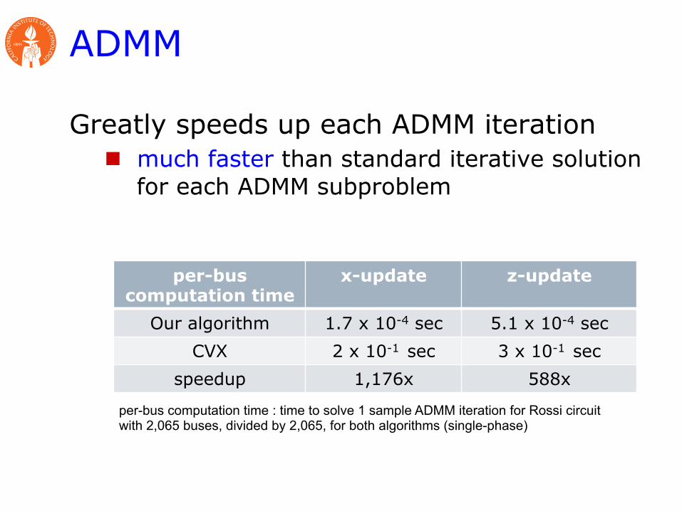
ADMM

Greatly speeds up each ADMM iteration n  much faster than standard iterative solution

for each ADMM subproblem

per-bus computation time

x-update z-update

Our algorithm 1.7 x 10-4 sec 5.1 x 10-4 sec CVX 2 x 10-1 sec 3 x 10-1 sec

speedup 1,176x 588x

per-bus computation time : time to solve 1 sample ADMM iteration for Rossi circuit with 2,065 buses, divided by 2,065, for both algorithms (single-phase)

Challenges Challenges for practical application

n  ADMM too slow for high precision solution n  Relaxation (feasible power flow)

o  Wye loads: empirically exact but no proof o  Delta loads: empirically inexact

n  Offline (distributed) algorithm o  Intermediate iterates are not feasible and cannot be

applied to network

which determines the update of (y1, . . . , y4). In Appendix I,we derive a close form solution for this problem. After thez-update step, we update the Lagrange multipliers for therelaxed constraints as (8c). Both the z-update and multiplierupdate steps only involve local variables of an agent and nocommunication is required.

Finally, we specify the stopping criteria for the algorithm.Empirical results show that the the solution is accurateenough when both the primal residual rk defined in (9a)and the dual residual sk defined in (9b) are below 10

�4pN ,

where N is the number of buses. The pseudo code for thealgorithm is summarized in Table I.

TABLE I: Distributed algorithm of OPF

Distributed Algorithm of OPFInput: network T , power injection region S

i

, voltage region (vi

, v

i

),line impedance z

i

Output: voltage v, power injection s

1. Initialize the variables with any number.2. Iterate the following step until both the primal residual sk (9a) andthe dual residual rk (9b) are below 10�4

pN .

a. In the x-update, each agent i solves (14) to update x.b. In the z-update, each agent i solves (16) to update z.c. In the multiplier update, update �, µ, � by (8c).

IV. CASE STUDY

To demonstrate the scalability of the distributed algorithmproposed in section III, we test it on the model of a 2,065-bus distribution circuit in the service territory of the SouthernCalifornia Edison. There are 1,409 household loads, whosepower consumptions are within 0.07kw–7.6kw and 142 com-mercial loads, whose power consumptions are within 5kw–36.5kw. There are 135 rooftop PV panels, whose nameplatesare within 0.7–4.5kw, distributed across the 1,409 houses.

The network is unbalanced three phase. We assume thatthe three phases are decoupled such that the network be-comes identical single phase network. The voltage magnitudeat each load bus is allowed within [0.95, 1.05] per unit (pu),i.e. v

i

= 1.052 and vi

= 0.952 for i 2 N+. The controldevices are the rooftop PV panels whose real and reactivepower injections are controlled. The objective is to minimizepower loss across the network, namely f

i

(pi

, `i

) = `i

ri

for i 2 N+ in (2). Each bus is an agent and there are2,065 agents in the network that solve the OPF problem ina distributed manner.

The algorithm is implemented in Matlab 2013a and run onMacbook pro 2013 with i5 dual core processor. We mainlyfocus on the following aspects:

• Solution feasibility: the primal residual rk defined in(9a) measures the feasibility of the solution for ADMM[20]. In our algorithm, (12f) are relaxed and rk =p

k(x(1))

k � zkk2 + k(x(2))

k � zkk2 with respect tothe iterations k.

• Optimality: the dual feasibility error sk defined in (9b)measures the optimality of the solution for ADMM [20].In our algorithm, the dual residual sk =

p2⇢kzk �

zk�1k with respect to the iterations k.

(a) Primal and dual residual (b) Objective value

Fig. 4: Simulation results for 2065 bus Rossi circuit.

• Computation time: the proposed distributed algorithmis run on a single machine. We can divide the totaltime by the number of agents to roughly estimatethe time required for each agent if the algorithm isrun on distributed severs (excluding the communicationoverhead).

The stopping criteria is that both the primal and dualresidual are below 10

�4pN and Figure 4a illustrates the

evolution of rk/pN and sk/

pN over iterations k. The

stopping criteria are satisfied after 1, 114 iterations. Theevolution of the objective value is illustrated in Figure 4b.It takes 1,153s to run 1,114 iterations on a single computer.Then the average time spent by each agent is roughly 0.56s(excluding communication overhead) if we implement thealgorithm in a distributed manner.

TABLE II: Statistics of different networks

Network Diameter Iteration Total Time(s) Avg time(s)2065Bus 64 1114 1153 0.561313Bus 53 671 471 0.36792Bus 54 524 226 0.29363Bus 36 289 66 0.18108Bus 16 267 16 0.14

To understand the key factor that affects the convergencerate, we simulate the algorithm on different networks (thatare subnetworks of the 2,065-bus system) and some statisticsare given in Table II. For simplicity, we assume the averagetime T spent by each agent takes the linear form T = ↵N+

�D, where N is network size and D is network diameter.Using the data in Table II, the parameters ↵ = 9.8 ⇥ 10

�7,� = 8.6⇥ 10

�3 give the least square error. This means thatthe convergence rate is mainly determined by the networkdiameter, independent of the network size.

Finally, we show the advantage of deriving close formexpression by comparing the computation time of solvingthe subproblems between off-the-shelf solver (CVX) and ouralgorithm. In particular, we compare the average computationtime of solving the subproblem in both the x-update and thez-update step. In the x-update step, the average time requiredto solve the subproblem is 1.7⇥10

�4s for our algorithm but0.2s for CVX. In the z-update step, the average time requiredto solve the subproblem is 5.1⇥10

�4s for our algorithm but0.3s for CVX. Thus, each ADMM iteration only takes about

Dvijotham (DeepMind)

Realtime AC OPF for tracking

Gan (FB) Tang (Caltech)

Gan & L, JSAC 2016 Tang et al, TSG 2017

See also: Dall’Anese et al, Bernstein et al, Hug & Dorfler et al, Callaway et al

OPF

power flow equations

min c0 (y)+ c(x)over x, ys. t. F(x, y) = 0 y ≤ y x ∈ X := x ≤ x ≤ x{ }

operational constraints

capacity limits controllable devices

uncontrollable state

OPF




capacity limits

OPF




capacity limits

Assume: ∂F∂y

≠ 0 ⇒ y(x) over X

Static OPF

x(t +1) = x(t)−η ∂f∂x

(t)#

$%&

'(Xy(t) = y(x(t))

gradient projection algorithm:

active control

law of physics

min f (x, y(x); µ)over x ∈ X

[Gan & Low, JSAC 2016]

Online (feedback) perspective

Network: power flow solver y(t) : F(x(t), y(t)) = 0

DER : gradient updatex(t+1) = G(x(t), y(t))

control x(t)

measurement, communication

y(t)

physical network

cyber network

•  Explicitly exploits network as power flow solver •  Naturally tracks changing network conditions

Drifting OPF

minx

c0 (y(x))+ c(x)

s. t. y(x) ≤ y x ∈ X

minx

c0 (y(x),γ t )+ c(x,γ t )

s. t. y(x,γ t ) ≤ y x ∈ X

drifting OPF

static OPF

Drifting OPF

min ft (x, y(x); µt )over x ∈ Xt

x(t +1) = x(t) − η H (t)( )−1 ∂ft∂x

(x(t))#

$%&

'(Xty(t) = y(x(t))

active control

law of physics

Quasi-Newton algorithm:

[Tang, Dj & Low, 2017]

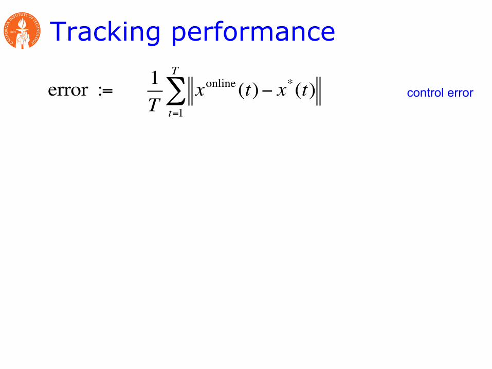
Tracking performance

Theorem

error := 1T

xonline (t)− x*(t)t=1

T

∑

error ≤ λMλm

⋅ε

1−ε⋅

1T

x*(t)− x*(t −1) +Δt( )t=1

T

∑

avg rate of drifting

control error


Theorem

error := 1T


T

∑

error ≤ ελM / λm −ε

⋅1T

x*(t)− x*(t −1) +Δt( )t=1

T

∑ +δ

avg rate of drifting •  of optimal solution •  of feasible injections


Theorem

error := 1T


T

∑


⋅1T

x*(t)− x*(t −1) +Δt( )t=1

T

∑ +δ

error in Hessian approx


Theorem

error := 1T


T

∑


⋅1T

x*(t)− x*(t −1) +Δt( )t=1

T

∑ +δ

“condition number” of Hessian


Theorem

error := 1T


T

∑


⋅1T

x*(t)− x*(t −1) +Δt( )t=1

T

∑ +δ

“initial distance” from x*(t)

Implementation

Implement L-BFGS-B n  More scalable n  Handles (box) constraints X

Simulations n  IEEE 300 bus


IEEE 300 bus

Tracking performance 7

Fig. 3. The absolute and relative gap between the objective values of the real-time operations x(t) and the optimal solutions x

⇤(t).

0.376 sec. We can see that the proposed implementation of thereal-time OPF algorithm is quite computationally efficient.

Fig. 4. Histogram of computation times for each real-time update.

VI. CONCLUSION AND FUTURE DIRECTIONS

In this paper, we proposed a real-time OPF algorithm basedon quasi-Newton methods. This algorithm utilizes real-timemeasurement data and performs suboptimal updates on afaster timescale than traditional OPF. We studied its trackingperformance, and also proposed a specific implementationbased on the L-BFGS-B algorithm. Simulations showed thatthe proposed algorithm can track the optimal operations welland is computationally efficient.

There still remain a number of issues in designing real-time OPF algorithms. Currently the updates are carried outevery 6 seconds, which could be too short for us to neglectthe dynamics for large networks. To extend the time betweeneach updates, we need to improve the algorithm so that it willstill work when larger changes in loads and generations areallowed.

One possible direction is to find more accurate methods ofestimating the Hessian. The L-BFGS-B method turns out to

work well as simulations have shown, but we have also foundsome difficult situations where more accurate estimate of theHessian is needed.

Another possible direction is to introduce dual variablesinstead of penalty functions. It has been observed that byintroducing dual variables, one can usually achieve betterconvergence and smaller constraint violations, and potentiallyavoid numerical issues. We are especially interested in com-bining primal-dual methods with quasi-Newton methods.

Besides improving the tracking performance of the al-gorithm, we are also interested in developing a distributedalgorithm for real-time OPF. As the number of controllabledevices increases, the communication between controllabledevices and the control center will become a bottleneck, anddistributed algorithms will be much favored.

APPENDIX APROOF OF THEOREM 1

We write the box constraint (5c)-(5e) as l(t) x(t) u(t).First we note that, by the definition of �M and �m, we have

kxk2Bt

= x

TBtx �Mx

TWx = �Mkxk2

W

,

kxk2Bt

= x

TBtx � �mx

TWx = �mkxk2

W

,

for any vector x and any t 2 {1, . . . , T}.At the beginning of time t, the initial point is x0(t) =

Ptˆx(t�1), where Pt is the projection onto the current feasiblecontrol region l(t) x(t) u(t), and ˆ

x(t�1) is the previousoperation. Let

mt(x) := g

Tt (x� x0(t))

+

1

2

(x� x0(t))TBt(x� x0(t)).

Then the updated operation ˆ

x(t) is the optimal of

min

l(t)xu(t)mt(x).

IEEE 300 bus

Key message

Large network of DERs n  Real-time optimization at scale n  Computational challenge: power flow solution

Online optimization [feedback control]

n  Network computes power flow solutions in real time at scale for free

n  Exploit it for our optimization/control n  Naturally adapts to evolving network conditions

Examples n  Slow timescale: OPF n  Fast timescale: frequency control

Challenges Challenges for practical application

n  Distributed implementation n  Tracking with lower update speed n  Not all buses have sensors/controllers

Optimal placement dealing with limited sensing/control

Guo (Caltech)

Guo & Low CDC 2017

Summary

Characterization of controllability and observability

n  of swing dynamics n  in terms spectrum of graph Laplacian matrix

Implications on optimal placement of controllable DERs and sensors

n  set covering problem

Network model Pim

i

jPij

di + diswing dynamics:

of buses with controllable loads/sensors. Condition 1) encodesinformation on the graph symmetry and is shown to holdfor almost all practical systems. Condition 2) captures howbuses interact with each other through the network and can beverified using the eigenvectors of the graph Laplacian matrix.We would like to remark that our results do not explicitlyhint on how optimal decentralized control scheme should bedesigned. Indeed, the standard control associated with ourresults is typically centralized and open-loop. The focus ofthis work is more towards a fundamental understanding onstructural properties of such system.

The rest of the paper is organized as follows. We first reviewthe system model and relevant spectral graph theory conceptsin Section II. In Section III, we present the exact conditionsfor the system to be controllable. The practical interpretationsof these conditions are discussed in Section IV. The parallelresults in the system observability are given in Section V. Wepresent two applications of our characterizations in SectionVI. The first application as presented in Section VI-A is moreanalytical, which reduces the problem of optimal placementfor controllable loads and sensors to a set cover problem.The second application as presented in Section VI-B is anevaluation in the IEEE 39-bus New England interconnectiontest system, showing how a single well chosen critical busbased on our theory is capable of regulating the frequency ofthe whole grid. We conclude in Section VII.

II. MODEL AND PROBLEM SETUP

In this section, we present the system model as adoptedin [5]–[8] and review relevant concepts from spectral graphtheory. We also refine the existing models to include thelimited coverage of controllable loads and sensors.

Let R denote the set of real numbers. For a set N , itscardinality is denoted as |N |. We reserve caligraphic symbolslike F ,U ,O for sets related to the physical system (for in-stance buses with controllable loads). Uppercase symbols likeA,B,C usually refer to matrices, but can also refer to a vectorspace or a set in the proofs. For two matrices A,B with properdimensions, [A B] means the concatenation of A,B in a row,and [A;B] means the concatenation of A,B in a column.A variable without subscript usually denotes a vector withappropriate components, e.g., ! = (!

j

, j 2 N ) 2 R|N |. For amatrix A, we denote A

T , A�1, A�1/2 and A

† as its transpose,inverse, inverse of square root and Moore-Penrose pseudo-inverse respectively, provided they are properly defined. Fora time-dependent signal !(t), we use ! to denote its timederivative d!

dt

. For any vector x, we use diag(x) to denote thediagonal matrix with entries from x as the main diagonal.

We use the graph G = (N , E) to describe the powertransmission network, where N = {1, . . . , n} is the set ofbuses and E ⇢ N ⇥N denotes the set of transmission lines.The terms bus/node and line/edge are used interchangeablyin this paper. We assume without loss of generality that G isconnected and simple. An edge in E is denoted either as e or(i, j). We further assign an arbitrary orientation over E so thatif (i, j) 2 E then (j, i) /2 E . For any subset of buses S 2 N ,we denote its characteristic function using the correspondingsymbol 1S . Let n = |N | ,m = |E| be the number of buses

and transmission lines, respectively. The incidence matrix ofG is a n⇥m matrix C defined as

C

ie

=

8><

>:

1 if node i is the source of e�1 if node i is the target of e0 otherwise

For each bus j 2 N , we denote the frequency deviation as!

j

and denote the inertia constant as M

j

> 0. The symbolP

m

j

is overloaded to denote the mechanical power injectionif j is a generator bus and denote the aggregate change inuncontrollable load if j is a load bus. For each transmissionline (i, j) 2 E , we denote as P

ij

the branch flow deviationand denote as B

ij

the link susceptance.At each bus, there are three types of additional components

which affect the system dynamics.1) Controllable Load. Such component incurs extra load

denoted by d

j

and the level of d

j

is controllable. Theset of buses with controllable loads is denoted as U .

2) Frequency Sensitive Load. Such component is sensitiveto local frequency deviations and incurs additional loadof ˆ

d

j

= D

j

!

j

. We do not allow direct control tosuch loads and denote the set of buses with frequencysensitive loads as F .

3) Sensor. Such component measures the local frequencydeviation !

j

. The set of buses equipped with sensors isdenoted as S .

Summarizing the above different components, the swing andnetwork dynamics is given by

�M

j

!

j

= 1F (j) ˆdj + 1U (j)dj � P

m

j

+

X

e2EC

je

P

e

, j 2 N

˙

P

ij

= B

ij

(!

i

� !

j

), (i, j) 2 Eand the system state is observed through

y

j

= 1S(j)!j

, j 2 NReaders are referred to [6] for more detailed justification andderivation of this model.

Now using x to denote the system state x = [!;P ], andputting F , U , S, M , D and B to be the diagonal matriceswith 1F (j), 1U (j), 1S(j), Mj

, Dj

and B

ij

as diagonal entriesrespectively, we can rewrite the system dynamics in the state-space form

x = Ax�M

�1

U

0

�d+

M

�1

0

�P

m (1a)

y =

⇥S 0

⇤x (1b)

whereA =

�M

�1

FD �M

�1

C

BC

T

0

�

and is referred to as the system matrix of (1) in the sequel.In our characterizations, the scaled graph Laplacian matrix

defined as L = M

�1/2

CBC

T

M

�1/2 plays a key role. It ismore explicitly given by

L

ij

=

8><

>:

� BijpMiMj

i 6= j, (i, j) 2 E or (j, i) 2 E1

Mi

Pj:j2N(i)

B

ij

i = j

0 otherwise






j


T , A�1, A�1/2 and A


dt




C

ie

=

8><

>:



j


j

> 0. The symbolP

m

j


ij


ij



denoted by d

j

and the level of d

j



d

j

= D

j

!

j



j



�M

j

!

j

= 1F (j) ˆdj + 1U (j)dj � P

m

j

+

X

e2EC

je

P

e

, j 2 N

˙

P

ij

= B

ij

(!

i

� !

j


y

j

= 1S(j)!j



, Dj

and B

ij


x = Ax�M

�1

U

0

�d+

M

�1

0

�P

m (1a)

y =

⇥S 0

⇤x (1b)

whereA =

�M

�1

FD �M

�1

C

BC

T

0

�


defined as L = M

�1/2

CBC

T

M


L

ij

=

8><

>:

� BijpMiMj

i 6= j, (i, j) 2 E or (j, i) 2 E1

Mi

Pj:j2N(i)

B

ij

i = j

0 otherwise

controllable DER






j


T , A�1, A�1/2 and A


dt




C

ie

=

8><

>:



j


j

> 0. The symbolP

m

j


ij


ij



denoted by d

j

and the level of d

j



d

j

= D

j

!

j



j



�M

j

!

j

= 1F (j) ˆdj + 1U (j)dj � P

m

j

+

X

e2EC

je

P

e

, j 2 N

˙

P

ij

= B

ij

(!

i

� !

j


y

j

= 1S(j)!j



, Dj

and B

ij


x = Ax�M

�1

U

0

�d+

M

�1

0

�P

m (1a)

y =

⇥S 0

⇤x (1b)

whereA =

�M

�1

FD �M

�1

C

BC

T

0

�


defined as L = M

�1/2

CBC

T

M


L

ij

=

8><

>:

� BijpMiMj

i 6= j, (i, j) 2 E or (j, i) 2 E1

Mi

Pj:j2N(i)

B

ij

i = j

0 otherwise

frequency sensor






j


T , A�1, A�1/2 and A


dt




C

ie

=

8><

>:



j


j

> 0. The symbolP

m

j


ij


ij



denoted by d

j

and the level of d

j



d

j

= D

j

!

j



j



�M

j

!

j

= 1F (j) ˆdj + 1U (j)dj � P

m

j

+

X

e2EC

je

P

e

, j 2 N

˙

P

ij

= B

ij

(!

i

� !

j


y

j

= 1S(j)!j



, Dj

and B

ij


x = Ax�M

�1

U

0

�d+

M

�1

0

�P

m (1a)

y =

⇥S 0

⇤x (1b)

whereA =

�M

�1

FD �M

�1

C

BC

T

0

�


defined as L = M

�1/2

CBC

T

M


L

ij

=

8><

>:

� BijpMiMj

i 6= j, (i, j) 2 E or (j, i) 2 E1

Mi

Pj:j2N(i)

B

ij

i = j

0 otherwise

weighted Laplacian matrix

Algebraic coverage

spectral decomposition of L

where N(i) is the set of neighbors of i. For any vector x 2 Rn,we have

x

T

Lx =

X

(i,j)2E

B

ij

x

ipM

i

� x

jpM

j

!2

� 0

This implies that L is a positive semidefinite matrix andthus diagonalizable. It is well-known that rank(L) = n � 1

for a connected graph [16] and therefore 0 is a simpleeigenvalue of L. We denote 0 = �

1

< �

2

· · · �

n

as its eigenvalues and put � := {�1

,�

2

, · · · ,�n

} to be anorthonormal set of its eigenvectors with �

s

affording �

s

. Thenotation N = {1, 2, . . . , n} is abused to also denote the indexset of �. Whether N denotes the set of buses or denotes anindex set for � will be clear from the context. The followingproperty of the spectrum of L turns out to be particularlyuseful in this work.

Definition II.1. The matrix L is said to have simple spectrumif all the eigenvalues of L are distinct.

We recommend the readers to take M = I

n

and B = I

m

infirst reading, under which our results are significantly cleaneryet all key points (except Proposition IV.1) are captured.Throughout the analysis, we make the following assumption:

Sensitive Load Frequency sensitive components only existat buses with controllable loads. That is, we assume F ⇢ U .

III. CONTROLLABILITY

In this section, we analyze the state-space dynamics givenin (1) and characterize its controllability using the spectra ofthe scaled Laplacian matrix L.

Before presenting our characterization, we first clarify whatwe mean by the controllability of (1). The classical definitionof controllability requires the whole state space Rn+m beingreachable from any initial point. This turns out to be too strongand is not suitable for our application. Indeed, from the branchflow dynamics

˙

P = BC

T

!

we see that

B

�1

(P (t)� P (0)) =

Zt

0

C

T

!(s)ds 2 range(C

T

)

If we assume the system is in the nominal state at time t = 0,then we know B

�1

P (t) 2 range(C

T

) for any t. In otherwords, the scaled branch flow vector is confined in the rangeof C

T because of the system physics. This motivates thefollowing definition.

Definition III.1. The dynamics (1) is said to be P-controllableor controllable in power system sense, if for any t > 0, initialstate x(0) = [!(0);P (0)] and target state x(t) = [!(t);P (t)]

satisfying

B

�1

(P (t)� P (0)) 2 range(C

T

)

there exists a control u such that

x(t) = �(x(0), u, t)

where �(x(0), u, t) is the system state at time t given initialstate x(0) and control input u.

Our first result generalizes the classical Kalman criteria tothe context of P-controllability. It shows that to determine thesystem P-controllability, it suffices to form the controllabilitymatrix with the scaled Laplacian matrix L (instead of the fullsystem matrix A) and we can ignore the drifting term P

m

(even when it is time-variant) in (1a).

Proposition III.2. The dynamics (1) is P-controllable if andonly if the matrix

W =

⇥M

�1/2

U �LM

�1/2

U · · · (�L)

n�1

M

�1/2

U

⇤

has full row rank.

The proof of this proposition is presented in Appendix A.This result tells us that to decide the P-controllability of (1),it amounts to compute the rank of W . Recall 0 = �

1

< �

2

· · · �

n

are the eigenvalues of L and {�1

,�

2

, . . . ,�

n

} isan orthonormal set of corresponding eigenvectors. Let Q bethe matrix with �

j

’s as columns and ⇤ be the diagonal matrixwith �

j

’s as diagonal entries, i.e. L = Q⇤Q

T . To facilitate thediscussion, we introduce the concept of algebraic coverage.

Definition III.3. With all previous notations, the algebraiccoverage of a bus j 2 N , denoted as cov(j), is defined to bethe set

cov(j) := {s 2 N : �

s,j

6= 0}where �

s,j

is the j-th entry of �s

.

Now we are ready to give the spectral characterization forthe P-controllability of (1).

Theorem III.4. With all the previous notations, the dynamics(1) is P-controllable if and only if

1) The scaled Laplacian matrix L has simple spectrum2) The algebraic coverage from controllable loads is full

N =

[

j2Ucov(j) (2)

Proof. Recall U is the diagonal matrix encoding the placementof controllable loads. Let V be the Vandermonde matrix

V =

2

6664

1 ��

1

�

2

1

· · · (��

1

)

n�1

1 ��

2

�

2

2

· · · (��

2

)

n�1

......

.... . .

...1 ��

n

�

2

n

· · · (��

n

)

n�1

3

7775

andu

j

= Q

T

M

�1/2

U

j

, 8j 2 Nwhere U

j

is the j-th column of U .Since Q is orthogonal, we know (�L)

k

= Q(�⇤)

k

Q

T andas a result

W = Q

⇥Q

T

M

�1/2

U · · · (�⇤)

n�1

Q

T

M

�1/2

U

⇤(3)

For any integer p, q, we denote as r(p, q) the unique numberr 2 {1, 2, · · · , q} such that p = qk + r for some integer k.Define a permutation matrix ⇧ 2 Rn

2⇥n

2

given by

⇧

ij

=

(1 j = (r(i, n)� 1)n+ b(i� 1)/nc+ 1

0 otherwise

eigenvectors of L

Q = β1 ! βn[ ]

algebraic coverage of bus j

cov( j) := s βsj ≠ 0{ }

Controllability

∪j∈U

cov( j) = all buses{ }

Theorem Swing dynamics is controllable if and only if n  L has a simple spectrum n  controllable DERs have full coverage

holds a.s.

Observability

∪j∈S

cov( j) = all buses{ }

Theorem Swing dynamics is observable if and only if n  L has a simple spectrum n  frequency sensors have full coverage

holds a.s.

Application

Optimal placement of DER & frequency sensors

n  set covering problem n  always install sensors at buses with

controllable DERs, and vice versa

Application

Fig. 2. Line diagram of the IEEE 39-bus New England interconnection testsystem.

Corollary VI.1. For the dynamics (1), the set of optimalplacements of controllable loads and the set of optimal place-ment of sensors are the same.

This result tells us that, in practice, we should always installsensors to the buses with controllable loads, and vice versa.

B. Secondary frequency regulation with a single bus

We now demonstrate how our results can identify criticalbuses for controllability by evaluating over the IEEE 39-busNew England interconnection test system, as shown in Fig. 2.There are 10 generators and 29 load nodes in the system, andin contrast to our linearized model for theoretical study, thesimulation adopts more realistic nonlinear dynamics.

One can check that the L matrix associated with thisnetwork has simple spectrum (which is as expected accordingto Proposition IV.1) and that the bus 35 has full algebraiccoverage, i.e. all the eigenvectors �

s

of L have nonzero entryat position 35. Therefore Theorem III.4 implies that evenif we can only inject control at bus 35, the system is stillP-controllable. Thus we should be able to drive the wholesystem back to the nominal state after arbitrary disturbance.In order to verify this, we add a step increase of 1 pu tothe generation at bus 30, and compare the system evolutionwith or without control at bus 35. In contrast to the standardcontrol associated with the controllability Gramian, the controlwe adopt here utilizes only local frequency deviation. Detailsabout the control scheme design can be found in [24]. Thesimulation results are shown in Fig. 3.

As one can see from the figure, despite the geograph-ical distance between the disturbance and the controllablenode, the control scheme successfully drives the grid backto nominal state within 5 seconds. In contrast, when nocontrol is posed, the bus frequencies still stabilize becauseof governor dynamics, but not to the nominal state. Moreover,the stabilization process takes considerably longer time. Suchdifference demonstrates that with a single bus 35 chosen basedon our theory, frequency regulation over the grid can actuallybe achieved.

(a) With control. (b) Without control.

Fig. 3. Comparison of the system evolution with and without control at bus35 after adding a step increase of 1 pu to the generation at bus 30.

VII. CONCLUSION

In this work, we develop full characterizations on theimpact of limited controllable loads/sensors coverage overthe controllability/observability for the swing and power flowdynamics in frequency regulation. We present two applicationsof our theoretical results: 1) an analytical application whichreduces the problem of optimal placement of controllable loadsand sensors to a set cover problem; 2) an evaluation over theIEEE 39-bus New England interconnection test system wheresecondary frequency control over the whole network can beachieved by a single critical bus chosen based on our theory.

Our results can be extended in several directions. First,the linearized model (1) is usually accurate near the nominaloperation point, but may incur noticeable error when thesystem is far away from the equilibrium. Such scenariosmay arise after a system failure. It is thus interesting to seehow our results can be generalized to nonlinear dynamics.Second, the control suggested by our result can be verycostly. It is of interest to understand what the cheapest controlshould be if we already know the system is controllable, andhow the placement of controllable loads affects this optimalcost. Third, in applications, we usually only focus on thecontrollability over a subset of transmission lines that aresubject to congestion. We should understand whether we canrefine the theory so that the results can be tailored for suchpartial controllability.

ACKNOWLEDGEMENT

The authors would like to thank Professor Janusz Bialekfrom Skoltech, John Pang and Chen Liang from Caltech forhelpful discussions. This work has been supported by NSFgrants through EPCN 1619352, CNS 1545096 CCF 1637598,ARPA-E grant through award DE-AR0000699 and DTRAthrough grant HDTRA 1-15-1-0003.

REFERENCES

[1] B. J. Kirby, “Spinning reserve from responsive loads,” Report of OakRidge National Laboratory, 2003.

[2] PNNL, “Grid friendly controller helps balance energy supply anddemand.” [Online]. Available: http://readthis.pnl.gov/MarketSource/ReadThis/B3099 not print quality.pdf

[3] D. Trudnowski, M. Donnelly, and E. Lightner, “Power-system frequencyand stability control using decentralized intelligent loads,” in 2005/2006IEEE/PES Transmission and Distribution Conference and Exhibition,May 2006, pp. 1453–1459.

[4] N. Lu and D. J. Hammerstrom, “Design considerations for frequencyresponsive grid friendlytm appliances,” in 2005/2006 IEEE/PES Trans-mission and Distribution Conference and Exhibition, May 2006, pp.647–652.

IEEE 39-bus New England system

1pu step disturbance at bus 30 Fig. 2. Line diagram of the IEEE 39-bus New England interconnection testsystem.






s





VII. CONCLUSION



ACKNOWLEDGEMENT


REFERENCES





without control

Fig. 2. Line diagram of the IEEE 39-bus New England interconnection testsystem.






s





VII. CONCLUSION



ACKNOWLEDGEMENT


REFERENCES





with local control at single bus 35

nominal frequency restored

Outline

Relaxations of AC OPF n  Dealing with nonconvexity

Distributed AC OPF n  Dealing with scalability

Realtime AC OPF n  Dealing with volatility

Optimal placement n  Dealing with limited sensing/control

autonomous energy grid optimization - nrel.gov · pdf filesteven low nrel, september 2017 ....

Documents