autonomous landing of a quadcopter on a high-speed … · autonomous landing of a quadcopter on a...
TRANSCRIPT

Autonomous Landing of a Quadcopter
on a High-Speed Ground Vehicle
Alexandre Borowczyk1, Duc-Tien Nguyen2, André Phu-Van Nguyen3,
Dang Quang Nguyen4, David Saussié5, and Jerome Le Ny6
Polytechnique Montreal and GERAD, Montreal, QC H3T 1J4, Canada
I. Introduction
The ability of multirotor micro aerial vehicles (MAVs) to perform stationary hover flight makes
them particularly interesting for a variety of applications, e.g., site surveillance, parcel delivery, or
search and rescue operations. At the same time however, they are challenging to use on their own
because of their relatively short battery life and range. Deploying and recovering MAVs from mobile
Ground Vehicles (GVs) could alleviate this issue and allow more efficient deployment and recovery
in the field. For example, delivery trucks, public buses or marine carriers could be used to transport
MAVs between locations of interest and allow them to recharge periodically [1, 2]. For search and
rescue operations, the synergy between ground and air vehicles could help save precious mission
time and would pave the way for the efficient deployment of large fleets of autonomous MAVs.
The idea of better integrating GVs and MAVs has indeed already attracted the attention of
multiple car and MAV manufacturers [3, 4]. Research groups have previously considered the problem
of landing a MAV on a mobile platform, but most of the existing work is concerned with landing
on a marine platform or with precision landing on a static or slowly moving ground target. In
[5] for example, a custom visual marker made of concentric rings allows relative pose estimation
between the GV and the MAV, and MAV control is performed using optical flow measurements
1 System Software Specialist, [email protected] Ph.D candidate, Electrical Engineering Department, [email protected], AIAA Student Member.3 M.Sc. student, Electrical Engineering Department, [email protected] M.Sc. student, Electrical Engineering Department, [email protected] Assistant Professor, Department of Electrical Engineering, [email protected], AIAA Member.6 Assistant Professor, Department of Electrical Engineering, [email protected], AIAA Senior Member.
1

and velocity commands. More recently, [6] used the ArUco library from [7] as a visual fiducial and
IMU measurements fused in a square-root unscented Kalman filter for relative pose estimation. The
system however still relies on optical flow for accurate velocity estimation. This becomes problematic
as soon as the MAV aligns itself with a moving ground platform, at which point the optical flow
camera suddenly measures the velocity of MAV relative to the platform instead of the velocity
relative to the ground frame. Muskardin et al. [8] developed a system to land a fixed wing MAV
on top of a moving GV. However, their approach requires that the GV cooperates with the MAV
during the landing maneuver and makes use of expensive RTK-GPS units. Kim et al. [9] land a
MAV on a moving target using simple color blob detection and a non-linear Kalman filter, but test
their solution only for speeds of less than 1 m/s. Most notably, Ling [10] shows that it is possible to
use low cost sensors combined with an AprilTag fiducial marker [11] to land on a small ground robot.
He further demonstrates different methods to help accelerate the AprilTag detection. He notes in
particular that as a quadcopter pitches forward to follow the ground platform, the downward facing
camera frequently loses track of the visual target, which stresses the importance of a model-based
estimator such as a Kalman filter to compensate.
The references above address the terminal landing phase of the MAV on a moving platform,
but a complete system must also include a strategy to guide the MAV towards the GV during
its approach phase. Proportional Navigation (PN) [12, Chapter 5] is most commonly known as a
guidance law for ballistic missiles, but can also be used for UAV guidance. Indeed, [13] describes a
form of PN tailored to road following by a fixed-wing vehicle, using visual feedback from a gimbaled
camera. Gautam et al. [14] compare pure pursuit, line-of-sight and PN guidance laws to conclude
that PN is the most efficient in terms of the total required acceleration and the time necessary to
reach the target. On the other hand, within close range of the target, PN becomes inefficient. To
alleviate this problem, [15] proposes to switch from PN to a proportional-derivative (PD) controller.
Finally, to maximize the likelihood of a smooth transition from PN to PD, [16] proposes to point a
gimbaled camera towards the target.
Contributions and organization of the paper. This note describes a complete system allowing a
multirotor MAV to land autonomously on a ground platform moving at relatively high speed, using
2
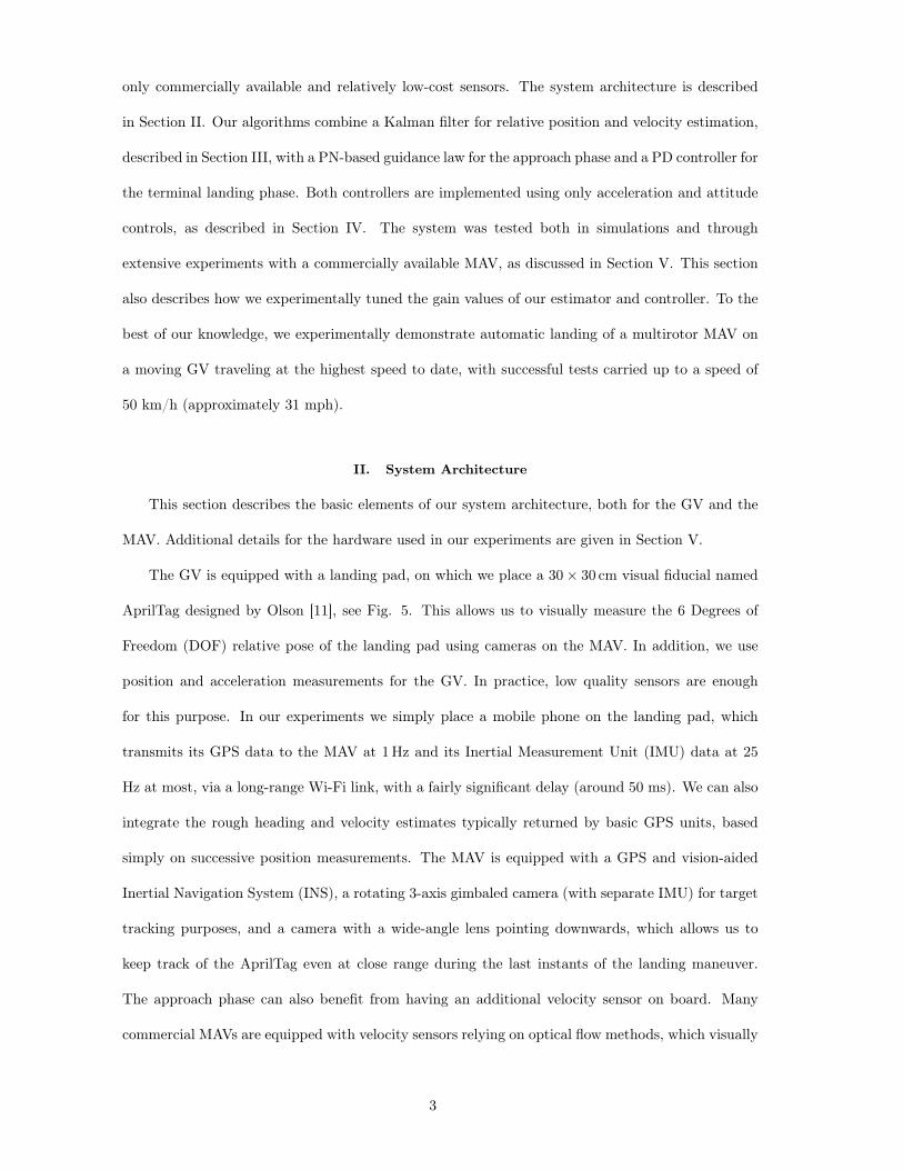
only commercially available and relatively low-cost sensors. The system architecture is described
in Section II. Our algorithms combine a Kalman filter for relative position and velocity estimation,
described in Section III, with a PN-based guidance law for the approach phase and a PD controller for
the terminal landing phase. Both controllers are implemented using only acceleration and attitude
controls, as described in Section IV. The system was tested both in simulations and through
extensive experiments with a commercially available MAV, as discussed in Section V. This section
also describes how we experimentally tuned the gain values of our estimator and controller. To the
best of our knowledge, we experimentally demonstrate automatic landing of a multirotor MAV on
a moving GV traveling at the highest speed to date, with successful tests carried up to a speed of
50 km/h (approximately 31 mph).
II. System Architecture
This section describes the basic elements of our system architecture, both for the GV and the
MAV. Additional details for the hardware used in our experiments are given in Section V.
The GV is equipped with a landing pad, on which we place a 30× 30 cm visual fiducial named
AprilTag designed by Olson [11], see Fig. 5. This allows us to visually measure the 6 Degrees of
Freedom (DOF) relative pose of the landing pad using cameras on the MAV. In addition, we use
position and acceleration measurements for the GV. In practice, low quality sensors are enough
for this purpose. In our experiments we simply place a mobile phone on the landing pad, which
transmits its GPS data to the MAV at 1 Hz and its Inertial Measurement Unit (IMU) data at 25
Hz at most, via a long-range Wi-Fi link, with a fairly significant delay (around 50 ms). We can also
integrate the rough heading and velocity estimates typically returned by basic GPS units, based
simply on successive position measurements. The MAV is equipped with a GPS and vision-aided
Inertial Navigation System (INS), a rotating 3-axis gimbaled camera (with separate IMU) for target
tracking purposes, and a camera with a wide-angle lens pointing downwards, which allows us to
keep track of the AprilTag even at close range during the last instants of the landing maneuver.
The approach phase can also benefit from having an additional velocity sensor on board. Many
commercial MAVs are equipped with velocity sensors relying on optical flow methods, which visually
3

estimate velocity by computing the movement of features in successive images, see, e.g., [17].
Four main coordinate frames are defined and illustrated in Fig. 1. The global North-East-
Down (NED) frame, denoted N, is located at the first point detected by the MAV. Assuming for
concreteness that the MAV is a quadcopter, the body frame B is chosen according to the cross
“×” configuration, i.e., its forward x-axis points between two of the arms and its y-axis points to the
right. The frame for the downward facing rigid camera is obtained from B by a rotation around
the zB axis, which is perpendicular to the image plane of the camera. Finally, the gimbaled camera
frame G is attached to the lens center of the moving camera. Its forward z-axis is perpendicular
to the image plane and its x-axis points to the right of the gimbal frame.
NxN
yN
zN
zB
Horizontal plane
zGxG
yG
AprilTag
GGimbaled camera
xB
Global NED
B
M1
M2
M3
M4
yB
Quadrotor
Fig. 1 Frames of reference used.
III. Kalman filter
Estimation of the position, velocity and acceleration of the MAV and the landing pad, as
required by our guidance and control system, is performed by a Kalman filter [18] running on the
MAV. The Kalman filter algorithm follows the standard two steps, with the prediction step running
at 100 Hz and update steps executed for each sensor individually as soon as new measurements
become available. The architecture of this filter is shown in Fig. 2 and its parameters are described
in the following paragraphs.
4
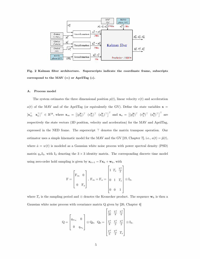
Fig. 2 Kalman filter architecture. Superscripts indicate the coordinate frame, subscripts
correspond to the MAV (m) or AprilTag (a).
A. Process model
The system estimates the three dimensional position p(t), linear velocity v(t) and acceleration
a(t) of the MAV and of the AprilTag (or equivalently the GV). Define the state variables x =
[x>m x>a ]> ∈ R18, where xm =[(pNm)> (vNm)> (aNm)>
]> and xa =[(pNa )> (vNa )> (aNa )>
]> are
respectively the state vectors (3D position, velocity and acceleration) for the MAV and AprilTag,
expressed in the NED frame. The superscript > denotes the matrix transpose operation. Our
estimator uses a simple kinematic model for the MAV and the GV [19, Chapter 7], i.e., a(t) = p(t),
where a = w(t) is modeled as a Gaussian white noise process with power spectral density (PSD)
matrix qwI3, with I3 denoting the 3 × 3 identity matrix. The corresponding discrete time model
using zero-order hold sampling is given by xk+1 = Fxk + wk, with
F =
Fm 0
0 Fa
, Fm = Fa =
1 TsT 2s
2
0 1 Ts
0 0 1
⊗ I3,
where Ts is the sampling period and ⊗ denotes the Kronecker product. The sequence wk is then a
Gaussian white noise process with covariance matrix Q given by [20, Chapter 4]
Q =
qwm0
0 qwa
⊗Q0, Q0 =
T 5s
20T 4s
8T 3s
6
T 4s
8T 3s
3T 2s
2
T 3s
6T 2s
2 Ts
⊗ I3,
5

where the parameters qwmand qwa
for the PSD of the MAV and GV acceleration are set by an
empirical tuning process (qwm = 3.0 m2/s5 and qwa = 3.25 m2/s5 in our experiments).
B. Measurement Models
Different types of measurements are integrated independently through Kalman filter update
steps at different rates following Fig. 2. Each measurement vector zk is assumed to follow a model
zk = Hkxk + vk, (1)
where vk is a Gaussian white noise with covariance matrices Vk, uncorrelated from the process noise
wk. The following subsections detail the matrices Hk and Vk for each type of measurements.
1. MAV position, velocity and acceleration from the Integrated Navigation System
The integrated navigation system of our MAV combines IMU, GPS and visual measurements
to provide us with position, velocity and gravity compensated acceleration data directly expressed
in the global NED frame, so Hk =
[I9 09×9
]for these measurements. However, the velocity
measurements relying on optical flow methods are not correct when the MAV flies above a moving
platform. We empirically found that increasing the standard deviation of the velocity measurement
noise from 0.1 m/s in the approach phase to 10 m/s in the landing phase allowed us to mostly
discount these measurements when flying close to the GV.
2. GPS measurements for the GV
The GPS unit of the mobile phone on the GV’s landing pad provides measurements of its latitude
la, longitude lo (both in radians), altitude al, speed Ua and heading ψa. This information is sent to
the MAV’s on-board computer via a wireless link. The landing pad’s position pNa =
[xNa yNa zNa
]>in the global NED frame is then computed as xNa ≈ (la − la0)RE , yNa ≈ (lo − lo0) cos(la)RE ,
zNa = al0 − al, where RE = 6378137 m is the Earth radius, and the subscripts 0 correspond to
the starting point. These relations are valid over sufficiently short travel distances and under a
spherical Earth assumption, but more precise transformations could be used [21, Chapter 2]. The
horizontal components of the current velocity vNa of the GV in the global NED frame are calculated
6
as xNa = Ua cos(ψa), yNa = Ua sin(ψa). Hence, for the model (1) the quantities xNa , yNa , zNa , xNa ,
yNa are measured and Hk =
[05×9 I5 05×4
]. However, because the GPS velocity and heading
measurements have poor accuracy at low speed, we discard them if Ua < 2.5 m/s, in which case
only xNa , yNa , zNa are measured and Hk =
[03×9 I3 03×6
].
Our GPS receiver provides an estimate of the noise standard deviation for the measurements
xNa and yNa . The noise on the measurements zNa , xNa and yNa is heuristically assumed independent,
with standard deviations set empirically for zNa to the same value as for xNa , yNa , and to 0.25 m/s
for xNa , yNa in our experiments. We use a low-cost GPS unit with output rate of about 1 Hz. This
source of data is only used to approach the GV but is insufficient for landing on it. For the landing
phase, we use the gimbaled and bottom facing cameras to detect the AprilTag.
3. Gimbaled Camera measurements
The gimbaled camera together with the AprilTag detection algorithm provides measurements
pGm/a in frame G of the relative position between the MAV and the AprilTag, with centimeter
accuracy, at range up to 5 m. This information is converted into the global NED frame N by
computing pNm − pNa = RNG p
Gm/a, where RN
G is the rotation matrix from N to G returned by the
gimbal IMU. Therefore, for the observation model (1) the quantities xNm−xNa , yNm−yNa , and zNm− zNa
are measured and Hk =
[I3 03×6 −I3 03×6
]. Here the standard deviation of the measurement
noise is empirically set to 0.2 m. To reduce the chances of target loss, the gimbaled camera centers
the image onto the AprilTag as soon as visual detection is achieved. When the AprilTag cannot be
detected, we follow the control scheme proposed by [16] to point the camera towards the landing
pad using the estimated line-of-sight (LOS) information obtained from the Kalman filter.
4. Bottom camera measurements
The downward facing camera is used to assist the last moments of the landing, when the MAV
is close to the landing pad, yet too far to cut off the motors. At that moment, the gimbaled camera
cannot perceive the whole AprilTag but a fixed, wide angle camera can still provide measurements.
This camera measures the target’s position in its own frame C, which is obtained from frame B
by a simple rigid transformation. The observation model is the same as for the gimbaled camera
7
except for the transformation to the global NED frame, i.e., pNm − pNa = RNC p
Cm/a where RN
C denotes
the rotation matrix from N to C provided by the MAV INS. We set the noise standard deviation
empirically to 0.3 m. Note that this is higher than for the gimbaled camera noise because of the
greater distortion introduced by the wide-angle lens, especially on the edges of the image.
5. Landing pad acceleration using the mobile phone’s IMU
Finally, since most mobile phones also contain an IMU, we leverage this sensor to estimate
the GV’s acceleration. For the observation model (1), the quantities xNa , yNa , zNa are measured
(again, after gravity compensation by the internal IMU algorithms) and Hk =
[03×15 I3
]. In our
experiments we set the standard deviation of these measurements on all 3 axes to 0.6 m/s2.
The output of the Kalman filter is the input to the guidance and control system described in
the next section, which is used by the MAV to approach and land safely on the moving platform.
IV. Guidance and Control System
For GV tracking by the MAV, we use a guidance strategy switching between a Proportional
Navigation (PN) law [12, Chapter 5] for the approach phase and a PD controller for the landing
phase, which is similar in spirit to the approach in [15]. The approach phase is characterized by
a large distance between the MAV and the GV and the absence of visual data to localize the GV.
Hence, in this phase, the MAV can only rely on the data transmitted by the GV’s GPS and IMU. The
goal of the controller is then to follow an efficient “pursuit” trajectory, which is achieved here by a
PN controller augmented with a closing velocity controller and the MAV flying at constant altitude.
In contrast, the landing phase is characterized by a relatively close proximity between the MAV and
the GV, and the availability of visual feedback to determine the AprilTag’s relative position. This
phase requires a higher level of accuracy and faster response time from the controller, and a PD
controller can be more easily tuned to meet these requirements than a PN controller. In addition,
the system should transition from one controller to the other seamlessly, avoiding discontinuity in
the commands sent to the MAV.
8

A. Proportional Navigation Guidance
The PN guidance law [12, Chapter 5] uses the fact that two vehicles are on a collision course if
the orientation of their LOS vector remains constant. It aims at keeping the rotation of the velocity
vector of the MAV proportional to the rotation of the LOS vector. Hence, our PN controller provides
an acceleration command that is normal to the instantaneous LOS vector
a⊥ = −λ|u| u|u|× Ω, with Ω =
u× uu · u
, (2)
where λ is a gain parameter, u = pNa − pNm and u = vNa − vNm are (estimates) obtained from the
Kalman filter and represent the LOS vector and its derivative expressed in the NED frame, and Ω
is the rotation vector of the LOS.
We then supplement the PN guidance law (2) with an approach velocity controller determining
the acceleration a‖ along the LOS direction, which in particular allows us to specify a high enough
velocity required to properly overtake the target. This acceleration component is computed using
the PD structure a‖ = Kp‖u+Kd‖ u, where Kp‖ and Kd‖ are constant gains. The total acceleration
command is obtained by combining both components as a = a⊥ + a‖. Since only the horizontal
control is of interest, the acceleration along z-axis is disregarded.
The desired acceleration is then converted to attitude control inputs that are more compatible
with the MAV input format. In frame N, the quadcopter dynamic equations of translation read
as follows [22, Chapter 2]
maNm =
0
0
mg
+ RNB
0
0
−T
+ FD
where T is the total thrust created by the rotors, FD the drag force, m the MAV mass, g the
standard gravity constant, and RNB denotes the rotation matrix from N to B given by
RNB =
cθcψ sφsθcψ − cφsψ cφsθcψ + sφsψ
cθsψ sφsθsψ + cφcψ cφsθsψ − sφcψ
−sθ sφcθ cφcθ
,
with the notation cx = cosx and sx = sinx. The angles φ, θ, and ψ denote roll, pitch and yaw,
9
respectively. We get
m
xm
ym
zm
=
0
0
mg
−cφsθcψ + sφsψ
cφsθsψ − sφcψ
cφcθ
T − kdxm|xm|
ym|ym|
zm|zm|
,
where the drag is roughly modeled as a force proportional to the signed quadratic velocity in each
direction and kd is a constant, which we estimated by recording the terminal velocity for a range of
attitude controls at level flight and performing a least squares regression on the data. For constant
flight altitude, T = mg/cφcθ and assuming ψ = 0, it yields
m
xmym
= mg
− tan θ
tanφ/ cos θ
− kdxm|xm|ym|ym|
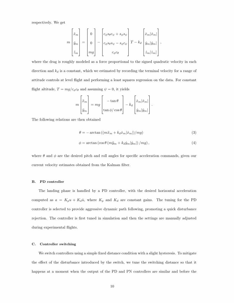
.The following relations are then obtained
θ = − arctan ((mxm + kdxm|xm|)/mg) (3)
φ = arctan (cos θ (mym + kdym|ym|) /mg) , (4)
where θ and φ are the desired pitch and roll angles for specific acceleration commands, given our
current velocity estimates obtained from the Kalman filter.
B. PD controller
The landing phase is handled by a PD controller, with the desired horizontal acceleration
computed as a = Kpu + Kdu, where Kp and Kd are constant gains. The tuning for the PD
controller is selected to provide aggressive dynamic path following, promoting a quick disturbance
rejection. The controller is first tuned in simulation and then the settings are manually adjusted
during experimental flights.
C. Controller switching
We switch controllers using a simple fixed distance condition with a slight hysteresis. To mitigate
the effect of the disturbance introduced by the switch, we tune the switching distance so that it
happens at a moment when the output of the PD and PN controllers are similar and before the
10
visual target acquisition. This last point ensures that the switch does not disturb the tracking of
the AprilTag. Through a series of experiments we set the switching distance to 6 m.
D. Vertical control
The entire approach phase is done at a constant altitude, which is handled by the internal
vertical position controller of the MAV. The descent is initiated once the quadrotor has stabilized
over the landing platform. A constant vertical velocity command is then issued to the MAV and
maintained until it reaches a height of 0.2 m above the landing platform, at which point the motors
are disarmed.
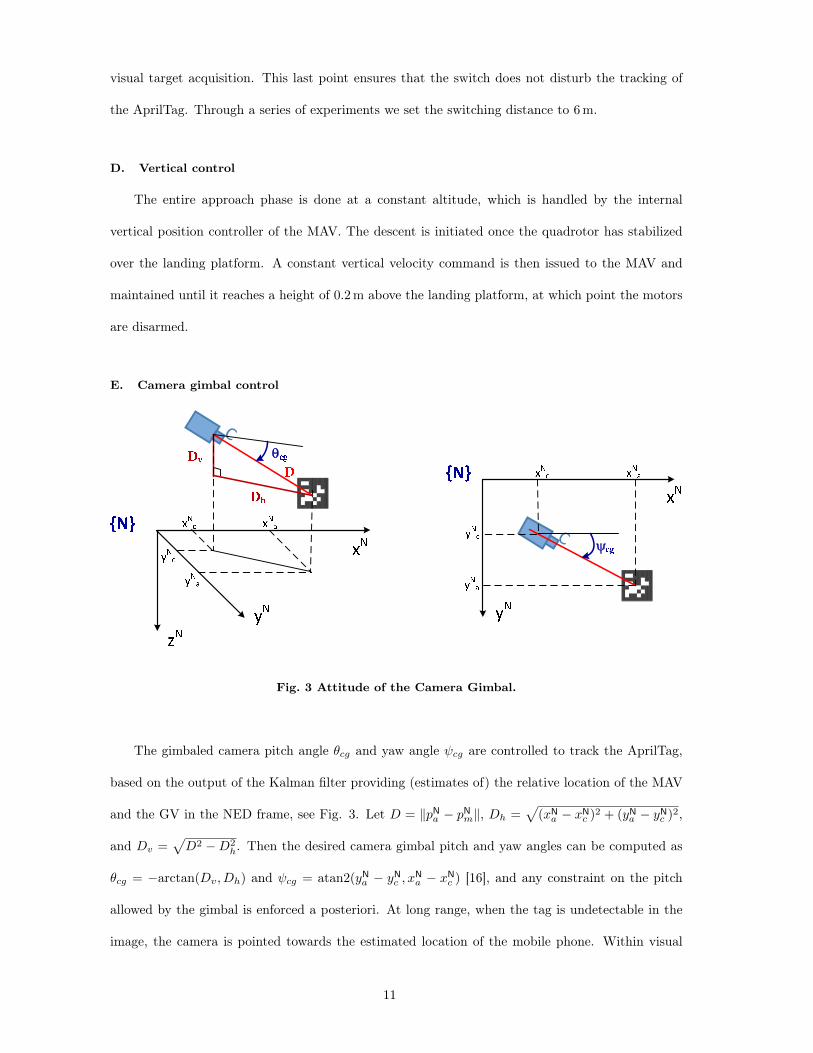
E. Camera gimbal control
Fig. 3 Attitude of the Camera Gimbal.
The gimbaled camera pitch angle θcg and yaw angle ψcg are controlled to track the AprilTag,
based on the output of the Kalman filter providing (estimates of) the relative location of the MAV
and the GV in the NED frame, see Fig. 3. Let D = ‖pNa − pNm‖, Dh =√
(xNa − xNc )2 + (yNa − yNc )2,
and Dv =√D2 −D2
h. Then the desired camera gimbal pitch and yaw angles can be computed as
θcg = −arctan(Dv, Dh) and ψcg = atan2(yNa − yNc , xNa − xNc ) [16], and any constraint on the pitch
allowed by the gimbal is enforced a posteriori. At long range, when the tag is undetectable in the
image, the camera is pointed towards the estimated location of the mobile phone. Within visual
11

range, the camera is positioned so that the AprilTag is centered in the image.
V. Experimental Validation
A. System Description
We implemented our system on a commercial off-the-shelf DJI Matrice 100 (M100) quadcopter
shown in Fig. 4. All computations are performed on the standard on-board computer of this
platform (DJI Manifold), which contains an Nvidia Tegra K1 SoC. The 3-axis gimbaled camera is a
Zenmuse X3, from which we receive 720p YUV color images at 30 Hz. To reduce computations, we
drop the U and V channels and downsample the images to obtain 640 × 360 monochrome images.
We modified the M100 to rigidly attach a downward facing Matrix Vision mvBlueFOX camera,
equipped with an ultra-wide angle Sunex DSL224D lens with a diagonal field of view of 176 degrees.
The M100 is also equipped with the DJI Guidance module, which includes one additional downward
facing camera for optical flow measurements and seamlessly integrates with the INS to provide us
with position, velocity and acceleration measurements of the M100 using a fusion of on-board sensors
described in [17]. This information is used as input to our Kalman filter, see Section III B 1.
Fig. 4 The M100 quadcopter. Note that all side facing cameras of the Guidance module were
removed and the down facing BlueFox camera sits behind the bottom Guidance sensor.
Our algorithms were implemented in C++ using ROS (Robot Operating System) [23]. They rely
on an open source implementation of the AprilTag library [11] based on OpenCV. With accelerations
provided by OpenCV4Tegra, we can run the tag detection at a full 30 frames-per-second (fps) using
12

the X3 camera and at 20 fps with the BlueFOX camera. As mentioned in Section IV, we implemented
our control system using pure attitude control in the xy axes and velocity control in the z axis. The
reason for not using velocity controls is that the internal velocity estimator of the M100 relies on
optical flow measurements from the Guidance system, but the nature of these measurements changes
drastically once the quadcopter starts flying over the landing platform. Although optical flow could
be used to measure the relative velocity of the car, it is difficult to accurately detect the moment
where flow measurements transition from being with respect to the ground to being with respect to
the moving car.
B. Tuning of Kalman Filter Gains
The most arduous step of implementing our system is the tuning of the noise covariance values
associated with each source of information integrated into the Kalman Filter. We first perform
simple experiments to gather baseline data from the mobile phone, e.g., walking and running in
a straight line or walking in a square pattern. We then tune the noise parameters of the mobile
phone data (IMU, GPS position, GPS speed and heading) until the filter satisfactorily estimates the
executed trajectory. Once these parameters are set, we perform baseline flight experiments where
we gather data from the MAV’s integrated navigation system in addition to the mobile phone’s
data. Flight tests include landing on a static target, following the landing pad without landing and
landing on a dynamic target. At first, we exclude the data of our vision sensors, keeping the state
estimation of the landing pad and MAV independent. We then tune the gains related to the INS
data until the filter outputs data closely reflecting our flight tests. We also review the tuning of
noise parameters of the mobile phone data.
The next step is to tune the gains related to our vision sensors, i.e., the AprilTag detection by the
gimbaled and fixed cameras. Since the experimental setup for this step does not require much space,
it is possible to use a motion capture system to compare the output of the filter to ground truth
data. The experimental setup consists of raising the MAV on two rails above an AprilTag. Data
from the gimbal camera and the bottom facing camera are gathered while the AprilTag is moved at
various positions under the MAV. The Kalman filter parameters of the camera measurements are
13

then tuned by using the motion capture data as a guideline.
The final step in tuning our filter is to globally adjust our parameters. Using all the data from
flight experiments, we evaluated the tuning of the Kalman filter as a whole. The goal is to tune
the weights attributed to the mobile phone data, the MAV navigation system and the camera data
with respect to each other.
C. Tuning of Controller Gains
Preliminary tuning of the controller is first performed in DJI’s proprietary simulator and final
adjustments are performed during experimental outdoor tests. Simulating both the approach and
landing phases allows us to determine approximate values for the proportional gain of the PN
controller, the proportional and derivative gains of the PD controller, and the controller switching
distance. The numerical value of the proportional gain for the PN is usually between 3 and 5. Using
the simulator, we validate that the time response is acceptable and that the requested commands
are within the MAV’s capabilities. Flight tests then allow us to confirm that the MAV behaves as
in the simulation, and to test the controller’s performance in windy conditions.
D. Experimental Results
Fig. 5 Experimental setup showing the required equipment on the car. In practice the mobile
phone could also be held inside the car as long as GPS signals are received.
First we demonstrate the validity of our PN controller for the long range approach with a person
running in an approximate straight line, and the MAV chasing him without any visual feedback.
Fig. 6 shows that the MAV converges to the person’s position, in this case after about 7 s. The
speed estimation is not particularly accurate and is only corrected at 1Hz. However this is good
14
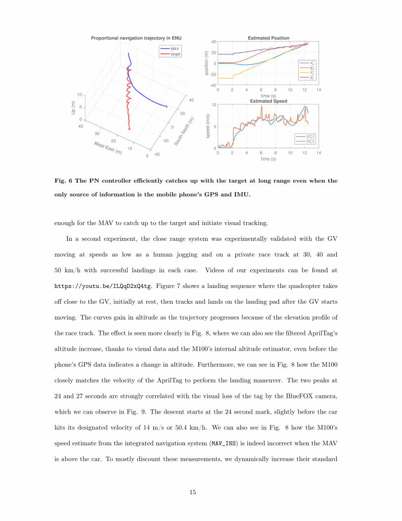
Fig. 6 The PN controller efficiently catches up with the target at long range even when the
only source of information is the mobile phone’s GPS and IMU.
enough for the MAV to catch up to the target and initiate visual tracking.
In a second experiment, the close range system was experimentally validated with the GV
moving at speeds as low as a human jogging and on a private race track at 30, 40 and
50 km/h with successful landings in each case. Videos of our experiments can be found at
https://youtu.be/ILQqD2xQ4tg. Figure 7 shows a landing sequence where the quadcopter takes
off close to the GV, initially at rest, then tracks and lands on the landing pad after the GV starts
moving. The curves gain in altitude as the trajectory progresses because of the elevation profile of
the race track. The effect is seen more clearly in Fig. 8, where we can also see the filtered AprilTag’s
altitude increase, thanks to visual data and the M100’s internal altitude estimator, even before the
phone’s GPS data indicates a change in altitude. Furthermore, we can see in Fig. 8 how the M100
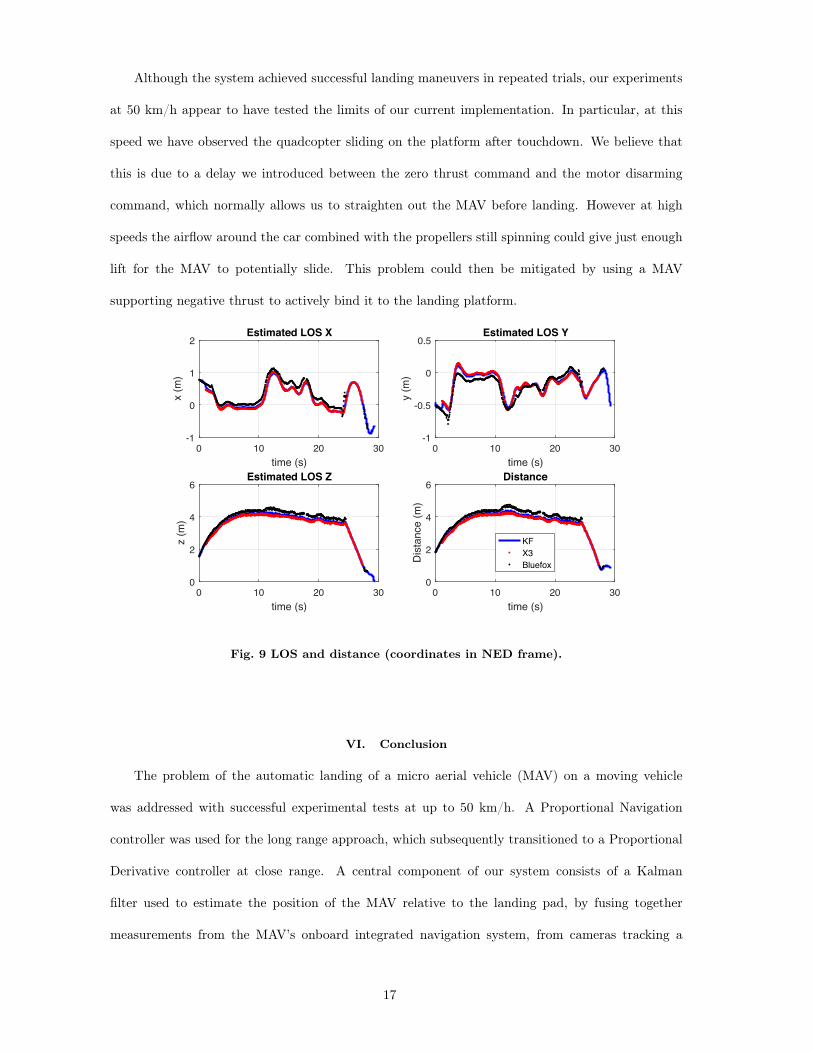
closely matches the velocity of the AprilTag to perform the landing maneuver. The two peaks at
24 and 27 seconds are strongly correlated with the visual loss of the tag by the BlueFOX camera,
which we can observe in Fig. 9. The descent starts at the 24 second mark, slightly before the car
hits its designated velocity of 14 m/s or 50.4 km/h. We can also see in Fig. 8 how the M100’s
speed estimate from the integrated navigation system (MAV_INS) is indeed incorrect when the MAV
is above the car. To mostly discount these measurements, we dynamically increase their standard
15
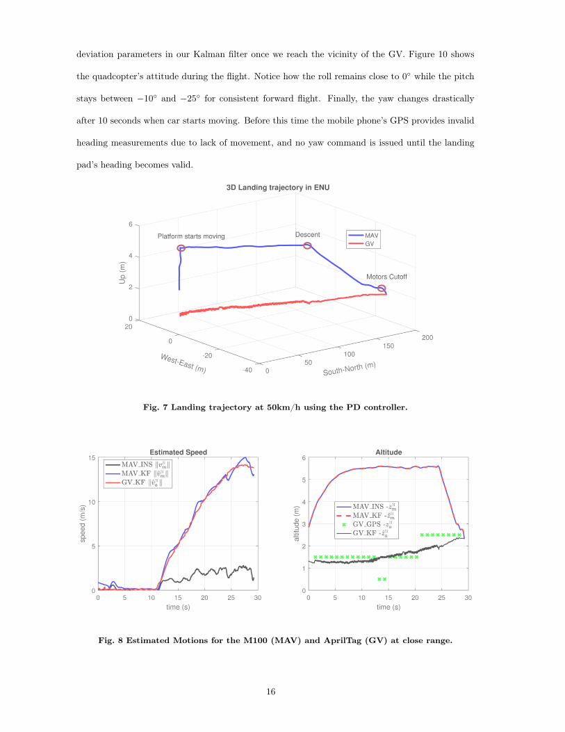
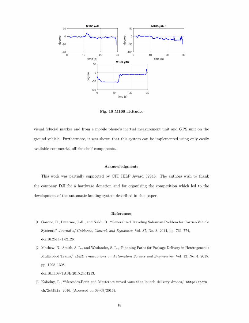
deviation parameters in our Kalman filter once we reach the vicinity of the GV. Figure 10 shows
the quadcopter’s attitude during the flight. Notice how the roll remains close to 0 while the pitch
stays between −10 and −25 for consistent forward flight. Finally, the yaw changes drastically
after 10 seconds when car starts moving. Before this time the mobile phone’s GPS provides invalid
heading measurements due to lack of movement, and no yaw command is issued until the landing
pad’s heading becomes valid.
Fig. 7 Landing trajectory at 50km/h using the PD controller.
Fig. 8 Estimated Motions for the M100 (MAV) and AprilTag (GV) at close range.
16
Although the system achieved successful landing maneuvers in repeated trials, our experiments
at 50 km/h appear to have tested the limits of our current implementation. In particular, at this
speed we have observed the quadcopter sliding on the platform after touchdown. We believe that
this is due to a delay we introduced between the zero thrust command and the motor disarming
command, which normally allows us to straighten out the MAV before landing. However at high
speeds the airflow around the car combined with the propellers still spinning could give just enough
lift for the MAV to potentially slide. This problem could then be mitigated by using a MAV
supporting negative thrust to actively bind it to the landing platform.
0 10 20 30time (s)
-1
0
1
2
x (m
)
Estimated LOS X
0 10 20 30time (s)
-1
-0.5
0
0.5
y (m
)
Estimated LOS Y
0 10 20 30time (s)
0
2
4
6
z (m
)
Estimated LOS Z
0 10 20 30time (s)
0
2
4
6
Dis
tanc
e (m
)
Distance
KFX3Bluefox
Fig. 9 LOS and distance (coordinates in NED frame).
VI. Conclusion
The problem of the automatic landing of a micro aerial vehicle (MAV) on a moving vehicle
was addressed with successful experimental tests at up to 50 km/h. A Proportional Navigation
controller was used for the long range approach, which subsequently transitioned to a Proportional
Derivative controller at close range. A central component of our system consists of a Kalman
filter used to estimate the position of the MAV relative to the landing pad, by fusing together
measurements from the MAV’s onboard integrated navigation system, from cameras tracking a
17
0 10 20 30
time (s)
-40
-20
0
20
degre
e
M100 roll
0 10 20 30
time (s)
-100
-50
0
50
degre
e
M100 pitch
0 10 20 30
time (s)
-100
-50
0
50
degre
e
M100 yaw
Fig. 10 M100 attitude.
visual fiducial marker and from a mobile phone’s inertial measurement unit and GPS unit on the
ground vehicle. Furthermore, it was shown that this system can be implemented using only easily
available commercial off-the-shelf components.
Acknowledgments
This work was partially supported by CFI JELF Award 32848. The authors wish to thank
the company DJI for a hardware donation and for organizing the competition which led to the
development of the automatic landing system described in this paper.
References
[1] Garone, E., Determe, J.-F., and Naldi, R., “Generalized Traveling Salesman Problem for Carrier-Vehicle
Systems,” Journal of Guidance, Control, and Dynamics, Vol. 37, No. 3, 2014, pp. 766–774,
doi:10.2514/1.62126.
[2] Mathew, N., Smith, S. L., and Waslander, S. L., “Planning Paths for Package Delivery in Heterogeneous
Multirobot Teams,” IEEE Transactions on Automation Science and Engineering, Vol. 12, No. 4, 2015,
pp. 1298–1308,
doi:10.1109/TASE.2015.2461213.
[3] Kolodny, L., “Mercedes-Benz and Matternet unveil vans that launch delivery drones,” http://tcrn.
ch/2c48his, 2016. (Accessed on 09/09/2016).
18
[4] Lardinois, F., “Ford And DJI Launch $100,000 Developer Challenge To Improve Drone-To-Vehicle
Communications,” tcrn.ch/1O7uOFF, 2016. (Accessed on 09/28/2016).
[5] Lange, S., Sunderhauf, N., and Protzel, P., “A vision based onboard approach for landing and posi-
tion control of an autonomous multirotor UAV in GPS-denied environments,” in “Proceedings of the
International Conference on Advanced Robotics (ICAR),” Munich, Germany, 2009, pp. 1–6.
[6] Yang, S., Ying, J., Lu, Y., and Li, Z., “Precise quadrotor autonomous landing with SRUKF vision per-
ception,” in “Proceedings of the IEEE International Conference on Robotics and Automation (ICRA),”
Seattle, Washington, 2015, pp. 2196–2201,
doi:10.1109/ICRA.2015.7139489.
[7] Garrido-Jurado, S., Muñoz-Salinas, R., Madrid-Cuevas, F., and Marín-Jiménez, M., “Automatic gen-
eration and detection of highly reliable fiducial markers under occlusion,” Pattern Recognition, Vol. 47,
No. 6, 2014, pp. 2280 – 2292,
doi:10.1016/j.patcog.2014.01.005.
[8] Muskardin, T., Balmer, G., Wlach, S., Kondak, K., Laiacker, M., and Ollero, A., “Landing of a fixed-
wing UAV on a mobile ground vehicle,” in “Proceedings of the IEEE International Conference on
Robotics and Automation (ICRA),” Stockholm, Sweden, 2016, pp. 1237–1242,
doi:10.1109/ICRA.2016.7487254.
[9] Kim, J., Jung, Y., Lee, D., and Shim, D. H., “Outdoor autonomous landing on a moving platform
for quadrotors using an omnidirectional camera,” in “Proceedings of the International Conference on
Unmanned Aircraft Systems (ICUAS),” Orlando, Florida, 2014, pp. 1243–1252,
doi:10.1109/ICUAS.2014.6842381.
[10] Ling, K., Precision Landing of a Quadrotor UAV on a Moving Target Using Low-cost Sensors, Master’s
thesis, University of Waterloo, 2014.
[11] Olson, E., “AprilTag: A robust and flexible visual fiducial system,” in “Proceedings of the IEEE Inter-
national Conference on Robotics and Automation,” Shanghai, China, 2011, pp. 3400–3407,
doi:10.1109/ICRA.2011.5979561.
[12] Kabamba, P. T. and Girard, A. R., Fundamentals of Aerospace Navigation and Guidance, Cambridge
Aerospace Series, Cambridge University Press, 2014. Chapter 5.
[13] Holt, R. and Beard, R., “Vision-based road-following using proportional navigation,” Journal of Intel-
ligent and Robotic Systems, Vol. 57, No. 1-4, 2010, pp. 193 – 216,
doi:10.1007/s10846-009-9353-7.
[14] Gautam, A., Sujit, P. B., and Saripalli, S., “Application of guidance laws to quadrotor landing,” in
19
“Proceedings of the International Conference on Unmanned Aircraft Systems (ICUAS),” Denver, Col-
orado, 2015, pp. 372–379,
doi:10.1109/ICUAS.2015.7152312.
[15] Tan, R. and Kumar, M., “Tracking of ground mobile targets by quadrotor unmanned aerial vehicles,”
Unmanned Systems, Vol. 2, No. 02, 2014, pp. 157–173,
doi:10.1142/S2301385014500101.
[16] Lin, C. E. and Yang, S. K., “Camera gimbal tracking from UAV flight control,” in “Proceedings of the
International Automatic Control Conference (CACS),” Kaohsiung, Taiwan, 2014, pp. 319–322,
doi:10.1109/CACS.2014.7097209.
[17] Zhou, G., Fang, L., Tang, K., Zhang, H., Wang, K., and Yang, K., “Guidance: A visual sensing
platform for robotic applications,” in “Proceedings of the IEEE Conference on Computer Vision and
Pattern Recognition Workshops (CVPRW),” Boston, Massachusetts, 2015, pp. 9–14,
doi:10.1109/CVPRW.2015.7301360.
[18] Kalman, R. E., “A New Approach to Linear Filtering and Prediction Problems,” Transactions of the
ASME–Journal of Basic Engineering, Vol. 82, No. Series D, 1960, pp. 35–45.
[19] Farrell, J., Aided Navigation: GPS with High Rate Sensors, McGraw-Hill, Inc., New York, NY, USA,
1st ed., 2008. Chapter 7.
[20] Zarchan, P. and Musoff, H., Fundamentals of Kalman Filtering: A Practical Approach, American
Institute of Aeronautics and Astronautics, Incorporated, 2000. Chapter 4.
[21] Groves, P. D., Principles of GNSS, inertial, and multisensor integrated navigation systems, GNSS/GPS
Series, Artech House, 2nd ed., 2013. Chapter 2.
[22] Stevens, B., Lewis, F., and Johnson, E., Aircraft Control and Simulation: Dynamics, Controls Design,
and Autonomous Systems, Wiley, 2015. Chapter 2.
[23] Quigley, M., Conley, K., Gerkey, B. P., Faust, J., Foote, T., Leibs, J., Wheeler, R., and Ng, A. Y.,
“ROS: an open-source Robot Operating System,” in “Proceedings of the ICRA Workshop on Open
Source Software,” Vol. 3, 2009, p. 5.
20