avessel noise budget for admiralty inlet, puget sound...

A vessel noise budget for Admiralty Inlet, Puget Sound,Washington (USA)

Christopher Bassetta) and Brian PolagyeDepartment of Mechanical Engineering, University of Washington, Seattle, Stevens Way, Box 352600,Seattle, Washington 98165

Marla HoltConservation Biology Division, Northwest Fisheries Science Center, National Marine Fisheries Service,National Oceanic and Atmospheric Administration, 2725 Montlake Boulevard East, Seattle, Washington98112

Jim ThomsonApplied Physics Laboratory, University of Washington, Seattle, 1013 Northeast 40th Street, Box 355640,Seattle, Washington 98105-6698

(Received 18 March 2012; revised 3 August 2012; accepted 28 September 2012)

One calendar year of Automatic Identification System (AIS) ship-traffic data was paired with

hydrophone recordings to assess ambient noise in northern Admiralty Inlet, Puget Sound, WA

(USA) and to quantify the contribution of vessel traffic. The study region included inland waters

of the Salish Sea within a 20 km radius of the hydrophone deployment site. Spectra and hourly,

daily, and monthly ambient noise statistics for unweighted broadband (0.02–30 kHz) and marine

mammal, or M-weighted, sound pressure levels showed variability driven largely by vessel traffic.

Over the calendar year, 1363 unique AIS transmitting vessels were recorded, with at least one AIS

transmitting vessel present in the study area 90% of the time. A vessel noise budget was

calculated for all vessels equipped with AIS transponders. Cargo ships were the largest contributor

to the vessel noise budget, followed by tugs and passenger vessels. A simple model to predict

received levels at the site based on an incoherent summation of noise from different vessels

resulted in a cumulative probability density function of broadband sound pressure levels that

shows good agreement with 85% of the temporal data. VC 2012 Acoustical Society of America.

[http://dx.doi.org/10.1121/1.4763548]

PACS number(s): 43.30.Nb, 43.50.Lj, 43.50.Cb, 43.50.Rq [AMT] Pages: 3706–3719

I. INTRODUCTION

The impacts of high energy, impulsive sources of

anthropogenic sounds such as sonars and seismic exploration

on marine species have been an area of active research

(NRC, 2000, 2003). Increasingly, concerns have expanded to

include continuous, lower energy sources such as shipping

traffic. Low-frequency ambient noise levels in the open

ocean have long been attributed to maritime traffic (Wenz,

1962; Urick, 1967; Ross, 1976; Greene and Moore, 1995;

McDonald et al., 2006; McDonald et al., 2008; Hildebrand,

2009; Frisk, 2012). Low-frequency (<500 Hz), high energy

(>180 dB re 1 lPa at 1 m) noise generated by large shipping

vessels propagates efficiently across ocean basins, contribut-

ing to ambient noise levels over large distances (>100 km).

At shorter distances (<10 km), higher frequency noise may

also be significant (NRC, 2003).

The acoustic signature (i.e., spectral characteristics) of a

vessel depends on its design characteristics (e.g., gross ton-

nage, draft), on-board equipment (e.g., generators, engines,

active acoustics equipment), and operating conditions (e.g.,

speed, sea state) (Ross, 1976). The primary sound generation

mechanism for commercial vessels is cavitation, which pro-

duces broadband noise and tonal components related to the

rotation rate of the ship propeller (Gray and Greeley, 1980).

Source levels for vessels, referenced to dB re 1 lPa at 1 m,

range from 150 dB for small fishing vessels and recreational

watercraft to 195 dB for super tankers (Gray and Greeley,

1980; Kipple and Gabriele, 2003; Hildebrand, 2005). Peaks

in spectral levels for shipping traffic occur at frequencies

less than 500 Hz with substantial tonal contributions as low

as 10 Hz (Ross, 1976; Scrimger and Heitmeyer, 1991;

Greene and Moore, 1995). Small ships are quieter at low fre-

quencies but can approach or exceed noise levels of larger

ships at higher frequencies (Greene and Moore, 1995; Kipple

and Gabriele, 2003; Hildebrand, 2005). Radiated noise levels

are also directional and vary based on vessel orientation or

aspect (Arveson and Vendittis, 2000; Trevorrow et al.,2008). In addition to mechanical noise, active acoustics devi-

ces are a significant high-frequency noise source due to the

widespread use of fish finding and depth sounding devices

(NRC, 2005). Source levels for common active acoustics

devices are on the order of 150–200 dB at frequencies from

3 to 200 kHz, with the most common commercial devices

operating above 50 kHz (NRC, 2003; Hildebrand, 2004).

However, downward directionality and rapid attenuation at

high frequencies limit their contribution to broadband noise

levels over large spatial scales.

a)Author to whom correspondence should be addressed. Electronic mail:

[email protected]

3706 J. Acoust. Soc. Am. 132 (6), December 2012 0001-4966/2012/132(6)/3706/14/$30.00 VC 2012 Acoustical Society of America

Downloaded 11 Dec 2012 to 128.208.234.149. Redistribution subject to ASA license or copyright; see http://asadl.org/terms

mailto:[email protected]

To understand the effects noise may have on marine

mammal populations, the frequency content of different

noise sources should be evaluated because mammalian hear-

ing is not uniformly sensitive to all frequencies and different

species have different hearing ranges. On the basis of avail-

able audiograms, Southall et al. (2007) proposes a weighting

function or “M-weighting” for five groups of marine mam-

mals based on functional hearing ranges to better quantify

sound exposure for predicting auditory injury and other ex-

posure effects in these animals. The five functional hearing

groups are low-frequency cetaceans (baleen whales), mid-

frequency cetaceans (toothed whales and most oceanic dol-

phins), high-frequency cetaceans (porpoises, river dolphins,

and other small cetaceans), pinnipeds (seals, seal lions, and

walruses) in water, and pinnipeds in air. Southall et al. note

that these weighting functions are precautionary and, in

some cases, are likely to overestimate the sensitivity of indi-

viduals. The four functional hearing groups relevant to this

study are low-frequency cetaceans, mid-frequency ceta-

ceans, high-frequency cetaceans, and pinnipeds in water.

Noise budgets quantify the relative contributions of dif-

ferent sources to ambient noise levels. Ambient noise is typi-

cally defined as the background noise attributed to natural

physical processes and, increasingly, anthropogenic sources

(Dahl et al., 2007). Some definitions exclude identifiable

sources such as individual vessels (NRC, 2003). Because

vessel traffic is ubiquitous in busy coastal areas, the former

definition (including individual vessels) is adopted for this

study. In the case of shipping traffic, the National Research

Council suggests identifying the contributions of unique ves-

sel types over different temporal and spatial scales (NRC,

2003; Southall, 2005). Such information is needed to assess

the impact of vessel noise on marine mammals in coastal

waters, which often serve as critical habitat. Hatch et al.(2008) undertook a study of vessel noise and estimated a

vessel noise budget for the Stellwagen Bank National

Marine Sanctuary (SBNMS) to better understand the effect

this noise might have on endangered North Atlantic right

whales (Eubalaena glacialis). A similar methodology is

applied to develop a vessel noise budget for Admiralty Inlet,

Puget Sound, WA (Fig. 1). This study varies from Hatch

et al. (2008) in that it considers frequencies up to 30 kHz

rather than an upper limit of 1 kHz. Furthermore, this study

treats anthropogenic noise in a biologically specific manner

by comparing M-weighted statistics to unweighted broad-

band noise statistics.

II. STUDY SITE

The site consists of contiguous waters within a 20 km ra-

dius of a point 700 m to the southwest of Admiralty Head.

The area serves as important habitat for a number of marine

species. Specifically, Admiralty Inlet is designated as critical

habitat for Southern Resident killer whales (Orcinus orca)

(NMFS, 2006) and is regularly used by a number of other

marine mammal species, including gray whales (Eschrich-tius robustus), harbor porpoise (Phocoena phocoena), and

Steller sea lions (Eumetopias jubatus). It is also an important

migratory corridor for several fishes, including endangered

salmonids. Admiralty Inlet is the primary inlet to Puget

Sound, separating the Main Basin from the Strait of Juan de

Fuca, and is 5 km wide at its narrowest point. The passage

provides shipping access to the ports of Seattle, Everett, and

Tacoma, as well as a number of U.S. Navy and Coast Guard

facilities (e.g., Puget Sound Naval Shipyard, Bangor Sub-

marine Base). Passenger ferries, serving as a transportation

link between coastal communities, and cruise ships also

make regular transits in the study area.

This research provides context for understanding exist-

ing underwater noise levels in Puget Sound and what poten-

tial further increases could result from additional

development of the region’s coastal waters. Particularly, Ad-

miralty Inlet is a candidate for tidal energy development and

potential impacts to marine species are under consideration.

Information about the contribution of vessel traffic to the

noise budget can inform the assessment of potential acoustic

effects of tidal turbine installation, operations, and

maintenance.

Van Parijs et al. (2009) note that the descriptive spatial

scales, typically used in atmospheric sciences and oceanog-

raphy, can be applied to studies of ecology. With respect to

acoustics, the scales can be related to the distances over

which species vocally communicate with conspecifics. The

study area encompasses 562 km2 of the Salish Sea, and, in

accordance with the spatial scales outlined by Orlanski

(1975), constitutes a mesoscale vessel noise budget.

III. METHODS

A. Acoustics data

Autonomous hydrophones positioned 1 m above the

seabed were used to collect acoustic data. The hydrophones

were deployed on a fixed tripod at a depth of approximately

FIG. 1. (Color online) (a) The Salish

Sea with the study area highlighted.

(b) Admiralty Inlet bathymetry and

deployment site (closed circle) with

extent of ship tracking (white out-

line). (c). Ship tracks from January 1

to January 15, 2011. Gray lines are

local ferry traffic and black lines are

all other vessel traffic.

J. Acoust. Soc. Am., Vol. 132, No. 6, December 2012 Bassett et al.: Admiralty Inlet vessel noise budget 3707


60 m. All deployments were within 45 m of the coordinates

48.1530�N, 122.6882�W. The acoustic recording system

consisted of a self-contained data acquisition and storage

system (Loggerhead Instruments DSG, Sarasota, FL) with a

hydrophone (HTI-96-Min) and internal preamplifier. The

hydrophone had an effective sensitivity of �166 dB re

lPa V�1. Digitized 16 bit data were written to a Secure Digi-

tal (SD) card. For ambient noise analysis, data were obtained

during four deployments of three months duration (from May

7, 2010 to May 9, 2011). The sampling frequency was 80 kHz

on a 1% duty cycle (7 s continuous recording every 10 min).

A shorter deployment (from February 10 to February 21,

2011), sampled at 80 kHz on a 17% duty cycle (10 s at top of

each minute), was used to estimate acoustic source levels for

different vessel types. Data from all deployments were

analyzed from 20 Hz to 30 kHz. Throughout this document,

decibels are referenced to 1 lPa.

Each recording was post-processed into windows con-

taining 65 536 (216) data points with a 50% overlap. Win-

dows were detrended, weighted by a Hann function, and a

fast Fourier transform was applied. Resulting spectra were

then scaled to preserve total variance. Variable frequency-

band merging was applied on a decadal basis to produce

smooth, well-resolved spectra with high confidence. The fre-

quencies, number of merged bands, resulting bandwidth, and

the equivalent degrees of freedom of the spectra are included

in Table I.

Daily, hourly, and monthly statistics for unweighted

broadband sound pressure levels (0.02–30 kHz) and

M-weighted levels were calculated using hydrophone record-

ings collected between May 7, 2010 and May 1, 2011. For

each calculation, recordings were split into subsets represent-

ing the statistical value of interest. For example, statistics for

the hour of 01:00 to 02:00 were calculated by identifying all

recordings taken between these hours over the course of the

year. The mean representing the hour from 01:00 to 02:00

was obtained by averaging all recordings included in that

subset. For all temporal statistics, M-weighted values for the

four marine mammal functional groups (low-, mid-, and

high-frequency cetaceans; pinnipeds in water) were also

calculated. Temporal statistics were calculated in local time

to account for daily patterns associated with scheduled

vessel traffic (e.g., ferries operate on local time).

Cumulative probability distribution functions were cal-

culated by binning unweighted and M-weighted broadband

sound pressure levels. The distributions were obtained by

defining discrete sound pressure level bins, identifying the

number of weighted and unweighted recordings below

the defined upper threshold for each bin, and normalizing the

results by the total number of recordings in the analysis. The

cumulative probability distribution functions highlight the

overall temporal distribution of noise level statistics. A

modeled cumulative probability distribution of unweighted

broadband sound pressure levels was compared with the

measured distribution.

B. Current measurements

Peak tidal currents in northern Admiralty Inlet exceed

3.0 m s�1 (Thomson et al., 2012). When strong currents flow

over the hydrophone, the turbulent pressure fluctuations are

recorded by the hydrophone as additional noise. These pres-

sure fluctuations, often referred to as pseudosound or flow-

noise, are non-propagating and are of sufficient intensity to

mask propagating noise sources including large ships (Lee

et al., 2011). Because pseudosound is non-propagating, it

should not be included in the noise budget. In addition, when

depth-averaged currents exceed 1 m s�1, noise levels

increase with current at frequencies greater than 2 kHz.

These increases are consistent with the mobilization of

gravel, small cobbles, and shell hash (Thorne et al., 1984;

Thorne, 1990).

Acoustic recordings with depth-averaged currents

exceeding 0.4 m s�1 were excluded from this analysis to pre-

vent biasing the statistics with pseudosound, which also

excludes propagating ambient noise from bedload transport.

These periods were identified using co-spatial velocity

records from an Acoustic Doppler Current Profiler (470 kHz

Nortek Continental, Nortek AS, Vangkroken, Norway). Cur-

rent profiles were calculated in 1 m bins using 10 min ensem-

ble averages.

To verify that excluding periods with strong currents

from analysis was not likely to bias statistics related to

vessel noise, an average vessel presence was calculated in

0.1 m s�1 velocity bins for all current data. In each bin, a

summation of all recorded vessel minutes was normalized by

the total number of minutes during which currents in each

bin were recorded. The results were compared to justify the

assumption that vessel presence was independent of currents.

C. Automatic Identification System data

Automatic Identification System (AIS) transponders are

used as a real-time collision avoidance tool and are man-

dated for commercial maritime vessels exceeding 300 gross

tons, tugs and tows, and passenger ships (Federal Register,

2003). Although not required, some recreational vessels are

also equipped with the AIS transponders. AIS transponders

transmit very high frequency radio signals, referred to here

as AIS strings, containing dynamic ship information (i.e.,

position, heading, course over ground, and speed over

ground) up to twice per second while a vessel is in transit.

Static information, including but not limited to ship name,

type, length overall, draft and destination are transmitted ev-

ery 6 min while in transit. A unique Maritime Mobile Serv-

ice Identity (MMSI) number is transmitted with both static

and dynamic data.

AIS transmissions were logged by a receiver (Comar

AIS-2-USB, Comar Systems Ltd., Cowes, UK) on the Admi-

ralty Head Lighthouse at Fort Casey State Park, WA,

approximately 1 km from the hydrophone deployment site.

TABLE I. Merged frequency bands.

Frequency (kHz) 0.01–0.1 0.1–1 1–10 10–30

Merged bands 0 3 19 41

Df (Hz) 1.2 3.7 23.2 50.0

Degrees of freedom 10 30 190 410

3708 J. Acoust. Soc. Am., Vol. 132, No. 6, December 2012 Bassett et al.: Admiralty Inlet vessel noise budget


The receiver was connected to a data acquisition computer

running a PYTHON script to record all incoming AIS strings

and append time stamps. In post-processing, a PYTHON pack-

age (NOAA data version 0.43) (Schwehr, 2010) converted

all received AIS transmissions into an array of text data for

further manipulation. For each received AIS string with

dynamic data, the MMSI number, speed over ground, course

over ground, and vessel coordinates were stored. Static infor-

mation including the vessel length overall, vessel name, and

vessel type were recorded in a look-up table containing in-

formation about all vessels recorded in the study area.

The vessel coordinates from the processed AIS strings

containing dynamic ship information were used to calculate

a radial distance between the ship and the hydrophone (given

a water depth of approximately 60 m, the radial distance and

slant distance were nearly equivalent for most transmis-

sions). Dynamic AIS information for each vessel in the study

area at any time was averaged over 1 min periods. Data were

filtered to include only those AIS transmissions from vessels

under way (speed over ground greater than 0.1 kn) within the

geographic area outlined in Fig. 1. Transmission/receipt

of implausible local coordinates (latitude > 90�, longitude

> 180�) occurred infrequently and has been noted in other

studies (e.g., Harati-Mokhtari et al., 2007).

Records of MMSI numbers, ship types, and ship lengths

were compared against online public information. Using ves-

sel names, information was found by searching a registered

vessel database in the United States or other available online

fleet information.1 To the greatest extent possible, unknown

and incorrect ship types were corrected to accurate values,

unrealistic speeds over ground removed, incorrect ship

lengths updated, and records with invalid MMSI numbers

excluded through manual analysis.

The vessels were separated into four broad categories,

as defined by their AIS vessel codes—“commercial” (AIS

codes 70-89, 30-32, 52), “passenger” (60-69), “other” (90-

99), and “various” (all other codes). Within the commercial

category, vessels were further separated by AIS vessel code

into cargo ships (AIS code 70-79), tankers (80-89), tugs (31,

32, 52), and fishing vessels (30). The cargo category was

subdivided into four different vessel types, using their

MMSI numbers, emphasizing differences in vessel design

related to the type of transported good. The four cargo types

include container vessels, vehicle carriers, general cargo ves-

sels, and bulk carriers. The cargo type for each vessel was

determined by cross-checking the vessel name with available

fleet information. Throughout the rest of the document,

references to cargo vessels include the four types within this

category unless otherwise noted.

Within the passenger category, vessels were separated

by MMSI into local passenger ferries, cruise ships, and

“passenger other” for vessels that do not fit into the first two

passenger vessel designations. As for cargo vessels, this cat-

egorization was motivated by the presence of vessels with

the same AIS vessel code, but different design characteris-

tics. For example, a small whale-watching vessel (length

overall <20 m) and a cruise ship both used AIS code 60

while their expected source levels varied significantly. The

category “various” was used to combine uncommon ship

types (e.g., underwater operations vessels and anti-pollution

equipment) and ship types underrepresented by AIS statistics

(e.g., military vessels and pleasure craft). The vessel code

“other,” an AIS designation, was used by vessels that have

no formal designation that fits within another class (e.g.,

research vessels).

The average and standard deviations of the speed over

ground and length overall were determined for each type.

These metrics were calculated directly from all 1 min aver-

aged data associated with each type. By this method, slow

moving vessels contributed more points to the statistics,

potentially biasing the statistics toward the speeds and

lengths of the slower vessels. However, the statistics calcu-

lated using this method were similar, within 3 kn of speed

over ground and 10% of the length overall, to distance-

weighted statistics for all vessel types but ferries. For ferries,

the statistics were different due to a distribution dominated

by a set of small, faster moving ferries and a larger, slower

moving ferry.

To visualize vessel traffic, average location data for

each 1 min period were gridded into 100 m bins and the total

number of minutes of vessel presence in each bin calculated

by vessel type. Opportunistic sightings of vessels not trans-

mitting AIS data (e.g., military vessels) served to inform the

interpretation of results but were not included in the

analysis.

The AIS data acquisition system was intermittently

inactive for approximately 42 days (11% of the year) due to

power failures and hardware malfunctions. All statistics and

calculations were based on received data and no attempt was

made to extrapolate the data to account for receiver outages.

D. Acoustic and AIS data integration

Data from the higher duty cycle deployment (from

February 10 to February 21, 2011) were used to estimate the

source levels for three vessel types. Acoustic and AIS data

were combined and source levels (SL) were backcalculated

using the received levels (RL) and the sonar equation. The

acoustic source level represents the sound pressure level

(SPL) at a nominal distance of 1 m from the source, although

for a large, multi-point source such as a cargo vessel, this

quantity is an abstraction. Transmission losses account for

geometric spreading of an acoustic wave and losses associ-

ated with boundaries and attenuation. At low frequencies

(<1 kHz), where most of the energy from large commercial

ship traffic is contained, and at the spatial scales considered

in this study, attenuation effects from seawater are negligible

(Ainslie and McColm, 1998). Source levels were calculated

by

SL ¼ RLþ N log10ðrÞ; (1)

where N was the transmission loss coefficient and r was the

radial distance between vessel and hydrophone in meters, as

determined from AIS position data. Source levels for indi-

vidual ships were calculated from received level data at the

closest point of approach (CPA). We used a transmission

loss coefficient of 15, a value justified by range dependent



parabolic equation (PE) modeling of sound propagation at

key frequencies at the site (Appendix A). When no AIS-

equipped vessels were within the study area, a received level

of 100 dB was assumed, a value consistent with the lowest

recorded broadband SPLs (0.02–30 kHz) at the site.

For each type of vessel, the total amount of time spent

in the survey area (vessel hours) was determined from the

AIS data. The energy inputs to the vessel noise budget were

calculated for each vessel type on the basis of an assumed

source level and time spent within the study area. The

assignment of source levels to vessel classes is discussed

in Sec. IV C. Source levels, in watts, were converted to

power by

SL ½W� ¼ A p2

q c¼ 4p

�10�6 � 10ðSL½dB�=20Þ

�2

q c; (2)

where A was the area of a 1 m sphere surrounding the ideal-

ized source, and the SL on the right-hand side was in units of

dB re lPa at 1 m. Because of the strong currents over the Ad-

miralty Inlet sill, the water column is generally well-mixed

with minimal stratification (Polagye and Thomson, 2010) so

a constant sound speed (c¼ 1490 m s�1) and density

(q¼ 1024 kg m�3) were appropriate for this location. The

energy budget was calculated by combining the source

power output and the total amount of time spent by a given

vessel type in the study region according to

E ½J� ¼Xn

j¼1

SLj½W�tj½s�; (3)

where E was the energy budget in joules, SL was the source

level in watts, t was the time interval, and j was the index for

the vessel.

The contribution of vessels to ambient noise was calcu-

lated using a first-order reconstruction of received noise lev-

els based solely on information about vessel locations,

vessel types, and characteristic source levels. One minute

averaged AIS data and estimates of vessel source levels

were used to model the received levels at a given time by

RLðtÞ ½dB� ¼ 10 log10

Xn

k¼1

10SLk ½dB�

rNk

� �1=10 !

; (4)

where RL(t) was the modeled received level during time

interval (t), n was the total number of vessels in the area

interval during the time interval, SLk was the source level, rk

was the horizontal distance between the receiver and vessel

k (of known class), and N was the single-valued transmission

loss coefficient of 15. Regions within 500 m of the local

ferry docks on either side of Admiralty Inlet were excluded

due to the rapid decrease in source level as the ferry

approached the dock. This model presumes that aggregate

vessel noise is given by the incoherent addition of multiple

vessel sources. The summation was calculated for each

1 min interval to produce a time series of reconstructed

received levels attributable to vessels. These were compared

to received level statistics derived from hydrophone record-

ings over the same time period to estimate the contribution

of vessel noise to the ambient noise budget.

An energy flux cumulative probability distribution func-

tion was constructed by converting the received levels in

decibels to acoustic intensities (linear scale), and multiplying

the acoustic intensities by the amount of time they are

observed. The energy flux distribution was used to compare

the contribution of acoustic energy flux from vessels to the

total acoustic energy flux measured by the hydrophone.

As discussed in Sec. III B, periods with strong currents

(>0.4 m s�1) were excluded from ambient noise analysis to

remove the effects of pseudosound. This is a conservative

restriction and only 18.4% of the data (8856 recordings) sat-

isfied this criterion. Analysis of bin-averaged vessel presence

showed that there were, on average, approximately 2.5 ves-

sels in the study area at any given time. Vessel presence was

approximately constant during the lowest 95% of the meas-

ured current velocities. During the strongest currents

TABLE II. Ship traffic summary, including the total number of vessels, the total number of vessel hours spent in the study area, average speed over ground,

and average length overall by vessel class and type. SOG and LOA values include the standard deviations.

Vessel class Vessel type Number of vessels Vessel hoursa SOG (kn) LOA (m)

Commercial Container 237 2113 20.1 6 2.6 264 6 48

Vehicle carrier 123 611 18.8 6 2.9 212 6 35

General cargo 35 292 12.4 6 3.1 121 6 59

Bulk carrier 208 755 13.5 6 2.0 206 6 23

Oil/chemical tanker 31 240 14.1 6 2.4 206 6 49

Tug 212 8502 7.7 6 2.9 29 6 13

Fishing 259 1577 9.3 6 2.8 46 6 25

Passenger Ferry 19 3868 13.7 6 7.8 72 6 21

Cruise 22 551 16.4 6 3.7 248 6 63

Other 15 75 8.8 6 5.1 30 6 14

Other — 30 330 9.4 6 4.2 55 6 52

Various — 173 1184 10.8 6 5.5 63 6 57

Total 1364 20 100

aAIS system operated for 7761 h during the year. Two vessels in the study area during the same time interval count as two vessel minutes.



(>2.3 m s�1), overall vessel presence decreased to 1.8 ves-

sels. Given that mean vessel presence across velocity bins

was constant, with only modest decreases when currents

exceeded the 95th percentile, we concluded statistics were

not biased by the exclusion of data due to pseudosound.

IV. RESULTS

A. Vessel traffic

Over the 1 year period (May 1, 2010–May 1, 2011), a

total of 1376 unique vessels were recorded in the study area.

Of this total, only 13 were unidentified due to invalid MMSI

numbers. Based on overall presence, tugs, passenger ferries,

and container ships were the most common vessel types.

Other large commercial vessels, including vehicle carriers

and bulk carriers, were also common. An AIS-transmitting

vessel was found to be present within the study area 90% of

the time, and multiple vessels were present 68% of the time.

The number of unique vessels and the total number of hours

spent in the survey area, by type, are included in Table II.

Also included are the average and standard deviations of

speed over ground (SOG) and length overall (LOA). Cargo

ships, especially vehicle carriers and container ships, transit

the study area at higher speeds than the other types of com-

mercial traffic. The fast moving vessels elevate received lev-

els at the hydrophone site for up to 30 min, while slower

moving vessels elevate received levels for up to 60 min.

Vessel density maps by type (Fig. 2) are used to visual-

ize the temporal and spatial distributions of ships contribut-

ing to the noise budget during the study period. Each vessel

density plot is presented with a unique color scale to avoid

saturation and provide details that would not appear if com-

mon colorbar axes were used. Vessel traffic regulations

result in limited spatial variability for traffic patterns, with

most commercial vessels present in the designated traffic

lanes passing through the middle of the inlet. Cargo ships

generally arrive from or are bound for the open waters of the

Pacific Ocean, while tanker and tug traffic typically transits

along the inland Washington coast. Fishing vessels and those

classified as “other” or “various” are less likely to utilize the

shipping lanes while transiting the study area. The passenger

vessel map clearly demonstrates that the local ferry route

dominates the passenger vessel density map, although ferries

en route to Victoria, BC and cruise ships en route to Alaska

are also evident.

B. Ambient noise

Broadband and one-third octave band SPLs for 12 h pro-

vide important detail on how ambient noise levels vary at

the study site (Fig. 3). For example, increased noise

levels below 50 Hz correspond to pseudosound (velocity

� 0.5 m s�1) at the hydrophone between 0 and 1.5 h. Unique

spectral characteristics associated with individual vessel pas-

sages are also present during this 12 h recording and corre-

spond to AIS ship tracks (Fig. 3; Table III). The maximum

broadband SPL observed during the 12-h period, 140 dB re

1 lPa, corresponds to the passage of a container ship in the

southbound shipping lane at a range of 2.7 km (CPA 1 in

Fig. 3; Table III). In general, the largest increases in received

levels are concentrated at frequencies less than 1 kHz. How-

ever, these are broadband events, with acoustic energy

increasing in all one-third octave bands (center frequency up

to 25 kHz).

The cumulative probability distribution functions for

SPLs are shown in Fig. 4 on a broadband (unweighted) and

FIG. 2. (Color online) Ship traffic

density map plotted on a 100 m

� 100 m horizontal grid. Each

subplot represents an area with the

dimensions of 28 km by 40 km. In

the passenger vessel density subplot,

grid points located under the ferry

traffic route are saturated to avoid

obscuring the traffic patterns of other

passenger vessels such as high-speed

ferries.

FIG. 3. Sample acoustic data from February 12, 2011. The time series are

constructed from 10 s recordings every minute. (a) Spectrogram showing

regular increases in energy content over all frequencies due to vessel traffic.

(b) Time series of one-third octave band SPLs with center frequencies from

16 Hz to 25 kHz. (c) Time series of broadband SPLs (0.02–30 kHz).



M-weighted basis. The mean broadband SPL at the site is

119.2 6 0.2 dB (95% confidence interval). Statistics for

received M-weighted levels are influenced by the sensitivity

of the functional groups to different frequencies. That is,

low-frequency cetaceans have the most sensitive hearing at

frequencies overlapping peak source levels from vessel traf-

fic. Therefore, M-weighted levels for low-frequency ceta-

ceans are similar to the measured distribution. For the other

functional groups, M-weighted received levels decrease cor-

responding to the decreased sensitivity in the range of peak

levels from vessel traffic. For high-frequency cetaceans, the

functional group least sensitive to low-frequency noise,

mean M-weighted SPLs are approximately 5 dB lower than

the mean for low-frequency cetaceans.

Hourly, daily, and monthly mean broadband SPLs and

ranges for the percentile statistics are shown in Fig. 5. Diur-

nal patterns are primarily attributed to the absence of ferry

traffic and periodic lulls in commercial shipping at night.

Monthly averages are highest during the summer, in part due

to cruise ship traffic. High average noise levels in January,

when compared to December and February, are a result of

higher levels of commercial ship traffic during the typically

less noisy periods in the late evening and early morning.

Measured noise levels are comparable to reported values

from Haro Strait off of the west coast of San Juan Island,

WA (USA) (Veirs and Veirs, 2005). Broadband SPLs (0.1–

15 kHz) at that location were 117.5 dB during the summer

and 115.6 dB throughout the rest of the year. In Admiralty

Inlet, the mean broadband SPL calculated over the same fre-

quency range for the entire year in the current study was

116.2 6 0.2 dB (95% confidence interval).

Received level percentile statistics of pressure spectral

densities, broadband SPLs, and one-third octave band SPLs

were derived from cumulative probability distributions.

Figure 6 shows the percentile spectra associated with the

broadband received levels. One-third octave band SPLs are

nearly constant, around 90 dB from approximately 100 Hz to

20 kHz, during least noisy periods. The largest variations in

energy content (f< 1 kHz) are consistent with commercial

ship traffic. A spectral peak at approximately 1.5 kHz was

regularly identified in data sets from the site and is approxi-

mately 6 dB higher than adjacent frequencies. The peak

scales with the energy in the acoustic spectrum (i.e., there is

a 6 dB peak at 1.5 kHz relative to both the 5% and 95% spec-

tra). This feature is consistent with constructive interference

TABLE III. Vessel name, type, LOA, SOG, and CPA for events highlighted

in Fig. 3.

Name Vessel type LOA (m) SOG (kn) CPA (km)

1 Manoa Container 261 23.4 2.7

2 Horizon Kodiak Container 217 20.5 1.5

3 Norma H Tug 24 7.2 2.9

4 Hong Yu Bulk carrier 226 13.8 1.5

5 Great Land Vehicle carrier 243 22.9 1.4

6 Zim Chicago Container 334 21.1 2.7

7 Chetzemoka Ferry 83 10.7 2.4


9 Henry Sause Tug 33 9.3 3.0

10 Xin Ri Zhao Container 263 20.9 2.6

11 Ocean Mariner Tug 29 5.0 2.8


13 Ever Excel Container 300 18.5 2.8

FIG. 4. (Color online) Cumulative probability distribution function of

unweighted broadband SPLs (0.02–30 kHz) and M-weighted cumulative

probability distribution functions for pinnipeds in water (Mpw) and low-

(Mlf), mid- (Mmf), and high-frequency (Mhf) cetacean marine mammal func-

tional hearing groups.

FIG. 5. (Color online) Hourly (a), daily (b), and monthly (c) average broad-

band (0.02–30 kHz) and M-weighted SPLs. The box plots show the range for

the 25%–75% thresholds and the whiskers show the range for the 5%–95%

thresholds for broadband SPLs. The mean, minimum, and maximum sample

sizes ( �N ) are included for the statistics in each subplot. February and August

sample sizes were significantly below the mean due to extended AIS receiver

outages and data gaps from bottom-package recovery/redeployment.



near the seabed since the corresponding wavelength of the

peak is 1 m, the same distance as between the hydrophone

and the seabed.

C. Vessel source levels and energy budget

A combination of site-specific data and literature values

was used to attribute source levels to vessel types. The

energy budget and received level model in this study are

most sensitive to the source levels of cargo ships, tugs, and

ferries due to their relative presence. Less common vessel

types in this study show significant variability in length and

SOG. Therefore, choosing a characteristic source level for

the less common vessel types is difficult. Since the literature

is limited the approach used here to assign source levels is,

by necessity, ad hoc, with all source level assumptions

described in the following section.

The validity of applying a single-valued transmission loss

coefficient to estimate source levels based on Eq. (1) is contin-

gent on its accuracy at key frequencies of vessel noise. Figure

7 includes example spectra for a cargo ship, the local ferry,

and a tug at their CPA. In the received spectra from the closest

points of approach, peak spectrum levels occur well below

1 kHz. Based on these spectra, PE modeling of propagation to

justify the use of the single-value transmission loss coefficient

was carried out at 50, 100, and 250 Hz (Appendix A).

Source level estimates for different vessel types at the

their closest points of approach are shown in Table IV.

Source levels are only presented for periods when currents

are relatively weak (to minimize pseudosound) and when

spectra are not contaminated by other ships. Because these

are uncommon events at the study site, it is not possible to

estimate source levels for all vessel types in Admiralty Inlet.

Given the agreement in average LOA and SOG values,

it is unsurprising that sources levels for cargo ships reported

in the current study are representative of values reported by

others (e.g., McKenna et al., 2012). Specifically, the source

levels applied in the current study are 186 dB for container

ships, 180 dB for vehicle carriers, 180 dB for general cargo

ships, 185 dB for bulk carriers, and 181 dB for oil and chemi-

cal tankers. The consistency of calculated source levels also

supports the use of a single-valued transmission loss coeffi-

cient for this study area.

Different source levels are applied to each type of passen-

ger vessel. Although the ferry category includes 19 vessels,

the local ferry is temporally dominant. A source level of

173 dB is used for ferry traffic and is based on recordings of

local ferry traffic during the 1 year deployment (Appendix B).

A source level of 180 dB is assigned to cruise ships that depart

from Seattle for Alaska during the summer months. This

value is consistent with the source level applied by Hatch

et al. (2008) and measurements made of two large cruise ships

at the U.S. Navy’s Southeast Alaska Acoustic Measurement

Facility (SEAFAC) in Ketchikan, AK (Kipple, 2004a,b). The

remaining passenger vessels are, on average, smaller than the

local ferry and cruise ships and spend less time in the study

area. A lower source level of 165 dB is attributed to the

remaining passenger vessels. This source level value is

between large commercial vessels and small recreational

watercraft and is comparable to source levels reported for

small commercial vessels and larger recreational vessels

(Greene and Moore, 1995; Kipple and Gabriele, 2003).

Tugs transiting the study site span a broad range of sizes

and tow loads. Broadband source levels for tugs reported in

literature include 170 dB (Greene and Moore, 1995) and

172 dB (Hatch et al., 2008). A source level of 172 dB for

FIG. 6. (Color online) (a) Percentile

calculations of pressure spectral

density for unweighted received lev-

els. (b) Percentiles for unweighted

received levels in one-third octave

band SPLs. The received broadband

SPLs associated with the percentage

thresholds are 107.3 dB (5%),

113.4 dB (25%), 119.2 dB (50%),

124.5 dB (75%), and 132.3 dB (95%).

FIG. 7. (Color online) (a) Acoustic

spectra for a cargo ship at 1.5 km, the

local ferry at 1.0 km, and a tug at

1.2 km, and the fifth percentile spec-

trum. (b) One-third octave band SPLs

for the respective spectra in (a).



tugs, the average value (in root-mean-square pressure space)

for all tugs shown in Table IV, is used. Source levels for the

remaining ship types are broken into three categories—fish-

ing, other, and various. A source level of 165 dB is used for

fishing vessels and is based on one-third octave band spectra

of trawlers and small vessels with diesel engines (Greene

and Moore, 1995). A source level of 165 dB is also used to

calculate noise budget contributions from the remaining ves-

sel classes (various and other). These categories include a

broad range of vessel types and sizes. However, the energy

budget is insensitive to errors in source levels for these ves-

sel categories because of their limited presence in the study

area.

The total acoustic energy input of vessel traffic equipped

with AIS in the study area over the course of the year (Table

V) is 438 MJ. Commercial vessel traffic accounts for over

90% of the energy budget with container vessels being the

greatest contributor due to high source levels. Despite rela-

tively low source levels, tugs are large contributors to the

energy budget due to their relative presence. Passenger fer-

ries and cruise ships represent 9% of the total energy budget.

Notably, the energy input from cruise ships is mostly limited

to the summer tourist season. When compared to shipping

vessels, tugs, and passenger vessels, energy input from all

other vessel types is negligible.

The cumulative probability distribution functions for the

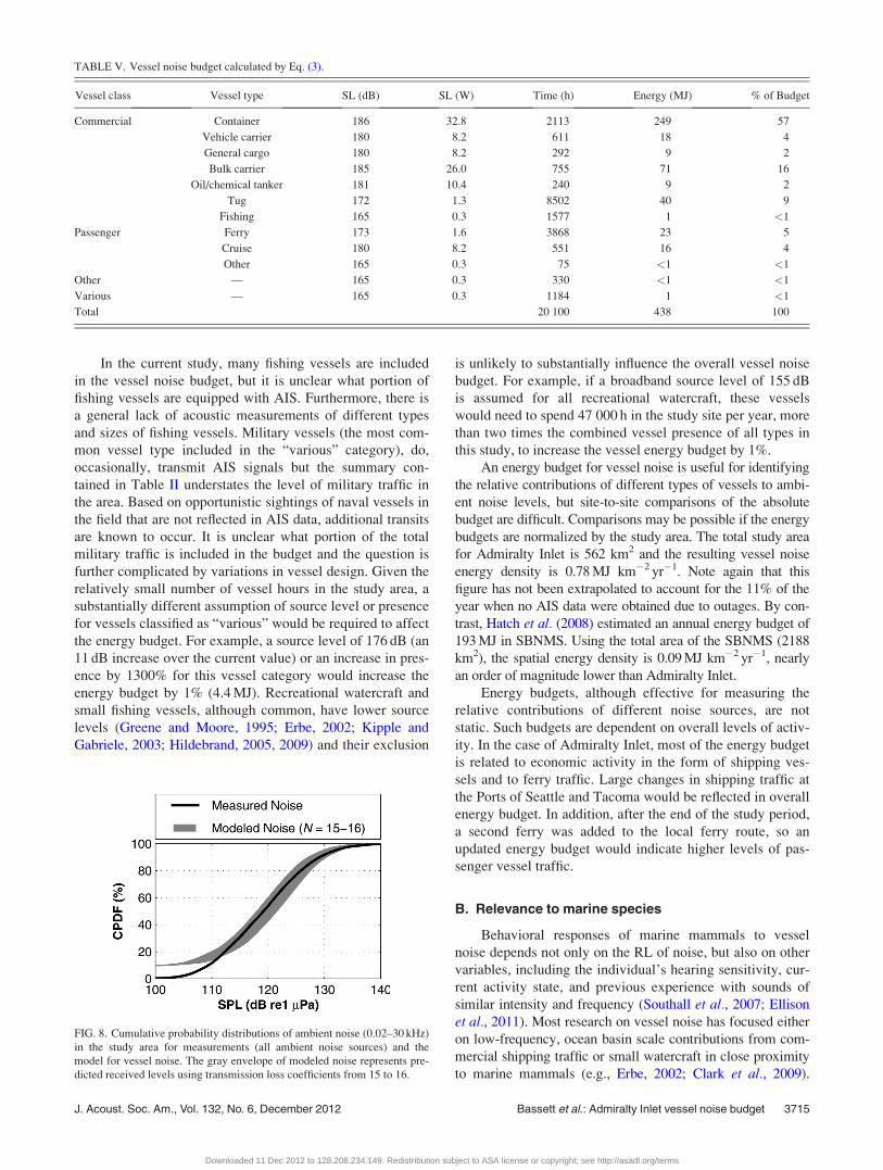
modeled and observed noise are presented in Fig. 8. Above

the 15th percentile, the measured noise distribution falls

within the model results for the N¼ 15–16 envelope [Eq.

(4)]. The good agreement between measured and modeled

results suggests that most of the ambient noise variability at

the site can be explained by AIS-equipped vessel traffic.

During quieter periods, other noise sources, such as distant

shipping, wind, and waves, are likely to dominate. Limited

land-based commercial and industrial activity in the immedi-

ate vicinity of the study area also suggests that noise from

other anthropogenic sources is insignificant. Based on tem-

poral variability explained by vessel traffic in Fig. 8, a cumu-

lative energy flux distribution (not shown) reveals that

vessels traffic accounts for 99% of the acoustic energy flux

at the measurement location.

V. DISCUSSION

A. Energy budget

The sensitivity of the energy budget depends primarily

on the source levels assigned to cargo ships, tugs, and pas-

senger vessels due to their temporal dominance. For each

1 dB increase in source levels attributed to tugs and ferries,

the total energy added to the budget increases by 10 MJ (2%)

and 3 MJ (<1%), respectively. Because these three vessel

types spend an order of magnitude more time in the study

area than others, the total budget is relatively insensitive to

source levels attributed to traffic of other vessel types (with

the exception of fishing vessels). Therefore, proper attribu-

tion of source levels for less common vessel types, while de-

sirable, is relatively unimportant.

AIS data are a useful tool for quantifying the densities of

commercial and passenger vessel traffic. However, small rec-

reational watercraft and fishing vessels, neither of which is

required to use AIS, are also common in the area. The vessel

noise budget does not include the contribution from vessels

without AIS transponders, and this is a notable limitation

if relying on AIS as the sole source of vessel traffic data.

TABLE IV. Estimated source levels (0.02–30 kHz) based on received levels (0.02–30 kHz) for selected ships.

Date/time Name Vessel type LOA (m) SOG (kn) CPA (km) RL (dB) SL (dB)

February 15, 2011 9:20 Victoria Clipper IV Ferry 36 30.8 1.65 121 170

February 16, 2011 9:18 Victoria Clipper Ferry 40 30.5 1.26 121 168

February 13, 2011 6:51 Eagle Tug 32 9.6 1.22 127 173

February 16, 2011 4:41 Valor Tug 30 8.4 1.46 121 168

February 16, 2011 12:25 Lela Joy Tug 24 4.9 1.15 126 172

February 15, 2011 4:14 Pacific Eagle Tug 28 8.2 1.36 118 165

February 20, 2011 18:28 Shannon Tug 28 9.3 0.58 129 171

February 11, 2011 23:30 James T Quigg Tug 30 7.9 1.42 120 167

February 19, 2011 6:23 Island Scout Tug 30 5.8 1.47 127 174

February 20, 2011 12:44 Chief Tug 34 11.4 1.23 128 174

February 12, 2011 1:57 Horizon Kodiak Container 217 20.1 1.53 132 179

February 12, 2011 3:02 Hong Yu Bulk carrier 226 13.6 1.52 135 182

February 12, 2011 3:44 Great Land Vehicle carrier 243 23 1.36 137 184

February 12, 2011 11:30 Ever Excel Container 300 18.2 2.78 132 183

February 14, 2011 7:42 Ever Excel Container 300 20.8 1.93 136 186

February 12, 2011 22:24 Hanjin Hamburg Container 335 23.8 2.82 133 185

February 14, 2011 2:39 Hanjin Hamburg Container 335 21.3 1.51 137 185

February 14, 2011 9:02 CSK Unity Bulk carrier 225 13.6 2.07 128 178

February 14, 2011 19:07 CMA CGM Carmen Container 334 23.8 1.46 136 183

February 14, 2011 19:56 MSC Kim Container 265 22.7 1.35 136 183

February 16, 2011 9:00 Bremen Bridge Container 279 21.2 1.02 136 181

February 17, 2011 7:53 Hyundai Republic Container 305 24.7 1.49 136 184

February 17, 2011 22:34 Coastal Sea General cargo 55 12.5 1.36 129 176

February 21, 2011 0:14 Green Point Vehicle carrier 180 19.1 1.41 133 180



In the current study, many fishing vessels are included

in the vessel noise budget, but it is unclear what portion of

fishing vessels are equipped with AIS. Furthermore, there is

a general lack of acoustic measurements of different types

and sizes of fishing vessels. Military vessels (the most com-

mon vessel type included in the “various” category), do,

occasionally, transmit AIS signals but the summary con-

tained in Table II understates the level of military traffic in

the area. Based on opportunistic sightings of naval vessels in

the field that are not reflected in AIS data, additional transits

are known to occur. It is unclear what portion of the total

military traffic is included in the budget and the question is

further complicated by variations in vessel design. Given the

relatively small number of vessel hours in the study area, a

substantially different assumption of source level or presence

for vessels classified as “various” would be required to affect

the energy budget. For example, a source level of 176 dB (an

11 dB increase over the current value) or an increase in pres-

ence by 1300% for this vessel category would increase the

energy budget by 1% (4.4 MJ). Recreational watercraft and

small fishing vessels, although common, have lower source

levels (Greene and Moore, 1995; Erbe, 2002; Kipple and

Gabriele, 2003; Hildebrand, 2005, 2009) and their exclusion

is unlikely to substantially influence the overall vessel noise

budget. For example, if a broadband source level of 155 dB

is assumed for all recreational watercraft, these vessels

would need to spend 47 000 h in the study site per year, more

than two times the combined vessel presence of all types in

this study, to increase the vessel energy budget by 1%.

An energy budget for vessel noise is useful for identifying

the relative contributions of different types of vessels to ambi-

ent noise levels, but site-to-site comparisons of the absolute

budget are difficult. Comparisons may be possible if the energy

budgets are normalized by the study area. The total study area

for Admiralty Inlet is 562 km2 and the resulting vessel noise

energy density is 0.78 MJ km�2 yr�1. Note again that this

figure has not been extrapolated to account for the 11% of the

year when no AIS data were obtained due to outages. By con-

trast, Hatch et al. (2008) estimated an annual energy budget of

193 MJ in SBNMS. Using the total area of the SBNMS (2188

km2), the spatial energy density is 0.09 MJ km�2 yr�1, nearly

an order of magnitude lower than Admiralty Inlet.

Energy budgets, although effective for measuring the

relative contributions of different noise sources, are not

static. Such budgets are dependent on overall levels of activ-

ity. In the case of Admiralty Inlet, most of the energy budget

is related to economic activity in the form of shipping ves-

sels and to ferry traffic. Large changes in shipping traffic at

the Ports of Seattle and Tacoma would be reflected in overall

energy budget. In addition, after the end of the study period,

a second ferry was added to the local ferry route, so an

updated energy budget would indicate higher levels of pas-

senger vessel traffic.

B. Relevance to marine species

Behavioral responses of marine mammals to vessel

noise depends not only on the RL of noise, but also on other

variables, including the individual’s hearing sensitivity, cur-

rent activity state, and previous experience with sounds of

similar intensity and frequency (Southall et al., 2007; Ellison

et al., 2011). Most research on vessel noise has focused either

on low-frequency, ocean basin scale contributions from com-

mercial shipping traffic or small watercraft in close proximity

to marine mammals (e.g., Erbe, 2002; Clark et al., 2009).

TABLE V. Vessel noise budget calculated by Eq. (3).

Vessel class Vessel type SL (dB) SL (W) Time (h) Energy (MJ) % of Budget

Commercial Container 186 32.8 2113 249 57

Vehicle carrier 180 8.2 611 18 4

General cargo 180 8.2 292 9 2

Bulk carrier 185 26.0 755 71 16

Oil/chemical tanker 181 10.4 240 9 2

Tug 172 1.3 8502 40 9

Fishing 165 0.3 1577 1 <1

Passenger Ferry 173 1.6 3868 23 5

Cruise 180 8.2 551 16 4

Other 165 0.3 75 <1 <1

Other — 165 0.3 330 <1 <1

Various — 165 0.3 1184 1 <1

Total 20 100 438 100

FIG. 8. Cumulative probability distributions of ambient noise (0.02–30 kHz)

in the study area for measurements (all ambient noise sources) and the

model for vessel noise. The gray envelope of modeled noise represents pre-

dicted received levels using transmission loss coefficients from 15 to 16.



Numerous studies of marine mammal reactions to vessels sug-

gest that exposure to elevated vessel noise may alter marine

mammal behavior and increase stress hormone levels with

potential biological consequences (Buckstaff, 2004; Foote

et al., 2004; Holt et al., 2009; Rolland et al., 2012).

Broadband SPLs at the study site regularly exceed

120 dB [Fig. 3(c)], the current acoustic criterion for behav-

ioral harassment of marine mammals for continuous sound

types (120 dB re 1 lPa) in the United States (NMFS, 2005).

The current acoustic criteria are based on broadband meas-

urements and do not take into account frequency-specific

hearing capabilities that differ among marine mammal

groups. The weighted cumulative probability distributions of

received levels for each marine mammal functional hearing

group are shown in Fig. 3 in an effort to address variation in

hearing capabilities among groups. Because low-frequency

cetaceans and pinnipeds have relatively flat hearing sensitiv-

ity over the frequencies associated with commercial ship-

ping, their received levels approach the broadband receiver

idealization. However, the M-weighting functions for mid-

and high-frequency cetaceans start to roll off at frequencies

less than 1 kHz, where the majority of acoustic energy asso-

ciated with commercial ships is concentrated. Consequently,

perceived mean received levels for mid- and high-frequency

cetaceans based on these weighting functions are, on aver-

age, at least 5 dB lower. As previously mentioned, noise

from recreational vessels is unlikely to contribute substan-

tially to the vessel noise budget in the study location. None-

theless, noise from these smaller vessels may be of concern

to mid- and high-frequency cetaceans because their energy is

concentrated at higher frequencies than commercial ships

(Erbe, 2002). This points to a general need for frameworks

that are able to treat anthropogenic noise in a more biologi-

cally relevant manner.

At close range (e.g., within 10 km of the source), different

types of vessel activity increase noise levels across a broader

range of frequencies than is often considered. Below 1 kHz,

ship traffic regularly increases noise levels by 25 dB above

background levels. At higher frequencies, extending up

to 30 kHz, one-third octave band SPLs regularly increase by

10–20 dB [Figs. 3(b) and 6]. These increases in ambient noise

from shipping traffic are sufficient to regularly mask commu-

nicative sounds used by many marine mammals unless they

are able to compensate vocally (Holt et al., 2009).

Because the Main Basin of Puget Sound is also rela-

tively narrow (approximately 10–20 km wide), large com-

mercial vessels transiting the area are expected to elevate

broadband ambient noise levels over the entire width of the

channel to levels in excess of 120 dB. The hydrophone

deployments in this study are well outside (>1 km) of the

shipping lanes and, as shown in Fig. 1(c), few vessels

passed directly over the deployed hydrophones. As a result,

moderately higher recorded broadband SPLs would be

expected mid-channel, where vessel densities are greater.

The proximity to ferry routes, shipping lanes, and popu-

lated coastal communities are common throughout Puget

Sound. Therefore, the noise levels observed in this study

area may be extended, with due caution, to other areas in

the region.

VI. CONCLUSION

One year of AIS data is paired with hydrophone record-

ings from a site in northern Admiralty Inlet, Puget Sound,

WA to assess ambient noise levels and the contribution of

vessel noise to these levels. Admiralty Inlet experiences a

high level of vessel traffic due to cargo ships bound for

major ports, tugs towing barges, and ferries transporting pas-

sengers and vehicles. Results suggest that ambient noise lev-

els between 20 Hz and 30 kHz are largely driven by vessel

activity and that the increases associated with vessel traffic

are biologically significant.

Throughout the year, at least one AIS-transmitting ves-

sel is within the study area 90% of the time and multiple ves-

sels are present 68% of the time. A vessel noise budget is

constructed to assess the relative contributions of different

vessel types to underwater noise levels at the site. Results

show cargo vessels account for 79% of the acoustic energy

in the vessel noise budget. Passenger ferries and tugs have

lower source levels but spend substantially more time in the

study site and contribute 18% of the energy in the budget.

Recreational watercraft contribute to ambient noise levels

but are unlikely to contribute substantially to the overall ves-

sel noise budget due to limited presence and lower source

levels. All vessels generate acoustic energy at frequencies

relevant to all marine mammal functional hearing groups.

A basic model for received levels accounts for vessel

types, distance to the hydrophone, and specified characteris-

tic source levels for each vessel type. The model explains

85% of the temporal variability in observations and demon-

strates the predominance of maritime traffic in the overall

noise budget at the site.

ACKNOWLEDGMENTS

Thanks to Joe Talbert and Alex deKlerk for their work

designing, assembling, deploying, and recovering the tripods.

Thanks to Captain Andy Reay-Ellers, the captain of the R/V

Jack Robertson. Ongoing studies at the site have been moti-

vated by the Snohomish Public Utility District and without

their interest in tidal energy this study would not have been

undertaken. Washington State Parks allowed for the place-

ment of the AIS system on Admiralty Head Light-house and

helped reboot the system after a number of power outages.

We thank the anonymous reviewers for their comments on

the content and structure of the manuscript. Funding pro-

vided by U.S. Department of Energy Award No. DE-

EE0002654. Student support provided to C.B. by National

Science Foundation Award No. DGE-0718124.

APPENDIX A: TRANSMISSION LOSSESCOEFFICIENT

A single-valued transmission loss model [i.e., 15 log(r)]

assumes that the transmission losses are independent of the

location of a vessel relative to the hydrophone receiver.

Given changing bathymetric profiles between the ship and

receiver as a vessel travels in the shipping lanes, the assump-

tion of angular and range independence must be verified. To

justify the use of a single-valued transmission loss model, a



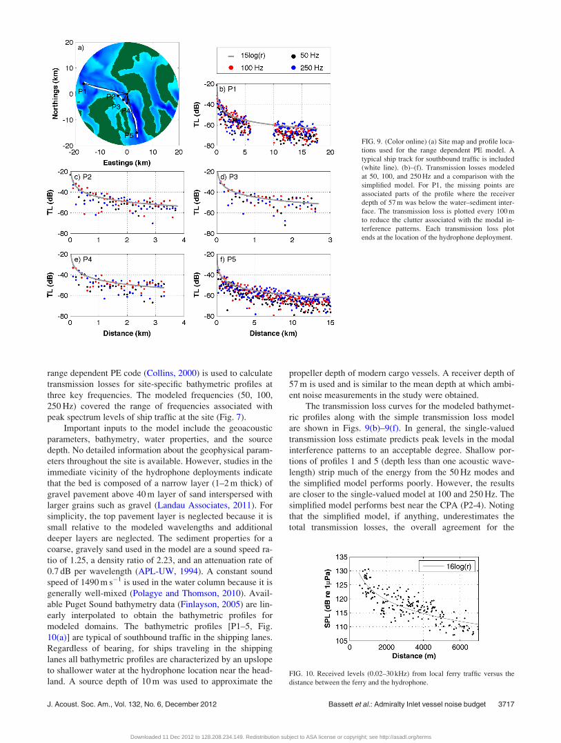
range dependent PE code (Collins, 2000) is used to calculate

transmission losses for site-specific bathymetric profiles at

three key frequencies. The modeled frequencies (50, 100,

250 Hz) covered the range of frequencies associated with

peak spectrum levels of ship traffic at the site (Fig. 7).

Important inputs to the model include the geoacoustic

parameters, bathymetry, water properties, and the source

depth. No detailed information about the geophysical param-

eters throughout the site is available. However, studies in the

immediate vicinity of the hydrophone deployments indicate

that the bed is composed of a narrow layer (1–2 m thick) of

gravel pavement above 40 m layer of sand interspersed with

larger grains such as gravel (Landau Associates, 2011). For

simplicity, the top pavement layer is neglected because it is

small relative to the modeled wavelengths and additional

deeper layers are neglected. The sediment properties for a

coarse, gravely sand used in the model are a sound speed ra-

tio of 1.25, a density ratio of 2.23, and an attenuation rate of

0.7 dB per wavelength (APL-UW, 1994). A constant sound

speed of 1490 m s�1 is used in the water column because it is

generally well-mixed (Polagye and Thomson, 2010). Avail-

able Puget Sound bathymetry data (Finlayson, 2005) are lin-

early interpolated to obtain the bathymetric profiles for

modeled domains. The bathymetric profiles [P1–5, Fig.

10(a)] are typical of southbound traffic in the shipping lanes.

Regardless of bearing, for ships traveling in the shipping

lanes all bathymetric profiles are characterized by an upslope

to shallower water at the hydrophone location near the head-

land. A source depth of 10 m was used to approximate the

propeller depth of modern cargo vessels. A receiver depth of

57 m is used and is similar to the mean depth at which ambi-

ent noise measurements in the study were obtained.

The transmission loss curves for the modeled bathymet-

ric profiles along with the simple transmission loss model

are shown in Figs. 9(b)–9(f). In general, the single-valued

transmission loss estimate predicts peak levels in the modal

interference patterns to an acceptable degree. Shallow por-

tions of profiles 1 and 5 (depth less than one acoustic wave-

length) strip much of the energy from the 50 Hz modes and

the simplified model performs poorly. However, the results

are closer to the single-valued model at 100 and 250 Hz. The

simplified model performs best near the CPA (P2-4). Noting

that the simplified model, if anything, underestimates the

total transmission losses, the overall agreement for the

FIG. 10. Received levels (0.02–30 kHz) from local ferry traffic versus the

distance between the ferry and the hydrophone.

FIG. 9. (Color online) (a) Site map and profile loca-

tions used for the range dependent PE model. A

typical ship track for southbound traffic is included

(white line). (b)–(f). Transmission losses modeled

at 50, 100, and 250 Hz and a comparison with the

simplified model. For P1, the missing points are

associated parts of the profile where the receiver

depth of 57 m was below the water–sediment inter-

face. The transmission loss is plotted every 100 m

to reduce the clutter associated with the modal in-

terference patterns. Each transmission loss plot

ends at the location of the hydrophone deployment.



typical variations in profiles justifies the use of the single-

valued transmission loss model to reconstruct noise levels

and estimate SL.

APPENDIX B: FERRY SL

To estimate the source level of the most commonly

present vessel, the local ferry, and empirically estimate the

transmission loss coefficient, acoustic data throughout the

year were used. Current velocity and AIS data were used to

screen for periods in which the currents were weak

(<0.4 m s�1) and the local ferry “Chetzemoka” was the only

vessel in the study area. Further manual screening was done

to remove recordings of the ferry that were not consistent

with other ferry measurements and were deemed to be likely

contaminated by other noise sources (e.g., a non-AIS

equipped vessel). The source level and transmission loss

coefficient were calculated by regressing the broadband RL

against the log of the distance, in meters, and performing a

least squares linear regression analysis. In this instance, esti-

mation of the transmission loss coefficient for the ferry was

limited by the Port Townsend ferry terminal at a distance of

7 km. The resulting regression fit yielded a source level of

173 dB re 1 lPa at 1 m (y intercept) and a transmission loss

coefficient of 16 dB (slope). Figure 10 shows the results of

the regression with the RL plotted against the distance to the

ferry on a linear scale.

1For smaller vessels, including small U.S. flagged cargo vessels, tugs, fish-

ing vessels, and vessels falling into the categories of “other” and

“various,” registration data (http://www.boatinfoworld.com/) were used.

Searches by vessel name result in information that includes vessel

type, size, and length, which were cross-checked against AIS data. Simi-

larly, online fleet information was used for many commercial vessels to

cross-check registration and AIS data (e.g., http://westerntowboat.com/

Tugs/ to confirm registration data for the vessel Western Mariner; http://

www.cosco.com/en/fleet/ to confirm COSCO fleet information).

Ainslie, M., and McColm, J. (1998). “A simplified formula for viscous and

chemical absorption in sea water,” J. Acoust. Soc. Am. 103, 1671–1672.

Applied Physics Laboratory (1994). “High-frequency ocean environmental

acoustic models handbook,” Technical Report TR 9407, Applied Physics

Laboratory at the University of Washington.

Arveson, P. T., and Vendittis, D. J. (2000). “Radiated noise characteristics

of a modern cargo ship,” J. Acoust. Soc. Am. 107, 118–129.

Buckstaff, K. (2004). “Effects of watercraft noise on the acoustic behavior

of bottlenoise dolphins, Tursiops truncatus, in Sarasota, Florida,” Marine

Mammal Sci. 20, 709–725.

Clark, C., Ellison, W., Southall, B., Hatch, L., Van Parijs, S., Frankel, A.,

and Ponirakis, D. (2009). “Acoustic masking in marine ecosystems: Intu-

itions, analysis, and implications,” Mar. Ecol.: Prog. Ser. 395, 201–222.

Collins, M. D. (2000). “User’s guide for RAM versions 1.0 and 1.0p,” Naval

Research Laboratory, Washington, DC.

Dahl, P., Miller, J., Cato, D., and Andrew, R. (2007). “Underwater ambient

noise,” Acoust. Today 3, 23–33.

Ellison, W., Southall, B., Clark, C., and Frankel, A. (2011). “A new context-

based approach to assessing mammal behavioral responses to anthropo-

genic sounds,” Conserv. Biol. 26, 1–8.

Erbe, C. (2002). “Underwater noise of whale-watching boats and potential

effects on killer whales (Orcinus orca), based on acoustic impact model,”

Marine Mammal Sci. 18, 394–418.

Federal Register (2003). “Automatic identification system; vessel carriage

requirements,” Coast Guard, U.S. Department of Homeland Security, pp.

60559–60570.

Finlayson D. P. (2005). “Combined bathymetry and topography of the Puget

Lowland, Washington State,” http://www.ocean.washington.edu/data/

pugetsound/ (Last viewed July 16, 2012).

Foote, A., Osborne, R., and Hoelzel, A. (2004). “Whale-call response to

masking boat noise,” Nature (London) 428, 910.

Frisk, G. V. (2012). “Noiseonomics: The relationship between ambient noise

levels in the sea and global economic trends,” Sci. Rep. 107, 1–4.

Gray, L., and Greeley, D. (1980). “Source level model for propeller blade rate

radiation for the world’s merchant fleet,” J. Acoust. Soc. Am. 67, 516–522.

Greene, C. R., Jr., and Moore, S. (1995). “Man-made noise,” in MarineMammals and Noise, edited by J. W. Richardson, C. R. Greene, Jr., C. I.

Malme, and D. H. Thompson (Academic, San Diego), pp. 101–158.

Harati-Mokhtari, A., Wall, A., Brooks, P., and Wang, J. (2007). “Automatic

identification system (AIS): Data reliability and human error

implications,” J. Navig. 60, 373–389.

Hatch, L., Clark, C., Merrick, R., Van Parijs, S., Ponirakis, D., Schwehr, K.,

Thompson, M., and Wiley, D. (2008). “Characterizing the relative contri-

butions of large vessels to total ocean noise fields: A case study using the

Gerry E. Studds Stellwagen Bank National Marine Sanctuary,” Environ.

Manage. (N.Y.) 42, 735–752.

Hildebrand, J. (2004). “Sources of anthropogenic sound in the marine envi-

ronment,” Technical Report, Report to the Policy on Sound and Marine

Mammals: An International Workshop, U.S. Marine Mammals Commis-

sion and Joint Conservation Committee U.K., London.

Hildebrand, J. (2005). “Impacts of anthropogenic sound,” in Marine Mam-mal Research: Conservation Beyond Crisis, edited by J. E. Reynolds, W.

F. Perin, R. R. Reeves, S. Montgomery, and T. J. Ragen (The Johns Hop-

kins University Press, Baltimore, MD), pp. 101–124.

Hildebrand, J. (2009). “Anthropogenic and natural sources of ambient noise

in the ocean,” Mar. Ecol.: Prog. Ser. 395, 5–20.

Holt, M., Noren, D., Veirs, V., Emmons, C., and Veirs, S. (2009). “Speaking

up: Killer whales (Orcinus orca) increase their call amplitude in response

to vessel noise,” J. Acoust. Soc. Am. 125, EL27–EL32.

Kipple, B. (2004a). “Coral Princess underwater acoustic levels,” Technical

Report (Naval SurfaceWarfare Center, Bremerton Detachment).

Kipple, B. (2004b). “Volendam underwater acoustic levels,” Technical

Report (Naval Surface Warfare Center, Bremerton Detachment).

Kipple, B., and Gabriele, C. (2003). “Glacier Bay watercraft noise: Report to

Glacier Bay National Park by the Naval Surface Warfare Cent-Detachment

Bremerton,” Technical Report No. NSWCCD-71-TR-2003/522.

Landau Associates (2011). “Preliminary geologic characterization: Proposed

tidal turbine site Island County, Washington,” Technical Report for Sound

and Sea Technology and Snohomish County, P. U. D., September 6, 2011.

Lee, S., Kim, S., Lee, Y., Yoon, J., and Lee, P. (2011). “Experiment on

effect of screening hydrophone for reduction of flow-induced ambient

noise in ocean,” Jpn. J. Appl. Phys. 50, 1–2.

McDonald, M. A., Hildebrand, J. A., and Wiggins, S. M. (2006). “Increases

in deep ocean ambient noise in the Northeast Pacific west of San Nicolas

Island, California,” J. Acoust. Soc. Am. 120, 711–718.

McDonald, M. A., Hildebrand, J. A., Wiggins, S. M., and Ross, D. (2008).

“A 50 year comparison of ambient ocean noise near San Clemente Island:

A bathymetrically complex coastal region off Southern California,” J.

Acoust. Soc. Am. 124, 1985–1992.

McKenna, M., Ross, D., Wiggins, S., and Hildebrand, J. (2012).

“Underwater radiated noise from modern commercial ships,” J. Acoust.

Soc. Am. 131, 92–103.

National Marine Fisheries Service (NMFS) (2005). “Endangered fish

and wildlife; notice of intent to prepare an environmental impact

statement,” Federal Register 70(7), 1871–1875 (Docket No. 05-525, 11

January 2005).

National Marine Fisheries Service (NMFS) (2006). “Endangered and threat-

ened species; designation of critical habitat for Southern Resident killer

whales,” Federal Register 71(229), 69054–69070 (Docket No.

060228057-6283-02, 29 November 2006).

National Research Council of the U.S. National Academies (NRC) (2000).

Marine Mammals and Low-Frequency Sound (National Academy Press,

Washington, DC), pp. 7, 76.


Ocean Noise and Marine Mammals (National Academy Press, Washing-

ton, DC), pp. 6, 65–67, 89, 93, 128.


Marine Mammal Populations and Ocean Noise: Determining When OceanNoise Causes Biologically Significant Effects (National Academy Press,

Washington, DC), p. 14.



Orlanski, I. (1975). “A rational subdivision of scales for atmospheric proc-

esses,” Bull. Am. Meteorol. Soc. 56, 527–530.

Polagye, B., and Thomson, J. (2010). “Admiralty Inlet water quality

survey report: April 2009–February 2010,” Technical Report, Northwest

National Marine Renewable Energy Center, University of Washington,

Seattle, WA.

Rolland, R. M., Parks, S. E., Hunt, K. E., Castellote, M., Corkeron, P. J.,

Nowacek, D. P., Wasser, S. K., and Kraus, S. D. (2012). “Evidence that

ship noise increases stress in right whales,” Proc. R. Soc. London, Ser. B

279, 2363–2368.

Ross, D. (1976). Mechanics of Underwater Noise (Permagon, Elmsford,

NY), pp. 272, 279–280.

Schwehr, K. (2010). “Python software for processing AIS data. v0.43,”

http://vislab-ccom.unh.edu/schwehr/software/noaadata (Last viewed

January 29, 2011).

Scrimger, P., and Heitmeyer, R. (1991). “Acoustic source-level measure-

ments for a variety of merchant ships,” J. Acoust. Soc. Am. 89, 691–699.

Southall, B. (2005). “Shipping noise and marine mammals: A forum for sci-

ence, management, and technology,” Technical Report, Final Report of

the National Oceanic and Atmospheric Administration (NOAA) Interna-

tional Symposium, U.S. NOAA Fisheries, Arlington, VA, May 18–19,

2004.

Southall, B., Bowles, A., Ellison, W., Finneran, J., Gentry, R., Greene, C.,

Jr., Kastak, D., Ketten, D., Miller, J., Nachtigall, P., Richardson, W.,

Thomas, J., and Tyack, P. (2007). “Marine mammal noise exposure crite-

ria: Initial scientific recommendations,” Aquat. Mamm. 33, 411–521.

Thomson, J., Polagye, B., Durgesh, B., and Richmond, M. C. (2012).

“Measurements of turbulence at two tidal energy sites in Puget Sound,

WA,” IEEE J. Ocean. Eng. 37, 363–374.

Thorne, P. (1990). “Seabed generation of ambient noise,” J. Acoust. Soc.

Am. 87, 149–153.

Thorne, P. D., Heathershaw, A. D., and Troiano, L. (1984). “Acoustic detec-

tion of seabed gravel movement in turbulent tidal currents,” Mar. Geol.

54, M43–M48.

Trevorrow, M. V., Vasiliev, B., and Vagle, S. (2008). “Directionality and

maneuvering effects on a surface ship underwater acoustic signature,”

J. Acoust. Soc. Am. 107, 767–778.

Urick, R. (1967). Principles of Underwater Sound for Engineers (McGraw-

Hill, New York), pp. 164–165.

Van Parijs, S., Clark, C., Sousa-Lima, R., Parks, S., Rankin, S., Risch, D.,

and Van Opzeeland, I. (2009). “Management and research applications of

real-time and archival passive acoustics sensors over varying temporal and

spatial scales,” Mar. Ecol.: Prog. Ser. 395, 21–36.

Veirs, S., and Veirs, V. (2005). “Average levels and power spectra of ambi-

ent sound in the habitat of southern resident orcas,” NMFS Contract

Report No. AB133F05SE6681.

Wenz, G. (1962). “Acoustic ambient noise in the ocean: Spectra and

sources,” J. Acoust. Soc. Am. 34, 1936–1956.



avessel noise budget for admiralty inlet, puget sound...

Documents