AWS/TN-87/002REVISED

AID-A Yg~ p/,

ISENTROPIC ANALYSIS AND INTERPRETATION:

OPERATIONAL APPLICATIONS TO SYNOPTIC

AND MESOSCALE FORECAST PROBLEMS

• DTICELECTE

MAY 2 2 1989 By

" Dr. James T. MooreD. -° ,iSaint Louis Universityeparte~t of Earth and Atmospheric Sciences

1'.0 Box 8099-Laclede StationSt. Louis, Missouri 63156

AUGUST 1987

REVISED MAY 1989

APPRovED FOR PUBLIC RELEASE; DISTRIBUTION IS UNLIMITED.

AIR WEATHER SERVICE (MAC)Scott Air Force Base, Illinois, 62225-5008

89 to

REVIEM AAV APPROVAL STATE ME

AWS/TN-87/OO2, Isentropic Analysis and Interpretation: Operational Applications to Synoptic andMesoscale Forecast Problems, August 1987, is approved for public release. There is no objection tounlimited distribution of this document to the public at large, or by the Defense TechnicalIntorndtion Center (DTIC) to the National Technical Information Service (NTIS).

This document has been reviewed and is approved for publication.

/,~

GEORGE ANIGUICHI, G-13Forecag'ting Services DivisionDirectorate of Aerospace Services,DCS/Aerospace SciencesReviewing Official

FOR THE COMMANDER

DOUGLAS 'A. ABBOTT, Clonel, USAFAsst DCS/Aerospace Sciences

S

S

I

'UNCLASSIFIEDREPORT DCUMENTATION PAGE

la. Report Security Classification: UNCLASSIFIED

3. Oistribution/Availability of Report: Approved for public release; distribution is unlimited.

4. Performino Oroanization ReDort Number: AWS/TN-87/002

6a. Name of Performing_Organization: HQ AWS

6b. Office Symbol: DNTS

6c. Address: Scott AFB, IL 62208-5008

11. Title: Isentropic Analysis and Interpretation: Operational Applications to Synoptic andesoscaTorecast Problems

12. Personal Author: Dr James T. Moore, Saint Louis University, Department of Earth and AtmosphericSciences, P.O. Box 8099-LaClede Station, St Louis, MO 63156

13a. Type of Report: Technical note

14. Date of Report: August 1987

15. .ae Count: 93

17. COSATI Codes: Field--04, Group--02

18. Subject Terms: METEOROLOGY, WEATHER FORECASTING, AVIATION FORECASTING, WEATHER ANALYSIS,ISENTROP1C ANALYSIS, ISENTROPIC COORDINATE SYSTEM, CONSTANT PRESSURE ANALYSIS, TRAJECTORY ANALYSIS,TROPOPAUSE FOLDING PROCESS, psi charts, sigma charts, thermal wind, static stability, vorticity,condensation pressure, condensation ratio, condensation difference, streamlines, trajectories,freezing 1e e icing, clear air turbulence, overrunning convection.

19. Abstract. A basic review of the isentropic coordinate system, including its advantages anddisadvantages for operational use. The primitive equations in isentropic coordinate form arediscussed with emphasis on their physical meaning and interpretation. Isentropic analysis techniquesfor 'horizontalV-end cross sectional perspectives are described as aids for diagnostic analysis ofsynoptic scale weather systems. Numerous diagnostic variables are discussed; all can be excellenttools in identifying synoptic scale features helpful in forecasting cyclogenesis and regionssusceptible to strong convection. The final section presents specialized applications of isentropictechniques to weather analysis and forecasting, including: trajectory analysis, tropopause foldingprocess, short-term forecasting of severe weather threat areas, and aviation forecasting.

20. Distribution/Availability of Abstract: Same as report

21. Abstract Security Classification: UNCLASSIFIED Accesion For ]

22a. Name of Responsible Individual: George Taniguchi NTIS CFH. d'

DTIC TA' El22b. Telephone: 618 256-4741 (A576-4741) Unaicr, ',:i 0

22c. Office Symbol: AWS/DNTS Jutic

By" DtstrmLuti.onp

Avai';b!,tq Co'des

D Avil L1i or

PD1st

D FORM 14173 UNCLASSIFIErii

PREFACE

lefore the changeover to pressure coordinates in the early 1940's, isentropicanalysis was utilized extensively for diagnosing and forecasting weather systems.Since that time the advantages of the isentropic coordinate system and isentropicanalysis techniques have been neglected in the curricula of both universities andtraining centers. The 1960's and 1970's saw a resurgence of isentropic analysis inthe research community as it was well-suited to the needs of those studyingatmospheric flow on both the synoptic and mesoscales of motion. This mono-;:aph has been wriLen with the goai of presenting the isentropic viewpoint andmethods of diagnosis in one volume that can be easily accessible to the practicingoperational meteorologist. It is the author's hope that this information will helpincrease the use of isentropic analysis techniques in the field as a supplement tostandard constant pressure analyses as forecasters attempt to diagnose and predictthe three dimensional flow associated with precipitation systems.

I would like to acknowledge that motivation for this paper came from Dr.Lawrence Wilson of the Atmospheric Environment Service in Canada who wrote asimilar shorter papec for Canadian meteorologists. Several examples discussed inthis text are borrowed from his training paper. Also, Anderson (1984) wrote apaper for the National Weather Service (NWS) Western Region describing isentro-pic analysis which is frequently referenced.

The author would like to thank St. Louis University for offering a sabbaticleave during which time he was able to work on this manuscript. The people atthe NSSFC were also very supportive and offered ideas on strengthening the text.Dr. Joe Schaefer of SSD in CRI gave helpful suggestions which were appreciated.Friends at the NWSTC including Daryl Covey, Pete Chaston, and Dan Berkowitzwho will be implementing this material into the NWS training program are allappreciated for their support and enthusiasm for this project. Also, Dr. DaleNleyer, Nb'. George Taniguchi, Mr. George Horn and Mr. Michael Squires of theAir WXeather Service are to be thanked for their proofreading of the text. Last,but not least, the expert typing of Ms. Juanita Ryles and the assistance of Mr.Richard Nlolinaro are deeply appreciated.

NOTE: THE MAY 1989 REVISION REQUIRED REPLACEMENTOF THE FOLLOWING PAGES: 9, 10, 45,46,49,83,84, 85.

iii

CONTENT'S

I. INTRODUCTION ... . . . . . . . . . . . . . . . . . . . . . . . . . . . . . . . . . . . . . . . . .1.2. ISENTROPIC COORDINATE SYSTEM............................................................... 2A. Definition.......................................................................... 2B. History of Isentropic Analysis ....................................................... 4C. Advantages of Isentropic Analysis..................................................... 6D. Disadvantages of Isentropic Analysis................................................. 13E. Primitive Equations in Isentropic Coordinates......................................... 18F. Constructing an Isentropic Data Set from Rawinsonde Data .............................. 26

3. ISENTROPIC ANALYSIS TECHNIQUES............................................................ 28A. Psi Charts......................................................................... 28B. Sigma Charts ....................................................................... 31C. Cross Section Analysis Techniques.................................................... 37

1. Thermal Wind Relationship in Isentropic Coordinates.............................. 372. Isentropic Topography in the Vicinity of Upper Level Fronts and Jet Streaks ........ 38

D. Useful Diagnostic Variables Computed From Isentropic Data.............................. 441. Static Stability.............................................................. 442. Moisture Advection/Convergence................................................. 443. Adiabatic Vertical Motion...................................................... 444. Static Stability Tendency ..................................................... 455. Absolute Vorticity............................................................ 456. Potential Vorticity ........................................................... 457. Condensation Pressure ......................................................... 468. Condensation Ratio............................................................ 469. Condensation Difference ....................................................... 46

10 Streamlines .................................................................. 49

4. SPECIALIZED APPLICATIONS OF ISENTROPIC ANALYSES TO DIAGNOSTIC/FORECAST PROBLEMS............... 52A. Isentropic Trajectories............................................................. 52

1. Implicit Approach............................................................. 522. Explicit Approach............................................................. 563. Trajectory-derived Variables................................................... 57

B. Potential Vorticity and Tropopause Folding ........................................... 60C. Short Term Forecasting of Severe Convection Using Isentropic Analyses .................. 69D. Additional Applications............................................................. 70

1. Freezing Level and Icing ...................................................... 742. Clear Air Turbulence .......................................................... 743. Overrunning Convection ........................................................ 78

5. CONCLUDING COMMENTS ...................................................................... 80

6. REFERENCES .............................................................................. 81

iv

FISRES

Figure la. Salem, IL (SLO) Sounding for 1200 GMT 8 September 1986 .................................. 7Figure lb. Albuquerque, NM (ABQ) Sounding for 0000 GMT 5 September 1986 ............................ 7Figure Z. Typicdl vertical cross section diagrams ................................................ 11Figure 3. Cross section showing how isentropic surfaces appear in the vicinity of regions with

superadiabatic (SA) and neutral (N) lapse rates ...................................... 14Figure 4. Cross section showing how the vertical resolution of an area may vary

within a very stable (VS) and less stable (LS) region ................................ 16Figure 5. Soundings for progressively later time periods into the night (tI, t2, t3)

illustrating how radiational influences may change the pressure level atwhich a given isentropic surface is found ............................................ 16

Figure 6. Schematic diag-am depicting the stability changes that can take place inthe presence of diabatic heating/cooling ............................................. 22

Figure 7. Geostrophic wind scale for an isentropic surface on a polar stereographicprojection with a 1:15 million map scale ............................................. 24

Figure 8. Geostrophic wind scale for an isentropic surface on a polar stereographicprojection with a 1:10 million map scale ............................................. 25

Figure 9. Station model plot for psi charts ...................................................... 29Figure 10. Isobaric topography in the vicinity of fronts (a) and isobaric topography

associated with frontogenesis in the warm sector (b) ................................. 30Figure Ila. Isentropic pressure pattern in the vicinity of a strong, mature cold front ............. 30Figure 11b. Isentropic pressure pattern in the vicinity of a frontolysing cold front .............. 32Figure l1c. Isentropic pressure pattern in the vicinity of an occluding frontal system ............. 32Figure 12. Fronts indicated at the surface and schematic flow pattern around an occluded

cyclone as shown by the moisture lines in an isentropic surface in mid-air ........... 33Figure 13. Illustrating probable upslope motion of a moist current as deduced from the

relation of the moisture lines to the isobars on an isentropic surface ............... 33Figure 14. Flow pattern at different isentropic surfaces wOich leads to increasing

convective instability ............................................................... 33Figure 15. Station model plot for sigma charts .................................................... 35Figure 16. Wilson (1985) station model plot ....................................................... 36Figure 17. Plotting model used by ISENT (NWS Southern Region isentropic plotting program

used on AFOS), Little (1985) ......................................................... 36Figure 18. Schematic showing how stations are depicted with respect to the regression line

and their original positions ......................................................... 39Figure 19. Cross section illustrating the relationship between sloping isentropic surfaces

and the vertical wind shear .......................................................... 40Figure 20. Cross section plotting model ........................................................... 41Figure 21. Idealized and averaged picture for the annual mean or the spring and autumn seasons .... 42Figure 22. Condensation pressure (mb) vs. specific humidity for 283, 293, 303, and 313 K

isentropic surfaces .................................................................. 47Figure 23a. Isentropic condensation pressure pattern over a mature, strong cold front .............. 48Figure 23b. Isentropic condensation pressure pattern over an occluding frontal system .............. 48Figure 24. Condensation-pressure spread to cloud-conversion table ................................. 50Figure 25a. Isentropic streamlines in the vicinity of a strengthening cold front ................... 51Figure 25b. Isentropic streamlines in the vicinity of a weakening cold front ....................... 51Figure 26a. Isentropic surface, e = 45 0C, 0300 GMT 8 January 1953 ................................. 54Figure 26b. Isentropic surface, 0 = 45 °C, 1500 GMT 8 January 1953 ................................. 55Figure 27a. 330 K isentropic surface for 1200 GMT 10 May and 0000 GMT 11 May 1973 .................. 58Figure 27b. Trajectories computed for 1200 GMT 10 May through 0000 GMT 11 May 1973 on 330 K

isentropic surface using discrete model technique .................................... 59Figure 28a. 312 K 3-hour isentropic trajectories beginning 1700 GMT 10 April 1979 .................. 61Figure 28b. 312 K 3-hour delta M field for 1700-2000 GMT 10 April 1979 ............................. 61Figure 28c. 312 K 3-hour vertical motion field for 1700-2000 GMT 10 April 1979 ..................... 62Figure 29a. 500 mb surface for 0300 GMT 13 December 1953 ........................................... 64Figure 29b. Cross section along line A-B in Figure 29a ............................................. 64Figure 29c. 500 mb surface for 0300 GMT 14 December 1953 ........................................... 65Figure 29d. Cross section along line C-D in Figure 29c ............................................. 65Figure 29e. 500 mb surface for 0300 GMT 15 December 1953 ........................................... 66Figure 29f. Cross section along line E-F in Figure 29e ............................................. 66Figure 30a-b Vertical cross section from International Falls, MN (INL) to Denver, CO (DEN)

for 1200 GMT 18 February 1979 ........................................................ 67Figure 30c-d Vertical cross sections from Green Bay, WI (GRB) to Apalachicola, FL (AQQ)

for 0000 GMT 19 February 1979 ........................................................ 68Figure 31a. National Weather Service radar summary for 2035 GMT 10 April 1979 ...................... 71Figure 31b. Isentropic cross section for 1700 GMT 10 April 1979 .................................... 71Figure 31c. The Montgomery streamfunction for 306 K surface at 1700 GMT 10 April 1979 .............. 71Figure 31d. Adiabatic vertical motion and specific humidity for 306 K surface at 1700 GMT

10 April 1979 ........................................................................ 72

V

Figure 31e. Horizontal moisture convergence and low level stability for 306 K surfaceat 1700 GMT 10 April 1979 ............................................................ 72

Figure 31f. Low level stability flux for 304-308 K layer at 1700 GMT 10 April 1979 ................. 73Figure 31g. Composite chart for 1700 GMT 10 April 1979 ............................................. 73Figure 32. Schematic illustration of regions of clear air turbulence in the vicinity of

an upper level jet core and frontal zone ............................................. 7bFigure 33. Cross sections of potential temperature and wind speed and direction

at 0000 GMT 20 April 1971 ............................................................ 77Figure 34. Cross section of eqivalent potential temperature and wind components parallel to

the plane of the cross section .................. .................................... 79

vi

1. INTRODUCTIONThe motivation behind this paper is simple--I wanted to lay down the basic

concepts of isentropic analysis and interpretation for those people in the "frontlines" of meteorology, the practicing forecasters. Since the demise of the isentropiccoordinate system in the 1040's, few academic institutions or training centers havetaught isentropic meteorology as part of their synoptic or weather analysis andforecasting laboratory courses. More recently, that situation has been changing.However, there are several generations oif meteorologists who have never beenshown the advantages of isentropic analyses in diagnosing the current weather.Therefore, they are naturally reluctant to incorporate these charts into their dailyforecasting scheme. The success of systems such as AFOS (Automation of FieldOperations and Services) and McIDAS (Man-Computer Interactive DisplayAcquisition System) show that new and varied computer products can be incor-porated into the operational environment. However, if these products are to beefficiently and intelligently utilized, the end users (i.e., the forecasters) must beknowledgeable about the advantages and disadvantages of each new tool. AsDoswell (1986) notes, we need to consider training at least as much as technology.The technology makes it very easy for us to create isentropic data sets and ana-lyses. The training makes this not-so-new method of diagnosing atmospheric floweasy to use, understandable and useful.

Toward that end I will try to illustrate the advantages and disadvantages ofisentropic analysis in the diagnosis of weather patterns as a supplement to stan-dard constant pressure analyses. I will draw heavily on the work of otherresearchers (e.g., Danielsen, Reiter, Uccellini, Petersen, Namias, Rossby, Wilson,Anderson) who have proven isentropic analyses effectiveness in diagnostic workthrough numerous case studies. References will be given so that the adventure-some reader can delve into some of the topics we discuss in greater detail. Forthat reason this paper does not attempt to be an exhaustive guide for isentropicmeteorology. Mathematics will be used but minimized for fear of boring or disen-franehising the reader. Emphasis instead will be placed upon conceptualization ofideas rather than heady dynamics. This is especially important in isentropicanalysis since isentropic surfaces are truly three-dimensional, unlike the quasitwo-dimensional pressure surfaces. Our experience at St. Louis University in thesynoptic laboratory is that it takes several weeks for students to get over theirtwo-dimensional, constant pressure biases to visualize three-dimensional isentropicflow. It is much like the transition for A. Square, the key character in Flatland byEdwin A. Abbott (1052), in going from Flatland to the three-dimensional world ofSphereland (Burger, 1065). This author encourages the reader to read both Flat-land and Sphereland as they are useful exercises in visualization; references aregiven at the end of this paper.

Finally, I want to acknowledge that motivation for this paper came from Dr.Laurence Wilson of the Atmospheric Environment Service in Canada who wrote asimilar shorter paper for Canadian meteorologists. Several examples discussed inthis text are borrowed from his training paper. Also Anderson (1984) wrote apaper describing isentropic analysis for the National Weather Service's (NWS)Western Region which is frequently referenced.

m mm m mmm m mmmmm1

2. ISENTROPIC COORDINATE SYSTEM

A. Definition

One must first begin with the concept of an adiajatic process as applied to afictitious parcel of air with a volume of roughly 1 m . During an adiabatic pro-cess an air parcel will experience no heat exchange with its environment; i.e., noheat is added or taken away from the parcel. In terms of the first law of thermo-dynamics we write,

dh = 0 = CdT - adP (1)

Since a = RT/P we can write (1) as:

dT R dPT cV- (2)T Cp P

Following Hess (1959), if we integrate from some temperature, T, and pressure, P,to a temperature, 0, at 1000 mb, we obtain:

_1000.o = T( - -) (3)

where t =- R/C p"The temperature, 0, is physically defined as the temperature that a parcel of

air would have if it were compressed (or expanded) adiabatically from its originalpressure to 1000 mb. It is known as potential temperature and is a conservativeproperty for parcels of air with no changes in heat due to such processes assolar/terrestrial radiation, mixing with environmental air that has a different tem-perature, and latent heating/evaporative cooling. Although these restrictionswould seem to make the application of this thermodynamic variable limited thereis empirical evidence that such "diabatic" heating and cooling processes are usuallysecondary in importance for temporal scales on the order of the synoptic. Somepeople (such as the author) would also argue that one could extend this approxi-miation to meso a scales of motion under certain conditions.

Hess (1959) also shows that the entropy of an air parcel, 0, is related to itspotential temperature as:

O= CplnO + const (4)

So a parcel which moves dry adiabatically not only conserves its potential tem-perature but also its entropy. A surface composed of parcels whose potential tel.-peratures are equal is described as an equal entropy or isentropic surface. In

2

thermodynamics we are told that entropy is a measure of the disorder of a sys-tem. However, operational meteorologists have little use for this concept. Thus,aside from using the term isentropic, we meteorologists prefer to use potentialtemperature as a variable rather than entropy, which carries more of a mysticalaspect!

In the troposphere the atmosphcre is, on the average, stable; i.e., -T/acZ --y < 9.5*C/kin, typically -yenv r 6.5 *C/km. In such an atmosphere thepoten'ial temperature can be shown by (5) to increase with height.

I ae (Fd-1') (5)a az T

In (5) F is the dry adiabatic lapse rate and -y is the actual or environmental lapserate. Under stable conditions ' < rd, so aOlaZ > 0 meaning 0 increases withheight. If the lapse rate is neutral then -y = rd and aO/aZ = 0; i.e., 0 is constantwith height. If -y > F the lapse rate is superadiabatic and 0 decreases withheight. Futhermore, as Aossby, et al., (1937) note, the potential temperature alsoincreases southward at about the same rate as the dry bulb temperature. So thetroposphere may be envisioned as being composed of a great number of isentropiclayers which gradually descend from cold polar regions to warmer subtropical lati-tudes. As one ascends from the troposphere into the stratosphere, where theatmosphere is very stable, isentropic surfaces become compacted in the vertical.This attribute makes them extremely valuable for resolving upper-level stablefrontal zones in the presence of upper tropospheric wind maxima or jet streaks.Thus, in a stably stratified atmosphere; i.e., -aT/8Z < 9.8 * C/km, potential tem-perature can be an excellent vertical coordinate--especially since it increases withheight, thereby avoiding the headaches of dealing with a vertical coordinate(namely pressure) which decreases with height.

Rossby, et al., (1937) and later Blackadar and Dutton (1970) note that it isnecessary to "tag" a parcel with more than its potential temperature since on anisentropic surface all parcels "look alike". A second natural "tag" would be mixingratio or specific humidity, both quantities which are also conserved during dryadiabatic ascent/descent. Another possible "tag" (which will be discussed later) ispotential vorticity. It should be no surprise, then, that the three-dimensional tran-sport of moisture on a vertically sloping isentropic surface should display goodspatial and temporal continuity. As will be shown later, this has important diag-nostic and prognostic implications for the movement of both moist and drytongues in low-middle levels of the troposphere.

Meanwhile, one might ask why isentropic analysis was ever abandoned if, asrecognized way back in the 1930's, it showed such great promise? Perhaps evenmore importantly, why has it regained favor today?

3

B. History of Isentropic Analysis

The rise and fall and subsequent rebirth of isentropic analysis for the studyof synoptic scale systems is quite interesting. The historical perspective discussedby Bleck (1973) is summarized here. Apparently, as the story goes, in the 1930'sonce upper air observations became available there was quite a debate over whatvertical coordinate system would be most useful for weather analysis and forecast-ing. German meteorologists and several European colleagues favored a constantpressure coordinate system while the British Commonwealth and the UnitedStates favored using a constant height system. But, several vociferous meteorolo-gists (e.g., C. G. Rossby and J. Namias) urged the adoption of isentropic coordi-nates. Consider their arguments:

"It can hardly be doubted that the isentropic chartsrepresent the true motion of the air more faithfullyby far than synoptic charts for any fixed level inthe free atmosphere. At a fixed level in the middleof the troposphere entire air masses may, as a resultof slight vertical displacements, appear or disappearin the time interval between two consecutive charts,making that entire method of representation futile."(Rossby, et al, 1937).

'"Vhile maps of atmospheric pressure at various levelshave been found especially helpful in weather forecasting,the use of temperatures and humidities on such constantlevel charts has hardly done more than make atmosphericdisturbances seem more complicated in vertical structurethan surface weather analyses would indicate."(Namias, 1039).

One researcher (Spilhaus, 1938) even suggested in a short paper for the Bulletin ofthe American Meteorological Society that airplanes fly along isentropic surfacesusing a "thetameter" to keep track of the potential temperature for the pilots

According to Bleck (1973) the U. S. Weather Bureau did respond in the late1930's to these arguments (and other advantages noted in the next section) andtransmitted data needed for isentropic analysis over the weather teletype network.H owever, after a number of years (by the mid 1940's) this service was discontin-ued and a constant pressure coordinate was used. Bleck (1973) and Wilson (1985)note several reasons for this action.

(1) The second world war created an impetus for a standardization to a commonvertical coordinate system and analysis procedures. The demands of the avi-ation community were for winds on constant pressure surfaces.

4

18 (2) In the pre-computer age isentropic charts were dillicult and time-consumingto prepare within operational time constraints.

(3) Perhaps most significantly, the Montgonery streamfunction, which definesgeostrophic flow on an isentropic surface, was being erroneously computed.This resulted in a geostrophic wind law on isentropic surfaces which did notwork. Undoubtedly, this led to disenchantment with isentropic analysis andits eventual demise.

Reiter (1972) discusses the last problem in some detail. Briefly, theMontgomery streamfunction (which is basically equivalent to heights on a con-stant pressure surface, in terms of its relationship to the geostrophic wind) isdefided by Montgomery (1937) as:

M - 4 + CpTe (6)

In the early isentropic years M was computed by interpolating the two terms, 41and C T, separately, using for 4) the conventional pressure-geopotential calcula-tions (%Peck, 1973). As Danielsen (1959) discovered, the two terms in (6) arerelated through the hydrostatic equation in isentropic coordinates. Therefore,computing these terms independently resulted in unacceptable errors of as muchas 20% in their sum (Wilson, 1985). Bleck (1973) believes that this lack of aworkable geostrophic wind relationship contributed to the disuse of isentropicanalysis--especially in the operational community.

After Danielsen's (1959) discovery of this error in computing the Montgomerystreamfunction, the path was cleared for a resurgence of isentropic analysis--atfirst notably in diagnostic work and later in predictive models. Some examples ofresearch which used isentropic analysis techniques include:

(1) Studies of exchange processes between the stratosphere and troposphere, espe-cially along "breaks" or "folds" in the tropopause (Danielsen, 1959, 1968;Reiter, 1972, 1975, Staley, 1060; Reed, 1955; Shapiro, 1980; Uccellini, et al.,1985; and others).

(2) Studies of air flow associated with extratropical cyclones attempting toexplain the characteristic cloud patterns observed by satellite imagery (Carl-son, 1980; Carr and Millard, 1985; Danielsen, 1966; Danielsen and Bleck,1967; Browning, 1986; and others).

(3) The construction of isentropic trajectories used to diagnose Lagrangian verti-cal motions and ageostrophic flow associated with jet streak activity (Daniel-sen, 1061; Petersen and Uccellini, 1079; Haagenson and Shapiro, 1970; Kocin,et al., 1081; Moore and Squires, 1982; Uccellini, et al., 1985; and others). Therelationship of isentropic upslope flow to cloud patterns has been noted bymany Satellite Field Service Stations (SFSS) in their daily messages.

5

(I) Utilization of isentropic analysis to obtain better resolution of winds andmoisture in the vicinity of frontal zones above the surface for diagnostic workor model initialization (Petcrsen, 1086).

(5) Experiments in numerical weather prediction using models with equationsformulated in isentropic coordinates (Eliassen and Raustein, 1968; Bleck,1973; Ioman and Petersen, 1985; Uccellini and Johnson, 1979; and others).

(6) Studies of frontogenesis in inviscid, adiabatic flow, notably by Hoskins andBretherton (1972).

Ve will now explore some of the advantages of this unique isentropicviewpoint.

C. Advantages of Isentropic Analysis

The advantages of using an isentropic perspective in diagnosing atmosphericflow have been discussed by Saucier (1955), Bleck (1973), Uccellini (1976), Wilson(1985), and Moore (1985). These advantages include:

(1) Over synoptic (and to a degree, subsynoptic) spatial and temporal scales, isen-tropic surfaces act like "material surfaces", (Rossby, et al., (1937). That is, airparcels are thermodynamically "bound" to their isentropic surface in the absenceof diabatic processes such as terrestrial/solar radiation, latent heating/evaporativecooling, and sensible heat exchanges in the planetary boundary layer. The onlyother thermodynamic surfaces that act as material surfaces are surfaces ofequivalent potential temperature and wet bulb potential temperature, both conser-vative properties for either "dry or wet" parcels. However, the latter areunwieldy to use in diagnostic work since they are typically multi-valued withrespect to pressure; i.e., they are folded in the vertical. The only times that anisentropic surface has a non-unique value of pressure is if the environment is neu-tral (ao/Z= 0) or if it is unstable (00/oZ < 0). This is illustrated by Figure laand lb.

Of the diabatic processes most apt to restrict the applicability of isentropicanalysis, the release of latent heat is the most significant. As we would expectthis takes place in saturated, ascending air. The problems with isentropic surfaceswithin the ,lanetary boundary is that they are subject to greater diurnal cycles ofsolar/terrestrial heating/cooling which causes the isentropic surface to moveup/down thereby losing its continuity. Thus, airflow in the troposphere is bestdiagnosed by choosing the most appropriate isentropic surface in the area ofinterest above the planetary boundary layer.

(2) Isentropic surfaces can vary with respect to height (Z) or pressure (P). There-fore, "horizontal" flow along isentropic surfaces contains the adiabatic component

of vertical motion which would otherwise be computed as a separate component ineither a Cartestian or isobaric coordinate system. This will be explained in

6

-100 -90 -80 -70 -90 -So -40

do S4400

/ 7

/-2 so@/ /

/3 /2 /1 / t/L 9--8 /2GMT

Figure ~ Ia SaeI/SO onigfr10 M,8Spebr18.Ti

/kwT lo P /iga shw how poenia teprtr)hne i hetcli

theviiniy f stbl rgio. umbrsadacet o he emeraur sundngar

4"

600

e

-30 -20 -to 0 to toSO 9-8-86 12 GMT

Figure 1a. Alemerue NM (SL) sounding for 200 GMT, September 186. iThskew-T, log P diagram shows how tnial em sperurecangsin ther vrialpeinthe viciuniy. ofatbe region. Numbesajcnth temperature sftelyrodingaepotentlaps tepati ur in C.ic

-£0 40 -30 .50 -60 -20-7

E/

greater detail as it is important for understanding how vertical motions appear onisentropic surfaces.

Vertical motion with respect to pressure in isentropic coordinates is expressedas:

S++VleP - d (7)

A B CAs described by Moore (1086), terms A, B, C can be physically described as:

(A) Local pressure tendency: This represents the effect of an isentropic surfacemoving up or down at a specific point (local derivative). With standardrawinsonde data this term can be evaluated over a 12-hour period as a back-ward time derivative. However, that is really a poor estimate of a local timederivative.

(B) Advection of pressure on the isentropic surface: This term can be qualita-tively evaluated by noting the cross-isobar flow on an isentropic surface. Airflowing from high to low pressure represents upward vertical motion (w < 0),while air flowing from low to high pressure indicates downward verticalmotion (w > 0). Since an isobar on an isentropic surface is also an isotherm,this is equivalent to thermal advection. This can be proven easily by consid-ering Poisson's equation (3) derived earlier:

T( 1000 (3)

If one considers an isobar (P) on an isentropic surface ( 0 ) it becomes clearthat since P and 0 are constant along that isobar, T must be also. Carryingthis one step further--if we consider the equation of state,

P=pRT (8)

One can see that since P and T are constant, so must be p, the density.Thus, an isobar drawn on an isentropic surface is also an isotherm and anisopycnic (isostere).

(C) Diabatic heating/cooling term: This term measures the contribution to verti-cal motion by diabatic processes such as those listed earlier, notably latentheating. When this term is non-zero, it forces the parcel to "jump" off theisentropic surface. In a stable atmosphere oP/80 is < 0 since 0 increases asP decreases. Therefore, the sign of term "C" depends totally upon the sign ofthe diabatic term, "d0/dt", which is > 0 for heating and < 0 for cooling.

8

Thus, diabatic heating will cause upward motion with respect to the isentro-pic surface and diabatic cooling will cause downward motion. This is theonly true vertical motion with respect to the isentropic surface. Just as w -=dZ/dt measures vertical motion with respect to constant height surfaces andw = dP/dt measures vertical motion with respect to constant pressure sur-faces, dO/dt is a measure of vertical motion with respect to an isentropic sur-face. Unfortunately, measuring d/dt, especially within the confines of anoperational environment, is not easy. Fortunately, at synoptic scales ofmotion and in the pre-severe storm or convective environment, it plays asecondary role in forcing changes in w. However, Moore (1986) has shownthat once convection begins this term can be equal to or greater than terms Aand B combined. It is modulated to a great extent by the static stability,aP/86; i.e., in stable regions it is small, but in less stable regions it can bequite large.

If only term B of (7) is considered one can define the adiabatic verticalmotion as:

Wadiabatic' V'VeF 9

Wilson (1985) notes that the advection term and the local pressure tendency termare usually opposite in sign but that the advection term typically dominates, espe-cially in regions of strong advection. He offers the following illustration:

Example: Vicinity of Maniwaki, 0000 GMT January 14, 1980 300K

Wind speed = 50 knots = 25 m s- 1 towards decreasing pressure

magnitude of VP = 50 mb / (3 deg latitude)

Pressure on 300 K surface at YMW at January 13/1200 GMT = 530 mbPressure on 300 K surface at YMW at January 14/0000 GMT = 610 mbPressure on 300 K surface at YMW at January 14/1200 GMT = 650 mb

This represents a warming trend over the 24 hour period.

( 8)P/8t )0 = (650 mb - 530 mb)/24 hours = +1.39 pbars/s

V' P=V - cos0an

V P = 2500 cm/s x (50 x 10 3 jbars) 5/ (3 lat x (111 km/i lat) x 10 cm/km)x cos 1800

9

N.7P = -3.75 Pbars/s

Also, aP/89 dO/dt = 0 for dry ascent> 0 for moist ascent, solar heating, etc.< 0 for evaporative cooling, terrestrial cooling,

etc.

Therefore, w = +1.39 j]bars/s - 3.75 Abars/s = -2.36 #Ibars/s

This is a typical synoptic scale value for omega. Normally, we would only havethe t and t -12 hour maps which would permit us to extrapolate 8P/t (i.e., usebackward differencing). Note that if the air is saturated, the third term wouldamplify the vertical motion as latent heat would take the parcel up and off theisentropic surface. However, this effect would be compensated by increases interm A of (7) as the isentropic surface descends when diabatically heated.

Typically a forecaster would not compute vertical motion as above (althougha computer could generate this product easily). However, it can quickly beestimated from the advection pattern by noting (a) the strength of the winds, (b)their component across the isobars, and (c) the strength of the isobar gradient.

(3) Because moisture transport on isentropic surfaces includes the vertical advec-tion component, which is often missed or forgotten in pressure coordinates, mois-ture transport tends to display a more coherent pattern in space-time on isentro-pic surfaces than on standard 850 mb or 700 mb charts (Oliver and Oliver, 1Q51;Namias, 1938). Wilson, et al., (1980) note that since isentropic parcels conservetheir mixing ratio or specific humidity values one can forecast the motion of dry-lines and moist tongues using the component of the wind perpendicular to theisohumes. Although we all try to do this on constant pressure charts it is reallyinappropriate since we have no way of estimating vertical advection on pressurecharts.

This advantage is probably one of the greatest of isentropic analysis. Manya forecaster probably has seen patches of moisture "pop up" on 850 or 700 mbcharts, especially during warm air advection (overrunning) situations. Undoubt-edlv this moisture is coming up from below the 850/700 mb surfaces--a processone cannot see within a constant pressure perspective. Isentropic uplifting typi-cally represents not only vertical motion but moisture advection as well. Simi-larly, subsidence and drying out of air behind frontal systems (or associated withjet streak secondary circulations) can be seen quite nicely on isentropic analyses.

(4) Frontal discontinuities are virtually nonexistent on isentropic surfaces, sincefrontal zones tend to run parallel to the isentropic surfaces (Bleck, 1073). Thisproperty of isentropic surfaces makes them extremely useful in diagnosingkinematic and dynamic variables, especially in baroclinic zones. Since the isentro-pic surfaces run parallel to the frontal zone, the variations of basic quantities (e.g.,wind. moisture, temperature) take place more gradually along them; i.e., over

larger scales (see Figure 2). Constant pressure surfaces literally cut through

10

00~ 1~

00 36

04 ___

AM B

.14A

frontal zones causing quantities associated with a frontal zone to change moreradically over subsynoptic spatial scales. An interest::ig result of this property ofisentropic surfaces is that derived quantities (e.g., vorticity, divergence) tend todisplay weaker gradients and be oriented quite differently than on correspondingconstant pressure charts. One must always remember that although the isentro-pic chart is two-dimensional it represents a vertically tilted three-dimensional sur-face. This tends to make people uncomfortable since constant pressure maps arequasi-horizontal depicitions or slices of the atmosphere. Novices tend to ask, "butwhat level am I looking at?", to which we must reply, "one isentropic level--butseveral pressure levels". It is a bit like studying a foreign language--if you try totranslate everything to English you are in trouble. You have to try to think inthe foreign language and not revert back to English. Similarly one should try notto understand isentropic analysis within a constant pressure framework, butshould attempt to think in an isentropic perspective. This may take some time.Don't be disappointed when it all looks strange at first.

(5) The vertical separation between consecutive isentropic surfaces is a measure ofthe static stability. This can be represented in two ways. One method is by sim-ply viewing a cross section and noting regions of strong (weak) stability whereverisentropic surfaces are close together (far apart). This is useful in locating upperlevel frontal zones, inversions, and vertical changes in stability. In many waysthis is much better than using standard stability indices which are parcel-relatedor only computed using certain levels of the atmosphere. A second method ofusing this advantage is through horizontal plots of the distance between two con-secutive isentropic surfaces separated by 10 K or 15 K.

Also noteworthy is the fact that static stability, aP/ao, is related via thecontinuity equation in isentropic coordinates (see 13) to divergence/convergencetaking place in the layer. Divergence in the layer increases the static stabilitywhile convergence in the layer reduces the static stability. An important fact tothink about is that divergence/convergence is not related to vertical motion in anisentropic framework, unlike in pressure coordinates where vertical motion isrelated to the vertical profile of the divergence. Divergence/convergence in a layeraffects the static stability by changing the amount of mass between consecutiveisentropic surfaces.

(6) The slope of an isentropic surface in the vertical is directly related to the ther-mal wind. This result will be discussed more rigorously in Section 3.C.1; however,this statement should not be surprising. We are all familiar with the fact that inpressure coordinates the thermal wind is proportional to the gradient of the thick-ness or mean temperature of the layer in question. A vertically sloping isentropicsurface is indicative of a strong thermal contrast which is represented on the isen-tropic surface as a tight packing of isobars or isotherms. Thus, where isentropicsurfaces tilt up or down significantly one can diagnose a frontal zone and a com-mensurate change in the wind speed with height.

In a cross section analysis, even in the absence of wind data, one could diag-nose regions of strong or weak wind shear. In a quasi-barotropic atmosphere the

12

isentropic surfaces would be quasi-horizontal, indicative of weak thermal winds.

(7) Parcel trajectories may be computed on isentropic surfaces using either impli-cit (Danielsen, 1061) or explicit ('etersen and Uccellini, 1079) methods. These tra-jectories and their Lagrangian change fields have been shown by the aboveresearchers and others to be faithful to and highly correlated with the four-dimensional flow associated with mid-latitude synoptic and even subsynoptic scalemotions.

Although this result is more useful to the research community in their postanalysis of storm systems it also has applications in the operational environment.Even 12-hourly isentropic data sets can be used to generate the recent history ofair parcels and their 12-hour change fields to help diagnose present cloud and pre-cipitation fields. Danielsen's and this author's work with vertical motion fieldsderived from changes in pressure along parcel trajectories reveal excellent correla-tion to cloud patterns and precipitation. Since Lagrangian omega fields are calcu-lated over time, typically 12 hours, and are plotted at the trajectory midpoint,they are more representative of long periods of lifting/descent than instantaneousvertical motions generated by other methods.

D. Disadvantages of Isentropic Analysis

As useful as isentropic analysis can be to the meteorologist, like any tool ithas its drawbacks. However, knowing the following pitfalls will allow one tobecome a more intelligent user and therefore a better meteorologist. So, lest theauthor be accused of painting too rosy a picture-here is the other side of thestory.

Experience has shown the following drawbacks to the use of isentropicanalysis:

(1) Isentropic surfaces become ill-defined in regions where the lapse rate isneutral-superadiabatic; i.e.,o/aZ < 0. In the neutral case, the isentropic surfaceis vertical (see the portion of the 305 K surface labeled N in Figure 3) while in thesuperadiabatic case it is folded (see the 300 K surface in Figure 3). In the lattercase the folded surface is said to be multi-valued with respect to pressure. This isa serious problem because a vertical coordinate should change monotonically withheight. Obviously in these cases it doesn't. These type of troublesome lapse ratesare often seen in the desert southwest of the U. S. (e.g, El Paso, TX; Midland,TX) especially in the 0000 GMT soundings in low levels.

One method of dealing with this problem is to eliminate the neutral andsuperadiabatic lapsc rates before processing by checking for tl'v" *.- each soundingand readjusting the temperature profile to make the lapse rates slightly less thanneutral. At St. Louis University we average all variables pertaining to the isentro-pic surface over the layer in question and assign a mean pressure to the isentropicsurface. This is done to simulate the vertical mixing (or averaging) that takesplace within neutral-superadiabatic layers in the atmosphere.

13

0

x y

Figure 3. Cross section showing how isentropic surfaces appear in the vicinity ofregions with superadiabatic (SA) and neutral (N) lapse rates.

014

(2) In near-neutral lapse rate regions there is poor vertical resolution of the atmo-sphere. As noted earlier the vertical difference between two isentropic surfaces isgreater in less stable regions than in stable ones (see Figure 4). Since frontal zonesare baroclinic, in stable regions of the atmosphere isentropes tend to be compactedin the vertical and slope substantially in the vertical. So in these regions (as wellas in upper level fronts associated with jet streaks) there is favorable vertical andhorizontal resolution.

(3) The continuity of isentropic analysis is disrupted significantly by the pres-ence of diabatic processes (Namias, 1940). This problem tends to show up mostlyin the presence of (a) radiation, (b) evaporation and condensation, and (c) convec-tion. An example of radiative effects is given in Figure 5.

Due to cooling of the air nearest the earth's surface overnight the 300 K isen-tropic suriace is found at progressively higher levels (A - B ---+ C) with time.Without taking radiative cooling into account, a forecaster might attribute thisdecrease in pressure on the isentropic surface to advection.

Other variables will be affected by the diabatic effect as well. Since moisturetypically decreases with elevation as the isentropic surface rises, the mixing ratioobserved in the vicinity of this station will decrease with time. Similarly windspeed may increase and the direction veer as the surface rises (especially in theplanetary boundary layer). Again, the unsuspecting observer would attributethese changes erroneously to some advective or developmental affect.

The opposite would be true during the diurnal heating cycle during which thepressure would increase, moisture increase, speed decrease, and wind directionback with time on the 300 K surface. This is a good reason for trying to avoidusing isentropic surfaces too close to or within the planetary boundary layer.

If an isentropic surface is known to lie within a region of latent heating orevaporative cooling, significant changes can occur as well. When latent heat isliberated, the potential temperature of the substantial surface, say 300 K, is raisedto say, 304 K. Therefore, the 300 K isentropic surface will be found at a lowerlevel where the mixing ratio and wind may be quite different, leading to possibleerroneous interpretation by the analyst.

Similarly, when precipitation falls through an isentropic sheet which is notsaturated, evaporative cooling will take place as the mixing ratio increases. AsNamias (1940) notes, this lowers the potential temperature of the substantial sur-face from, say 300 K to, say 296 K, and therefore raises the isentropic surface.Now it is possible, if this evaporative cooling took place beneath a warm frontalinversion, that this process will raise the isentropic surface to within the frontalzone. In this case mixing ratio values will likely increase while the wind veers andstrengthens with height. If this process was occurring beneath a cold frontal sur-face, the winds would likely back and strengthen with height. These scenariosvary with the strength and depth of the frontal zone.

Convection is disruptive to the continuity of isentropic surfaces mostlybecause it can effectively sustain the transport of moisture to higher levels.Namias (1040) notes that these vertical currents transport moisture to higher

15

300:

cool warm

Figure 4. Cross section showing how the vertical resolution of an area may varywithin a very stable (VS) and less stable (LS) region.

300K

4 C - 875mnbS- 950mr

-- 1000 mbI

Figure 5. Soundings for progressively later time periods into the night (ti, t2, t3)illustrating how radiational influences may change the pressure level at which agiven isentropic surface is found (Namias, 140).

16

levels and replenish the moisture being precipitated out with cold frontal squalllines or even air mass type convective systems. However, he also mentions thatthe case of widespread convection can be quite different. The vertical transport ofmoisture from widespread convection can actually change the moisture patternaloft. Such would be the case, for instance, in a Mesoscale Convective Complex(MCC) environment when convective scale feedback alters the synoptic scale flowand moisture significantly. So on a limited scale, within a squall line, the disrup-tion of the moisture continuity on an isentropic surface is minimized as convectiontransports moisture vertically within the moist tongue to replenish moisture lostthrough precipitation. However, widespread convection can definitely contaminatethe moisture continuity over larger scales of motion, rendering the analysis lessuseful. It is important to note that wintertime convection in unstable continentalarctic/polar air masses is usually quite shallow and has very limited influence onisentropic surfaces in the free atmosphere.

(4) Isentropic surfaces tend to intersect the ground at steep angles causing ana-lyses near where they intersect the ground to be suspect. One must be carefulabout over-interpreting analyses made near where the isentropic surface intersectsthe earth. One would do best to choose isentropic levels which never reach theground. However, to depict moist/dry tongues associated with synoptic scale sys-tems one tries to go as low as possible without hitting the ground. So there aretrade-offs; as usual, there are no quick-fixes!

(5) Choosing the "proper" isentropic surfaces is not trivial. Generafly, as in con-stant pressure analyses, one would like to use at least two or three isentropic sur-faces to analyze. However, unlike constant pressure analyses, one has to choosedifferent isentropic levels depending upon the time of year. Namias (1940) sug-gests the following low level isentropic surface for each season:

Season Low Level Potential TemperatureWinter 290-295 KSpring 295-300 K

Summer 310-315 KFall 300-305 K

The abrupt increase from spring to summer values is due to the normal rapidincrease of free air temperature as summer convection sets in.

From experience the author has found that rather than guessing at what lev-els to use, one should create an isentropic cross section through the area ofinterest, preferably with winds and mixing ratio displayed. It is then relativelyeasy to choose the "right" isentropic levels in areas of jet streaks, moist tongues,etc. What this author likes about this so-called disadvantage is that it forces themeteorologist to think three-dimensionally and reason out his ideas for choosingcertain isentropic levels to analyze. In the author's view this is better than usingroutinely generated, standard constant pressure charts simply because they arefamiliar or easier to take off the computer! The isentropic thinking process

17

thereby avoids the setting in of "meteorological cancer" so often discussed in theliterature (Doswell, 1986).

(6) Isentropic analyses are not generally available and require computations whichcan only be done in real-time by a computer. This problem has gradually beensolved, especially over the last decade with the explosion of computer power.Creation of an isentropic database from standard constant pressure rawinsondedata can now be done in minutes on a minicomputer. Once the constant pressurerawinsonde data has been decoded, sorted, and arranged into direct access files onour minicomputer, we create a real-time isentropic data set in less than 5 minutesat St. Louis University. The AFOS system now supports an isentropic analysisprogram (Anderson, 1984 and Little, 1085) while the Centralized Storm Informa-tion System (CSIS) System at the National Severe Storms Forecast Center(NSSFC) supports most isentropic analysis already. Wilson (1985) reports that anisentropic generation/analysis system is being used in Quebec within the Atmos-pheric Environment Service in Canada on a routine basis. So the computer prob-lem is really no problem any more. The availability is actually a function of thedemand which is addressed in the next section.

(7) The "Inertia" problem as described by Wilson (1085) is that most meteorolo-gists today have been brought up on constant pressure analyses and quasi-horizontal thinking. Effort is required to change one's viewpoint. Although itshould be stressed that isentropic analysis does not replace isobaric analysis, it ismeant as a supplement to aid in diagnosis. The two viewpoints can and shouldwork together. Many features seen on constant pressure charts can be located onisentropic charts, so the changeover is not as radical as it first would seem.

(8) Finally, there is the problem of lack of numerical model forecast products inisentropic coordinate form, useful for forecasting. As Wilson (1985) notes, thiswould not be very hard to do. Currently none of the NWP models uses pressurecoordinates; all forecast data must be interpolated to isobaric surfaces before dis-semination to the forecast community. Why not also interpolate the model datato isentropic coordinates and send a few key levels out for 12-24-36-48 hours?This could easily be done if there was demand from the forecast community. Thisshould be the new crusade for those of us interested in isentropic analysis.

E. Primitive Equations in Isentropic Coordinates

The primitive equations in isentropic coordinates are as follows:

Afornentum Equations

8 ue dOeau aM+Ve-Vu+ de a+ -Wve+FX (10)at dtY85 &

0

18

d +Vt ev+ 0 d5 - fu +Fy (11)

Hydrostatic Equation

am=C -- (12)

Mass Continuity Equation

-P + dO 9 P _ ao J= 0 dO

on -a9 J ad ( ) - a a e - -

Thermodynamic Equation

dQ dine (14)dt 9 dt

Definition of Montgomery Streamfunction

M = CpTe + gze (15)

Poisson 's Equation

P- 'c(16)E-=T( (lP

Other Useful Diagnostic Expressions

Geostrophic Wind Relationship

Veo= k= XeM (17)

Thermal Wind Relationship

T ~ R jP'-Ix P) (18)

19

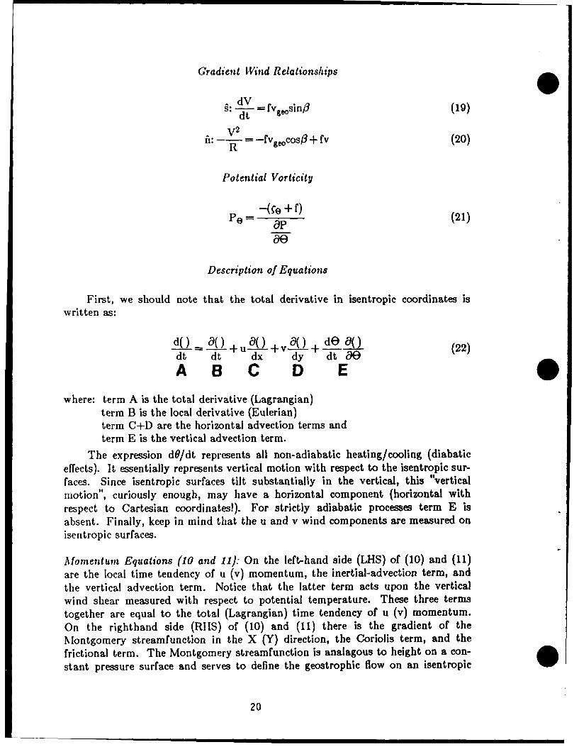
Gradient Wind Relationships

9: d__V _-v fgeosin# (19)dt

V 2

i: -R = -fv/gecso + fv (20)

Potential Vorticity

Po----e "( e + f) (21)

ae

Description of Equations

First, we should note that the total derivative in isentropic coordinates iswritten as:

d() o +uo() + () d () (22)

dt dt dx dy dt a(A B C D E

where: term A is the total derivative (Lagrangian)term B is the local derivative (Eulerian)term C+D are the horizontal advection terms andterm E is the vertical advection term.

The expression dO/dt represents all non-adiabatic heating/cooling (diabaticeffects). It essentially represents vertical motion with respect to the isentropic sur-faces. Since isentropic surfaces tilt substantially in the vertical, this "verticalmotion", curiously enough, may have a horizontal component (horizontal withrespect to Cartesian coordinates!). For strictly adiabatic processes term E isabsent. Finally, keep in mind that the u and v wind components are measured onisentropic surfaces.

Momentum Equations (10 and 11): On the left-hand side (LHS) of (10) and (11)are the local time tendency of u (v) momentum, the inertial-advection term, andthe vertical advection term. Notice that the latter term acts upon the verticalwind shear measured with respect to potential temperature. These three termstogether are equal to the total (Lagrangian) time tendency of u (v) momentum.On the righthand side (RIIS) of (10) and (11) there is the gradient of theMontgomery streamfunction in the X (Y) direction, the Coriolis term, and thefrictional term. The Montgomery streamfunction is analagous to height on a con-stant pressure surface and serves to define the geostrophic flow on an isentropic

20

surface.

[H/drostatic Equation (12): This is thp equation used to compute M on the isentro-pic surfaces. Iln pressure coordinates one integrates the hydrostatic equatiolia3P/(Z = -pg to obtain the hypsometric equation used to obtain heights on pres-sure surfaces. To do this it is necessary to integrate up from the earth's surfaceusing the temperature profile obtained by the rawinsonde. Similarly, here, oneobtains M by integrating (12) with respect to 0. Thus, the Montgomery stream-function consists of a thermal term (C T = enthalpy) and a geopotential energyterm (gZ) which are not independent tut related through the hydrostatic equa-tion.

.Mass Continuity Equation (18): This equation describes the change in massbetween two isentropic surfaces, as measured by AP, as a function of severalprocesses. One can also think of this expression as a static stability tendencyequation since 9P/O is the static stability. On the LHS there are the local timetendency and horizontal and vertical advection of stability terms. Together theyform the total derivative of stability which would be useful if one were followingparcels as in trajectory calculations.

On the RHS there are the divergence and diabatic terms. The divergenceterm changes stability in the following manner: divergence (convergence) in thelayer (AP) causes the isentropic surfaces to compact (separate) in the verticalthereby causing the stability of the column to increase (decrease). Thisshrinking/stretching of the column between two isentropic surfaces in response todivergence/convergence in the layer maintains mass continuity.

The diabatic term looks complex but can be described easily in physicalterms. Note that it is not just diabatic heating that is measured but its change inthe vertical. Thus, if the diabatic heating/cooling was uniform in the layer thisterm would be zero. However, let us say that there was diabatic cooling in lowerlevels due to evaporation and diabatic heating in upper levels due to latent heat-ing. Then, as seen in Figure 6, the static stability would increase with time.Essentially what happens is that in the presence of latent heating the 310 K sur-face is warmed to 314 K, meaning that the 310 K surface becomes redefined at ahigher pressure. At the same time the 305 K surface is being cooled to 301 K,redefining the 305 K surface to a lower pressure. The net result is to increase thestability as the two surfaces approach each other in the vertical. Other examplesof this nature could be shown depicting diurnal stability increases/decreases in thepresence of solar heating and terrestrial cooling processes.

Thermodynamic Equation (14): As Wilson (1985) notes, all adiabatic advectionand vertical motion is accounted for in the horizontal momentum equationsthrough M. The thermodynamic equation in isentropic coordinates states thatdiabatic heating (dQ/dt > 0) causes isentropic surfaces to propagate through theatmosphere in a direction toward l, wer potential temperature values. The expla-nation for this is that adding heat to a parcel will increase its potential tempera-ture (dlnO/dt > 0). Alternately, the surface in the presence of diabatic heating

21

310 * 310K "-

3 05 K : s 305

Figure 6. Schematic diagram depicting the stability changes that can take placein the presence of diabatic heating/cooling.

22

will become "redefined" at a lower level of the atmosphere. Conversely, in regionsof diabatic cooling isentropic surfaces propagate upwards towards higher potentialtemperature levels.

Montgomery Streamfunction (15). This expression states that the streamfunctionon an isentropic surface is the sum of the enthalpy, C T, and the geopotential atthat level. Again, these terms are related to each otlger through the hydrostaticequation (12).

Poisson's Equation (16): This equation is the founding expression for isentropiccoordinates. It enables one to compare parcels of air by computing the tempera-ture they would have if they were brought up (down) to 1000 mb--a base statelevel.

Geostrophic Wind Relationship (17): This expression relates the geostrophic windto the pattern of Montgomery streamfunction. The relationship is similar to thaton a constant pressure surface--the geostrophic wind blows parallel to theMontgomery streamfunction with lower values to the left of the wind (in thenorthern hemisphere). The geostrophic wind is also proportional to the gradientof Montgomery streamfunction and inversely proportional to the Coriolis parame-ter, f. One can create a geostrophic wind scale, similar to those used on constantpressure surfaces, which helps the analyst isopleth lines of constant M on an isen-tropic surface. Examples are given in Figures 7-8 for two different polar stereo-graphic scales (1:15 million and 1:10 million). To use them, place one point of acompass on one point on the Y axis at the latitude in question and the otherpoint to the right on the isotach value you want. The distance measured betweenthe goints is the distance two M lines should be apart (if drawn at intervals of 60x 10 ergs/gm) to support the given wind speed.

Thermal Wind Relationship (18): The thermal wind (the vertical shear of the geos-trophic wind) in isentropic coordinates is proportional to the mean pressure gra-dient in the layer. Since isobars on an isentropic surface are equivalent to isoth-erms, the thermal wind is also proportional to the mean temperature gradient inthe layer as is the case with pressure coordinates. The strength of the thermalwind is related to the vertical tilt of the isentropic surfaces, which is related to thepressure gradient recorded on them. The thermal wind "blows" parallel to themean isobars in the layer with low pressure (cold temperatures) on the left andhigh pressure (warm temperatures) on the right looking downwind. This diagnos-tic relationship is very useful in interpreting cross sectional analyses and will bediscussed in greater detail in Section 3.C.1.

Gradient Wind Relationships (19-20): The gradient wind equations are useful forstudying accelerated and curved flow. Equation (19) shows that acceleration(deceleration) takes place when the wind blows across the isopleths ofMontgomery streamfunction towards lower (higher) values, 3 > 0 (,8 < 0). Forgeostrophic flow 13 - 0 and there is no acceleration. Equation (20) describescurved flow as it includes the centrifugal force (term 1). For /3 = 0 it reduces to

23

00

cS

* %0

0 a$I~~ 4 00-

0 >)

L) * 0 0'

00 - Z4U(0 00 0

I J 0 0 w "

~1-4 P-1

C3 P4 00~40

0J U)

0004

4

c

tn

EElL* 0 o

00

10 0 0 0 C0

000 0 0 in 0 0) 0CO 1 ' -0 owl %n (. 1Xb0

24

000-4-4

:91-4

13. am41

z bob

00A44

41

UU

R 93 0 -

00 t.i~-4~) U 0to

04 00 0 b0&a0 00

~i 0

U 25

the standard gradient wind equation.

Potential Vorticity (21): Potential vorticity is defined as the ratio of the absolutevorticity, represented as + f, and the static stability in the column bounded bytwo isentropic surfaces. Under adiabatic, frictionless flow, potential vorticity isconserved, making it a useful "tag" for parcels. Reiter (1072) discusses how con-servation of potential vorticity can be used to trace air parcels out of the strato-sphere into the troposphere along tropopause "folds." Much of Danielsen's workreferenced earlier used this conservation principle. Holton (1972, p. 69-73) usesconservation of potential vorticity to describe lee side cyclogenesis. Under conser-vation of potential vorticity, if a layer bounded by two isentropic surfaces shrinks(stretches) in the vertical the absolute vorticity of the column must decrease(increase) in response. After an isentropic layer has crossed the Rocky Mountains,for example, it generally increases in depth as the lowest level follows the topogra-phy while the uppermost level remains relatively fixed, leading to increased vorti-city to the lee of the mountains.

F. Constructing an Isentropic Data Set from Rawinsonde Data

The isentropic analysis program that creates isentropic station data fromrawinsonde data came originally from a research program written for Danielsen'swork in the 1060's. The versions of this program used at St. Louis University(SLU) and by the Atmospheric Environment Service in Canada are nearly thesame. The total computation time to run the program on the University mini-computer is on the order of 5-10 minutes. Standard and significant level rawin-sonde data are needed. In the SLU version, wind data at constant height inter-vals (PPBB group) are used to interpolate winds to significant levels (TTBBgroup). This creates a complete sounding of pressure, height, temperature,dewpoint, wind direction, and wind speed for processing. The user can select theinterval between isentropic levels in the troposphere and stratosphere.

The actual procedures for the computation and interpolation of isentropicdata are described in Duquet (1964) and in Wilson, et al., (1980). Interpolation ofall variables except wind is done assuming linearity with respect to Pc where x =

R/C = 0.286. Winds are interpolated linearly with respect to height; directionand Rpeed are interpolated separately. Duquet (1964) notes that the latter methodof interpolation tends to smooth the wind hodograph. For each sounding the fol-lowing variables are computed at each isentropic level:

(1) Montgomery streamfunction (M) in units of 105 ergs/gm.

(2) Pressure (P) in millibars.

26

(3) Virtual Temperature (Tv) in degrees C.

(4) Height (Z) in gpm. The height is determined by integrating the hypsometricequation from the ground up.

(5) Actual specific humidity (q) in gm/kg. This is obtained by computing es (thesaturation vapor pressure) from the Clausius-Clapeyron equation using theinterpolated dew point temperature and then finding q from the relation:

.622e (23)P -. 378 e

(6) Saturation specific humidity (qs) in gm/kg. This is found as in (5) exceptusing the interpolated virtual temperature.

(7) Relative humidity in percent computed as the ratio of e/e s or q/qs.

(8) Wind speed and direction in degrees and m s 1 .

(9) Stability, upper and lower, measured as the distance in mb to the adjacenthigher and lower isentropic levels.

(10) Wind shear at a given level is determined from the winds and streamfunc-tions at the levels immediately above and below the isentropic surface. Direc-tions are given in degrees. Speed shears are multiplied by appropriate con-stants and displayed in millibars per degree latitude. These unusual unitsare useful to the analyst since they relate the vertical wind shear to the iso-baric gradient on an isentropic surface as discussed earlier in (18).

With respect to the Monetgomery streamfunction it should be noted thatwhen stated in units of 10 ergs/gm, a difference of one in the last digitcorresponds to a height difference of 1 meter. Therefore, a difference of 60 x toergs/gm, which is a typical contour interval for M, corresponds to 60 meters inheight on a constant pressure surface.

As noted earlier in the SLU version of the Duquet program, neutral-superadiabatic lapse rates will result in multiple pressure levels for one isentropicsurface. We prefer to average the variables for that level, applying them to amean pressure value instead of "adjusting" the sounding.

027

3. ISENTROPIC ANALYSIS TECHNIQUESIn this section we will explore various analysis procedures for both vertical

and "horizontal" plots of isentropic data. Emphasis will be placed on practicalapplications to everyday forecast problems.

There are basically three different charts used in isentropic analysis: the psichart, the sigma chart, and the isentropic cross section. The psi chart is namedafter ik, which typically represents a streamfunction--in this case the Montgomerystreamfunction. In this set of notes we have used M instead of V. The sigmachart is so named because static stability (W/90) is often represented as o. Itshould be noted that several researchers/analysts prefer to plot all their isentropicsurface data on one map rather than split it up into two charts. This is a user-selectable feature and therefore is left to the reader. For completeness we willshow several station models so that the reader may compare the various options.

A. Psi ChartsOn the psi chart the following variables are plotted: Montgomery stream-

function, wind direction and speed, mixing ratio, and relative humidity. The Mvalue can be plotted in cgs I r inks units. A typical value is 30,600 x 105 ergs/gmor equivalently 30,600 x 10 Joules/kg. Either way, the leading digit is usuallynot plotted-the 3 or 2 preceding it is understood. A typical station model plot isshown in Figure 9.

Contour intervals will vary according to the season but typical values forwarm/cold seasons are as follows:

Variable Contour Interval

Montgomery streamfunction 30/60 x 101 J/kgPressure 25/50 mb 1

Wind speed 10/20 m sAcutal specific humidity 2/1 gm/kg

Relative humidity 50/70/00%

As on any chart a maximum of three types of isopleths is suggested, prefer-ably using a color scheme along with solid, dashed, or dotted lines. The "startingvalue" of the Montgomery streamfunction is a function of the level. It is usuallybest to start at an even number; e.g. 31,000 or 20,800, whenever possible and, ofcourse, to be consistent from day to day on the same surface. The Montgomerystreamfunction field helps to define the flow of the geostrophic wind and also toidentify short/long wave activity much as on a constant pressure chart.

Isobars also should be started at some even number like 600 or 700 mb.They help to define cold and warm tongues on the isentropic surface. Strong gra-dients of pressure also can be used to locate frontal zones as seen in Figure 10.Anderson (1984) has described various isobar patterns in the vicinity of frontal

28

Montgomery streamfunction

in_ x 10 J/kg

Pressure (mb) -' 26 0600

relative humidity )1"0 1 . - specific humidity (gm/kg)

wind direction and speed (m/s) 2.- ten's digit of wind speed

Figure 9. Station model plot for psi charts.

29

P-3~/ j

P- 2 -/ <" N S i s

aw b

Figure 10. Isobaric topography in the vicinity of fronts (a) and isobaric topogra-phy associated with frontogenesis in the warm sector (b) (Namias, 1940).

6CO 5 0 55,6 5

6

70 07 5g

o

0

800/ 800 , 50"

Figure Ila. Isentropic pressure pattern in the vicinity of a strong, mature coldfront (Anderson, 1984).

30

systems. Figure Ila shows a pressure pattern in the vicinity of a strong maturecold front. The cold front is placed at, the leading edge of the pressure gradientwith the warm (high pressure) thermal ridge extending in a narrow tongue aheadof the front. Isobars are usually found to cross a frontal system undergoing fron-tolysis (Figure lib). The lack of structure in the pressure field is indicative of aweakening thermal gradient and decaying frontal zone. In the case of an occlud-ing system warm tongues tend to be diagnosed along the warm front and occlu-sion portions of the cyclone with a cold (low pressure) trough extending south-ward behind the cold/occluded fronts (Figure lc). Also, as discussed earlier, thecross-isobar component of the wind can be used qualitatively to estimate theupslope/downslope adiabatic vertical motion. Isobars are good as referencevalues, especially for someone just beginning iF'ntropic analysis and remind theanalyst of the three-dimensional nature of this "horizontal" surface.

Mixing ratio isopleths (isohumes) are, of course, essential for depictingmoist/dry tongues and their advection. Figure 12 depicts an idealized isohumepattern associated with an occluding system. It should be noted that in winter itis not uncommon to receive substantial precipitation out of clouds in which thespecific humidity is less than 1 gm/kg (Byers, 1938). Therefore, the isohume con-tour internal is seasonally dependent and level-dependent as specific humidityvalues often decrease rapidly with height. A typical isentropic upslope pattern isdepicted in Figure 13 with a south-southwesterly flow on this isentropic surfaceair being lifted as it transports moisture northward.

With two isentropic levels analyzed one can often diagnose regions where con-vective instability is being increased as dry air aloft is advected over moist airbelow. Such a situation is shown in Figure 14. Notice how low level moist air iscurrently being overlain by upper level dry air thereby increasing the convectiveinstability. In other cases it may be possible to predict this pattern bascd :;nadvection patterns at the two levels.

Relative humidity is helpful to estimate how close some areas are to satura-tion so that the analyst may be careful in interpretation. To avoid map clutterone may isopleth the 50, 70, 90% values or merely shade in green values exceeding70%.

Isotachs may be drawn as well to help diagnose jet streaks at low, middle, orhigh levels. Keep in mind that the jet streak depicted on an isentropic chart isbeing drawn in its three-dimensional detail so one is not only seeing its length andwidth, but its depth. One intangible benefit of such an analysis is that it rein-forces the view of the atmosphere as a continuous fluid. Such an appreciation isdifficult to obtain with constant pressure analyses, which are two-dimensional andquasi-horizontal.

B. Sigma ChartsThe sigma chart is primarily a stability chart. The variables typically plot-

ted on it are pressure, thermal wind, the number of millibars needed to reach the0 + 5K isentropic surface, and the number of millibars needed to reach the 0 - 5IC

31

front(Andeson, 084)

Figure 1 c. Isentropic pressure pattern in the vicinity of a frontal sys-

temn (Anderson, 184).

65

700

75

Figure I I c. Isentropc pressure pattern in the vicinity of a otlud ing o ld stemn (Anderson, 1984).

TOO32

Figure 12. Fronts indicated at the surface and schematic flow pattern around anoccluded cyclone as shown by the moisture lines in an isentropic surface in mid-air(Namias, 1040).

0 -0

IW M5 .. .. ." " ,.

I

-, /

Figure 13. Illustrating probable upslope motion of a moist current as deducedfrom the relation of the moisture lines to the isobars on an isentropic surface(Namias, 1040).

33,Se.. " (

.I s6 I 4 /Ms

Figure 14. Flow pattern at different isentropic surfaces which leads to increasingconvective instability. Solid (dashed) lines are isohumes at low (upper) level(Namias, 10)40).

33

isentropic surface. In this station model we have assumed that the 5K intervalwas chosen as an option when creating the data set. However, this numberdepends on the interval chosen, which is up to the researcher/analyst. The plot-ting model varies among researchers but looks essentially as shown in Figure 15.

Some people plot the total of the two LHS numbers in the bottom rightcorner, thus indicating the stability over a 10K interval. These numbers indicatethe static stability ( P/O0 ) which on a cross section would show up as the dis-tance in millibars between two adjacent isentropic surfaces. The greater the dis-tance between two adjacent isentropic surfaces, the greater the instability. Smalldistances between isentropic surfaces indicates great stability. In the stratosphere,for instance, the static stability is usually around 10K per 50 mb or less, whiletropospheric values are generally around 10K per 100-200 mb! By isoplething thetotal static stability (the sum of the LHS numbers) we can obtain an excellentdiagnosis of the instability.

Typical contour intervals will once again vary with the season but are typi-cally as follows:

Variable Contour Interval

Pressure 25/50 mbStatic Stability 10/20 mb

Although it might be better to analyze for the total static stability (lower AP +upper AP) it is good to see the breakdown of the two layers to see where thegreater instability is located.

The plotted thermal wind is computed for the layer surrounding the actualisentropic level in question. If one were analyzing the 300 K surface, the thermalwind would be valid for the 295-305 K layer (if a SK interval was chosen). Onecan use the thermal wind directions to help draw the isobars since, according to(18), the thermal wind over a layer "blows" parallel to the mean isobars of thelayer. Similarly, the gradient of the isobars can be qualitatively checked by not-ing the speed of the thermal wind. Strong (weak) thermal winds are associatedwith large (small) isobaric gradients on isentropic surfaces. One word ofwarning--these wind shears are based on the actual wind--not the geostrophicwind. So the degree to which this actual wind shear "obeys" the pressure gradientdepends on the degree to which the actual wind "obeys" the geostrophic wind. Itis possible for ageostrophic wind components; e.g., those in the vicinity of convec-tive systems or jet streaks, to produce wind shears which are out of balance withthe expected geostrophic shear. In any event, forecasters, especially those in avia-tion, should find these wind shear calculations informative for thediagnosis/prediction of turbulence. Other forecasters may use the wind shear tomeasure the significance of a frontal boundary or elevated inversion.

For completeness, we also show two other plotting models which essentiallycombine the features of the psi and sigma charts. Wilson (1985) uses the plottingmodel shown in Figure 16. He uses one variable that has not been discussed yet--

34

Number of mb needed to Pressure level ofreach 5K higher isentro- isentropic surface (mb)pic surface 7S uSfS

Number of mb needed toreach 5K lower isentro-,pic surface 6.-thermal wind (deg and mb/deg latitu

Figure 15. Station model plot for sigma charts.

35

Montgomery streamfunction stability - 111 mb be-

3049 x 10 2 J/kg tween this and next/ higher isentropic sfc.

wind speed 66 kt .... . .9 specific humidity (gm/kg)

Pressure 522 mb * 75*-..-saturation pressure

475 mb

Figure 16. Wilson (1085) station model plot.

CCC f pressure at condensation level PPP - pressure ofif lifted from isentropic surface i isentropiC surface

Ccc PPP

RRR = mixing ratio at isentropic surface observed wind closest to

(gm/kg/10) isentropic surface

Figure 17. Plotting model used by ISENT (NWS Southern Region isentropic plot-ting program used on AFOS), Little (1985).

36

the saturation pressure or lifted condensation pressure. Essentially this is thelevel to which the parcel must be lifted to achieve saturation. It gives a quickassessment of how close the atmosphere is to saturation at a station. More will besaid of this later. Other variables are as described earlier.

Little (1985) describes a program for AFOS called ISENT which plots isentro-pic data in the form shown in Figure 17.

As with any analysis scheme you should pick the station model(s) that suityour needs. The author usually tries to avoid analyzing more than three variablesper map-preferably only two for easier viewing and presentation.

C. Cross Section Analysis TechniquesWe now will turn our attention to vertical "slices" through the atmosphere-

cross sections. They usually are the first step in choosing the "horizontal" isentro-pic surfaces to analyze. One typically chooses the surfaces which are embedded inan interesting feature; e.g., baroclinic zones, jet streaks, or moist tongues. Gen-erally, in addition to the isentropes, it is also interesting to display mixing ratio(or specific humidity) and/or winds on the cross section. The mixing ratio profilesare useful in gauging the depth of the moist layer and possible areas of convectiveinstability (dry air over moist air). The wind profile is useful at depicting thevertical extent of jet streaks or wind maxima but also has an interesting relation-ship to the tilt of the isentropic surfaces. This is the subject of the next section.

1. Thermal Wind Relationship in Isentropic Coordinates

An isentropic cross section is generally chosen to be normal to a jet streak orwind maximum and therefore across a baroclinic zone (i.e., frontal zone). Thisallows one to depict the vertical and horizontal dimensions of the jet streak andattendant baroclinic zone. Mixing ratio profiles are also quite variable andinteresting in this area, too. Since the baroclinic zone is, by definition, a region ofstrong thermal contrast, one would expect to see a great tilt of the isentropic sur-face from high in the cold air to low in the warm air. From thermal wind con-sideration this requires strong vertical wind shear through these zones.

From our earlier discussion of the thermal wind you may recall that it"blows" parallel to the mean isobars in the layer or normal to the pressure gra-dient such that low (cold) pressure is to the left of the thermal wind lookingdownstream. In a cross section depiction we are graphically representing only acomponent of the total isobaric gradient. There is no guarantee that the chosencross section is exactly parallel to the isobaric gradient associated with the jetstreak. Therefore, we plot on the cross section only the wind components normalto the plane of the cross section. Wind components into the plane of the crosssection are generally designated as positive while those wind components out ofthe plane of the cross section are designated as negative. It is these normal windcomponents which have a relationship to the pressure gradients depicted in thecross section.

37

To obtain the normal wind components it is necessary to know the anglebetween the plane of the cross section and true north-south. However, rawinsondestations do not generally all lie on a straight line. So what is done? In the SLUcross section program we compute a least squares regression line for the stationschosen. The position of the stations is then chosen on this regression line perpen-dicular to the original station location as seen in Figure 18. One must intelli-gently choose stations which are approximately on a line because the regressionline computation is "dumb"; i.e., even a series of stations along a curve will beplaced on a line. Let the user beware!

Figure 19 is a schematic example of how we can relate vertical wind shear tothe tilt of isentropic surfaces in a cross section. Notice how the upper isentropicsurface slopes down from the cold air (pt. A) to the warmer air (pt. B). There-fore, the gradient of pressure in the plane of this cross section points from A to B.Since the thermal wind points in or out of the cross section with cold air to theleft (looking downwind), the thermal wind will point into the page in this case.The net result is that we expect the wind components into the page to increasewith height in this area of the cross section. This means that for this N-S crosssection westerly winds will increase with height. We can now state three generalrules:

(1) When isentropic surfaces slope down, the thermal wind is positive; i.e., windcomponents into the plane of the cross section increase with height.

(2) When isentropic surfaces slope up, the thermal wind is negative; i.e., windcomponents out of the plane of the cross section increase with height.

(3) When isentropic surfaces are horizontal (quasi-barotropic), the thermal windis approximately zero and the normal wind component does not change withheight.On a typical cross section one plots the potential temperature, specific humi-

dity and normal wihd components as shown in Figure 20.In the troposphere it is useful to draw isentropes at 2-4K intervals, but as

one nears the stratosphere it is best to double the interval to at least 4-8K as thestability is very strong. Since water vapor decreases quickly with height a goodcontour interval for specific humidity is 1-2 gm/kg. Finally, isotachs can bedrawn at 5 m/s intervals. Remember that values can be + or -; therefore, a zeroline may need to be drawn.

2. Isentropic Topography in the Vicinity of Upper-Level Frontsand Jet Streaks

An averaged, idealized cross section from north to south is shown in Figure21. There are many interesting features in this cross-section. They include:

38

AaB C

CD

c deE regression line

Figure 18. Schematic showing how stations are depicted with respect to theregression line and their original positions.

039

200

oo-__

7175'72.5 72g461741 2

Figure 19. Cross section illustrating the relationship between sloping isentropicsurfaces and the vertical wind shear. Solid lines are isentropes and dashed linesare normal wind components where + (-) indicates winds into (out of) the plane ofthe cross section.

040

Potential Temperature ( K)-)032 .~/. specific humidity (gm/kg)

+ ~ normal wind component (m/s)

Figure 20. Cross section plotting model.

41

20 Jo ~m t S0 Kt.

20-

too

90 0 S •30 So

Auum sesn.I umrtetoppi it tmdl and, high.. + l attds

(FJ)rea oftIeaied nd eragedththeurea rtespecialye ovr the ontinns thegAditin he roosphumer are strongaer t adth saidlit isd hgreaterdbutnhoshera asrsablent as the rther Then opingnishoe impl thateasoi

westerlies increase with height in the troposphere, and decrease with height tobecome easterlies in the stratosphere, except at very high latitudes. There is againa strong seasonal variation in the stratosphere, with westerlies at high latitudesmoving southward to middle latitudes and strengthening in winter.

42

. . .ii l

(A) The polar frontal jet (PFJ) and its associated polar front are seen around40-50 N. The polar front is depicted as a sloping zone (indicating strongthermal contrast) and as a compacted isentrope zone indicating stability.Although it is shown in Figure 21 as identifiable all the way to the surface,this is not alwayb the case, since the isentropic surfaces lost continuity in theboundary layer. The PFJ is placed at about 350 mb, a little lower in theatmosphere than perhaps it should be. It is above the polar front where thevertically-integrated result of the thermal wind effects is greatest. Note howthe isentropes slope up above the PFJ, indicating a reversal of the thermalwind in the stratosphere and a subsequent decrease in westerly momentum.Also notice how there is a gap in the tropopause in the vicinity of the PFJ.In fact the polar front appears as an extension of the strongly stable air ofthe stratosphere. In this region there is considerable stratospheric-tropospheric air exchange. This shows that the tropopause is not quite the'lid" or impermeable layer it was once thought to be. We will return to thisconcept later.

(B) The air in the troposphere is much less stable than the stratospheric air.This is seen by comparing the vertical distances between isentropes in bothregions. The air in the troposphere is not unstable generally but relativelyless stable --the farther apart the isentropes the less stable the lapse rate.Potential temperature lapse rates of 10 K/100 mb are not uncommon,whereas in the stratosphere lapse rates are generally about 10 K/50 mb ormore.

(C) The arctic front shows up as a shallow, few kilometer deep layer of stable airwith strong vertical tilt. This is a good example of how one can gauge thedepth of systems and perhaps, as in this case, determine whether a system inlow levels is vertically coupled to the upper air flow.

(D) The subtropical jet (STJ) is shown to be associated with a weak upper tro-pospheric front. This is not unexpected since the STJ is not explainedthrough thermal wind arguments as is the PFJ. It comes about as a result ofair flowing north in the upper branch of the Hadley cell circulation attempt-ing to conserve its angular momentum. As it flows north its angular velocityincreases in response to a shorter distance to the earth's axis of turning. TheSTJ can be even stronger than the PFJ, with speeds of up to 260 knotsobserved over Southern Japan (Palmen and Newton, 1969). Palmen andNewton (1969) also observed that the STJ is characterized by great steadinessin both wind direction and geographic location, and tends to have an anticy-clonic curvature. The STJ tends to be associated with a "break" between themid-latitude tropopause at around 250 mb (noticeably higher than the PFJ)and the tropical tropopause typically found at 100 mb. Often on jet chartsor 200 mb charts it is difficult to determine if a jet streak is part of the PFJor STJ. A cross section of winds will help diagnose these two jet streams.However, in the winter it is not uncommon for the two jet systems to merge

43

as the PFJ moves southward with the polar front.

(E) The tropopause, especially in middle and higher latitudes, is easy to locate,except near significant jet streaks where the tropopause "breaks" occur. Thetropopause appears as a zone where the vertical lapse rate of potential tem-perature increases by about an order of magnitude.

D. Useful Diagnostic Variables Computed from Isentropic DataOnce an isentropic data set has been generated from rawinsonde data it is

relatively straightforward to interpolate the station data to a grid on a map pro-jection (e.g., lambert conformal, polar stereographic). This can be done using oneof the more popular objective analysis schemes (e.g., Barnes, 1973). Details of thisprocedure will not be discussed in this paper. For an excellent treatment of thissubject see KCoch, et al., (1983). Once grids of u, v, P, q, M are obtained for aparticular isentropic surface numerous diagnostic variables may be computed. Inthis section we will briefly discuss some of these variables and how they might beused in diagnostic analysis.

1) Static Stability: This variable can be expressed as AP = P (upper 0 surface) -P (lower 0 surface) which is always <0, although some people like to define it inthe opposite sense so that it is always > 0. In any event, it is a relative measureof instability which does not take moisture into account. Horizontal plots of thisvariable on an isentropic surface, using adjacent surfaces for the computation, V e"quick and dirty" estimates of stability and stability change. Units are millibars.

2) Moisture Advection/Convergence: Moisture advection is expressed mathemati-cally as -V.Vq. Values > 0 (or < 0) indicate increasing (or decreasing) moisturelocally. Local increases or decreases of moisture; e.g., through evaporation or con-densation, are neglected. Essentially it evaluates quantitatively what one can esti-mate qualitatively by superimposing the flow (streamlines or Montgomery stream-function) over the isohumes. Units are generally gm/kg-hr x 10. Multiplying by10 inflates the values to bring out important features.

To take this one step further, one can compute moisture convergence on isen-tropic surfaces expressed as -. qV=-V.Vq-q.V. As you can see, it includesthe advection of moisture and the effect of divergence/convergence on the moisturefield. In an isentropic framework this variable measures not only the advection ofmoisture but also the destabilization (or stabilization) that takes place with con-vergence (or divergence). Thus, positive values indicate positive moisture advec-tion and/or destabilization due to convergence. This is often useful in forecastingconvection. Negative values indicate drying out due to negative moisture advec-tion and/or stabilization associated with divergence. Units are gm/kg-hr x 10.

3) Adiabatic Vertical Motion: This variable can be expressed as:

44

WadJabatic V 'Ve P

N, gative (positive) values imply upward (downward) motion on an isentropic sur-face This expression is a reasonable approximation to (7) since, as described byHoman and Uccellini (1987), the local pressure tendency term will always actagainst the diabatic term in (7). The remaining term shown above is thus a goodapproximation to vertical motion, especially at the synoptic scale. It is essentiallymeasuring what you would qualitatively estimate from the cross-isobar componentof the streamlines or Montgomery streamfunction. Units are generally Abars/secto be consistent with standard measures of vertical motion.

4) Static Stability Tendency: This variable is taken from the continuity equation(13) discussed earlier. Assuming no diabatic effects we can write (13) as:

Since 81P/19 is always < 0 (for 9 to be a valid coordinate!) it flips the sign of thetendency term. If either the advection or the divergence term is negative they con-tribute to destabilization. Likewise, positive values indicate a tendency towardsstabilization. The advection term simply moves existing patterns of static stabil-ity about, while the divergence term can create or destroy static stability. Diver-gence in the layer acts to increase stability (+ sign) while convergence acts todecrease stability. To compute these terms one uses o/a9 centered on the isen-tropic surface whose u and v wind components are used. Units can be written asmb/K-s x 10- 5 .

5) Absolute Vorticity: Absolute vorticity can be computed as:

Ore 8 ue

ie7 - e +f---- a y f (25)

using u and v wind components on an isentropic surface. Absolute vorticity is

one of the most basic variables used for analysis in synoptic meteorology. Vorti-

city is useful in diagnosing short waves and their intensity, the same as on iso-

baric surfaces. It is especially helpful in depicting strong horizogtal1 shear zones

associated with westerly jets with little curvature. Units are x 10 s .

6) Potential Vorticity: This variable is written as shown in equation (21):

P -(e+ f)4P

45

Potential vorticity is useful as a tracer for atmospheric flow under adiabatic,frictionless conditions. It can be especially useful, when interpolated to cross sec-tions, to diagnose the intrusion of stratospheric air which generally has potentialvorticity values about one order of magnitude greater than tropospheric values(Reicer, 1972). When air extruding into the troposphere along the polar frontexperiences convergence, it increases its cyclonic spin in an effort to conserve itspotential vorticity. Staley (1960) notes that the potential vorticity of a parcel ischanged only by diabatic heating and/or friction. Units are typically cm-s-K/gmx 10-O .

7) Condensation Pressure: This variable was first suggested by Byers (1938) tohelp better represent moisture on isentropic surfaces. It is simply defined as thepressure to which unsaturated air must be raised dry-adiabatically in order toreach saturation; i.e., the condensation level. It is typically expressed in millibars.The key advantage of condensation pressure over specific humidity is that conden-sation pressure better represents moisture differences at low values of q. This canbe seen best in Figure 22, which presents condensation pressures vs. specific humi-dity for various potential temperatures. Note that along each isentropic surfacethe slope ( a)P/,9q )0 is greatest at low values of q. Byers (1938) notes that on anisentropic surface a specific humidity between 1 and 0.5 gm/kg is poorlyrepresented, while condensation pressure isobars make it stand out about as muchas a 5-10 gm/kg difference. This is important, especially in winter when lowspecific humidity values are often associated with significant precipitation andclouds. Simple algorithms are available to compute the condensation pressures forunsaturated air.

Anderson (1984) notes that condensation pressure isobars can be useful inidentifying frontal positions. A moist tongue, represented as a ridge of condensa-tion pressure is usually present along or slightly ahead of a strong, mature coldfront (Figure 23a). As a cyclone occludes the moist tongue will typically branchinto two tongues--one turning cyclonically to the northwest and the other anticy-

clonically to the northeast. The occlusion is usually found in the vicinity of thebranching (Figure 23b). Anderson (1984) notes that the precipitation is oftenheaviest in this area.

8) Condensation Ratio: Byers (1938) defines this variable as the ratio of the con-densation pressure (Po) and the actual pressure (P) of a point on an isentropicsurface. It is a measure of nearness to condensation and is dimensionless. Con-densation ratio can then replace relative humidity on the psi chart.

Byers (1938) points out that nearness to condensation can also be estimatedby the distance between an isobar (P) and an isobar of condensation pressure (Po)

having the same value. If the prevailing flow is expected to move a Po isobar overa P isobar of the same value, saturation and precipitation can be expected.

9) Condensation Difference: Anderson (1984) notes that the condensation ratio is

not easy to analyze. He suggests computing the condensation difference by sub-

tracting the value of the condensation pressure from the corresponding pressure

46

400

oo

47

0 ,, 4 6 a II 0 a ii

50

500

6005O

65O

.6506 5

Figure 23a. Isentropic condensation pressure pattern over a mature, strong coldfront (Anderson, 1984).

4504

soo

Figure 23b. Isentropic condensation Pressure pattern over an occluding frontal

system (Anderson, 1984).

48

value on an isentropic surface. The smaller the value of the condensationdifference, the closer the parcel to saturation. Due to smoothing and round-offerrors, a difference of less than 20 mb represents saturation. For summer over thewestern U. S. he found values < 100 mb to be useful indications of near-saturation.

Edson (1966) discusses the use of the "condensation pressure spread" for cloudforecasting. Figure 24 is his diagram illustrating the relationship of this variableto cloud cover for various pressure levels.

10) Streamlines: On the CSIS system and the isentropic program designed byAnderson (1984), a streamline analysis is available for display, usually to overlaywith one other variable. Streamlines, it should be remembered are based on theactual wind and display the instantaneous field of motion. They can be overlaidwith the Montgomery streamfunction to depict regions of ageostrophic flow .They also are excellent for depicting regions of convergence/divergence which, inan isentropic framework, are associated with destabilization/stabilization. How-ever, they do not display any speed information. So, although streamlines cross-ing isobars, for instance, generally imply vertical motion, one cannot get a quanti-tative measure of omega from such a field.

Anderson (1984) states that streamlines will tend to converge in the vicinityof frontal boundaries (Figure 25a), especially in regions of frontogenesis. Whenstreamlines flow across a front as depicted in Figure 25b the front is weak and inthe process of frontolysis.

49

0

10 I 0 me

40. ?0

Ida

2

Figure 24. Condensation- pressure spread to cloud-conversion table (Edson, 1966).

50

Figure 25a. Isentropic streamlines in the vicinity of a strengthening cold front(Anderson, 1984).

Figure 25b. Isentropic streamlines in the vicinity of a weakening cold front(Anderson, 1984).

51

4. SPECIALIZED APPLICATIONS OF ISENTROPIC ANALYSESTO DIAGNOSTIC/FORECAST PROBLEMS.

There have been numerous applications of isentropic analysis techniques tothe study of extratropical systems and, more recently, to mesoscale systems. Inthis section we will briefly describe some of these applications, referring the readerto the original papers for a more in-depth treatment of each approach.

A. Isentropic Trajectories

There are two basic approaches to computing trajectories on an isentropicsurface (Dutton, 1976):

1. If the equations of motion are solved on a gridwith fine resolution, then trajectories can becomputed for any parcel by geometrical methods.This is known as the explicit method.

2. If a sufficient number of conservation propertiesof an air parcel can be identified, then we canobserve their values in a parcel at one time andthen find the parcel's new location at a later timeby finding where the same combination of values ofthese variables occurs.This is known as the implicit approach.

1. Implicit Approach

Danielsen (1961) outlined the implicit approach of computing isentropic tra-jectories which is based on a total energy equation.

We begin with the two dimensional inviscid equations of motion in isentropiccoordinates:

dV _-M - fxv (26)dt

Dotting (26) with V yields:

d [V2(27)

Next, we write the total derivative of M assuming adiabatic conditions

d =-+VVM (28)idt ot

52

Solving for the advection term in (28) and substituting into (27) results in:

(22dM +V_1 am (29)

This is an energy relationship which can be applied to a parcel trajectory byintegrating (29) over time, resulting in:

Mf-M1 +~(~ -Vf = -- " 2 dt (30)

The RHS term of (30) can be approximated at the initial (i), midpoint (m) andfinal (f) points of the trajectory and weighting the midpoint, i.e.,

tvam i + 2Am+AM=M "+t +4 (31)

resulting in a finite difference form of the integrated energy relationship:

Mf-Mi+V (V2-V 2). M i + 2m " (32)4

This relationship and a distance formula written as:

D i+V A (33)2

can be used to construct a trajectory. Essentially, the energy relationship (32)and the distance formula (33) must be solved simultaneously by choosing a pointon an initial isentropic surface at a certain time, and then exploring the down-stream area on the same isentropic level X hours later (usually 12) which balancesboth equations. This can be done graphically but is quite laborious, even thoughDanielsen's early work was done this way (Danielsen, 1066). Later on this processwas adapted to a computer as described by Danielsen and Bleck (1967) andHaagenson and Shapiro (1070).

Figure 26a displays the initial time period on the 328 K isentropic surfaceused in a study by Danielsen and Reiter (1960) for trajectory calculations. Theisentropic trajectory is plotted in Figure 2Gb to display the same surface 12 hourslater over the central U. S. Notice how a trajectory, initially located on the anti-cyclonic side of the jet streak, turns towards higher values of M and descendsfrom approximately 370 mb to 460 mb while slowing down enroute. Its path

53

31.1202032 33 3135

30020 3120~ 312 335=3 3296

3154*34

0(0'dgS 0.4 MOW.315

2 35 4" POc

Figure16,4 265. Isnroi srac,0 45,030GM Jnay g.Nmeiavalues17 to the lef of eac s2aio indcat prssr 316an0pcii umdt

(M). ~ ~ ~ ~ 0 Isl2e ofMae aeedi1niso 1 (ails ad11tr,16)

25348

3170-423'71 6

/ E, \337 4gS 4003180 4 46~. 076k

10.30 10.11 3164230 670

3100-t4os :037

Figur 28b Isetropc suface 3=4561 C,15 0.0T8Jaur715. Trjctores re hon fr te imeperod0301 0 GMT onta da.Th3pra

betwee th<w0rjcore.losfr2ncuaisinwn eot (aile n

55I r38

agrees well with the "digging" trough into the central U. S.

2. Explicit Approach

Petersen and Uccellini (1979) note that there are some problems with theimplicit approach. The simultaneous solution of (32) and (33) for anticyclonictrajectories does not always converge to a unique solution. Secondly, the estima-tion of the local derivative term (RHS term of (32)) is only fair, at best, for the12-hour time interval imposed by operational data availability. The basic tech-nique applied to (32) and (33) makes it difficult to account for varying accelera-tions that take place along the trajectory. The explicit technique of constructingisentropic trajectories provides a better alternative that is easier to code up for acomputer.

To begin with, one needs to have gridded values of u and v wind componentsfor the initial time period and M values for both the initial and final time periods.Next, we compute the accelerations in x and y space from the invisicid equationsof motion in isentropic coordinates; i.e.,

Au AMAu = -M + fv (34)At Ax

Av= AM fu (35)At Ay

using standard finite difference techniques to compute the M derivatives. Then wecompute the new u and v velocities for the parcels with

u -=u° + At (36)At

v +AVAt (37)

which are "starter" formulas used for the first time increment, A t. Superscriptsrefer to the time step. For other than the first time step we use,

ut+l= ut +At [ At 1 Aut-1 (38)t At]

vt+ I vt +At 3 1. Av-'1 (3g)[2 At 2 AtJ

56

Finally, we compute the new position of the parcel with

xt+ x t + (ut+l + ut) (40)

y t+ _ yt + YAt(vt+ 1 I vt) (41)

A time step of 15-30 minutes is typically used. An M field is needed for each timestep. This is done by linearly interpolating in time between the two M fields.Also, for each iteration in time one needs M derivatives in x and y space interpo-lated to the parcel location. One typically computes these derivatives at gridpoints and interpolates them to the parcel location. It is important that theinterpolation scheme be accurate. Petersen and Uccellini (1979) used an overlap-ping polynomial technique which they describe in their paper.

The application of this explicit technique is very straightforward and yieldstrajectories which are nearly energy-conservative. If one has gridded fields of u, v,P, q and M for both time periods, it is possible to compute change fields followingthe parcel as well as keep track of the parcel's relative humidity. This enablesyou to quantitatively determine how long to "trust" the parcel trajectory, perhapseven terminating it upon saturation.

Figures 27 a-b show the isentropic charts and trajectories derived from theexplicit approach from a study by Petersen and Uccellini (1979). Note how wellthese trajectories follow the flow.

3. Trajectory-Derived Variables

Once a trajectory has been calculated, it can be informative to producechange fields based on the trajectory's initial and final points. Changes inenthalpy, internal energy, potential energy, kinetic energy, pressure, and potentialvorticity can be computed by using these variables' values at the end points of theparcel and plotting the "delta" value at the parcel's spatial midpoint. If enoughcalculations are done in this way, one can then analyze this Lagrangian-derived,irregular set of data. Much information concerning the thermodynamics anddynamics of the atmosphere can be learned in this way.

Consider the following information from an isentropic trajectory:

0 = 305 K 12 hour changes

M initial = 30500 x 105 ergs/gm M final = 30560 x 105 ergs/mg

P initial - 250 mb P final = 500 mb

V initial -50 m s " V final 30 m s -1

From this information we can calculate the following "delta" values:

57

NIN

2300M 25193k. * 2

Fiue 2a630 K snrpcsufc6o3 20 M ~M 2 .n 00G T1

windGM report97 (Ptese and UceIii 1979).97

200208

I ......... ..

. . . . . . .. .I ...... ..

001

.. .. . ...

- - .1 n _ L.... . . ...

Figure 27b. Trajectories computed for 1200 GMT 10 May through 0000 GMT 11May 1973 on the 330 K isentropic surface using discrete model technique. Posi-tions at 3 hour intervals are indicated by the solid black dot. The Iinitial andfinal wind direction and speed are indicated (31426 == 314 0, 26 in s1 (Petersenand Uccellini, 1979).

59

A Enthalpy = + 45 x 10 7 ergs/gm since A T = + 45 K

A Internal Energy = + 32.25 x 107 ergs/gm

A Potential Energy = - 45.38 x 107 ergs/gm

since A M = +0.6 x 107 ergs/gm

A Kinetic Energy = -0.8 x 107 ergs/gm

w = AP/At = + 5.79 P bars/s

At a glance we can see that this parcel warmed 45K as it descended 250 mb adia-batically, thereby increasing its enthalpy and internal energy while decreasing itspotential and kinetic energies as it "crossed over" to higher M values. Note thatthe kinetic energy change is about an order of magnitude less than the otherchanges. The descent rate of + 5.70 p bars/s is substantial for the synoptic scale.

Rubino (1986) has computed various change fields for isentropic trajectoriesduring the Atmospheric Variability Experiment-Severe Environmental Storms andMesoscale Experiment (AVE-SESAME) I period, 1200 GMT 10-11 April 1979. Fig-ures 28 a-c display several trajectory change fields during AVE-SESAME I for the312 K surface (see Figure 31a for radar summary).

B. Potential Vorticity and Tropopause Folding

It is difficult to do justice to this topic in this paper. The goal of this sectionis to simply acquaint the reader with some of the past and present work withrespect to the topic of stratospheric extrusions or tropopause "folds". For anexcellent. rview of this topic the reader is urged to read Keyser and Shapiro(1086).

As routine upper air soundings became available and the vertical temperaturestructure of the atmosphere began to be diagnosed, the concept of a tropopause"lid" capping the troposphere became entrenched in meteorc!ogical terminology.This natural inversion above the "weather sphere" appeared to preclude any verti-cal transport of mass between the troposphere and stratosphere. Secondly, asReiter (1972) notes, "Isobaric thinking" led to the acceptance of a jet axis asrepresenting a discontinuity of absolute and potential vorticity. This made itdifficult to envision how air masses could cross the jet axis under conservation ofeither of those two quantities. Therefore, the jet axis was thought to be a barrierto lateral exchange processes.

However, from the mid 1050's to this day much research documentation hasshown a substantial mass exchange between the stratosphere and tropospherealong tropopause "folds" or "breaks" (see Reed, 1955; Staley, 1960; Danielsen,1968; Reiter, 1972, 1975; Shapiro, 1980; Uccellini, et al., 1985). Several of theseauthors used stratospheric tracers of ozone, radioactivity, and potential vorticityto document airflow into the troposphere. Air descending from the stratosphere

60

II

- _-_. ..

I_- . l 1..r/ ,''"- - I .. - "

I / ; ,i

I-"- .., .. . . -

I /" I

I S

Figure 28a. 312 IC 3-hour isentropic trajectories beginning 1700 GMT 10 April I

I "\ ("S

I -r'~ / /

I1 (-'.s '• -- \•I I

r - I I . . - I', - _ ' -

I -.. " .. . .. 'SS .. . . ; ,

Fiur-2b-31 K3-ou-dlt field for 17020 GM 10Arl17(Ruin, 186. Uit ar Jkg 1I ! .is # # II I o"61

I II

I \("

- I I5

I --,S '-.. .. . I~- -- I- - -

/ I -

-I

, "ia I

I \

, i L ,

Figure 28c. 312 I( 3-hour vei c l m t o fi l f r 17 0 2 0 M l0 A il 1 9(R'n,1 8 ) n1 t ar 0icrob ars/s

\~0'~57 62

is also characteristically "bone dry" (i.e., RH < 10%).

Figures 29 a-f display a synoptic situation during which a tropopause foldformed. The top three panels (Figure 29 a,c,e) show the rapid deepening of a amid-tropospheric wave over the central U. S. from 0300 GMT 13 December to0300 GMT 15 December 1053. Note the intensification of the thermal gradientattendant with the developing jet streak at 500 mb. By the end of the period ahyperbaroclinic zone is established along the east coast, with wind speeds exceed-ing 150 knots. Cross sections taken perpendicular to the jet (Figure 29 b,d,f)diagnose the development of the tropopause fold. The strong static stability andnegative wind shear help to define the stratospheric air. The tropopause is lowestwhere the air is coldest in the mid-troposphere. Stratospheric air sinks over thefirst 24-hour period and then finally extrudes into the troposphere by the last timeperiod (Figure 29f). The stable baroclinic zone associated with the strong frontalzone is defined by both highly compacted isentropic surfaces and strong verticalwind shear. The vertical shear of the geostrophic wind is nearly zero in thoseareas outside the frontal zone where the isentropic surfaces are quasi-horizontal.

Uccellini, et al., (1085) have documented a tropopause fold that took placeduring the President's Day Cyclone of 18-19 February 1079. From a forecaster'sviewpoint, what is most interesting about their study is how they correlate a foldin the tropopause to subsequent explosive cyclogenesis for this east coast storm.A key diagram from their study is shown in Figure 30 a-d. In the last diagramone can identify a stratospheric extrusion from the stable baroclinic zone descend-ing from Peoria, IL (PIA) to Appalachicola, FL (AQQ) and the high potential vor-ticity values along the frontal zone. Uccellini, et al., (1985) show that stratos-pheric air descended along this zone at least 12 hours preceding cyclogenesis. Itmoved down to - 800 mb toward the east coast to an area upstream of whererapid cyclogenesis occurred. There, it experienced adiabatic mass convergence andin an effort to quasi-conserve potential vorticity vertically stretched and increasedits absolute vorticity. Their work is further substantiated by ozone measurementsfrom the Total Ozone Mapping Spectrometer (TOMS) flown aboard the Nimbus 7satellite. TOMS measures the vertical ozone distribution in the stratosphere. Amaximum in ozone concentration is positively correlated with a relatively thickstratosphere and a thin troposphere. They have shown significant positiveincreases in TOMS ozone measurements in the vicinity of these tropopause folds.Shapiro, et al., (1982) have used the TOMS in a similar application to show howozone maps from TOMS can locate jet streaks at tropopause levels and guagetheir intensity from the intensity of the gradient of the ozone distribution. Thiscould be a useful technique for locating jet streak activity over data sparse regionsand approximating their magnitudes.

Utilizing isentropic cross sections with mixing ratio, normal wind componentsand potential vorticity in the operational setting may provide clues to timing theintensity and onset of significant winter storms. The author's experience is thattropopause folds are more typical with the stronger systems (central pressure<990 mb) during the cold season. The practical application of this technique isyet to be proven--but the potential exists and the data can be computed in real-time.

63

.20w

24

amwo

-soo

.12.

'00 ___W____So

30 3.

640

72 no0

to

• --840

Non

CIO, No

~00

INo

,.'r .- -f - d-

...

-l

1k III M

Figure 29d. Cross section along line C-D in Figure 20c. Heavy dashed linesrepresent boundaries of stable air; otherwise notation same as in Figure 29b(Reed, 1955). 65

X- I =.Ift

720

760 jh'9112760

a- .24

.2 000840

-~ ' ' '~ Sb/Goo.Ago

'-to

40. 92

Figure 29e. 500 mb surface for 0300 GMT 15 December 1053. Heavy solid linesrepresent boundaries of frontal zone (Reed, 1055).

-4 F.

Figur 2.Cosscinaog ieEFi0iue2e Ntto aea nFg

ur 2b nd29 (ee, 05)

66A

A 1200 GMT 18 FESB79 1 200 GMT 18 FESI

__ _150 15

eL. 71- 200 200w

O,6 300 300 12

9400 400 f-I

2' ~40 5W500- 0 101

'-130 10

600 700 223~

850 6C 1~7

1000 100072747 265 75472747 72655 72654 72562 72765 764 72562 72469 INL STC MON L16FDINI STC MON LBF DEN

Figure 30a-b. Vertical cross section from International Falls, MN (INL) toDenver, CO (DEN) for 1200 GMT 18 February 1g7g. The left panel (A) is an iso-tach analysis for total wind speed (m s-1 ); wind barbs plotted with last digit ofwind observation. 1 The right panel (B) shows isentropes (solid, K); geostrophicwind (dashed, m s- ) computed from the horizontal thermal gradient in the planeof the cross sectin; potential vorticity, -( + f)/(a0/8P), heavy solid, where 10=10 x IT" IK mb- s- Potential vorticity analysis is only shown for upper portionof frontal zone and stratosphere (Uccellini, et al., 1085).

67

L00 COOGMT19 FES 79 d00 M 9FS

£ 'I 60< ,300 30

40400 .1

3030

617 60 60

:1 650 8502

W265 72532 72433 72327 72229 72220 1UIA JEGAS PIA SLO SNA CKL AOO 724 72S32 72433 72327 72229 72220

GAS PIA SLO DNA CKL AQO

Figure 30c-d. Vertical cross sections from Green Bay, WI (GRB) to Apalachicola,FL (AQQ) for 0000 GMT 19 February 1979. Depictions same as in Figure 30a-b(Uccellini, et al., 1985).

68

C. Short Term Forecasting of Severe Convection Using IsentropicAnalysis

Although isentropic analysis is best suited to cold season eases ofcyclogenesis/frontogenesis when horizontal thermal gradients are most distinct inmid-latitudes, several authors have suggested its use in the short term forecastingof severe convection. Namias (1038) was probably the first researcher to promoteusing isentropic charts as an aid in thunderstorm forecasting. He emphasized theuse of cross sections of potential temperature and specific humidity and '!horizon-tal" isentropic analyses as useful charts in diagnosing and anticipating moisturepatterns. He noted that, "tongues of dry and moist air may be followed from dayto day by means of these charts, for it is reasonable to suppose that the majoratmospheric motions are approximately adiabatic." This is especially true in thepre-convective environment before the onset of strong solar and latent heating.

More recently Wilson, et al., (1980) and Moore (1085) have described analysisprocedures on isentropic charts which can help forecasters diagnose severe convec-tive threat areas on meso alpha scales of motion. Wilson, et al., (1980) con-structed a four panel chart consisting of:

(1) one panel with only station models as described in Figure 16,

(2) one panel with isopleths of Montgomery streamfunction and pressure,

(3) one panel with isopleths of Montgomery streamfunction and stability, and

(4) one panel with isopleths of Montgomery streamfunction and specific humidity.

A mid-level isentropic surface is chosen to help depict upward/downwardvertical motion, moist/dry tongues, moisture advection, and stability. An upperlevel isentropic surface is chosen to diagnose jet streaks, their strength, curvature,and proximity to the possible threat area. These two isentropic surfaces may bechosen by using climatological average values or by consulting a cross section withnormal wind components and specific humidity superimposed. On the mid-levelisentropic surface, a dry line can be defined as the inner moisture isopleth on thedry side of the gradient while the moist tongue is taken to be the zero moistureadvection line according to the M and q analysis. On the upper level isentropicsurface, jet streaks are defined according to the actual wind field and the orienta-tion and gradient of the Montgomery streamfunction.

A depiction chart (similar to a composite chart) is prepared by placing thesurface front, dry line, moist tongue, and the middle and upper-level jet streakpositions on one chart. Although the authors do not mention it, one could easilyadd the axis (or axes) of greatest instability as well. Forecast positions of thesefeatures are placed on the chart, as well. The forecast position of the surfacefront is taken from forecast charts while moist tongues and dry lines are forecastusing 100% of the wind speed at the lower isentropic level. Jet streak positionsare subjectively forecast from prognostic charts, showing continuity and relation-ship to the surface front. The authors then place the maximum threat area aswest of the mid-level dry line and east of the surface front, and near the mid-level

69

jet streak. Typically the strongest convection takes place to the right (lookingdownstream) of the mid-level jet streak. Greatest destabilization takes placebetween the mid-level moisture maximum and the dry line. Since this region usu-ally has ample low level moisture it is an area of strong convective instability.

As a follow-up to the previous study, Moore (1985) expanded on the conceptspresented by the above authors. He developed five diagnostic charts based onisentropic surface data. They include charts depicting:

(1) Montgomery streamfunction isopleths and isobars,(2) Adiabatic vertical motion isopleths and isohumes (specific humidity),(3) Horizontal moisture convergence field and low level static stability,(4) Low level stability flux field, and(5) A composite of key features--pressure ridges, upper level jet axis, and

centers of upward vertical motion, minimum stability, moisture convergence,and stability flux convergence.

In his study Moore found that the threat area for AVE-SESAME I was character-ized by:

(1) thermal riding (pressure axis);(2) relatively low static stability;(3) proximity to a moist axis;(4) proximity to a moisture convergence maximum;(5) strong adiabatic upward vertical motion;(6) strong positive stability flux (destabilization) and,(7) being along the upper level jet axis, preferentially in the exit region.

The charts used in this study are shown in Figure 31a-g. Figure 31b shows thecross section used to choose the representative isentropic surfaces. Figures 31c-gare the charts described above. Note how the juxtaposition of the key thermo-and hydrodynamic features described above help depict the strong convection 3hours later in the Texas panhandle. This was the center of the most severeactivity. The west-east line of activity in Oklahoma formed north of the best"overlap" region of the parameters but was suggested by the west-east axes of adi-abatic vertical motion, moisture convergence and low level stability flux.

It should be noted that these techniques are most useful during the springand fall months when the thermo- and hydrodynamic features on isentropic sur-faces are well-defined and of significant strength.

D. Additional Applications

There are other applications associated with isentropic analyses which havenot been discussed up to this point. These applications are in the area of diagnos-ing and forecasting the freezing level and Clear Air Turbulence (CAT) for avaitionand the overrunning convective instability for thunderstorm forecasting.

70

* * 430 430-

2

10APRL 1979

Figure 31a. National Weather Service radar summary for 2035 GMT 10 April109. The line shown is the cross section depicted in Figure 31b (Moore, 1985).

% 30%________________ I

Figure 31b. Isentropic cross section for 1700 GMT 10 April 1979. The solid linesare isentropes in * K with the preceding 3 or 4 omitted. The dashed lines are iso-

tachs of the normal wind component in m s 1(Moore, 1985).

Figure~~ ~ ~ ~ 31.TeMngmr temuncinfr36Ksr9ea 70GT1

April~ ~~~~~~~~~~~a 199 h'otoeyremucin(oi)i i 0eg mwt hprecdin 30 issng.bobas (ashd) ae i ten ofmb Moor, 185)

71 .

-- -•-

Figure 31d. Adiabatic vertical motion in microbars/s (solid) and specific humidityin gm/kg (dashed) for the 308 IK surface at 1700 GMT 10 April 1979 (Moore,1985).

I I I '

j/

1 -- . .- '" "- _ ----,, I 'I, :

Figure 31e. Horizontal moisture convergence in gm/kg x 10 (solid) and low levelstability for the 306 K surface at 1700 GMT 10 April 1979 (Moore, 1985).

72

o ----,9

, ',

Figure 31f. Low level stability flux (x 10 mb K71 s "1) for the 304-308 K layer at1700 GMT 10 April 1979 (Moore, 1985).

r• ,

I-----------

I . li / "itI -'

Figure 31g. Composite chart for 1700 GMT 10 April 1979 (Moore, 1985).

073

1. Freezing Level and Icing

Anderson (1984) describes a simple method for diagnosing the pressure levelof the freezing level for the aviation community. From the Poisson equation (16)one can easily compute the pressure value of the 0 *C isotherm on any isentropicsurface. These pressure values are printed in Table 1 for 0 = 290-320K. On anisentropic chart the freezing pressure isobar could be colored blue for easy refer-ence.

If aviation forecasters referenced this isobar to a chart showing the condensa-tion ratik or to one showing condensation pressure and pressure, they could deter-mine areas of possible icing conditions. Since moisture transport is more realisti-cally depicted on an isentropic surface, these icing regions should display bettercontinuity in space-time than on constant pressure surfaces. Even in areas of lowcondensation ratios, one may forecast increases in condensation ratios wheresignificant isentropic lifting is taking place.

2. Clear Air Turbulence

Shapiro (1974, 1976, 1980) and Gidel and Shapiro (1979) have described anddiscussed CAT in relation to the level of maximum wind and the tropopause.Figure 32 shows where CAT is favored to occur with respect to a wind maximumand upper level frontal zone. The CAT region is not only found within the down-ward sloping frontal zone but also above the wind maximum in the upward slop-ing isentropic surfaces. In both regions horizontal and vertical wind shears can bequite strong. Shapiro (1974) measured, using rawinsonde data and data from ametejrologically instrumeted aircrift, vertical and horizontal wind shears of 15m s km- and 25 m s" (40 kin) , respectively, at about 450 mb. He states,"...though the turbulence is confined to short bursts over horizontal distances oftens of kilometers, it is encountered at several vertical levels, thus suggesting alarge-scale (hundreds of kilometers) extent of the CAT patch when the turbulent-scale measurements are made along a surface contained within sloping shear layersrather than on constant pressure surfaces."

These ideas suggest that isentropic cross sections with normal wind com-ponents should be useful in diagnosing CAT. If numerical model data were avail-able in an isentropic format, this technique could be used to forecast CAT condi-tions. Cross sectional analyses could be used to qualitatively evaluate the poten-tial for CAT while actual horizontal and vertical shears with respect to 0 could becomputed to assign threshold criteria.

An important consideration is that upper level frontal zones are not alwayseasy to diagnose on constant pressure surfaces because their horizontal extent isquite limited, especially when compared to their vertical extent. Also, as Shapiro(1974) has documented, often there is a multiple structured frontal zone - jetstream system which can be resolved using cross section analysis. Figure 33 showsan example of such a complex between Albuquerque, NM (ABQ) and OklahomaCity, OK (OIKC). Both frontal zones are associated with horizontal and verticalwind shear. They are easier to diagnose using the isentropic cross section than by

74

Table 1. Pressure values of O°C isotherm for various isentropic surfaces(Anderson, 1984)

Potential Temperature (0K) Pressure of Freezing Level (mb)

290 809291 800292 790293 781294 772295 762296 752297 745298 736299 727300 719301 711302 702303 694304 686305 678306. 671307 663308 656309 648310 641311 634312 627313 620314 613315 606316 599317 593318 586319 580320 576

75

150 -

Figure 32. Schematic illustration of regions of clear-air turbulence (stippled) inthe vicinity of an upper-level jet core and frontal zone. Solid and dashed linesrespectively indicate potential temperature and wind speed (Shapiro, 1976).

76

a a

b. -.. .....

".d ,. - . °2 /

. .

Figure 33. Cross sections of potential temperature (a) and wind speed and direc-tion (b) at 0000 GMT 20 April 1971. Isentropes (*K), solid lines; isotachs (m/s),solid lines, isogons ("), dashed lines; positions of the Albuquerque, NM, Amarillo,TX, and Oklahoma City, OK rawinsonde ascents are marked along the abscissa,(Shapiro, 1974).

S77

depending upon constant pressure analyses. This diagnosis exploits the fact thatisentroplc surfaces slope with the frontal zone rather than cut across it as do con-stant pressure surfaces. Thus, frontal characteristics, such as therma! gradients,moisture gradients, and wind shears are easier to diagnosis with a 'arge scale dataset (e.g., U.S. rawinsonde data) using an isentropic framework. On constant pres-sure surfaces these gradients are often poorly resolved since they can take placeover mesoscale distances.

3. Overrunning Convection

When warm, moist unstable air (e.g., lifted indices <0) lies to the south of awarm frontal or sijnilar boundary in the presence of significant low level winds(e.g., > 10-15 m s- ) elevated convection is likely to take place north of the boun-dary. Standard stability indices (e.g., lifted index, Showalter index) are unable todiagnose or even hint at this elevated instability region. An isentropic cross sec-tion with specific humidity can be useful in illustrating the presence of moisturealoft in a region of less stable air seen as a large separation of adjacent isentropes.Otherwise these elevated regions of low stability are difficult to diagnose with con-stant pressure analysis techniques.

A second method of diagnosing these cases of overrunning convection isthrough a cross section of equivalent potential temperature (theta-e). A typicalcase of overrunning convection can be diagnosed by noting regions where theta-eisopleths "fold" over producing regions where theta-e decreases with height. Typi-cally warm, moist air overrides the frontal boundary at or around 800 mb and isassociated with high theta-e values. Above this layer, cooler and drier air abovethe frontal zone is associated with low theta-e values. If decreases of theta-e withheight exceed 5-10 degrees K it is often significant. In the presence of isentropicuplift this instability will be released, forming imbedded convection. This kind ofactivity took place over Missouri and Illinois during a warm advection typesnowstorm and enhanced snow totals to greater than 1 foot along a zone north ofa frontal boundary. An equivalent potential temperature cross section with paral-let wind components is shown in Figure 34 for this case. Note that low level con-vergence in the plane of the cross section is colocated with the stippled regionabove Salem, IL (SLO) to indicate convective instability. Areas south and west ofSLO received heavy rain with convection while heavy snow and embedded convec-tion took place to the north in the cold air.

78

THETA-E CROSS-SECT ION

wid .rmlett ih. R re BaW;PA ra IL; L-

20o

... ........

.............

'mi lP I A SLO CKL

Figure 34. Cross section of equivalent potential temperature (solid lines, ° K)and wind components parallel to the piane of the cross section (dashed lines,knots). Positive values denote winds from right to left and negative values denotewinds from left to right. GRB = Green Bay, W]; PIA -- Peoria, IL; SLO =-

Salem, IL; BNA = Nashville, TN; CKL = Centerville, AL. Stippling denotesconvective instabilit (Moore, et al., 1986).

79

5. CONCLUDING COMMENTS

The basic tools and physical concepts for using isentropic analysis techniquesin the operational setting have been presented. It is now up to the reader toimplement them in his/her forecasting environment so that an appreciation forhow an isentropic viewpoint can help form a diagnosis may be gained. As always,experience is the best teacher. Undoubtedly one will find situations where thesetechniques can offer considerable insight into understanding why certain meteoro-logical events are taking place. At other times, they may only cloud the issue.There are no cure-alls or quick fixes in this business. However, when used judi-ciously and interpreted properly it is the author's experience, shared by many oth-ers, that isentropic analysis can be used effectively together with standard pressureanalyses to create a three-dimensional picture of atmospheric motions.

With the advent of faster computers and interactive graphic capabilities inthe forecast office, the time seems right to re-introduce the isentropic viewpoint tothe forecaster community. With patience and experience they will see its utility inthe diagnosis and forecast process.

8

800

6. REFERENCES

Abbott, E. A., 1052: Flatland, A Romance of Many Dimensions. Dover Publica-tions Inc., New York, N.Y., 103 p.

Anderson, J. F., 1084: The Use and Interpretation of Isentropic Analysis. NOAATech. Memo. NWS WR-188, National Weather Service WesternRegion, Salt Lake City, UT, 84147-0188, 40 p.

Anthony, R. W., W. E. Carle, J. T. Schaefer, R. L. Livingston, A. L. Siebers, F.L. Mosher, J. T. Young, and T. M. Whittaker, 1982: The CentralizedStorm Information System at the NOAA Kansas City Complex. Pre-prints - Ninth Conference on Weather Forecasting and Analysis, Seat-tle, WA, Amer. Meteor. Soc., 40-43.

Barnes, S. L., 1073: Mesoscale Objective Analysis Using Weighted Time-SeriesObservations. NOAA Tech. Memo ERL NSSL-62 National SevereStorms Laboratory, Norman, OK 73060, 60 p. [NTIS Com-73-10781]

Blackadar, A. K., and J. Dutton, 1970: Tracers in the Air. Weatherwise, 28, 182-185.

Bleck, R., 1973: Numerical Forecasting Experiments Based on the Conservationof Potential Vorticity on Isentropic Surfaces. J. Appl. Meteor., 12,737-752.

Browning, K. A., 1986: Conceptual Models of Precipitation Systems. Weatherand Forecasting, 1-2, 23-41.

Burger, D., 1065: Sphereland, A Fantasy About Curved Spaces and an Expand-ing Universe. Barnes and Noble Books, Harper and Row Publishers,New York, 208 p.

Byers, H. R., 1038: On the Thermodynamic Interpretation of Isentropic Charts.Mon. Wea. Rcv., 66, 63-68.

Carlson, T. N., 1980: Airflow Through Midlatitude Cyclones and the CommaCloud Patterns. Mon. Wea. Rev., 108, 1498-1509.

Carr, F. H., and J. P. Millard, 1085: A Composite Study of Comma Clouds andTheir Association with Severe Weather over the Great Plains. Mon.Wea. Rev., 118, 370-387.

Danielsen, E. F., 1959: The Laminar Structure of the Atmosphere and its Rela-tion to the Concept of the Tropopause. Arch. Meteor. Geophys.,BioKlim, Atol., Ser. A, 11, 232-293.

81

, E. F., and E. R. Reiter, 1960: Bemerkungen zu E. Kleinschmidt:Nichtadiabatische Abkuhlung im Bereich des Jet-Stream. Beitr. Phys.Atmos., 92, 265-273.

, E. F., 1061: Trajectories: Isobaric, Isentropic and Actual. J.Meteor., 18, 470-486.

, E. F., 1966: Research in four-dimensional Diagnosis of CyclonicStorm Cloud Systems. Rep. No. 66-30, Air Force Cambridge ResearchLab., Dept. 66-30, Bedford, MA, 53 p. [NTIS AD 632 668J.

, E. F., and R. Bleck, 1967: Moist Isentropic Flow and Trajectoriesin a Developing Wave Cyclone. Rep. No. 67-0617, Air Force Cam-bridge Research Lab., Dept. 67-0617, Bedford, MA, 34 p. [NTIS AD670 8471.

, E. F., 1968: Stratospheric-Tropospheric Exchange Based onRadioactivity, Ozone and Potential Vorticity. J. Atmos. Sci., 25, 502-518.

Doswell, C. A., 1986: The Human Element in Weather Forecasting. Nat. Wea.Dig., 11, 6-18.

Duquet, R. T., 1964: Data processing for Isentropic Analysis. Tech. Report No. 1,Contract AT (30-1)-3317, Pennsylvania State University, State Col-lege, PA, 33 pp. (Available from Pennsylvania State University, Dept.of Meteorology, University Park, PA 168021.

Dutton, J. A., 1976: The Ceaseless Wind. McGraw-Hill, Inc., New York, 579 p.

Edson, H., 1966: Technique Development Reports - 1966. Technical Report 188,Air Weather Service (MAC), USAF, 135-143.

Eliassen, A., and E. Raustein, 1968: A Numerical Integration Experiment with aModel Atmosphere Based on Isentropic Coordinates. MeteorologistAnnale, 5, 45-63.

Gidel, L. T., and Shapiro, M. A., 1979: The Role of Clear Air Turbulence in theProduction of Potential Vorticity in the Vicinity of Upper Tropos-pheric J1t Stream Frontal Systems. J. Atmos. Sci., 86, 2125-2138.

Haagenson, P. and M. A. Shapiro, 1970: Isentropic Trajectories for Derivation ofObjectively Anal: zed Meteorological Parameters. NCAR TechnicalNote NCAR/TN-149+STR, Boulder, CO, 30 p.

Hess, S. L., 1959: Introduction to Theoretical Meteorology. Holt, Rinehart andWinston, New York, p. 30-34.

82

Holton, J. R., 1972: An Introduction to Dynamic Meteorology. Academic Press,New York, p. 69-73.

Homan, J. H., and R. A. Petersen, 1085: The Use of a Simplified Isentropic Modelfor Nowcasting Convective Development. Preprints - FourteenthConference on Severe Local Storms, Indianapolis, IN, Amer. Meteor.Soc., 394-397.

and L. W. Uccellini, 1987: Winter Forecast Problems Associatedwith Light to Moderate Snow Events in the Mid-Atlantic States on 14and 22 February 1986. Weather and Forecasting, 2, 206-228.

Hoskins, B. J., and F. P. Bretherton, 1972: Atmospheric Frontogenesis Models:Mathematical Formulation and Solution. J. Atmos. Sci., 29, 11-37.

Koch, S. E., M. DesJardins, P. J. Kocin, 1983: An Interactive Barnes ObjectiveMap Analysis Scheme for Use with Satellite and Conventional Data.J. of Climate and Appl. Meteor., 12, 1487-1503.

IKocin, P. J., L. W. Uccellini, and R. A. Petersen, 1081: The Role of Jet Streak"Coupling" in the Development of the 10-11 April Wichita Falls Tor-nado Outbreak. Preprints - Twelfth Conference. Severe Local Storms,San Antonio,TX, Amer. Meteor. Soc., 560-563.

Little, C. D., 1985: Isentropic Plotter. NOAA Eastern Region Computer Pro-grams and Problems, NWSA ERCP-No. 29, NOAA, U.S. Dept. ofCommerce, 10 p.

Moore J. T. and M. F. Squires, 1982: Ageostrophic Winds and Vertical MotionFields Accompanying Upper Level Jet Streak Propagation During theRed River Valley Tornado Outbreak. Preprints - Ninth Conference onWeather Forecasting and Analysis, Seattle, WA, Amer. Meteor. Soc.,424-429.

Moore, J. T., 1985: A Diagnostic, Isentropic Analysis Package for the Short TermPrediction of Severe Convective Threat Areas. Preprints - FourteenthConference on Severe Local Storms, Indianapolis, IN, Amer. Meteor.Soc., 127-130.

Moore, J. T., 1086: The Effect of Diabatic Heating/Cooling on Vertical Motionsin the Severe Storm Environment. Preprints - Eleventh Conference onWeather Forecasting and Analysis, Kansas City, MO., Amer. Meteor.Soc., 211-216.

Moore, J. T., P. D. Blakley, and C. A. Zacher, 1986: Thunderstorms with Snow:The Paralyzing Midwest Snowstorm of 30-31 January 1986. Submit-ted to Weatherwise.

83

Montgomery, R. B., 1937: A Suggested Method for Representing Gradient Flowin Isentropic Surfaces. Bull. Amer. Meteor. Soc., 18, 210-212.

Namias, J., 1938: Thunderstorm Forecasting with the Aid of Isentropic Charts.Bull. Amer. Meteor., Soc., 19, 1-14.

, J., 1939: The Use of Isentropic Analysis in Short Range Forecast-ing. J. Aeronaut. Soc., 5, 295-298.

. J., 1940: An Introduction to the Study of Air Mass and IsentropicAnalysis. Amer. Meteor. Soc., Boston, MA, edited by Robert G.Stone, 232 p.

Oliver, V. J., and M. B. Oliver, 1951: Meteorological Analysis in the Middle Lati-tudes. Compendium of Meteorology, Amer. Meteor. Soc., Boston, MA,715-727.

Palmen, E., and C. W. Newton, 1969: Atmospheric Ciculation Systems.Academic Press Inc., New York, Vol. 13, 195-227 p.

Petersen, R. A. and L. W. Uccellini, 1979: The Computation of Isentropic Trajec-tories Using a "Discrete Model" Approach. Mon. Wea. Rev., 107, 566-574.

. R. A., 1986: Detailed Three-Dimensional Isentropic Analysis Usingan Objective Cross-Sectional Approach. Mon. Wea. Rev., 114, 719-735.

Reed, R. J., 1955: A Study of a Characteristic Type of Upper-Level Fronto-genesis. J. Meteor., 12, 226-237.

Reiter, E. R., 1972: Atmospheric Transport Processes, Part 3: HydrodynamicTracers. Atomic Energy Commission Critical Review Series, [NTISTID-25731/LA] Springfield, VA 22161, 212 p.

., E. R., 1975: Stratospheric-Tropospheric Exchange Processes.ReView of Geophysics and Space Physics, 18, 459-474.

Rossy. C. G., et al., 1937: Isentropic Analysis. Bull. Amer. Meteor. 18, 201-209.

Rubino, J. T., 1986: The Diagnosis of Adiabatic Forcing in the Severe StormEnvironment Using Isentropic Trajectories M.S. Thesis, St. LouisUniversity, 119 p.

Saucier, W., 1955: Isentropic Analysis. Chap. 8 in Saucier, W., Principles ofMeteorological Analysis, Chicago, IL, Univ. of Chicago Press, 438 p.

84

Shapiro, M. A., 1974: A Multiple Structured Frontal Zone-Jet Stream System asRevealed by Meteorologically Instrumented Aircraft. Mon. Wea. Rev.,102, 244-253.

_ M. A., 1976: The Role of Turbulent Heat Flux in the Generationof Potential Vorticity of Upper Level Jet Stream Systems. Mon. Wea.Rev., 104, 892-906.

, M. A., 1980: Turbulent Mixing within Tropopause Folds as aMechanism for the Exchange of Chemical Constituents between theStratosphere and Troposphere. J. Atmos. Sci., 37, 994-1004.

, M. A., A. J. Krueger, and P. J. Kennedy, 1982: Nowcasting thePosition and Intensity of Jet Streams Using a Satellite-Borne TotalOzone Mapping Spectrometer. Nowcasting, K. A. Browning, Ed.,Academic Press, 137-145.

Spilhaus, A. F., 1938: Isentropic Airplane Flights--A Suggestion. Bull. Amer.Meteor. Soc., 19, 279-280.

Staley, D. 0., 1960: Evaluation of Potential Vorticity Changes near the Tropo-pause and the Related Vertical Motions, Vertical Advection of Vorti-city, and Transfer of Radioactive Debris from Stratosphere to Tropo-sphere. J. Meteor., 17, 591-620.

Uccellini, L.W., 1976: Operational Diagnostic Applications of Isentropic Analysis.Nat. Wea. Dig., 1, 4-12.

, L. W., and D. R. Johnson, 1979: On the Coupling of Upper andLower Level Jet Streaks and Implications for the Development ofSevere Convective Storms. Mon. Wea. Rev., 107, 682-703.

o, L. W., D. Keyser, K. F. Brill and C. H. Wash, 1985: ThePresident's Day Cyclone of 18-19 February 1979: Influence ofUpstream Trough Amplification and Associated Tropopause Foldingon Rapid Cyclogenesis. Mon. Wea. Rev., 113, 962-988.

Wilson, L. J., Siok, S. and B. Marois, 1980: Operational Application of IsentropicAnalysis to the Diagnosis of Severe Convective Weather Threat Areas.Preprints - Eighth Conference on Weather Forecasting and Analysis,Denver, CO, Amer. Meteor. Soc., 166-173.

, L. J., 1985: Isentropic Analysis - Operational Applications antiInterpretation, third edition. Edited for Training Branch by JamesPercy. Atmospheric Environment Service, Canada, 35 p.

85

DISTRIBUTfION

AWS/ON, Scott AFB, IL62550...........................1AWS/DO, Scott AFB, IL 62225-5008 .......................................................... 3OL-B, HQ AWS, Langley AFB, VA 23665-5000...................................................1ICACDA, 0L-E, HQ AWS, ATZL-CAW, Ft Leavenworth, KS 66027-5300 ................................ 1OL-G, HQ AWS, NHC Rm 631, 1320 S Dixie Hwy, Coral Gables, FL 33146-2976 ...................... IOL-H, HQ AWS (ATSI-CD-CS-SWO), Ft Huachuca, AZ 85613-7000 ................................... 1OL-I, HQ AWS (ATDO-WE), Ft Monroe, VA 23651-5000 ........................................... 1AFOTEK OL-NX, 1313 Halley Circle, Norman, OK 73069-8476..................................... 1Det 1, HO AWS, Pentagon, Washington, DC 20330-6560.......................................... 1Det 2, HQ AWS, Pentagon, Washington, DC 20330-5054.......................................... 1AFSCF/WE, P0 Box 3430, Sunnyvale AFS, CA 94088-3430.........................................1IDet 8, HO AWS, P0 Box 4239N, Las Vegas, NV 89030 ........................................... 1Det 9, HO AWS, P0 Box 12297, Las Vegas, NV 89112-0297....................................... I1WW/DN, Hickam AFB, HI 96853-5000 ......................................................... 2

20WS/DN, APO San Francisco 96328-5000................................................... 130WS/DN, APO San Francisco 96301-0420................................................... 1

2WW/DN, APO New York 09012-5000 ........................................................... 27WS/DN, APO New York 09403-5000 ........................................................ 128WS/DN, APO New York 09127-5000 ....................................................... 1I31WS/DN, APO New York 09130-5000 ....................................................... 1

3WW/ON, Offutt AFB, NE 68113-5000 ......................................................... 29WS/DN, March AFB, CA 92513-5000 ... ................................................... 1liWS/DN, Elmendorf AFB, AK 99506-5000................................................... 124WS/DN, Randolph AFB, TX 78150-5000.................................................... 126WS/DN, Barksdale AFB, LA 71110-5002...................................................1I

4WW/DN, Peterson AFB, CO 80914-5000 ....................................................... 22WS/DN, Andrews AFB, MD 20334-5000...................................................... 1

5WW/DN, Langley AFB, VA 23665-5000 ........................................................ 2IWS, MacDill AFB, FL 33608-5000 ........................................................ I13WS/DN, Shaw AFB, SC 29152-5000 ........................................................ 1I5WS/DN, Ft McPherson, GA 30330-5000..................................................... 125WS/DN, Bergstrom AFB, TX 78743-5000................................................... 1.AFGWC/SDSL, Offutt AFB, NE 68113-5000...................................................... 1

AFGWC/WF, Offutt AFB, HE 68111-SOG ........................................................ 1USAFETAC, Scott AFB, IL 622-48.................................1

7WW/DN, Scott AFB, IL 62225-5008........................................................... 26WS, Hurlburt Field, FL 32544-5000 ................................... .................. 115WS/DN, McGuire AFB, NJ 08641-5002..................................................... 117WS/DN, Travis AFB, CA 94535-5000...................................................... 1

MAC/SCOOS, Scott AFB, IL 62225-5000 ....................................................... 1JSOC/Weather, P.O. Box 70239, Fort Bragg, NC 28307-5000..................................... 13350 TECH TG/TTGU-W, Stop 62, Chanute AFB, IL 61868-5000 .................................... 5AFIT/CIR, Wright-Patterson AFB, OH 45433-6583 .............................................. 1AFCSA/SAGW, Washington, DC 20330-5000...................................................... 1NAVOCEANCOMOET, Federal Building, Asheville, NC 28801-2723 .................................. I1NAVOCEANCOMFAC, NSTL, Bay St Louis, MS 39529-5002........................................... 1COMNAVOCEAN, NSTL, MS 39529-5000 .......................................................... INAVOCEANO, ATTN: Code 9220 (Tony Ortolano), Bay St Louis, MS, NSTL 39522-5001................ 1NEPRF, Monterey, CA 93943-5106 ............................................................ 1INaval Research Laboratory, Code 4323, Washington, DC 20375 .................................. 1Naval Post-Graduate School NC4(63rd) , Monterey, CA934-10. ............ 1Na valI Ea ster n Oceanog raphy Ctr , U1 17 McCAd y Bl dg, Attn: Ch in Sec tio n (AG2 Kopera) ,NAS Norfolk, Norfolk, VA 23511-5000..............................................1Naval Western Oceanography Ctr, Box 113, Attn: Tech Library, Pearl Harbor, HI 96860-5000 ........1Naval Oceanography Commrand Ctr, COMNAYMAR Box 12, FPO San Francisco, CA 96630-5000 ............ 1.AFGL Library, Attn: SULLR, Stop 29, Hanscom AFB, MA 01731-5000............................... 1Atmospheric Sciences Laboratory, White Sands Missile Range, NM 88002-5501 .................... 1U.S. Army Missile Command, ATTN: AMSMI-RD-TE-T, Redstone Arsenal, AL 35898-5250...............1ITechnical Library, Dugway Proving Ground, Dugway, UT 84022-5000.............................. 1NCOC Library (D542X2), Federal Building, Asheville, NC 28801-2723............................1IOTIC-FDAB, Cameron Station, Alexandria, VA 22304-6145....................................... 2NBS Pubs Production, Rm A-536, Admin Bldg, Gaithersburg, MD 20899............................1IAUL/LSE, Maxwell PFB, AL 36112-5564 ....................................................... 1. ~ ~AWSTL, Scott AFB, IL 62225-5438...*......... ................. 10