Axial load capacity for an instrumented pile model:

A review of Alpha and Beta methods Miguel Rufiar, Manuel J. Mendoza & Enrique Ibarra Instituto de Ingeniería, Universidad Nacional Autónoma de México, México ABSTRACT The instrumented model of a tubular friction pile, 2.64 cm in diameter and 90 cm long, was tested under axial loading. Some compression testing results are shown and discussed in this paper. The pile was driven making use of a hammer in a soft marine clay, recovered from the Sonda de Campeche sea bed, that was reconstituted in an oedometer with almost 1 m diameter. For two vertical pressures applied on the surface of the soil mass, compression pile tests were conducted under different displacement velocities. Different theoretical solutions for load capacity of

friction piles, given by α and β−Methods, are compared with experimental results. The convenient approach established by the American Petroleum Institute (API) has been verified, that even for a total stress analysis, the

α-value is a function of the effective stress, through the resistance ratio ψ = cu/σv. RESUMEN En este artículo se presentan algunos resultados de los ensayes de carga estática de compresión monotónicamente creciente, practicados en el modelo tubular instrumentado de un pilote de fricción de 2.64 cm de diámetro y 90 cm de longitud. Los ensayes fueron realizados después de hincar a golpes los modelos en la masa del suelo reconstituido en un odómetro de casi un metro de diámetro. Las pruebas se efectuaron variando la velocidad de deformación, y bajo dos presiones verticales diferentes aplicadas en la superficie del suelo. Se llevaron a cabo determinaciones de resistencia al esfuerzo cortante del suelo reconstituido, y se revisaron diversas soluciones teóricas que proporcionan

los métodos α y β para predecir la capacidad de carga por fricción. Se confirma la pertinencia del enfoque del American Petroleum Institute (API) en el que incluso en una solución en términos de esfuerzos totales, para definir el

factor α se hace intervenir el esfuerzo vertical efectivo, σv, a través del cociente de resistencia ψ =cu/σv. 1 INTRODUCTION The exploitation of oil and natural gas reserves on coastal areas and at sea presents multiple technical problems, so in order to build the necessary exploitation infrastructure, solving them safely and efficiently is required.

Currently, most of the analysis and design criteria for the foundations of the marine platforms that have been installed in the Gulf of Mexico to drill oil are based on approaches developed abroad and extrapolation of existent conditions in places different from those of the Sonda de Campeche. Nonetheless, there has been a growing interest by the Mexican oil industry to adapt the design codes for platforms and their foundations to existing conditions of the Sonda de Campeche (PEMEX 2000), so various studies and research projects have been developed to investigate the behavior of solutions adopted to solve the problems of building away from the coast, and thus optimize the safety-economy binomial.

One of those research projects is named (in Spanish): “Response of a fixed marine platform’s foundation under the effect of cyclic and dynamic loads at the Sonda de Campeche,” developed by the Institute of Engineering of the National University of Mexico (IIUNAM) jointly with the Mexican Oil Institute (IMP). The study had the general objective of analyzing the static axial and dynamic cyclic behavior of friction piles driven into soft marine clay of the Sonda de Campeche, where

several “jacket” fixed marine platforms have been installed (Mendoza et al. 2004).

To fulfil the above, tests were made with instrumented scale models of piles. The tests were carried out in soft clay from the Sonda de Campeche, reconstituted since its mud condition. Although we can point out that the pile models did not fully comply with similarity laws, these tests provided results that can be extrapolated or analyzed parametrically in order to understand phenomenological behavior of real piles. 2 GENERAL ASPECTS OF THE EXPERIMENT The components of the experiment carried out are briefly described below: 2.1 Reconstitution of the marine soil A large sample of marine soil sampled from the Sonda de Campeche sea bed was reconstituted. Tests with the model piles were made precisely in the reconstituted soil. To accommodate the large sample, an oedometer, 97 cm in diameter, was designed and built, with two extensions that were removed in accordance with existent soil levels. Sedimentation and consolidation processes were followed, first by the soil’s own weight, then by pneumatic pressure and finally by mechanical pressure applied by an hydraulic jack. This reconstitution

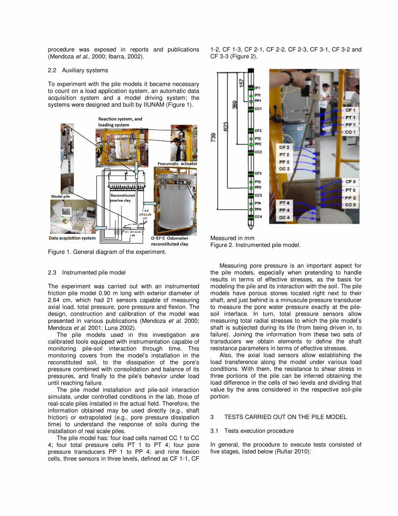
procedure was exposed in reports and publications (Mendoza et al., 2000; Ibarra, 2002). 2.2 Auxiliary systems To experiment with the pile models it became necessary to count on a load application system, an automatic data acquisition system and a model driving system; the systems were designed and built by IIUNAM (Figure 1).

Figure 1. General diagram of the experiment.

2.3 Instrumented pile model The experiment was carried out with an instrumented friction pile model 0.90 m long with exterior diameter of 2.64 cm, which had 21 sensors capable of measuring axial load, total pressure, pore pressure and flexion. The design, construction and calibration of the model was presented in various publications (Mendoza et al. 2000; Mendoza et al. 2001; Luna 2002).

The pile models used in this investigation are calibrated tools equipped with instrumentation capable of monitoring pile-soil interaction through time. This monitoring covers from the model’s installation in the reconstituted soil, to the dissipation of the pore’s pressure combined with consolidation and balance of its pressures, and finally to the pile’s behavior under load until reaching failure.

The pile model installation and pile-soil interaction simulate, under controlled conditions in the lab, those of real-scale piles installed in the actual field. Therefore, the information obtained may be used directly (e.g., shaft friction) or extrapolated (e.g., pore pressure dissipation time) to understand the response of soils during the installation of real scale piles.

The pile model has: four load cells named CC 1 to CC 4; four total pressure cells PT 1 to PT 4; four pore pressure transducers PP 1 to PP 4; and nine flexion cells, three sensors in three levels, defined as CF 1-1, CF

1-2, CF 1-3, CF 2-1, CF 2-2, CF 2-3, CF 3-1, CF 3-2 and CF 3-3 (Figure 2).

Measured in mm Figure 2. Instrumented pile model.

Measuring pore pressure is an important aspect for the pile models, especially when pretending to handle results in terms of effective stresses, as the basis for modeling the pile and its interaction with the soil. The pile models have porous stones located right next to their shaft, and just behind is a minuscule pressure transducer to measure the pore water pressure exactly at the pile-soil interface. In turn, total pressure sensors allow measuring total radial stresses to which the pile model’s shaft is subjected during its life (from being driven in, to failure). Joining the information from these two sets of transducers we obtain elements to define the shaft resistance parameters in terms of effective stresses.

Also, the axial load sensors allow establishing the load transference along the model under various load conditions. With them, the resistance to shear stress in three portions of the pile can be inferred obtaining the load difference in the cells of two levels and dividing that value by the area considered in the respective soil-pile portion. 3 TESTS CARRIED OUT ON THE PILE MODEL 3.1 Tests execution procedure In general, the procedure to execute tests consisted of five stages, listed below (Rufiar 2010):

Drive in:

• Alignment of the reinforced cap, the acrylic head and the steel plates in such a way that they allow the pile to pass through to do the test.

• Application of pressure outside the soil by means of the high pressure hydraulic jack and the help of four steel plates; the pressure applied to the soil sample was 73.5 kPa for the series named A and 147 kPa for the series named B. External pressure equal to 73.5 kPa was applied by means of a rigid element acting on the surface of the reconstituted clayey sample.

• Installation of the guiding frame and drive-in system on the oedometer.

• Connection of all the sensors of the pile model to the data acquisition system.

• Model pile driving by impacts, monitoring all sensors at this stage.

Post-drive-in:

• Monitoring of sensors placed in the pile, even after concluding the drive-in and almost for 24 hours.

• Installation of the reaction frame in the oedometer.

• Installation of the pneumatic actuator and LVTD displacement transducer.

• Verification of possible leaks in the pressurized-air line.

Test:

• Command programming for execution through the load application system.

• Monitoring in real time and data acquisition.

• Executing the test on the model pile with displacement control.

Total extraction of the pile model:

• Controlled displacement tests making use of the load application system.

• Total extraction using scaffolding and spindle. Hole filling:

• Preparation of a clayey mixture to fill the hole left by the extraction of the pile model from the oedometer soil.

• Injection of the mixture by means of a grease gun and hose.

The test program under monotonically increasing axial load was done considering the following factors:

Study the effect of the loading rate; for this, tests were made with monotonically increasing load varying the time to failure.

Study the effect of the various stress states on the soil’s mass where the piles were driven in, regarding the load-displacement relationship for the pile model. For this, two series of tests were programmed with different external applied pressures on the oedometer’s surface, in such a way that this clay was tested with two different conditions, one overconsolidated (OCR=2) and another normally consolidated (OCR=1). Thus, with the referred external pressures, existing stress conditions at two different depths were reproduced in the prototype.

Table 1. A-Series load tests (OCR = 1).

Test Characteristics

Displ. vel. Loading time

A-1 Compression 0.1 mm/min 11.13 min

Strain 0.1 mm/min 7.75 min

A-2 Compression 0.033 mm/min 46.63 min

Strain 0.033 mm/min 40.83 min

A-3 Compression 0.007 mm/min 119 min

Strain 0.007 mm/min 113 min

A-4 Compression 0.002 mm/min 717 min

Strain 0.002 mm/min 630 min

Table 2. B-Series load tests (OCR = 2).

Test Characteristics

Displ. Vel. Loading time

B-1 Compression 60 mm/min -

Strain 30 mm/min -

B-2 Strain 60 mm/min -

Compression 30 mm/min -

B-3 Compression 0.008 mm/min 121.03 min

Strain 0.008 mm/min 120.50 min

B-4 Compression 0.004 mm/min 840.01 min

Strain 0.004 mm/min 761.05 min

B-1a Compression 60 mm/min 0.043 min

Strain 30 mm/min 0.05 min

3.2 Sensor recording For each test a record was made of the number of necessary blows to drive in sections of 10 cm of the pile, up to its driving maximum length close to 70 cm.

It is important to indicate that the drive-in of the pile model in the test named B-1, under 147 kPa of external pressure, required many more blows to drive in 10 cm, than those necessary to drive in that same length with external pressure of 73.5 kPa. Considering this experience, and in view of the possibility of damaging the sensors, it was decided to drive in the rest of the tests of the B series without external pressure.

The graphic results of the number of blows are grouped on a band that shows more dispersion after the 20 cm drive-in; nonetheless, it can be said that in general the drive-in of the A series showed similar behaviour in all the tests, but the larger dispersion existent in the B series tests stands out. This could be due to the different drive-in maneuver times employed for one and the other series, which significantly affect resistance to the drive-in.

On the other hand, it is clear that there are some differences between the drive-in graphics for each test; in effect, test A1 required the least number of blows from the drive-in, whereas tests A2 and A3 required a similar number of blows. This could be due to the different drive-in maneuver times employed for one and the other test;

in effect, during test A3, for instance, there was a slight setback after the 10 cm drive-in, requiring a maneuver that took about 30 minutes. Upon continuing the drive-in, a notably larger number of blows (38) was required to drive in the next 10 cm than in the other two tests (16 and 25).

During the entire drive-in process for the A series tests, the reconstituted soil was subjected to external pressure, as explained before, so during this process the pile had to overcome the resistance offered by the soil. Therefore, as the pile was being driven in, the load cells already in contact with the soil recorded compression loads, and as time passed, these loads dissipated. Figure 3 shows the record of the four cells placed in the pile model (the minus sign indicates compression loads and the plus sign tension loads). We point out again that most of the tests of the B series were done without external pressure; pore pressure increases in the respective sensors were notably less than in those recorded for the A series. We have only included the results of the A series tests.

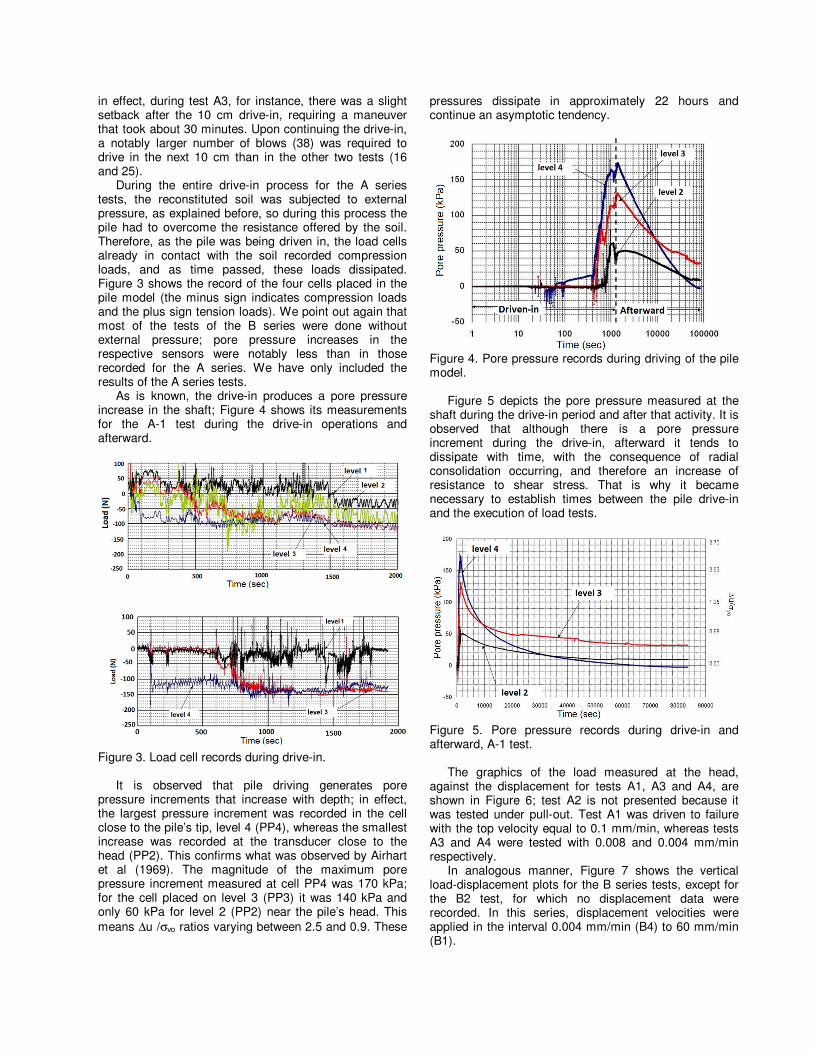
As is known, the drive-in produces a pore pressure increase in the shaft; Figure 4 shows its measurements for the A-1 test during the drive-in operations and afterward.

Figure 3. Load cell records during drive-in.

It is observed that pile driving generates pore

pressure increments that increase with depth; in effect, the largest pressure increment was recorded in the cell close to the pile’s tip, level 4 (PP4), whereas the smallest increase was recorded at the transducer close to the head (PP2). This confirms what was observed by Airhart et al (1969). The magnitude of the maximum pore pressure increment measured at cell PP4 was 170 kPa; for the cell placed on level 3 (PP3) it was 140 kPa and only 60 kPa for level 2 (PP2) near the pile’s head. This

means ∆u /σvo ratios varying between 2.5 and 0.9. These

pressures dissipate in approximately 22 hours and continue an asymptotic tendency.

Figure 4. Pore pressure records during driving of the pile model.

Figure 5 depicts the pore pressure measured at the

shaft during the drive-in period and after that activity. It is observed that although there is a pore pressure increment during the drive-in, afterward it tends to dissipate with time, with the consequence of radial consolidation occurring, and therefore an increase of resistance to shear stress. That is why it became necessary to establish times between the pile drive-in and the execution of load tests.

Figure 5. Pore pressure records during drive-in and afterward, A-1 test.

The graphics of the load measured at the head,

against the displacement for tests A1, A3 and A4, are shown in Figure 6; test A2 is not presented because it was tested under pull-out. Test A1 was driven to failure with the top velocity equal to 0.1 mm/min, whereas tests A3 and A4 were tested with 0.008 and 0.004 mm/min respectively.

In analogous manner, Figure 7 shows the vertical load-displacement plots for the B series tests, except for the B2 test, for which no displacement data were recorded. In this series, displacement velocities were applied in the interval 0.004 mm/min (B4) to 60 mm/min (B1).

Figure 8 shows the variation of the ultimate loads obtained considering the displacement velocity of the static load for both test series.

This figure shows that the more the load application velocity, the more the resistance. It also shows that the load capacity depends directly on the over-consolidation ratio; the more the confinement pressure, the more the load capacity.

Figure 6. Load-displacement curves, A series tests.

Figure 7. Load-displacement curves, B series tests.

Figure 8. Summary of load capacities for both series.

4 COMPARISON OF EXPERIMENTAL RESULTS AND VARIOUS METHODS

The practical design of friction piles faces a complex problem, for which frequently over-simplified and empirical or frankly heuristic solutions are chosen, that avoid important conditioning factors. Possibly the most relevant aspect of these refers to the pile’s installation process in the subsoil, because it usually entails significant changes in the states of stress and in the deformation field around the piles. This determines their reaction in terms of load and of the movements they experiment (Mendoza 2004).

Regarding the pile drive-in effects in clay, De Mello (1969) recognizes the following four large categories:

• Remolding or partial alteration of the subsoil structure next to the pile

• Alteration of the soil’s states of stress in the pile’s vicinity

• Pore pressure increase by drive-in and its dissipation around the pile

• Aging phenomenon Therefore, the pile installation method unquestionably

influences the soil-pile system’s load-deformation behavior, due to the changes from the soil’s initial state.

Then, the behaviour of the piles is influenced by the installation procedure, as well as by the changes experimented through time by the soil surrounding them. Therefore, the behaviour’s forecast must take into account in a realistic and practical manner the various situations and phenomena that occur from the drive-in, and then those derived from the application of sustained and transitory dynamic loads. The complete simulation of the displacing pile problem must then involve:

i) The installation process itself, which provokes soil changes, mainly radial from the pile’s shaft, with great distortions and remolding; the overcoming of the shear stress and the generation of high pore pressure increases.

ii) The occurrence of reconsolidation and adjustment of the effective stresses around the pile, as result of pore pressure dissipation.

iii) The process of sustained load incremental application until eventually reaching fluency conditions of the soil in contact with the pile.

vo

uc

σψ =

iv) The possible load capacity degradation due to the soil shear resistance decreasing because the dynamic actions and the posterior thixotropic processes, that determine the recovery of its resistance and consequently of the load capacity.

Nonetheless, within practical engineering drastic simplifications are adopted, which in the best of cases offer partial solutions to the situations described. Thus, the procedure initially proposed to estimate the mobilized resistance along the shaft of the friction piles was through the original and undrained shear strength of the soil where the piles are driven in.

For piles installed in clay, the Alpha method, used traditionally, and for many years practically the only one,

has been to define an adherence factor α as the ratio between adherence and undrained shear strength cu like this:

[1]

The results of these investigations have been presented as sets of empirical points, notoriously dispersed, of

values of α in function of the undrained shear strength of the soil. The authors of those works have proposed interpretations of this information for design, such as

value intervals for α, average curves for pile types or general average curves (Figure 9). From this adherence

factor α, resistance by lateral friction is calculated.

Figure 9. Adherence factor, various authors (after, McClelland, 1974).

It is a proven fact, with measurements made in a

case history of a foundation in Mexico City (Mendoza 2004), that the adherence-friction resistance at pile shafts is a fraction of the undrained shear strength; we

were able to verify that the quotient α acquires a value of 0.74. Nonetheless, this value refers to the clayey soil of Mexico City and not to marine clays, even if both are of soft consistency.

Tomlinson (1970) found that the ca/cu ratio may be markedly influenced by soil stratification, and suggests the factors shown in Table 3.

In the last 15 years improvements to the original proposal have been introduced, with which variables

such as pile length, overconsolidation ratio, and resistance ratio have been taken into account explicitly.

[2]

Table 3. Adherence factors for pile driving in stratified soils.

Case Soil conditions Penetration ratio

α

I Sands or sandy soils overlying stiff cohesive soils

< 20 1.25

<20

II Soft clays or silts overlying stiff cohesive soils

< 20 (>8) 0.40

> 20 0.70

III Stiff cohesive soils without overlying strata

< 20 (>8) 0.40

> 20

After Tomlinson (1970)

Penetration ratio =Depth of penetration in stiff clay

Pile diameter

Note 1: Adherence factors not applicable to H piles Note 2: Shaft adherence-friction in overburden soil for case I and II must be calculated separately. The American Petroleum Institute (API), in its design

code Recommended Practice 2A-WSD (RP 2A-WSD 2000), stipulates that for tubular piles installed in cohesive soils, shaft friction along the pile may be assessed by:

ucf α=

[3]

uc Undrained shear strength

α Adherence factor (dimensionless)

Recommending a value α close to the unit for clays in the Gulf of Mexico; nonetheless, the same code proposes

that the α ratio be valued at any depth as:

5.05.0

−= ψα for 0.1≤ψ [3a]

25.05.0

−= ψα for 0.1>ψ [3b]

On the other hand, it is a well established and proven

fact that failure in the shaft of a pile is governed by the Coulomb law of resistance in terms of effective stresses. Analyses of this type are known as Beta Methods. As result of remolding when installing a pile, the soil has no effective cohesion; this approach was adopted by Zeevaert (1959) and Eide and co-authors (1961) and has been widely documented by Burland (1973).

In the β-method proposed by Burland (1973), the pile shaft’s average friction can be determined in function of the parameters for effective stresses of the cohesive material in remolded state. Thus, for a given depth

vof βσ= [4]

here β is assessed as: K tanδ

K Lateral earth pressure coefficient

u

a

c

cα =

δ Drained friction angle between clay and pile

In its definition, β is related to the basic parameters

for effective stresses K and δ . In the case of piles in

normally consolidated clays, failure supposedly occurs in the thin zone of the pile shaft’s neighboring remolded

soil, so that dφδ = , where dφ is the remolded soil’s

drained friction angle. For a driven-in pile it could be

expected that K is larger than 0

K (lateral earth

pressure coefficient at rest) so that when taking 0

KK =

an inferior limit is adopted. For normally consolidated

clays, it is known that dsenK φ−= 10

. If these values

are replaced in the expression for β we obtain

( ) dsen φφβ tan1d

−= [5]

When considering in this expression values for dφ

in the interval from 20° to 30°, β varies between 0.24 and 0.29. This implies that in normally consolidated soft clays

β is not very sensitive to the internal friction angle. In

effect, average values for β from other expressions proposed by Burland (1973), Kerisel (1976) and Zeevaert (1973) fall within an interval from 0.25 to 0.35, Figure 10.

Determination of average values for β from load tests requires that these must be done after an adequate time after the installation, to guarantee resistance recovery.

Figure 10. β term, according to three different solutions (Mendoza 2004).

According to Meyerhof (1976), in the case of over-

consolidated clays (OCR>1) the following expression can

be used to calculate0

K :

( ) OCRK dφsin10

−= [6]

Where OCR is the overconsolidation ratio. Once the tests were concluded, we proceeded to

obtain representative undisturbed samples of the soil contained in oedometer O-97-5, with the purpose of carrying out fast and consolidated undrained triaxial

tests, to determine their mechanical properties (resistance to shear stress and internal friction angle, both in terms of total and effective stresses).

From the CU triaxial tests carried out on the reconstituted soil from O-97-5 oedometer, we obtained resistance parameters, measuring pore pressure at the failure stage.

To evaluate load capacity using different criteria both in terms of total and effective stresses, we employed the resistance parameters reported by the CU triaxial tests executed on the reconstituted soil.

Table 4 summarizes shaft load capacity obtained when using some of the methods described above; the shaft load capacity measured in test A-1 has been included.

We did the modeling of test A-1 (monotonically increasing axial load applied with displacement velocity of 0.1mm/min) using for it the numerical finite element method FEM, for which the grid composed by 5,795 nodes was built, and 661 triangular elements of 15 nodes. The code provides a fourth order interpolation for displacements and the numerical integration implies 12 Gauss points (points to evaluate stresses).

Due to the axi-symmetrical condition of the tests under study, only half pile and half the oedometer were modeled. Of course, the zone near the pile was discretized with more density of elements. Also, interface elements were placed between the pile’s shaft and the surrounding marine clay. An adherence-friction factor equivalent to 0.8 times the undrained shear strength of the soil was associated to the interface. A theoretical result closer to what was measured (Table 4) was obtained with an alpha value smaller than the one adopted. Table 4. Measured and theoretical shaft resistance

Method Theoretical shaft

resistance

Measured shaft resistance

α method α (Adim) Qfu (N) Qmeasured (N)

API (ec. 2, 3a and 3b)

(0.98 - 0.56) 1712 960

Tomlinson (ec 1 and Fig. 9)

(1.00 - 0.61) 1953 960

Kerisel (ec 4 and Fig. 9)

(0.98 - 0.65) 1905 960

β method β (Adim)

Burland (ec. 4) 0.26 1270 960

Kerisel (Fig. 10) 0.29 1422 960

Meyerhof (ec 6) 0.28 1348 960

The interface is the modeling of the interaction

between the pile and the soil, supposing that the contact surface is neither perfectly smooth nor perfectly rough. The contact’s degree of roughness is modeled choosing an adequate value for the reduction factor of the interface resistance. This factor relates the interface resistance

(pile friction and adherence) with the shear strength of the soil.

External pressure equal to 73.5 kPa was applied by means of a rigid cap acting on the surface of the clayey soil.

The marine soil was modeled following the Mohr-Coulomb resistance law with undrained behavior.

5 CONCLUSIONS As made evident by Table 4, the best approximation to the shaft load capacity in terms of total stresses

(α Method), is calculated using the criterion proposed by the API; then the criterion by Kerisel and last by Tomlinson, In general all these methods overestimate what was measured in the tests.

Similarly, Table 4 also shows that for the shaft load

capacity in terms of effective stresses (β Method), the best approximation is the one reported when using the finite elements technique (PLAXIS), because it overestimates what was measured by 25%. In general,

the β method in terms of effective stress defines closer

values to the measured capacity than the α method. During the tests made to the pile model, we

monitored continuously the load cells placed at different levels; thus we were able to obtain a lateral friction graphic. From that graphic, and previously knowing the

undrained shear strength, we determined an α value equal to 0.83.

Also, we monitored total stresses and pore pressure during those events, so we have the effective stresses acting on the pile’s shaft. At the time of failure, the shear stress measured was 25 kPa, and the effective vertical

stress was 78 kPa, thus obtaining a value for the term β equal to 0.32.

On the other hand, if it is known that the internal friction angle in terms of effective stresses is 23 degrees, according to the CU triaxial test measuring pore water pressure, and applying the equation (eq. 5) proposed by

Burland in 1973, a value for β can be obtained that is equal to 0.26; this value falls within the range proposed by that same author (0.24 to 0.29).

The average value for β measured during the A1 test was 0.32. The estimation calculated using the criterion proposed by Burland is 80% of what was measured. REFERENCES Airhart T.P., Coyle H.M., Hirsch T.J., y Buchananr S.J.

1969. Pile Soil System Response in a Cohesive Soil, Performance of Deep Foundations, ASTM, STP 444, ASTM, pp. 264-294

API, American Petroleum Institute 2000. Recommended Practice for Planning, Designing and Constructing Fixed Offshore Platforms –Working Stress Design, RP-2A-WSD, Washington, D.C. USA.

Burland, J. B. 1973. Shaft Friction of Piles in Clay –A Simple Fundamental Approach, Ground Engineering, Vol. 6(3), 30-42.

De Mello, V. F. B. 1969. Foundations of Buildings on Clay, State of the Art Report: 49-136. Proc. 7th ICSMFE, Mexico D.F, Vol. I, 1-86.

Eide, O., Hutchinson, J. N. and Landva, A. 1961. Short and Long-term Test Loading of a Friction Pile in Clay, Proc. 5th ICSMFE, Vol. 2, paper 38/8.

Ibarra, E. 2002. Reconstitution of a marine clayey soil in an oedometer for pile models testing [In Spanish], Master Thesis, DEP-FI, UNAM, Mexico D. F.

Kerisel, J. 1976. Contribución, Tercera Conferencia Nabor Carrillo, SMMS, Guanajuato, p 111.

Luna, O. J. 2002. Design, construction and operation of friction pile models under static and cyclic axial loads [In Spanish], Master Thesis, DEP-FI, UNAM, Mexico D. F.

Mendoza, M. J., Ibarra, E., Sánchez, J., Luna, O. J., y Orozco, M. 2000. Geotechnical characteristics of reconstituted clayey soils as alternative to the natural ones: Two uses [In Spanish], Memorias de la XX Reunión Nacional de Mecánica de Suelos, SMMS, Oaxaca, Mexico.

Mendoza, M. J., Luna, O. J., Ibarra, E., Romo, M. P., Barrera, P. and Olivares, A. 2001. Small-scale Models of Friction Piles in a Soft Marine Clay, Proc. 15th ICSMFE, Istanbul-Turkey, Vol. 2, 1307-1310.

Mendoza, M. J., Ibarra, E., Rufiar, M., Hinojosa J., Barrera P., Cruz D. 2004. Final Report: Response of the jacket foundation for an offshore plataform under cyclic and dynamic loads at Sonda de Campeche [In Spanish], Reporte para el Instituto Mexicano del Petróleo, Instituto de Ingeniería, UNAM.

Mendoza, M. J. 2004. Behavior of a friction piled foundation in Mexico City, under static and seismic loading [In Spanish], Doctoral Thesis, DEPFI, UNAM, Mexico, D.F.

Meyerhof G. G. 1976. Bearing Capacity and Settlement of Pile Foundations, ASCE, Journal of the Soil Mechanics and Foundations Division, Vol. 102., No. GT3, 195-228.

Pemex 2000. Design and evaluation for offshore plataforms at Sonda de Campeche [In Spanish], NRF-003-PEMEX-2000 Comité de Normalización de Petróleos Mexicanos y Organismos Subsidiarios, Mexico D.F.

Tomlinson, M. J. 1970. Some Effects of Pile Driving on Skin Friction, Conf. on Beh. of Piles, Inst. Civ. Engrs. London, pp 59-66.

Rufiar, M. 2010. Behavior of instrumented model piles under static axial loading in marine clayey soils [In Spanish], Master Thesis, SEPI, ESIA-IPN, Mexico, D.F.

Zeevaert, L. 1959. Reduction of Point-Bearing Capacity of Piles because of Negative Friction, Proc. First Panamerican Conf. on Soil Mech. and Found. Eng., Vol 3, Mexico, D.F., 1145-1152.

Zeevaert, L. 1973. Foundation Engineering for Difficult Subsoil Conditions, Van Nostrand Reinhold, New York.