Backwardation, Contango and Returns to Investors inCommodity Futures Markets

James Vercammen

University of British Columbia*

June, 2021

ABSTRACT

This paper proposes an alternative theory which connects the slope of the futures market for-

ward curve and expected returns for commodity-linked investors. The standard explanation for

why returns tend to be positive when the forward curve slopes down (i.e., backwardation) and

negative when the forward curve slopes up (i.e. contango) focuses on changes in the embed-

ded risk premium. The alternative proposed in this paper for the specific case of the U.S. corn

market is that USDA long-range demand forecasts exhibit slow-moving mean reversion which

is not accounted for by traders. Corn supply and demand forecasts from the USDA WASDE

reports are used to estimate intra-seasonal autoregressive forecasting equations. A calibrated

competitive storage model which incorporates these equations is used to establish a connection

between investor returns and market backwardation and contango. The annualized gain when

the investment is made with a positive roll yield (market backwardation) is about 4 percent, and

the annualized loss when the investment is made with a negative roll yield (market contango)

is also about 4 percent. This paper is unique it that it both identifies the source of the pricing

inefficiency and traces through its specific impact on traders.

Key words: commodity markets, investor returns, backwardation, contango, roll yield

JEL codes: G11, G13, Q11, Q14

*James Vercammen has a joint appointment with the Food and Resource Economics group and The SauderSchool of Business at the University of British Columbia. He can be contacted by mail at 2357 Main Mall, Van-couver, British Columbia, V6T 1Z4, by phone at (604) 822-5667, or by e-mail at james.vercammen@ubc.ca.

Backwardation, Contango and Returns to Investors in Commodity Futures

Markets

Running Head: Backwardation and Contango in Commodity Futures Markets

1 Introduction

The information content of forward curves in commodity futures markets is of considerable

interest to academics and trading professionals. Figure 1 shows the 8-contract forward curve

for Chicago Mercantile Exchange (CME) corn on two separate dates: July 2, 2020 and June

2, 2021. The July, 2020 forward curve is upward sloping and thus reflects a state of market

contango (also called a carry formation). The June, 2021 forward curve is downward sloping

(mostly) and thus reflects a state of market backwardation.1 The CME [2017] notes that in a

contango market there is over supply and/or low demand, and in a backwardated market there

is under supply and/or high demand. The CME also notes that inventories typically build when

a market is in contango and are depleted when a market is in backwardation. With reference

to Figure 1, the CME explanations shed light on the market contango in the early days of the

COVID-19 pandemic (i.e., July, 2020) and on the market backwardation in the recovery phase

of the pandemic (i.e., June, 2021).

This paper contributes to the literature which links the slope status of the forward curve

(i.e., backwardation versus contango) to the returns for investors who hold commodity-linked

investments such as commodity index funds, exchange traded funds (ETFs) and exchange traded

notes (ETNs).2 Although the popularity of these funds has decreased somewhat from a peak of

approximately $450 billion in 2012, they are still widely held by both retail and institutional

investors [Irwin et al., 2020]. Commodity-linked investments track a commodity index which

1In agricultural economics authors such as Carter [2012] uses "intertemporal pricing pattern" rather than "for-

ward curve" to describe the schedules in Figure 1. In the general finance literature, "forward curve" and "term

structure" are generally used to describe these schedules.2In the spring of 2021, the Invesco DB Agriculture Fund had assets of roughly $1 billion and the Teucrium

Corn Fund had assets of roughly $200 million.

1

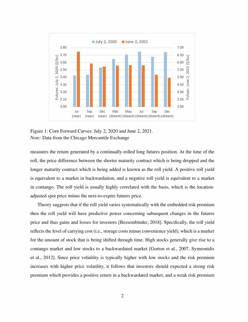
Figure 1: Corn Forward Curves: July 2, 2020 and June 2, 2021.Note: Data from the Chicago Mercantile Exchange

measures the return generated by a continually-rolled long futures position. At the time of the

roll, the price difference between the shorter maturity contract which is being dropped and the

longer maturity contract which is being added is known as the roll yield. A positive roll yield

is equivalent to a market in backwardation, and a negative roll yield is equivalent to a market

in contango. The roll yield is usually highly correlated with the basis, which is the location-

adjusted spot price minus the next-to-expire futures price.

Theory suggests that if the roll yield varies systematically with the embedded risk premium

then the roll yield will have predictive power concerning subsequent changes in the futures

price and thus gains and losses for investors [Bessembinder, 2018]. Specifically, the roll yield

reflects the level of carrying cost (i.e., storage costs minus convenience yield), which is a marker

for the amount of stock that is being shifted through time. High stocks generally give rise to a

contango market and low stocks to a backwardated market [Gorton et al., 2007, Symeonidis

et al., 2012]. Since price volatility is typically higher with low stocks and the risk premium

increases with higher price volatility, it follows that investors should expected a strong risk

premium which provides a positive return in a backwardated market, and a weak risk premium

2

which often provides a negative return in a contango market [Gorton et al., 2007, 2012, Dewally

et al., 2013, Bessembinder, 2018, Irwin et al., 2020]. It is important to keep in mind that the risk

premium which is associated with high price volatility is different than the hedging pressure risk

premium which long speculators collect from short hedgers in the Keynesian theory of normal

backwardation.

There is strong empirical evidence that the slope of the forward curve as measured by the

roll yield is correlated with the returns for commodity-linked investors. Using data from De-

cember 1992 to May 2004, Erb and Harvey [2006] calculated that eight commodities from a

group of 12 had both a negative average roll yield and a negative excess return. The remaining

four commodities were positive and positive. Similarly, using data from July 1959 to Decem-

ber 2004, Gorton and Rouwenhorst [2006] showed that the commodities with 50 percent of the

steepest (contango) forward curves had an excess return of -5.17 percent whereas the remain-

ing less steep (backwardation) forward curves had an excess return of 4.8 percent. Using data

between 1959 and 2014, Bhardwaj et al. [2015] showed that the percentage of commodities in

backwardation was positively associated with the subsequent month’s commodity index return.

More recently, Irwin et al. [2020] demonstrated a strong connection between roll yield and re-

turn when using cross commodity data, and a much weaker connection (largely due to high

price volatility) when using time series data.

It is puzzling that despite the strong theoretical and empirical connection between roll yield

and returns there is very little empirical evidence that the risk premium in of itself is a determi-

nant of investor returns. For example, Irwin et al. [2020] and the papers cited within conclude

that the unconditional return to holding futures tends to average to zero, and the returns for the

majority of the commodities are negative. This lack of consistency across these two empirical

literatures suggests that an explanation other than risk premium may be driving the relatively

strong connection between roll yield and investor returns.

In this paper, inefficient price forecasts which are not accounted for by traders provides an

alternative explanation. In the specific case of corn futures, this paper shows that non-anticipated

mean reversion in USDA forecasts of net market demand creates a link between roll yield and

market returns. This result is potentially important because monthly USDA global supply and

3

demand forecasts are an important source of information in the market for U.S. corn and other

agricultural commodities [Fortenbery and Sumner, 1993]. Mean reversion in the net market de-

mand forecast implies that the future price is expected to decrease over time when the initial

forecast is for strong future demand and the market is initially pulled into contango. Conversely,

the future price is expected to increase over time when the initial forecast is for weak future de-

mand and the market is initially pulled into backwardation. Similar to the previously cited liter-

ature, unconditional mean returns for commodity-linked investors are shown to approximately

equal zero whereas the conditional mean return is are positive if the investment is made in a

backwardated market and negative if the investment is made in a contango market.

These results are established using theory and simulation from a relatively simple com-

petitive storage model which has been calibrated to the U.S. corn market. The corn market is

used because it is the largest U.S. crop by production volume, and it is dominant in agricultural

futures trading.3 Central to the analysis is the strong econometric evidence that USDA World

Agricultural Supply and Demand Estimates (WASDE) forecasts of longer-term net market de-

mand are mean reverting with serially correlated errors rather than behaving as an information-

efficient random walk. Nordhaus [1987] notes that a forecast is weakly efficient if the cur-

rent forecast errors are independent of past forecast errors, and this condition is equivalent to

fixed-event forecasts following a random walk. Nordhaus cites several examples of inefficient

fixed-event forecasting and so it should not be surprising that the USDA forecasts are also not

informationally efficient. If the forecast mean reversion is anticipated by traders, similar to how

mean reversion in spot markets are assumed to be anticipated by traders [Bessembinder et al.,

1995], then futures prices will neither systematically increase or decrease over time, and in-

vestor returns will average to zero. If instead traders fail to anticipate this mean reversion then

the aforementioned relationship between the status of the forward curve and investor returns

will emerge.

3According to the Chicago Mercantile Exchange (CME) website, on June 7, 2021 prior day open interest was

1,720,385 for corn and 4,919,523 for overall agriculture, which gives corn a 35.0 percent share in agricultural

futures trading.

4

The extent that traders account for mean reversion in USDA forecasts is in the domain of the

informational efficiency of futures markets. Bohl et al. [2020] provides a good overview of the

relevant literature and they find significant temporal and cross-sectional variation in market effi-

ciency in 19 commodity futures markets. Bohl et al. [2020] and Carter [2012] both conclude that

unequally informed traders are a major reason for pricing inefficiency. This conjecture is consis-

tent with the well-documented roll yield myth, which asserts that investing in a contango market

locks in a negative roll yield as a loss when an expiring contract is rolled into a new contract,

and opposite for the case of a backwardated market [Sanders and Irwin, 2012, Bessembinder,

2018, Irwin et al., 2020].4 More generally, there is considerable evidence that spot and futures

prices in commodity markets are not fully arbitraged in the way theory suggests [Buccola, 1989,

Beck, 1994, Kellard et al., 1999, McKenzie and Holt, 2002, Adjemian et al., 2013, Bosch and

Pradkhan, 2016]. Consequently, it is reasonable to assume that the mean reversion in the USDA

net demand forecasts is not fully accounted for in commodity price formation.

This paper’s competitive storage model, which is calibrated to the U.S. corn market, con-

sists of two consecutive crop years divided into eight quarters with harvest taking placing at

the beginning of each crop year (i.e., Q1 and Q5). Stocks are carried through time and the

merchant’s marginal carrying costs are just covered by expected price changes. The model is

closed by assuming that stocks are carried out of Q8 according to an exogenous "year 3" net

demand for starting stocks. Stochastic prices are obtained by randomly generating a forecast

for Q5 production at the beginning of Q2 through Q5, and randomly generating a forecast for

year 3 net demand at the beginning of Q2 through Q8. The pair of forecasts in Q2 result in a

particular slope for the Q2 forward curve, and it is this slope which defines the relevant roll

yield. With each new forecast the model is resolved to generate a revised set of prices. Unique

futures contracts exist for each quarter and their prices are equal to the expected spot prices at

the point of contract expiry. Investor profits are calculated as either the Q2 to Q8 stochastic price

4According to VanEck [2013] the 10-year S&P GSCI roll yield for corn to the end of 2012 was -12.06 percent,

which represents a moderately high average level of contango (the equivalent values for live hogs, cotton and

soybeans is -16.7, -2.20 and 1.01 percent, respectively). Van Eck Global warned investors about potentially large

loses when investing in a contango market.

5

difference for a Q8 futures contract ("buy-and-hold") or the Q2 to Q4 stochastic price difference

for a Q4 futures contract plus the Q4 to Q8 stochastic price difference for a Q8 futures contract

("buy-and-roll").

The main results concerning investor returns and the roll yield are established analytically

and are further illustrated through use of Monte Carlo simulation. One set of the 10,000 sim-

ulated model outcomes generates one Q2 measure of roll yield, a sequence of eight quarterly

spot prices, seven forward curves and two measures of investor profits. The 10,000 sets of sim-

ulated data are categorized according to positive Q2 roll yield (backwardation) and negative Q2

roll yield (contango), and subsequent investor profits are averaged within each category. Fixed

effects panel estimation allows within measures of price volatility, and autocorrelation to be

efficiently estimated with the 80,000 observations. Despite the simple structure of the compet-

itive storage model, the stochastic prices are shown to have realistic properties. The outcome

that the annualized conditional expected profit or loss for an investor is about 4.3 percent is also

realistic, and is consistent with other estimates such as Gorton and Rouwenhorst [2006].

The intuition for the main results is most easily explained when the supply forecast is fixed

at its mean level. In this case, if the USDA forecast for year 3 net demand increases from zero

to positive then additional stocks move forward through time, the market’s carrying cost rises,

the forward curve slopes up and the roll yield takes on a negative value. As the net demand

forecast gradually reverts towards its mean value of zero the volume of stocks carried forward

decreases and the expected roll yield becomes less negative. Initiating the investment when the

roll yield is more negative and terminating it when it is less negative results in an expected loss

for the investor. The intuition for the backwardated market outcome is the mirror image of that

described above.

A number of other unique results emerge from the analysis. First, similar price trends emerge

in the spot and futures markets, which is different than the standard analysis where a change

in the risk premium affects the futures price relative to the spot price. This means that even

though spot markets are arbitraged in the short run (i.e., carrying costs equal the expected price

increase) any merchant who carries the stock in the long run will experience the same loss or

gain as the investor in the futures market. Second, the structure of the futures roll affects the size

6

of the expected loss and gain. Less frequent rolls (e.g., rolling the contract every fourth month

rather than every second month) results in larger expected profits in a backwardated market and

larger expected losses in a contango market.5 Third, a trend in the futures prices may or may

not be equivalent to mean reversion in the futures price. For example, in a contango market the

futures price may start above its long run mean and then trend down toward it, or the futures

price may start below its long run mean and then continue to trend down. These results emerge

because USDA supply forecasts affect the position of the initial price but have no affect on how

the futures price trends over time.

In the next section a non-stochastic version of the competitive storage model is constructed

and solved to obtain spot and futures prices expressed as linear functions of the two forecast

variables. The assumptions and equations which describe the forecasting and information updat-

ing by market participants is then incorporated into the model. Section 3 is used to calibrate the

model to the U.S. corn market. The calibration includes demonstrating that the autoregressive

equations which govern the stochastic forecasts are consistent with a random walk specification

for the Q5 production forecasts and are consistent with mean reversion for the year 3 net de-

mand forecasts. Section 3 concludes by comparing the summary statistics from the 10,000 sets

of simulated prices with real-world outcomes in the corn market. The main results concerning

the relationship between the slope status of the forward curve (i.e., backwardation versus con-

tango) and expected profits for investors are presented in Section 4. Concluding comments are

provided in Section 5.

5In the Goldman Sachs Commodity Index corn futures are rolled over five times each year whereas crude oil

futures are rolled over monthly. The roll yield myth implies that more frequent rolling generates higher returns

in a backwardated market and higher losses in a contango market. This is opposite the results from this current

analysis.

7

2 Competitive Storage Pricing Model

The first subsection below describes the non-stochastic version of the competitive storage model.

The additional assumptions which are used to make the model stochastic are described in the

second subsection.

2.1 Non Stochastic Version of the Model

The single-location market operates for two years with each year subdivided into four quarters.

Harvest in year 1 occurs in Q1 at level H1 and harvest in year 2 occurs in Q5 at level H5.6

Let St denote stocks which are carried out of quarter t and into quarter t + 1. An important

variable is S8, which is a measure of the unconsumed stocks at the terminal date. Assume there

exists an exogenous (perfectly inelastic) year 3 demand for these Q8 stocks. This demand can

be broken down into normal-year "pipeline" stocks, S0, plus a deviation from normal demand,

D, which later in the analysis is made stochastic. At the beginning of Q1 normal-year pipeline

stocks, S0, combine with a normal-sized harvest, H1, to create a stockpile which is available for

consumption in year 1. In the empirical analysis S0 and H1 are assumed to represent long-term

average values.

Inverse demand in quarter t is given by Pt = a − bXt where Pt is the market price and Xt

is the level of consumption. The assumption that the demand schedule remains constant over

time implies that the seasonality in prices which is examined below is not the result of seasonal

shifts in demand. The merchants’ marginal cost of storing the commodity from one quarter to

the next consists of a physical storage cost and an opportunity cost of the capital which is tied

up in the inventory. The combined marginal cost of storage is given by the increasing function

kt = k0 + k1St.7 This specification ensures that the marginal storage cost is highest in the

6Q1 and Q5 correspond to October to December, Q2 and Q6 correspond to January to March, Q3 and Q7 corre-

spond to April to June, and Q4 and Q8 correspond to July to September. These dates were chosen to approximately

align with the U.S. corn harvest and with data availability.7The equilibrium price is shown to be a linear function of St and so the opportunity cost of capital, which is

proportional to the commodity’s price, is embedded in the k0 and k1 parameters.

8

fall quarter (i.e., Q1 and Q5) when stocks are at a maximum, and it gradually declines as the

marketing year progresses.

Merchants also receive a convenience yield from owning the stocks rather than having to

purchase stocks on short notice.8 Let ct = c0 − c1St denote the marginal convenience yield for

quarter t. This function decreases with higher stocks because of the diminished convenience

from owning stocks when stocks are plentiful in the market [Working, 1948, 1949]. Marginal

carrying cost is given by the difference between marginal storage cost and marginal carrying

cost; i.e., mt = kt − ct. As will be shown below, this net carrying cost cycles between positive

and negative values within the crop year.

According to the carrying charge theory of commodity pricing [Kaldor, 1939, Working,

1948, 1949, Brennan, 1958, Telser, 1958], competition between merchants ensures that the

compensation for supplying storage, Pt+1 − Pt, is equal to the marginal carrying cost, mt.

Substituting in the expressions for kt and ct allows the supply of storage equation (sometimes

referred to as the intertemporal law-of-one-price equation) to be written as Pt+1 − Pt = m0 +

m1St where m0 = k0 − c0 and m1 = k1 + c1.9

The equations which define the set of equilibrium prices, consumption and stocks can be

written as

Pt+1 − Pt = m0 +m1St (1)

Pt = a− bXt (2)

S1 = S0 +H1 −X1, S5 = S4 +H5 −X5, S8 = S0 +D,

St = St−1 −Xt for t = 2, 3, 4, 6, 7, 8(3)

8A standard explanation of convenience yield is that stocks on hand allow merchants to fill unexpected orders

and create unexpected sales opportunities at a lower transaction cost. Carter [2012] likens convenience yield to the

liquidity value of cash on hand versus cash allocated to a locked-in investment.9This version of the stochastic storage model is less general than the standard version [Williams and Wright,

1991, Deaton and Laroque, 1996, Routledge et al., 2000] because there is no allowance for a stock out (i.e., St = 0).

The absence of a potential corner solution ensures that the pricing model has a closed-form solution.

9

Equation (3) is the equation of motion, which ensures that ending stocks must equal beginning

stocks plus harvest minus consumption.

In the Appendix it is shown that the solution to equations (1) to (3) can be expressed as

linear functions of the H5 and D exogenous variables. Specifically, Pt = δt0 + δt1H5 + δt2D for

t = 1, 2, ..., 8 where δt0, δt1 and δt2 are time-dependent, recursive functions of the core parameters:

a, b, m0, m1, S0 and H1. In the next section the model is made stochastic by assuming that H5

and D take on random values, and the forecasts for these two variables are updated at the

beginning of each quarter.10

To conclude this section note that the model can be solved beginning in any of the eight

quarters. Suppose it is the beginning of Q3 and the value of the H5 variable is updated. The

solution for the remaining six quarters can be updated by resolving equations (1) to (3) for

t = 3, 4, ..., 8 with the new H5 value and with S3 = S∗2 where S∗

2 comes from the solution in

Q2.

2.2 Stochastic Version of the Model

After harvest is complete in Q1 there are two sources of future uncertainty. The first is the size

of the (year 2) Q5 harvest, H5, and the second is the net demand component, D, of the year

3 demand for beginning stocks. Let H denote the stochastic version of the H5 variable, for

t = 1, ..., 5 and let Ht denoted the quarter t forecasted value of H where H5 = H . Similarly,

let D denote the stochastic version of the D variable, and for t = 1, 2, ..., 8 let Dt denote the

quarter t forecasted value of D with D8 = D.

10The stochastic values for H5 and D should realistically depend on the set of prices expected for Q5 through

Q8. The simplifying assumption that these variables are exogenous is unlikely to be important for the general

interpretation of the results.

10

The linearity of the pricing model implies that the spot price which is expected in quarter

t + s and which is conditional on the quarter t forecasts, can be specified by substituting the

pair of forecasts into Pt = δt0 + δt1H5 + δt2D to obtain11

Et(Pt+s|Ht, Dt) = δt+s0 + δt+s1 Ht + δt+s2 Dt s = 0, 1, ..., 8− t (4)

Note that within equation (4) the actual level of Q5 production, H5, is substituted for the non-

existent Ht when t = 6, 7, 8. In quarter t + 1 when new forecasts become available, a new set

of expected spot prices can be generated using the same procedure. If the forecast updates are

generated by a defined stochastic process, then this process can be combined with equation (4)

to create a stochastic expected price sequence.

Assume that in quarter t there are 8 − t futures contracts which trade, one which expires

in quarter t + 1, one which expires in quarter t + 2, etc. Let F t+st denote the quarter t price of

a futures contract which expires in quarter t + s. Given the assumption of risk neutral traders

and unbiased price expectations, the futures price is equal to the spot price which is expected

when the contract expires. Using equation (4) an expression for F t+st conditioned on the current

forecast can be written as

F t+st (Ht, Dt) = δt+s0 + δt+s1 Ht + δt+s2 Dt s = 0, 1, ..., 8− t (5)

Equation (5) is the quarter t forward curve conditioned on the quarter t forecasts.

The next step is to describe more specifically how the two forecasts, Ht and Dt, are ran-

domly generated each quarter. It is useful to decompose Ht into the product of forecasted har-

vested acres and forecasted yield. Forecasted acres, At, and the log of forecasted yield, Yt are

both independently drawn from normal distributions. With these assumptions it follows that

Ht = Atexp(Yt). Forecasted net demand, Dt, is also drawn from a normal distribution.

The forecasts for Q1 are assumed to be fixed at their long term average values, which is A

for harvested acres, Y for yield, and 0 for year 3 net demand. The Q2 forecast for harvested

acres is drawn from a normal distribution with mean A and standard deviation σA. The log of

11The implicit assumption is thatEt(Ht+s) = Ht. This assumption would not hold if Ht systematically changed

over time and the change was anticipated by traders.

11

the Q2 forecast for yield is drawn from a normal distribution with mean Yln = ln(Y ) − 0.5σY

and standard deviation σY . There is no data available to estimate the standard deviation of the

Q2 forecast of year 3 net demand. As an alternative, the Q3 forecast for net demand is drawn

from a normal distribution with mean 0 and standard deviation σD. The difference between

the Q2 forecast and the Q3 forecast for net demand is assumed to be a normally distributed

random variable with mean zero and standard deviation σD4 (more details about this assumption

are provided below).

The various standard deviation measures in the previous paragraph are "between" measures

of forecast uncertainty because they represent forecasts across different crop year simulations

rather than forecasts within a particular crop year simulation. For the net demand forecast, σD

is set equal to the standard deviation of the Q3 demand forecasts across the 25 years in the

USDA forecasting data set. The situation is similar for acreage and yield except the time trend

is removed from the USDA data across years before estimating the standard deviation.

For Q3, Q4 and Q5, the forecasted values for acres and yield require within estimates rather

than between estimates. A simple and effective way to estimate intertemporal forecast linkages

within a crop year is through use of an autoregressive stochastic process with one lag (i.e., an

AR(1)). The AR(1) stochastic processes for the acres forecast and the log of yield forecast are

given by At = βAt +γAt At−1 +eAt and Yt = βYt +γYt Yt−1 +eYt , respectively. For Q4 through Q8

the forecasted values for net demand are also assumed to be generated with an AR(1) process:

Dt = βDt + γDt Dt−1 + eDt . The coefficients of these equations have a time index because they

will eventually be estimated with panel data and with intercept and slope fixed effects.

The specific procedure for using the estimated regression equations to generate forecasts for

Q3 and beyond is as follows. Let σYt , σAt and σDt denote the standard deviation of the regres-

sion residuals, eAt , eYt and eDt respectively. The simulated acreage forecast for Q3 is given by

A3 = βA3 + γA3 A2 plus a normally distributed error term with mean 0 and standard deviation σA3 .

The yield forecast for Q3 is given by exp(βY2 + γY2 Y2

)plus the exponential of a normally dis-

tributed error term with mean 0 and standard deviation σY3 . This method of generating forecasts

is used for all three forecast variables. The complete set of assumptions and equations which

govern forecasting are summarized in Table 1.

12

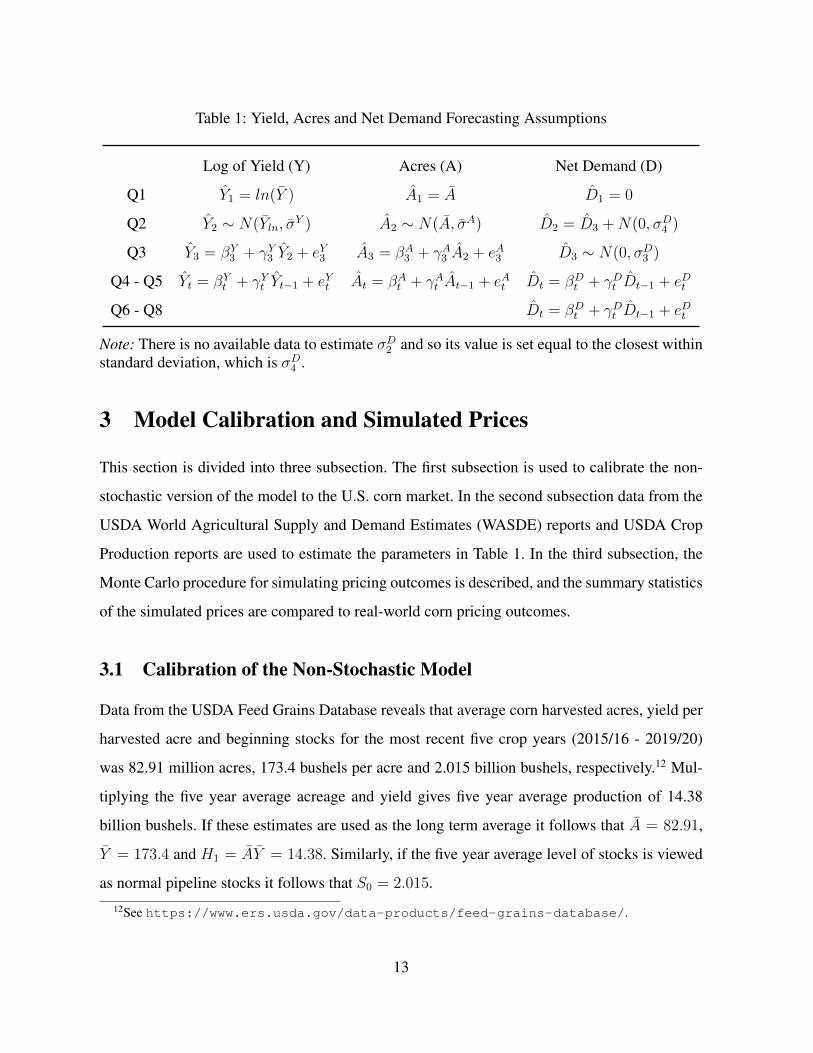
Table 1: Yield, Acres and Net Demand Forecasting Assumptions

Log of Yield (Y) Acres (A) Net Demand (D)

Q1 Y1 = ln(Y ) A1 = A D1 = 0

Q2 Y2 ∼ N(Yln, σY ) A2 ∼ N(A, σA) D2 = D3 +N(0, σD4 )

Q3 Y3 = βY3 + γY3 Y2 + eY3 A3 = βA3 + γA3 A2 + eA3 D3 ∼ N(0, σD3 )

Q4 - Q5 Yt = βYt + γYt Yt−1 + eYt At = βAt + γAt At−1 + eAt Dt = βDt + γDt Dt−1 + eDt

Q6 - Q8 Dt = βDt + γDt Dt−1 + eDt

Note: There is no available data to estimate σD2 and so its value is set equal to the closest withinstandard deviation, which is σD4 .

3 Model Calibration and Simulated Prices

This section is divided into three subsection. The first subsection is used to calibrate the non-

stochastic version of the model to the U.S. corn market. In the second subsection data from the

USDA World Agricultural Supply and Demand Estimates (WASDE) reports and USDA Crop

Production reports are used to estimate the parameters in Table 1. In the third subsection, the

Monte Carlo procedure for simulating pricing outcomes is described, and the summary statistics

of the simulated prices are compared to real-world corn pricing outcomes.

3.1 Calibration of the Non-Stochastic Model

Data from the USDA Feed Grains Database reveals that average corn harvested acres, yield per

harvested acre and beginning stocks for the most recent five crop years (2015/16 - 2019/20)

was 82.91 million acres, 173.4 bushels per acre and 2.015 billion bushels, respectively.12 Mul-

tiplying the five year average acreage and yield gives five year average production of 14.38

billion bushels. If these estimates are used as the long term average it follows that A = 82.91,

Y = 173.4 and H1 = AY = 14.38. Similarly, if the five year average level of stocks is viewed

as normal pipeline stocks it follows that S0 = 2.015.

12See https://www.ers.usda.gov/data-products/feed-grains-database/.

13

The two parameters from the demand equation are set to a = 16.21 and b = 3.5. These

parameters ensure that the average price across all eight quarters is $3.628/bu, which is very

close to the $3.648/bu average farm gate price for 2016 - 2020. Moreover, the demand elasticity,

which is calculated with the simulated $3.628/bu average quarterly price and the simulated

3.595 billion bushel average quarterly consumption, is equal to -0.288. This simulated elasticity

is reasonably close to the -0.2 corn demand elasticity estimate which was reported by Moschini

et al. [2017].

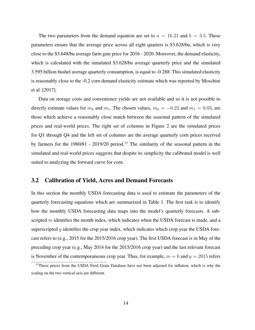
Data on storage costs and convenience yields are not available and so it is not possible to

directly estimate values for m0 and m1. The chosen values, m0 = −0.22 and m1 = 0.03, are

those which achieve a reasonably close match between the seasonal pattern of the simulated

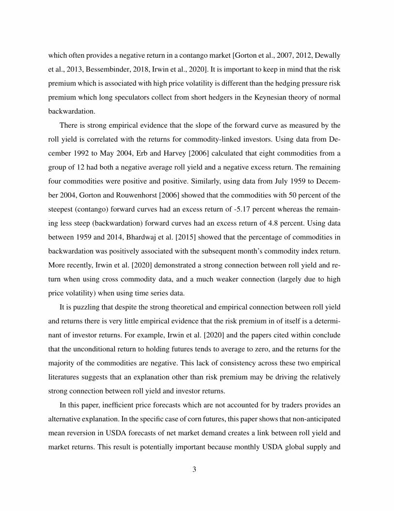
prices and real-world prices. The right set of columns in Figure 2 are the simulated prices

for Q1 through Q4 and the left set of columns are the average quarterly corn prices received

by farmers for the 1980/81 - 2019/20 period.13 The similarity of the seasonal pattern in the

simulated and real-world prices suggests that despite its simplicity the calibrated model is well

suited to analyzing the forward curve for corn.

3.2 Calibration of Yield, Acres and Demand Forecasts

In this section the monthly USDA forecasting data is used to estimate the parameters of the

quarterly forecasting equations which are summarized in Table 1. The first task is to identify

how the monthly USDA forecasting data maps into the model’s quarterly forecasts. A sub-

scripted m identifies the month index, which indicates when the USDA forecast is made, and a

superscripted y identifies the crop year index, which indicates which crop year the USDA fore-

cast refers to (e.g., 2015 for the 2015/2016 crop year). The first USDA forecast is in May of the

preceding crop year (e.g., May 2014 for the 2015/2016 crop year) and the last relevant forecast

is November of the contemporaneous crop year. Thus, for example, m = 6 and y = 2015 refers

13These prices from the USDA Feed Grain Database have not been adjusted for inflation, which is why the

scaling on the two vertical axis are different.

14

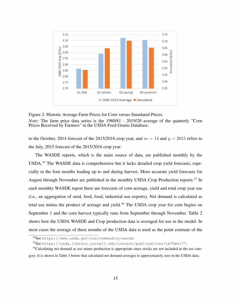
Figure 2: Historic Average Farm Prices for Corn versus Simulated Prices.Note: The farm price data series is the 1980/81 - 2019/20 average of the quarterly "CornPrices Received by Farmers" in the USDA Feed Grains Database.

to the October, 2014 forecast of the 2015/2016 crop year, and m = 14 and y = 2015 refers to

the July, 2015 forecast of the 2015/2016 crop year.

The WASDE reports, which is the main source of data, are published monthly by the

USDA.14 The WASDE data is comprehensive but it lacks detailed crop yield forecasts, espe-

cially in the four months leading up to and during harvest. More accurate yield forecasts for

August through November are published in the monthly USDA Crop Production reports.15 In

each monthly WASDE report there are forecasts of corn acreage, yield and total crop year use

(i.e., an aggregation of seed, feed, food, industrial use exports). Net demand is calculated as

total use minus the product of acreage and yield.16 The USDA crop year for corn begins on

September 1 and the corn harvest typically runs from September through November. Table 2

shows how the USDA WASDE and Crop production data is averaged for use in the model. In

most cases the average of three months of the USDA data is used as the point estimate of the

14See https://www.usda.gov/oce/commodity/wasde.15See https://usda.library.cornell.edu/concern/publications/tm70mv177.16Calculating net demand as use minus production is appropriate since stocks are not included in the use cate-

gory. It is shown in Table 3 below that calculated net demand averages to approximately zero in the USDA data.

15

quarterly forecast. If three months of data do not exist for a particular quarter then one month

of USDA data is used as the estimate of the quarterly forecast.

Table 2: Mapping of USDA Forecast Months to Model Forecast Quarters

Q2 Q3 Q4 Q5

Acres (9− 11)W (12− 14)W (15− 17)W 19W

Yield (9− 11)W (12− 14)W 16P 19P

Demand na 1W (3− 5)W (6− 8)W

Q6 Q7 Q8

Demand (9− 11)W (12− 14)W (15− 17)W

Note: (a) The numbers are the month index, beginning with 1 for May of the preceding crop yearand ending with 19 for November of the contemporaneous year; (b) The parenthesis indicate aquarterly average; (c) The "W" superscript indicates WASDE monthly data and "P" indicatesCrop Production monthly data.

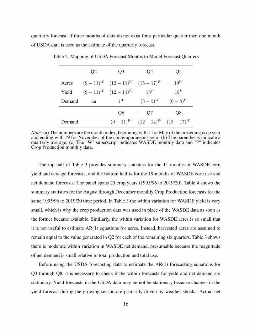
The top half of Table 3 provides summary statistics for the 11 months of WASDE corn

yield and acreage forecasts, and the bottom half is for the 19 months of WASDE corn use and

net demand forecasts. The panel spans 25 crop years (1995/96 to 2019/20). Table 4 shows the

summary statistics for the August through December monthly Crop Production forecasts for the

same 1995/96 to 2019/20 time period. In Table 3 the within variation for WASDE yield is very

small, which is why the crop production data was used in place of the WASDE data as soon as

the former became available. Similarly, the within variation for WASDE acres is so small that

it is not useful to estimate AR(1) equations for acres. Instead, harvested acres are assumed to

remain equal to the value generated in Q2 for each of the remaining six quarters. Table 3 shows

there is moderate within variation in WASDE net demand, presumable because the magnitude

of net demand is small relative to total production and total use.

Before using the USDA forecasting data to estimate the AR(1) forecasting equations for

Q3 through Q8, it is necessary to check if the within forecasts for yield and net demand are

stationary. Yield forecasts in the USDA data may be not be stationary because changes in the

yield forecast during the growing season are primarily driven by weather shocks. Actual net

16

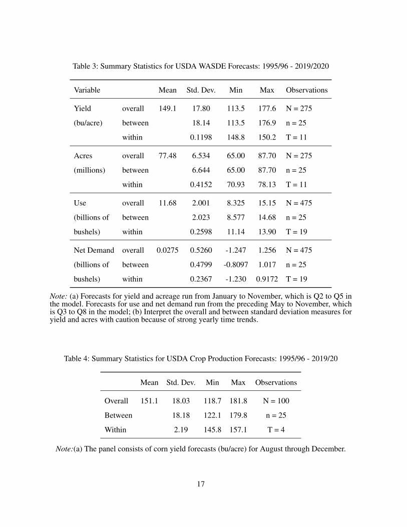
Table 3: Summary Statistics for USDA WASDE Forecasts: 1995/96 - 2019/2020

Variable Mean Std. Dev. Min Max Observations

Yield overall 149.1 17.80 113.5 177.6 N = 275

(bu/acre) between 18.14 113.5 176.9 n = 25

within 0.1198 148.8 150.2 T = 11

Acres overall 77.48 6.534 65.00 87.70 N = 275

(millions) between 6.644 65.00 87.70 n = 25

within 0.4152 70.93 78.13 T = 11

Use overall 11.68 2.001 8.325 15.15 N = 475

(billions of between 2.023 8.577 14.68 n = 25

bushels) within 0.2598 11.14 13.90 T = 19

Net Demand overall 0.0275 0.5260 -1.247 1.256 N = 475

(billions of between 0.4799 -0.8097 1.017 n = 25

bushels) within 0.2367 -1.230 0.9172 T = 19

Note: (a) Forecasts for yield and acreage run from January to November, which is Q2 to Q5 inthe model. Forecasts for use and net demand run from the preceding May to November, whichis Q3 to Q8 in the model; (b) Interpret the overall and between standard deviation measures foryield and acres with caution because of strong yearly time trends.

Table 4: Summary Statistics for USDA Crop Production Forecasts: 1995/96 - 2019/20

Mean Std. Dev. Min Max Observations

Overall 151.1 18.03 118.7 181.8 N = 100

Between 18.18 122.1 179.8 n = 25

Within 2.19 145.8 157.1 T = 4

Note:(a) The panel consists of corn yield forecasts (bu/acre) for August through December.

17

demand is expected to be mean reverting toward zero due to the standard forces of supply and

demand.17 However, the outcome that USDA net demand forecasts are also mean reverting was

unexpected because such an outcome is not informationally efficient.

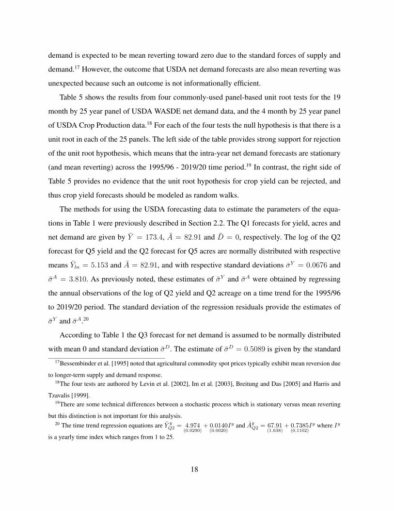
Table 5 shows the results from four commonly-used panel-based unit root tests for the 19

month by 25 year panel of USDA WASDE net demand data, and the 4 month by 25 year panel

of USDA Crop Production data.18 For each of the four tests the null hypothesis is that there is a

unit root in each of the 25 panels. The left side of the table provides strong support for rejection

of the unit root hypothesis, which means that the intra-year net demand forecasts are stationary

(and mean reverting) across the 1995/96 - 2019/20 time period.19 In contrast, the right side of

Table 5 provides no evidence that the unit root hypothesis for crop yield can be rejected, and

thus crop yield forecasts should be modeled as random walks.

The methods for using the USDA forecasting data to estimate the parameters of the equa-

tions in Table 1 were previously described in Section 2.2. The Q1 forecasts for yield, acres and

net demand are given by Y = 173.4, A = 82.91 and D = 0, respectively. The log of the Q2

forecast for Q5 yield and the Q2 forecast for Q5 acres are normally distributed with respective

means Yln = 5.153 and A = 82.91, and with respective standard deviations σY = 0.0676 and

σA = 3.810. As previously noted, these estimates of σY and σA were obtained by regressing

the annual observations of the log of Q2 yield and Q2 acreage on a time trend for the 1995/96

to 2019/20 period. The standard deviation of the regression residuals provide the estimates of

σY and σA.20

According to Table 1 the Q3 forecast for net demand is assumed to be normally distributed

with mean 0 and standard deviation σD. The estimate of σD = 0.5089 is given by the standard

17Bessembinder et al. [1995] noted that agricultural commodity spot prices typically exhibit mean reversion due

to longer-term supply and demand response.18The four tests are authored by Levin et al. [2002], Im et al. [2003], Breitung and Das [2005] and Harris and

Tzavalis [1999].19There are some technical differences between a stochastic process which is stationary versus mean reverting

but this distinction is not important for this analysis.20 The time trend regression equations are Y y

Q2 = 4.974(0.0290)

+ 0.0140(0.0020)

Iy and AyQ2 = 67.91

(1.638)+ 0.7385

(0.1102)Iy where Iy

is a yearly time index which ranges from 1 to 25.

18

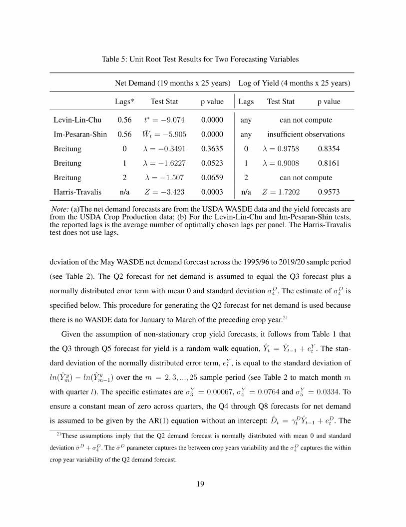
Table 5: Unit Root Test Results for Two Forecasting Variables

Net Demand (19 months x 25 years) Log of Yield (4 months x 25 years)

Lags* Test Stat p value Lags Test Stat p value

Levin-Lin-Chu 0.56 t∗ = −9.074 0.0000 any can not compute

Im-Pesaran-Shin 0.56 Wt = −5.905 0.0000 any insufficient observations

Breitung 0 λ = −0.3491 0.3635 0 λ = 0.9758 0.8354

Breitung 1 λ = −1.6227 0.0523 1 λ = 0.9008 0.8161

Breitung 2 λ = −1.507 0.0659 2 can not compute

Harris-Travalis n/a Z = −3.423 0.0003 n/a Z = 1.7202 0.9573

Note: (a)The net demand forecasts are from the USDA WASDE data and the yield forecasts arefrom the USDA Crop Production data; (b) For the Levin-Lin-Chu and Im-Pesaran-Shin tests,the reported lags is the average number of optimally chosen lags per panel. The Harris-Travalistest does not use lags.

deviation of the May WASDE net demand forecast across the 1995/96 to 2019/20 sample period

(see Table 2). The Q2 forecast for net demand is assumed to equal the Q3 forecast plus a

normally distributed error term with mean 0 and standard deviation σD4 . The estimate of σD4 is

specified below. This procedure for generating the Q2 forecast for net demand is used because

there is no WASDE data for January to March of the preceding crop year.21

Given the assumption of non-stationary crop yield forecasts, it follows from Table 1 that

the Q3 through Q5 forecast for yield is a random walk equation, Yt = Yt−1 + eYt . The stan-

dard deviation of the normally distributed error term, eYt , is equal to the standard deviation of

ln(Y ym) − ln(Y y

m−1) over the m = 2, 3, ..., 25 sample period (see Table 2 to match month m

with quarter t). The specific estimates are σY3 = 0.00067, σY4 = 0.0764 and σY5 = 0.0334. To

ensure a constant mean of zero across quarters, the Q4 through Q8 forecasts for net demand

is assumed to be given by the AR(1) equation without an intercept: Dt = γDt Yt−1 + eDt . The

21These assumptions imply that the Q2 demand forecast is normally distributed with mean 0 and standard

deviation σD + σD4 . The σD parameter captures the between crop years variability and the σD

4 captures the within

crop year variability of the Q2 demand forecast.

19

standard deviation of the normally distributed error term, σDt , is given by the standard deviation

of the regression residuals. The estimates of γDt and σDt are presented in Table 6.

Table 6: Estimates of Autoregressive Equations for Net Demand Forecast

Q4 Q5 Q6 Q7 Q8

Intercept 0 0 0 0 0

Forecast (t-1) 0.6682*** 1.067*** 0.9211*** 0.9375*** 0.9175***

(standard error) (0.1375) (0.1112) (0.0767) (0.0558) (0.0516)

N 25 25 25 25 25

Adjusted R2 0.4851 0.7913 0.8564 0.9213 0.9292

Std Dev of Residuals 0.3288 0.2497 0.2054 0.1483 0.1337

Note: (a) *** -> p < 0:01, ** -> p < 0:05, * -> p < 0:10.

3.3 Comparison of Simulated and Real-World Corn Prices

Using the simulation procedures which were described in Section 2.2, 10,000 independent sets

of spot and futures prices were generated. Table 7 shows one set for a Q1 to Q8 sequence.

The rows represent the calendar time period and the columns represent the date of expiry of the

futures contracts. Moving across a row shows the shape of the forward curve at a particular point

in time, and moving along a column shows how the price of a particular futures contract varies

over time. The spot prices, which are equivalent to the prices for the expiring futures contracts,

are shown in bold font. The 10,000 independently generated versions of Table 7 constitute

a "balanced" panel which can be analyzed using standard panel summary statistics and fixed

effects regression. The analysis below focuses on the Q1 to Q8 sequence of spot prices and Q8

futures prices. The properties of the other futures prices are similar.

The summary statistics for the 10,000 sets of simulated Q2 spot and Q8 futures prices are

reported in Table 8. The top row of the left column shows that the mean overall Q2 spot price

of $3.638/bu is reasonably close to the average of the 8 quarterly prices in the non-stochastic

20

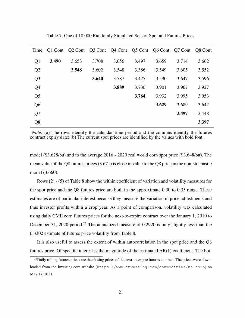
Table 7: One of 10,000 Randomly Simulated Sets of Spot and Futures Prices

Time Q1 Cont Q2 Cont Q3 Cont Q4 Cont Q5 Cont Q6 Cont Q7 Cont Q8 Cont

Q1 3.490 3.653 3.708 3.656 3.497 3.659 3.714 3.662

Q2 3.548 3.602 3.548 3.386 3.549 3.605 3.552

Q3 3.640 3.587 3.425 3.590 3.647 3.596

Q4 3.889 3.730 3.901 3.967 3.927

Q5 3.764 3.932 3.995 3.953

Q6 3.629 3.689 3.642

Q7 3.497 3.448

Q8 3.397

Note: (a) The rows identify the calendar time period and the columns identify the futurescontract expiry date; (b) The current spot prices are identified by the values with bold font.

model ($3.628/bu) and to the average 2016 - 2020 real world corn spot price ($3.648/bu). The

mean value of the Q8 futures prices (3.671) is close in value to the Q8 price in the non-stochastic

model (3.660).

Rows (2) - (5) of Table 8 show the within coefficient of variation and volatility measures for

the spot price and the Q8 futures price are both in the approximate 0.30 to 0.35 range. These

estimates are of particular interest because they measure the variation in price adjustments and

thus investor profits within a crop year. As a point of comparison, volatility was calculated

using daily CME corn futures prices for the next-to-expire contract over the January 1, 2010 to

December 31, 2020 period.22 The annualized measure of 0.2920 is only slightly less than the

0.3302 estimate of futures price volatility from Table 8.

It is also useful to assess the extent of within autocorrelation in the spot price and the Q8

futures price. Of specific interest is the magnitude of the estimated AR(1) coefficient. The bot-

22Daily rolling futures prices are the closing prices of the next-to-expire futures contract. The prices were down-

loaded from the Investing.com website (https://www.investing.com/commodities/us-corn) on

May 17, 2021.

21

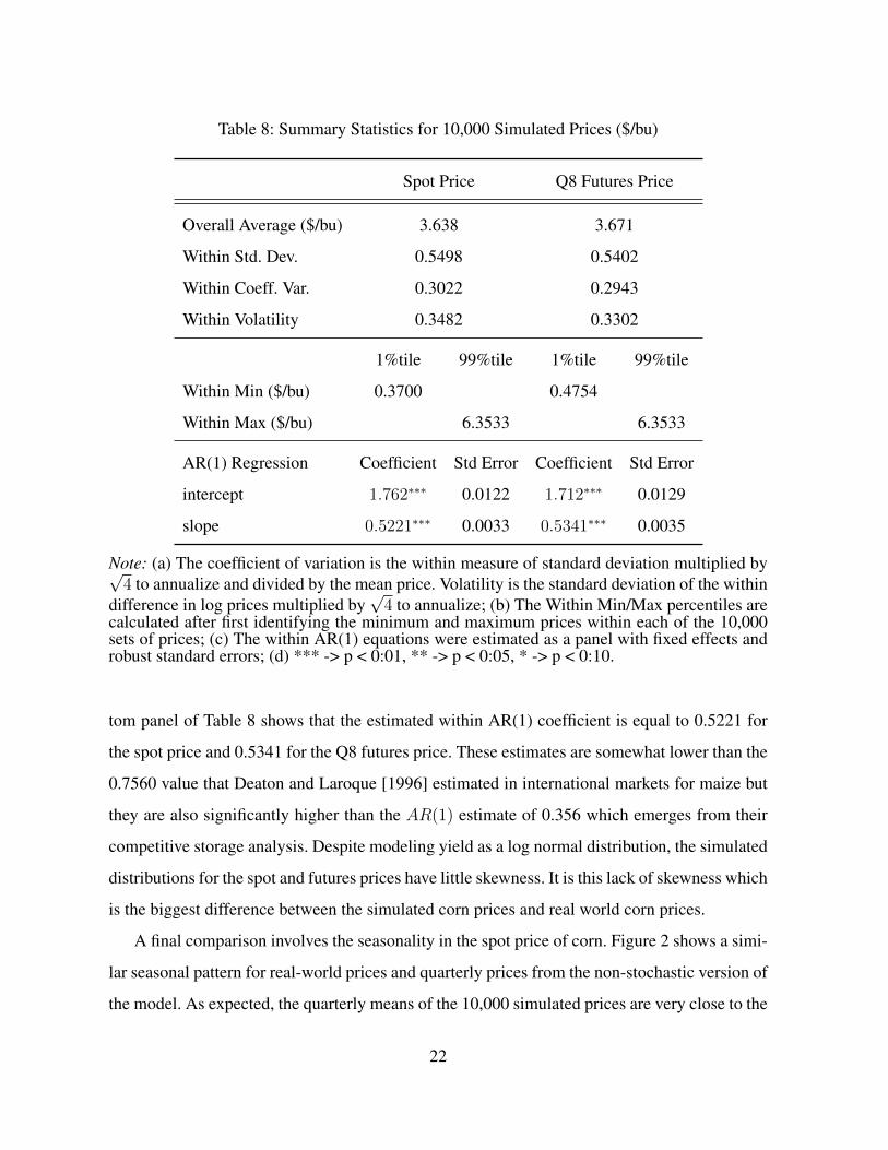
Table 8: Summary Statistics for 10,000 Simulated Prices ($/bu)

Spot Price Q8 Futures Price

Overall Average ($/bu) 3.638 3.671

Within Std. Dev. 0.5498 0.5402

Within Coeff. Var. 0.3022 0.2943

Within Volatility 0.3482 0.3302

1%tile 99%tile 1%tile 99%tile

Within Min ($/bu) 0.3700 0.4754

Within Max ($/bu) 6.3533 6.3533

AR(1) Regression Coefficient Std Error Coefficient Std Error

intercept 1.762∗∗∗ 0.0122 1.712∗∗∗ 0.0129

slope 0.5221∗∗∗ 0.0033 0.5341∗∗∗ 0.0035

Note: (a) The coefficient of variation is the within measure of standard deviation multiplied by√4 to annualize and divided by the mean price. Volatility is the standard deviation of the within

difference in log prices multiplied by√

4 to annualize; (b) The Within Min/Max percentiles arecalculated after first identifying the minimum and maximum prices within each of the 10,000sets of prices; (c) The within AR(1) equations were estimated as a panel with fixed effects androbust standard errors; (d) *** -> p < 0:01, ** -> p < 0:05, * -> p < 0:10.

tom panel of Table 8 shows that the estimated within AR(1) coefficient is equal to 0.5221 for

the spot price and 0.5341 for the Q8 futures price. These estimates are somewhat lower than the

0.7560 value that Deaton and Laroque [1996] estimated in international markets for maize but

they are also significantly higher than the AR(1) estimate of 0.356 which emerges from their

competitive storage analysis. Despite modeling yield as a log normal distribution, the simulated

distributions for the spot and futures prices have little skewness. It is this lack of skewness which

is the biggest difference between the simulated corn prices and real world corn prices.

A final comparison involves the seasonality in the spot price of corn. Figure 2 shows a simi-

lar seasonal pattern for real-world prices and quarterly prices from the non-stochastic version of

the model. As expected, the quarterly means of the 10,000 simulated prices are very close to the

22

quarterly prices in the non-stochastic model (the mean squared error is equal to $0.0000144/bu).

Based on the discussion concerning Figure 2, this implies that the simulated corn prices and the

real-world corn prices have a similar seasonal pattern.

4 Demand Forecast as a Determinant of Investor Profits

This section begins theoretically creating a link between the Q2 outcomes of the two forecast

variables and the expected profits of a commodity-linked investor. The linkage is further illus-

trated by categorizing simulated investor profits according to below and above average values

of the two forecast variables. Theory is then used to create a link between the Q2 outcome of

the two forecast variables and the sign of the Q2 roll yield, and between the sign of the Q2

roll yield and the expected profits for a commodity-linked investor. The simulated outcomes are

then re-categorized into positive and negative values for the net roll yield, which is equivalent to

separating Q2 backwardated market outcomes from Q2 contango market outcomes. The mean

profits for investors within the two categories are compared to confirm the theoretical prediction

that expected profits for the commodity-linked investor are positive in a backwardated market

and negative in a contango market.

4.1 Theoretical Linkage between D2 and Expected Profits

Two alternative measures of expected profits for the long only investor are used in the analysis

below. The "buy-and-hold" measure of profits, which is denoted πhold2,8 , involves the investor in

Q2 taking a long position in a Q8 contract and then offsetting this position after prices have

been established in Q8. The "buy-and-roll" measure of investor profits, which is denoted πroll2,4,8,

involves the investor in Q2 taking a long position in a Q4 contract, offsetting this position in

Q4, immediately taking a long position in a Q8 contract and then offsetting this position in Q8.

Using equation (5), the expected profits for the buy-and-hold investor can be expressed as

E2(πHold2,8 ) = E2(F 88 )− F 8

2 = δ81(E2(H5)− H2) + δ8

2(E2(D8)− D2) (6)

23

The forecast for Q5 production was shown to follow a random walk, which implies H5 =

H2 +eH3 +eH4 +eH5 . The forecast of year 3 net demand was shown to follow an AR(1) stochastic

process of the form Dt = γDt Dt−1 + eDt for t = 4, 5, ..., 8. Recall that because there is no data

for D2 it was assumed that D2 = D3 + eD4 . Using progressive substitution, it can be shown that

D8 =(γD4 ...γ

D8

)D2 +

(γD4 ...γ

D8

)eD3 +

(γD5 ...γ

D8

)eD4

+(γD6 ...γ

D8

)eD5 +

(γD7 γ

D8

)eD6 + γD8 e

D7 + eD8

(7)

After passing through the expectations operator if H5 = H2 + eH3 + eH4 + eH5 and equation (7)

are substituted into equation (6) then the following emerges:

E2(πHold2,8 ) = δ82E2

[(γD4 ...γ

D8

)− 1]D2 (8)

Using the estimate of δ82 = 0.5004 from the solution to the non-stochastic problem together

with the set of values for γDi from Table 6 it can be shown that equation (8) reduces to

E2(πHold2,8 ) = E2(F 88 )− F 8

2 = −0.2174D2 (9)

Notice that equation (9) does not depend on the Q2 forecast of Q5 production. This result

emerges because of the random walk property of the yield forecast. In contrast, equation (9)

shows that expected profits are opposite in sign and proportional to the year 3 net demand

forecast. This result emerges because the econometric estimates imply γD3 ∗ γD4 ∗ ... ∗ γD8 < 1,

which is a necessary condition for a stationary/mean-reverting AR(1) data series.

It is tempting to conclude that mean reversion in the forecast for year 3 net demand causes

mean reversion in the futures price, and it is this mean reversion in the futures price which causes

the expected losses or gains for investors. If this conjecture is true then investors should expected

a negative return when the initial futures price is above average and a positive return if the initial

futures price is below average. With reference to Figure 1 this means that investors should expect

a negative return when investing in the high-priced (June, 2021) backwardated market, and

should expect a positive return when investing in the low-priced (July, 2020) contango market.

The results of this analysis are just the opposite and so in general they cannot be explained by

mean reversion in the futures price.

24

To understand why the expected return is negative with a positive year 3 net demand forecast

and positive with a negative demand forecast it is necessary to focus on the role of stock shifting.

A positive net demand forecast induces a higher rate of storage, which in turn raises the carrying

cost and the Q8 futures price relative to the Q2 spot price. The opposite results emerge with a

forecast of negative net demand. Mean reversion of the demand forecast implies that for an

initial positive demand market the full set of futures prices are expected to gradually weaken

over time, and investors should expect negative profits. Similarly, for an initial negative net

demand market the full set of futures prices are expected to gradually strengthen over time, and

investors should expect positive profits. A gradual weakening or strengthening of the futures

price does not necessarily imply a reversion of the futures price toward its long run value. This

is because although the forecast for Q5 production does not affect the expected rate of change

in the futures price this forecast does determine if the trend line lies above or below the long run

average price. For example, if the Q5 forecast and the year 3 net demand forecast are both high

and the market is in contango, then the set of prices may be below the long term average price,

in which case the gradually weakening prices will be moving away from the long run average

price.

It is also useful to theoretically examine how the expected profits for the buy-and-hold in-

vestor, E2

(πhold2,8

), compare with the expected profits for the buy-and-roll investor, E2

(πroll2,4,8

).

Letting ∆ denote the difference in the two measures of expected profits, equation (5) can be

used to show that

∆ = E2

(πhold2,8

)−E2

(πroll2,4,8

)=(δ8

1 − δ41

) (E2(H4)− H2

)+(δ8

2 − δ42

) (E2(D4)− D2

)(10)

Noting that forecasted production is a random walk it follows that E2(H4) = H2 and thus

the first term on the right side of equation (10) drops out. Regarding the second term, the results

from the non-stochastic model are such that δ82 − δ4

2 = 0.0791. As well, mean reversion of

the net demand forecast implies that E2(D4) − D2 < 0 when D2 > 0 and vice versa. Thus

buy-and-hold results in a larger loss with a positive net demand forecast and a larger gain with

a negative net demand forecast as compared to the buy-and-roll strategy. This result emerges

because the Q8 price impacts are larger than the Q4 price impacts. Consequently, the impacts

25

on profits from the revision in the forecast is smaller with the buy-and-roll strategy since the Q8

contract is not initially included.

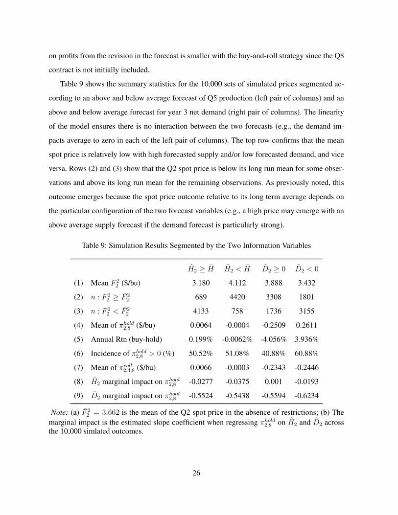
Table 9 shows the summary statistics for the 10,000 sets of simulated prices segmented ac-

cording to an above and below average forecast of Q5 production (left pair of columns) and an

above and below average forecast for year 3 net demand (right pair of columns). The linearity

of the model ensures there is no interaction between the two forecasts (e.g., the demand im-

pacts average to zero in each of the left pair of columns). The top row confirms that the mean

spot price is relatively low with high forecasted supply and/or low forecasted demand, and vice

versa. Rows (2) and (3) show that the Q2 spot price is below its long run mean for some obser-

vations and above its long run mean for the remaining observations. As previously noted, this

outcome emerges because the spot price outcome relative to its long term average depends on

the particular configuration of the two forecast variables (e.g., a high price may emerge with an

above average supply forecast if the demand forecast is particularly strong).

Table 9: Simulation Results Segmented by the Two Information Variables

H2 ≥ H H2 < H D2 ≥ 0 D2 < 0

(1) Mean F 22 ($/bu) 3.180 4.112 3.888 3.432

(2) n : F 22 ≥ F 2

2 689 4420 3308 1801

(3) n : F 22 < F 2

2 4133 758 1736 3155

(4) Mean of πhold2,8 ($/bu) 0.0064 -0.0004 -0.2509 0.2611

(5) Annual Rtn (buy-hold) 0.199% -0.0062% -4.056% 3.936%

(6) Incidence of πhold2,8 > 0 (%) 50.52% 51.08% 40.88% 60.88%

(7) Mean of πroll2,4,8 ($/bu) 0.0066 -0.0003 -0.2343 -0.2446

(8) H2 marginal impact on πhold2,8 -0.0277 -0.0375 0.001 -0.0193

(9) D2 marginal impact on πhold2,8 -0.5524 -0.5438 -0.5594 -0.6234

Note: (a) F 22 = 3.662 is the mean of the Q2 spot price in the absence of restrictions; (b) The

marginal impact is the estimated slope coefficient when regressing πhold2,8 on H2 and D2 acrossthe 10,000 simlated outcomes.

26

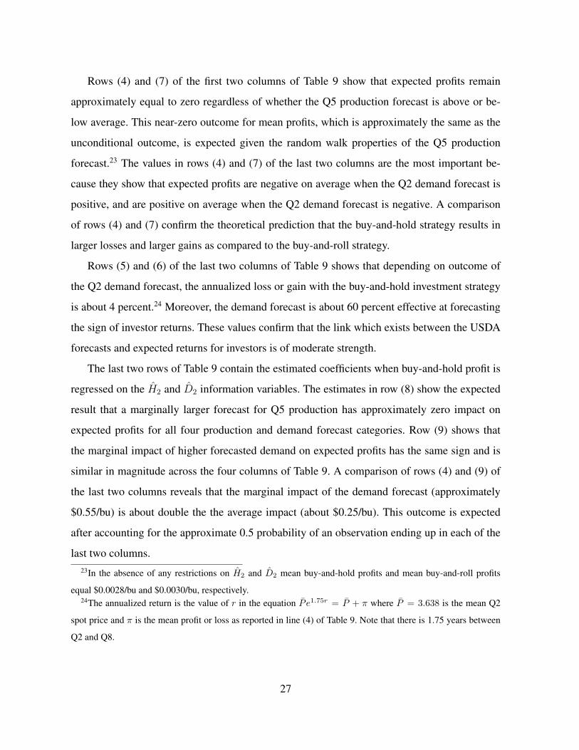
Rows (4) and (7) of the first two columns of Table 9 show that expected profits remain

approximately equal to zero regardless of whether the Q5 production forecast is above or be-

low average. This near-zero outcome for mean profits, which is approximately the same as the

unconditional outcome, is expected given the random walk properties of the Q5 production

forecast.23 The values in rows (4) and (7) of the last two columns are the most important be-

cause they show that expected profits are negative on average when the Q2 demand forecast is

positive, and are positive on average when the Q2 demand forecast is negative. A comparison

of rows (4) and (7) confirm the theoretical prediction that the buy-and-hold strategy results in

larger losses and larger gains as compared to the buy-and-roll strategy.

Rows (5) and (6) of the last two columns of Table 9 shows that depending on outcome of

the Q2 demand forecast, the annualized loss or gain with the buy-and-hold investment strategy

is about 4 percent.24 Moreover, the demand forecast is about 60 percent effective at forecasting

the sign of investor returns. These values confirm that the link which exists between the USDA

forecasts and expected returns for investors is of moderate strength.

The last two rows of Table 9 contain the estimated coefficients when buy-and-hold profit is

regressed on the H2 and D2 information variables. The estimates in row (8) show the expected

result that a marginally larger forecast for Q5 production has approximately zero impact on

expected profits for all four production and demand forecast categories. Row (9) shows that

the marginal impact of higher forecasted demand on expected profits has the same sign and is

similar in magnitude across the four columns of Table 9. A comparison of rows (4) and (9) of

the last two columns reveals that the marginal impact of the demand forecast (approximately

$0.55/bu) is about double the the average impact (about $0.25/bu). This outcome is expected

after accounting for the approximate 0.5 probability of an observation ending up in each of the

last two columns.23In the absence of any restrictions on H2 and D2 mean buy-and-hold profits and mean buy-and-roll profits

equal $0.0028/bu and $0.0030/bu, respectively.24The annualized return is the value of r in the equation P e1.75r = P + π where P = 3.638 is the mean Q2

spot price and π is the mean profit or loss as reported in line (4) of Table 9. Note that there is 1.75 years between

Q2 and Q8.

27

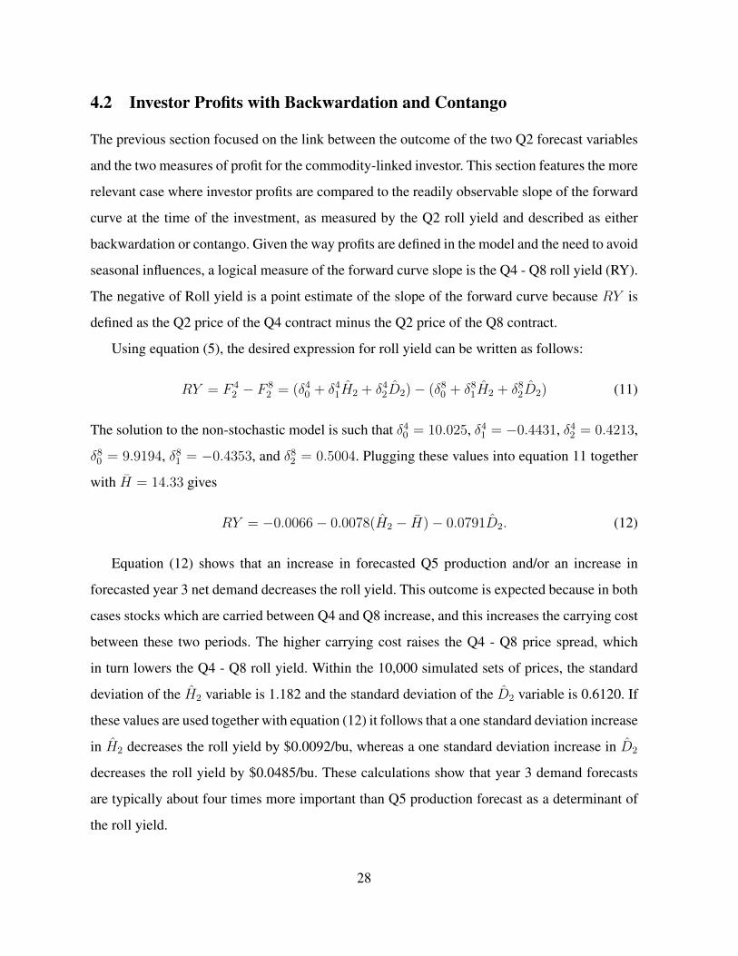
4.2 Investor Profits with Backwardation and Contango

The previous section focused on the link between the outcome of the two Q2 forecast variables

and the two measures of profit for the commodity-linked investor. This section features the more

relevant case where investor profits are compared to the readily observable slope of the forward

curve at the time of the investment, as measured by the Q2 roll yield and described as either

backwardation or contango. Given the way profits are defined in the model and the need to avoid

seasonal influences, a logical measure of the forward curve slope is the Q4 - Q8 roll yield (RY).

The negative of Roll yield is a point estimate of the slope of the forward curve because RY is

defined as the Q2 price of the Q4 contract minus the Q2 price of the Q8 contract.

Using equation (5), the desired expression for roll yield can be written as follows:

RY = F 42 − F 8

2 = (δ40 + δ4

1H2 + δ42D2)− (δ8

0 + δ81H2 + δ8

2D2) (11)

The solution to the non-stochastic model is such that δ40 = 10.025, δ4

1 = −0.4431, δ42 = 0.4213,

δ80 = 9.9194, δ8

1 = −0.4353, and δ82 = 0.5004. Plugging these values into equation 11 together

with H = 14.33 gives

RY = −0.0066− 0.0078(H2 − H)− 0.0791D2. (12)

Equation (12) shows that an increase in forecasted Q5 production and/or an increase in

forecasted year 3 net demand decreases the roll yield. This outcome is expected because in both

cases stocks which are carried between Q4 and Q8 increase, and this increases the carrying cost

between these two periods. The higher carrying cost raises the Q4 - Q8 price spread, which

in turn lowers the Q4 - Q8 roll yield. Within the 10,000 simulated sets of prices, the standard

deviation of the H2 variable is 1.182 and the standard deviation of the D2 variable is 0.6120. If

these values are used together with equation (12) it follows that a one standard deviation increase

in H2 decreases the roll yield by $0.0092/bu, whereas a one standard deviation increase in D2

decreases the roll yield by $0.0485/bu. These calculations show that year 3 demand forecasts

are typically about four times more important than Q5 production forecast as a determinant of

the roll yield.

28

To connect roll yield with expected profits for the commodity-linked investor letRY ∗ denote

the roll yield in excess of RY = −0.0063 where -0.0063 is the roll yield which emerges in

the non-stochastic model (i.e., the neutral forecast roll yield). Solve equation (9) for D2 and

substitute the resulting expression into equation (12) to obtain an expression for expected profits

as function of the net roll yield and the deviation of the Q5 production forecast from its long-run

mean value.

E2

(πhold2,8 |H2, RY

∗) = −0.0214(H2 − H) + 2.748RY ∗ (13)

If the investment decision is conditioned only on the roll yield then within equation (13) the

term H2 − H can be viewed as equivalent to a random error term. With this assumption, the

expectations operator can be passed through equation (13) to get

E2

(πhold2,8 |RH∗) = 2.748RY ∗ (14)

Equation (14) shows the expected profits for the commodity-linked investor as a function

of the net roll yield and with the pair of forecasting variables operating in the background.

The proportionality implies that expected profits are positive for a backwardated market with

a positive net roll yield and are negative for a contango market with a negative net roll yield.

This result is the same as those within the roll yield myth but the reasons are entirely different.

Indeed, in this analysis the roll yield and expected profits are both structurally linked to the

demand forecast. By relegating the demand forecast to the background an implicit link between

the roll yield and investor profits emerges.

In Table 10 the simulation results have been sorted according to the sign and the absolute

size of the net roll yield variable, RY ∗. Row (1) shows that the pair of columns on the left

correspond to weak backwardation (RY ∗ ≥ 0) and weak contango (RY ∗ < 0), respectively.

The pair of columns on the right correspond to strong backwardation and contango, which

requires RY ∗ to be at least one standard deviation above and below zero, respectively. Row (2)

shows that 1,611/10,000 (i.e., ≈ 16%) of the outcomes are strong backwardation and another

≈ 16% are strong contango. Row (3) shows that the conditional roll yield values are rather small

and thus a typical forward curve is not steep, unlike those shown in Figure 1. Keep in mind that

a market may be in contango either because of a high year 3 demand forecast or a high Q5

29

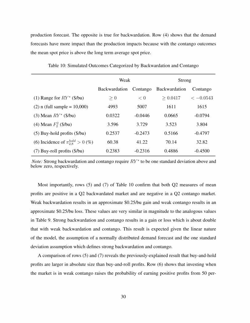
production forecast. The opposite is true for backwardation. Row (4) shows that the demand

forecasts have more impact than the production impacts because with the contango outcomes

the mean spot price is above the long term average spot price.

Table 10: Simulated Outcomes Categorized by Backwardation and Contango

Weak Strong

Backwardation Contango Backwardation Contango

(1) Range for RY ∗ ($/bu) ≥ 0 < 0 ≥ 0.0417 < −0.0543

(2) n (full sample = 10,000) 4993 5007 1611 1615

(3) Mean RY ∗ ($/bu) 0.0322 -0.0446 0.0665 -0.0794

(4) Mean F 22 ($/bu) 3.596 3.729 3.523 3.804

(5) Buy-hold profits ($/bu) 0.2537 -0.2473 0.5166 -0.4797

(6) Incidence of πhold2,8 > 0 (%) 60.38 41.22 70.14 32.82

(7) Buy-roll profits ($/bu) 0.2383 -0.2316 0.4886 -0.4500

Note: Strong backwardation and contango require RY ∗ to be one standard deviation above andbelow zero, respectively.

Most importantly, rows (5) and (7) of Table 10 confirm that both Q2 measures of mean

profits are positive in a Q2 backwardated market and are negative in a Q2 contango market.

Weak backwardation results in an approximate $0.25/bu gain and weak contango results in an

approximate $0.25/bu loss. These values are very similar in magnitude to the analogous values

in Table 9. Strong backwardation and contango results in a gain or loss which is about double

that with weak backwardation and contango. This result is expected given the linear nature

of the model, the assumption of a normally distributed demand forecast and the one standard

deviation assumption which defines strong backwardation and contango.

A comparison of rows (5) and (7) reveals the previously-explained result that buy-and-hold

profits are larger in absolute size than buy-and-roll profits. Row (6) shows that investing when

the market is in weak contango raises the probability of earning positive profits from 50 per-

30

cent to approximately 60 percent. In contrast, investing with strong backwardation raises this

probability to approximately 70 percent.

4.3 False Positives and Negatives

There are obvious advantages of using the readily-observable roll yield to guide investment de-

cisions as opposed to conditioning investments directly on information forecasts. An important

disadvantage is that roll yield investing is subject to false positives and false negatives. Using

equation (12), a false positive occurs when H2 is well below H so thatRY ∗ and D2 both take on

positive values. In this situation the positive roll yield may induce investment but the expected

value of the investment is negative due to the positive value for D2. In contrast, equation ((12)

shows that a false negative occurs when H2 is well above H so that RY ∗ and D2 both take on

negative values. In this case the investment may not take place because of a negative roll yield,

even though the expected value of the investment is positive due to D2 < 0.

In the current analysis the probabilities of false positives and negatives are quite small,

largely because the Q5 production forecast has a relatively weak impact on the slope of the

forward curve. To formally derive this probability substitute RY ∗ − 0.0063 for RY in equation

(12) and then invert the resulting equation to get

D2 = −0.0986(H2 − H)− 12.642RY ∗ (15)

For the case of a false positive, of interest is the probability that D2 > 0 given that RY ∗ > 0.

Further manipulation of equation (15) gives

PROB(D2 > 0) = PROB

(H2 − HσH2

< −128.2

σH2

RY ∗

)(16)

Using an estimate of σH2 = 1.182 from the simulation data, and noting that Φ() is the cu-

mulative distribution function for a standardized normal random variable, equation (16) can be

rewritten as25

PROB(D2 > 0) = Φ (−108.47RY ∗) (17)25To simplify, the analysis in this section assumes that yield follows a normal distribution rather than a log

normal distribution. This assumption changes the results by very little.

31

Suppose the roll yield takes on a small positive value such as RY ∗ = 0.01. Using equation

(17) it can be seen that the probability of a false positive is 10.00 percent. If insteadRY ∗ = 0.02

then the probability of a false positive decreases to 0.5200 percent. The analogous values for a

false negative are of a similar magnitude.

The potential for false positives and negatives suggests that investors should adjust their

investment strategies accordingly. One possibility is for investors to adjust their roll yield in-

vestment threshold according to their general beliefs about Q5 production. For example, if an

investor believes Q5 production is likely to be below average then using the previous analysis

they should guard against a false positive by raising the roll yield trigger. Once again assum-

ing a normal distribution for Q5 production, the expected value of H2 given H2 < H is equal

to 13.38 since this is the mean of a truncated normal distribution, which can be expressed as

µ + 2φ(0)σ. Substituting H2 − H = 13.434 − 14.377 and D2 = 0 into equation (15) gives

RY ∗ = 0.0073. This revised investment threshold is only slightly above the RY ∗ = 0 neutral

forecast investment threshold.

5 Conclusions

A key assumption in this paper is that traders and investors fail to account for the documented

mean reversion in USDA net demand forecasts. The fact that these forecasts are mean reverting

is perhaps not surprising because accounting for a structural supply and demand response during

the forecasting period is likely of secondary concern to the USDA. Mean reversion was shown

to be relatively slow moving and thus likely not obvious to traders. The fact that mean reversion

is slow moving makes the assumption that traders fail to account for this reversion when trading

futures easier to justify. Equation (9) shows that the net demand forecast is expect to change by

about 22 percent (equivalent to about 1 percent per month) over the course of seven quarters.

Despite this small rate of forecast reversion, the impact on investor profits is economically

significant, working out to an annualized gain or loss of about 4 percent on average.

The authors of several of the papers cited in here are clearly frustrated that the roll yield

myth remains firmly entrenched in the minds of many trading professionals. A recent example

32

of this incorrect belief is illustrated by the following set of quotes from a February 9, 2021

Bloomberg commodities post [Luz and Longley, 2021]:

As oil futures power to $60 a barrel, the market’s forward curve has moved sharply

into a pricing pattern where nearer-dated contracts are more expensive than later

ones... The exuberance has helped push holdings of WTI futures to their highest

level since 2018... Roll-yield is a significant driver of commodity futures returns in

the medium- and long-term... The steeper the curve gets, the more interesting it is

for some investors...

Is there any connection between the roll yield myth and the results of this paper? The obvi-

ous connection is that in both cases positive investor returns are most likely with backwardation,

and negative returns are most likely with contango. A second connection is that neither framing

of the problem relies on a change in the risk premium as a source of the investor return. A third

connection is that investors who respond to the roll yield myth will possibly drive futures prices

artificially high when USDA forecasts generate market backwardation. This means that similar

to any bubble scenario, early investors who respond to the USDA-induced roll yield signal may

earn an early-bubble positive return and late investors may earn a late-bubble negative return. A

final connections is that a large scale myth-driven investment response to a positive or negative

roll yield may affect both prices and inventory shifts through time, which in turn may affect the

USDA forecasts of ending stocks and net demand.

An unintended outcome of the current analysis is that it exposes an important weakness

in the price volatility theory of roll yield and excess returns. The price volatility explanation

is compatible with Figure 1, which shows relatively high prices and strong backwardation in

June of 2021, and relatively low prices and strong contango in July of 2020. It is easy to verify

that implied volatility is much higher in the June, 2021 backwardated market than in the July,

2020 contango market. This higher volatility provides theoretical rationale as to why returns are

expected to be higher in a backwardated market.

In contrast to the standard thinking concerning volatility and roll yield, the current analysis

shows that below average stocks and the corresponding high price volatility can emerge in

33

both backwardated markets and contango markets. For example, in the 10,000 simulated sets

of prices, the Q2 stocks variable was below its long term average value 4,891 times, which is

slightly less than 50 percent. During these occurrences the Q2 market was in backwardation

2,647 times (54.12%) and was in contango 2,244 times (45.88%). The result that low stocks

can occur with both market configurations emerges because the relationship between the slope

status of the forward curve (i.e., backwardation versus contango) and the Q2 level of stocks is

non-monotonic. The fact that low stock and the associated higher level of price volatility is not

unique to a backwardated market means that the claimed positive relationship between market

backwardation, the risk premium and investor returns may not be general.

It would be beneficial to test the theoretical hypotheses which were advanced in this paper

using econometric analysis on a data set which combines USDA forecasts and commodity fu-

tures prices, including the full forward curve. Establishing mean reversion in the forecasts is a

straight forward procedure but identifying if the the gain of loss for investors can be attributed

to this mean reversion would be much more challenging. This is because it is likely that a mar-

ket has multiple pricing distortions and isolating one particular distortion will require strong

conditions for identification. Another problem is that futures price data will generally contain

risk premium which are likely to further mask the empirical connection between roll yield and

investor returns which can be attributed to the mean reversion in USDA forecasts.

Perhaps a more relevant extension of the current analysis is to examine how hedgers are

impacted by mean reversion in USDA net demand forecasts. Despite being designed for risk

neutral traders, the model is well suited for examining expected hedging profits and basis risk.

This is because hedging profits depends on the change in the basis over the life of the hedge.

The basis is a special type of roll yield because it is defined as the spot price minus the futures

price. Thus, a USDA market forecast which causes the market to switch from backwardation to

contango and vice versa will necessarily generate gains and losses to short and longer hedgers.

Hedging substitutes basis risk for price risk and an assessment of this risk shifting would be

straight forward to analyze with the current model and data.

34

References

Adjemian, Michael, Philip Garcia, Scott Irwin, and Aaron Smith 2013. Non-convergence in

domestic commodity futures markets: Causes, consequences, and remedies. Economic In-

formation Bulletin 155381, United States Department of Agriculture, Economic Research

Service.

Beck, Stacie E. 1994. Cointegration and market efficiency in commodities futures markets.

Applied Economics 26(3), 249–257.

Bessembinder, Hendrik 2018. The ’roll yield’ myth. Financial Analysts Journal 74(2), 41–53.

Bessembinder, H., J. Coughenour, P. Seguin, and M. Smoller 1995. Mean reversion in equi-

librium asset prices: Evidence from the futures term structure. The Journal of Finance 50,

361–375.

Bhardwaj, Geetesh, Gary Gorton, and Geert Rouwenhorst 2015, June. Facts and fantasies about

commodity futures ten years later. Working Paper 21243, National Bureau of Economic

Research.

Bohl, Martin T., Alexander Putz, and Christoph Sulewski 2020. Speculation and the informa-

tional efficiency of commodity futures markets. Journal of Commodity Markets, in–press.

Bosch, David and Elina Pradkhan 2016. Trading activity and rate of convergence in commodity

futures markets. Journal of Futures Markets 37(9), 930–938.

Breitung, Jorg and Samarjit Das 2005. Panel unit root tests under cross-sectional dependence.

Statistica Neerlandica 59(4), 414–433.

Brennan, Michael J. 1958. The supply of storage. The American Economic Review 48(1),

50–72.

Buccola, Steven T. 1989. Pricing efficiency in agricultural markets: issues, methods and results.

Western Journal of Agricultural Economics 14, 111–121.

35

Carter, Colin A. 2012. Futures and options markets: An introduction (revised). Rebel Publica-

tions: http://www.rebel-publications.com/.

CME 2017, July 10. Trading the curve in energies. Chicago Mercantile Exchange White Paper:

https://www.cmegroup.com/education/whitepapers/trading-the-curve-in-energies.html.

Deaton, Angus and Guy Laroque 1996. Competitive storage and commodity price dynamics.

Journal of Political Economy 104(5), 896–923.

Dewally, Michael, Louis Ederington, and Chitru Fernando 2013. Determinants of Trader Profits

in Commodity Futures Markets. The Review of Financial Studies 26(10), 2648–2683.

Erb, Claude B. and Campbell R. Harvey 2006. The strategic and tactical value of commodity

futures. Financial Analysts Journal 62(2), 69–97.

Fortenbery, T. Randall and Daniel A. Sumner 1993. The effects of usda reports in futures and

options markets. Journal of Futures Markets 13(2), 157–173.

Gorton, Gary and K. Geert Rouwenhorst 2006. Facts and fantasies about commodity futures.

Financial Analysts Journal 62(2), 47–68.

Gorton, Gary B, Fumio Hayashi, and K. Geert Rouwenhorst 2007, July. The fundamentals of

commodity futures returns. Working Paper 13249, National Bureau of Economic Research.

Gorton, Gary B., Fumio Hayashi, and K. Geert Rouwenhorst 2012. The Fundamentals of Com-

modity Futures Returns. Review of Finance 17(1), 35–105.

Harris, Richard D.F. and Elias Tzavalis 1999. Inference for unit roots in dynamic panels where

the time dimension is fixed. Journal of Econometrics 91(2), 201–226.

Im, Kyung So, M Pesaran, and Yongcheol Shin 2003. Testing for unit roots in heterogeneous

panels. Journal of Econometrics 115(1), 53–74.

Irwin, Scott H., Dwight R. Sanders, Aaron Smith, and Scott Main 2020. Returns to investing

in commodity futures: Separating the wheat from the chaff. Applied Economic Perspectives

and Policy 42(4), 583–610.

36

Kaldor, Nicholas 1939. Speculation and economic stability. The Review of Economic Stud-

ies 7(1), 1–27.

Kellard, Neil, Paul Newbold, Tony Rayner, and Christine Ennew 1999. The relative efficiency

of commodity futures markets. Journal of Futures Markets 19(4), 413–432.

Levin, Andrew, Chien-Fu Lin, and Chia-Shang James Chu 2002. Unit root tests in panel data:

asymptotic and finite-sample properties. Journal of Econometrics 108(1), 1–24.

Luz, Andres Guerra and Alex Longley 2021, Feb. 9,. Thirst for yield sees oil market holdings

rocket higher. Bloomberg News, https://ampvideo.bnnbloomberg.ca/thirst-for-yield-sees-oil-

market-holdings-rocket-higher-1.1561220.

McKenzie, Andrew M. and Matthew T. Holt 2002. Market efficiency in agricultural futures

markets. Applied Economics 34(12), 1519–1532.

Moschini, GianCarlo, Harvey Lapan, and Hyunseok Kim 2017. The Renewable Fuel Standard

in Competitive Equilibrium: Market and Welfare Effects. American Journal of Agricultural

Economics 99(5), 1117–1142.

Nordhaus, William D. 1987. Forecasting efficiency: Concepts and applications. The Review of

Economics and Statistics 69(4), 667–674.

Routledge, Bryan R., Duane J. Seppi, and Chester S. Spatt 2000. Equilibrium forward curves

for commodities. The Journal of Finance 55(3), 1297–1338.

Sanders, Dwight R. and Scott Irwin 2012. A reappraisal of investing in commodity futures

markets. Applied Economic Perspectives and Policy 34(3), 515–530.

Symeonidis, Lazaros, Marcel Prokopczuk, Chris Brooks, and Emese Lazar 2012. Futures basis,

inventory and commodity price volatility: An empirical analysis. Economic Modelling 29(6),

2651–2663.

Telser, Lester G. 1958. Futures trading and the storage of cotton and wheat. Journal of Political

Economy 66(3), 233–255.

37

VanEck 2013. Roll yield: No longer the elephant in the room. Van Eck Securities Corpora-

tion: https://vaneck.com/globalassets/home/media/managedassets/library/assets/investment-

cases/cmc-roll-yield-no-longer-the-elephant-in-the-room-sales-idea-2013.pdf.

Williams, Jeffrey C. and Brian D. Wright 1991. Storage and Commodity Markets. Cambridge

University Press.

Working, Holbrook 1948. Theory of the inverse carrying charge in futures markets. Journal of

Farm Economics 30(1), 1–28.

Working, Holbrook 1949. The theory of price of storage. The American Economic Review 39(6),

1254–1262.

38

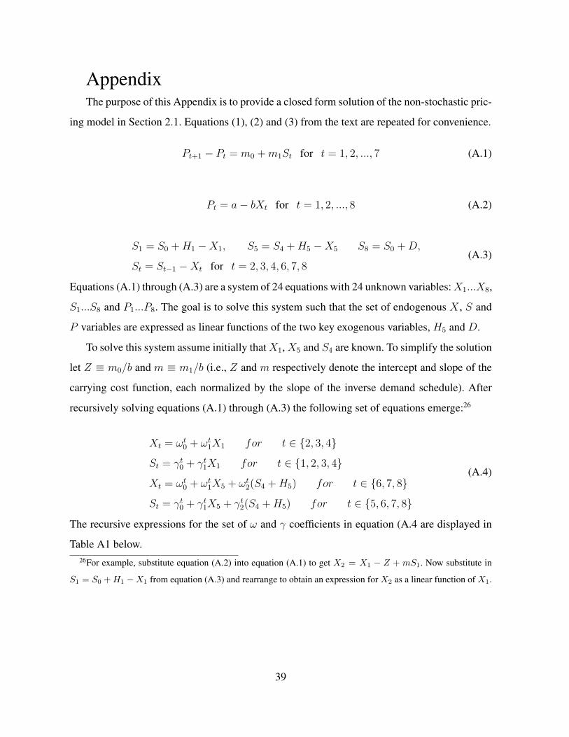
AppendixThe purpose of this Appendix is to provide a closed form solution of the non-stochastic pric-

ing model in Section 2.1. Equations (1), (2) and (3) from the text are repeated for convenience.

Pt+1 − Pt = m0 +m1St for t = 1, 2, ..., 7 (A.1)

Pt = a− bXt for t = 1, 2, ..., 8 (A.2)

S1 = S0 +H1 −X1, S5 = S4 +H5 −X5 S8 = S0 +D,

St = St−1 −Xt for t = 2, 3, 4, 6, 7, 8(A.3)

Equations (A.1) through (A.3) are a system of 24 equations with 24 unknown variables:X1...X8,

S1...S8 and P1...P8. The goal is to solve this system such that the set of endogenous X , S and

P variables are expressed as linear functions of the two key exogenous variables, H5 and D.

To solve this system assume initially thatX1,X5 and S4 are known. To simplify the solution

let Z ≡ m0/b and m ≡ m1/b (i.e., Z and m respectively denote the intercept and slope of the

carrying cost function, each normalized by the slope of the inverse demand schedule). After

recursively solving equations (A.1) through (A.3) the following set of equations emerge:26

Xt = ωt0 + ωt1X1 for t ∈ 2, 3, 4

St = γt0 + γt1X1 for t ∈ 1, 2, 3, 4

Xt = ωt0 + ωt1X5 + ωt2(S4 +H5) for t ∈ 6, 7, 8

St = γt0 + γt1X5 + γt2(S4 +H5) for t ∈ 5, 6, 7, 8

(A.4)

The recursive expressions for the set of ω and γ coefficients in equation (A.4 are displayed in

Table A1 below.26For example, substitute equation (A.2) into equation (A.1) to get X2 = X1 − Z + mS1. Now substitute in

S1 = S0 +H1 −X1 from equation (A.3) and rearrange to obtain an expression for X2 as a linear function of X1.

39

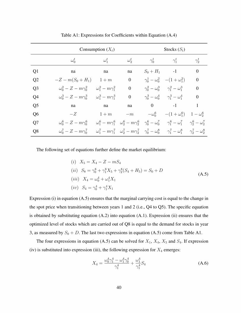
Table A1: Expressions for Coefficients within Equation (A.4)

Consumption (Xt) Stocks (St)

ωt0 ωt1 ωt2 γt0 γt1 γt2

Q1 na na na S0 +H1 -1 0

Q2 −Z −m(S0 +H1) 1 +m 0 γ10 − ω2

0 −(1 + ω21) 0

Q3 ω20 − Z −mγ2

0 ω21 −mγ2

1 0 γ20 − ω3

0 γ21 − ω3

1 0

Q4 ω30 − Z −mγ3

0 ω31 −mγ3

1 0 γ30 − ω4

0 γ31 − ω4

1 0

Q5 na na na 0 -1 1

Q6 −Z 1 +m −m −ω60 −(1 + ω6

1) 1− ω62

Q7 ω60 − Z −mγ6

0 ω61 −mγ6

1 ω62 −mγ6

2 γ60 − ω7

0 γ61 − ω7

1 γ62 − ω7

2

Q8 ω70 − Z −mγ7

0 ω71 −mγ7

1 ω72 −mγ7

2 γ70 − ω8

0 γ71 − ω8

1 γ72 − ω8

2

The following set of equations further define the market equilibrium:

(i) X5 = X4 − Z −mS4

(ii) S8 = γ80 + γ8

1X5 + γ82(S4 +H5) = S0 +D

(iii) X4 = ω40 + ω4

1X1

(iv) S4 = γ40 + γ4

1X1

(A.5)

Expression (i) in equation (A.5) ensures that the marginal carrying cost is equal to the change in

the spot price when transitioning between years 1 and 2 (i.e., Q4 to Q5). The specific equation

is obtained by substituting equation (A.2) into equation (A.1). Expression (ii) ensures that the

optimized level of stocks which are carried out of Q8 is equal to the demand for stocks in year

3, as measured by S0 +D. The last two expressions in equation (A.5) come from Table A1.

The four expressions in equation (A.5) can be solved for X1, X4, X5 and S4. If expression

(iv) is substituted into expression (iii), the following expression for X4 emerges:

X4 =ω4

0γ41 − ω4

1γ40

γ41

+ω4

1

γ41

S4 (A.6)

40

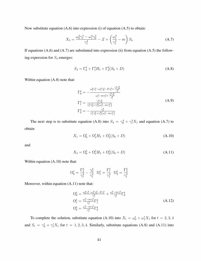
Now substitute equation (A.6) into expression (i) of equation (A.5) to obtain:

X5 =ω4

0γ41 − ω4

1γ40

γ41

− Z +

(ω4

1

γ41

−m)S4 (A.7)

If equations (A.6) and (A.7) are substituted into expression (ii) from equation (A.5) the follow-

ing expression for S4 emerges:

S4 = Γ40 + Γ4

1H5 + Γ42(S0 +D) (A.8)

Within equation (A.8) note that:

Γ40 = −

ω40γ

41−ω4

1γ40−Zγ41+

γ41γ80γ81

ω41−mγ41+

γ41γ82γ81

Γ41 =

γ41γ82

γ41γ82+γ81(ω4

1−mγ41)

Γ42 = − γ41

γ41γ82+γ81(ω4

1−mγ41)

(A.9)

The next step is to substitute equation (A.8) into S4 = γ40 + γ4

1X1 and equation (A.7) to

obtain

X1 = Ω10 + Ω1

1H5 + Ω12(S0 +D) (A.10)

and

X5 = Ω50 + Ω5

1H5 + Ω52(S0 +D) (A.11)

Within equation (A.10) note that:

Ω10 =

Γ42

γ41

− γ40

γ41

Ω11 =

Γ41

γ41

Ω12 =

Γ42

γ41

Moreover, within equation (A.11) note that:

Ω40 =

ω40γ

41−ω4

1γ40−Zγ41

γ41+

ω41−mγ41γ41

Γ40

Ω51 =

ω41−mγ41γ41

Γ41

Ω52 =

ω41−mγ41γ41

Γ42

(A.12)

To complete the solution, substitute equation (A.10) into Xt = ωt0 + ωt1X1 for t = 2, 3, 4

and St = γt0 + γt1X1 for t = 1, 2, 3, 4. Similarly, substitute equations (A.8) and (A.11) into

41

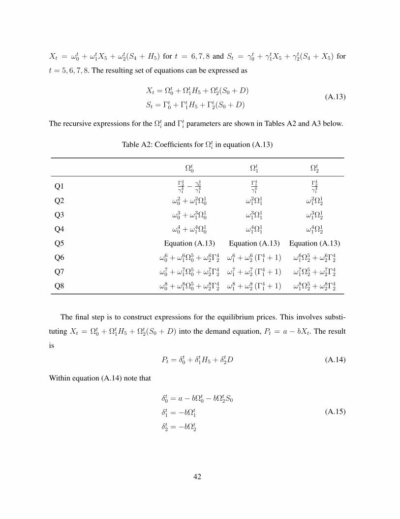
Xt = ωt0 + ωt1X5 + ωt2(S4 + H5) for t = 6, 7, 8 and St = γt0 + γt1X5 + γt2(S4 + X5) for

t = 5, 6, 7, 8. The resulting set of equations can be expressed as

Xt = Ωt0 + Ωt

1H5 + Ωt2(S0 +D)

St = Γt0 + Γt1H5 + Γt2(S0 +D)(A.13)

The recursive expressions for the Ωti and Γti parameters are shown in Tables A2 and A3 below.

Table A2: Coefficients for Ωti in equation (A.13)

Ωt0 Ωt

1 Ωt2

Q1 Γ42

γ41− γ40

γ41

Γ41

γ41

Γ42

γ41

Q2 ω20 + ω2

1Ω10 ω2

1Ω11 ω2

1Ω12

Q3 ω30 + ω3

1Ω10 ω3

1Ω11 ω3

1Ω12

Q4 ω40 + ω4

1Ω10 ω4

1Ω11 ω4

1Ω12

Q5 Equation (A.13) Equation (A.13) Equation (A.13)

Q6 ω60 + ω6

1Ω50 + ω6

2Γ42 ω6

1 + ω62 (Γ4

1 + 1) ω61Ω5

2 + ω62Γ4

2

Q7 ω70 + ω7

1Ω50 + ω7

2Γ42 ω7

1 + ω72 (Γ4

1 + 1) ω71Ω5

2 + ω72Γ4

2

Q8 ω80 + ω8

1Ω50 + ω8

2Γ42 ω8

1 + ω82 (Γ4

1 + 1) ω81Ω5

2 + ω82Γ4

2

The final step is to construct expressions for the equilibrium prices. This involves substi-

tuting Xt = Ωt0 + Ωt

1H5 + Ωt2(S0 + D) into the demand equation, Pt = a − bXt. The result

is

Pt = δt0 + δt1H5 + δt2D (A.14)

Within equation (A.14) note that

δt0 = a− bΩt0 − bΩt

2S0

δt1 = −bΩt1

δt2 = −bΩt2

(A.15)

42

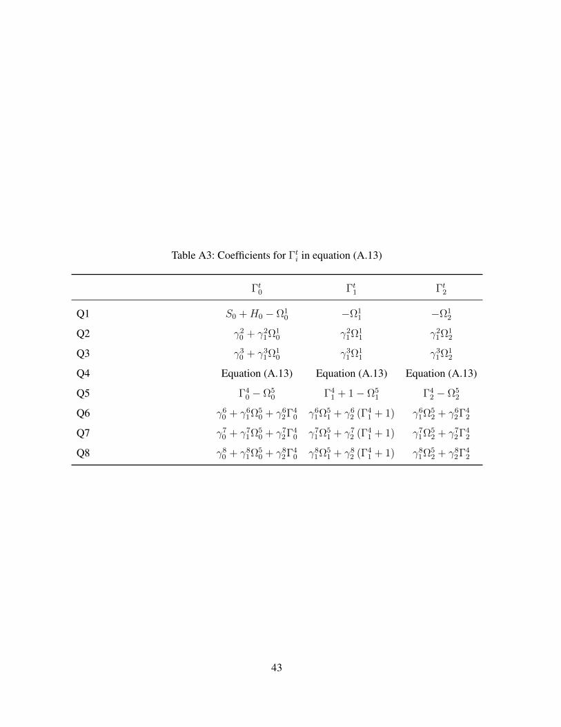
Table A3: Coefficients for Γti in equation (A.13)

Γt0 Γt1 Γt2

Q1 S0 +H0 − Ω10 −Ω1

1 −Ω12

Q2 γ20 + γ2

1Ω10 γ2

1Ω11 γ2

1Ω12

Q3 γ30 + γ3

1Ω10 γ3

1Ω11 γ3

1Ω12

Q4 Equation (A.13) Equation (A.13) Equation (A.13)

Q5 Γ40 − Ω5

0 Γ41 + 1− Ω5

1 Γ42 − Ω5

2

Q6 γ60 + γ6

1Ω50 + γ6

2Γ40 γ6

1Ω51 + γ6

2 (Γ41 + 1) γ6

1Ω52 + γ6

2Γ42

Q7 γ70 + γ7

1Ω50 + γ7

2Γ40 γ7

1Ω51 + γ7

2 (Γ41 + 1) γ7

1Ω52 + γ7

2Γ42

Q8 γ80 + γ8

1Ω50 + γ8

2Γ40 γ8

1Ω51 + γ8

2 (Γ41 + 1) γ8

1Ω52 + γ8

2Γ42

43