bank loan portfolios and the canadian ... - wouter den … loan portfolios and the canadian monetary...

Bank Loan Portfolios and the Canadian Monetary

Transmission Mechanism�

Wouter J. DEN HAAN,y Steven W. SUMNER,z Guy M. YAMASHIROx

May 29, 2008

Abstract

Following a monetary tightening, bank loans to consumers decrease. This is true

both for mortgage and non-mortgage loans, and it is true for a tightening by the

Bank of Canada that is, and is not, a response to a tightening by the Federal Reserve

System. In contrast, business loans typically increase following a monetary tightening.

We argue that the "perverse" response of business loans cannot be explained by an

increase in the demand for funds due to a reduction in real activity. The reason for

this is that we �nd no evidence that business loans increase during a non-monetary

downturn, in which real activity falls and real interest rates do not increase. These

results are consistent with a change in bank portfolio behavior in favor of business

loans in response to an unexpected increase in interest rates.

�The authors would like to thank Francisco Covas and Nicolas Raymond for assistance with obtaining

the Canadian data and Craig Burnside, Zhiwei Zhang and two anonymous referees for useful comments.yDepartment of Economics, University of Amsterdam, Amsterdam, The Netherlands and CEPR, UK.

E-mail: [email protected] of Economics, School of Business, University of San Diego, San Diego, USA.

E-mail: [email protected] of Economics, California State University, Long Beach, USA.

E-mail: [email protected].

1 Introduction

There is a large empirical literature documenting that monetary policy shocks a¤ect eco-

nomic activity.1 In particular, empirical studies estimated over di¤erent time periods and

using data from di¤erent countries indicate that an unexpected monetary tightening is

followed by a (delayed) reduction in real activity.2 Understanding the transmission mech-

anism remains a challenge, however, and in particular, the importance of the banking

system in accentuating the transmission to the real economy is still unclear.

Proponents of a �bank-lending channel�hold that a monetary tightening should be fol-

lowed by a decline in the supply of bank loans, which exacerbates the economic downturn.

It is our position that examining the role of the banking system in the transmission mech-

anism requires understanding the portfolio behavior of banks. In particular, additional

insights can be gained by looking at the behavior of bank loan components as opposed to

looking at just total bank loans. In Den Haan, Sumner, and Yamashiro (2007), we �nd

support for this position using U.S. data. Our speci�c �ndings are as follows. First, the

behavior of total loans is consistent with that of a bank-lending and/or interest-rate chan-

nel. That is, total loans decrease more during a downturn caused by a monetary tightening

than during downturns of comparable magnitude that are not triggered by a monetary

policy shock. Second, following a monetary tightening there is a strong shift out of real

estate and consumer loans and into commercial and industrial (business) loans resulting

in an increase in commercial and industrial loans. During non-monetary downturns of

comparable magnitude, however, we �nd no such increases in commercial and industrial

(C&I) loans, which suggests that the increase in C&I loans is not due to an increase in

the demand for such loans because of the drop in real activity. Our �ndings, therefore,

support the existence of a bank-lending channel, but only in relation to consumer and real

estate loans. In fact, the results suggest that the shift out of these types of loans following

1See Bernanke and Gertler (1995) and Christiano, Eichenbaum, and Evans (1999) for detailed discus-

sions on how economic variables respond following a monetary policy shock. See Duguay (1994) for a

discussion on the monetary transmission mechanism in Canada.2Cecchetti (1999), for example, documents that output decreases in all of the eleven OECD countries

considered.

a monetary tightening allows for an increase in the supply of commercial and industrial

loans.

That business loans may increase following a monetary tightening is also documented

in Gertler and Gilchrist (1993). Moreover, Bernanke and Gertler (1995) argue that the

"perverse response" can be explained by an increase in the demand for these loans. Our

results indicate, however, that the observed increase is more likely the result of an increase

in the supply. The idea that the supply of commercial and industrial loans increases

following a monetary tightening is clearly a contentious �nding. While the theoretical

literature in support of the bank-lending channel typically focuses on the supply of loans

to �rms,3 we �nd no empirical evidence of the bank-lending channel operating through this

type of loan. Our empirical results do, however, provide support for the recent upsurge

in theoretical papers emphasizing the role of �nancing imperfections in the consumer loan

market in business cycle analysis.4

The obvious question is whether our surprising �ndings are speci�c to the U.S., or

whether they are found in other countries as well. In this paper, we seek to answer this

question by investigating whether the portfolio behavior of Canadian banks following a

monetary tightening is the same as that of U.S. banks. Using data for the Canadian

economy is especially revealing because the Canadian economy and banking system di¤er

in fundamental aspects from the U.S. economy and banking system. In particular, the

Canadian economy is much more open than the U.S. economy, and the Canadian banking

system is comprised of only a handful of large banks, whereas the U.S. system includes

more than 7,000 banks including many smaller banks. Despite these di¤erences, we �nd

that the results for Canadian bank loans are remarkably similar to those found using U.S.

data.

This study di¤ers in the following two aspects from Den Haan, Sumner, and Yamashiro

(2007) in which we use U.S. data. First, in our Canadian data set, real estate lending is

broken down into loans to businesses (commercial real estate) and loans to consumers

(residential real estate). This distinction is not made in the U.S. data. This is important

3See, for example, Fisher (1999) and Repullo and Suarez (2000).4See, for example, Campbell and Hercowitz (2004) and Iacoviello (2005).

2

because it sheds light on whether the change in the banks�loan portfolios is one mainly

out of real estate (or long-term) loans into short-term loans, or whether it is a shift from

loans to consumers to loans to businesses. Our results suggest it is the latter. The second

di¤erence with Den Haan, Sumner, and Yamashiro (2007) is that we consider two types of

monetary downturns. The �rst monetary downturn is a tightening by the Bank of Canada

(BoC) that is not a response to a tightening by the Federal Reserve System (FED) and

the second monetary downturn is a tightening by the Bank of Canada that is a response

to a FED tightening

The remainder of the paper is organized as follows. Section 2 highlights the similarities

and di¤erences in the �nancial systems of the U.S. and Canada. Section 3 discusses the

data used and the empirical methodology. Section 4 presents the results and the last

section concludes.

2 U.S. and Canadian �nancial systems

While there are many similarities between the �nancial systems in the United States and

Canada there are also many di¤erences. It is, therefore, interesting to see whether the

remarkable results found with U.S. data are present in Canadian data as well. Monetary

policy in both countries focuses on the economic and �nancial well-being of the country

with a primary goal of maintaining price stability. Both countries currently target a short-

term interest rate representing the rate at which �nancial institutions can borrow and lend

funds with one another. Furthermore, to promote transparency in monetary policy, both

countries have eight ��xed�dates at which they make announcements regarding the target

policy variable.5 The main di¤erence between the countries in terms of monetary policy

is that the Bank of Canada maintains an explicit operating target range for in�ation of

1-3% per year based on total CPI (since 1991), whereas the Board of Governors of the

Federal Reserve System does not.

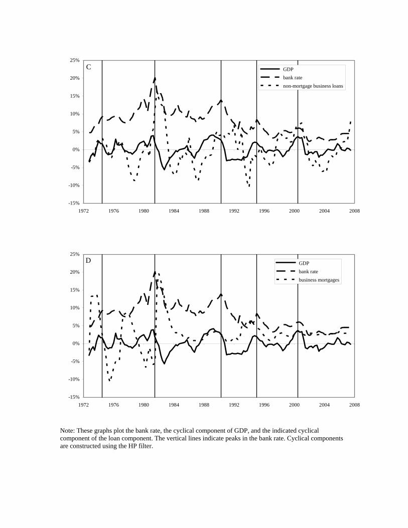
Low-frequency changes in the composition of banks� loan portfolios are also similar

in the two countries. Figure 1 plots the shares of the four loan series for Canada over

5This began in Canada in 2001 and in the U.S. in 1996.

3

our sample from the fourth quarter of 1972 to the third quarter of 2007. It shows that

consumer real estate loans have become relatively more important, growing from 19% in

the �rst ten years of the sample to just over 50% of total loans in the last ten years of

the sample. In contrast, the share of business loans has decreased sharply from 54% in

the �rst ten years to 24% in the last ten years. Consumer loans have remained fairly

constant. Real estate loans to �rms are only a small part of the banks�loan portfolio, but

their share has grown substantially, from less than 1% to around 3%. The data for U.S.

loan components display similar (but not identical) trends. As in Canada, commercial

and industrial loans start out as the most important loan component but is overtaken by

real estate loans. In the U.S. this happens in 1987, just a couple years before the same

thing happened in Canada.6 One di¤erence is that in the U.S. the fraction of consumer

loans displays a gradual drop from 25% to 16% of total loans.

Despite these similarities there are also some important di¤erences that could a¤ect

the responses of the di¤erent loan components following a monetary tightening. The U.S.

banking system consists of many small- and medium-sized commercial banks, whereas the

Canadian banking system is dominated by a few large commercial banks. In particular,

as of January 2008 there are over 7000 commercial banks operating in the U.S. and only

20 domestic banks in Canada.7 Canadian banks compete, however, with other �nancial

companies such as life insurance companies and mutual fund companies that themselves

face tough competition in their primary market.8 In the U.S. these various �nancial

services are dominated by a few large nationwide companies. Moreover, Canadian banks

have been less restricted, not only with respect to the setting of interest rates,9 but they

also had a wider business scope and the ability to branch nationwide throughout the

sample. The larger number of smaller banks and the historical obstacles to nationwide

6Based on H.8 data downloaded from the website of the Federal Reserve System.7From the website of the Canadian Banking Association.8Allen and Engert (2007) summarize di¤erences in performance of Canadian and U.S. banks and discuss

the amount of competition in the Canadian banking market.9Canada did not have an interest rate ceiling on deposits, while in the U.S. interest rate ceilings on

deposits and savings accounts (Regulation Q) were only abolished in the 1980s.

4

banking in the U.S. have fostered relationship lending.10 Relationship lending may a¤ect

the desire and ability of banks to protect their customers during a monetary tightening

when their own source of funds are becoming scarcer and more expensive.

We discuss two additional reasons why U.S. banks may be better capable of sheltering

their business customers from the negative e¤ects of monetary tightening. The �rst reason

is related to the mortgage market. Courchane and Giles (2002), report that even though

home ownerships rates are similar (67% in the U.S. and 64% in Canada in 2000), di¤er-

ences in public policy objectives resulted in di¤erences in housing and mortgage markets.

Canada�s policies have focused more on direct schemes to acquire and retain housing,

whereas in the U.S., the focus has been on ensuring a supply of funds for mortgage lend-

ing. As a result, until recently, the variety of mortgages o¤ered in the U.S. was greater

than that being o¤ered in Canada. In general terms, Canada had mortgages with shorter

maturities, lower loan-to-value ratios, and interest rates that were not tax deductible.11

Long-term mortgages are not attractive when interest rates rise, for example, because

they put current-pro�t margins under pressure, which, in turn, makes it more di¢ cult to

have a su¢ ciently high capital adequacy ratio. This means that banks with long-term

mortgages, i.e. U.S. banks, may want to substitute out of mortgages, which would free up

resources to lend to �rms. The public policy objectives pursued in the U.S. resulted in a

strong secondary market for mortgages. Freedman (1998) documents that securitization

of mortgages started much earlier in the U.S. and is of much less importance in Canada.

The presence of a strong secondary market for mortgages would make it easier for U.S.

banks to unload mortgages.

The second reason relates to composition of banks� loan portfolios. Although the

qualitative trends in the banks�portfolio composition has been similar there are important

di¤erences in the levels. In particular, Canadian (non-mortgage) business loans dropped

from 57% of total loans in 1972Q4 to 19% in 2007Q3, whereas U.S. (non-mortgage) business

loans dropped from 42% to 25%. Faced with stronger long-term shifts out of business loans

it may be less important for Canadian banks to safeguard business loans when interest

10See, for example, Berger and Udell (1995) and Petersen and Rajan (1994,1995).11See Courchane and Giles (2002).

5

rates increase.

Above we provided three reasons why it could be more important and/or easier for

U.S. banks not to reduce business loans during a monetary tightening. But there is one

reason why business loans should fall by less in Canada. Because Canadian �rms are

more dependent on bank loans, a reduction in bank lending has the potential to be much

more harmful. Freedman (1998) documents that the share of business credit raised through

bonds is roughly half that raised through bank loans. In the U.S., the fraction of corporate

bonds and commercial paper to bank loans and (bank and non-bank) mortgages was equal

to 90% in 2003.12 But if it is harder for Canadian banks to get funds from other types

of �nancial institutions then demand factors may prevent bank loans from dropping in

Canada following a monetary tightening.

3 Data and empirical methodology

In this section, we discuss the data and the empirical methods used. In particular, we

show how to estimate the behavior of variables during a monetary downturn (in Section

3.3) and during a non-monetary downturn (in Section 3.4).

3.1 Data sources

All data used are from Statistics Canada. Because not all of the data is available on a

monthly basis, we use quarterly data over a sample period, which begins with the fourth

quarter of 1972 and extends through the third quarter of 2007. The four bank loan series

are: non-mortgage consumer loans, residential mortgages (consumer mortgages), non-

mortgage business loans, and non-residential mortgages (business mortgages). We focus

attention only on loans held by domestic banks. As of January 2005, domestic banks held

94% of mortgages, 93% of non-mortgage loans, and 93% of total assets (OFSI website,

author calculation). We augment this data with the Bank of Canada bank rate, taken to

12Using data from Table L.101 of the Flow of Funds for non-�nancial business.

6

be the indicator of the monetary authority,13 the consumer price index, and gross domestic

product. A more detailed description of the data is provided in the Appendix.

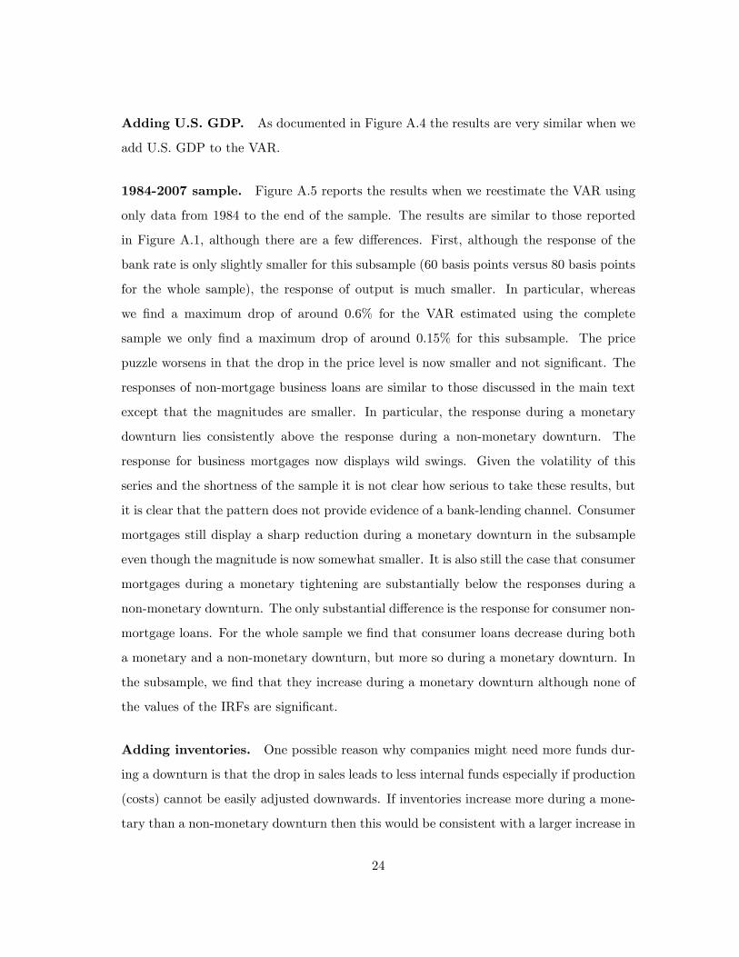
3.2 Behavior of the loan components

In this section, we describe the time series behavior of the loan components. Each panel of

Figure 2 plots detrended real GDP, the interest rate, and the indicated loan component.

There are �ve episodes in which the interest rate clearly reaches (local) peaks. Those

are the seventies, early eighties, early nineties, mid nineties, and the beginning of the

millennium. The �gure documents that each episode (indicated in the graph with a vertical

line) is followed by a period in which GDP is below its trend value, although after the

interest rate hike of the mid nineties the cyclical component of GDP is only slightly

negative. The di¤erent loan components behave di¤erently in the periods following these

interest rate hikes. Panel A documents that the cyclical component of non-mortgage

consumer loans� like the cyclical component of GDP� is negative for some time following

an interest rate hike, although after the interest rate hike of the mid nineties only with some

delay. As documented in Panel B, the behavior for consumer mortgages is similar. Again,

there are �ve periods of negative detrended values, each corresponding to an interest rate

hike. The correlation between the cyclical component of GDP and non-mortgage consumer

loans is equal to 0.71 and with consumer mortgages it is slightly less, equal to 0.59.

Results are very di¤erent for business loans. First, consider the behavior of non-

mortgage business loans in Panel C. In order to associate the periods in which the de-

trended loan series are negative with interest rate hikes one would have to use long and

13Following the explicit targeting of a short-term interest rate by central banks, the recent literature

typically only considers an interest rate as the monetary policy indicator even though interest-rate targeting

may not have been in place throughout the entire sample. The appropriate interest rate to use as the

monetary policy instrument for Canada would be the call loan (or overnight) rate. We use the bank rate,

however, because it is available for a longer period and its behavior follows the overnight rate closely when

both are available. Racette and Raynauld (1992) and Racette, Raynauld, and Sigouin (1994) use the

prime corporate paper rate as the relevant policy instrument. Reestimation of our system using the prime

corporate rate as well as reestimation over the shorter sample using the call loan rate leads to very similar

results.

7

variable delays. An easier way to describe the comovement of interest rates and non-

mortgage business loans is the following. At the start of each of the �ve interest rate

hikes, non-mortgage business loans are at a trough (relative to its trend values), but then

increase together with the interest rate and decline (possibly with some delay) when the

interest rate declines. The behavior during the early eighties is especially remarkable in

that non-mortgage business loans even follows the temporary loosening of monetary policy

in the middle of 1980. The correlation of the detrended loan component and GDP is only

0.08.

Panel D plots the results for mortgage business loans. This loan component is only a

small fraction of total bank lending but it grew rapidly over the sample period. Some of

the rapid growth bursts that took place in the �rst half of the sample are not taken out by

the �lter. Thus, one should be careful when interpreting these results. Nevertheless, some

interesting lessons can be drawn. In particular, following the sharp monetary tightening

of the eighties, real estate lending to �rms sharply increased. It is possible that this sharp

increase (which was not reversed in the un�ltered data) is better modeled as a change in

the trend. Whether the increase is due to a change in the trend or a change in the cyclical

component, it is still remarkable that it occurred following a monetary tightening, a period

after which� at least according to the conventional view� the supply of bank loans should

decrease.

The discussion in this section simply points at some comovements during particular

episodes. Below, we show that this informal discussion is con�rmed with the results

obtained using the empirical methodology described in the remainder of this section.

3.3 Two types of monetary downturns

The standard procedure to study the impact of monetary policy on economic variables

is to estimate a structural VAR using a limited set of variables. Consider the following

8

VAR:14

Zt = B1Zt�1 + � � �+BqZt�q +D0rffrt + � � �+Dqrffrt�q + ut; (1)

where Z 0t = [X01t; rt; X

02t], X

01t is a (k1 � 1) vector, with elements whose contemporaneous

values are in the information set of the central bank, rt is the monetary policy variable

(bank rate), X 02t is a (k2� 1) vector with elements whose contemporaneous values are not

in the information set of the central bank, and ut is a (k � 1) vector of residual terms

with k = k1 + 1 + k2. rffrt is the federal funds rate which is assumed to be una¤ected by

Canadian variables. We further assume that all lagged values are in the information set

of the central bank. In order to proceed, one has to assume that there is a relationship

between the reduced-form error terms, ut, and the fundamental, or structural, shocks to

the economy, "t. We assume that this relationship is given by:

ut = A"t; (2)

where A is a (k � k) matrix of coe¢ cients and "t is a (k � 1) vector of fundamental

uncorrelated shocks, each with a unit standard deviation. Thus,

E�utu

0t

�= AA0: (3)

When we replace E [utu0t] by its sample analogue, we obtain k(k + 1)=2 conditions on the

coe¢ cients in A. Since A has k2 elements, k(k � 1)=2 additional restrictions are needed

to estimate all elements of A. A standard procedure is to obtain the additional k(k� 1)=2

restrictions by assuming that A is a lower-triangular matrix. Christiano, Eichenbaum, and

Evans (1999), however, show that to determine the e¤ects of a monetary policy shock one

can work with the less-restrictive assumption that A has the following block -triangular

structure:

A =

26664A11 0k1�1 0k1�k1

A21 A22 01�k2

A31 A32 A33

37775 ; (4)

14To simplify the expressions we do not display constants, trend terms, and seasonal dummies that are

included in the empirical implementation.

9

where A11 is a (k1 � k1), A21 is a (1� k1) matrix, A31 is a (k2 � k1), A22 is a scalar, A32is a (k2 � 1), A33 is a (k2 � k2), and 0i�j is a matrix with zero elements. Note that this

structure is consistent with the assumption made above about the information set of the

central bank.

Our benchmark speci�cation is based on the assumption that X2t is empty and that

all other elements are, thus, in X1t. Intuitively, X2t being empty means that the central

bank responds to contemporaneous innovations in all of the variables of the system.15 It

also means that none of the variables can respond contemporaneously to monetary policy

shocks. We impose the same restriction on changes in the federal funds rate. That is,

all elements of the (k � 1) vector D are assumed to be equal to zero except the element

corresponding to the Canadian bank rate. In other words, we allow the Canadian central

bank to respond contemporaneously to unexpected changes in the federal funds rate. This

structure allows us to consider two di¤erent types of monetary downturns.

FED initiated monetary downturn. The �rst type of monetary downturn is a mon-

etary downturn that is initiated by the FED. We use the impulse response function of the

federal funds rate from Den Haan, Sumner, and Yamashiro (2007), which is obtained by

estimating a VAR with U.S. data, to pin down the size of the shock and the time path

along which the federal funds rate returns back to normal. An increase in the federal funds

rate leads to an increase in the Canadian bank rate in the same period, but a¤ects other

Canadian variables only in the next period.

Bank of Canada initiated monetary downturn. The second type of monetary down-

turn is initiated by the Bank of Canada. This is a response to the (k1 + 1)th element of

". Since the equation of the Canadian bank rate includes both the contemporaneous and

lagged values of the federal funds rate, this change in the Canadian bank rate is not a

response to a FED change in the interest rate.

15The results are similar under the alternative assumption that the monetary authority does not respond

to contemporaneous innovations of the other variables in the system.

10

3.4 Non-monetary downturns

The impulse response functions for the monetary downturns not only re�ect the direct

responses of the variables to an increase in the interest rate, but also the indirect responses

to changes in the other variables and, in particular, to the decline in real activity. This

makes it di¢ cult to understand what is going on, especially since a decline in real activity

could increase or decrease the demand for bank loans.16 For example, an increase in a loan

component during a monetary downturn could still be consistent with a credit crunch,

if the decline in real activity strongly increases the demand for that loan component.

Thus, without the credit crunch this loan component would have increased even more. To

�lter out this indirect e¤ect of real activity, we compare the behavior of loan components

during a monetary downturn with their behavior during a non-monetary downturn of

equal magnitude. While a monetary downturn is caused by a monetary tightening, a

non-monetary downturn is caused by one or more output shocks.

There are two schemes to construct non-monetary downturns. In the �rst scheme, the

structural shock is simply the innovation to output from the reduced-form VAR. For our

purposes, it is not that important to interpret the nature of this structural shock. The

key feature, however, is that while this shock decreases real activity it does not lead to

an increase in interest rates.17 It, therefore, distinguishes itself from a monetary shock in

a fundamental way. We mainly focus on a second scheme that is similar to the �rst but

ensures that the behavior of output during a non-monetary downturn is identical to that

observed during a monetary downturn. This makes it convenient to quantitatively compare

the responses during the two types of downturns. According to this second scheme, a non-

monetary downturn is caused by a sequence of output shocks such that output follows the

exact same path as it does during a monetary downturn. As documented in the appendix,

16On one hand, the reduction in real activity would reduce investment and, thus, the need for loans,

while on the other hand the reduction in internal cash �ow could increase the demand for loans. The latter

would especially manifest itself if production cannot easily be scaled down so that a reduction in sales

leads to an increase in inventories.17We �nd that output shocks lead to reductions in the interest rate but they are quantitatively very

small.

11

the responses of the loan components following a single output shock tell a story that is

very similar to that implied by the loan components responses during a non-monetary

downturn (following a sequence of output shocks).18

With output declining during both downturns the key di¤erence between the two is the

behavior of the interest rate. Thus, the di¤erence between the impulse response functions

for the loan variables of the monetary and the non-monetary downturn can be interpreted

as the e¤ect of the increase in the interest rate holding real activity constant. That

is, by comparing the behavior of the loan variables during a monetary downturn with

that observed during a non-monetary downturn, we �lter out the changes in demand and

supply that are caused by the reduction in output. Obviously, there are pitfalls to this

comparison, but we think that they provide a useful set of contrasting empirical results.

3.5 Speci�cation of the VARs and standard errors

Each VAR includes one year of lagged variables, a constant, a linear trend, and quarterly

dummies to adjust the data for seasonality.19 The coe¢ cients are estimated with ordinary

least squares (OLS) and the signi�cance levels are established using a Monte Carlo proce-

dure with 5,000 replications in which data are generated by bootstrapping the estimated

residuals. To avoid clutter we do not report con�dence bands in the graphs but instead

use open and solid squares to indicate that an estimate is signi�cant at the 10% and 5%

level, respectively.20

18 Implementing these exercises requires us to make an additional assumption on A. In particular, we

assume that the only shock that a¤ects real activity is this "output" shock. That is, the matrix A11 also

has a block-triangular structure. Note that the block-triangular structure imposed in Equation 4 already

made the assumption that any structural shock, including the monetary shock, could have an e¤ect on

the monetary policy variable, but that the monetary shock only had an immediate e¤ect on the monetary

policy variable.19We include seasonal dummies because non-residential mortgages are not seasonally adjusted.20Signi�cance levels are for one-sided tests.

12

4 Results

FED initiated monetary downturn. In this section, we examine a monetary tight-

ening that is induced by the FED. In particular, we consider the responses of Canadian

variables (including the bank rate) when the federal funds rate increases and then follows

the time path indicated by the estimated impulse response function of Den Haan, Sumner,

and Yamashiro (2007). Panels A through C of Figure 3 plot the responses of the bank

rate, the price level, and real GDP following this FED tightening. The bank rate closely

follows the federal funds rate but increases by a smaller amount. The peak increase in

the federal funds rate is equal to 81 basis points, whereas the peak response in the bank

rate is equal to 61 basis points. It is typically assumed that at least part of the increase

in the nominal rate is due to an increase in the real rate. Bhuiyan and Lucas (2007)

document� using Canadian data� that this is indeed the case. In particular, they show

that an increase in the overnight target rate by 22 basis points leads to an increase in the

ex ante real rate (of a one-year bond) by 18 basis points and a decrease in the expected

in�ation rate by 5 basis points. Real GDP drops signi�cantly for over a year reaching its

maximum decline of 0.58% after approximately 2 years. The response of the price level

indicates that our results su¤er from the price puzzle, but the puzzle is much smaller here

than in other papers; the price level experiences a small (but signi�cant) increase during

the �rst few years, after which it displays a more substantial (but insigni�cant) decline

below its original level.21 Moreover, as documented below we do not face the price puz-

zle when we consider a tightening that is not initiated by the FED, and for alternative

speci�cations discussed in the appendix the price puzzle is even less apparent than it is

in Figure 3.22 Fung and Kasumovich (1998) resolve the price puzzle for several countries

including Canada using long-run restrictions. Barth and Ramey (2001) and Gaiotti and

Secchi (2004) argue, however, that an increase in the price level is not a puzzle, because

21 In contrast, Den Haan, Sumner, and Yamashiro (2007) �nd using U.S. data a strong signi�cant increase

in the price level that is not followed by a substantial decline.22Fung and Gupta (1997) �nd using Canadian data a strong signi�cant increase in the price level when

monetary tightenings are identi�ed as negative innovations to a liquidity variable, but their price response

is similar to ours when monetary shocks are identi�ed as innovations to an interest rate.

13

increases in the interest rate could lead to an increase in the price level through a cost

channel. Given that there are reasons why the price level should not fall following a mone-

tary innovation, and since we only face a modest price puzzle, we would rather not search

for that particular speci�cation, which delivers the desired result for prices.

Figures 3A and 3B also plot the behavior of the bank rate and the price level during

a non-monetary downturn in which the changes in output are identical to those observed

following a monetary tightening (Figure 3C), but are instead caused by a sequence of

output shocks. The �gure shows that interest rates decrease somewhat in response to the

negative output shocks, but that the reduction is very small. Prices display a moderate

drop during a non-monetary downturn.

Panels D through G of Figure 3 plot the responses of the four loan components after

a positive innovation in the federal funds rate. The key observation is that� as is the

case for the loan components of U.S. banks� the components behave very di¤erently.

Non-mortgage consumer loans and consumer mortgages display a gradual and persistent

decline. The decline in these two loan components follow the drop in output but their

declines last longer. The magnitudes are also larger. The maximum drop of non-mortgage

consumer loans is equal to 1.78% and the maximum drop of consumer mortgages is equal

to 2.23%, more than triple the fall of output. Results not shown indicate that consumer

loans behave similarly to total loans.

Both types of business loans behave di¤erently from consumer loans. Following a

monetary tightening, both display sharp increases that are signi�cant at the 10% level

in the �rst quarter and signi�cant at the 5% level for several subsequent quarters. Non-

mortgage business loans return to their original level roughly four years following the shock

after which they display a moderate but signi�cant decline. Business mortgages remain

high for an even longer time period.

Non-monetary downturn (corresponding to FED initiated downturn). To shed

some light on the question of how the downturn in real activity, following the monetary

contraction, a¤ects the loan components, we also analyze the responses of the loan com-

ponents during a non-monetary downturn in which the path of output is exactly as it

14

is during the monetary downturn. Recall that interest rates barely move during such a

downturn.

Non-mortgage consumer loans decline in response to output shocks but the decline

during the non-monetary downturn is roughly half that of the decline during a comparable

monetary downturn. For consumer mortgages the di¤erence is even greater. Whereas

consumer mortgages sharply decline during a monetary tightening, they are virtually �at

during a non-monetary downturn. How the non-monetary downturn is constructed is not

important, since the same qualitative results are found when responses following a single

output shock are considered.23

The behavior of both types of consumer loans during a monetary, thus, �ts the text-

book story of a monetary tightening. That is, loans decrease and they decrease by more

than what can be explained by the reduction in real activity. In contrast, the behavior

of both types of business loans does not �t the textbook story about the monetary trans-

mission mechanism. Consider the behavior of non-mortgage loans to �rms. Above we

mentioned that this type of loan displays a sharp increase during a monetary downturn.

During a non-monetary downturn, however, they display a signi�cant decline although the

decline is modest (roughly half the drop in output). Similarly, business mortgages, while

increasing during a monetary downturn, are basically unchanged during a non-monetary

downturn. Since a reduction in real activity could lead to either a decrease in the demand

for loans (since investment decreases) or an increase (since internal �nancing decreases),

the observed reduction in business loans following the negative output shocks is not that

surprising. But if a reduction in real activity leads to a reduction in loans during a

non-monetary downturn, then why do loans to businesses increase during a monetary

downturn? We return to this question in the last section.

Bank of Canada initiated monetary downturn In this section, we consider an

increase in the Bank of Canada bank rate that is not a response to an increase in the

federal funds rate. The correlation between the bank and the federal funds rate is high,

namely 88% for our quarterly data, but even when we allow the federal funds rate to

23See the appendix.

15

a¤ect the bank rate contemporaneously, we �nd substantial innovations to the bank rate.

The results are given in Figure 4. Panel A documents that the monetary tightening that

is initiated by the Bank of Canada corresponds to increases in the bank rate that are

similar to those that are observed when the increases are in response to a FED tightening.

The same is true for the drop in output. The response for the price level is somewhat

di¤erent and the price puzzle now has clearly disappeared. The price level is basically

�at for roughly two years after which it displays a gradual and persistent decline, that is

signi�cant at the 5% level.

We now turn to the responses of the loan components. Qualitatively the responses of

the two types of consumer loans following a tightening initiated by the Bank of Canada are

very similar to those observed when the downturn is initiated by the FED. Quantitatively,

however, the drops are much smaller. This suggests that Canadian banks may be better

able to shelter their portfolio of consumer loans when interest rates only increase in Canada

and not the United States.

Whether the interest rate increase is due to a tightening initiated by the FED or the

Bank of Canada also does not matter for the qualitative results for business mortgages,

although, it does matter for non-mortgages business loans. When the increase in the

interest rate is due to a tightening initiated by the FED, non-mortgage business loans

display a sharp and persistent increase. When the increase is initiated by the Bank

of Canada, we �nd a similar initial increase after which the impulse response function

becomes negative but insigni�cant.24 The explanation for this result may be related to the

one given to explain the smaller responses in consumer loans. In the last section, we argue

that it is very well possible that the sharp reductions in consumer mortgages and other

consumer loans that are observed when interest rates increase in both Canada and the U.S.

occur because these loans are less attractive to banks when interest rates increase. This

substitution out of consumer loans frees up resources that can be used to increase business

loans. But if Canadian banks can obtain funding for their loans in the U.S. at lower rates,

then consumer loans may not be as unattractive. Therefore, if consumer loans decrease

24There are some signi�cant values after �ve years but these should probably not be taken seriously.

16

by less then there is less room for business loans to increase. An alternative explanation

is that demand for business loans is lower during a monetary downturn initiated by the

Bank of Canada, because Canadian �rms would rather borrow from U.S. lenders than

from Canadian lenders when the interest di¤erential between Canadian and U.S. rates

increases.

Non-monetary downturn (corresponding to BoC initiated downturn). Since

the output decline following a tightening initiated by the Bank of Canada is very similar

to the output decline following a FED tightening, it is also the case that the responses

during the two non-monetary downturns are very similar. But since quantitatively (and

for non-mortgage business loans also qualitatively) the results are di¤erent during the two

monetary downturns it will be useful to do another comparison.

Although the decline in consumer mortgages is milder when the increase in the interest

rate is due to an independent tightening by the Bank of Canada, the response during

non-monetary downturns is �at, which means that the behavior of these loans is still

consistent with the textbook description of a monetary tightening. The smaller decline

in non-mortgage consumer loans does change the interpretation since consumer loans do

decrease during a non-monetary downturn. In fact, as documented in Panel D of Figure

4, the declines in non-mortgage consumer loans during a monetary and a non-monetary

downturn are now quite similar. These results are consistent with the hypothesis that

when interest rates increase in Canada but not in the U.S., the reduction in non-mortgage

consumer loans is due to the drop in real activity and not to the increase in the interest

rate.

Business mortgages also increase during a monetary downturn initiated by the Bank

of Canada. Since they do not increase during a non-monetary downturn, they clearly do

not �t the standard textbook story. Finally, we discuss non-mortgage business loans. The

signi�cant initial increase in non-mortgage business loans clearly cannot be explained by

the decline in real activity. Interestingly, except for this initial decrease non-mortgage

business loans closely follow the behavior of non-mortgage business loans during a non-

monetary downturn, which is exactly what we found for non-mortgage consumer loans.

17

To summarize, when interest rates increase in Canada but not in the U.S., the behavior

of non-mortgage loans (both business and consumer loans) is very similar to that observed

during downturns of equal magnitude caused by a series of output shocks instead of a

monetary shock. For mortgage loans, it is less important whether the tightening is initiated

by the FED and followed by the Bank of Canada or whether the tightening only occurs

in Canada.

Robustness Exercises. In the appendix, we show that the results are robust to several

modi�cations. In particular, we do the following. We calculate the impulse response

functions using a standard VAR that does not distinguish between a tightening initiated

by the Bank of Canada and a FED tightening. The results are basically an average of

the ones reported here for the two types of monetary downturns. We also show that the

results are robust to adding the exchange rate, U.S. GDP, and business inventories to the

VAR. When we add inventories we generate the non-monetary downturn using output and

inventory shocks so that we match both the response of output and inventories observed

during the monetary downturn. We also reestimate the VAR using only more recent data

and �nd similar responses for most variables. Finally, we document that the responses

for the non-monetary downturns (which are based on a sequence of output shocks) are

qualitatively similar to the responses observed after a single output shock.

We also tried alternative assumptions about the number of lags and trend speci�cations

and found that the results are robust.25

5 Concluding comments

The responses of Canadian loans to a monetary tightening initiated by the FED� and

followed by the bank of Canada� are remarkably similar to those found for the U.S. econ-

omy. In particular, both types of consumer loans decrease during a monetary downturn

and they decrease by much more than during a comparable non-monetary downturn. In

25These results can be found through the link "robustness: di¤erent trend & lag structures" on

http://www1.fee.uva.nl/toe/content/people/content/denhaan/papers.html.

18

contrast, business loans increase following the increase in interest rates while we do not

observe such an increase during a non-monetary downturn.

The responses following a tightening initiated by the Bank of Canada, which leaves

U.S. interest rates unchanged, are similar but there are also some di¤erences. The decline

in real activity is almost identical across the two types of monetary downturns. Although

consumer loans decrease during both monetary downturns, the decrease in non-mortgage

consumer loans during a tightening initiated by the Bank of Canada can be fully explained

by the reduction in real activity. Except for the initial rise, the same is true for non-

mortgage business loans. For mortgages, however, the rise in Canadian interest rates

clearly has an e¤ect that is not explained by the decline in real activity independent of

which central bank initiates the tightening.

Given that business loans do not increase following a series of negative output shocks,

the increase in business loans following a monetary tightening is unlikely to be caused by

the reduction of real activity. It is not impossible that an increase in interest rates leads to

an increase in the demand for loans if the higher burden of interest payments can only be

met by increased borrowing. But if �rms are in such dire need of extra funds, the question

arises as to why banks are willing to supply the extra funds.

There are several reasons why banks may want to adjust their loan portfolio following

a monetary tightening. One possibility is that the risk of loans to consumers increases by

far more than the risk of loans to �rms. This would shift the portfolio towards business

loans, and if the portfolio shift is strong enough then the supply of business loans could

even increase. Minetti (2007) develops a model in which banks a¤ect the risk of their �rm

loans with the amount they lend out. In such an environment banks may want to give

priority to business lending because a reduction in the amount lent to a �rm may increase

the risk and lower expected returns.26 Another possibility considered is a shift from long-

term (i.e., real estate) loans towards short-term loans. The idea is that the increase in the

short-term rate decreases the current-period pro�t margin on long-term loans. If banks

26But note that this motivation should only be present during a monetary downturn because we do not

see during a non-monetary downturn.

19

worry about the book value of their equity position then such a reduction in bank pro�ts

may induce banks to move out of long-term loans into short-term loans.27

With our U.S. data set we were unable to distinguish between real estate loans to

consumers and �rms. Using Canadian data, our empirical �nding that both types of

business loans (mortgages and non-mortgage loans) increase when interest rates increase

in both Canada and the U.S., suggests that it is the type of borrower and not so much the

type of loan that matters. That is, our results suggest that consumers are more likely than

�rms to be constrained during a monetary downturn. The conclusion that consumers and

not businesses are credit constrained is consistent with the results of Safaei and Cameron

(2003).28 Although the theoretical literature on agency costs in �nancing has typically

focused on loans to �rms, there are now several papers that build dynamic business cycle

models in which frictions associated with lending to consumers play a crucial role.29 Our

empirical results document that especially following a monetary tightening consumers are

more likely than �rms to be constrained and, thus, make clear the importance of theoretical

work that emphasizes frictions in consumer �nance.

Another aspect of our results that deserve more attention is the following. Our em-

pirical work focuses on banks� loan portfolios following a monetary tightening. We do

not address what happens to other types of funding30 and whether these changes in the

27One such reason could be regulation such as the Basel accord. Den Haan, Sumner, and Yamashiro

(2007) argue that even before the Basel accord was implemented there were reasons for banks to safeguard

their equity position.28They �nd in response to a monetary policy shock, a positive comovement between output and credit,

both when credit to businesses and when credit to persons is used. In response to a positive "credit supply

shock," however, output increases when bank credit to persons is used but output decreases when bank

credit to businesses is used. The latter is consistent with the pattern we �nd during a monetary downturn.

Note that while we do not separately identify a credit supply shock� which requires a complex set of

restrictions� it is possible that our monetary policy shock captures, in part, a credit supply shock like the

one identi�ed in Safaei and Cameron (2003).29See, for example, Campbell and Hercowitz (2004) and Iacoviello (2005).30 It is possible that the increase in bank funding makes up for a decline in funding from other sources.

This raises the question why banks are not ful�lling this role during a non-monetary downturn while they

are capable of doing it following a monetary tightening.

20

bank loan portfolios are important in magnifying or propagating the e¤ects of the mon-

etary tightening. Whether, for example, the observed reduction in consumer mortgages

is important in a¤ecting investment in real estate depends on alternative �nancing pos-

sibilities. This is obviously a di¢ cult question, but Iacoviello and Minetti (2007) make

progress on this issue by investigating whether shocks to the ratio of non-bank mortgages

to bank mortgages a¤ect house prices. Using data for Finland, Germany, Norway, and

the U.K. they �nd mixed results and they argue that the di¤erences can be explained by

di¤erences in the mortgage markets such as the depth of the funding system, the presence

of a diversi�ed range of mortgage lenders, and the ability to share credit risk.

A Appendix

A.1 Data Sources

All Canadian data series are from Statistics Canada, while U.S. data series are from the

St. Louis FED FRED database.

� Bank rate (v122530). Quarterly series are constructed using the average of the

monthly observations.

� Total Consumer Price Index (v735319). Quarterly series are constructed using the

average of the monthly observations.

� (Non-mortgage) business loans (v122645). Quarterly series are constructed using

the average of the monthly observations.

� Business mortgages (v122656). Quarterly series are constructed using the average

of the monthly observations.

� (Non-mortgage) consumer loans (v122709). Quarterly series are constructed using

the average of the monthly observations.

� Consumer mortgages (v122748). Quarterly series are constructed using the average

of the monthly observations.

21

� Gross Domestic product (v499686). Quarterly data.

� Federal funds rate. Quarterly series are constructed using the average of the monthly

observations.

B Robustness

We performed the following robustness exercises.

1. Estimate a standard VAR that does not distinguish between a monetary tightening

initiated by the FED and the bank of Canada.

2. Report the results to a single output shock.

3. Add the exchange rate to the VAR.

4. Add U.S. GDP to the VAR.

5. Reestimate the results using only the more recent data.

6. Add inventories to the VAR and consider a non-monetary downturn in which output

and inventory shocks are such that the implied response for output and the implied

response for inventories is identical to the one observed during a monetary downturn.

The data sources for the additional data are the following.

� Inventories (v1992058), Statistics Canada. Quarterly level series are constructed

using the quarterly change series.

� Exchange rate, FRED. Quarterly series are constructed using the average of the

monthly observations.

� U.S. GDP, FRED. Quarterly data.

22

Results using a standard VAR. Figure A.1 plots the results when we use a standard

VAR in which we do not include the federal funds rate. In this speci�cation, an innovation

in the bank rate captures both a response to a change in the federal funds rate as well

as an independent tightening by the Bank of Canada. The results are similar to those

reported in the main text for a tightening initiated by the FED. But quantitatively they are

actually somewhat smaller, that is, they are best described as an average of the downturns

initiated by the FED and the Bank of Canada. The only thing that is somewhat di¤erent is

that during a non-monetary downturn consumer mortgages actually display a signi�cant

increase. This is also found by Den Haan, Sumner, and Yamashiro (2007) and only

increases the gap between the response during a monetary and a non-monetary downturn.

Responses following a single output shock. As discussed in Section 3.4, the re-

sponses of variables during a non-monetary downturn are the responses to a series of

output shocks (this made it possible to get an identical output response during the two

di¤erent downturns). The responses of the variables during a non-monetary downturn

are, however, qualitatively very similar to the responses to a single output shock. This is

documented in Figure A.2, which plots the responses of output and the loan components

following a one-time negative output shock.

First, note that following an output shock the initial output response is larger than

the one constructed for the non-monetary downturn in Figure A.1, but the dynamic path

is not that di¤erent. It still has a slight hump shape, and after roughly three years it has

returned back to its original level. As was observed during a non-monetary downturn,

non-mortgage consumer loans decline and consumer mortgages increase. Business loans

also move in the same direction as observed during a non-monetary downturn, except that

in response to a single output shock business mortgages initially display an (insigni�cant)

increase.

Adding the exchange rate. As documented in Figure A.3 the results are very similar

when we add the exchange rate to the VAR.

23

Adding U.S. GDP. As documented in Figure A.4 the results are very similar when we

add U.S. GDP to the VAR.

1984-2007 sample. Figure A.5 reports the results when we reestimate the VAR using

only data from 1984 to the end of the sample. The results are similar to those reported

in Figure A.1, although there are a few di¤erences. First, although the response of the

bank rate is only slightly smaller for this subsample (60 basis points versus 80 basis points

for the whole sample), the response of output is much smaller. In particular, whereas

we �nd a maximum drop of around 0.6% for the VAR estimated using the complete

sample we only �nd a maximum drop of around 0.15% for this subsample. The price

puzzle worsens in that the drop in the price level is now smaller and not signi�cant. The

responses of non-mortgage business loans are similar to those discussed in the main text

except that the magnitudes are smaller. In particular, the response during a monetary

downturn lies consistently above the response during a non-monetary downturn. The

response for business mortgages now displays wild swings. Given the volatility of this

series and the shortness of the sample it is not clear how serious to take these results, but

it is clear that the pattern does not provide evidence of a bank-lending channel. Consumer

mortgages still display a sharp reduction during a monetary downturn in the subsample

even though the magnitude is now somewhat smaller. It is also still the case that consumer

mortgages during a monetary tightening are substantially below the responses during a

non-monetary downturn. The only substantial di¤erence is the response for consumer non-

mortgage loans. For the whole sample we �nd that consumer loans decrease during both

a monetary and a non-monetary downturn, but more so during a monetary downturn. In

the subsample, we �nd that they increase during a monetary downturn although none of

the values of the IRFs are signi�cant.

Adding inventories. One possible reason why companies might need more funds dur-

ing a downturn is that the drop in sales leads to less internal funds especially if production

(costs) cannot be easily adjusted downwards. If inventories increase more during a mone-

tary than a non-monetary downturn then this would be consistent with a larger increase in

24

the demand for business loans after a monetary than a non-monetary downturn. To check

this hypothesis we add the change in inventories to our VAR and rede�ne a non-monetary

downturn as a downturn caused by output and inventory shocks such that the responses

of output and inventories are identical to those observed after a monetary tightening.

Adding inventories to the VAR leaves the impulse response functions of a monetary

tightening reported in Figure A.1 almost una¤ected. Only the response of business loans

is a little bit lower. When we look at an inventory shock then we �nd� in contrast to

our results for the U.S.� that inventories decrease following a monetary downturn. Since

business loans drop following a negative inventory shock, this means that business loans

drop even more during a non-monetary downturn, when a non-monetary downturn is

de�ned as a downturn in which output and investment shocks generate a time path for

output and inventories identical to that observed during a monetary downturn. These

�ndings are documented in Figure A.6 that plot the response of non-mortgage business

loans during both a monetary and a non-monetary downturn.

References

[22] Allen, Jason, and Walter Engert, 2007, E¢ ciency and competition in Canadian Bank-

ing, Bank of Canada Review Summer, 33-45.

[22] Barth, Marvin J., and Valerie A. Ramey, 2001, The cost channel of monetary trans-

mission, NBER Macroeconomics Annual 16, 199-239.

[22] Berger, Allen N., and Gregory F. Udell, 1995, Relationship lending and lines of credit

in small �rm �nance. Journal of Business 63, 351-381.

[4] Bernanke, Ben S., and Mark Gertler, 1995, Inside the black box: The credit channel

of monetary policy transmission, Journal of Economic Perspectives 9, 27-48.

[5] Bhuiyan, Rokon, and Robert F. Lucas, 2007, Real and nominal e¤ects of monetary

policy shocks, Canadian Journal of Economics 40, 679-702.

25

[6] Campbell, Je¤rey R., and Zvi Hercowitz, 2004, The role of collateralized household

debt in macroeconomic stabilization, Federal Reserve Bank of Chicago working paper

WP 2004-24.

[7] Cecchetti, Stephen G., 1999, Legal structure, �nancial structure, and the monetary

policy transmission mechanism, FRBNY Economic Policy Review July, 9-28.

[8] Christiano, Lawrence J., Martin Eichenbaum, and Charles Evans, 1999, Monetary

policy shocks: What have we learned and to what end?, in Handbook of Macroeco-

nomics, John B. Taylor and Michael Woodford (eds.), North Holland, Amsterdam.

[9] Courchane, Marsha J., and Judith A. Giles, 2002, A comparison of U.S. and Canadian

residential mortgage markets, Property Management 20, 326-368.

[22] Den Haan, Wouter J., Steven W. Sumner, and Guy M. Yamashiro, 2007, Bank loan

portfolios and the monetary transmission mechanism, Journal of Monetary Economics

54, 904-924.

[11] Duguay, Pierre, 1994, Empirical evidence on the strength of the monetary transmis-

sion mechanism in Canada, Journal of Monetary Economics 33, 39-61.

[12] Fisher, Jonas D.M., 1999, Credit market imperfections and the heterogeneous re-

sponse of �rms to monetary shocks, Journal of Money, Credit and Banking 31, 187-

211.

[22] Freedman, Charles, 1998, The Canadian banking system, Bank of Canada Technical

Report 81.

[14] Fung, Benedict S.C., and Rohit Gupta, 1997, Cash setting, the call loan rate, and

the liquidity e¤ect in Canada, Canadian Journal of Economics 30, 1057-1082.

[22] Fung, Ben Siu-cheong Fung, and Marcel Kasumovich, 1998, Monetary shocks in the

G-6 countries: Is there a puzzle? Journal of Monetary Economics 42, 575-592.

26

[22] Gaiotii, Eugenio, and Alessandro Secchi, 1996, Is there a cost channel of monetary

policy transmission? An investigation into the pricing behavior of 2,000 �rms, Journal

of Money, Credit, and Banking 38, 2013-2037.

[17] Gertler, Mark, and Simon Gilchrist, 1993, The role of credit market imperfections

in the monetary transmission mechanism: Arguments and evidence, Scandinavian

Journal of Economics 95, 43-64.

[18] Iacoviello, Matteo, 2005, House prices, borrowing constraints and monetary policy in

the business cycle, American Economic Review 95, 739-764.

[19] Iacoviello, Matteo, and Raoul Minetti, 2007, The credit channel of monetary policy:

evidence from the housing market, forthcoming in Journal of Macroeconomics.

[22] Minetti, Raoul, 2007, Bank capital, �rm liquidity, and project quality, Journal of

Monetary Economics 54, 2584-2594.

[22] Petersen, Mitchell A., and Raghuram G. Rajan, 1994, The bene�ts of lending rela-

tionships: evidence from small business data, Journal of Finance 49, 3-37.

[22] Petersen, Mitchell A., and Raghuram G. Rajan, 1995, The e¤ect of credit market

competition on lending relationships, Quarterly Journal of Economics 110, 407-443.

[23] Racette, Daniel, and Jacques Raynauld, 1992, Canadian monetary policy: will the

check-list approach ever get us to price stability?, Canadian Journal of Economics

25, 819-838.

[24] Racette, Daniel, Jacques Raynauld, and Christian Sigouin, 1994, An up-to-date and

improved BVAR model of the Canadian economy, Working paper WP-94-4, Bank of

Canada, Ottawa.

[25] Repullo, Rafael, and Javier Suarez, 2000, Entrepreneurial moral hazard and bank

monitoring: A model of the credit channel, European Economic Review 44, 1931-

1950.

27

[26] Safaei, Jalil, and Norman E. Cameron, 2003, Credit channel and credit shocks in

Canadian macrodynamics �a structural VAR approach, Applied Financial Economics

13, 267-277.

28

Figure 1: Loan components as a fraction of total loans

0%

10%

20%

30%

40%

50%

60%

1972 1976 1980 1984 1988 1992 1996 2000 2004 2008

non-mortgage business loans

consumer mortgage loans

non-mortgage consumer loans

business mortgage loans

Figure 2: Interest rate and cyclical components of GDP and loan components

-15%

-10%

-5%

0%

5%

10%

15%

20%

25%

1972 1976 1980 1984 1988 1992 1996 2000 2004 2008

GDP bank rate non-mortgage consumer loans

A

-15%

-10%

-5%

0%

5%

10%

15%

20%

25%

1972 1976 1980 1984 1988 1992 1996 2000 2004 2008

GDP bank rate consumer mortgages

B

-15%

-10%

-5%

0%

5%

10%

15%

20%

25%

1972 1976 1980 1984 1988 1992 1996 2000 2004 2008

GDP bank rate non-mortgage business loans

C

-15%

-10%

-5%

0%

5%

10%

15%

20%

25%

1972 1976 1980 1984 1988 1992 1996 2000 2004 2008

GDP bank rate business mortgages

D

Note: These graphs plot the bank rate, the cyclical component of GDP, and the indicated cyclical component of the loan component. The vertical lines indicate peaks in the bank rate. Cyclical components are constructed using the HP filter.

Figure 3: Responses during a monetary and a non-monetary downturn Tightening initiated by the FED

-0.25

0.00

0.25

0.50

0.75

1.00

0 1 2 3 4 5 6 7

time (years)

: 10% significance level: 5% significance level

monetary downturn

non-monetary downturn

A Bank rate and U.S. FFR

Federal Funds Rate: U.S. monetary contraction

-0.75%

-0.65%

-0.55%

-0.45%

-0.35%

-0.25%

-0.15%

-0.05%

0.05%

0.15%

0.25%

0 1 2 3 4 5 6 7

time (years)


monetary downturn


B Price level

-0.75%

-0.65%

-0.55%

-0.45%

-0.35%

-0.25%

-0.15%

-0.05%

0.05%

0.15%

0.25%

0 1 2 3 4 5 6 7

time (years)


C Real GDP

-2.00%

-1.50%

-1.00%

-0.50%

0.00%

0.50%

0 1 2 3 4 5 6 7

time (years)


monetary downturn


D Non-mortgage Consumer

-2.50%

-2.00%

-1.50%

-1.00%

-0.50%

0.00%

0.50%

0 1 2 3 4 5 6 7

time (years)


monetary downturn


E Consumer mortgages

-1.00%

-0.50%

0.00%

0.50%

1.00%

1.50%

2.00%

0 1 2 3 4 5 6 7

time (years)

: 10% significance level: 5% significance levelmonetary downturn


F Non-mortgage business

-2.50%

-1.50%

-0.50%

0.50%

1.50%

2.50%

3.50%

4.50%

0 1 2 3 4 5 6 7

time (years)


monetary downturn


G Business mortgages

Note: The graphs plot the responses to a monetary policy shock of the FED (FED monetary downturn) and the responses to a sequence of output shocks that result in the same responses for real output (FED non-monetary downturn).

Figure 4: Responses during a monetary and a non-monetary downturn Bank of Canada tightening that is not a response to FED tightening

-0.25

-0.15

-0.05

0.05

0.15

0.25

0.35

0.45

0.55

0.65

0.75

0 1 2 3 4 5 6 7

time (years)


monetary downturn


A Bank rate

-0.50%

-0.40%

-0.30%

-0.20%

-0.10%

0.00%

0.10%

0 1 2 3 4 5 6 7

time (years)



B Price level

-0.70%

-0.60%

-0.50%

-0.40%

-0.30%

-0.20%

-0.10%

0.00%

0.10%

0 1 2 3 4 5 6 7

time (years)


C Real GDP

-1.25%

-1.05%

-0.85%

-0.65%

-0.45%

-0.25%

-0.05%

0.15%

0 1 2 3 4 5 6 7

time (years)


monetary downturn



-1.10%

-0.90%

-0.70%

-0.50%

-0.30%

-0.10%

0.10%

0 1 2 3 4 5 6 7

time (years)


monetary downturn



-0.50%

-0.40%

-0.30%

-0.20%

-0.10%

0.00%

0.10%

0.20%

0.30%

0.40%

0.50%

0 1 2 3 4 5 6 7

time (years)


monetary downturn



-1.75%

-1.25%

-0.75%

-0.25%

0.25%

0.75%

1.25%

1.75%

2.25%

2.75%

0 1 2 3 4 5 6 7

time (years)




Note: The graphs plot the responses to a one-standard-deviation monetary policy shock of the Bank of Canada (BoC monetary downturn) and the responses to a sequence of output shocks that result in the same responses for real output (BoC non-monetary downturn).

Figure A.1: Responses during a monetary and a non-monetary downturn No distinction between Bank of Canada and FED tightening

-0.40

-0.20

0.00

0.20

0.40

0.60

0.80

1.00

0 1 2 3 4 5 6 7

time (years)


monetary downturn


A Bank rate

-0.50%

-0.40%

-0.30%

-0.20%

-0.10%

0.00%

0.10%

0.20%

0 1 2 3 4 5 6 7

time (years)


monetary downturn


B Price level

-0.70%

-0.60%

-0.50%

-0.40%

-0.30%

-0.20%

-0.10%

0.00%

0.10%

0 1 2 3 4 5 6 7

time (years)


C Real GDP

-1.40%

-1.20%

-1.00%

-0.80%

-0.60%

-0.40%

-0.20%

0.00%

0.20%

0.40%

0.60%

0.80%

0 1 2 3 4 5 6 7

time (years)


monetary downturn



-1.50%

-1.00%

-0.50%

0.00%

0.50%

1.00%

1.50%

0 1 2 3 4 5 6 7

time (years)


monetary downturn



-1.50%

-1.00%

-0.50%

0.00%

0.50%

1.00%

0 1 2 3 4 5 6 7

time (years)


monetary downturn



-4.00%

-3.00%

-2.00%

-1.00%

0.00%

1.00%

2.00%

3.00%

4.00%

5.00%

0 1 2 3 4 5 6 7

time (years)


monetary downturn



Note: The graphs plot the responses to a one-standard-deviation monetary policy shock (monetary downturn) and the responses to a sequence of output shocks that result in the same response for real output (non-monetary downturn).

Figure A.2: Loan responses to a single non-monetary shock

-5.00%

-4.00%

-3.00%

-2.00%

-1.00%

0.00%

1.00%

2.00%

3.00%

0 1 2 3 4 5 6 7

time (years)


Business mortgages

Real GDP Non-mortgages business

Consumer mortgages

Non-mortgages consumer

Note: The graph plots the responses to a one-standard-deviation output shock.

Figure A.3: Responses during a monetary and a non-monetary downturn Adding the Exchange rate to the VAR

-0.40

-0.20

0.00

0.20

0.40

0.60

0.80

1.00

0 1 2 3 4 5 6 7

time (years)


monetary downturn


A Bank rate

-0.50%

-0.40%

-0.30%

-0.20%

-0.10%

0.00%

0.10%

0.20%

0 1 2 3 4 5 6 7

time (years)


monetary downturn


B Price level

-0.60%

-0.50%

-0.40%

-0.30%

-0.20%

-0.10%

0.00%

0.10%

0.20%

0 1 2 3 4 5 6 7

time (years)


C Real GDP

-1.00%

-0.80%

-0.60%

-0.40%

-0.20%

0.00%

0.20%

0.40%

0.60%

0 1 2 3 4 5 6 7

time (years)


monetary downturn



-2.00%

-1.50%

-1.00%

-0.50%

0.00%

0.50%

1.00%

1.50%

0 1 2 3 4 5 6 7

time (years)


monetary downturn



-1.50%

-1.00%

-0.50%

0.00%

0.50%

1.00%

0 1 2 3 4 5 6 7

time (years)


monetary downturn



-4.00%

-3.00%

-2.00%

-1.00%

0.00%

1.00%

2.00%

3.00%

4.00%

5.00%

0 1 2 3 4 5 6 7

time (years)


monetary downturn




Figure A.4: Responses during a monetary and a non-monetary downturn Adding U.S. GDP to the VAR

-0.60

-0.40

-0.20

0.00

0.20

0.40

0.60

0.80

1.00

0 1 2 3 4 5 6 7

time (years)


monetary downturn


A Bank rate

-0.50%

-0.40%

-0.30%

-0.20%

-0.10%

0.00%

0.10%

0.20%

0 1 2 3 4 5 6 7

time (years)


monetary downturn


B Price level

-0.70%

-0.60%

-0.50%

-0.40%

-0.30%

-0.20%

-0.10%

0.00%

0.10%

0.20%

0.30%

0 1 2 3 4 5 6 7

time (years)


C Real GDP

-1.20%

-1.00%

-0.80%

-0.60%

-0.40%

-0.20%

0.00%

0.20%

0.40%

0.60%

0.80%

0 1 2 3 4 5 6 7

time (years)


monetary downturn



-2.00%

-1.50%

-1.00%

-0.50%

0.00%

0.50%

1.00%

1.50%

2.00%

0 1 2 3 4 5 6 7

time (years)


monetary downturn



-1.50%

-1.00%

-0.50%

0.00%

0.50%

1.00%

1.50%

0 1 2 3 4 5 6 7

time (years)


monetary downturn



-5.00%

-4.00%

-3.00%

-2.00%

-1.00%

0.00%

1.00%

2.00%

3.00%

4.00%

5.00%

0 1 2 3 4 5 6 7

time (years)


monetary downturn




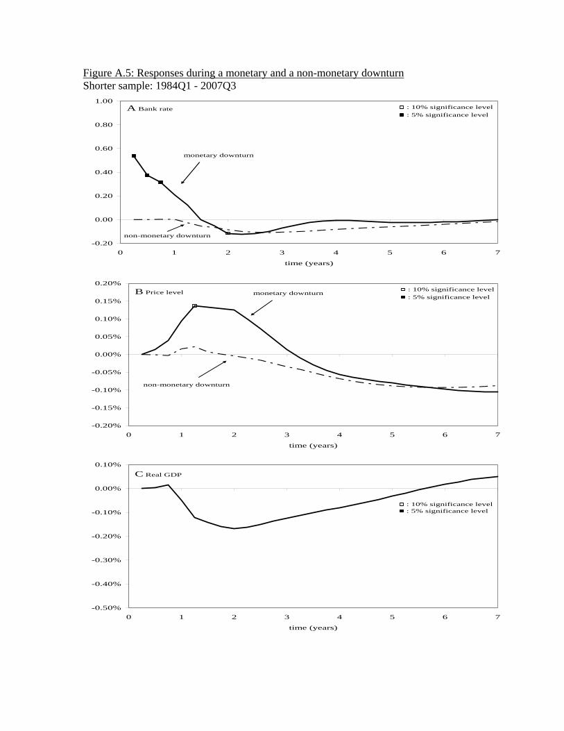
Figure A.5: Responses during a monetary and a non-monetary downturn Shorter sample: 1984Q1 - 2007Q3

-0.20

0.00

0.20

0.40

0.60

0.80

1.00

0 1 2 3 4 5 6 7

time (years)


monetary downturn


A Bank rate

-0.20%

-0.15%

-0.10%

-0.05%

0.00%

0.05%

0.10%

0.15%

0.20%

0 1 2 3 4 5 6 7

time (years)


monetary downturn


B Price level

-0.50%

-0.40%

-0.30%

-0.20%

-0.10%

0.00%

0.10%

0 1 2 3 4 5 6 7

time (years)


C Real GDP

-0.50%

-0.40%

-0.30%

-0.20%

-0.10%

0.00%

0.10%

0.20%

0.30%

0.40%

0.50%

0 1 2 3 4 5 6 7

time (years)


monetary downturn



-1.00%

-0.80%

-0.60%

-0.40%

-0.20%

0.00%

0.20%

0 1 2 3 4 5 6 7

time (years)


monetary downturn



-0.50%

-0.40%

-0.30%

-0.20%

-0.10%

0.00%

0.10%

0.20%

0.30%

0.40%

0.50%

0 1 2 3 4 5 6 7

time (years)


monetary downturn



-1.00%

-0.80%

-0.60%

-0.40%

-0.20%

0.00%

0.20%

0.40%

0.60%

0.80%

1.00%

0 1 2 3 4 5 6 7

time (years)


monetary downturn




Figure A6: Responses during a monetary and a non-monetary downturn Inventories are added to VAR and to the definition of a non-monetary downturn

-2.00%

-1.50%

-1.00%

-0.50%

0.00%

0.50%

1.00%

1.50%

0 1 2 3 4 5 6 7

time (years)


monetary downturn


Non-mortgage business

Note: The graph plot the responses of non-mortgage business loans to a one-standard-deviation monetary policy shock (monetary downturn) and the responses to a sequence of output shocks and inventory shocks that result in the same response for real output and inventories (non-monetary downturn).

bank loan portfolios and the canadian ... - wouter den … loan portfolios and the canadian monetary...

Documents