vector autoregressions (vars) - wouter den haan · vector autoregressions (vars) wouter j. den haan...
TRANSCRIPT
Vector Autoregressions (VARs)
Wouter J. Den HaanLondon School of Economics
Wouter J. Den Haan
March 23, 2018

Intro & IRFs Reduced-form VARs Estimation Structural VARs Critiques
Overview
• Impulse Response Functions• Reduced form & Structural VARs
• Short-term restrictions• Long-term restrictions• Sign restrictions
• Estimation• Problems/topics

Intro & IRFs Reduced-form VARs Estimation Structural VARs Critiques
How to estimate/evaluate models?
• Full information methods like ML and its Bayesian version takeevery aspect of the model as truth
• A less ambitious approach is to focus on just some "keyproperties"
• both in the model and in the data
• What properties?• means, standard deviations, cross-correlations• but propagation of shocks is key aspect of economic models=⇒ autocovariance say something about this but not in themost intuitive way
• IRFs are better for this

Intro & IRFs Reduced-form VARs Estimation Structural VARs Critiques
General definition IRFs
• Suppose
yt = f (yt−1, yt−2, · · · , yt−p, εt) and εt has a variance equal to σ2
• The IRF gives the jth-period response when the system isshocked by a one-standard-deviation shock.
Intro & IRFs Reduced-form VARs Estimation Structural VARs Critiques
General definition IRFs
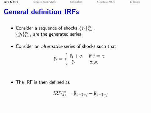
• Consider a sequence of shocks {εt}∞t=1.
{yt}∞t=1 are the generated series
• Consider an alternative series of shocks such that
εt =
{εt + σ if t = τεt o.w.
• The IRF is then defined as
IRF(j) = yτ−1+j − yτ−1+j

Intro & IRFs Reduced-form VARs Estimation Structural VARs Critiques
IRFs for linear processes
• Linear processes: The IRF is independent of the particulardraws for εt
• Thus we can simply start at the steady state (that is when εthas been zero for a very long time)
• The effect of a shock of size Λσ is Λ times the effect of ashock of size σ
Intro & IRFs Reduced-form VARs Estimation Structural VARs Critiques
IRFs for linear processes
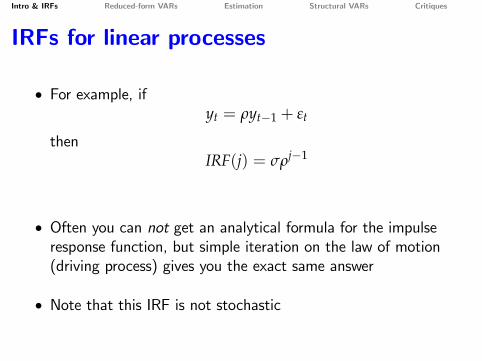
• For example, ifyt = ρyt−1 + εt
thenIRF(j) = σρj−1
• Often you can not get an analytical formula for the impulseresponse function, but simple iteration on the law of motion(driving process) gives you the exact same answer
• Note that this IRF is not stochastic
Intro & IRFs Reduced-form VARs Estimation Structural VARs Critiques
IRFs for nonlinear processes
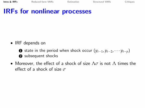
• IRF depends on1 state in the period when shock occur (yt−1, yt−2, · · · yt−p)2 subsequent shocks
• Moreover, the effect of a shock of size Λσ is not Λ times theeffect of a shock of size σ
Intro & IRFs Reduced-form VARs Estimation Structural VARs Critiques
IRFs in theoretical models
• When you have solved for the policy functions, then it is trivialto get the IRFs by simply giving the system a one standarddeviation shock and iterating on the policy functions.
• Shocks in the model are structural shocks, such as• productivity shock• preference shock• monetary policy shock

Intro & IRFs Reduced-form VARs Estimation Structural VARs Critiques
IRFs in the data
The big question
• Can we estimate IRFs from the data without specifying anexplicit theoretical model
• That is what structural VARs attempt to do

Intro & IRFs Reduced-form VARs Estimation Structural VARs Critiques
VARs & IRFs
What we are going to do?
• Describe an empirical model that has turned out to be veryuseful (for example for forecasting)
• Reduced-form VAR
• Describe a way to back out structural shocks (this is the hardpart)
• Structural-VAR
Intro & IRFs Reduced-form VARs Estimation Structural VARs Critiques
Reduced Form VARs
• Let yt be an n× 1 vector of n variables (typically in logs)
yt =J
∑j=1
Ajyt−j + ut
where Aj is an n× n matrix.
• Wold representation is a justification for the linearity.
Intro & IRFs Reduced-form VARs Estimation Structural VARs Critiques
Reduced Form Vector AutoRegressivemodels (VARs)
• constants and trend terms are left out to simplify the notation
• This system can be estimated by OLS (equation by equation)even if yt contains I(1) variables
Intro & IRFs Reduced-form VARs Estimation Structural VARs Critiques
Estimation of VARs
yt =J
∑j=1
Ajyt−j + ut
Claim:
• You can simply estimate a VAR in (log) levels even if variablesare I(1) (and even when you have higher-order integration aslong as you have enough lags)
• Why?

Intro & IRFs Reduced-form VARs Estimation Structural VARs Critiques
Spurious regression
• Let zt and xt be I(1) variables that have nothing to do witheach other
• Consider the regression equation
zt = axt + ut
• The least-squares estimator is given by
aT =∑T
t=1 xtzt
∑Tt=1 x2
t
• Problem:lim
T−→∞aT 6= 0
Intro & IRFs Reduced-form VARs Estimation Structural VARs Critiques
Source of spurious regressions
• The problem is not that zt and xt are I(1)• The problem is that there is not a single value for a such that
ut is stationary• If zt and xt are cointegrated then there is a value of a such that
zt − axt is stationary
• Then least-squares estimates of a are consistent• but you have to change formula for standard errors
Intro & IRFs Reduced-form VARs Estimation Structural VARs Critiques
How to avoid spurious regressions?
Answer: Add enough lags.
• Consider the following regression equation
zt = axt + bzt−1 + ut
• Now there are values of the regression coeffi cients so that ut isstationary, namely
a = 0 and b = 1
• So as long as you have enough lags in the VAR you are fine(but be careful with inferences)
Intro & IRFs Reduced-form VARs Estimation Structural VARs Critiques
How to get standard errors?
• If all data series are stationary you can get standard errors usingthe usual formulas (see Hamilton 1994).
• If they are not you can use bootstrapping
Intro & IRFs Reduced-form VARs Estimation Structural VARs Critiques
Bootstrapping
• Supposeyt = ayt−1 + εt
aT =∑ ytyt−1
∑ yt−1yt−1
• How to get standard errors for IRF?technique easily generates for more complex VAR and otherstatistics

Intro & IRFs Reduced-form VARs Estimation Structural VARs Critiques
Bootstrapping
1. Estimate model and IRF
2. Calculate residuals, {εt}Tt=2 = Θ
3. Generate J new sample of length T from
zt = aTzt−1 + et
z1 = y1
et is drawn from Θ
Intro & IRFs Reduced-form VARs Estimation Structural VARs Critiques
Bootstrapping
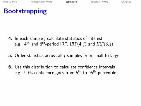
4. In each sample j calculate statistics of interest,e.g., 4th and 6th-period IRF, IRF(4, j) and IRF(6, j)
5. Order statistics across all J samples from small to large
6. Use this distribution to calculate confidence intervalse.g., 90% confidence goes from 5th to 95th percentile
Intro & IRFs Reduced-form VARs Estimation Structural VARs Critiques
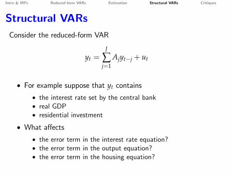
Structural VARsConsider the reduced-form VAR
yt =J
∑j=1
Ajyt−j + ut
• For example suppose that yt contains
• the interest rate set by the central bank• real GDP• residential investment
• What affects• the error term in the interest rate equation?• the error term in the output equation?• the error term in the housing equation?

Intro & IRFs Reduced-form VARs Estimation Structural VARs Critiques
Structural shocks
• Suppose that the economy is being hit by "structural shocks",that is shocks that are not responses to economic events
• Suppose that there are 10 structural shocks. Thus
ut = Bet
where B is a 3× 10 matrix.• Without loss of generality we can assume that
E[ete′t] = I

Intro & IRFs Reduced-form VARs Estimation Structural VARs Critiques
Structural shocks
• Can we identify B from the data?
E[utu′t] = BE[ete′t]B′ = BB′
• We can get an estimate for E[utu′t] using
Σ =T
∑t=J+1
utu′t/(T− J)
• But B contains 30 unknowns and
E[utu′t
]= BB′
has only 9 equations
Intro & IRFs Reduced-form VARs Estimation Structural VARs Critiques
Identification of B
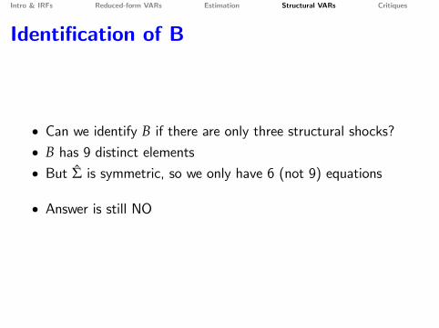
• Can we identify B if there are only three structural shocks?• B has 9 distinct elements• But Σ is symmetric, so we only have 6 (not 9) equations
• Answer is still NO
Intro & IRFs Reduced-form VARs Estimation Structural VARs Critiques
Identification of B
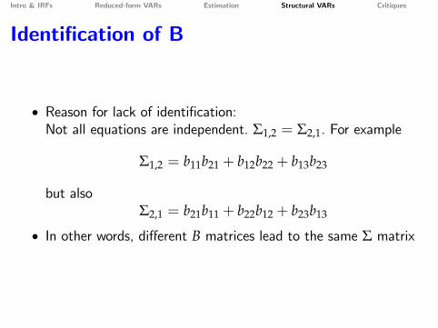
• Reason for lack of identification:Not all equations are independent. Σ1,2 = Σ2,1. For example
Σ1,2 = b11b21 + b12b22 + b13b23
but alsoΣ2,1 = b21b11 + b22b12 + b23b13
• In other words, different B matrices lead to the same Σ matrix
Intro & IRFs Reduced-form VARs Estimation Structural VARs Critiques
Identification of B
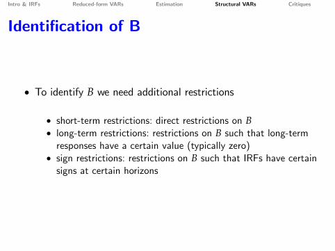
• To identify B we need additional restrictions
• short-term restrictions: direct restrictions on B• long-term restrictions: restrictions on B such that long-termresponses have a certain value (typically zero)
• sign restrictions: restrictions on B such that IRFs have certainsigns at certain horizons

Intro & IRFs Reduced-form VARs Estimation Structural VARs Critiques
Identification of B
uit
uyt
urt
= B
e1t
e2t
empt
• Suppose we impose
B =
0 00
• Then I can solve for the remaining elements of B from
BB′ = Σ
Intro & IRFs Reduced-form VARs Estimation Structural VARs Critiques
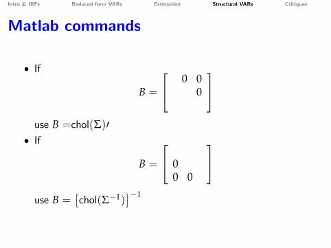
Matlab commands
• If
B =
0 00
use B =chol(Σ)′
• If
B =
00 0
use B =
[chol(Σ−1)
]−1
Intro & IRFs Reduced-form VARs Estimation Structural VARs Critiques
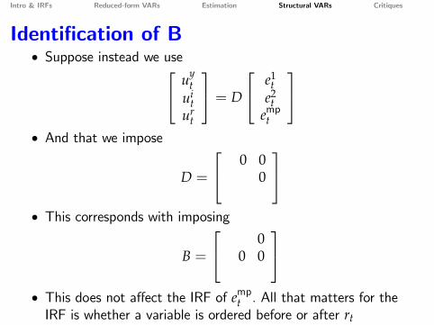
Identification of B• Suppose instead we use uy
tui
tur
t
= D
e1t
e2t
empt
• And that we impose
D =
0 00
• This corresponds with imposing
B =
00 0
• This does not affect the IRF of empt . All that matters for theIRF is whether a variable is ordered before or after rt

Intro & IRFs Reduced-form VARs Estimation Structural VARs Critiques
Calculating IRFs from (structural) VAR
1 Calculation IRFs from first-order VAR is trivial
2 Calculation IRFs from higher-order VAR is also trivial,since higher-order VARs can be written as first-order system(or you simply iterate on the system)
Intro & IRFs Reduced-form VARs Estimation Structural VARs Critiques
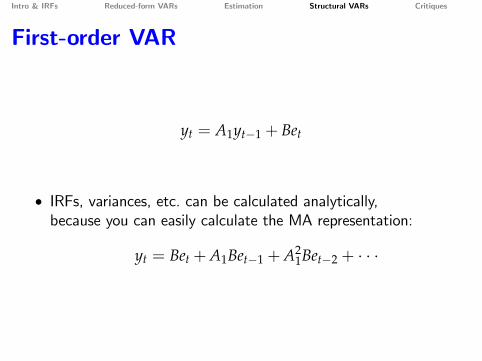
First-order VAR
yt = A1yt−1 + Bet
• IRFs, variances, etc. can be calculated analytically,because you can easily calculate the MA representation:
yt = Bet +A1Bet−1 +A21Bet−2 + · · ·
Intro & IRFs Reduced-form VARs Estimation Structural VARs Critiques
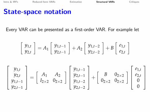
State-space notation
Every VAR can be presented as a first-order VAR. For example let
[y1,ty2,t
]= A1
[y1,t−1y2,t−1
]+A2
[y1,t−2y2,t−2
]+ B
[e1,te2,t
]
y1,ty2,t
y1,t−1y2,t−1
= [ A1 A2I2×2 02×2
] y1,t−1y2,t−1y1,t−2y2,t−2
+ [ B 02×202×2 02×2
] e1,te2,t00
Intro & IRFs Reduced-form VARs Estimation Structural VARs Critiques
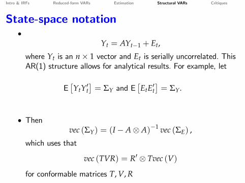
State-space notation•
Yt = AYt−1 + Et,
where Yt is an n× 1 vector and Et is serially uncorrelated. ThisAR(1) structure allows for analytical results. For example, let
E[YtY′t
]= ΣY and E
[EtE′t
]= ΣY.
• Thenvec (ΣY) = (I−A⊗A)−1 vec (ΣE) ,
which uses that
vec (TVR) = R′ ⊗ Tvec (V)
for conformable matrices T, V, R
Intro & IRFs Reduced-form VARs Estimation Structural VARs Critiques
Alternative identification assumptions
• restrictions do not have to be zero restrictions
• you can impose restrictions on B such that IRFs have certainpropertiesthen restrictions imposed depend on rest of the VAR

Intro & IRFs Reduced-form VARs Estimation Structural VARs Critiques
Identifying assumption (Blanchard-Quah)
VAR used by Gali (1999)
zt =J
∑j=1
Ajzt−j + Bεt
with
zt =
[∆ ln(yt/ht)
∆ ln(ht)
]εt =
[εt,technology
εt,non-technology
]
Intro & IRFs Reduced-form VARs Estimation Structural VARs Critiques
Identifying assumption (Blanchard-Quah)
• Non-technology shock does not have a long-run impact onproductivity
• Long-run impact is zero if• Response of the level goes to zero• Responses of the differences sum to zero

Intro & IRFs Reduced-form VARs Estimation Structural VARs Critiques
Get MA representation
zt = A(L)zt + Bεt
= (I−A(L))−1Bεt
= D(L)εt
= D0εt +D1εt−1 + · · ·
Note that D0 = B
Intro & IRFs Reduced-form VARs Estimation Structural VARs Critiques
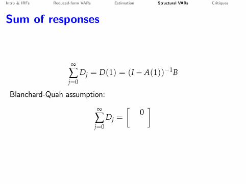
Sum of responses
∞
∑j=0
Dj = D(1) = (I−A(1))−1B
Blanchard-Quah assumption:
∞
∑j=0
Dj =
[0]
Intro & IRFs Reduced-form VARs Estimation Structural VARs Critiques
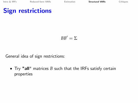
Sign restrictions
BB′ = Σ
General idea of sign restrictions:
• Try "all" matrices B such that the IRFs satisfy certainproperties

Intro & IRFs Reduced-form VARs Estimation Structural VARs Critiques
Sign restrictions - example• Try "all" matrices B such that the IRFs satisfy certainproperties such as• In response to an expansionary monetary policy shock, theinterest rate falls while money and prices rise.
• In response to a positive shock to money demand, both theinterest rate and money increase.
• In response to a positive demand shock, both output andprices rise.
• In response to a positive supply shock, output rises but pricesfall.
• In response to a positive external shock, the exchange ratedevaluates and output increases.
• You would have to specify the horizon for which this should hold
These examples are from Rubio-Ramirez, Waggoner, Zha (2005).
Intro & IRFs Reduced-form VARs Estimation Structural VARs Critiques
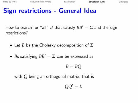
Sign restrictions - General Idea
How to search for "all" B that satisfy BB′ = Σ and the signrestrictions?
• Let B be the Cholesky decomposition of Σ
• Bs satisfying BB′ = Σ can be expressed as
B = BQ
with Q being an orthogonal matrix, that is
QQ′ = I.

Intro & IRFs Reduced-form VARs Estimation Structural VARs Critiques
Sign restrictions - In practice
"Systematically" look for Q such that
1
QQ′ = I.
2
B = QB satisfies the sign restricions
Intro & IRFs Reduced-form VARs Estimation Structural VARs Critiques
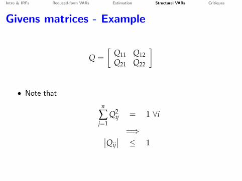
Givens matrices - Example
Q =
[Q11 Q12Q21 Q22
]
• Note thatn
∑j=1
Q2ij = 1 ∀i
=⇒∣∣Qij∣∣ ≤ 1

Intro & IRFs Reduced-form VARs Estimation Structural VARs Critiques
Sign restrictions - Givens matrices
• Suppose that B is a 2× 2 Matrix
• Then all Qs satisfying QQ′ = I can be represented with thefollowing Givens matrices
rotation : Qrot =
[cos θ − sin θsin θ cos θ
],−π ≤ θ ≤ π
reflection : Qref =
[− cos θ sin θ
sin θ cos θ
],−π ≤ θ ≤ π
• In practice you can use a grid for θ or draw θ from a uniformdistribution

Intro & IRFs Reduced-form VARs Estimation Structural VARs Critiques
Number of Givens matrices• Let’s index Q by the Q21 element, that is,
Q21 = ω with − 1 ≤ ω ≤ 1
• For each ω there are (at most) four different solutions forQ11, Q12, and Q22
Q211 +Q2
12 = 1Q11ω+Q12Q22 = 0
ω+Q222 = 1
• Thus, focusing on QQ′ = I equation indicates there are 4 Qsfor every ω.
• ω = sin θ has two solutions for θ =⇒ again 4 Qs (two Qrotsand two Qrefs).

Intro & IRFs Reduced-form VARs Estimation Structural VARs Critiques
Givens matrices - Third Order
Qrot1 = cos θ1 − sin θ1 0
sin θ1 cos θ1 00 0 1
Qrot
2 = cos θ2 0 − sin θ20 1 0
sin θ2 0 cos θ2
Qrot
3 1 0 00 cos θ3 − sin θ30 sin θ3 cos θ3

Intro & IRFs Reduced-form VARs Estimation Structural VARs Critiques
Givens matrices - Third Order
Qref1 = − cos θ1 sin θ1 0
sin θ1 cos θ1 00 0 1
Qref
2 = − cos θ2 0 sin θ20 1 0
sin θ2 0 cos θ2
Qref
3 = 1 0 00 − cos θ3 sin θ30 sin θ3 cos θ3

Intro & IRFs Reduced-form VARs Estimation Structural VARs Critiques
Givens matrices - Third Order
For each combination of θ1, θ2, and θ3 consider
Q =3
∏i=1
Qri (θi) for r ∈ {rot,ref}
Intro & IRFs Reduced-form VARs Estimation Structural VARs Critiques
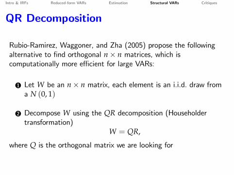
QR Decomposition
Rubio-Ramirez, Waggoner, and Zha (2005) propose the followingalternative to find orthogonal n× n matrices, which iscomputationally more effi cient for large VARs:
1 Let W be an n× n matrix, each element is an i.i.d. draw froma N (0, 1)
2 Decompose W using the QR decomposition (Householdertransformation)
W = QR,
where Q is the orthogonal matrix we are looking for
Intro & IRFs Reduced-form VARs Estimation Structural VARs Critiques
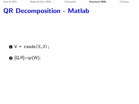
QR Decomposition - Matlab
1 W = randn(3,3);
2 [Q,R]=qr(W);
Intro & IRFs Reduced-form VARs Estimation Structural VARs Critiques
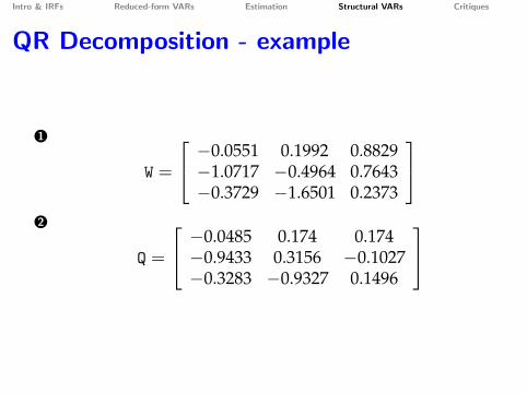
QR Decomposition - example
1
W =
−0.0551 0.1992 0.8829−1.0717 −0.4964 0.7643−0.3729 −1.6501 0.2373
2
Q =
−0.0485 0.174 0.174−0.9433 0.3156 −0.1027−0.3283 −0.9327 0.1496
Intro & IRFs Reduced-form VARs Estimation Structural VARs Critiques
Sign restrictions - comments
• Sign restrictions give you a set of IRFs.If you would plot the median at each horizon then this typicallywould be a combination of different IRFs, that is, there maynot be one IRF that is close to what you are plotting
• When using sign restrictions in a Bayesian framework, then youshould be careful that drawing from the posterior does notimpose additional restrictions (See Arias, Rubio-Ramirez andWaggoner 2014 discuss this and provide a mechanism to dothis right)

Intro & IRFs Reduced-form VARs Estimation Structural VARs Critiques
If you ever feel bad about getting too muchcriticism ....
•
• be glad you are not a structural VAR

Intro & IRFs Reduced-form VARs Estimation Structural VARs Critiques
If you ever feel bad about getting too muchcriticism ....
•• be glad you are not a structural VAR
Intro & IRFs Reduced-form VARs Estimation Structural VARs Critiques
Structural VARs & critiques
• From MA to AR• Lippi & Reichlin (1994)
• From prediction errors to structural shocks• Fernández-Villaverde, Rubio-Ramirez, Sargent, Watson (2007)
• Problems in finite samples• Chari, Kehoe, McGratten (2008)

Intro & IRFs Reduced-form VARs Estimation Structural VARs Critiques
From MA to AR
Consider the two following different MA(1) processes
yt = εt +12
εt−1, Et [εt] = 0, Et
[ε2
t
]= σ2
xt = et + 2et−1, Et [et] = 0, Et
[e2
t
]= σ2/4
• Different IRFs• Same variance and covariance
E[ytyt−j
]= E
[xtxt−j
]
Intro & IRFs Reduced-form VARs Estimation Structural VARs Critiques
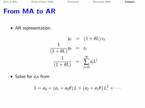
From MA to AR
• AR representation:
yt = (1+ θL) εt1
(1+ θL)yt = εt
1(1+ θL)
=∞
∑j=0
ajLj
• Solve for ajs from
1 = a0 + (a1 + a0θ) L+ (a2 + a1θ) L2 + · · ·
Intro & IRFs Reduced-form VARs Estimation Structural VARs Critiques
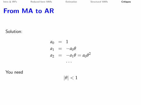
From MA to AR
Solution:
a0 = 1a1 = −a0θ
a2 = −a1θ = a0θ2
· · ·
You need|θ| < 1

Intro & IRFs Reduced-form VARs Estimation Structural VARs Critiques
Prediction errors and structural shocks
Solution to economic model
xt+1 = Axt + Bεt+1
yt+1 = Cxt +Dεt+1
• xt: state variables• yt: observables (used in VAR)• εt: structural shocks
Intro & IRFs Reduced-form VARs Estimation Structural VARs Critiques
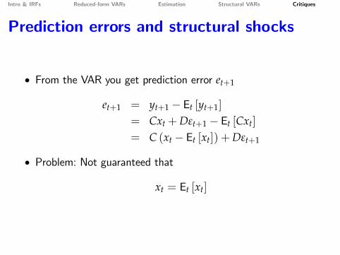
Prediction errors and structural shocks
• From the VAR you get prediction error et+1
et+1 = yt+1 − Et [yt+1]
= Cxt +Dεt+1 − Et [Cxt]
= C (xt − Et [xt]) +Dεt+1
• Problem: Not guaranteed that
xt = Et [xt]
Intro & IRFs Reduced-form VARs Estimation Structural VARs Critiques
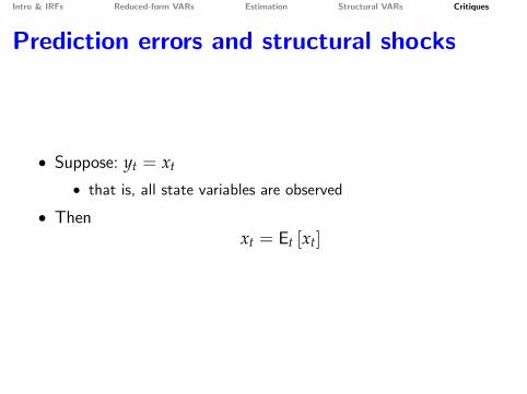
Prediction errors and structural shocks
• Suppose: yt = xt
• that is, all state variables are observed
• Thenxt = Et [xt]
Intro & IRFs Reduced-form VARs Estimation Structural VARs Critiques
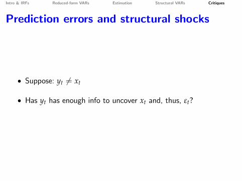
Prediction errors and structural shocks
• Suppose: yt 6= xt
• Has yt has enough info to uncover xt and, thus, εt?
Intro & IRFs Reduced-form VARs Estimation Structural VARs Critiques
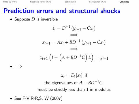
Prediction errors and structural shocks• Suppose D is invertible
εt = D−1 (yt+1 − Cxt)
=⇒xt+1 = Axt + BD−1 (yt+1 − Cxt)
=⇒
xt+1
(I−
(A+ BD−1C
)L)= yt+1
• =⇒
xt = Et [xt] if
the eigenvalues of A− BD−1Cmust be strictly less than 1 in modulus
• See F-V,R-R,S, W (2007)

Intro & IRFs Reduced-form VARs Estimation Structural VARs Critiques
Finite sample problems
• Summary of discussion above• Life is excellent if you observe all state variables• But,
• we don’t observe capital (well)• even harder to observe news about future changes
• If ABCD condition is satisfied, you are still ok in theory
• Problem: you may need ∞-order VAR for observables• recall that kt has complex dynamics

Intro & IRFs Reduced-form VARs Estimation Structural VARs Critiques
Finite sample problems
1 Bias of estimated VAR
• apparently bigger for VAR estimated in first differences
2 Good VAR may need many lags

Intro & IRFs Reduced-form VARs Estimation Structural VARs Critiques
Alleviating finite sample problems
Do with model exactly what you do with data:
• NOT: compare data results with model IRF• YES:
• generate N samples of length T• calculate IRFs as in data• compare average across N samples with data analogue
This is how Kydland & Prescott calculated business cycle stats
Intro & IRFs Reduced-form VARs Estimation Structural VARs Critiques
References• Arias, J.E., J.F. Rubio-Ramirez, D.F. Waggoner, Inference Based on SVARs Identified
with Sign and Zero Restrictions: Theory and Applications, Federal Reserve Board
International Finance Discussion Paper 2014-1100. Available at
• http://www.federalreserve.gov/pubs/ifdp/2014/1100/default.htm.
• Chari, V.V., P.J. Kehoe, E.R. McGrattan, 2008, Are structural VARs with long-run
restrictions useful in developing business cycle theory?, Journal of Monetary Economics,
55, 1337-52.
• Fernandez-Villaverde, J., J.F. Rubio-Ramirez, T.J. Sargent, and M.Watson, 2007, ABCs
(and Ds) of Understanding VARs, Econometrica, 97, 1021-26.
Gives conditions whether a particular VAR can infer structural shocks.
• Fry, R. and A. Pagan, 2011, Sign Restrictions in Structual Vector Autoregressions: A
Critical Review, Journal of Economic Literature, 49, 938-960.
• overview of sign restrictions in VARs and detailed discussion of its weaknesses

Intro & IRFs Reduced-form VARs Estimation Structural VARs Critiques
• Kilian, Lutz, 2011, Structural Vector Autogressions.
• Overview paper that gives several examples of identification choices for different
theoretical models. Available at
• http://www-personal.umich.edu/~lkilian/elgarhdbk_kilian.pdf.
• Lippi, M., and L. Reichlin, 1994, VAR analysis, nonfundamental representations,
Blaschke matrices, Journal of Econometrics, 63, 307-325.
• Luetkepohl, H., 2011, Vector Autoregressive Models, EUI Working Papers
ECO2011/30.
• detailed paper on estimating and working with VARs. Available at
• cadmus.eui.eu/bitstream/handle/1814/19354/ECO_2011_30.pdf

Intro & IRFs Reduced-form VARs Estimation Structural VARs Critiques
• Rubio-Ramirez, Juan F., D.F. Waggoner, and T. Zha, 2005, Markov-Switching
Structural Vector Autogressions: Theory and Applications, Federal Reserve Bank of
Atlanta Working Paper 2005-27.
• contains a detailed discussion of different identification schemes and sign
restrictions in particular. Available at
• http://www.frbatlanta.org/filelegacydocs/wp0527.pdf.
• Whelan, K.,2014 MA Advanced Macroeconomics.
• Set of slides with more detailed info and a discussion of several empirical
examples. Available at
• http://www.karlwhelan.com/MAMacro/part2.pdf
• http://www.karlwhelan.com/MAMacro/part3.pdf
• http://www.karlwhelan.com/MAMacro/part4.pdf