Louisiana Barrier Island Comprehensive Monitoring Program (BICM)  Volume 3: Bathymetry and Historical Seafloor Change 1869‐2007 Part 1: South‐Central Louisiana and Northern Chandeleur Islands, 

Bathymetry Methods and Uncertainty Analysis  

  

Final Report January 2009 

  

 Michael Miner, Mark Kulp, Shea Penland, Dallon Weathers, Jeffrey P. Motti, Phil McCarty, Michael 

Brown, Luis Martinez, and Julie Torres University of New Orleans, Pontchartrain Institute for Environmental Sciences,  

2000 Lakeshore Dr., New Orleans, LA 70148   

James G. Flocks, Nancy Dewitt, Nick Ferina, and B.J. Reynolds U.S. Geological Survey Florida Integrated Science Center,  

600 4th St. South, St. Petersburg, FL 33701  

Dave Twichell, Wayne Baldwin, Bill Danforth, Chuck Worley, and Emile Bergeron U.S. Geological Survey, Woods Hole Science Center,  

384 Woods Hole Road, Quissett Campus, Woods Hole, MA 02543‐1598 

 Louisiana Barrier Island Comprehensive Monitoring Program (BICM) Volume 3: Bathymetry and Historical Seafloor Change 1869-2007 Part 1: Methods and Error Analysis for Bathymetry Final Report January 2009 Michael Miner, Mark Kulp, Shea, Penland, Dallon Weathers, Jeffrey P. Motti, Phil McCarty, Michael Brown, Luis Martinez, and Julie Torres University of New Orleans, Pontchartrain Institute for Environmental Sciences, 2000 Lakeshore Dr., New Orleans, LA, 70148 James Flocks, Nancy Dewitt, Nick Ferina, and B.J. Reynolds U.S. Geological Survey, Florida Integrated Science Center, 600 4th St. South, St. Petersburg, FL 33701 David Twichell, Wayne Baldwin, Bill Danforth, Chuck Worley, and Emile Bergeron U.S. Geological Survey, Woods Hole Science Center, 384 Woods Hole Road, Quissett Campus, Woods Hole, MA, 02543-1598

Funding for this project was provided by the LCA Science & Technology Program, a partnership between the Louisiana Department of Natural Resources (LDNR) and the U.S. Army Corps of Engineers, through LDNR Interagency Agreement No. 2512-06-06.

ii

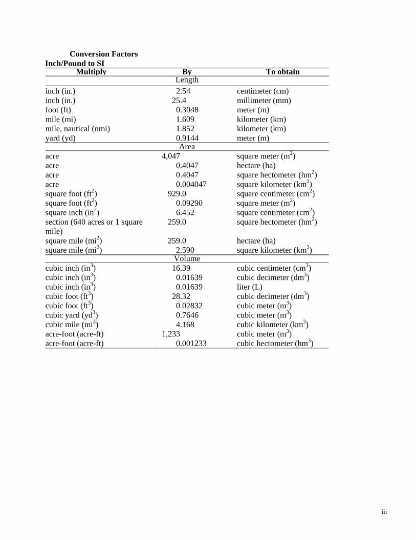
Conversion Factors Inch/Pound to SI

Multiply By To obtain Length

inch (in.) 2.54 centimeter (cm) inch (in.) 25.4 millimeter (mm) foot (ft) 0.3048 meter (m) mile (mi) 1.609 kilometer (km) mile, nautical (nmi) 1.852 kilometer (km) yard (yd) 0.9144 meter (m)

Areaacre 4,047 square meter (m2) acre 0.4047 hectare (ha) acre 0.4047 square hectometer (hm2) acre 0.004047 square kilometer (km2) square foot (ft2) 929.0 square centimeter (cm2) square foot (ft2) 0.09290 square meter (m2) square inch (in2) 6.452 square centimeter (cm2) section (640 acres or 1 square mile)

259.0 square hectometer (hm2)

square mile (mi2) 259.0 hectare (ha) square mile (mi2) 2.590 square kilometer (km2)

Volumecubic inch (in3) 16.39 cubic centimeter (cm3) cubic inch (in3) 0.01639 cubic decimeter (dm3) cubic inch (in3) 0.01639 liter (L) cubic foot (ft3) 28.32 cubic decimeter (dm3) cubic foot (ft3) 0.02832 cubic meter (m3) cubic yard (yd3) 0.7646 cubic meter (m3) cubic mile (mi3) 4.168 cubic kilometer (km3) acre-foot (acre-ft) 1,233 cubic meter (m3) acre-foot (acre-ft) 0.001233 cubic hectometer (hm3)

iii

iv

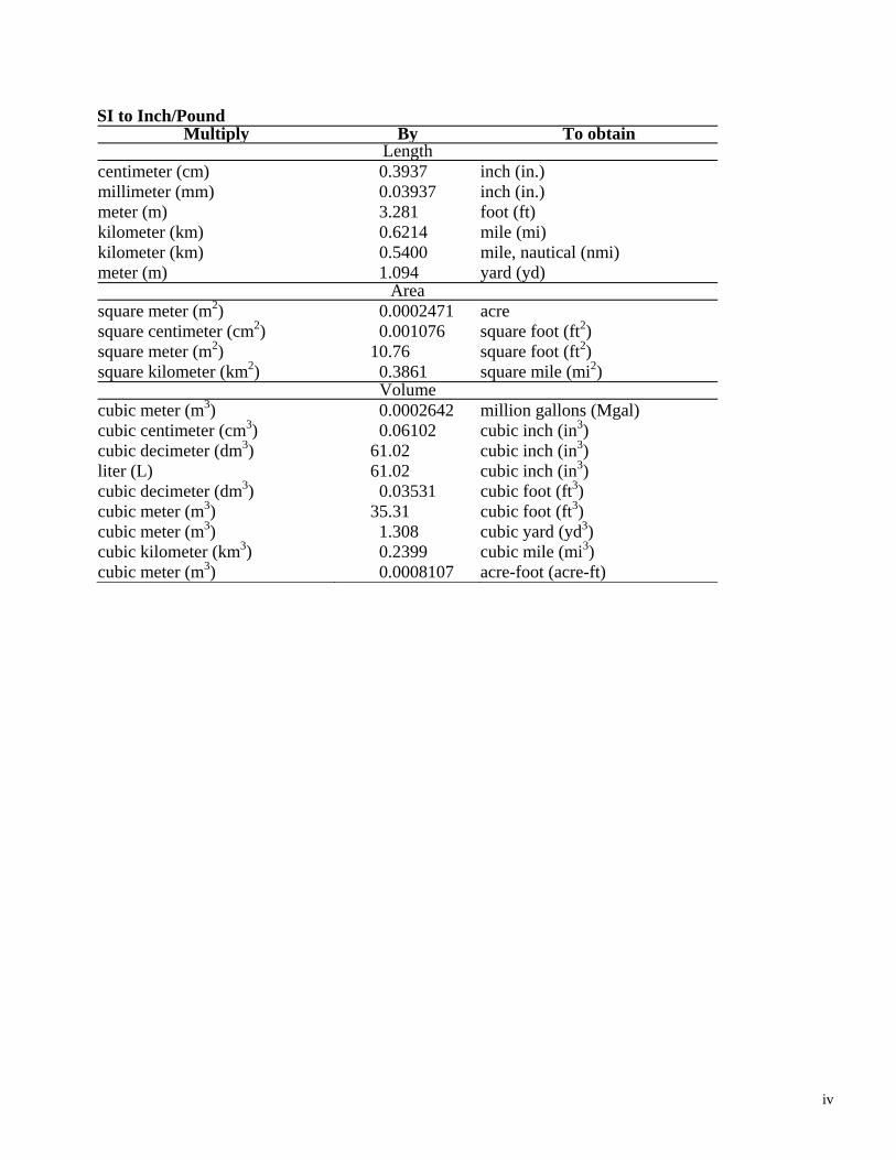
SI to Inch/Pound Multiply By To obtain

Lengthcentimeter (cm) 0.3937 inch (in.) millimeter (mm) 0.03937 inch (in.) meter (m) 3.281 foot (ft) kilometer (km) 0.6214 mile (mi) kilometer (km) 0.5400 mile, nautical (nmi) meter (m) 1.094 yard (yd)

Areasquare meter (m2) 0.0002471 acre square centimeter (cm2) 0.001076 square foot (ft2) square meter (m2) 10.76 square foot (ft2) square kilometer (km2) 0.3861 square mile (mi2)

Volumecubic meter (m3) 0.0002642 million gallons (Mgal) cubic centimeter (cm3) 0.06102 cubic inch (in3) cubic decimeter (dm3) 61.02 cubic inch (in3) liter (L) 61.02 cubic inch (in3) cubic decimeter (dm3) 0.03531 cubic foot (ft3) cubic meter (m3) 35.31 cubic foot (ft3) cubic meter (m3) 1.308 cubic yard (yd3) cubic kilometer (km3) 0.2399 cubic mile (mi3) cubic meter (m3) 0.0008107 acre-foot (acre-ft)

INTRODUCTION

It is widely recognized and well documented that barrier islands and deltaic headland

shorelines of the Louisiana Coastal Zone are rapidly retreating landward and degrading (e.g.

LCA, 2004). High rates of delta plain subsidence, ongoing eustatic sea-level rise, and processes

such as storm impacts collectively contribute to this shoreline loss as shoreline sediment is

eroded or becomes inundated by marine waters (Penland and Ramsey, 1990). The amount of

shoreline retreat along coastal Louisiana has been shown to be as much as 23 m/yr locally

(Williams et al., 1992), and has been a contributing factor to the more than 100 km2 of annual

land loss that has been documented for some select historic time frames across the region (Barras

et al., 2003).

PURPOSE

To more effectively identify the magnitude, rates, and processes of shoreline change a

Barrier Island Comprehensive Monitoring program (BICM) has been developed as a framework

for a coast-wide monitoring effort. A significant component of this effort includes documenting

the historically dynamic morphology of the Louisiana nearshore, shoreline, and backshore zones.

This aspect of the program is designed to complement other more area-specific monitoring

programs that are currently underway through the support of agencies such as the Louisiana

Department of Natural Resources and U.S. Army Corp of Engineers.

The advantage of BICM over current project-specific monitoring efforts is that it will

provide long-term morphological datasets on all of Louisiana's barrier islands and shorelines;

rather than just those islands and areas that are slated for coastal engineering projects or have had

construction previously completed. BICM additionally specifically provides a larger proportion

of unified, long-term datasets that will be available to monitor constructed projects, plan and

design future barrier island projects, develop operation and maintenance activities, and assess the

range of impacts created by past and future tropical storms. The development of coastal models,

such as those quantifying littoral sediment budgets, and a more advanced knowledge of

mechanisms forcing coastal evolution becomes increasingly more regionally feasible with the

availability of BICM datasets. These factors constitute critically important elements of any

effort that is aimed at effective coastal restoration, sediment nourishment, or management.

1

CURRENT BICM GOALS AND TASKS

Data for BICM tasks will be collected and compiled for all of the barrier island systems

and shorelines with similar approaches and methodologies. The resulting data will be more

comparable, consistent, accurate, and complete than currently available barrier island

geomorphology datasets that have been piece-meal constructed and are generally area specific.

In order to achieve the goals of BICM and develop a range of usable, stand-alone datasets the

entire effort has been broken into several research and analysis tasks. These currently include: 1)

the compilation of videography and photography of the 2005 hurricane impacts, 2) the

construction of a unified historic shoreline change database for the Louisiana coastal zone, and

3) the development of a historical bathymetric database with up-to-date 2006 bathymetric

analysis that provides a current seafloor change for the shoreline extending from Sandy Point to

Raccoon Island and the northern Chandeleur Islands, and 4) Light Detection and Ranging

(LiDAR) surveys for the sandy shorelines of the coastal zone. This report describes the

methodologies of constructing a historical bathymetric database, the acquisition and results of

regional 2006 bathymetric survey data, and provides rates of seafloor change derived for a range

of time frames along the Louisiana Coastal Zone study areas (Fig. 1).

PREVIOUS STUDIES

Prior to the implementation of BICM the only available, regionally consistent

documentation for bathymetry and seafloor change was presented in a United States Geological

Survey (USGS) and Louisiana Geological Survey (LGS) atlas on seafloor change (List et al.,

1994). This atlas provided historical bathymetric data from the 1880's, 1930's, and 1980's for the

central Louisiana coastal zone. Patterns and rates of seafloor change (e.g. erosion and deposition)

were identified by an inter-comparison of bathymetry for designated time periods (e.g. 1880’s-

1930’s and 1930's --1980’s) along the south-central Louisiana coastline from Raccoon Island to

Sandy Point. This seminal effort by List et al. (1994) has been invaluable in attempting to

document the regional coastal evolution across multi-decadal time scales. Since the acquisition

of regional data in 1980 and development of the USGS atlas no comparable, comprehensive

effort has been undertaken to document the shallow, nearshore bathymetry and more recent

seafloor change. Moreover, prior to the establishment of the BICM priorities there had been no

single comprehensive database of bathymetry and/or seafloor change for the Chandeleur Islands.

2

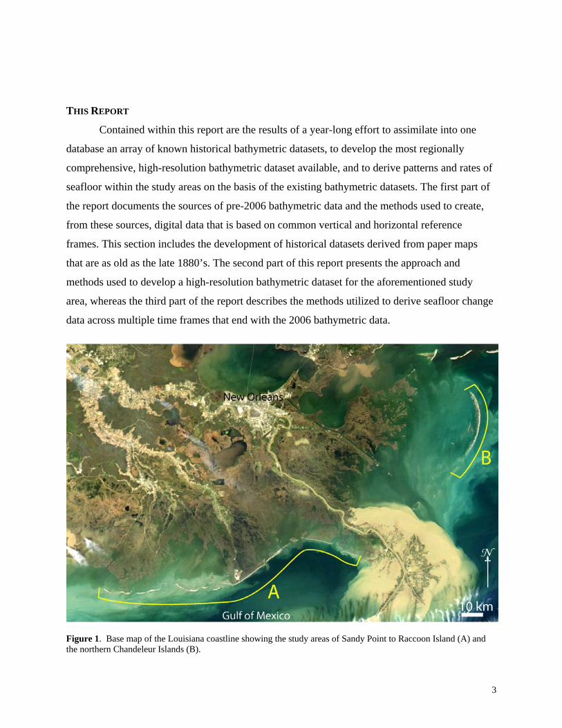
THIS REPORT

Contained within this report are the results of a year-long effort to assimilate into one

database an array of known historical bathymetric datasets, to develop the most regionally

comprehensive, high-resolution bathymetric dataset available, and to derive patterns and rates of

seafloor within the study areas on the basis of the existing bathymetric datasets. The first part of

the report documents the sources of pre-2006 bathymetric data and the methods used to create,

from these sources, digital data that is based on common vertical and horizontal reference

frames. This section includes the development of historical datasets derived from paper maps

that are as old as the late 1880’s. The second part of this report presents the approach and

methods used to develop a high-resolution bathymetric dataset for the aforementioned study

area, whereas the third part of the report describes the methods utilized to derive seafloor change

data across multiple time frames that end with the 2006 bathymetric data.

Figure 1. Base map of the Louisiana coastline showing the study areas of Sandy Point to Raccoon Island (A) and the northern Chandeleur Islands (B).

3

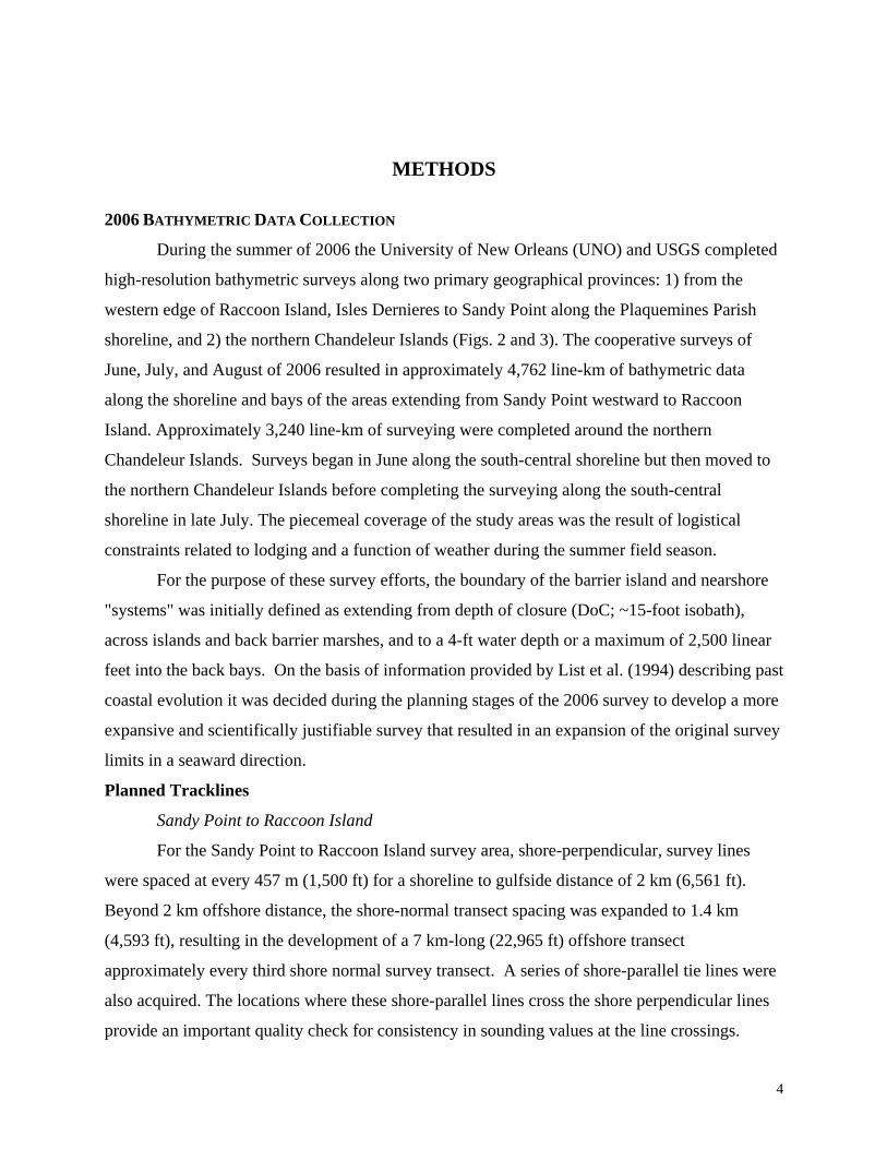
METHODS

2006 BATHYMETRIC DATA COLLECTION

During the summer of 2006 the University of New Orleans (UNO) and USGS completed

high-resolution bathymetric surveys along two primary geographical provinces: 1) from the

western edge of Raccoon Island, Isles Dernieres to Sandy Point along the Plaquemines Parish

shoreline, and 2) the northern Chandeleur Islands (Figs. 2 and 3). The cooperative surveys of

June, July, and August of 2006 resulted in approximately 4,762 line-km of bathymetric data

along the shoreline and bays of the areas extending from Sandy Point westward to Raccoon

Island. Approximately 3,240 line-km of surveying were completed around the northern

Chandeleur Islands. Surveys began in June along the south-central shoreline but then moved to

the northern Chandeleur Islands before completing the surveying along the south-central

shoreline in late July. The piecemeal coverage of the study areas was the result of logistical

constraints related to lodging and a function of weather during the summer field season.

For the purpose of these survey efforts, the boundary of the barrier island and nearshore

"systems" was initially defined as extending from depth of closure (DoC; ~15-foot isobath),

across islands and back barrier marshes, and to a 4-ft water depth or a maximum of 2,500 linear

feet into the back bays. On the basis of information provided by List et al. (1994) describing past

coastal evolution it was decided during the planning stages of the 2006 survey to develop a more

expansive and scientifically justifiable survey that resulted in an expansion of the original survey

limits in a seaward direction.

Planned Tracklines

Sandy Point to Raccoon Island

For the Sandy Point to Raccoon Island survey area, shore-perpendicular, survey lines

were spaced at every 457 m (1,500 ft) for a shoreline to gulfside distance of 2 km (6,561 ft).

Beyond 2 km offshore distance, the shore-normal transect spacing was expanded to 1.4 km

(4,593 ft), resulting in the development of a 7 km-long (22,965 ft) offshore transect

approximately every third shore normal survey transect. A series of shore-parallel tie lines were

also acquired. The locations where these shore-parallel lines cross the shore perpendicular lines

provide an important quality check for consistency in sounding values at the line crossings.

4

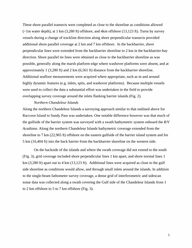
These shore parallel transects were completed as close to the shoreline as conditions allowed

(~1m water depth), at 1 km (3,280 ft) offshore, and 4km offshore (13,123 ft). Turns by survey

vessels during a change of trackline direction along shore perpendicular transects provided

additional shore parallel coverage at 2 km and 7 km offshore. In the backbarrier, shore

perpendicular lines were extended from the backbarrier shoreline to 2 km in the backbarrier-bay

direction. Shore parallel tie lines were obtained as close to the backbarrier shoreline as was

possible, generally along the marsh platform edge where washover platforms were absent, and at

approximately 1 (3,280 ft) and 2 km (6,561 ft) distance from the backbarrier shoreline.

Additional seafloor measurements were acquired where appropriate, such as in and around

highly dynamic features (e.g. inlets, spits, and washover platforms). Because multiple vessels

were used to collect the data a substantial effort was undertaken in the field to provide

overlapping survey coverage around the inlets flanking barrier islands (Fig. 2).

Northern Chandeleur Islands

Along the northern Chandeleur Islands a surveying approach similar to that outlined above for

Raccoon Island to Sandy Pass was undertaken. One notable difference however was that much of

the gulfside of the barrier system was surveyed with a swath bathymetric system onboard the R/V

Acadiana. Along the northern Chandeleur Islands bathymetric coverage extended from the

shoreline to 7 km (22,965 ft) offshore on the eastern gulfside of the barrier island system and for

5 km (16,404 ft) into the back barrier from the backbarrier shoreline on the western side.

On the backside of the islands and where the swath coverage did not extend to the south

(Fig. 3), grid coverage included shore perpendicular lines 1 km apart, and shore normal lines 1

km (3,280 ft) apart out to 4 km (13,123 ft). Additional lines were acquired as close to the gulf

side shoreline as conditions would allow, and through small inlets around the islands. In addition

to the single-beam fathometer survey coverage, a dense grid of interferometric and sidescan

sonar data was collected along a swath covering the Gulf side of the Chandeleur Islands from 1

to 2 km offshore to 5 to 7 km offshore (Fig. 3).

5

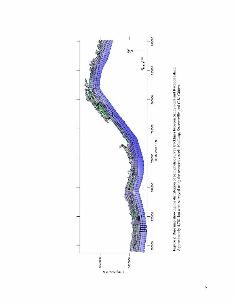
Figu

re 2

. Bas

e m

ap sh

owin

g th

e di

strib

utio

n of

bat

hym

etric

surv

ey tr

ackl

ines

bet

wee

n Sa

ndy

Poin

t and

Rac

coon

Isla

nd.

App

roxi

mat

ely

4,76

2-km

wer

e su

rvey

ed u

sing

the

rese

arch

ves

sels

Mud

lum

p, S

tree

terv

ille,

and

G.K

. Gilb

ert.

6

Figure 3. Base map of the northern Chandeleur Islands with the distribution of bathymetric survey tracklines along the Gulf and Breton Sound side of the barrier island system. The black lines indicate single-beam bathymetry coverage and the red lines indicate swath bathymety coverage. Approximately 3,240-km were surveyed using the research vessels Mudlump, Streeterville, G.K. Gilbert, and Acadiana.

7

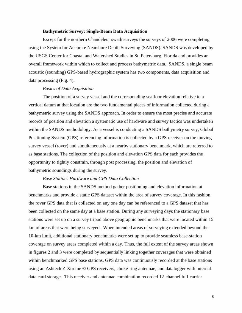
Bathymetric Survey: Single-Beam Data Acquisition

Except for the northern Chandeleur swath surveys the surveys of 2006 were completing

using the System for Accurate Nearshore Depth Surveying (SANDS). SANDS was developed by

the USGS Center for Coastal and Watershed Studies in St. Petersburg, Florida and provides an

overall framework within which to collect and process bathymetric data. SANDS, a single beam

acoustic (sounding) GPS-based hydrographic system has two components, data acquisition and

data processing (Fig. 4).

Basics of Data Acquisition

The position of a survey vessel and the corresponding seafloor elevation relative to a

vertical datum at that location are the two fundamental pieces of information collected during a

bathymetric survey using the SANDS approach. In order to ensure the most precise and accurate

records of position and elevation a systematic use of hardware and survey tactics was undertaken

within the SANDS methodology. As a vessel is conducting a SANDS bathymetry survey, Global

Positioning System (GPS) referencing information is collected by a GPS receiver on the moving

survey vessel (rover) and simultaneously at a nearby stationary benchmark, which are referred to

as base stations. The collection of the position and elevation GPS data for each provides the

opportunity to tightly constrain, through post processing, the position and elevation of

bathymetric soundings during the survey.

Base Station: Hardware and GPS Data Collection

Base stations in the SANDS method gather positioning and elevation information at

benchmarks and provide a static GPS dataset within the area of survey coverage. In this fashion

the rover GPS data that is collected on any one day can be referenced to a GPS dataset that has

been collected on the same day at a base station. During any surveying days the stationary base

stations were set up on a survey tripod above geographic benchmarks that were located within 15

km of areas that were being surveyed. When intended areas of surveying extended beyond the

10-km limit, additional stationary benchmarks were set up to provide seamless base-station

coverage on survey areas completed within a day. Thus, the full extent of the survey areas shown

in figures 2 and 3 were completed by sequentially linking together coverages that were obtained

within benchmarked GPS base stations. GPS data was continuously recorded at the base stations

using an Ashtech Z-Xtreme © GPS receivers, choke-ring antennae, and datalogger with internal

data card storage. This receiver and antennae combination recorded 12-channel full-carrier

8

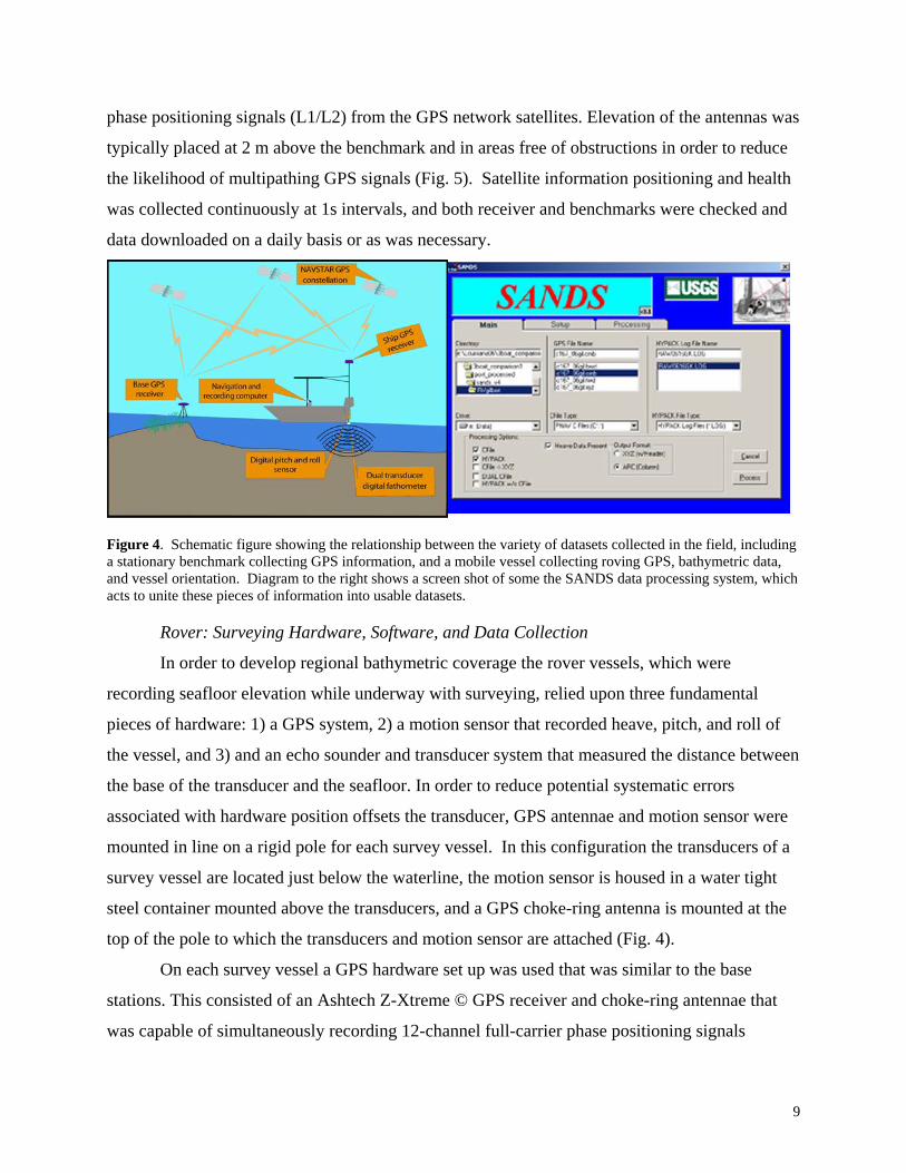
phase positioning signals (L1/L2) from the GPS network satellites. Elevation of the antennas was

typically placed at 2 m above the benchmark and in areas free of obstructions in order to reduce

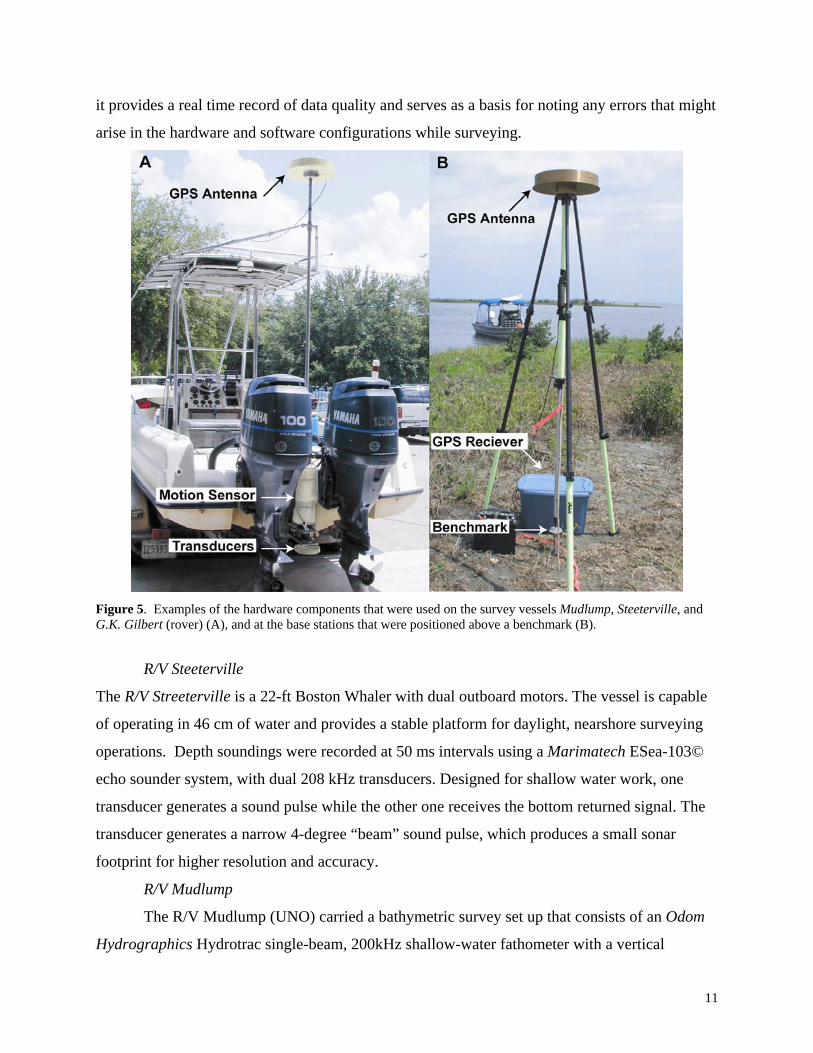
the likelihood of multipathing GPS signals (Fig. 5). Satellite information positioning and health

was collected continuously at 1s intervals, and both receiver and benchmarks were checked and

data downloaded on a daily basis or as was necessary.

Figure 4. Schematic figure showing the relationship between the variety of datasets collected in the field, including a stationary benchmark collecting GPS information, and a mobile vessel collecting roving GPS, bathymetric data, and vessel orientation. Diagram to the right shows a screen shot of some the SANDS data processing system, which acts to unite these pieces of information into usable datasets.

Rover: Surveying Hardware, Software, and Data Collection

In order to develop regional bathymetric coverage the rover vessels, which were

recording seafloor elevation while underway with surveying, relied upon three fundamental

pieces of hardware: 1) a GPS system, 2) a motion sensor that recorded heave, pitch, and roll of

the vessel, and 3) and an echo sounder and transducer system that measured the distance between

the base of the transducer and the seafloor. In order to reduce potential systematic errors

associated with hardware position offsets the transducer, GPS antennae and motion sensor were

mounted in line on a rigid pole for each survey vessel. In this configuration the transducers of a

survey vessel are located just below the waterline, the motion sensor is housed in a water tight

steel container mounted above the transducers, and a GPS choke-ring antenna is mounted at the

top of the pole to which the transducers and motion sensor are attached (Fig. 4).

On each survey vessel a GPS hardware set up was used that was similar to the base

stations. This consisted of an Ashtech Z-Xtreme © GPS receiver and choke-ring antennae that

was capable of simultaneously recording 12-channel full-carrier phase positioning signals

9

(L1/L2) from the NAVSTAR GPS satellites. Similar to the base station recording frequency the

rover receiver recorded position information at 1-second recording intervals throughout

surveying.

Throughout the surveying of both study areas the three primary survey vessels (R/V's

Mudlump, Steeterville, and G.K. Gilbert) were equipped with single beam acquisition systems

(Fig. 5). In general each of these systems consisted of a transducer and fathometer unit that

controlled the rate of pinging from the transducer and processed output and returned transducer

signals into meaningful linear measurements of water depth. The fathometer systems of each

vessel were all set to similar sound velocities (1500 m s-1) and recording rates of soundings (50

ms) but their hardware configurations were different because of the availability of fathometer

systems. The details of each vessels fathometer system are provided in subsequent sections In

addition to the single beam coverage, swath bathymetry data was acquired seaward of the

Chandeleur Islands and a detailed methodology of acquiring these data is also presented in

subsequent sections.

In order to compensate for motion of the rover vessel during surveying all bathymetric

data was real time corrected for heave, pitch, and roll a using a TSS DMS-05 sensor, which

recorded the orientation of the inline GPS antennae and transducer at 50ms intervals. Boat pitch

and roll measurements from the sensor were utilized by SANDS in post-processing of the data.

Heave motion is a major component of potential depth errors and although modern-day motion

sensors can reasonably compensate for vessel motion, they are still subject to constant drifts, and

require visual monitoring (via readout) during survey and in post-processing. In SANDS, the

heave motion from the TSS is not used, but more accurately represented by using the GPS

component.

The data strings from the GPS receiver, motion sensor, and fathometer, were streamed in

real time to an onboard laptop computer running a Windows operating system. The acquisition

software package that was used is HYPACK MAX v4.3A © (HYPACK, INC.), a marine

surveying, positioning, and navigation software package. The acquisition software combines the

data streams from the various components into a single raw data file, with each device string

referenced by a device identification code and timestamp to the nearest millisecond. The

software also manages the planned-transect information, providing real-time navigation, steering,

correction, data quality, and instrumentation-status information to the boat operator. Additionally

10

it provides a real time record of data quality and serves as a basis for noting any errors that might

arise in the hardware and software configurations while surveying.

Figure 5. Examples of the hardware components that were used on the survey vessels Mudlump, Steeterville, and G.K. Gilbert (rover) (A), and at the base stations that were positioned above a benchmark (B).

R/V Steeterville

The R/V Streeterville is a 22-ft Boston Whaler with dual outboard motors. The vessel is capable

of operating in 46 cm of water and provides a stable platform for daylight, nearshore surveying

operations. Depth soundings were recorded at 50 ms intervals using a Marimatech ESea-103©

echo sounder system, with dual 208 kHz transducers. Designed for shallow water work, one

transducer generates a sound pulse while the other one receives the bottom returned signal. The

transducer generates a narrow 4-degree “beam” sound pulse, which produces a small sonar

footprint for higher resolution and accuracy.

R/V Mudlump

The R/V Mudlump (UNO) carried a bathymetric survey set up that consists of an Odom

Hydrographics Hydrotrac single-beam, 200kHz shallow-water fathometer with a vertical

11

resolution of 0.01 meters. The fathometer collected depth soundings at 50 ms intervals through a

side-mounted Odom Hydrographics 200 kHz transducer with a beam width of 3°.

R/V G.K. Gilbert

The G.K. Gilbert is a 50-ft long, shallow draft (3 ft) research vessel that was equipped

with a Knudsen Engineering Limited © 320BP echosounder. The system operated a dual

frequency (28/200 kHz) transducer, pole-mounted midway along the side of the vessel at 1 m

below the water surface. An Ashtech Z-Xtreme GPS receiver system was mounted in-line with

the transducer, and a CodaOctopus F190 motion sensor recorded heave, pitch and roll of the

vessel while surveying.

Bathymetric Survey: Interferometric Swath Data Acquisition

In addition to the single-beam coverage, the USGS conducted a swath bathymetry survey

seaward of the northern Chandeluer Islands. The Louisiana Marine Consortium (LUMCON)

vessel R/V Acadiana surveyed ~ 218 km2 of sea floor using interferometric-sonar, towed

sidescan-sonar, and chirp seismic-reflection geophysical systems. The survey covered a swath ~

45 km long, extending from ~ 1 to 2 km seaward of the shoreline to ~ 5 to 7 km offshore (see

Figure 3). Survey track lines were planned on a dense grid designed to provide 100% coverage

with towed sidescan-sonar data. The towed sidescan sonar system produced a wider swath width

(~ 200 m) than the other systems, which allowed for maximum areal coverage within the allotted

survey period. Shore-parallel lines were spaced ~ 100 m apart inshore of the 6-m depth contour,

and approximately 150-m apart offshore of the 6-m depth contour. Shore-perpendicular lines

were spaced at approximately 1-km along the length of the barrier island system survey.

Bathymetric data were acquired using a SEA Ltd. Submetrix 2000 series interferometric

sonar, that operated at a frequency of 234 kHz. The instrument was mounted on a rigid pole,

along the starboard side of the vessel, at approximately 1.5 m below the sea surface. SEA Ltd.

SwathPlus acquisition software was used to fire the system at a 0.25-s ping rate and digitally log

the data at a 1.5 K sample rate. Vessel motion (heave, pitch, roll, and yaw), which was used to

rectify bathymetric soundings during post-processing, was recorded continuously using a TSS

DMS 2-05 Motion Reference Unit (MRU) mounted directly above the sonar transducers.

Additionally, a Sound Velocity Profiler (SVP) was deployed at ~ 8 hr intervals to record the

sound velocity structure of the water column in the comparatively deeper gulf side survey area.

12

Ship position was recorded the through use of Differential Global Positioning System (DGPS)

navigation. The DGPS antenna was positioned atop the side-mount pole, directly above the sonar

transducers and MRU. The planned track-line spacing resulted in data gaps between adjacent

interferometric-sonar swaths. The width of data gaps varied as a function of track line spacing,

water depth, and avoidance of nautical obstructions. Gap widths ranged from 0 to 60 m inshore

of the 6 m contour, and 20 to 200 m between the 6 m contour and the seaward edge of the

survey.

Swath bathymetric data were rectified for tidal fluctuations using Discrete Tidal Zoning

(DTZ), provided by the National Oceanic and Atmospheric Administration – National Ocean

Service’s Hydrographic Planning Team (Fig. 6; NOAA – NOS HPT,

http://www.tidesandcurrents.noaa.gov/hydro.html). This approach was taken because Real

Time Kinematic – Differential Global Positioning System (RTK – DGPS) height corrections

were not available for the entire survey period. DTZ utilizes a series of GIS polygons (Fig. 6)

that relate offshore tidal characteristics to water level data recorded at one or more tide gauges

within the NOAA – NOS National Water Level Operating Network

(http://www.tidesandcurrents.noaa.gov/station_retrieve.shtml?type=Tide+Data). DTZ time and

height corrections were applied to water level data observed at the Gulfport Harbor, MS tide

station (ID# 8745557) after applying the vertical offset used to reference the station to NAVD88

(NOAA – National Geodetic Survey, http://www.ngs.noaa.gov/cgi-

bin/ngs_opsd.prl?PID=BH0867&EPOCH=1983-2001).

The interferometric-sonar system acquires acoustic backscatter and depth data across a

continuous swath to each side of the survey vessel. Accurate depth solutions are typically

provided across a swath that is 7 to 10 times the water depth. For example, in 3 m water depths

the system could yield a swath width of as much as 30 m (15 m to each side of the vessel).

Within the Chandeleur Islands survey area, swath widths ranged from 20 to 115 m, in 3 to 16 m

depths. Horizontal resolution of the bathymetric data, dictated by DGPS accuracy, was ± 1 – 2

m, and vertical resolution was ~ 1% of water depth, which conforms to the International

Hydrographic Organization (IHO, http://www.iho.shom.fr/) standard requirement of 0.3 m

accuracy in < 30 m water depths.

13

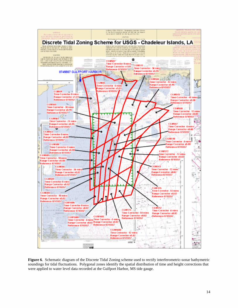
Figure 6. Schematic diagram of the Discrete Tidal Zoning scheme used to rectify interferometric-sonar bathymetric soundings for tidal fluctuations. Polygonal zones identify the spatial distribution of time and height corrections that were applied to water level data recorded at the Gulfport Harbor, MS tide gauge.

14

The linux-based software, SwathEd, developed by the University of New Brunswick –

Ocean Mapping Group (http://www.omg.unb.ca/omg/), was used to post-process the

interferometric-sonar data. Navigation data were inspected and edited, sounding data were

rectified for ship motion, changes in sound velocity within the water column, and DTZ

corrections, and spurious soundings were eliminated. Sounding data were gridded at a 5 m cell

size and exported to an XYZ format that could be used as an input for generation of the

interpolated, area-wide, 100 m cell size bathymetric model.

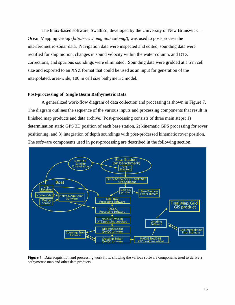
Post-processing of Single Beam Bathymetric Data

A generalized work-flow diagram of data collection and processing is shown in Figure 7.

The diagram outlines the sequence of the various inputs and processing components that result in

finished map products and data archive. Post-processing consists of three main steps: 1)

determination static GPS 3D position of each base station, 2) kinematic GPS processing for rover

positioning, and 3) integration of depth soundings with post-processed kinematic rover position.

The software components used in post-processing are described in the following section.

Figure 7. Data acquisition and processing work flow, showing the various software components used to derive a bathymetric map and other data products.

15

Static Base Station Data Processing

During the survey, static GPS data logged at base stations are submitted to three,

independent GPS autonomous processing software services (OPUS, Auto GYPSY, and SCOUT)

are used to establish position. Through an online submittal service, these automated programs

process the long-duration time-series GPS data recorded by the base station receiver and return a

corrected position relative to constellation conditions on the day of data acquisition.

NOAA and NGS provides the On-Line Positioning User Service (OPUS), which uses

three Continuously Operating Reference Stations (CORS) reference sites to average three

distinct single-baseline solutions computed by double-differenced, carrier phase measurements.

The locations of the three most suitable CORS stations are based upon a series of tests that

OPUS performs to select suitable stations for use in calculations to provide a location accuracy

of 1 to 3 cm.

Automated GPS-Inferred Positioning System (Auto GIPSY), a service provided by

NASA’s Jet Propulsion Laboratory, is applied when the base location cannot be tied to an

established network such as that of the National Geodetic Survey (NGS). Automated GIPSY

software computes base station coordinates by accurately modeling the orbital trajectories of the

NAVSTAR GPS satellites, and provides a base coordinate that can be converted to the NAD 83

and the NAVD 88 datums. Horizontal resolution of the GIPSY output can be less than 1-cm

root-mean square (RMS). The Scripps Coordinate Update Tool (SCOUT) uses the nearest three

International GPS service stations (IGS) to derive a position with similar accuracy to OPUS.

Results from the three processing services are entered into a spreadsheet program for

error analysis and averaging. In order to maintain consistency with LDNR terrestrial surveying

methods and prevent the introduction of errors associated with comparing various statistical

techniques used to derive positions, it was decided that OPUS would be used exclusively for

final base station positions and that SCOUT and GYPSY solutions would be used for validation

only.

The OPUS results are mathematically weighted relative to overall occupation time. The

weighting factor improves accuracy by stressing the significance of longer base station duration

times. Outliers are removed based upon an iterative process of reviewing and eliminating bad

data sessions based on various quality control criteria. The first step is to eliminate any sessions

that have a vertical peak to peak value (OPUS error assessment) greater than 0.04 meters. Next,

16

any sessions having unusually high deviations from the average ellipsoid height are reviewed

and excluded based upon their influence on the mean ellipsoid. The goal is to have all inclusive

sessions to be <0.020 m from the average ellipsoid height. The final 3D position for the base

station is the weighted average of all sessions that were not excluded due to high peak to peak or

deviations from the average ellipsoid height. Final base station positions are included as

Appendix 1 in this report.

Kinematic GPS Processing for Rover Position

Waypoint Inc. GrafNav software is a static/kinematic baseline processing engine

designed to achieve accuracies down to the centimeter level with the ability to incorporate

multiple base station data. In GrafNav output from OPUS are used for kinematic processing of

the rover GPS data to produce a single output of precise boat position and quality control

information at 1-second intervals.

SANDS

An in-house processing program merges the data output (rover kinematic position) from

the GRAFNAV program with the bathymetric data from the Hypack output and performs

geometric corrections of the depth values caused by boat motion, time, and antennae to

transducer offsets. The corrected depth is calculated as follows:

D = ½(v * t) + k + dS + dRP(roll,pitch) + dGPS

Where: v= average velocity of sound in water column t = measured elapsed time from transducer to bottom and back to transducer k = system index constant (constant fathometer bias) dS = offset from transducer face to GPS antenna center dRP = geometric correction applied due to boat roll/pitch motion dGPS = GPS ellipsoid height relative to the GPS antenna center The final output from SANDS produces a 3D position for each sounding referenced vertically to

NAVD88 2004.65 using the NGS GEOID03 revised 10/2005 version for south Louisiana and

horizontally to NAD83 2007 in UTM Zone 15.

Quality control of Single-Beam Data

Sound velocity

In shallow water surveys, the high sound velocity to depth ratio, and assumed mixing of

the water, tend to decrease the significance of sound velocity variations due to salinity and

17

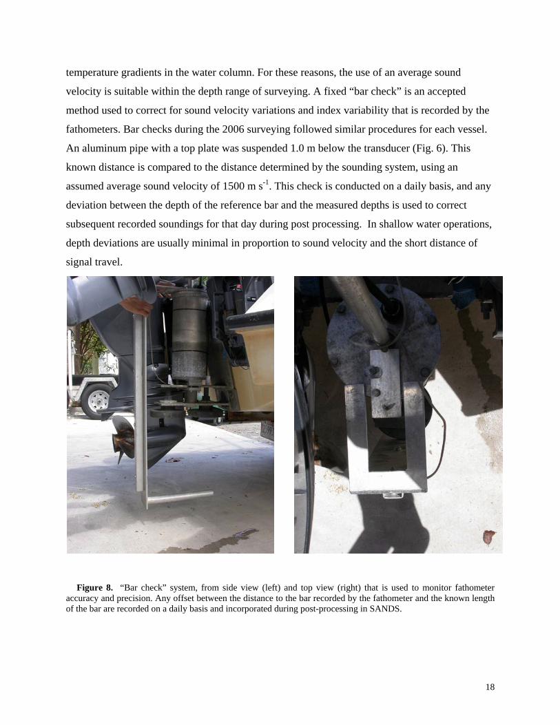
temperature gradients in the water column. For these reasons, the use of an average sound

velocity is suitable within the depth range of surveying. A fixed “bar check” is an accepted

method used to correct for sound velocity variations and index variability that is recorded by the

fathometers. Bar checks during the 2006 surveying followed similar procedures for each vessel.

An aluminum pipe with a top plate was suspended 1.0 m below the transducer (Fig. 6). This

known distance is compared to the distance determined by the sounding system, using an

assumed average sound velocity of 1500 m s-1. This check is conducted on a daily basis, and any

deviation between the depth of the reference bar and the measured depths is used to correct

subsequent recorded soundings for that day during post processing. In shallow water operations,

depth deviations are usually minimal in proportion to sound velocity and the short distance of

signal travel.

Figure 8. “Bar check” system, from side view (left) and top view (right) that is used to monitor fathometer accuracy and precision. Any offset between the distance to the bar recorded by the fathometer and the known length of the bar are recorded on a daily basis and incorporated during post-processing in SANDS.

18

GPS Percent Dilution of Position and Root Mean Square Error

The GPS antennae receive position information from the NAVSTAR satellite

constellation, which includes the Percent Dilution of Position (PDOP). PDOP is a measurement

of the relative signal strength of the GPS satellite configuration, measured internally by the GPS

system and displayed as a value typically between 1 and 4. The PDOP is a proxy for position

error, the lower the value the higher the accuracy. When PDOP readings exceeded a value of 3,

operations were halted, or data was removed from the dataset during post-processing.

During post-processing, GrafNav determines a root mean square (RMS) error for each

point based on GPS cycle slips, PDOP, satellite health, and base station RMS. Any RMS values

greater than 0.14 m were removed during quality control and assessment. After removing

outliers, the final mean RMS value was 0.07 m.

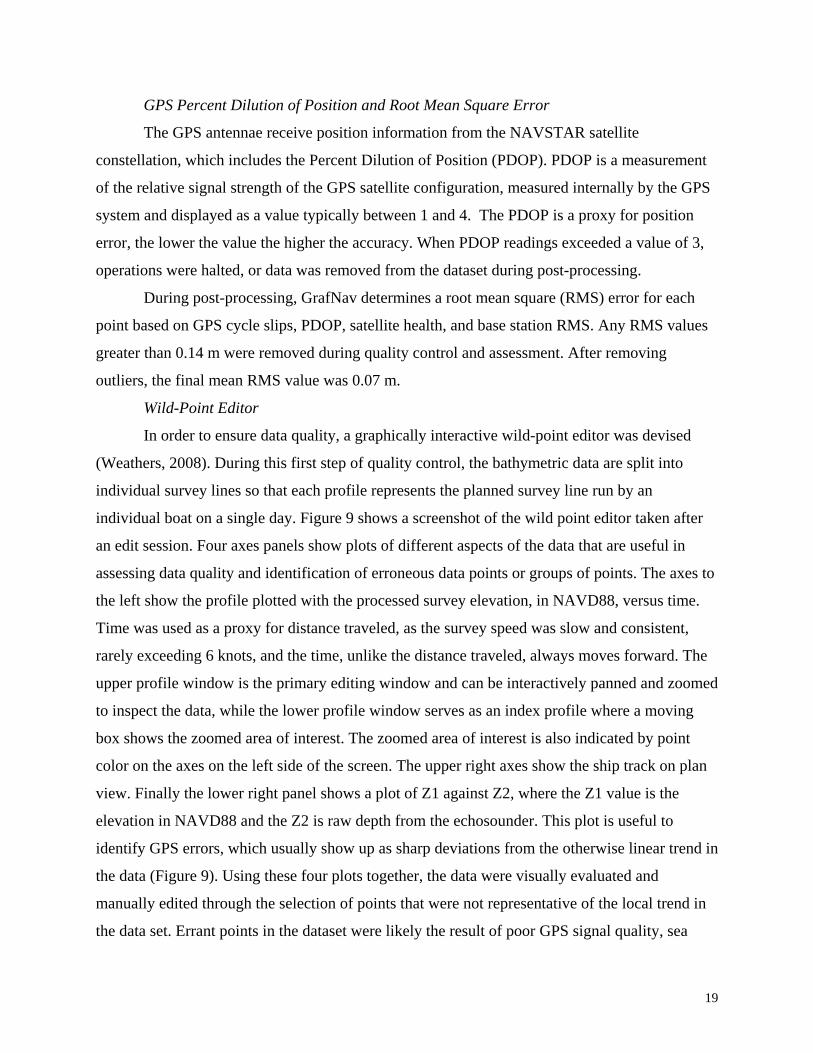
Wild-Point Editor

In order to ensure data quality, a graphically interactive wild-point editor was devised

(Weathers, 2008). During this first step of quality control, the bathymetric data are split into

individual survey lines so that each profile represents the planned survey line run by an

individual boat on a single day. Figure 9 shows a screenshot of the wild point editor taken after

an edit session. Four axes panels show plots of different aspects of the data that are useful in

assessing data quality and identification of erroneous data points or groups of points. The axes to

the left show the profile plotted with the processed survey elevation, in NAVD88, versus time.

Time was used as a proxy for distance traveled, as the survey speed was slow and consistent,

rarely exceeding 6 knots, and the time, unlike the distance traveled, always moves forward. The

upper profile window is the primary editing window and can be interactively panned and zoomed

to inspect the data, while the lower profile window serves as an index profile where a moving

box shows the zoomed area of interest. The zoomed area of interest is also indicated by point

color on the axes on the left side of the screen. The upper right axes show the ship track on plan

view. Finally the lower right panel shows a plot of Z1 against Z2, where the Z1 value is the

elevation in NAVD88 and the Z2 is raw depth from the echosounder. This plot is useful to

identify GPS errors, which usually show up as sharp deviations from the otherwise linear trend in

the data (Figure 9). Using these four plots together, the data were visually evaluated and

manually edited through the selection of points that were not representative of the local trend in

the data set. Errant points in the dataset were likely the result of poor GPS signal quality, sea

19

conditions, boat maneuvering, echosounder returns from below the seabed or from objects within

the water column, such as marine life or air bubbles.

Figure 9. Screen capture of the wild-point editor program. The two plots on the left show the soundings in profile as elevation versus time. The upper one is editable through graphical user interface. The upper right plot shows the map view of the survey transect. The lower right plot shows Z1 (GPS elevation) versus Z2 (depth from echosounder only). Points that do not plot along the Z1 vs Z2 linear trend contain GPS errors and are removed from the dataset. Data validation through crossline check

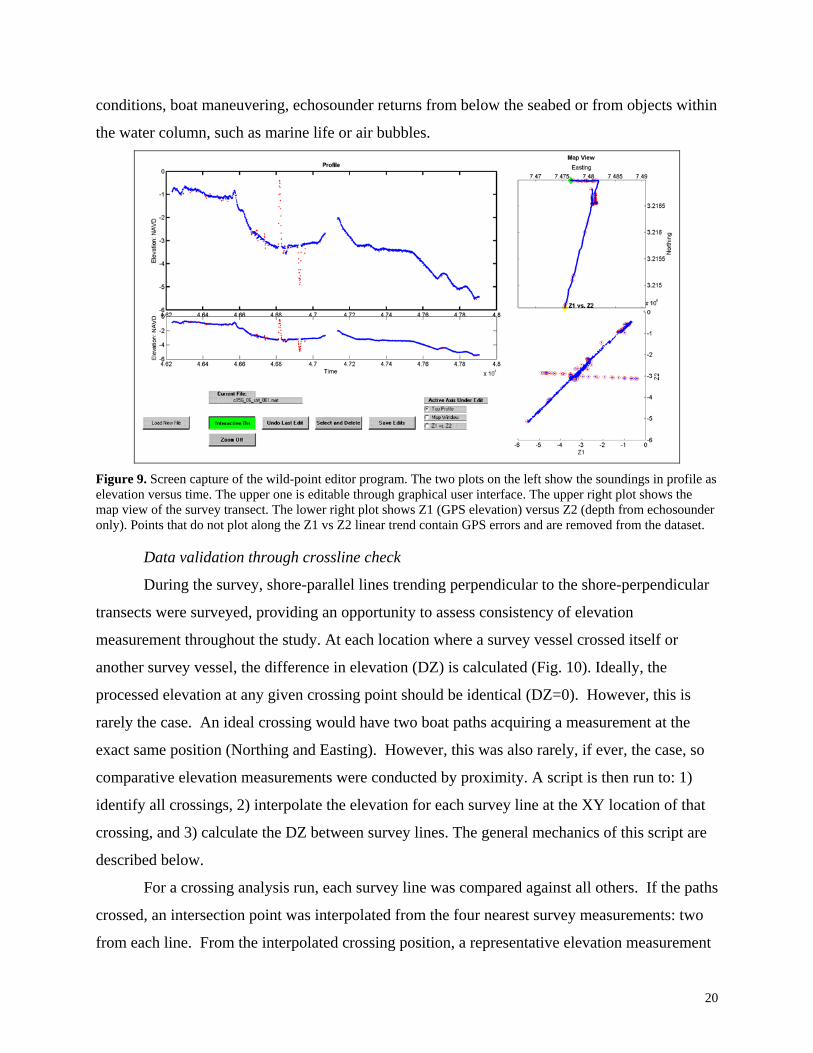
During the survey, shore-parallel lines trending perpendicular to the shore-perpendicular

transects were surveyed, providing an opportunity to assess consistency of elevation

measurement throughout the study. At each location where a survey vessel crossed itself or

another survey vessel, the difference in elevation (DZ) is calculated (Fig. 10). Ideally, the

processed elevation at any given crossing point should be identical (DZ=0). However, this is

rarely the case. An ideal crossing would have two boat paths acquiring a measurement at the

exact same position (Northing and Easting). However, this was also rarely, if ever, the case, so

comparative elevation measurements were conducted by proximity. A script is then run to: 1)

identify all crossings, 2) interpolate the elevation for each survey line at the XY location of that

crossing, and 3) calculate the DZ between survey lines. The general mechanics of this script are

described below.

For a crossing analysis run, each survey line was compared against all others. If the paths

crossed, an intersection point was interpolated from the four nearest survey measurements: two

from each line. From the interpolated crossing position, a representative elevation measurement

20

was interpolated for each boat path using an average of the measured Z (elevation) within a

given search radius of 5 m. This local averaging technique was employed in order to remove any

exaggerated DZ discrepancy that could result from an erratic Z measurement associated with any

of the four survey points used to determine the crossing position.

Boat crossing analysis is an iterative process whereby the crossing results are analyzed.

Analysis suggests problems with parts of the dataset, i.e. a miss-edited survey day, and in turn, a

way to amend this problem. The cycle of crossing analysis repeats until the data set has

desirable statistical qualities, that is, a mean DZ near 0 m and a narrow standard deviation, as this

provides an estimate of overall error in the survey point elevations. Generally, crossings identify

problems at three levels: the gross scale, the boat scale, and finally, the micro scale. The gross

scale identifies large discrepancies, those where the DZ at crossing is greater than 1 meter.

These errors are generally the result of missed edits and the like. At the boat scale, survey boat

pairs have a single mode in their DZ values; however, this value is not zero. At this scale, static

shifts are applied to the Z values in the dataset per each boat such that the DZ modes of boat

pairs all approach zero. Finally, the micro scale is where spatial trends in crossing are identified.

At this scale, individual survey days may show a general elevation difference with the rest of the

dataset that they intersect and are vertically shifted to reach better agreement.

Figure 10. Screen capture of the crossings editor program for the northern Chandeleur Islands study area. The map shows single-beam survey tracklines (black) and line crossing locations (red circles).

21

Figu

re 1

1. H

isto

gram

s out

put a

t var

ious

stag

es d

urin

g th

e Q

A/Q

C u

sing

line

cro

ssin

gs fo

r the

Rac

coon

Poi

nt to

San

dy P

oint

stud

y ar

ea. I

nitia

l run

gra

ph (t

op

left)

incl

udes

all

cros

sing

s prio

r to

any

stat

ic sh

ift (n

ote

that

bot

h x

and

y sc

ales

are

larg

er h

ere

than

on

subs

eque

nt g

raph

s). L

arge

DZ

Rem

oved

(top

righ

t) gr

aph

show

s dis

tribu

tion

of a

ll si

ngle

bea

m c

ross

ings

for a

ll th

ree

boat

s prio

r to

any

stat

ic sh

ift. O

nly

line

cros

sing

ele

vatio

n di

ffer

ence

s gre

ater

than

1m

hav

e be

en a

ddre

ssed

. The

resu

lts a

t thi

s sta

ge, a

s pre

sent

ed in

Tab

le 1

, are

use

d to

det

erm

ine

the

mos

t pre

cise

boa

t, an

d th

e va

lue

for w

hich

to sh

ift le

ss p

reci

se

boat

s to

agre

e w

ith th

e m

ost p

reci

se b

oat.

Post

Sta

tic S

hift

(low

er le

ft) h

isto

gram

is th

e di

strib

utio

n of

cro

ssin

g va

lues

afte

r the

stat

ic sh

ifts h

ave

been

app

lied.

Po

st M

icro

Adj

ustm

ent (

low

er ri

ght)

grap

h sh

ows t

he fi

nal d

istri

butio

n of

Dz

valu

es a

fter a

ddre

ssin

g sm

all e

rror

s tha

t are

line

or s

urve

y da

y sp

ecifi

c.

22

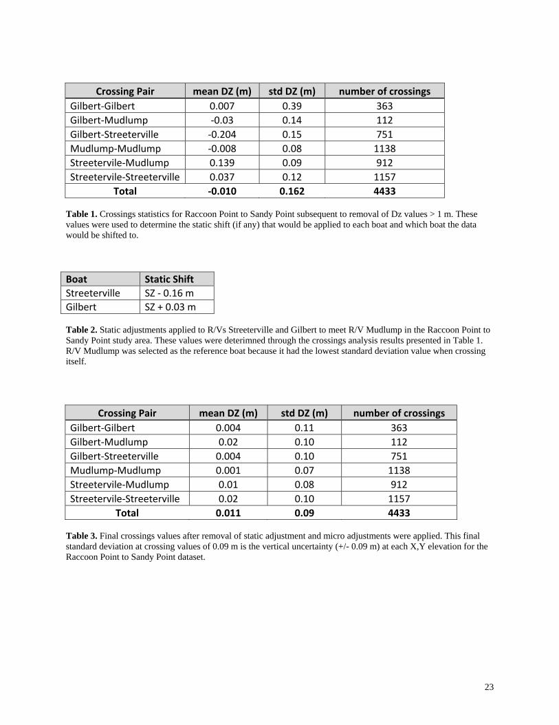
Crossing Pair  mean DZ (m)  std DZ (m)  number of crossings Gilbert‐Gilbert  0.007  0.39  363 Gilbert‐Mudlump  ‐0.03  0.14  112 Gilbert‐Streeterville  ‐0.204  0.15  751 Mudlump‐Mudlump  ‐0.008  0.08  1138 Streetervile‐Mudlump  0.139  0.09  912 Streetervile‐Streeterville  0.037  0.12  1157 

Total  ‐0.010  0.162  4433  Table 1. Crossings statistics for Raccoon Point to Sandy Point subsequent to removal of Dz values > 1 m. These values were used to determine the static shift (if any) that would be applied to each boat and which boat the data would be shifted to. Boat  Static Shift Streeterville  SZ ‐ 0.16 m Gilbert  SZ + 0.03 m  Table 2. Static adjustments applied to R/Vs Streeterville and Gilbert to meet R/V Mudlump in the Raccoon Point to Sandy Point study area. These values were deterimned through the crossings analysis results presented in Table 1. R/V Mudlump was selected as the reference boat because it had the lowest standard deviation value when crossing itself.

Crossing Pair  mean DZ (m)  std DZ (m)  number of crossings Gilbert‐Gilbert  0.004  0.11  363 Gilbert‐Mudlump  0.02  0.10  112 Gilbert‐Streeterville  0.004  0.10  751 Mudlump‐Mudlump  0.001  0.07  1138 Streetervile‐Mudlump  0.01  0.08  912 Streetervile‐Streeterville  0.02  0.10  1157 

Total  0.011  0.09  4433  Table 3. Final crossings values after removal of static adjustment and micro adjustments were applied. This final standard deviation at crossing values of 0.09 m is the vertical uncertainty (+/- 0.09 m) at each X,Y elevation for the Raccoon Point to Sandy Point dataset.

23

Figu

re 1

2. H

isto

gram

s out

put a

t var

ious

stag

es d

urin

g th

e Q

A/Q

C u

sing

line

cro

ssin

gs fo

r sou

ther

n C

hand

eleu

r Isl

ands

stud

y ar

ea. I

nitia

l run

gr

aph

incl

udes

all

cros

sing

s prio

r to

any

stat

ic sh

ift (n

ote

that

bot

h x

and

y sc

ales

are

larg

er h

ere

than

on

subs

eque

nt g

raph

s). D

Z <

1 m

eter

gra

ph

show

s dis

tribu

tion

of a

ll si

ngle

bea

m c

ross

ings

for a

ll th

ree

boat

s prio

r to

any

stat

ic sh

ift. O

nly

line

cros

sing

ele

vatio

n di

ffere

nces

gre

ater

than

1m

ha

ve b

een

addr

esse

d at

this

stag

e. T

he re

sults

at t

his s

tage

, as p

rese

nted

in T

able

4, a

re u

sed

to d

eter

min

e th

e m

ost p

reci

se b

oat,

and

the

valu

e fo

r w

hich

to sh

ift le

ss p

reci

se b

oats

to a

gree

with

the

mos

t pre

cise

boa

t. Po

st S

tatic

his

togr

am is

the

dist

ribut

ion

of c

ross

ing

valu

es a

fter t

he st

atic

sh

ifts h

ave

been

app

lied.

24

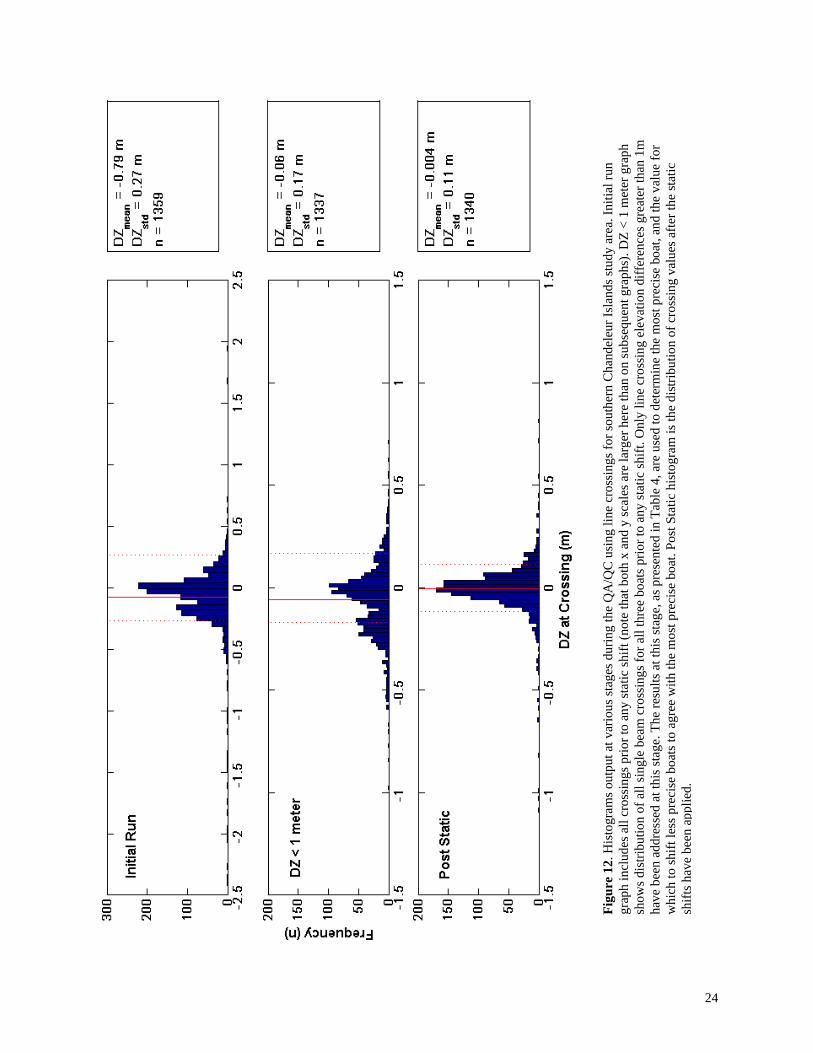
Crossing Pair  mean DZ (m)  std DZ (m)  number of crossings Gilbert‐Gilbert  ‐0.08  0.199  174 Gilbert‐Mudlump  0.034  0.124  67 Gilbert‐Streeterville  ‐0.070  0.192  242 Mudlump‐Mudlump  0.017  0.078  129 Streetervile‐Mudlump  0.188  0.104  395 Streetervile‐Streeterville  ‐0.001  0.103  333 Total Single Beam (weighted)  0.06  0.17  1340 Single Beam‐Acadiana  ‐0.16  0.11  98867 

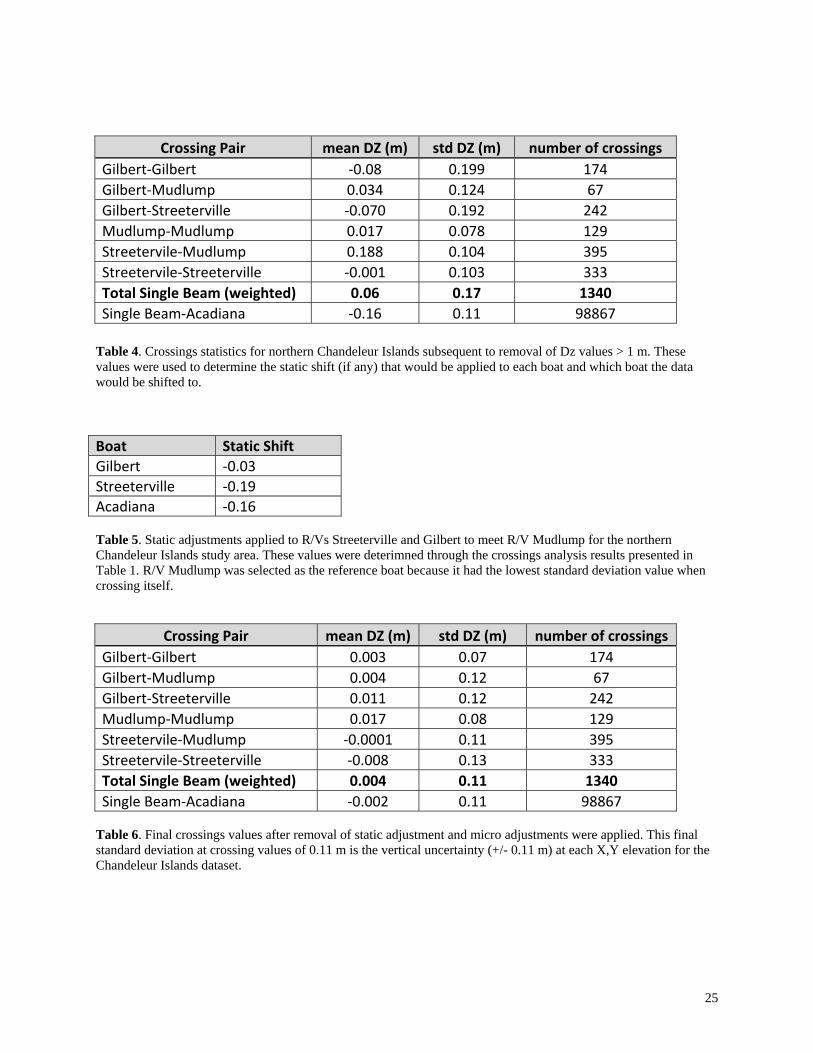
Table 4. Crossings statistics for northern Chandeleur Islands subsequent to removal of Dz values > 1 m. These values were used to determine the static shift (if any) that would be applied to each boat and which boat the data would be shifted to. Boat Static Shift Gilbert ‐0.03 Streeterville ‐0.19 Acadiana ‐0.16 Table 5. Static adjustments applied to R/Vs Streeterville and Gilbert to meet R/V Mudlump for the northern Chandeleur Islands study area. These values were deterimned through the crossings analysis results presented in Table 1. R/V Mudlump was selected as the reference boat because it had the lowest standard deviation value when crossing itself.

Crossing Pair  mean DZ (m) std DZ (m)  number of crossingsGilbert‐Gilbert  0.003  0.07  174 Gilbert‐Mudlump  0.004  0.12  67 Gilbert‐Streeterville  0.011  0.12  242 Mudlump‐Mudlump  0.017  0.08  129 Streetervile‐Mudlump  ‐0.0001  0.11  395 Streetervile‐Streeterville  ‐0.008  0.13  333 Total Single Beam (weighted)  0.004  0.11  1340 Single Beam‐Acadiana  ‐0.002  0.11  98867 

Table 6. Final crossings values after removal of static adjustment and micro adjustments were applied. This final standard deviation at crossing values of 0.11 m is the vertical uncertainty (+/- 0.11 m) at each X,Y elevation for the Chandeleur Islands dataset.

25

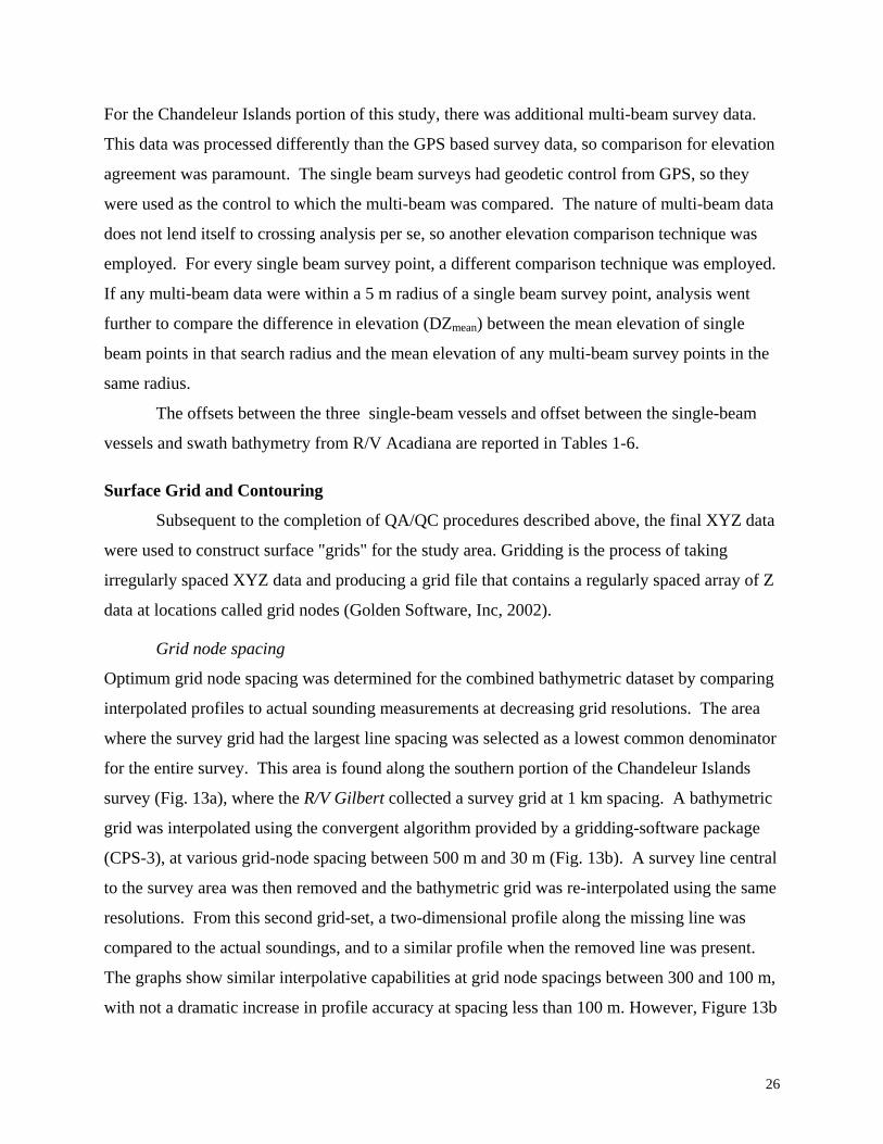
For the Chandeleur Islands portion of this study, there was additional multi-beam survey data.

This data was processed differently than the GPS based survey data, so comparison for elevation

agreement was paramount. The single beam surveys had geodetic control from GPS, so they

were used as the control to which the multi-beam was compared. The nature of multi-beam data

does not lend itself to crossing analysis per se, so another elevation comparison technique was

employed. For every single beam survey point, a different comparison technique was employed.

If any multi-beam data were within a 5 m radius of a single beam survey point, analysis went

further to compare the difference in elevation (DZmean) between the mean elevation of single

beam points in that search radius and the mean elevation of any multi-beam survey points in the

same radius.

The offsets between the three single-beam vessels and offset between the single-beam

vessels and swath bathymetry from R/V Acadiana are reported in Tables 1-6.

Surface Grid and Contouring

Subsequent to the completion of QA/QC procedures described above, the final XYZ data

were used to construct surface "grids" for the study area. Gridding is the process of taking

irregularly spaced XYZ data and producing a grid file that contains a regularly spaced array of Z

data at locations called grid nodes (Golden Software, Inc, 2002).

Grid node spacing

Optimum grid node spacing was determined for the combined bathymetric dataset by comparing

interpolated profiles to actual sounding measurements at decreasing grid resolutions. The area

where the survey grid had the largest line spacing was selected as a lowest common denominator

for the entire survey. This area is found along the southern portion of the Chandeleur Islands

survey (Fig. 13a), where the R/V Gilbert collected a survey grid at 1 km spacing. A bathymetric

grid was interpolated using the convergent algorithm provided by a gridding-software package

(CPS-3), at various grid-node spacing between 500 m and 30 m (Fig. 13b). A survey line central

to the survey area was then removed and the bathymetric grid was re-interpolated using the same

resolutions. From this second grid-set, a two-dimensional profile along the missing line was

compared to the actual soundings, and to a similar profile when the removed line was present.

The graphs show similar interpolative capabilities at grid node spacings between 300 and 100 m,

with not a dramatic increase in profile accuracy at spacing less than 100 m. However, Figure 13b

26

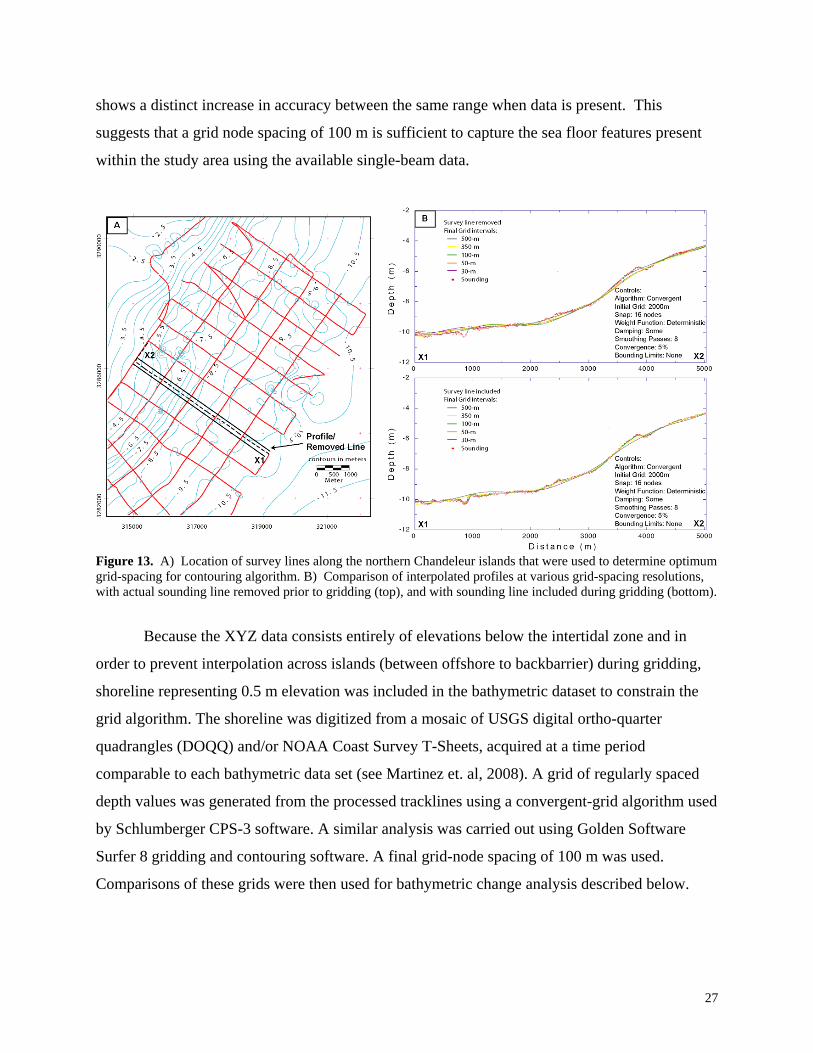
shows a distinct increase in accuracy between the same range when data is present. This

suggests that a grid node spacing of 100 m is sufficient to capture the sea floor features present

within the study area using the available single-beam data.

Figure 13. A) Location of survey lines along the northern Chandeleur islands that were used to determine optimum grid-spacing for contouring algorithm. B) Comparison of interpolated profiles at various grid-spacing resolutions, with actual sounding line removed prior to gridding (top), and with sounding line included during gridding (bottom).

Because the XYZ data consists entirely of elevations below the intertidal zone and in

order to prevent interpolation across islands (between offshore to backbarrier) during gridding,

shoreline representing 0.5 m elevation was included in the bathymetric dataset to constrain the

grid algorithm. The shoreline was digitized from a mosaic of USGS digital ortho-quarter

quadrangles (DOQQ) and/or NOAA Coast Survey T-Sheets, acquired at a time period

comparable to each bathymetric data set (see Martinez et. al, 2008). A grid of regularly spaced

depth values was generated from the processed tracklines using a convergent-grid algorithm used

by Schlumberger CPS-3 software. A similar analysis was carried out using Golden Software

Surfer 8 gridding and contouring software. A final grid-node spacing of 100 m was used.

Comparisons of these grids were then used for bathymetric change analysis described below.

27

Final grids for both historical and newly acquired bathymetric data were created in Surfer

8 and interpolated by Kriging with a 100 m grid node spacing. Kriging is a geostatistical

algorithm that uses a distance weighting, moving average and takes into account naturally

occurring regional variables that are continuous from place to place (such as a linear bar or inlet

channel), and assigns optimal weights based on the geographic arrangement of data point Z

values taken from a variogram (Davis, 1986; Krajewski and Gibbs, 2003). Kriging was

determined to be the most appropriate contouring method because it takes into account spatial

characteristics of the local geomorphology and provides the best linear estimate that can be

obtained from and irregular arrangement of data samples. A linear variogram model with no

nugget effect was used.

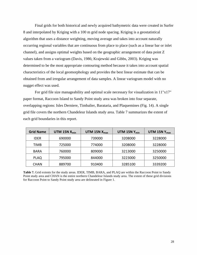
For grid file size manageability and optimal scale necessary for visualization in 11"x17"

paper format, Raccoon Island to Sandy Point study area was broken into four separate,

overlapping regions: Isles Derniere, Timbalier, Barataria, and Plaquemines (Fig. 14). A single

grid file covers the northern Chandeleur Islands study area. Table 7 summarizes the extent of

each grid boundaries in this report.

Grid Name  UTM 15N Xmin  UTM 15N Xmax  UTM 15N Ymin  UTM 15N Ymax 

IDER  690000  739000  3208000  3228000 

TIMB  725000  774000  3208000  3228000 

BARA  760000  809000  3213000  3250000 

PLAQ  795000  844000  3223000  3250000 

CHAN  889700  910400  3285100  3339200  Table 7. Grid extents for the study areas. IDER, TIMB, BARA, and PLAQ are within the Raccoon Point to Sandy Point study area and CHAN is the entire northern Chandeleur Islands study area. The extent of these grid divisions for Raccoon Point to Sandy Point study area are delineated in Figure 1.

28

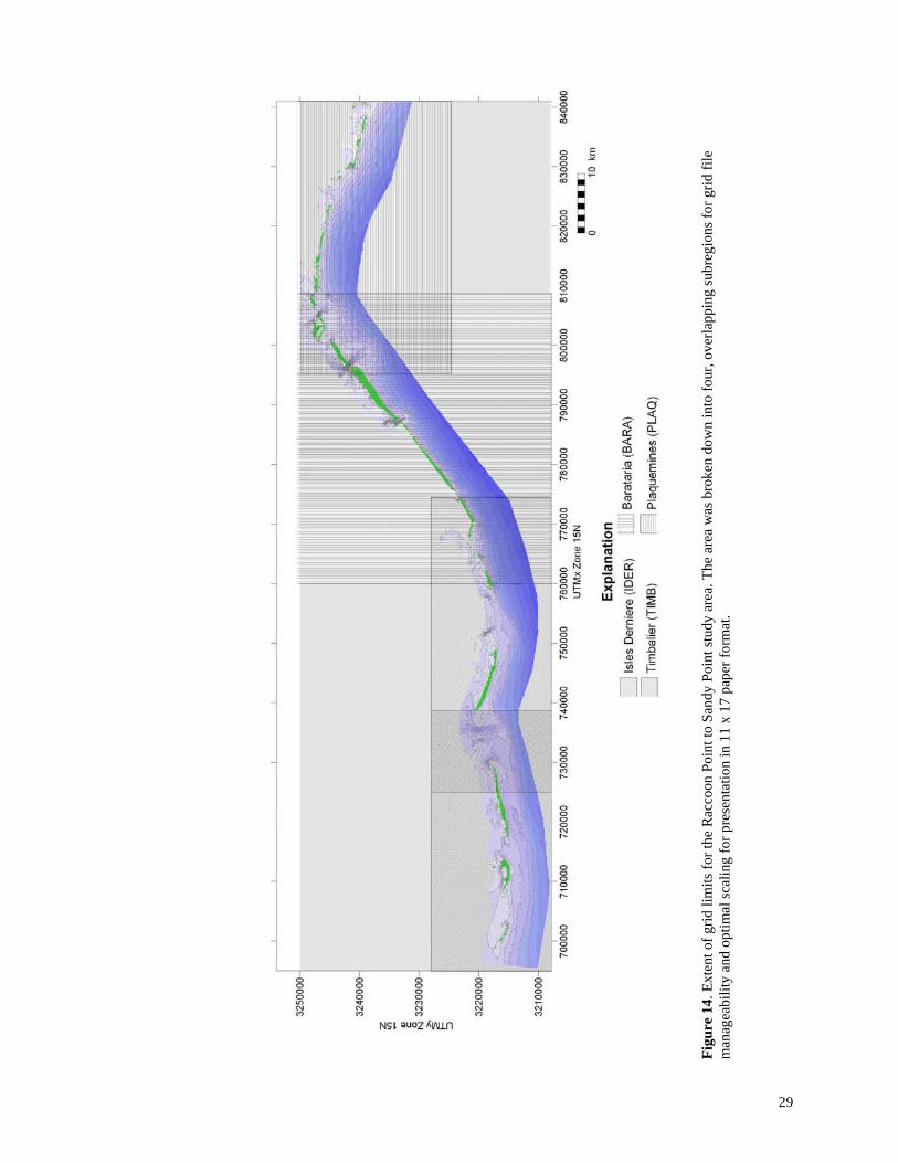
Figu

re 1

4. E

xten

t of g

rid li

mits

for t

he R

acco

on P

oint

to S

andy

Poi

nt st

udy

area

. The

are

a w

as b

roke

n do

wn

into

four

, ove

rlapp

ing

subr

egio

ns fo

r grid

file

m

anag

eabi

lity

and

optim

al sc

alin

g fo

r pre

sent

atio

n in

11

x 17

pap

er fo

rmat

.

29

HISTORICAL BATHYMETRIC DATA COLLECTION

Northern Chandeleur Islands

1873 - 1885

U.S. Coast and Geodetic Survey (USCGS) hydrographic survey smooth sheets or H-

sheets were acquired through the Hydrographic Survey Division of NOAA's Office of Coast

Survey as high-resolution scanned image files (.tif and .jpg). H-sheets used for this analysis

consist of H01171 (1873) and H01654 (1885). The H-sheets were originally referenced to a

geographical (latitude/longitude) coordinate system based on the Clarke 1866 ellipsoid model.

NAD27 control points were added to the sheets by the USCGS in the 1930's. The depth

soundings are reported relative to MLW at the time of the survey, and are therefore referenced to

an arbitrary vertical datum. Horizontal positioning for the soundings was accomplished by means

of recording sextant angles from the ship to known landmarks, recording theodolite angles to the

survey vessel from the shoreline positions, and dead reckoning (estimation of position based on

ship speed and heading) (List et al., 1994).

In order to project the H-sheet images for digitizing, a grid to a known datum (NAD27)

had to be overlain on the image. The geographic coordinate grid from the original H-sheet was

traced in Adobe Illustrator. The traced coordinate grid was then shifted to match the NAD27

control point on the H-sheet. The shifted coordinate grid overlain on the H-sheet was saved as a

single layer tif file. ERDAS IMAGINE software was then used to establish a series of

geographic control points at the coordinate grid intersections in order to georectify the image for

projection in GIS software applications. Over 65 control points for each H-sheet were digitized

in NAD27 using ERDAS IMAGINE's Geographic Control Point (GCP) tool. On each H-sheet,

an outline of the shoreline that was traced from a USCGS Topographic Survey smooth sheet (T-

sheet) was compared to a shoreline polygon in ESRI ArcGis 9.2 that had been previously

digitized from a T-sheet and was acquired from NOAA. This served as a quality assessment of

digitizing and projection accuracy.

The bathymetric soundings on each projected and rectified h-sheet were then digitized

on-screen using ESRI ArcGis 9.2. After digitizing, the soundings were converted from feet and

fathoms into meters. Horizontal data was converted from geographic NAD27 into UTM Zone 15

North NAD83 using CORPSCON 6.0. Files in XYZ format were then produced for gridding.

30

1917-1922

The 1920 data was acquired digitally from the Hydrographic Survey Division of NOAA's

Office of Coast Survey. Surveys used to produce the bathymetric maps included H04000 (1917),

H04171 (1920), H04212 (1921-1922), and H04219 (1922). The smooth sheets associated with

these surveys were digitized between 2001 and 2004 by a NOS contactor. The data was

downloaded as an XYZ file referenced to NAD83 with soundings expressed in meters relative to

MLW at the time of the survey.

Horizontal positioning was achieved by using a system of triangulation based on a series

of towers (up to 100 ft high) and base stations located along the Chandeleur Islands. Beyond the

limit of sight from the shoreline, buoys located using cuts and fixes from the shore signal were

placed at the outer limit of the planned survey lines. Soundings were acquired using sextant

three-point fixes for horizontal positioning when in sight of the positioning signals, and dead

reckoning when signals were out of sight. A hand lead was used to a depth of 15 fathoms. From

the 15 fathom to the 25 fathom depth a trolley rig consisting of a leadline with copper core. In

depths greater than 25 fathoms, a mechanical sounding machine was used. A tidal staff at the

Chandeleur Island light, along with automatic tide gauges at Bay St. Louis and Biloxi,

Mississippi and Ft. Morgan, Alabama were used to correct soundings to a common datum of

MLW (Summarized from USCGS, 1917; 1920; 1922; Hawley, 1931).

Raccoon Point to Sandy Point

Historical bathymetric data was acquired in digital form from the USGS and was

published by the USGS and Louisiana Geological Survey titled Louisiana Barrier Island Erosion

Study: Atlas of Seafloor Changes from 1878 to 1989 by List et al. (1994). Jaffe et al. (1991) and

List et al. (1994) discuss extensively the methods employed for data collection, cartographic

production, and seafloor change analysis. The data for this region is broken down into three time

periods; the 1880's, 1930's, and 1980's.

The historical data acquired for this region was horizontally referenced to NAD27 a

conversion to NAD83 was necessary. This was done using CORPSCON6 transformation

software available from USACE. The vertical datum in which these data were referenced to was

MLW or MLLW at the time of each survey. In order to bring these data into a comparable

31

vertical reference frame, they were shifted to NAVD88. This transformation process is discussed

in the following section.

ADJUSTMENT OF HISTORICAL VERTICAL DATA TO NAVD88

A subsequent report (BICM Vol. 3, Part 3) will include a seafloor change analysis by

comparing grids from two different time periods in order to determine erosion and accretion

patterns and sediment transport trends. In order to compare surfaces from two different time

periods, they must be referenced to a common vertical datum. This proposed a problem in the

study area because much of the historical data is referenced to an arbitrary datum, mean low

water (MLW) at the time of the survey. Because relative sea level rise (RSLR) rates are so high

in the study area, the MLW elevation is constantly increasing. This problem was encountered by

List et al. (1994) when attempting to perform seafloor change analysis in Louisiana. The reader

is referred to Jaffe et al. (1991) and List et al. (1994) for extensive discussion on the methods

employed for accounting for RSLR in Louisiana. The 1880's and 1930's bathymetric data in this

study, is shifted for RSLR using a correction determined by Jaffe et al. (1991). This method

involved the identification of a area of seafloor, seaward of the shoreface, that undergoes

relatively no erosion or accretion, and therefore the bathymetric change in that area is the result

of RSLR. The surface for each year (1880's and 1930's) was shifted based on the RSLR

estimated from the area of no seafloor change. The shift for each year, as determined by Jaffe et

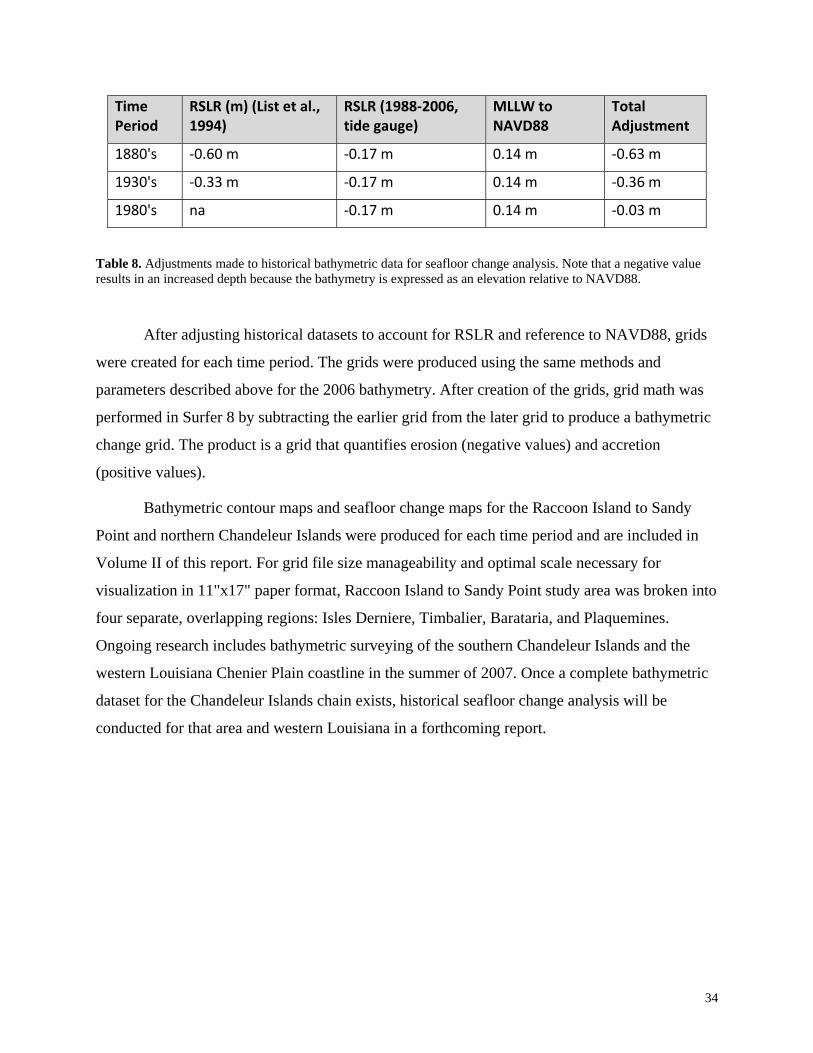
al. (1991) was 0.33 m between 1930 and 1980, and 0.27 m between 1880 and 1930 (Table 8).

For the seafloor change portion of this study, all of the historical data was shifted to

reference an elevation relative to NAVD88 for comparison to the 2006 bathymetry. There were

two steps to this process. The first involved shifting each bathymetric dataset to a common

datum that also takes into account the RSLR that occurred between each time period. Each of the

historical datasets were shifted to MLLW at Grand Isle for the 1983-2001 tidal epoch. This

involved a using the shifts determined by Jaffe et al. (1991) and List et al. (1994) for the 1880's

and 1930's, plus a shift applied to the 1980's data for comparison to 2006. The RSLR rate for the

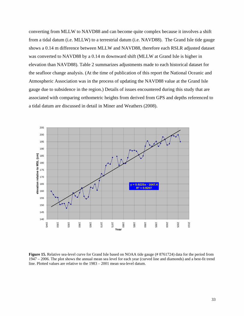
1980-2006 time period was determined from the long-term rate of RSLR based on the Grand Isle

tide gauge (0.92 cm/yr for the period from 1947-2006; Fig. 15). This shift was then applied to all

of the historical data, plus any shift previously determined for each year by Jaffe et al. (1991)

and List et al. (1994) to arrive at MLLW for 2006. The second part of the process involved

32

converting from MLLW to NAVD88 and can become quite complex because it involves a shift

from a tidal datum (i.e. MLLW) to a terrestrial datum (i.e. NAVD88). The Grand Isle tide gauge

shows a 0.14 m difference between MLLW and NAVD88, therefore each RSLR adjusted dataset

was converted to NAVD88 by a 0.14 m downward shift (MLLW at Grand Isle is higher in

elevation than NAVD88). Table 2 summarizes adjustments made to each historical dataset for

the seafloor change analysis. (At the time of publication of this report the National Oceanic and

Atmospheric Association was in the process of updating the NAVD88 value at the Grand Isle

gauge due to subsidence in the region.) Details of issues encountered during this study that are

associated with comparing orthometric heights from derived from GPS and depths referenced to

a tidal datum are discussed in detail in Miner and Weathers (2008).

y = 0.9225x - 1647.4R2 = 0.9207

140

145

150

155

160

165

170

175

180

185

190

195

200

205

1945

1950

1955

1960

1965

1970

1975

1980

1985

1990

1995

2000

2005

2010

elev

atio

n re

lativ

e to

MSL

(cm

)

Year

Figure 15. Relative sea-level curve for Grand Isle based on NOAA tide gauge (# 8761724) data for the period from 1947 – 2006. The plot shows the annual mean sea level for each year (curved line and diamonds) and a best-fit trend line. Plotted values are relative to the 1983 – 2001 mean sea-level datum.

33

Time Period 

RSLR (m) (List et al., 1994) 

RSLR (1988‐2006, tide gauge) 

MLLW to NAVD88 

Total Adjustment 

1880's  ‐0.60 m  ‐0.17 m  0.14 m  ‐0.63 m 

1930's  ‐0.33 m  ‐0.17 m  0.14 m  ‐0.36 m 

1980's  na  ‐0.17 m  0.14 m  ‐0.03 m 

 

Table 8. Adjustments made to historical bathymetric data for seafloor change analysis. Note that a negative value results in an increased depth because the bathymetry is expressed as an elevation relative to NAVD88.

After adjusting historical datasets to account for RSLR and reference to NAVD88, grids

were created for each time period. The grids were produced using the same methods and

parameters described above for the 2006 bathymetry. After creation of the grids, grid math was

performed in Surfer 8 by subtracting the earlier grid from the later grid to produce a bathymetric

change grid. The product is a grid that quantifies erosion (negative values) and accretion

(positive values).

Bathymetric contour maps and seafloor change maps for the Raccoon Island to Sandy

Point and northern Chandeleur Islands were produced for each time period and are included in

Volume II of this report. For grid file size manageability and optimal scale necessary for

visualization in 11"x17" paper format, Raccoon Island to Sandy Point study area was broken into

four separate, overlapping regions: Isles Derniere, Timbalier, Barataria, and Plaquemines.

Ongoing research includes bathymetric surveying of the southern Chandeleur Islands and the

western Louisiana Chenier Plain coastline in the summer of 2007. Once a complete bathymetric

dataset for the Chandeleur Islands chain exists, historical seafloor change analysis will be

conducted for that area and western Louisiana in a forthcoming report.

34

REFERENCES Barras, J., Beville, S., Britsch, D., Hartley, S., Hawes, S., Johnston, J., Kemp, P., Kinler, Q., Martucci, A.,   Porthouse, J., Reed, D., Roy, K., Sapkota, S., and Suhayda, J., 2003, Historical and Projected      39 p. (Revised January 2004).  Davis, J. C., 1986, Statistics and Data Analysis in Geology, Second Edition: New York, John Wiley and   Sons, 646 p.  Golden Software, Inc., 2002, Surfer 8 Contouring and 3D Surface Mapping for Scientists and Engineers   User's Guide: Golden, Colorado, Golden Software, Inc., 640 p.  Hawley, J. H., 1931, Hydrographic Manual: Washington, D.C., Department of Commerce, U.S. Coast and   Geodetic Survey, Special Publication no. 143, 170 p.  Jaffe, B., List, J., Sallenger, A., Jr., and Holland, T., 1991, Louisiana Barrier Island Erosion Study:   Correction for the Effect of Relative Sea Level Change on Historical Bathymetric Survey   Comparisons, Isles Derniere Area, Louisiana: Reston, Virginia, U.S. Geological Survey, Open‐file   report  91‐276, 33 p.   Krajewski, S. A. and Gibbs, B. L., 2003, Understanding Computer Contouring: Boulder, Gibbs and   Associates, poster, 1 sheet.   List, J. H., Jaffe, B. E., Sallenger, A. H., Jr.,Williams, S. J.,McBride, R. A., and Penland, S., 1994, Louisiana   Barrier Island Erosion Study: Atlas of Seafloor Changes from 1878 to 1989: Reston, Virginia, U.S.   Geological Survey and Louisiana State University, Miscellaneous Investigations Series I‐2150‐A,   81p.  Louisiana Coastal Area, 2004, Louisiana Coastal Area, Louisiana Ecosystem Restoration Study, Final   Report, 4 volumes with appendices, http://www.lca.gov/final_report.aspx, accessed June 2008. 

 Martinez, L., Penland, S., Fernley, S., O'Brien, S., Bethel, M., and Guarisco, P., 2009, Louisiana Barrier   Island Comprehensive Monitoring Program (BICM), Volume 2: Shoreline Changes and Barrier   Island Land Loss 1800’s‐2005: Pontchartrain Institute for Environmental Sciences, University of   New Orleans, New Orleans, Louisiana, Report Submitted to Louisiana Department of Natural   Resources, 5 parts and appendices.   Miner, M. D. and Weathers, H. D., in press, Adjustment of Tidally‐Referenced Water Depths for Comparison to   GPS‐Derived Orthometric Heights in the Louisiana Coastal Zone: Pontchartrain Institute for   Environmental Sciences, Tecnical Report no. 003‐2008, University of New Orleans, New Orleans,   Louisiana, p  Penland, S. and Ramsey, K. E., 1990, Relative Sea Level Rise in Louisiana and the Gulf of Mexico; 1908‐  1988: Journal of Coastal Research, v. 6, 323 ‐342.  

35

U.S. Coast and Geodetic Survey, 1917, Descriptive Report for Hydrographic Survey Sheet No. 4000, Gulf   of Mexico, Mississippi Sound: Washington, D.C., Department of Commerce, U.S. Coast and   Geodetic Survey, 7 p.   U.S. Coast and Geodetic Survey, 1920, Descriptive Report for Hydrographic Survey Sheet No. 4171, Gulf   of Mexico, Mobile Bay Entrance to Chandeleur Islands Offshore: Washington, D.C., Department   of Commerce, U.S. Coast and Geodetic Survey, 13 p.   U.S. Coast and Geodetic Survey, 1922, Descriptive Report for Hydrographic Survey Sheet No. 4219,   Chandeleur Sound, North, Freemason, and Old Harbor Islands: Washington, D.C., Department of   Commerce, U.S. Coast and Geodetic Survey, 9 p.   Weathers, H. D., in press, Graphical Interface Method for Editing GPS‐Derived Bathymetric Data Points:   Pontchartrain Institute for Environmental Sciences, Tecnical Report no. 003‐2009, University of   New Orleans, New Orleans, Louisiana.  Williams, S. J., Penland, S., and Sallenger, A. H., Jr., 1992, Louisiana Barrier Island Erosion Study, Atlas of   Shoreline Changes in Louisiana from 1853 to 1989: Reston, Virginia, U.S. Geological Survey and   Louisiana State University, Miscellaneous Investigations Series I‐2150‐A, 103 p.  

36

APPENDIX A: GLOSSARY

Benchmark A fixed solid reference point with a precisely determined published elevation CORS (Continually Operating Reference Station) An NGS maintained GPS station that is part of a the larger CORS network. The CORS network provides carrier phase and code range measurements in support of 3-dimensional positioning activities throughout the United States. Cut The measurement down from a grade mark Datum A fixed reference for horizontal and vertical measurements (i.e. NAD83 or NAVD88) Dead Reckoning The process of estimating position based upon a previously determined position (fix) and advancing that position based upon known speed, elapsed time, and course. Ellipsoid A mathematically-defined surface that approximates the geoid. Fix A position derived from measuring external reference points. Geographic Information System (GIS) A system for storing, analyzing, and managing data which are spatially referenced to Earth Geoid A surface that is approximately represented by mean sea level is the equipotential surface of the Earth's gravity field. Global Positioning System (GPS) A ground positioning (X, Y, and Z) technique based on the reception and analysis of NAVSTAR satellite signals. Grid a file that contains a regularly spaced array of Z data at locations called grid nodes developed by interpolating between irregularly spaced XYZ data. H-Sheet Term for a U.S. Coast and Geodetic Survey hydrographic sheet that show soundings from a hydrographic survey. Interferometric Swath Bathymetry A sonar system that is used to measure the depth in a line extending outwards from the sonar transducer. Data is acquired in a swath at right angles to the direction of vessel motion. In contrast to traditional multibeam echo sounders ‘interferometry” is generally used to describe swath-sounding sonar techniques that use the phase content of the sonar signal to measure the angle of a wave front returned from a sonar target. When backscattered sound energy is received back at the transducer, the angle return ray of acoustic energy makes with the transducer is measured. The range is calculated from the two-way travel time. The angle is determined by knowing the spacing between elements within the transducer, the phase difference of the incoming wave front, and the wavelength (Submetrix 2000 Series Training Pack, 2000, Submetrix Ltd., Bath, U.K.). Kriging a geostatistical algorithm that uses a distance weighting, moving average and takes into account naturally occurring regional variables that are continuous from place to place (such as a linear bar or inlet channel), and assigns optimal weights based on the geographic arrangement of data point Z values taken from a variogram Mean High Water (MHW) A tidal datum defined by the average of all the high water heights observed over a tidal epoch.

37

Mean Low Water (MLW) A tidal datum defined by the average of all the low water heights observed over a tidal epoch. Mean Lower Low Water (MLLW) A tidal datum defined by the average of the lower low water height each tidal day observed over a tidal epoch. NAVSTAR A set of orbiting satellites used in navigation and positioning. North American Datum 1927 (NAD27) A geodetic horizontal datum based on the Clarke 1866 Ellipsoid. North American Datum 1983 (NAD83) A geodetic horizontal datum based on the GRS80 Ellipsoid North American Vertical Datum 1988 (NAVD88) Vertical control datum established in 1991 by the minimum constraint adjustment of geodetic leveling observations in North America. Online Position User Service (OPUS) A web-based GPS solution engine hosted by the Natioinal Geodetic Survey (NGS). GPS files can be submitted to the NGS and each file is processed with respect to three CORS sites. A position is then reported back to the user via email. http://www.ngs.noaa.gov/OPUS/ Orthometric Height (H) The distance from the geoid surface to the ground surface. Also known as elevation. Kinematic GPS Survey A GPS survey that consists of a base station and roving unit occupying a 15-km or less baseline. Sextant A measuring instrument that is used to measure the angle of elevation of a celestial object above the horizon. The angle and time when it was measured can be used to calculate a position line on a nautical chart. Side Scan Sonar Single-Beam Bathymetry depth sounding that uses a high frequency acoustic pulse directed downward in the water column. Acoustic energy is reflected off of the seafloor beneath the survey vessel and recorded at the transceiver. A continuous recording of water depth below the vessel produces high resolution measurements along the survey transect. T-Sheet Term for a U.S. Coast and Geodetic Survey topographic sheet that shows shoreline position and land elevation based on a topographic survey. Theodolite An instrument for measuring both horizontal and vertical angles as used in triangulation networks. Tidal Inlet A channel that is flanked by barrier islands and is a conduit for daily tidal exchange between the lagoon or marsh and the open ocean (Gulf). Tidal inlet channels are maintained by tidal currents by flushing sand transported into the channel by wave processes. Tidal Staff A portable water level measuring device used to determine local tidal datums. Triangulation A control survey in which the coordinates and distance to a point are determined by calculating the length of one side of a triangle, given measurements of angles and sides of the triangle formed by that point and two other known reference points using the law of sines. Variogram Model mathematically specifies the spatial variability of the dataset and the resulting grid file.

38

Appendix B: GPS Base Station Session Results and Positions Used for this Study

39

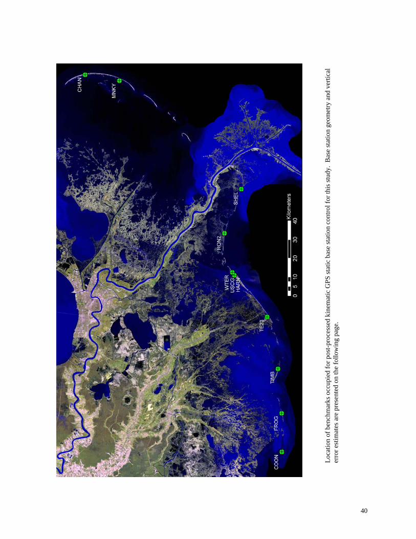
Loca

tion

of b

ench

mar

ks o

ccup

ied

for p

ost-p

roce

ssed

kin

emat

ic G

PS st

atic

bas

e st

atio

n co

ntro

l for

this

stud

y. B

ase

stat

ion

geom

etry

and

ver

tical

er

ror e

stim

ates

are

pre

sent

ed o

n th

e fo

llow

ing

page

.

40

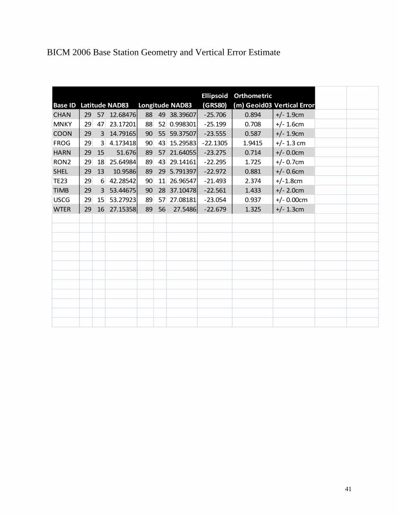
BICM 2006 Base Station Geometry and Vertical Error Estimate

Base ID Latitude NAD83 Longitude NAD83Ellipsoid (GRS80)

Orthometric (m) Geoid03 Vertical Error

CHAN 29 57 12.68476 88 49 38.39607 ‐25.706 0.894  +/‐ 1.9cm MNKY 29 47 23.17201 88 52 0.998301 ‐25.199 0.708  +/‐ 1.6cm COON 29 3 14.79165 90 55 59.37507 ‐23.555 0.587  +/‐ 1.9cm FROG 29 3 4.173418 90 43 15.29583 ‐22.1305 1.9415  +/‐ 1.3 cm HARN 29 15 51.676 89 57 21.64055 ‐23.275 0.714  +/‐ 0.0cm RON2 29 18 25.64984 89 43 29.14161 ‐22.295 1.725  +/‐ 0.7cm SHEL 29 13 10.9586 89 29 5.791397 ‐22.972 0.881  +/‐ 0.6cm TE23 29 6 42.28542 90 11 26.96547 ‐21.493 2.374  +/‐1.8cm TIMB 29 3 53.44675 90 28 37.10478 ‐22.561 1.433  +/‐ 2.0cm USCG 29 15 53.27923 89 57 27.08181 ‐23.054 0.937  +/‐ 0.00cm WTER 29 16 27.15358 89 56 27.5486 ‐22.679 1.325  +/‐ 1.3cm

41