bayesian ivice.uchicago.edu/2008_presentations/rossi/stanford_mkt.pdfmotivation iv problems are...
TRANSCRIPT
Bayesian IV
Peter RossiGSB/U of ChicagoGSB/U of Chicago
joint with Rob McCulloch, Tim Conley, and j yChris Hansen

MotivationIV problems are often done with a “small” amount
f l f ( k/ )of sample information (weak/many instruments).
It would seem natural to apply a small amount of i i f ti i l ti iti lik l prior information, e.g. price elasticities are unlikely
to be outside (-1,-5).
Another nice example instruments are not exactly Another nice example– instruments are not exactly valid. They have some small direct correlation with the outcome/unobservables.
BUT, Bayesian methods (until now) are tightly parametric. Do I always have to make the efficiency/consistency tradeoff as in std IV?
2
efficiency/consistency tradeoff as in std IV?

OverviewConsider parametric (normal) model first
Consider finite mixture of normals for error dist
Make the number of mixture components random pand possibly “large”
Conduct sampling experiments and compare to state of the art classical methods of inference
Consider some empirical examples where being a i B i h l !non-parametric Bayesian helps!
Show how a Bayesian would deal with instruments that are not strictly valid
3
that are not strictly valid.
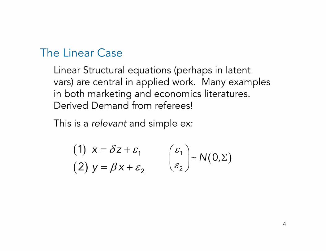
The Linear CaseLinear Structural equations (perhaps in latent
) l l d k lvars) are central in applied work. Many examples in both marketing and economics literatures. Derived Demand from referees!
This is a relevant and simple ex:
( )( )
= +
= +1
2
1
2
x z
y x
δ εβ ε
( )⎛ ⎞Σ⎜ ⎟
⎝ ⎠
1
2
~ 0,Nεε( ) 2
4
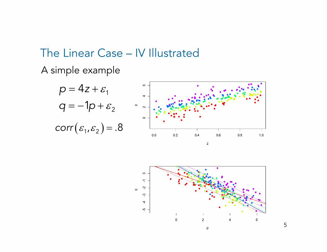
The Linear Case – IV IllustratedA simple example
εε
= += − +
1
2
41
p zq p 2q p
( )ε ε =1 2, .8corr
5
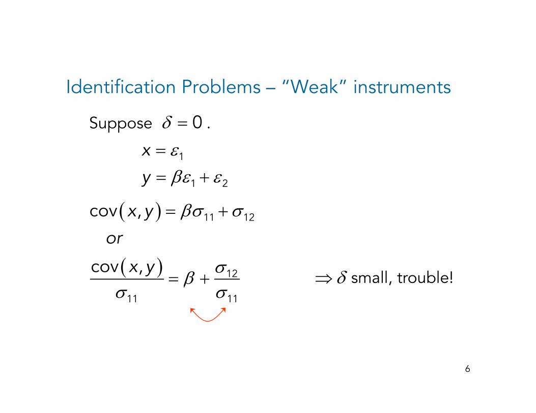
Identification Problems – “Weak” instruments
Suppose . = 0δS pp
== +
1
1 2
xy
εβε ε+1 2y βε ε
( ) = +11 12cov ,x y βσ σ
( ) = + 12cov ,
or
x y σβ small, trouble! ⇒δ11 11
βσ σ
,
6
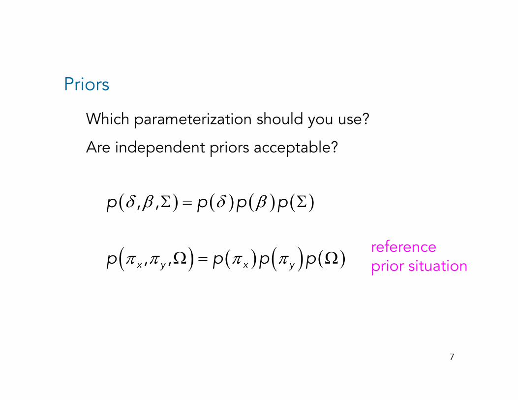
Priors
Which parameterization should you use? p y
Are independent priors acceptable?
( ) ( ) ( ) ( )δ β δ βΣ = Σ, ,p p p p
( ) ( ) ( ) ( )π π π πΩ = Ω, ,x y x yp p p preference prior situation
7
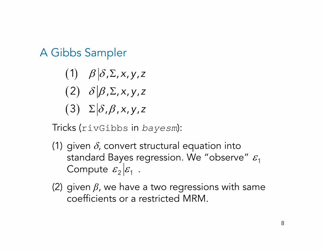
A Gibbs Sampler
( ) Σ1 , , , ,x y zβ δ( )( )( )
Σ
Σ
, , , ,
2 , , , ,
3
y
x y z
x y z
β
δ β
δ β
Tricks (rivGibbs in bayesm):
( ) Σ3 , , , ,x y zδ β
(1) given δ, convert structural equation into standard Bayes regression. We “observe” Compute .
1ε2 1ε εCo pute
(2) given β, we have a two regressions with same coefficients or a restricted MRM.
2 1
8
1.0
0
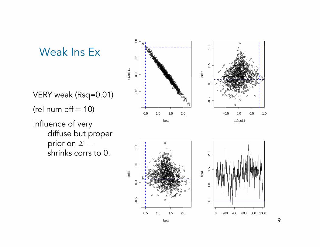
Weak Ins Ex
0.0
0.5
2os1
1
0.5
1.0
delta
VERY weak (Rsq=0.01)
( l ff 10)
-0.5
s1
-0.5
0.0
d
(rel num eff = 10)
Influence of very diffuse but proper
0.5 1.0 1.5 2.0
beta
-0.5 0.0 0.5 1.0
s12os11
prior on Σ --shrinks corrs to 0.
0.5
1.0
.52.
0
0.5
0.0
delta
.51.
01
beta
90.5 1.0 1.5 2.0
-0
beta
0 200 400 600 800 10000
0
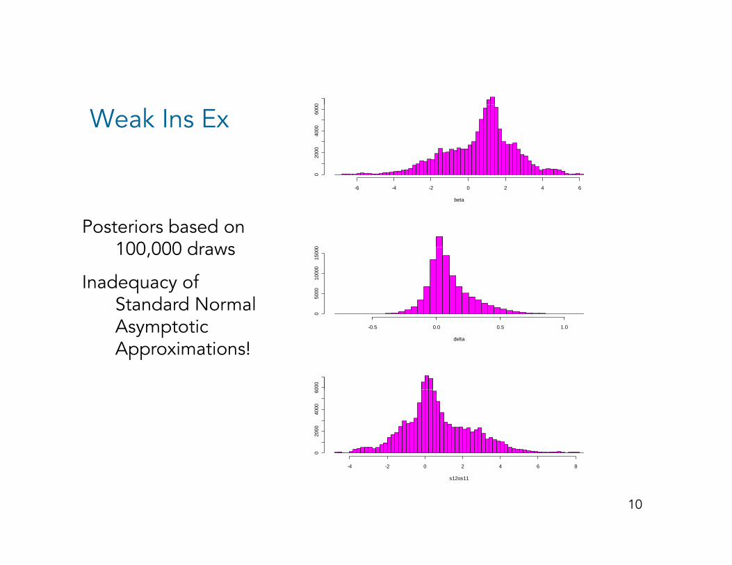
Weak Ins Ex
020
0040
0060
00
Posteriors based on 100 000 draws
beta
-6 -4 -2 0 2 4 6
0100,000 draws
Inadequacy of Standard Normal
050
0010
000
1500
0
Asymptotic Approximations!
delta
-0.5 0.0 0.5 1.0
000
020
0040
0060
10
s12os11
-4 -2 0 2 4 6 8

Mixtures of Normal for Errors
Consider the instrumental variables model with
= + '1x zδ ε
mixture of normal errors with K components:
+
= +
⎛ ⎞
1
'2
'
x z
y x
δ ε
β ε
( )⎛ ⎞Σ⎜ ⎟
⎝ ⎠
1'2
~ ,ind indNε
με
~ ( )ind multinomial p
⎡ ⎤⎡ ⎤ = ⎡ ⎤ =⎣ ⎦ ⎣ ⎦⎣ ⎦ ∑' '1
note: E and EK
ind k kkind E ind pε μ ε μ
11
=⎡ ⎤ ⎡ ⎤⎣ ⎦ ⎣ ⎦⎣ ⎦ ∑ 1ind k kk
pμ μ
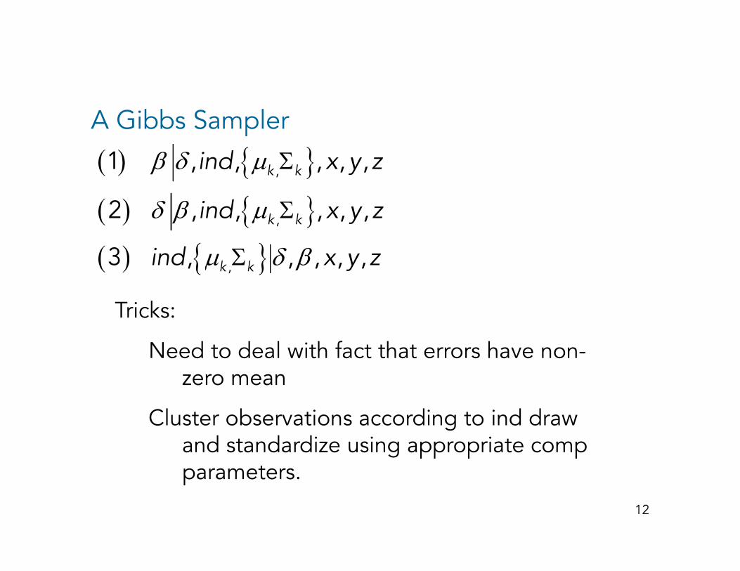
A Gibbs Sampler
( ) { }Σ,1 , , , , ,k kind x y zβ δ μ{ }( ) { }( ) { }
Σ
Σ
,2 , , , , ,
3
k kind x y z
i d
δ β μ
δ β
Tricks:
( ) { }Σ,3 , , , , ,k kind x y zμ δ β
Need to deal with fact that errors have non-zero mean
Cluster observations according to ind draw and standardize using appropriate comp
t
12
parameters.
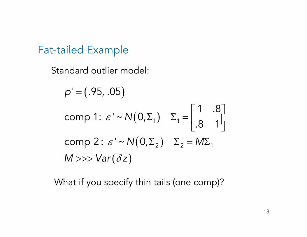
Fat-tailed Example
Standard outlier model:
( )=' .95, .05p
( ) ⎡ ⎤Σ Σ = ⎢ ⎥
⎣ ⎦1 1
1 .8comp 1: '~ 0,
.8 1Nε
( )( )
Σ Σ = Σ
>>>2 2 1comp 2 : '~ 0,N M
M Var z
εδ( )
What if you specify thin tails (one comp)?
13

One Comp
Fat Tails
010
020
030
0
beta
0.0 0.2 0.4 0.6 0.8
Two Comp
050
100
200
Σ = Σ2 1200
beta
0.0 0.2 0.4 0.6 0.8
0
Five Comp
5015
0
14beta
0.0 0.2 0.4 0.6 0.8
0
Number of Components
If I only use 2 components I am cheating! If I only use 2 components, I am cheating!
One practical approach, specify a relative large number of components, use proper priors.p , p p p
What happens in these examples?
Can we make number of components dependent Can we make number of components dependent on data?
15
Dirichlet Process Model: Two Interpretations
1) DP model is very much the same as a mixture of 1). DP model is very much the same as a mixture of normals except we allow new components to be “born” and old components to “die” in our
l ti f th t iexploration of the posterior.
2). DP model is a generalization of a hierarchical model with a shrinkage prior that creates model with a shrinkage prior that creates dependence or “clumping” of observations into groups, each with their own base distribution.
16

Outline of DP Approach
How can we make the error distribution flexible? How can we make the error distribution flexible?
Start from the normal base, but allow each error to have it’s own set of parms:p
ε1 ε1 ( )θ μ= Σ1 1 1,
( )θ μ= Σ,εi εi ( )θ μ= Σ,i i i
εn εn ( )θ μ= Σ,n n n
17
Outline of DP Approach
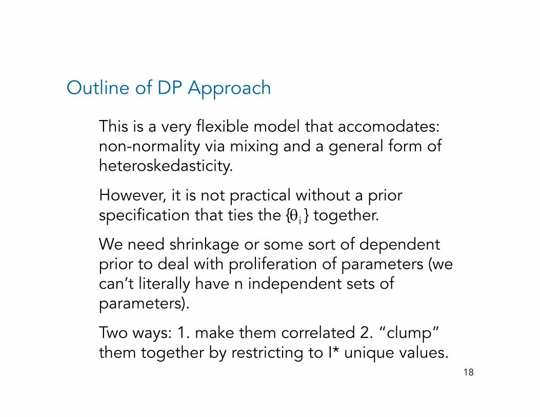
This is a very flexible model that accomodates: This is a very flexible model that accomodates: non-normality via mixing and a general form of heteroskedasticity.
However, it is not practical without a prior specification that ties the {θi } together.
We need shrinkage or some sort of dependent prior to deal with proliferation of parameters (we can’t literally have n independent sets of can t literally have n independent sets of parameters).
Two ways: 1. make them correlated 2. “clump”
18
y pthem together by restricting to I* unique values.
Outline of DP Approach
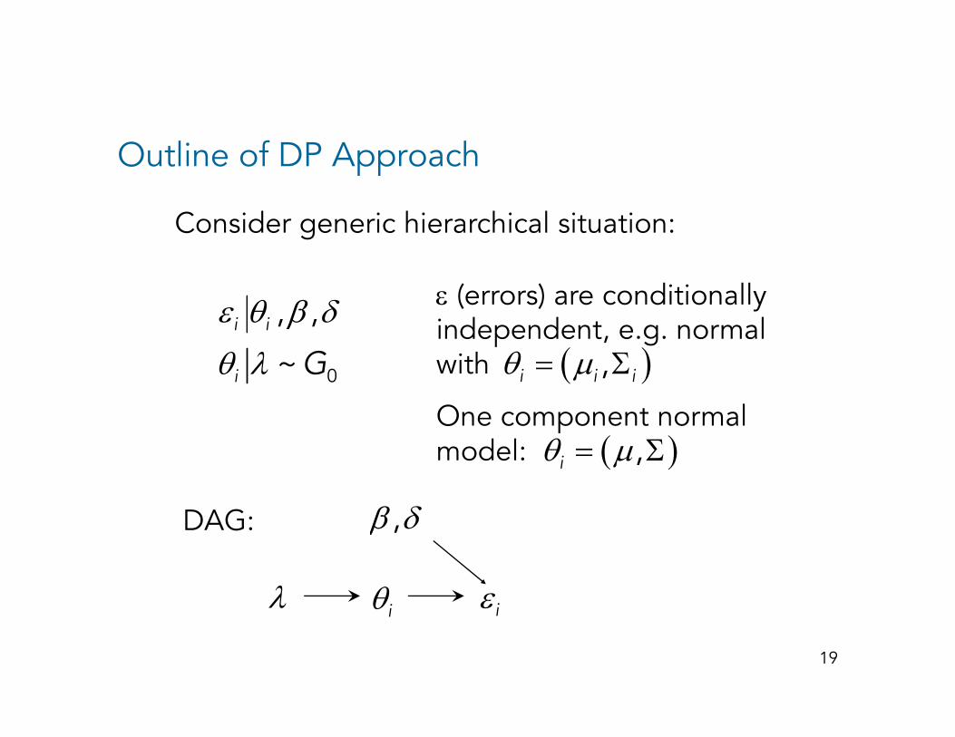
Consider generic hierarchical situation:Consider generic hierarchical situation:
ε θ β δ, ,i iε (errors) are conditionally i d d t l ε θ β δ
θ λ 0
, ,
~i i
i Gindependent, e.g. normal with
One component normal
( )θ μ= Σ,i i i
One component normal model: ( )θ μ= Σ,i
β δDAG:
λ θ ε
β δ,
19
λ θi εi

DP prior
Add another layer to hierarchy – DP prior for thetaAdd another layer to hierarchy DP prior for theta
DAG:
λ θ
β δ,
G
α
G is a Dirichlet Process – a distribution over other
λ θi εiG
distributions. Each draw of G is a Dirichlet Distribution. G is centered on with tightness parameter α
0G
20
parameter α
DPM
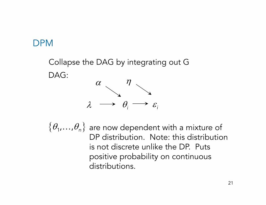
Collapse the DAG by integrating out GCollapse the DAG by integrating out G
DAG:ηα
θi εiλ
{ }θ θ…1, , n are now dependent with a mixture of DP distribution. Note: this distribution is not discrete unlike the DP. Puts positive probability on continuous distributions
21
distributions.

DPM: Drawing from Posterior
Basis for a Gibbs Sampler:Basis for a Gibbs Sampler:
θ ε θ θ ε θ− −=, ,j j j j j
Why? Conditional Independence!
This is a simple update:
There are “n” models for each of the other θ jvalues of theta and the base prior. This is very much like mixture of normals draw of indicators.
j
22
DPM: Drawing from Posterior
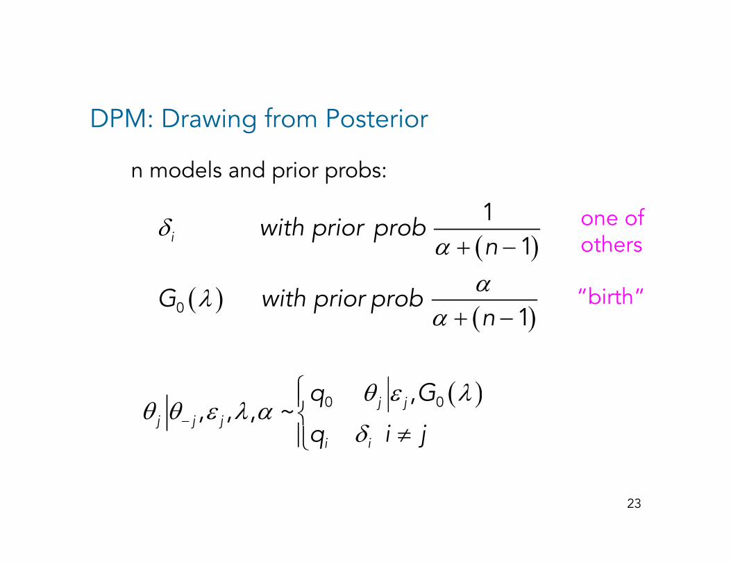
n models and prior probs:n models and prior probs:
( )δ
α +1
1i with prior probn
one of others( )
( )( )
ααλ
α
+ −
+0
1
1
n
G with prior probn
“birth”
others
( )α + −1n
( )θ λ⎧⎪q G ( )θ ε λθ θ ε λ α
δ−
⎧⎪⎨
≠⎪⎩
0 0,, , , ~ j j
j j j
i i
q G
q i j
23

DPM: Drawing from Posterior
( ) ( ) ( ) ( )∫ d( ) ( ) ( ) ( )
( ) ( )
ε ε θ θ λ θ
αε θ θ λ θ
= = ×
= ×
∫
∫
0 0 0j j j j jq p M p p d p M
p G d( ) ( ) ( )
( ) ( )
ε θ θ λ θα
ε ε θ
= ×+ −
= = ×
∫ 0 11
j j j jp G dn
q p M p( ) ( ) ( )ε ε θ
α= = ×
+ −1i i j j iq p M pn
Note: q need to be normalized! Conjugate priors can help to compute q0.
24
Assessing the DP prior
Two Aspects of Prior:p
α-- influences the number of unique values of θ
G λ govern distribution of proposed values G0, λ -- govern distribution of proposed values of θ
e ge.g.
I can approximate a distribution with a large number of “small” normal components or a psmaller number of “big” components.
25

Assessing the DP prior: choice of α
There is a relationship between α and the number pof distinct theta values (viz number of normal components). Antoniak (74) gives this from MDP.
( ) ( )( )ααα
Γ= =
Γ +* ( )Pr k k
nI k Sn
S are “Stirling numbers of First Kind.” Note: S cannot be computed using standard recurrence
l h f 0 h flrelationship for n > 150 without overflow!
( )( )
( )( )γ −Γ+
1( ) lnkk
n
nS n
k26
( )( )( )γ
Γn k

Assessing the DP prior: choice of α
1.0
alpha= 0.001
0
alpha= 0.5
.20.
40.
60.
8
.05
0.10
0.15
0.2
0 10 20 30 40 50
0.0
0
Num Unique
0 10 20 30 40 50
0.00
0
Num UniqueFor N 500
.10
0.15
alpha= 1
40.
06
alpha= 5N=500
0.00
0.05
0
0.00
0.02
0.04
27
0 10 20 30 40 50
Num Unique
0 10 20 30 40 50
Num Unique

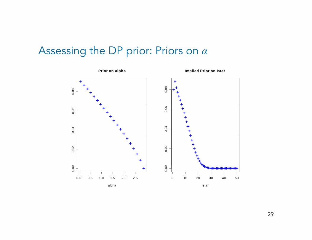
Assessing the DP prior: Priors on α
Fixing may not be reasonable. Prior on number of g yunique theta may be too tight.
“Solution:” put a prior on alpha.p p p
Assess prior by examining the priori distribution of number of unique theta.
( ) ( ) ( )α α α= ∫* *p I p I p d
( ) ( )( )
φα ααα α
⎛ ⎞−∝ −⎜ ⎟−⎝ ⎠
1p
28
( )⎝ ⎠
Assessing the DP prior: Priors on αPrior on alpha Implied Prior on Istar
0.08 0.
08
0.04
0.06
0.04
0.06
00.
02
00.
02
0.0 0.5 1.0 1.5 2.0 2.5
0.00
alpha
0 10 20 30 40 50
0.00
Istar
29

Assessing the DP prior: Choice of λ
( ) ( ) ( ) αε ε θ θ λ θ= = ×∫q p M p G d( ) ( ) ( ) ( )ε ε θ θ λ θ
α= = ×
+ −∫0 0 0 1j j j j jq p M p G dn
Both α and λ determine the probability of a “birth ” Both α and λ determine the probability of a birth.
Intuition:
1. Very diffuse settings of λ reduce model prob.
2. Tight priors centered away from y will also d d l breduce model prob.
Must choose reasonable values. Shouldn’t be very sensitive to this choice
30
sensitive to this choice.

Assessing the DP prior: Choice of λ
( ) ( )μ μ υ− Σ Σ1: ~ ; ~G N a IW V( ) ( )μ μ υΣ Σ0 : , ; ,G N a IW V
Choice of λ made easier if we center and scale both Choice of λ made easier if we center and scale both y and x by the std deviation. Then we know much of mass ε distribution should lie in [-2,2] x [-2,2].
Set μ= =2 and 0V vI
We need assess υ, v, a with the goal of spreading components across the support of the errors.
31
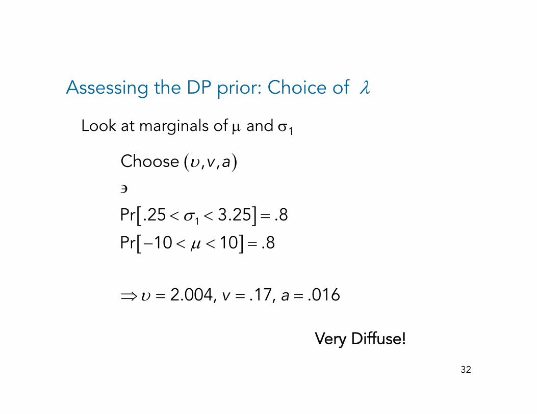
Assessing the DP prior: Choice of λ
Look at marginals of μ and σ1 Look at marginals of μ and σ1
( )υChoose , ,v a
[ ]σ∋
< < =1Pr .25 3.25 .8
[ ]μ− < < =Pr 10 10 .8
υ⇒ = = =2.004, .17, .016v a
Very Diffuse!
32
Very Diffuse!
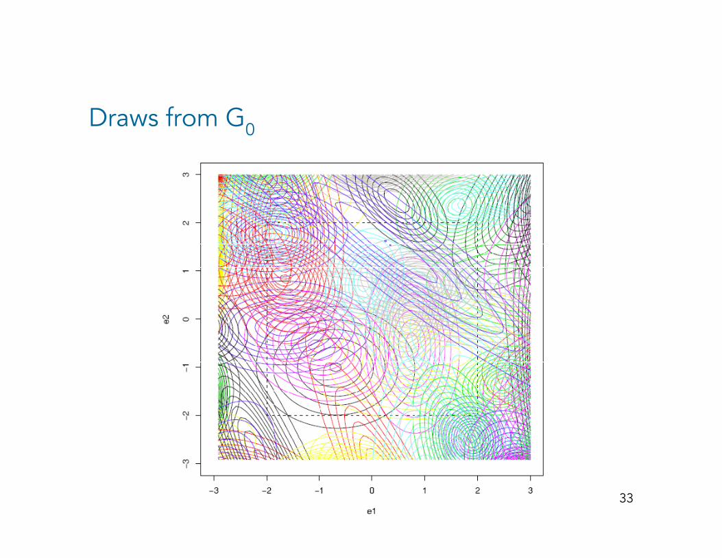
Draws from G0
33
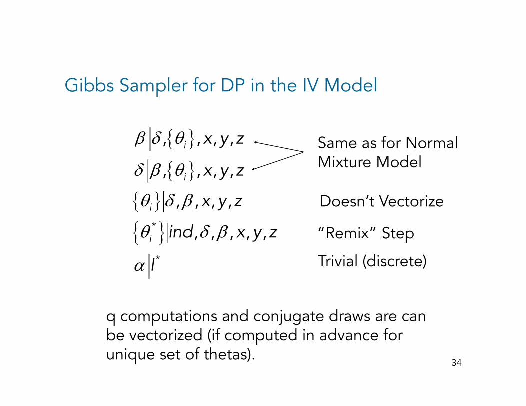
Gibbs Sampler for DP in the IV Model
{ }{ }
β δ θ
δ β θ
, , , ,
, , , ,
i
i
x y z
x y z
Same as for Normal Mixture Model{ }
{ }{ }
β
θ δ β
θ δ β*
, , , ,
, , , ,i
i
y
x y z
i d “R i ” St
Doesn’t Vectorize
{ }θ δ β
α *
, , , , ,i ind x y z
I
“Remix” Step
Trivial (discrete)
q computations and conjugate draws are can b t i d (if t d i d f
34
be vectorized (if computed in advance for unique set of thetas).

Sampling Experiments
1 How well do DP models accommodate 1. How well do DP models accommodate departures to normality?
2 How useful are the DP Bayes results for those 2. How useful are the DP Bayes results for those interested in “standard” inferences such as confidence intervals?
3. How do conditions of many instruments or weak instruments affect performance?
35
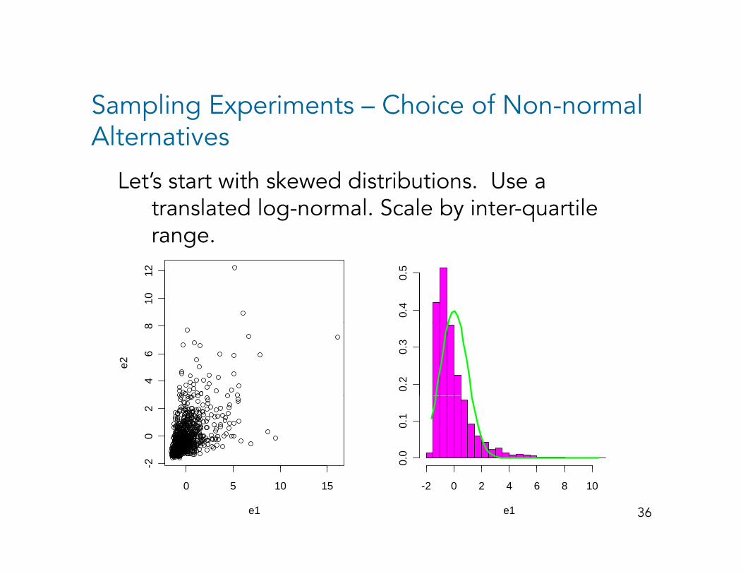
Sampling Experiments Choice of Non normal Sampling Experiments – Choice of Non-normal Alternatives
Let’s start with skewed distributions Use a Let s start with skewed distributions. Use a translated log-normal. Scale by inter-quartile range.
1012
0.4
0.5
46
8
e2
0.2
0.3
-20
2
0.0
0.1
36
0 5 10 15
e1 e1
-2 0 2 4 6 8 10
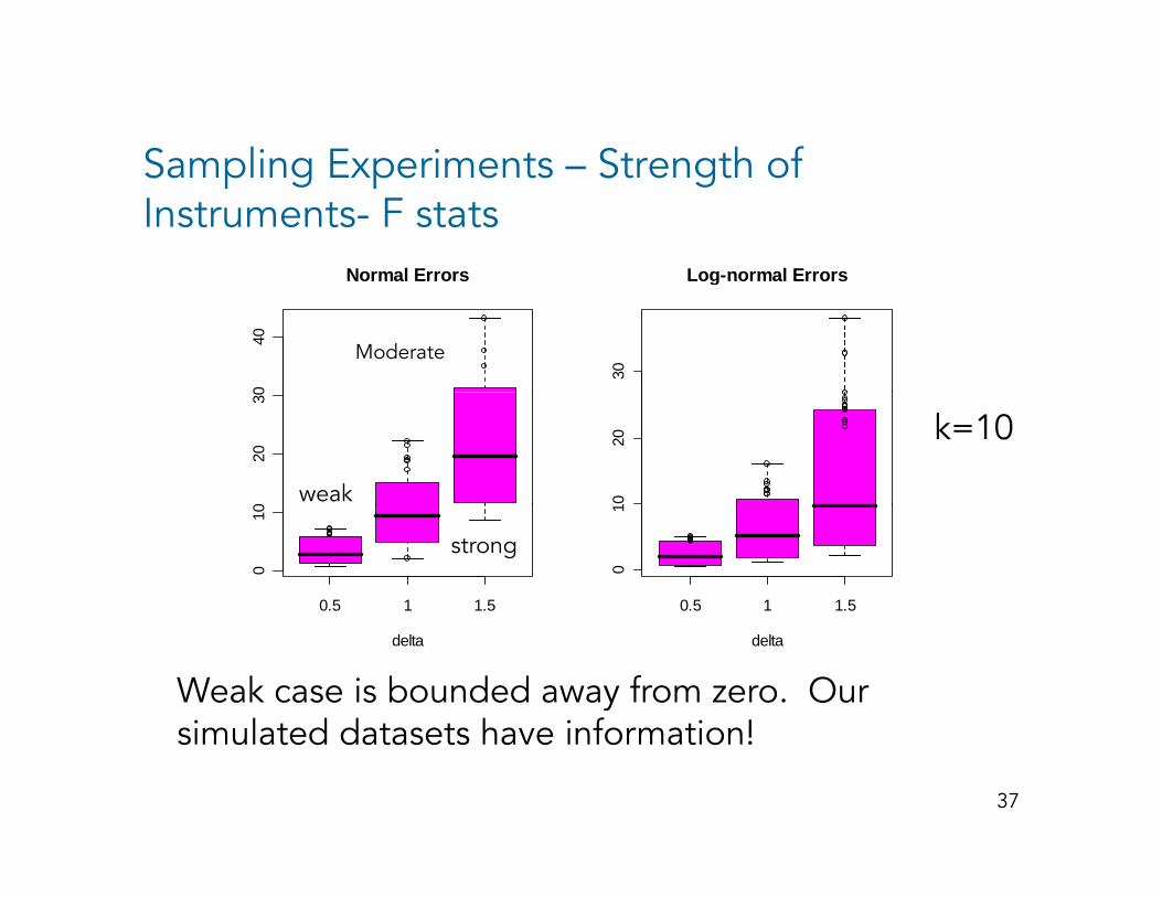
Sampling Experiments Strength of Sampling Experiments – Strength of Instruments- F stats
Normal Errors Log-normal Errors0
40Normal Errors
30
Log normal Errors
Moderate
020
30
020
weak
k=10
0.5 1 1.5
010
0.5 1 1.50
1
strong
delta delta
Weak case is bounded away from zero. Our simulated datasets have information!
37
simulated datasets have information!
Sampling Experiments- Alternative Procedures
Classical Econometrician: “We are interested in Classical Econometrician: We are interested in inference. We are not interested in a better point estimator.”
Standard asymptotics for various K-class estimators
“Many” instruments asymptotics (bound F as k, N Many instruments asymptotics (bound F as k, N increase)
“Weak” instrument asymptotics (bound F and fix k as y pN increases) Kleibergen (K), Modified Kleibergen (J), and Conditional Likelihood Ratio(CLR) (Andrews et al 06)
38
(Andrews et al 06).

Sampling Experiments Coverage of “95%” Sampling Experiments- Coverage of 95% Intervals
N=100; based on 400 reps
error dist BayesDP TSLS-STD Fuller-Many CLRweak
Normal 0.83 0.75 0.93 0.92L N l 0 91 0 69 0 92 0 96LogNormal 0.91 0.69 0.92 0.96
strongNormal 0.92 0.92 0.95 0.94LogNormal 0.96 0.90 0.96 0.95
7% (normal) | 42 % (log-normal)
39
7% (normal) | 42 % (log-normal) are infinite length

Bayes Vs CLR (Andrews 06) Bayes Vs. CLR (Andrews 06)
5040 Weak
I t t
30
sim
#
Instruments Log-Normal
Errors
20
s
010
40-4 -2 0 2 4
0
interval

Bayes Vs Fuller-ManyBayes Vs. Fuller Many
50
Weak I t t
40
Instruments Log-Normal
Errors
30
sim
#
020
010
41
-4 -2 0 2 4
interval
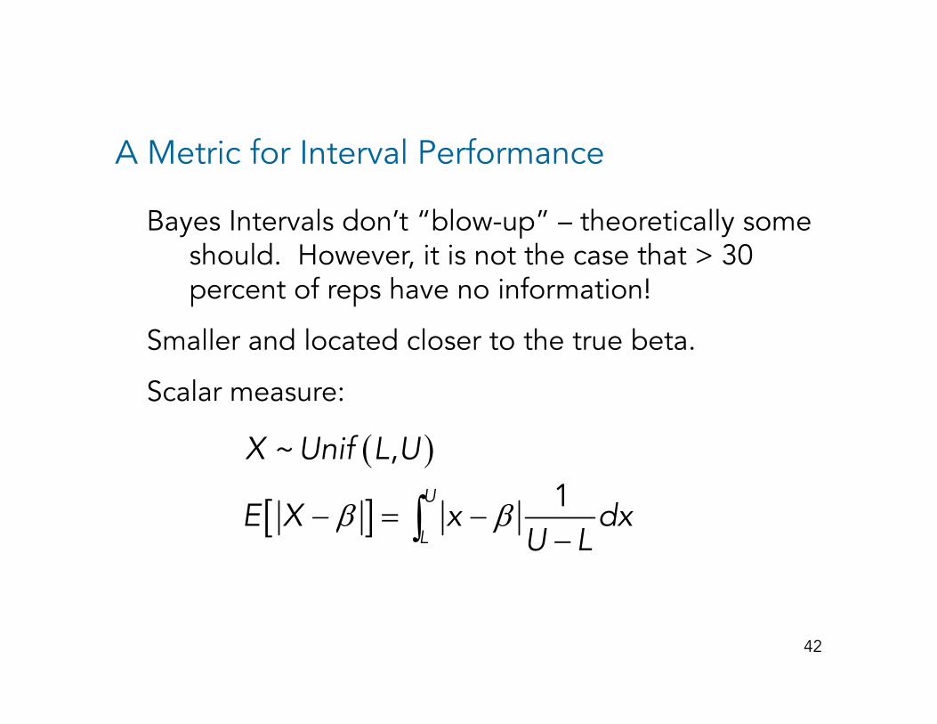
A Metric for Interval Performance
Bayes Intervals don’t “blow-up” – theoretically some Bayes Intervals don t blow up theoretically some should. However, it is not the case that > 30 percent of reps have no information!
Smaller and located closer to the true beta.
Scalar measure:
( )
[ ] ∫
~ ,1U
X Unif L U
[ ]β β− = −−∫1U
LE X x dx
U L
42
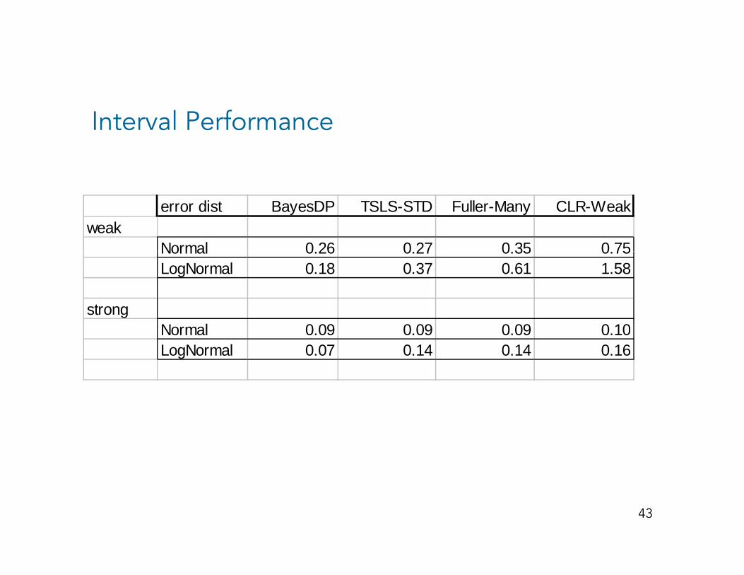
Interval Performance
error dist BayesDP TSLS-STD Fuller-Many CLR-Weakweak
Normal 0 26 0 27 0 35 0 75Normal 0.26 0.27 0.35 0.75LogNormal 0.18 0.37 0.61 1.58
strongN l 0 09 0 09 0 09 0 10Normal 0.09 0.09 0.09 0.10LogNormal 0.07 0.14 0.14 0.16
43
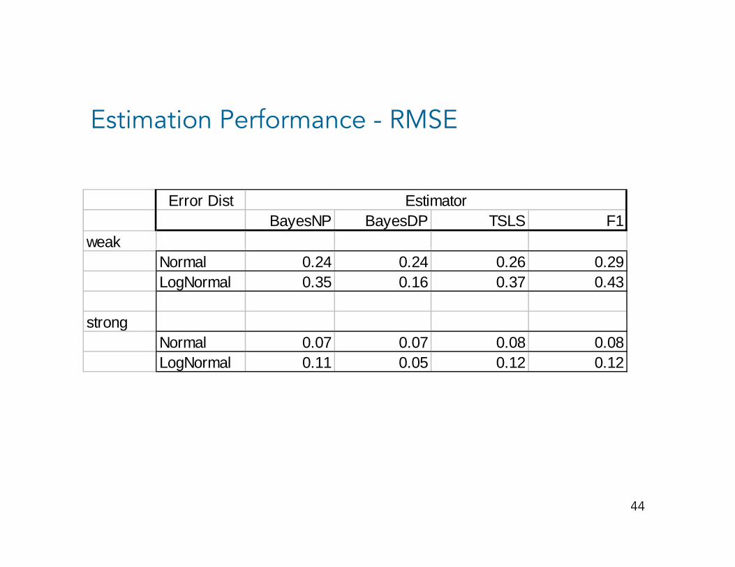
Estimation Performance - RMSE
Error DistBayesNP BayesDP TSLS F1
weak
Estimator
Normal 0.24 0.24 0.26 0.29LogNormal 0.35 0.16 0.37 0.43
strongstrongNormal 0.07 0.07 0.08 0.08LogNormal 0.11 0.05 0.12 0.12
44
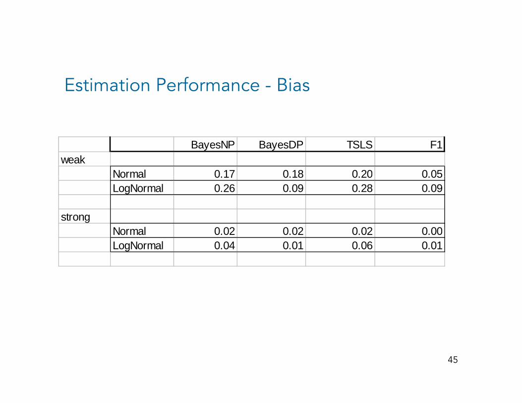
Estimation Performance - Bias
BayesNP BayesDP TSLS F1weak
Normal 0 17 0 18 0 20 0 05Normal 0.17 0.18 0.20 0.05LogNormal 0.26 0.09 0.28 0.09
strongN l 0 02 0 02 0 02 0 00Normal 0.02 0.02 0.02 0.00LogNormal 0.04 0.01 0.06 0.01
45

An Example: Card Data
y is log wage. y is log wage.
x education (yrs)
z is proximity to 2 and 4 year collegesz is proximity to 2 and 4 year colleges
N=3010.
Evidence from standard models is a negative correlation between errors (contrary to the old ability omitted variable interpretation).omitted variable interpretation).
46
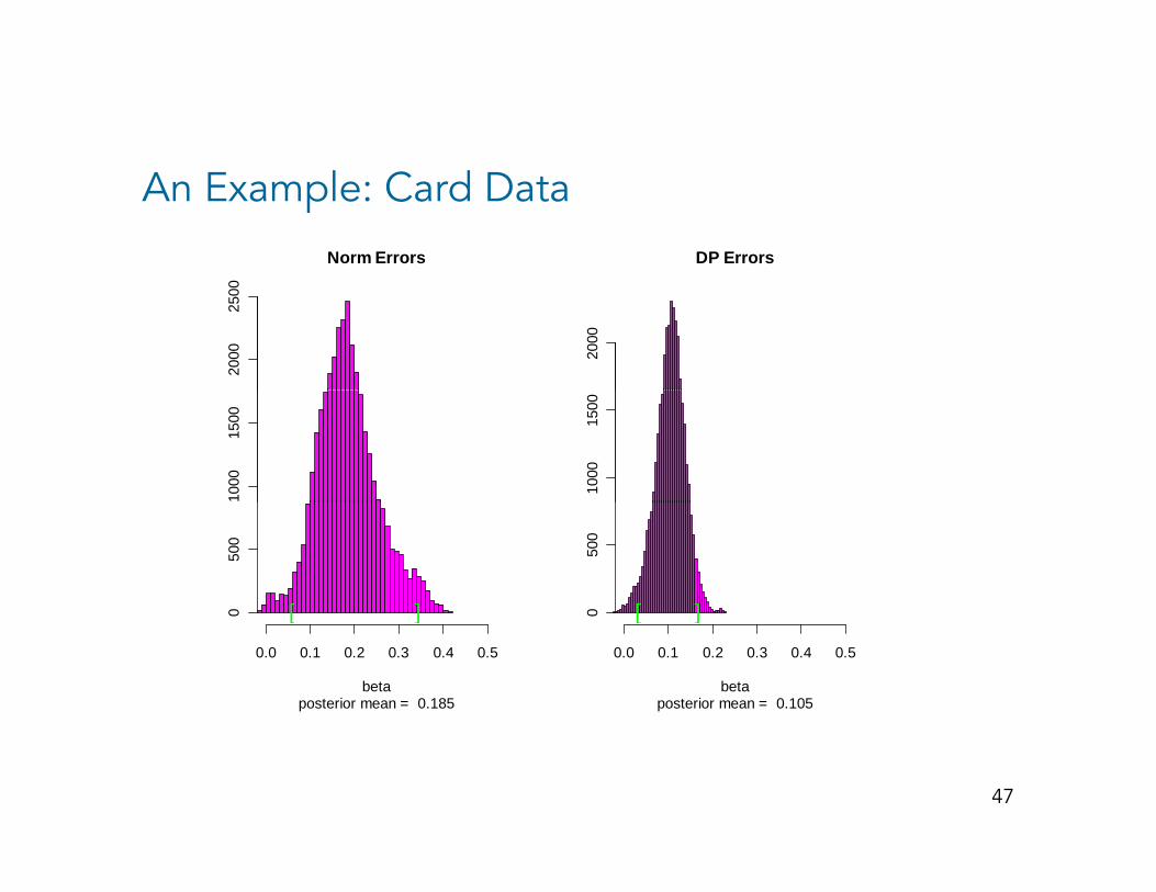
An Example: Card Data
Norm Errors DP Errors20
0025
00
2000
1000
1500
1000
1500
050
0
[ ] 050
0[ ]
posterior mean = 0.185beta
0.0 0.1 0.2 0.3 0.4 0.5
0 [ ]
posterior mean = 0.105beta
0.0 0.1 0.2 0.3 0.4 0.5
0 [ ]
47
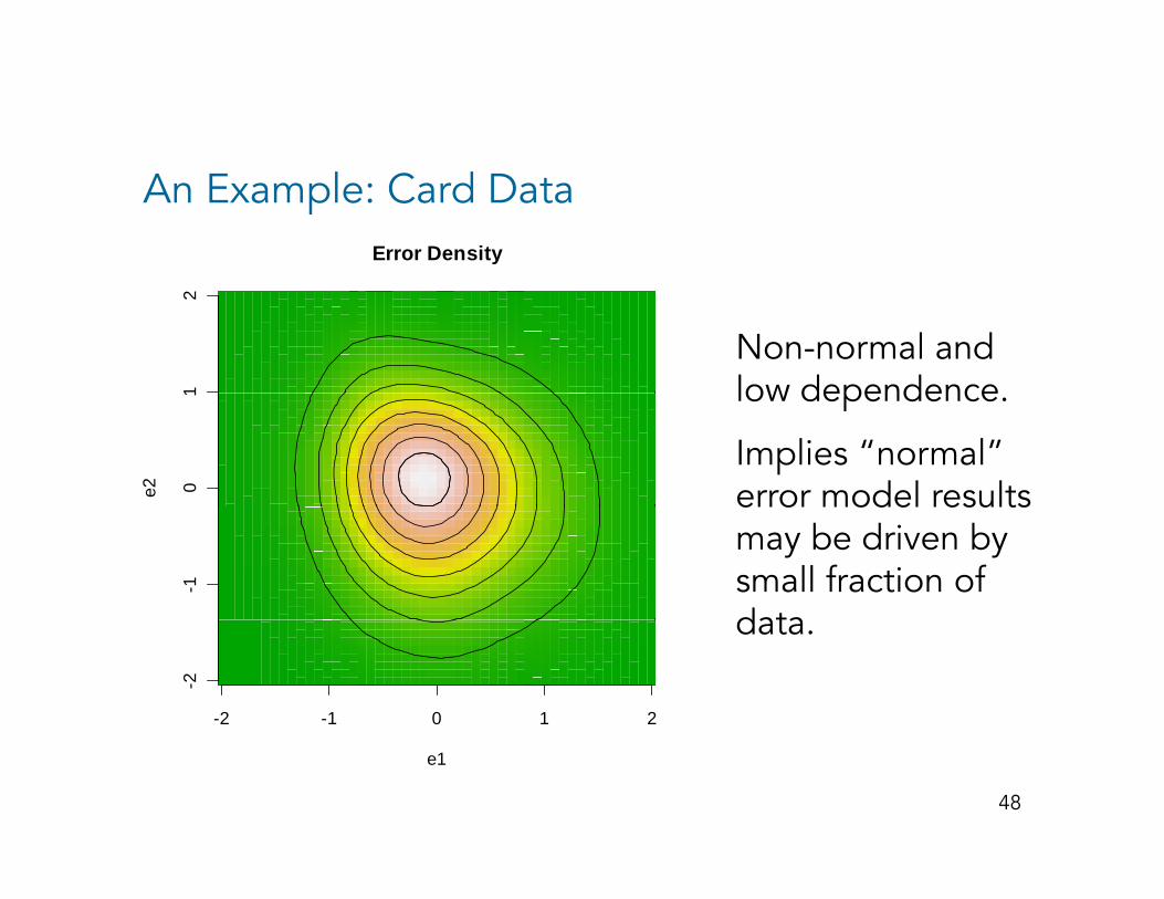
An Example: Card Data Error Density
12
Non-normal and low dependence
01
e2
low dependence.
Implies “normal” error model results
-1
error model results may be driven by small fraction of data
-2 -1 0 1 2
-2
data.
48
e1
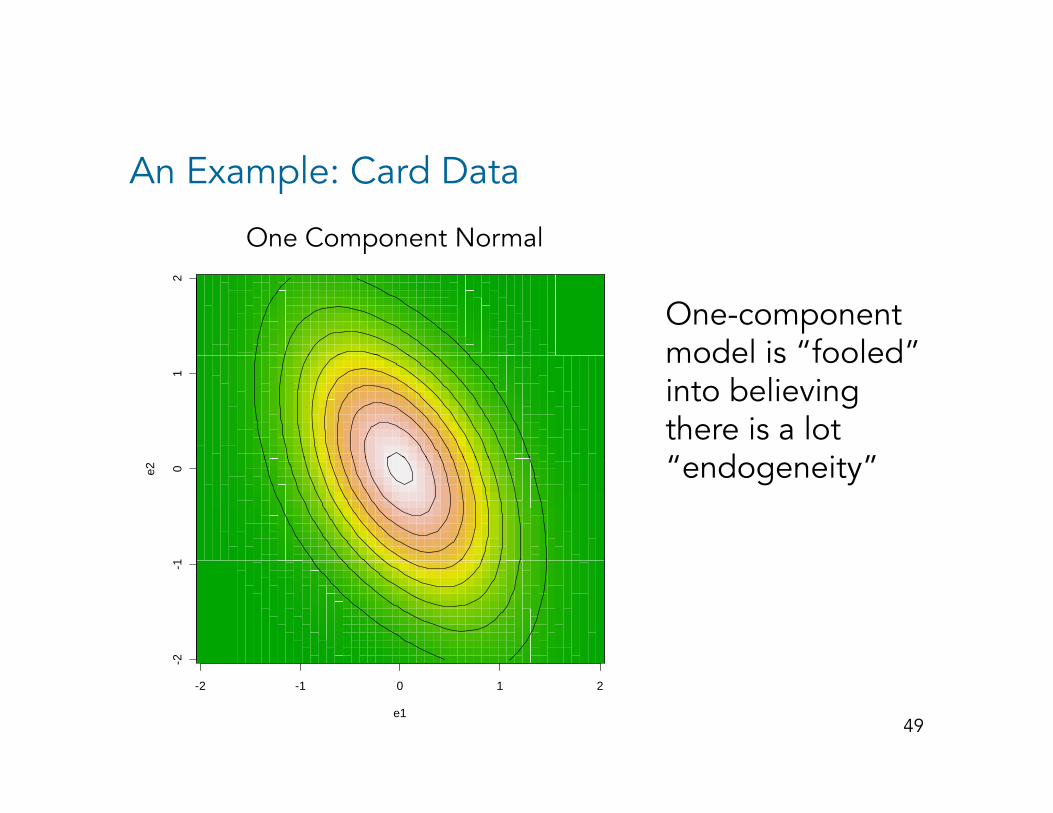
An Example: Card Data
One Component Normal
One-component model is “fooled”
2
p
model is fooled into believing there is a lot “ d i ”
1
“endogeneity”0e2
-2-1
49
-2 -1 0 1 2
-
e1
Summary Bayes DP IV
BayesDP IV works well under the rules of the BayesDP IV works well under the rules of the classical instruments literature game.
BayesDP strictly dominates BayesNPBayesDP strictly dominates BayesNP
Do you want much shorter intervals (more efficient use of sample information) at the expense of use of sample information) at the expense of somewhat lower coverage in very weak instrument case?
50

“Plausibly Exogenous” Instruments
Many IV analyses use instruments that are can be Many IV analyses use instruments that are can be viewed as “approximately” exogenous but that we might argue are not “strictly” exogeneous –
h l l i i i th k t e.g. wholesale prices, prices in other markets, other characteristics …
Yet these analyses impose strict exogeneity in Yet these analyses impose strict exogeneity in estimation. Careful workers use other informal methods for assessing exogeneity such as
b blregressing instruments on observables …
Can we help?
51
“Plausibly Exogenous” Instruments
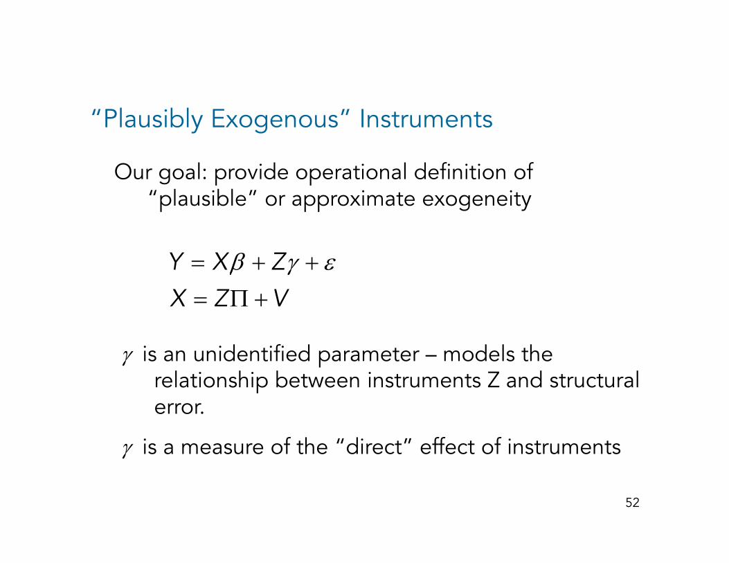
Our goal: provide operational definition of Our goal: provide operational definition of “plausible” or approximate exogeneity
β γ ε= + += Π +
Y X ZX Z V
γ is an unidentified parameter – models the relationship between instruments Z and structural perror.
γ is a measure of the “direct” effect of instruments
52
“Plausibly Exogenous” Instruments
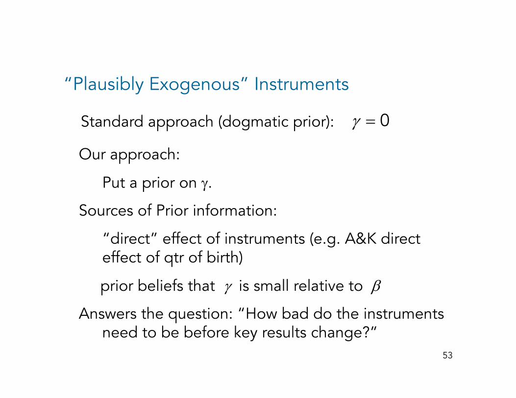
Standard approach (dogmatic prior): γ = 0Standard approach (dogmatic prior): γ 0
Our approach:
Put a prior on γ.
Sources of Prior information:
“direct” effect of instruments (e.g. A&K direct effect of qtr of birth)
prior beliefs that γ is small relative to β
Answers the question: “How bad do the instruments
53
need to be before key results change?”
“Plausibly Exogenous” Instruments
Given some prior information on γ how should we Given some prior information on γ, how should we conduct inference?
Full Bayes (using straightforward extensions of what y ( g gwe have done for strict exogeneity case.
Approximate Bayes:pp
prior-weighted frequentist intervals
intervals constructed via a “local” form of intervals constructed via a local form of asymptotic experiment
Details: Conley, Hansen, Rossi, “Plausibly
54
y, , , yExogenous” SSRN

“Plausibly Exogenous” Examples
Aggregate Share Model for Margarine Demand
( ) ( )β λ γ= + + +log logshare retail price X Z u
gg g g(inspired by Chintagunta, Dube, Goh, 2003)
( ) ( )β λ γ= + + +log logshare retail price X Z u
Wholesale price is “plausibly exogeneous” driven p pmore by cost shocks then manufacturer-sponsored “demand” shocks.
P d ff f h l l l h Prior: direct effects of wholesale price less than price elasticity,
( )γ β δ β2 2~ 0,N
55
( )

“Plausibly Exogenous” Examples
Small Sample: 117117
intervals are insensitive to a β insensitive to a large range of δ
values
β
56δ

“Plausibly Exogenous” Examples
Angrist and Krueger (1991)
( ) ( )β λ γ= + + +log logwage school X Z u
g g
I t t t f bi thInstruments: quarter of birth
Controls: year of birth/state dummies
Bound, Jaeger and Baker argue Q of B is not exogeneous and that direct effect could be of the order of 1 per cent This motivates our the order of 1 per cent. This motivates our choice of prior: ( )γ σ =2 2~ 0, (.005)N
57
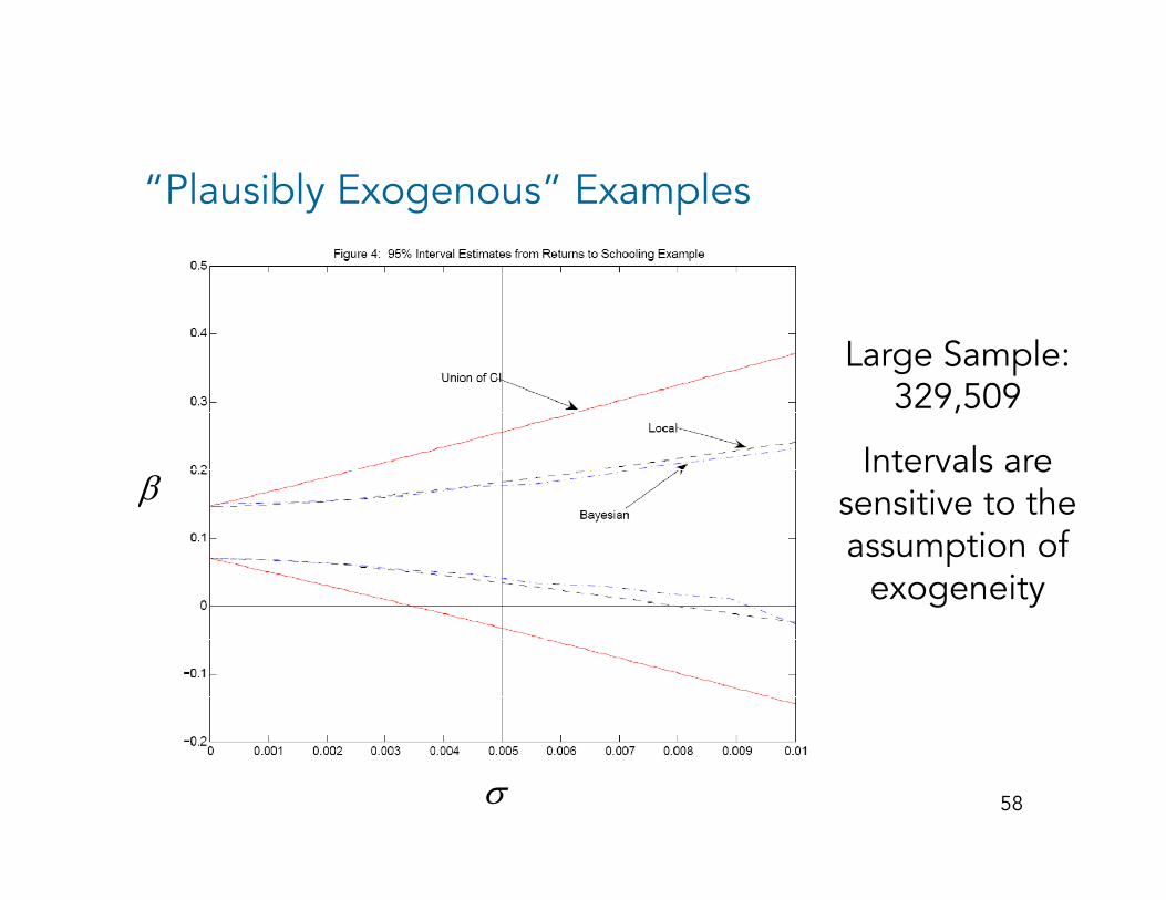
“Plausibly Exogenous” Examples
Large Sample: 329 509329,509
Intervals are sensitive to the β sensitive to the assumption of
exogeneity
β
58σ

Conclusions
A “true” Bayesian IV approach is possible Works A true Bayesian IV approach is possible. Works well relative to “state of the art” frequentist methods
Prior information is important and prior sensitivity analysis is an excellent way to measure sample i f i information
59