bayesian linear mixed models using stan: a tutorial for...

BAYESIAN LINEAR MIXED MODELS: A TUTORIAL 1

Bayesian linear mixed models using Stan: A tutorial forpsychologists, linguists, and cognitive scientists

Tanner SorensenUniversity of Potsdam, Potsdam, Germany

Sven HohensteinUniversity of Potsdam, Potsdam, Germany

Shravan VasishthUniversity of Potsdam, Potsdam, Germany, and

School of Mathematics and Statistics, University of Sheffield, Sheffield, UK

August 10, 2015

Abstract

With the arrival of the R packages nlme and lme4, linear mixed models

(LMMs) have come to be widely used in experimentally-driven areas like psy-

chology, linguistics, and cognitive science. This tutorial provides a practical

introduction to fitting LMMs in a Bayesian framework using the probabilis-

tic programming language Stan. We choose Stan (rather than WinBUGS

or JAGS) because it provides an elegant and scalable framework for fitting

models in most of the standard applications of LMMs. We ease the reader

into fitting increasingly complex LMMs, first using a two-condition repeated

measures self-paced reading study, followed by a more complex 2×2 repeated

measures factorial design that can be generalized to much more complex de-

signs.

Keywords: Bayesian data analysis, linear mixed models, Stan

Introduction

Linear mixed models, or hierarchical/multilevel linear models, have become the main

workhorse of experimental research in psychology, linguistics, and cognitive science, where

repeated measures designs are the norm. Within the programming environment R (R De-

velopment Core Team, 2006), the nlme package (Pinheiro & Bates, 2000) and its successor,

lme4 (Bates, Maechler, Bolker, & Walker, 2014) have revolutionized the use of linear mixed

models (LMMs) due to their simplicity and speed: one can fit fairly complicated models

relatively quickly, often with a single line of code. A great advantage of LMMs over tra-

ditional approaches such as repeated measures ANOVA and paired t-tests is that there is

no need to aggregate over subjects and items to compute two sets of F-scores (or several

t-scores) separately; a single model can take all sources of variance into account simultane-

ously. Furthermore, comparisons between conditions can easily be implemented in a single

model through appropriate contrast coding.

Other important developments related to LMMs have been unfolding in computa-

tional statistics. Specifically, probabilistic programming languages like WinBUGS (Lunn,

Thomas, Best, & Spiegelhalter, 2000), JAGS (Plummer, 2012) and Stan (Stan Develop-

ment Team, 2014), among others, have made it possible to fit Bayesian LMMs quite easily.

However, one prerequisite for using these programming languages is that some background

statistical knowledge is needed before one can define the model. This difficulty is well-

known; for example, Spiegelhalter, Abrams, and Myles (2004, 4) write: “Bayesian statistics

has a (largely deserved) reputation for being mathematically challenging and difficult to

put into practice. . . ”.

The purpose of this paper is to facilitate a first encounter with model specification in

one of these programming languages, Stan. The tutorial is aimed primarily at psychologists,

linguists, and cognitive scientists who have used lme4 to fit models to their data, but may

have only a basic knowledge of the underlying LMM machinery. A diagnostic test is that

Please send correspondence to {tanner.sorensen,sven.hohenstein,vasishth}@uni-potsdam.de.


they may not be able to answer some or all of these questions: what is a design matrix; what

is contrast coding; what is a random effects variance-covariance matrix in a linear mixed

model? Our tutorial is not intended for statisticians or psychology researchers who could,

for example, write their own Markov Chain Monte Carlo samplers in R or C++ or the like;

for them, the Stan manual is the optimal starting point. The present tutorial attempts

to ease the beginner into their first steps towards fitting Bayesian linear mixed models.

More detailed presentations about linear mixed models are available in several textbooks;

references are provided at the end of this tutorial.

We have chosen Stan as the programming language of choice (over JAGS and Win-

BUGS) because it is possible to fit arbitrarily complex models with Stan. For example, it is

possible (if time consuming) to fit a model with 14 fixed effects predictors and two crossed

random effects by subject and item, each involving a 14 × 14 variance-covariance matrix

(Bates, Kliegl, Vasishth, & Baayen, 2015); as far as we are aware, such models cannot, as

far as we know, be fit in JAGS or WinBUGS.1

In this tutorial, we take it as a given that the reader is interested in learning how to fit

Bayesian linear mixed models. The tutorial is structured as follows. After a short introduc-

tion to Bayesian modeling, we begin by successively building up increasingly complex LMMs

using the data-set reported by Gibson and Wu (2013), which has a simple two-condition

design. At each step, we explain the structure of the model. The next section takes up

inference for this two-condition design. Then we demonstrate how one can fit models using

the matrix formulation of the design.

This paper was written using a literate programming tool, knitr (Xie, 2013); this

integrates documentation for the accompanying code with the paper. The knitr file that

generated this paper, as well as all the code and data used in this tutorial, can be downloaded

from our website:

http://www.ling.uni-potsdam.de/~vasishth/statistics/BayesLMMs.html

In addition, the source code for the paper, all R code, and data are available on github at:1Whether it makes sense in general to fit such a complex model is a different issue; see Gelman et al.

(2014), and Bates et al. (2015) for recent discussion.


https://github.com/vasishth/BayesLMMTutorial

We start with the two-condition repeated measures data-set (Gibson &Wu, 2013) as a

concrete running example. This simple example serves as a starter kit for fitting commonly

used LMMs in the Bayesian setting. We assume that the reader has the relevant software

installed; specifically, rstan in R. For detailed instructions, see

https://github.com/stan-dev/rstan/wiki/RStan-Getting-Started

Bayesian modeling

Bayesian modeling has two major advantages over frequentist analysis with linear

mixed models. First, information based on preceding results can be incoportated using dif-

ferent priors. Second, complex models with a large number of random variance components

can be fit. In the following, we will provide a short introduction to Bayesian statistics.

Bayesian modeling is based on Bayes’ Theorem. It can be seen as a way of understand-

ing how the probability that a hypothesis is true is affected by new data. In mathematical

notation,

P (H|D) = P (D|H)P (H)P (D) ,

H is the hypothesis we are interested in, and D represents new data. Since D is fixed

for a given data-set, the theorem can be rephrased as,

P (H|D) ∝ P (D|H)P (H).

The posterior probability that the hypothesis is true given new data, P (H|D), is

proportional to the product of the likelihood of the new data given the hypothesis, P (D|H),

and the prior probability of the hypothesis, P (H).

For the purposes of this paper, the goal of a Bayesian analysis is simply to derive the

posterior distribution of each parameter of interest, given some data and prior beliefs about

the distributions of the parameters. The following example illustrates how the posterior


0 50 100 150

0.00

0.01

0.02

0.03

0.04

0.05

0.06

x

Den

sity

PriorLikelihoodPosterior

0 50 100 150

0.00

0.01

0.02

0.03

0.04

0.05

0.06

xD

ensi

ty

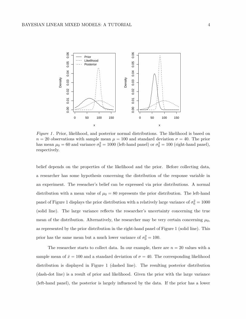
Figure 1 . Prior, likelihood, and posterior normal distributions. The likelihood is based onn = 20 observations with sample mean µ = 100 and standard deviation σ = 40. The priorhas mean µ0 = 60 and variance σ2

0 = 1000 (left-hand panel) or σ20 = 100 (right-hand panel),

respectively.

belief depends on the properties of the likelihood and the prior. Before collecting data,

a researcher has some hypothesis concerning the distribution of the response variable in

an experiment. The reseacher’s belief can be expressed via prior distributions. A normal

distribution with a mean value of µ0 = 80 represents the prior distribution. The left-hand

panel of Figure 1 displays the prior distribution with a relatively large variance of σ20 = 1000

(solid line). The large variance reflects the researcher’s uncertainty concerning the true

mean of the distribution. Alternatively, the researcher may be very certain concerning µ0,

as represented by the prior distribution in the right-hand panel of Figure 1 (solid line). This

prior has the same mean but a much lower variance of σ20 = 100.

The researcher starts to collect data. In our example, there are n = 20 values with a

sample mean of x̄ = 100 and a standard deviation of σ = 40. The corresponding likelihood

distribution is displayed in Figure 1 (dashed line). The resulting posterior distribution

(dash-dot line) is a result of prior and likelihood. Given the prior with the large variance

(left-hand panel), the posterior is largely influenced by the data. If the prior has a lower


variance (right-hand panel), its influence on the posterior is much stronger resulting is a

stroger shift towards the prior’s mean.

This toy example illustrates the central idea of Bayesian modeling. The prior reflects

our knowledge of past results. In most cases, we will use so-called vague flat priors such that

the posterior distribution is mainly affected by the data. The resulting posterior distribution

allows for calculating credible intervals of true parameter values (see below).

For further explanation of the advantages this approach affords beyond the classical

frequentist approach, the reader is directed to the rich literature relating to a comparison

between Bayesian versus frequentist statistics (such as the provocatively titled paper by

Lavine 1999; and the highly accessible textbook by Kruschke 2014).

The second advantage of Bayesian modeling concerns variance components (random

effects). Fitting a large number of random effects in non-Bayesian settings requires a large

amount of data. Often, the data-set is too small to fit reliable distributions of random effects

(Bates et al., 2015). However, if a researcher is interested in differences between individual

subjects or items (random intercepts and random slopes) or relationships between differences

(correlations between variance components), Bayesian modeling can be used even if there is

not enough data for inferential statistics. The resulting posterior distributions might have

high variance but they still allow for calculating probabilities of true parameter values of

variance components. Note that we do not intend to critisice classical LMMs but highlight

possibilities of Bayesian modeling concerning random effects.

Example 1: A two-condition repeated measures design

This section motivates the LMM with the self-paced reading data-set of Gibson and

Wu (2013). We introduce the data-set, state our modeling goals here, and proceed to build

up increasingly complex LMMs.

The scientific question. Subject and object relative clauses have been widely used

in reading studies to investigate sentence comprehension processes. A subject relative is a

sentence like The senator who interrogated the journalist resigned where a noun (senator)


is modified by a relative clause (who interrogated the journalist), and the modified noun is

the grammatical subject of the relative clause. In an object relative, the noun modified by

the relative clause is the grammatical object of the relative clause (e.g., The senator who

the journalist interrogated resigned). In both cases, the noun that is modified (senator) is

called the head noun.

A typical finding for English is that subject relatives are easier to process than ob-

ject relatives (Just & Carpenter, 1992). Natural languages generally have relative clauses,

and the subject relative advantage has until recently been considered to be true cross-

linguistically. However, Chinese relative clauses apparently represent an interesting counter-

example to this generalization; recent work by Hsiao and Gibson (2003) has suggested that

in Chinese, object relatives are easier to process than subject relatives at a particular point

in the sentence (the head noun of the relative clause). We now present an analysis of a

subsequently published data-set (Gibson & Wu, 2013) that evaluates this claim.

The data. The dependent variable of the experiment of Gibson and Wu (2013)

was the reading time rt of the head noun of the relative clause. This was recorded in two

conditions (subject relative and object relative), with 37 subjects and 15 items, presented in

a standard Latin square design. There were originally 16 items, but one item was removed,

resulting in 37× 15 = 555 data points. However, eight data points from one subject (id 27)

were missing. As a consequence, we have a total of 555 − 8 = 547 data points. The first

few lines from the data frame are shown in Table 1; “o” refers to object relative and “s” to

subject relative.

We build up the Bayesian LMM from a fixed effects simple linear model to a varying

intercepts model and finally to a varying intercepts, varying slopes model (the “maximal

model” of Barr, Levy, Scheepers, and Tily 2013). The result is a probability model that

expresses how the dependent variable, the reading time labeled rt, was generated in the

experiment of Gibson and Wu (2013).

As mentioned above, the goal of Bayesian modeling is to derive the posterior probabil-

ity distribution of the model parameters from a prior probability distribution and a likelihood


row subj item so rt1 1 13 o 15612 1 6 s 9593 1 5 o 5824 1 9 o 2945 1 14 s 4386 1 4 s 286...

......

...547 9 11 o 350

Table 1First six rows, and the last row, of the data-set of Gibson and Wu (2013), as they appearin the data frame.

function. Stan makes it easy to compute this posterior distribution of each parameter of in-

terest. The posterior distribution reflects what we should believe, given the data, regarding

the value of that parameter.

Fixed Effects Model (Simple Linear Model)

We begin by making the working assumption that the dependent variable of reading

time rt on the head noun is approximately log-normally distributed (Rouder, 2005). This

assumes that the logarithm of rt is approximately normally distributed. The logarithm of

the reading times, log rt, has some unknown grand mean β0. The mean of the log-normal

distribution of rt is the sum of β0 and an adjustment β1×so whose magnitude depends on

the categorical predictor so, which has the value −1 when rt is from the subject relative

condition, and 1 when rt is from the object relative condition. One way to write the model

in terms of the logarithm of the reading times is as follows:

log rti = β0 + β1soi + εi (1)

The index i represents the i-th row in the data-frame (in this case, i ∈ {1, . . . , 547});

the term εi represents the error in the i-th row. With the above ±1 contrast coding, β0

represents the grand mean of log rt, regardless of relative clause type. It can be estimated

by simply taking the grand mean of log rt. The parameter β1 is an adjustment to β0 so


that the mean of log rt is β0 + 1β1 when log rt is from the object relative condition, and

β0 − 1β1 when log rt is from the subject relative condition. Notice that 2× β1 will be the

difference in the means between the object and subject relative clause conditions. Together,

β0 and β1 make up the part of the model which characterizes the effect of the experimental

manipulation, relative clause type (so), on the dependent variable rt. We call this a fixed

effects model because we estimate the β parameters, which are unvarying from subject to

subject and from item to item. In R, this would correspond to fitting a simple linear model

using the lm function, with so as predictor and log rt as dependent variable.

The error εi is positive when log rti is greater than the expected value µi = β0 +β1soi

and negative when log rti is less than the expected value µi. Thus, the error is the amount

by which the expected value differs from actually observed value. It is standardly assumed

that the εi are independently and identically distributed as a normal distribution with

mean zero and unknown standard deviation σe. Stan parameterizes the normal distribution

by the mean and standard deviation, and we follow that convention here, by writing the

distribution of ε as N (0, σe) (the standard notation in statistics is in terms of mean and

variance). A consequence of the assumption that the errors are identically distributed is

that the distribution of ε should, at least approximately, have the same shape as the normal

distribution. Independence implies that there should be no correlation between the errors—

this is not the case in the data, since we have multiple measurements from each subject,

and from each item.

Setting up the data. We now fit the fixed effects Model 1. For the following

discussion, please refer to the code in Listings 1 (R code) and 2 (Stan code). First, we

read the Gibson and Wu (2013) data into a data frame rDat in R, and then subset the

critical region (Listing 1, lines 2 and 4). Next, we create a data list stanDat for Stan, which

contains the data (line 7). Stan requires the data to be of type list; this is different from

the lm and lmer functions, which assume that the data are of type data-frame.


1 # read in data:2 rDat <- read.table("gibsonwu2012data.txt", header = TRUE)3 # subset critical region:4 rDat <- subset(rDat, region == "headnoun")5

6 # create data as list for Stan, and fit model:7 stanDat <- list(rt = rDat$rt, so = rDat$type, N = nrow(rDat))8 library(stan)9 fixEfFit <- stan(file = "fixEf.stan", data = stanDat,

10 iter = 2000, chains = 4)11

12 # plot traceplot, excluding warm-up:13 traceplot(fixEfFit, pars = c("beta", "sigma_e"),14 inc_warmup = FALSE)15

16 # examine quantiles of posterior distributions:17 print(fixEfFit, pars = c("beta", "sigma_e"),18 probs = c(0.025, 0.5, 0.975))19

20 # examine quantiles of parameter of interest:21 beta1 <- unlist(extract(fixEfFit, pars = "beta[2]"))22 print(quantile(beta1, probs = c(0.025, 0.5, 0.975)))

Listing 1: Code for the fixed effects Model 1.

1 data {2 int<lower=1> N; //number of data points3 real rt[N]; //reading time4 real<lower=-1,upper=1> so[N]; //predictor5 }6 parameters {7 vector[2] beta; //intercept and slope8 real<lower=0> sigma_e; //error sd9 }

10 model {11 real mu;12 for (i in 1:N){ // likelihood13 mu <- beta[1] + beta[2] * so[i];14 rt[i] ~ lognormal(mu, sigma_e);15 }16 }

Listing 2: Stan code for the fixed effects Model 1.


Defining the model. The next step is to write the Stan model in a text file with

extension .stan. A Stan model consists of several blocks. A block is a set of statements

surrounded by brackets and preceded by the block name. We open up a file fixEf.stan in

a text editor and write down the first block, the data block, which contains the declaration

of the variables in the data object stanDat (Listing 2, lines 1–5). The strings real and

int specify the data type for each variable. A real variable is a real number (R), and an

int variable is an integer (Z). For instance, N is the integer number of data points. The

variables so and rt are arrays of length N whose entries are real. We constrain a variable

to take only a subset of the values allowed by its type (e.g. int or real) by specifying in

brackets lower and upper bounds (e.g. <lower=-1,upper=1>). The variables in the data

block, N, rt, and so, correspond to the values of the list stanDat in R.

Next, we turn to the parameters block, where the parameters are defined (Listing 2,

lines 6–9). These are the parameters for which posterior distributions are of interest. The

fixed effects Model 1 has three parameters: the fixed intercept β0, the fixed slope β1, and

the standard deviation σe of the error. The fixed effects β0 and β1 are in the vector beta

of length two; note that although we called our parameters β0 and β1 in Model 1, in Stan,

these are contained in a vector with indices 1 and 2, so β0 is in beta[1] and β1 in beta[2].

The third parameter, the standard deviation σe of the error (sigma_e), is also defined here,

and is constrained to have lower bound 0 (Listing 2, line 8).

Finally, the model block specifies the prior distribution and the likelihood (Listing 2,

lines 10–15). To understand the Stan syntax, compare the Stan code above to the specifi-

cation of Model 1. The Stan code literally writes out this model. The block begins with a

local variable declaration for mu, which is the mean of rt conditional on whether so is −1

for the subject relative condition or 1 for the object relative condition.

The prior distributions on the parameters beta and sigma_e would ordinarily be de-

clared in the model block. If we don’t declare any prior, it is assumed that they have a

uniform prior distribution. Note that the distribution of sigma_e is truncated at zero be-

cause sigma_e is constrained to be positive (see the declaration real<lower=0> sigma_e;


in the parameters block). So, this means that the error has a uniform prior with lower

bound 0.

In the model block, the for-loop assigns to mu the mean for the log-normal distribution

of rt[i], conditional on the value of the predictor so[i] for relative clause type. The

statement rt[i] ∼ lognormal(mu, sigma_e) means that the logarithm of each value in

the vector rt is normally distributed with mean mu and standard deviation sigma_e. One

could have equally well log-transformed the reading time and assumed a normal distribution

instead of the lognormal.

Running the model. We save the file fixEf.stan which we just wrote and fit the

model in R with the function stan from the package rstan (Listing 1, lines 9 and 10). This

call to the function stan will compile a C++ program which produces samples from the

joint posterior distribution of the fixed intercept β0, the fixed slope β1, and the standard

deviation σe of the error. Here, the function generates four chains of samples, each of which

contains 2000 samples of each parameter. Samples 1 to 1000 are part of the warmup, where

the chains settle into the posterior distribution. We analyze samples 1001 to 2000. The

result is saved to an object fixEfFit of class stanFit.

The warmup samples, also known as the burn-in period, are intended to allow the

MCMC sampling process to converge to the equilibrium distribution, the desired joint

distribution over the variables. This is necessary since the initial values of the parameters

might be very unlikely under the equilibrium distribution and hence bias the result. Once a

chain has converged, the samples remain quite stable. Before the MCMC sampling process,

the number of interations necessary for convergence is unknown. Therefore, all warmup

iterations are discarded.

The number of iterations necessary for convergence to the equilibrium distribution

depends on the number of parameters. The probability to reach convergence increases with

the number of iterations. Hence, we generally recommend using a large number of iterations

although the process might converge after a smaller number of iterations. In the examples

in the present paper, we use 1000 iterations for warmup and another 1000 iterations for


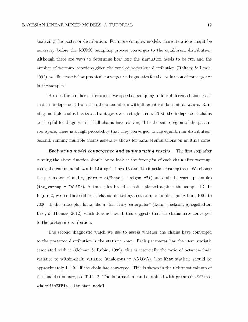
analyzing the posterior distribution. For more complex models, more iterations might be

necessary before the MCMC sampling process converges to the equilibrum distribution.

Although there are ways to determine how long the simulation needs to be run and the

number of warmup iterations given the type of posteriour distribution (Raftery & Lewis,

1992), we illustrate below practical convergence diagnostics for the evaluation of convergence

in the samples.

Besides the number of iterations, we specified sampling in four different chains. Each

chain is independent from the others and starts with different random initial values. Run-

ning multiple chains has two advantages over a single chain. First, the independent chains

are helpful for diagnostics. If all chains have converged to the same region of the param-

eter space, there is a high probability that they converged to the equilibrium distribution.

Second, running multiple chains generally allows for parallel simulations on multiple cores.

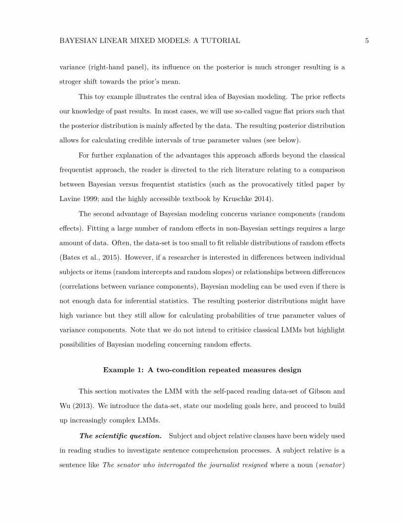
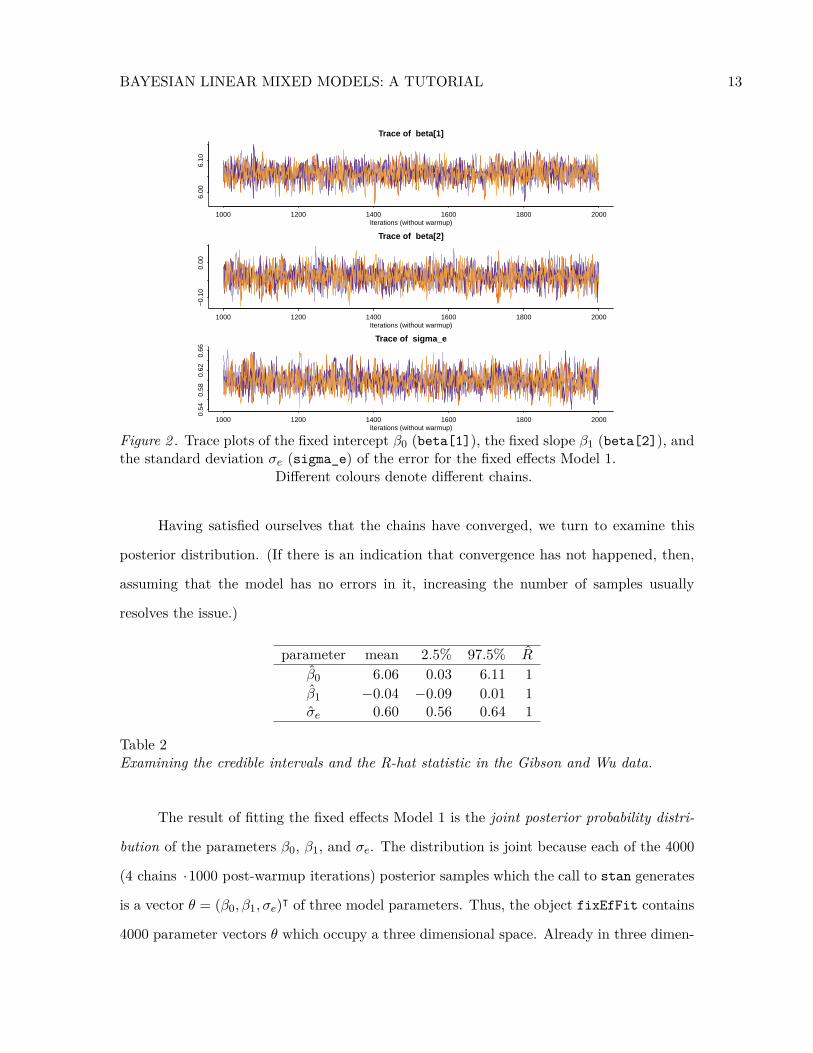
Evaluating model convergence and summarizing results. The first step after

running the above function should be to look at the trace plot of each chain after warmup,

using the command shown in Listing 1, lines 13 and 14 (function traceplot). We choose

the parameters βi and σe (pars = c("beta", "sigma_e")) and omit the warmup samples

(inc_warmup = FALSE)). A trace plot has the chains plotted against the sample ID. In

Figure 2, we see three different chains plotted against sample number going from 1001 to

2000. If the trace plot looks like a “fat, hairy caterpillar” (Lunn, Jackson, Spiegelhalter,

Best, & Thomas, 2012) which does not bend, this suggests that the chains have converged

to the posterior distribution.

The second diagnostic which we use to assess whether the chains have converged

to the posterior distribution is the statistic Rhat. Each parameter has the Rhat statistic

associated with it (Gelman & Rubin, 1992); this is essentially the ratio of between-chain

variance to within-chain variance (analogous to ANOVA). The Rhat statistic should be

approximately 1± 0.1 if the chain has converged. This is shown in the rightmost column of

the model summary, see Table 2. The information can be otained with print(fixEfFit),

where fixEfFit is the stan.model.


1000 1200 1400 1600 1800 2000

6.00

6.10

Trace of beta[1]

Iterations (without warmup)

1000 1200 1400 1600 1800 2000

−0.

100.

00

Trace of beta[2]


1000 1200 1400 1600 1800 2000

0.54

0.58

0.62

0.66

Trace of sigma_e


Figure 2 . Trace plots of the fixed intercept β0 (beta[1]), the fixed slope β1 (beta[2]), andthe standard deviation σe (sigma_e) of the error for the fixed effects Model 1.

Different colours denote different chains.

Having satisfied ourselves that the chains have converged, we turn to examine this

posterior distribution. (If there is an indication that convergence has not happened, then,

assuming that the model has no errors in it, increasing the number of samples usually

resolves the issue.)

parameter mean 2.5% 97.5% R̂

β̂0 6.06 0.03 6.11 1β̂1 −0.04 −0.09 0.01 1σ̂e 0.60 0.56 0.64 1

Table 2Examining the credible intervals and the R-hat statistic in the Gibson and Wu data.

The result of fitting the fixed effects Model 1 is the joint posterior probability distri-

bution of the parameters β0, β1, and σe. The distribution is joint because each of the 4000

(4 chains ·1000 post-warmup iterations) posterior samples which the call to stan generates

is a vector θ = (β0, β1, σe)ᵀ of three model parameters. Thus, the object fixEfFit contains

4000 parameter vectors θ which occupy a three dimensional space. Already in three dimen-


β0

Den

sity

6.00 6.05 6.10 6.15

02

46

810

14

−0.10 −0.05 0.00 0.05

6.00

6.05

6.10

6.15

β1

β 0

β1

Den

sity

−0.10 −0.05 0.00 0.05

05

1015

0.54 0.58 0.62 0.66

6.00

6.05

6.10

6.15

σe

β 0

0.54 0.58 0.62 0.66

−0.

10−

0.05

0.00

0.05

σe

β 1

σe

Den

sity

0.54 0.58 0.62 0.66

05

1015

20

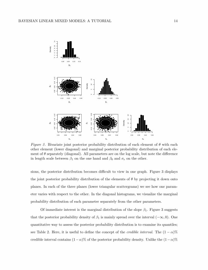
Figure 3 . Bivariate joint posterior probability distribution of each element of θ with eachother element (lower diagonal) and marginal posterior probability distribution of each ele-ment of θ separately (diagonal). All parameters are on the log scale, but note the differencein length scale between β1 on the one hand and β0 and σe on the other.

sions, the posterior distribution becomes difficult to view in one graph. Figure 3 displays

the joint posterior probability distribution of the elements of θ by projecting it down onto

planes. In each of the three planes (lower triangular scattergrams) we see how one param-

eter varies with respect to the other. In the diagonal histograms, we visualize the marginal

probability distribution of each parameter separately from the other parameters.

Of immediate interest is the marginal distribution of the slope β1. Figure 3 suggests

that the posterior probability density of β1 is mainly spread over the interval (−∞, 0). One

quantitative way to assess the posterior probability distribution is to examine its quantiles;

see Table 2. Here, it is useful to define the concept of the credible interval. The (1 − α)%

credible interval contains (1−α)% of the posterior probability density. Unlike the (1−α)%


confidence interval from the frequentist setting, the (1 − α)% credible interval represents

the range within which we are (1 − α)% certain that the true value of the parameter lies,

given the prior and the data (see Morey, Hoekstra, Rouder, Lee, and Wagenmakers 2015

for further discussion on CIs vs credible intervals). A common convention is to use the

interval ranging from the 2.5th to 97.5th percentiles. We follow this convention and 95%

credible intervals in Table 2. The last lines of 1 illustrate how these quantiles of the posterior

distribution of β1 (beta[2]) can be computed.

The samples of β1 suggests that approximately 94% of the posterior probability den-

sity is below zero, suggesting that there is some evidence that object relatives are easier to

process than subject relatives in Chinese, given the Gibson and Wu data. However, since

the 95% credible interval includes 0, we may be reluctant to draw this conclusion. We will

say more about the evaluation of research hypotheses further on.

Varying Intercepts Mixed Effects Model

The fixed effects Model 1 is inappropriate for the Gibson and Wu data because it does

not take into account the fact that we have multiple measurements for each subject and item.

As mentioned above, these multiple measurements lead to a violation of the independence

of errors assumption. Moreover, the fixed effects coefficients β0 and β1 represent means over

all subjects and items, ignoring the fact that some subjects will be faster and some slower

than average; similarly, some items will be read faster than average, and some slower.

In linear mixed models, we take this by-subject and by-item variability into account

by adding adjustment terms u0j and w0k, which adjust β0 for subject j and item k. This

partially decomposes εi into a sum of the terms u0j and w0k, which are adjustments to

the intercept β0 for the subject j and item k associated with rti. If subject j is slower

than the average of all the subjects, uj would be some positive number, and if item k is

read faster than the average reading time of all the items, then wk would be some negative

number. Each subject j has their own adjustment u0j , and each item its own w0k. These

adjustments u0j and w0k are called random intercepts by Pinheiro and Bates (2000) and


varying intercepts by Gelman and Hill (2007), and by adjusting β0 by these we account for

the variability between speakers, and between items.

It is standardly assumed that these adjustments are normally distributed around zero

with unknown standard deviation: u0 ∼ N (0, σu) and w0 ∼ N (0, σw); the subject and item

adjustments are also assumed to be mutually independent. We now have three sources of

variance in this model: the standard deviation of the errors σe, the standard deviation of

the by-subject random intercepts σu, and the standard deviation of the by-item varying

intercepts σw. We will refer to these as variance components.

We now express the logarithm of reading time, which was produced by subjects j ∈

{1, . . . , 37} reading items k ∈ {1, . . . , 15}, in conditions i ∈ {1, 2} (1 refers to subject

relatives, 2 to object relatives), as the following sum. Notice that we are now using a

slightly different way to describe the model, compared to the fixed effects model. We

are using indices for subject, item, and condition to identify unique rows. Also, instead

of writing β1so, we index β1 by the condition i. This follows the notation used in the

textbook on linear mixed models, written by the authors of nlme (Pinheiro & Bates, 2000),

the precursor to lme4.

log rtijk = β0 + β1i + u0j + w0k + εijk (2)

Model 2 is an LMM, and more specifically a varying intercepts model. The coefficient

β1i is the one of primary interest; it will have some mean value −β1 for subject relatives

and β1 for object relatives due to the contrast coding. So, if our posterior mean for β1 is

negative, this would suggest that object relatives are read faster than subject relatives.

We fit the varying intercepts Model 2 in Stan in much the same way as the fixed

effects Model 1. For the following discussion, please consult Listing 3 for the R code used

to run the model, and Listing 4 for the Stan code.

Setting up the data. The data which we prepare for passing on to the function

stan now includes subject and item information (Listing 3, lines 2–8). The data block in


1 # format data for Stan:2 stanDat <- list(subj = as.integer(factor(rDat$subj)),3 item = as.integer(factor(rDat$item)),4 rt = rDat$rt,5 so = rDat$so,6 N = nrow(rDat),7 J = nlevels(rDat$subj),8 K = nlevels(rDat$item))9

10 # Sample from posterior distribution:11 ranIntFit <- stan(file = "ranInt.stan", data = stanDat,12 iter = 2000, chains = 4)13 # Summarize results:14 print(ranIntFit, pars = c("beta", "sigma_e", "sigma_u", "sigma_w"),15 probs = c(0.025, 0.5, 0.975))16

17 beta1 <- unlist(extract(ranIntFit, pars = "beta[2]"))18 print(quantile(beta1, probs = c(0.025, 0.5, 0.975)))19

20 # Posterior probability of beta1 being less than 0:21 mean(beta1 < 0)

Listing 3: Code for running Model 2, the varying intercepts model.

the Stan code accordingly includes the number J, K of subjects and items, respectively; and

the variable N records the number of rows in the data frame.

Defining the model. Model 2, shown in Listing 4, still has the fixed intercept β0,

the fixed slope β1, and the standard deviation σe of the error, and we specify these in the

same way as we did for the fixed effects Model 1. In addition, the varying intercepts Model 2

has by-subject varying intercepts u0j for j ∈ {1, . . . , J} and by-item varying intercepts w0k

for k ∈ {1, . . . ,K}. The standard deviation of u0 is σu and the standard deviation of w0 is

σw. We again constrain the standard deviations to be positive.

The model block places normal distribution priors on the varying intercepts u0 and

w0. We implicitly place uniform priors on sigma_u, sigma_w, and sigma_e by omitting

them from the model block. As pointed out earlier for sigma_e, these prior distributions

have lower bound zero because of the constraint <lower=0> in the variable declarations.

The statement about how each row in the data is generated is shown in Listing 4,

lines 26–29; here, both the fixed effects and the varying intercepts for subjects and items

determine the expected value mu. The vector u has varying intercepts for subjects. Like-


1 data {2 int<lower=1> N; //number of data points3 real rt[N]; //reading time4 real<lower=-1, upper=1> so[N]; //predictor5 int<lower=1> J; //number of subjects6 int<lower=1> K; //number of items7 int<lower=1, upper=J> subj[N]; //subject id8 int<lower=1, upper=K> item[N]; //item id9 }

10

11 parameters {12 vector[2] beta; //fixed intercept and slope13 vector[J] u; //subject intercepts14 vector[K] w; //item intercepts15 real<lower=0> sigma_e; //error sd16 real<lower=0> sigma_u; //subj sd17 real<lower=0> sigma_w; //item sd18 }19

20 model {21 real mu;22 //priors23 u ~ normal(0, sigma_u); //subj random effects24 w ~ normal(0, sigma_w); //item random effects25 // likelihood26 for (i in 1:N){27 mu <- beta[1] + u[subj[i]] + w[item[i]] + beta[2] * so[i];28 rt[i] ~ lognormal(mu, sigma_e);29 }30 }

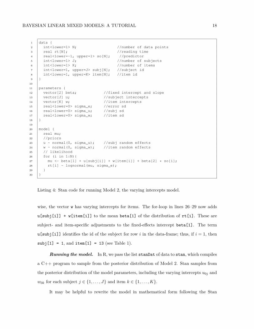
Listing 4: Stan code for running Model 2, the varying intercepts model.

wise, the vector w has varying intercepts for items. The for-loop in lines 26–29 now adds

u[subj[i]] + w[item[i]] to the mean beta[1] of the distribution of rt[i]. These are

subject- and item-specific adjustments to the fixed-effects intercept beta[1]. The term

u[subj[i]] identifies the id of the subject for row i in the data-frame; thus, if i = 1, then

subj[1] = 1, and item[1] = 13 (see Table 1).

Running the model. In R, we pass the list stanDat of data to stan, which compiles

a C++ program to sample from the posterior distribution of Model 2. Stan samples from

the posterior distribution of the model parameters, including the varying intercepts u0j and

w0k for each subject j ∈ {1, . . . , J} and item k ∈ {1, . . . ,K}.

It may be helpful to rewrite the model in mathematical form following the Stan


syntax (Gelman and Hill 2007 use a similar notation); the Stan statements are slightly

different from the way that we expressed Model 2. Defining i as the row id in the data, i.e.,

i ∈ {1, . . . , 547}, we can write:

Likelihood :

µi = β0 + u[subj[i]] + w[item[i]] + β1 · soi

rti ∼ LogNormal(µi, σe)

Priors :

u ∼ Normal(0, σu) w ∼ Normal(0, σw)

σe, σu, σw ∼ Uniform(0,∞)

β ∼ Uniform(−∞,∞)

(3)

Here, notice that the i-th row in the statement for µ identifies the subject id (k)

ranging from 1 to 37, and the item id (k) ranging from 1 to 15.

Summarizing the results. The posterior distributions of each of the parameters

is summarized in Table 3. The R̂ values suggest that model has converged. Note also that

compared to Model 1, the estimate of σe is smaller; this is because the other two variance

components are now being estimated as well. Note that the 95% credible interval for the

estimate β̂1 includes 0; thus, there is some evidence that object relatives are easier than

subject relatives, but we cannot exclude the possibility that there is no difference in the

reading times between the two relative clause types.


β̂0 6.06 5.92 6.20 1β̂1 −0.04 −0.08 0.01 1σ̂e 0.52 0.49 0.55 1σ̂u 0.25 0.19 0.34 1σ̂w 0.20 0.12 0.32 1

Table 3The quantiles and the R̂ statistic in the Gibson and Wu data, the varying intercepts model.


Varying Intercepts, Varying Slopes Mixed Effects Model

Consider now that subjects who are faster than average (i.e., who have a negative

varying intercept) may exhibit greater slowdowns when they read subject relatives compared

to object relatives. Similarly, it is in principle possible that items which are read faster (i.e.,

which have a large negative varying intercept) may show a greater slowdown in subject

relatives than object relatives. The opposite situation could also hold: faster subjects may

show smaller SR-OR effects, or items read faster may show smaller SR-OR effects. Although

such individual-level variability was not of interest in the original paper by Gibson and Wu,

it could be of theoretical interest (see, for example, Kliegl, Wei, Dambacher, Yan, and Zhou

2010). Furthermore, as Barr et al. (2013) point out, it is in principle desirable to include a

fixed effect factor in the random effects as a varying slope if the experiment design is such

that subjects see both levels of the factor (cf. Bates et al. 2015).

In order to express this structure in the LMM, we must make two changes in the

varying intercepts Model 2.

Adding varying slopes. The first change is to let the size of the effect for the

predictor so vary by subject and by item. The goal here is to express that some subjects

exhibit greater slowdowns in the object relative condition than others. We let effect size

vary by subject and by item by including in the model by-subject and by-item varying slopes

which adjust the fixed slope β1 in the same way that the by-subject and by-item varying

intercepts adjust the fixed intercept β0. This adjustment of the slope by subject and by

item is expressed by adjusting β1 by adding two terms u1j and w1k. These are random or

varying slopes, and by adding them we account for how the effect of relative clause type

varies by subject j and by item k. We now express the logarithm of reading time, which

was produced by subject j reading item k, as the following sum. The subscript i indexes

the conditions.

log rtijk = β0 + u0j + w0k︸︷︷︸varying intercepts

+β1 + u1ij + w1ik︸︷︷︸varying slopes

+εijk (4)


Defining a variance-covariance matrix for the random effects. The second

change which we make to Model 2 is to define a covariance relationship between by-subject

varying intercepts and slopes, and between by-items intercepts and slopes. This amounts to

adding an assumption that the by-subject slopes u1 could in principle have some correlation

with the by-subject intercepts u0; and by-item slopes w1 with by-item intercept w0. We

explain this in detail below.

Let us assume that the adjustments u0 and u1 are normally distributed with mean zero

and some variances σ2u0 and σ2

u1, respectively; also assume that u0 and u1 have correlation

ρu. It is standard to express this situation by defining a variance-covariance matrix Σu

(sometime this is simply called a variance matrix). This matrix has the variances of u0

and u1 respectively along the diagonals, and the covariances on the off-diagonals. (The

covariance Cov(X,Y ) between two variables X and Y is defined as the product of their

correlation ρ and their standard deviations σX and σY : Cov(X,Y ) = ρσXσY .)

Σu =

σ2u0 ρuσu0σu1

ρuσu0σu1 σ2u1

(5)

Similarly, we can define a variance-covariance matrix Σw for items, using the standard

deviations σw0, σw1, and the correlation ρw.

Σw =

σ2w0 ρwσw0σw1

ρwσw0σw1 σ2w1

(6)

The standard way to express this relationship between the subject intercepts u0 and

slopes u1, and the item intercepts w0 and slopes w1, is to define a bivariate normal distri-

bution as follows:

u0

u1

∼ N0

0

,Σu

,w0

w1

∼ N0

0

,Σw

(7)

An important point to notice here is that any n × n variance-covariance matrix has


associated with it an n × n correlation matrix. In the subject variance-covariance matrix

Σu, the correlation matrix is

1 ρ01

ρ01 1

(8)

In a correlation matrix, the diagonal elements will always be 1, because a variable

always has a correlation of 1 with itself. The off-diagonals will have the correlations between

the variables. Note also that, given the variances σ2u0 and σ2

u1, we can always recover the

variance-covariance matrix, if we know the correlation matrix. This is because of the above-

mentioned definition of covariance.

A correlation matrix can be decomposed into a square root of the matrix, using the

Cholesky decomposition. Thus, given a correlation matrix C, we can obtain its square root

L; an obvious consequence is that we can square L to get the correlation matrix C back.

This is easy to illustrate with a simple example. Suppose we have a correlation matrix:

C =

1 −0.5

−0.5 1

(9)

We can use the Cholesky decomposition function in R, chol, to derive the lower

triangular square root L of this matrix. This gives us:

L =

1 0

−0.5 0.8660254

(10)

We can confirm that this is a square root by multiplying L with itself to get the corre-

lation matrix back (squaring a matrix is done by multiplying the matrix by its transpose):

LLᵀ =

1 0

−0.5 0.8660254

1 −0.5

0 0.8660254

=

1 −0.5

−0.5 1

(11)

The reason that we bring up the Cholesky decomposition here is that we will use it


−10 −5 0 5 10

−10

−5

05

10

z1

z 2

−10 −5 0 5 10

−10

−5

05

10

x1

x 2

Figure 4 . Uncorrelated random variables z = (z1, z2)ᵀ (left) and correlated random variablesx = (x1, x2)ᵀ (right).

to generate the by-subject and by-item adjustments to the intercept and slope fixed-effects

parameters.

Generating correlated random variables using the Cholesky decomposition.

The by-subject and by-item adjustments are generated using the following standard proce-

dure for generating correlated random variables x = (x1, x2):

1. Given a vector of standard deviances (e.g., σu0, σu1), create a diagonal matrix:

τ =

σu0 0

0 σu0

(12)

2. Premultiply the diagonalized matrix τ with the Cholesky decomposition L of the

correlation matrix C to get a matrix Λ.

3. Generate values from a random variable z = (z1, z2)ᵀ, where z1 and z2 each have

independent N (0, 1) distributions (left panel of Figure 4).

4. Multiply Λ with z; this generates the correlated random variables x (right panel

of Figure 4).

This digression into Cholesky decomposition and the generation of correlated random

variables is important to understand for building the Stan model. We will define a vague

prior distribution on L — the square root of the correlation matrix — and a vague prior on

the standard deviations. This allows us to generate the by-subject and by-item adjustments

to the fixed effects intercepts and slopes.


1 ranIntSlpFit <- stan(file = "ranIntSlp.stan", data = stanDat,2 iter = 2000, chains = 4)3

4 # posterior probability of beta 1 being less5 # than 0:6 beta1 <- unlist(extract(ranIntSlpFit, pars = "beta[2]"))7 print(quantile(beta1, probs = c(0.025, 0.5, 0.975)))8 mean(beta1 < 0)

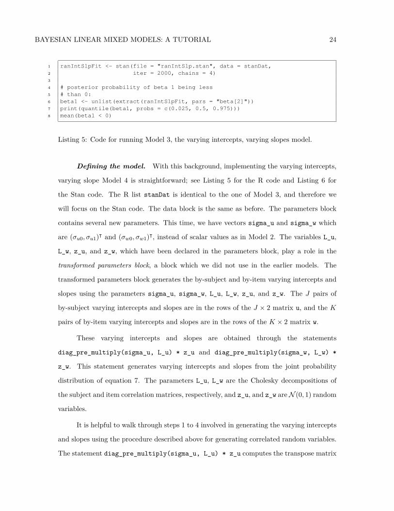
Listing 5: Code for running Model 3, the varying intercepts, varying slopes model.

Defining the model. With this background, implementing the varying intercepts,

varying slope Model 4 is straightforward; see Listing 5 for the R code and Listing 6 for

the Stan code. The R list stanDat is identical to the one of Model 3, and therefore we

will focus on the Stan code. The data block is the same as before. The parameters block

contains several new parameters. This time, we have vectors sigma_u and sigma_w which

are (σu0, σu1)ᵀ and (σw0, σw1)ᵀ, instead of scalar values as in Model 2. The variables L_u,

L_w, z_u, and z_w, which have been declared in the parameters block, play a role in the

transformed parameters block, a block which we did not use in the earlier models. The

transformed parameters block generates the by-subject and by-item varying intercepts and

slopes using the parameters sigma_u, sigma_w, L_u, L_w, z_u, and z_w. The J pairs of

by-subject varying intercepts and slopes are in the rows of the J × 2 matrix u, and the K

pairs of by-item varying intercepts and slopes are in the rows of the K × 2 matrix w.

These varying intercepts and slopes are obtained through the statements

diag_pre_multiply(sigma_u, L_u) * z_u and diag_pre_multiply(sigma_w, L_w) *

z_w. This statement generates varying intercepts and slopes from the joint probability

distribution of equation 7. The parameters L_u, L_w are the Cholesky decompositions of

the subject and item correlation matrices, respectively, and z_u, and z_w areN (0, 1) random

variables.

It is helpful to walk through steps 1 to 4 involved in generating the varying intercepts

and slopes using the procedure described above for generating correlated random variables.

The statement diag_pre_multiply(sigma_u, L_u) * z_u computes the transpose matrix


1 data {2 int<lower=1> N; //number of data points3 real rt[N]; //reading time4 real<lower=-1, upper=1> so[N]; //predictor5 int<lower=1> J; //number of subjects6 int<lower=1> K; //number of items7 int<lower=1, upper=J> subj[N]; //subject id8 int<lower=1, upper=K> item[N]; //item id9 }

10

11 parameters {12 vector[2] beta; //intercept and slope13 real<lower=0> sigma_e; //error sd14 vector<lower=0>[2] sigma_u; //subj sd15 vector<lower=0>[2] sigma_w; //item sd16 cholesky_factor_corr[2] L_u;17 cholesky_factor_corr[2] L_w;18 matrix[2,J] z_u;19 matrix[2,K] z_w;20 }21

22 transformed parameters{23 matrix[2,J] u;24 matrix[2,K] w;25

26 u <- diag_pre_multiply(sigma_u, L_u) * z_u; //subj random effects27 w <- diag_pre_multiply(sigma_w, L_w) * z_w; //item random effects28 }29

30 model {31 real mu;32 //priors33 L_u ~ lkj_corr_cholesky(2.0);34 L_w ~ lkj_corr_cholesky(2.0);35 to_vector(z_u) ~ normal(0,1);36 to_vector(z_w) ~ normal(0,1);37 //likelihood38 for (i in 1:N){39 mu <- beta[1] + u[1,subj[i]] + w[1,item[i]]40 + (beta[2] + u[2,subj[i]] + w[2,item[i]]) * so[i];41 rt[i] ~ lognormal(mu, sigma_e);42 }43 }

Listing 6: The Stan code for Model 3, the varying intercepts, varying slopes model.


product (steps 1 and 2). The right multiplication of this product by z_u, a matrix of

normally distributed random variables (step 3), yields the varying intercepts and slopes

(step 4).

u01 u11

u02 u12...

...

u0J u1J

=(diag(σu0, σu1)Luzu

)ᵀ

=

σu0 0

0 σ01

`11 0

`21 `22

z11 z12 . . . z1J

z21 z22 . . . z2J

ᵀ

(13)

Turning to the model block, here, we place priors on the parameters declared in the

parameters block, and define how these parameters generate log rt (Listing 6, lines 30–42).

The definition of the prior L_u ∼ lkj_corr_cholesky(2.0) implicitly places a so-called

lkj prior with shape parameter η = 2.0 on the correlation matrices

1 ρu

ρu 1

and

1 ρw

ρw 1

, (14)

where ρu is the correlation between the by-subject varying intercept σu0 and slope σu1 (cf.

the covariance matrix of Equation 5) and ρw is the correlation between the by-item varying

intercept σw0 and slope σw1. The lkj distribution with shape parameter η = 1.0 is a uniform

prior over all 2 × 2 correlation matrices; it scales up to larger correlation matrices. The

parameter η has an effect on the shape of the lkj distribution. Our choice of η = 2.0 implies

that the correlations in the off-diagonals are near zero, reflecting the fact that we have no

prior information about the correlation between intercepts and slopes.

The statement to_vector(z_u) ∼ normal(0,1) places a normal distribution with

mean zero and standard deviation one on z_u. The same goes for z_w. The for-loop assigns

to mu the mean of the log-normal distribution from which we draw rt[i], conditional on


the value of the predictor so[i] for relative clause type and the subject and item identity.

We can now fit the varying intercepts, varying slopes Model 3; see Listing 5 for the

code. We see in the model summary in Table 4 that the model has converged, and that

the credible intervals of the parameter of interest, β1, still include 0. In fact, the posterior

probability of the parameter being less than 0 is now 90% (this information can be extracted

as shown in Listing 5, lines 6–8).


β̂0 6.06 5.92 6.21 1β̂1 −0.04 −0.09 0.02 1σ̂e 0.51 0.48 0.55 1σ̂u0 0.25 0.19 0.34 1σ̂u1 0.07 0.01 0.14 1σ̂w0 0.20 0.13 0.32 1σ̂w1 0.04 0.0 0.10 1

Table 4The quantiles and the R̂ statistic in the Gibson and Wu data, the varying intercepts, varyingslopes model.

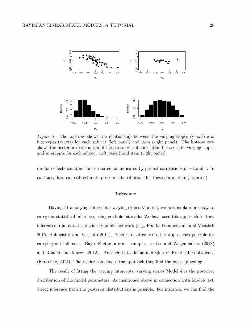
Figure 5 plots the varying slope’s posterior distribution against the varying intercept’s

posterior distribution for each subject. The correlation between u0 and u1 is negative, as

captured by the marginal posterior distributions of the correlation ρu between u0 and u1.

Thus, Figure 5 suggests that the slower a subject’s reading time is on average, the slower

they read object relatives. In contrast, Figure 5 shows no clear pattern for the by-item

varying intercepts and slopes. The broader distribution of the correlation parameter for

items compared to slopes illustrates the greater uncertainty concerning the true value of

the parameter. We briefly discuss inference next.

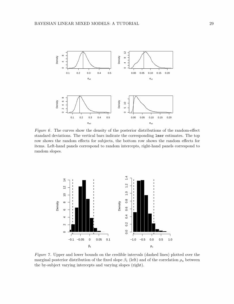
Random effects in a non-Bayesian LMM. We fit the same model also as a

classical non-Bayesian LMM with the lmer function from the lme4 package. This allows for

comparing the results to the Stan results. Here, we focus on random effects. As illustrated

in Figure 6, the estimates of the random-effect standard deviations of the classical LMM are

in agreement with the modes of the posterior distributions. However, the classical LMM is

overparameterized due to an insufficient number of data points. Hence, correlations between


−0.6 −0.4 −0.2 0.0 0.2 0.4 0.6−

0.10

0.00

0.10

u0

u 1

−0.6 −0.4 −0.2 0.0 0.2 0.4 0.6

−0.

100.

000.

10

w0

w1

ρu

Den

sity

−1.0 −0.5 0.0 0.5 1.0

0.0

0.6

1.2

ρwD

ensi

ty

−1.0 −0.5 0.0 0.5 1.0

0.0

0.4

0.8

Figure 5 . The top row shows the relationship between the varying slopes (y-axis) andintercepts (x-axis) for each subject (left panel) and item (right panel). The bottom rowshows the posterior distribution of the parameter of correlation between the varying slopesand intercepts for each subject (left panel) and item (right panel).

random effects could not be estimated, as indicated by perfect correlations of −1 and 1. In

contrast, Stan can still estimate posterior distributions for these parameters (Figure 5).

Inference

Having fit a varying intercepts, varying slopes Model 3, we now explain one way to

carry out statistical inference, using credible intervals. We have used this approach to draw

inferences from data in previously published work (e.g., Frank, Trompenaars, and Vasishth

2015, Hofmeister and Vasishth 2014). There are of course other approaches possible for

carrying out inference. Bayes Factors are an example; see Lee and Wagenmakers (2013)

and Rouder and Morey (2012). Another is to define a Region of Practical Equivalence

(Kruschke, 2014). The reader can choose the approach they find the most appealing.

The result of fitting the varying intercepts, varying slopes Model 4 is the posterior

distribution of the model parameters. As mentioned above in connection with Models 1-3,

direct inference from the posterior distributions is possible. For instance, we can find the


0.1 0.2 0.3 0.4 0.5

04

8

σu0

Den

sity

0.00 0.05 0.10 0.15 0.20

04

812

σu1

Den

sity

0.1 0.2 0.3 0.4 0.5

02

46

8

σw0

Den

sity

0.00 0.05 0.10 0.15 0.20

05

10σw1

Den

sity

Figure 6 . The curves show the density of the posterior distributions of the random-effectstandard deviations. The vertical bars indicate the corresponding lmer estimates. The toprow shows the random effects for subjects, the bottom row shows the random effects foritems. Left-hand panels correspond to random intercepts, right-hand panels correspond torandom slopes.

β1

Den

sity

02

46

810

1214

−0.1 −0.05 0 0.05 0.1

ρu

Den

sity

−1.0 −0.5 0.0 0.5 1.0

0.0

0.2

0.4

0.6

0.8

1.0

1.2

1.4

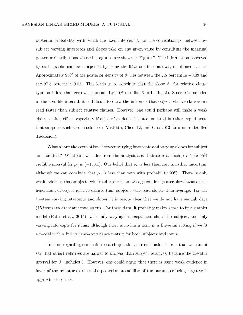
Figure 7 . Upper and lower bounds on the credible intervals (dashed lines) plotted over themarginal posterior distribution of the fixed slope β1 (left) and of the correlation ρu betweenthe by-subject varying intercepts and varying slopes (right).


posterior probability with which the fixed intercept β1 or the correlation ρu between by-

subject varying intercepts and slopes take on any given value by consulting the marginal

posterior distributions whose histograms are shown in Figure 7. The information conveyed

by such graphs can be sharpened by using the 95% credible interval, mentioned earlier.

Approximately 95% of the posterior density of β1 lies between the 2.5 percentile −0.09 and

the 97.5 percentile 0.02. This leads us to conclude that the slope β1 for relative clause

type so is less than zero with probability 90% (see line 8 in Listing 5). Since 0 is included

in the credible interval, it is difficult to draw the inference that object relative clauses are

read faster than subject relative clauses. However, one could perhaps still make a weak

claim to that effect, especially if a lot of evidence has accumulated in other experiments

that supports such a conclusion (see Vasishth, Chen, Li, and Guo 2013 for a more detailed

discussion).

What about the correlations between varying intercepts and varying slopes for subject

and for item? What can we infer from the analysis about these relationships? The 95%

credible interval for ρu is (−1, 0.1). Our belief that ρu is less than zero is rather uncertain,

although we can conclude that ρu is less than zero with probability 90%. There is only

weak evidence that subjects who read faster than average exhibit greater slowdowns at the

head noun of object relative clauses than subjects who read slower than average. For the

by-item varying intercepts and slopes, it is pretty clear that we do not have enough data

(15 items) to draw any conclusions. For these data, it probably makes sense to fit a simpler

model (Bates et al., 2015), with only varying intercepts and slopes for subject, and only

varying intercepts for items; although there is no harm done in a Bayesian setting if we fit

a model with a full variance-covariance matrix for both subjects and items.

In sum, regarding our main research question, our conclusion here is that we cannot

say that object relatives are harder to process than subject relatives, because the credible

interval for β1 includes 0. However, one could argue that there is some weak evidence in

favor of the hypothesis, since the posterior probability of the parameter being negative is

approximately 90%.


Matrix formulation of the linear mixed model

We fit three models with increasing complexity to the data-set. In all specifications,

there was an explicit vector so for the predictor variable in Stan. However, if we want

to fit more complex models with a multitude of categorical and continuous predictors and

interactions, this approach requires increasingly complex specifications in Stan code. Al-

ternatively, we can use the matrix formulation of the linear mixed model that allows for

using the same code for models of different complexity. In the following, we will apply this

approach for an alternative version of Model 3 including random intercepts and slopes for

subjects and items (Equation 4).

Again, we fit a varying intercepts, varying slopes model. The grand mean β0 of log rt

is adjusted by subject and by item through the varying intercepts u0 and w0, which are

unique values for each subject and item respectively. Likewise, the fixed effect β1, which is

associated with the predictor so, is adjusted by the by-subject varying slope u1 and by-item

varying slope w1.

It is more convenient to represent this model in matrix form. We build up the model

specification by first noting that, for each subject, the by-subject varying intercept u0

and slope u1 have a multivariate normal prior distribution with mean zero and covariance

matrix Σu. Similarly, for each item, the by-item varying intercept w0 and slope w1 have a

multivariate normal prior distribution with mean zero and covariance matrix Σw. The error

ε is assumed to have a normal distribution with mean zero and standard deviation σe.

We proceed to implement the model in Stan. Instead of passing the predic-

tor so to stan as vector, as we did earlier, we make so into a design matrix X us-

ing the function model.matrix available in R (see Listing 7, line 2).2 The command

model.matrix(~ 1 + so, rDat) creates a model matrix with two fixed effects, the in-

tercept (1) and a factor (so), based on the data frame rDat. The first column of the design

matrix X consists of all ones; this column represents the intercept. The second column is

2Here, we would like to acknowledge the contribution of Douglas Bates in specifying the model in thisgeneral matrix form.


1 # Make design matrix2 X <- unname(model.matrix(~ 1 + so, rDat))3 attr(X, "assign") <- NULL4 # Make Stan data5 stanDat <- list(N = nrow(X),6 P = ncol(X),7 n_u = ncol(X),8 n_w = ncol(X),9 X = X,

10 Z_u = X,11 Z_w = X,12 J = nlevels(rDat$subj),13 K = nlevels(rDat$item),14 rt = rDat$rt,15 subj = as.integer(rDat$subj),16 item = as.integer(rDat$item))17 # Fit the model18 matrixFit <- stan(file = "matrixModel.stan", data = stanDat,19 iter = 2000, chains = 4)

Listing 7: Matrix formulation code for running the varying intercepts, varying slopes model.

the predictor so and consists of values in {−1, 1}. The model matrix thus consists of a

two-level factorial design, with blocks of this design repeated for each subject. For the full

data-set, we could write it very compactly in matrix form as follows:

log rt = Xβ + Zuu + Zww + ε (15)

Here, X is the N × P model matrix (with N = 547, since we have 547 data points;

and P = 2 since we have the intercept plus another fixed effect), β is a vector of length

P including fixed effects parameters, Zu and Zw are the subject and item model matrices

(N × P ), and u and w are the by-subject and by-item adjustments to the fixed effects

estimates; these are identical to the design matrix X in the model with varying intercepts

and varying slopes included. For more examples of similar model specifications in Stan, see

the R package RePsychLing on github (https://github.com/dmbates/RePsychLing).

Note that we remove the column names and the attributes of the model matrix X in

order to use it for Stan; please refer to Listing 7. Having defined the model, we proceed to


assemble the list stanDat of data, relying on the above matrix formulation. The number

N of observations, the number J of subjects and K of items, the reading times rt, and the

subject and item indicator variables subj and item are familiar from the previous models

presented. The integer P is the number of fixed effects (two including the intercept). Model

4 includes a varying intercept u0 and a varying slope u1 for each subject, and so the number

n_u of by-subject random effects equals P. Likewise, Model 4 includes a varying intercept

w0 and a varying slope w1 for each item, and so the number n_w of by-item random effects

also equals P.

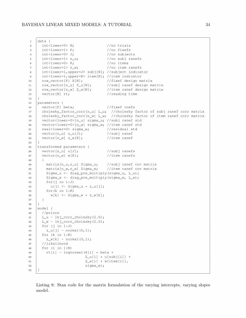
We also have to adapt the Stan code to the model formulation (see Listing 8). The

data block contains the corresponding variables. Using the command row_vector[P] X[N],

we declare the fixed effects design matrix X as an array of N row vectors of length P whose

components are the predictors associated with the N reading times. Likewise for the subject

and item random effects design matrices Z_u and Z_w, which correspond to Zu and Zw

respectively in Equation 15. The vector beta contains the fixed effects β0 and β1. The

matrices L_u, L_w and the arrays z_u, z_w of vectors (not to be confused with the design

matrices Z_u and Z_w) will generate the varying intercepts and slopes u0, u1 and w0, w1,

using the procedure described for Model 3. For example, the command vector[n_u] u[J]

specifies u as an array of J vectors of length n_u; hence, there is one vector per subject.

The vector sigma_u contains the standard deviations of the by-subject varying intercepts

and slopes u0, u1, and the vector sigma_w contains the standard deviations of the by-item

varying intercepts and slopes w0, w1. The variable sigma_e is the standard deviation σe

of the error ε. The transformed parameters block generates the by-subject intercepts and

slopes u0, u1 and the by-item intercepts and slopes w0, w1.

We place lkj priors on the random effects correlation matrices through the

lkj_corr_cholesky(2.0) priors on their Cholesky factors L_u and L_w. We implicitly

place uniform priors on the fixed effects β0, β1, the random effects standard deviations

σu0, σu1, and σw0, σw1 and the error standard deviation σe by omitting any prior specifica-

tions for them in the model block. We specify the likelihood with the probability statement


1 data {2 int<lower=0> N; //no trials3 int<lower=1> P; //no fixefs4 int<lower=0> J; //no subjects5 int<lower=1> n_u; //no subj ranefs6 int<lower=0> K; //no items7 int<lower=1> n_w; //no item ranefs8 int<lower=1,upper=J> subj[N]; //subject indicator9 int<lower=1,upper=K> item[N]; //item indicator

10 row_vector[P] X[N]; //fixef design matrix11 row_vector[n_u] Z_u[N]; //subj ranef design matrix12 row_vector[n_w] Z_w[N]; //item ranef design matrix13 vector[N] rt; //reading time14 }15 parameters {16 vector[P] beta; //fixef coefs17 cholesky_factor_corr[n_u] L_u; //cholesky factor of subj ranef corr matrix18 cholesky_factor_corr[n_w] L_w; //cholesky factor of item ranef corr matrix19 vector<lower=0>[n_u] sigma_u; //subj ranef std20 vector<lower=0>[n_w] sigma_w; //item ranef std21 real<lower=0> sigma_e; //residual std22 vector[n_u] z_u[J]; //subj ranef23 vector[n_w] z_w[K]; //item ranef24 }25 transformed parameters {26 vector[n_u] u[J]; //subj ranefs27 vector[n_w] w[K]; //item ranefs28 {29 matrix[n_u,n_u] Sigma_u; //subj ranef cov matrix30 matrix[n_w,n_w] Sigma_w; //item ranef cov matrix31 Sigma_u <- diag_pre_multiply(sigma_u, L_u);32 Sigma_w <- diag_pre_multiply(sigma_w, L_w);33 for(j in 1:J)34 u[j] <- Sigma_u * z_u[j];35 for(k in 1:K)36 w[k] <- Sigma_w * z_w[k];37 }38 }39 model {40 //priors41 L_u ~ lkj_corr_cholesky(2.0);42 L_w ~ lkj_corr_cholesky(2.0);43 for (j in 1:J)44 z_u[j] ~ normal(0,1);45 for (k in 1:K)46 z_w[k] ~ normal(0,1);47 //likelihood48 for (i in 1:N)49 rt[i] ~ lognormal(X[i] * beta +50 Z_u[i] * u[subj[i]] +51 Z_w[i] * w[item[i]],52 sigma_e);53 }

Listing 8: Stan code for the matrix formulation of the varying intercepts, varying slopesmodel.


that rt[i] is distributed log-normally with mean X[i] * beta + Z_u[i] * u[subj[i]]

+ Z_w[i] * w[item[i]] and standard deviation sigma_e. The next step towards model-

fitting is to pass the list stanDat to stan, which compiles a C++ program to sample from

the posterior distribution of the model parameters.

A major advantage of the above matrix formulation is that we do not need to write a

new Stan model for a future repeated measures design. All we have to do now is define the

design matrix X appropriately, and include it (along with appropriately defined Zu and Zw

for the subjects and items random effects) as part of the data specification that is passed

to Stan.

Concluding remarks, and further reading

We hope that this tutorial has given the reader a flavor of what it would be like to

fit Bayesian linear mixed models. There is of course much more to say on the topic, and

we hope that the interested reader will take a look at some of the excellent books that

have recently come out. We suggest below a sequence of reading that we found helpful.

A good first general textbook is by Gelman and Hill (2007); it begins with the frequen-

tist approach and only later transitions to Bayesian models. The forthcoming book by

Mcelreath (2016) is also excellent. For those looking for a psychology-specific introduc-

tion, the books by Kruschke (2014) and Lee and Wagenmakers (2013) are to be recom-

mended, although for the latter the going might be easier if the reader has already looked

at Gelman and Hill (2007). As a second book, Lunn et al. (2012) is recommended; it

provides many interesting and useful examples using the BUGS language, which are dis-

cussed in exceptionally clear language. Many of these books use the BUGS syntax (Lunn

et al., 2000), which the probabilistic programming language JAGS (Plummer, 2012) also

adopts; however, Stan code for these books is slowly becoming available on the Stan home

page (https://github.com/stan-dev/example-models/wiki). For those with introduc-

tory calculus, a slightly more technical introduction to Bayesian methods by Lynch (2007)

is an excellent choice. Finally, the textbook by Gelman et al. (2014) is the definitive modern


guide, and provides a more advanced treatment.

Acknowledgements

We are grateful to the developers of Stan (in particular, Andrew Gelman, Bob Car-

penter) and members of the Stan mailing list for their advice regarding model specification.

Douglas Bates and Reinhold Kliegl have helped considerably over the years in improving

our understanding of LMMs from a frequentist perspective. We also thank Edward Gibson

for releasing his published data. Titus von der Malsburg and Bruno Nicenboim provided

useful comments on a draft.


References

Barr, D. J., Levy, R., Scheepers, C., & Tily, H. J. (2013). Random effects structure for

confirmatory hypothesis testing: Keep it maximal. Journal of Memory and Language,

68 (3), 255–278.

Bates, D., Kliegl, R., Vasishth, S., & Baayen, H. (2015). Parsimonious mixed models.

Retrieved from http://arxiv.org/abs/1506.04967 (ArXiv e-print; submitted to

Journal of Memory and Language)

Bates, D., Maechler, M., Bolker, B. M., & Walker, S. (2014). lme4: Linear mixed-

effects models using eigen and s4. Retrieved from http://arxiv.org/abs/1406.5823

(ArXiv e-print; submitted to Journal of Statistical Software)

Frank, S. L., Trompenaars, T., & Vasishth, S. (2015). Cross-linguistic differences in pro-

cessing double-embedded relative clauses: Working-memory constraints or language

statistics? Cognitive Science, n/a.

Gelman, A., Carlin, J. B., Stern, H. S., Dunson, D. B., Vehtari, A., & Rubin, D. B. (2014).

Bayesian data analysis (Third ed.). Chapman and Hall/CRC.

Gelman, A., & Hill, J. (2007). Data analysis using regression and multilevel/hierarchical

models. Cambridge, UK: Cambridge University Press.

Gelman, A., & Rubin, D. B. (1992). Inference from iterative simulation using multiple

sequences. Statistical science, 457–472.

Gibson, E., & Wu, H.-H. I. (2013). Processing Chinese relative clauses in context. Language

and Cognitive Processes, 28 (1-2), 125–155.

Hofmeister, P., & Vasishth, S. (2014). Distinctiveness and encoding effects in online sentence

comprehension. , 5 , 1–13. (Article 1237) doi: doi:10.3389/fpsyg.2014.01237

Hsiao, F. P.-F., & Gibson, E. (2003). Processing relative clauses in Chinese. Cognition,

90 , 3–27.

Just, M., & Carpenter, P. (1992). A capacity theory of comprehension: Individual differ-

ences in working memory. Psychological Review, 99 (1), 122–149.

Kliegl, R., Wei, P., Dambacher, M., Yan, M., & Zhou, X. (2010). Experimental effects and


individual differences in linear mixed models: Estimating the relationship between

spatial, object, and attraction effects in visual attention. Frontiers in Psychology, 1 .

Kruschke, J. (2014). Doing Bayesian Data Analysis: A tutorial introduction with R, JAGS,

and Stan. Academic Press.

Lavine, M. (1999). What is Bayesian statistics and why everything else is wrong. The

Journal of Undergraduate Mathematics and its applications, 20 , 165–174.

Lee, M. D., & Wagenmakers, E.-J. (2013). Bayesian cognitive modeling: A practical course.

Cambridge University Press.

Lunn, D., Jackson, C., Spiegelhalter, D. J., Best, N., & Thomas, A. (2012). The BUGS

book: A practical introduction to Bayesian analysis (Vol. 98). CRC Press.

Lunn, D., Thomas, A., Best, N., & Spiegelhalter, D. (2000). WinBUGS — A Bayesian

modelling framework: Concepts, structure, and extensibility. Statistics and comput-

ing, 10 (4), 325–337.

Lynch, S. M. (2007). Introduction to applied Bayesian statistics and estimation for social

scientists. Springer.

Mcelreath, R. (2016). Statistical rethinking: A Bayesian course with R examples. Chapman

and Hall. (To appear)

Morey, R. D., Hoekstra, R., Rouder, J. N., Lee, M. D., & Wagenmakers, E.-J. (2015). The

fallacy of placing confidence in confidence intervals.

Pinheiro, J. C., & Bates, D. M. (2000). Mixed-effects models in S and S-PLUS. New York:

Springer-Verlag.

Plummer, M. (2012). JAGS version 3.3.0 manual. International Agency for Research on

Cancer. Lyon, France.

R Development Core Team. (2006). R: A language and environment for statistical com-

puting [Computer software manual]. Vienna, Austria. Retrieved from http://

www.R-project.org (ISBN 3-900051-07-0)

Raftery, A. E., & Lewis, S. (1992). How many iterations in the Gibbs sampler? In

J. Bernardo, J. Berger, A. Dawid, & A. Smith (Eds.), Bayesian statistics 4 (pp.


763–773). Oxford University Press.

Rouder, J. N. (2005). Are unshifted distributional models appropriate for response time?

Psychometrika, 70 , 377–381.

Rouder, J. N., & Morey, R. D. (2012). Default Bayes factors for model selection in regression.

Multivariate Behavioral Research, 47 (6), 877–903.

Spiegelhalter, D. J., Abrams, K. R., & Myles, J. P. (2004). Bayesian approaches to clinical

trials and health-care evaluation (Vol. 13). John Wiley & Sons.

Stan Development Team. (2014). Stan modeling language users guide and reference manual,

version 2.4 [Computer software manual]. Retrieved from http://mc-stan.org/

Vasishth, S., Chen, Z., Li, Q., & Guo, G. (2013, 10). Processing Chinese relative clauses:

Evidence for the subject-relative advantage. PLoS ONE , 8 (10), e77006. doi: 10.1371/

journal.pone.0077006

Xie, Y. (2013). knitr: A general-purpose package for dynamic report generation in R. R

package version, 1 (7).

bayesian linear mixed models using stan: a tutorial for...

Documents