bayesian machine learning via category theory machine learning via category theory jared culbertson...
TRANSCRIPT

Bayesian Machine Learning via Category Theory
Jared Culbertson and Kirk Sturtz
December 6, 2013
Abstract
From the Bayesian perspective, the category of conditional probabilities (a vari-ant of the Kleisli category of the Giry monad, whose objects are measurable spacesand arrows are Markov kernels) gives a nice framework for conceptualization andanalysis of many aspects of machine learning. Using categorical methods, we con-struct models for parametric and nonparametric Bayesian reasoning on functionspaces, thus providing a basis for the supervised learning problem. In particular,stochastic processes are arrows to these function spaces which serve as prior prob-abilities. The resulting inference maps can often be analytically constructed in thissymmetric monoidal weakly closed category. We also show how to view generalstochastic processes using functor categories and demonstrate the Kalman filter asan archetype for the hidden Markov model.
Keywords: Bayesian machine learning, categorical probability, Bayesian probability
Contents
1 Introduction 2
2 The Category of Conditional Probabilities 62.1 (Weak) Product Spaces and Joint Distributions . . . . . . . . . . . . . . . . 82.2 Constructing a Joint Distribution Given Conditionals . . . . . . . . . . . . . 122.3 Constructing Regular Conditionals given a Joint Distribution . . . . . . . . 13
3 The Bayesian Paradigm using P 15
4 Elementary applications of Bayesian probability 18
5 The Tensor Product 255.1 Graphs of Conditional Probabilities . . . . . . . . . . . . . . . . . . . . . . . . 275.2 A Tensor Product of Conditionals . . . . . . . . . . . . . . . . . . . . . . . . . 295.3 Symmetric Monoidal Categories . . . . . . . . . . . . . . . . . . . . . . . . . . 29
arX
iv:1
312.
1445
v1 [
mat
h.C
T]
5 D
ec 2
013

1 INTRODUCTION 2
6 Function Spaces 316.1 Stochastic Processes . . . . . . . . . . . . . . . . . . . . . . . . . . . . . . . . . 366.2 Gaussian Processes . . . . . . . . . . . . . . . . . . . . . . . . . . . . . . . . . . 406.3 GPs via Joint Normal Distributions . . . . . . . . . . . . . . . . . . . . . . . . 41
7 Bayesian Models for Function Estimation 437.1 Nonparametric Models . . . . . . . . . . . . . . . . . . . . . . . . . . . . . . . 43
7.1.1 Noise Free Measurement Model . . . . . . . . . . . . . . . . . . . . . . 447.1.2 Gaussian Additive Measurement Noise Model . . . . . . . . . . . . . 46
7.2 Parametric Models . . . . . . . . . . . . . . . . . . . . . . . . . . . . . . . . . . 50
8 Constructing Inference Maps 548.1 The noise free inference map . . . . . . . . . . . . . . . . . . . . . . . . . . . . 548.2 The noisy measurement inference map . . . . . . . . . . . . . . . . . . . . . . 598.3 The inference map for parametric models . . . . . . . . . . . . . . . . . . . . 61
9 Stochastic Processes as Points 659.1 Markov processes via Functor Categories . . . . . . . . . . . . . . . . . . . . 659.2 Hidden Markov Models . . . . . . . . . . . . . . . . . . . . . . . . . . . . . . . 68
10 Final Remarks 69
11 Appendix A: Integrals over probability measures. 71
12 Appendix B: The weak closed structure in P 72
13 References 72
1 Introduction
Speculation on the utility of using categorical methods in machine learning (ML) hasbeen expounded by numerous people, including by the denizens at the n-category cafeblog [5] as early as 2007. Our approach to realizing categorical ML is based upon viewingML from a probabilistic perspective and using categorical Bayesian probability. Severalrecent texts (e.g., [2, 19]), along with countless research papers on ML have emphasizedthe subject from the perspective of Bayesian reasoning. Combining this viewpoint withthe recent work [6], which provides a categorical framework for Bayesian probability, wedevelop a category theoretic perspective on ML. The abstraction provided by categorytheory serves as a basis not only for an organization of ones thoughts on the subject, butalso provides an efficient graphical method for model building in much the same way thatprobabilistic graphical modeling (PGM) has provided for Bayesian network problems.
In this paper, we focus entirely on the supervised learning problem, i.e., the regressionor function estimation problem. The general framework applies to any Bayesian machine

1 INTRODUCTION 3
learning problem, however. For instance, the unsupervised clustering or density estimationproblems can be characterized in a similar way by changing the hypothesis space andsampling distribution. For simplicity, we choose to focus on regression and leave theother problems to the industrious reader. For us, then, the Bayesian learning problemis to determine a function f ∶ X → Y which takes an input x ∈ X, such as a featurevector, and associates an output (or class) f(x) with x. Given a measurement (x, y),or a set of measurements (xi, yi)Ni=1 where each yi is a labeled output (i.e., trainingdata), we interpret this problem as an estimation problem of an unknown function fwhich lies in Y X , the space of all measurable functions1 from X to Y such that f(xi) ≈ yi.When Y is a vector space the space Y X is also a vector space that is infinite dimensionalwhen X is infinite. If we choose to allow all such functions (every function f ∈ Y X isa valid model) then the problem is nonparametric. On the other hand, if we only allowfunctions from some subspace V ⊂ Y X of finite dimension p, then we have a parametricmodel characterized by a measurable map i ∶ Rp → Y X . The image of i is then thespace of functions which we consider as valid models of the unknown function for theBayesian estimation problem. Hence, the elements a ∈ Rp
completely determine the validmodeling functions i(a) ∈ Y X . Bayesian modeling splits the problem into two aspects:(1) specification of the hypothesis space, which consist of the “valid” functions f , and (2)a noisy measurement model such as yi = f(xi)+ εi, where the noise component εi is oftenmodeled by a Gaussian distribution. Bayesian reasoning with the hypothesis space takenas Y X or any subspace V ⊂ Y X (finite or infinite dimensional) and the noisy measurementmodel determining a sampling distribution can then be used to efficiently estimate (learn)the function f without over fitting the data.
We cast this whole process into a graphical formulation using category theory, whichlike PGM, can in turn be used as a modeling tool itself. In fact, we view the components ofthese various models, which are just Markov kernels, as interchangeable parts. An impor-tant piece of the any solving the ML problem with a Bayesian model consists of choosingthe appropriate parts for a given setting. The close relationship between parametric andnonparametric models comes to the forefront in the analysis with the measurable mapi ∶ Rp → Y X connecting the two different types of models. To illustrate this point supposewe are given a normal distribution P on Rp
as a prior probability on the unknown param-eters. Then the push forward measure2 of P by i is a Gaussian process, which is a basictool in nonparametric modeling. When composed with a noisy measurement model, thisprovides the whole Bayesian model required for a complete analysis and an inference map
1Recall that a σ-algebra ΣX on X is a collection of subsets of X that is closed under complementsand countable unions (and hence intersections); the pair (X,ΣX) is called a measurable space and anyset A ∈ ΣX is called a measurable set of X. A measurable function f ∶X → Y is defined by the propertythat for any measurable set B in the σ-algebra of Y , we have that f−1(B) is in the σ-algebra of X. Forexample, all continuous functions are measurable with respect to the Borel σ-algebras.
2A measure µ on a measurable space (X,ΣX) is a nonnegative real-valued function µ∶X → R≥0 suchthat µ(∅) = 0 and µ(∪∞i=1Ai) = ∑∞i=1 µ(Ai). A probability measure is a measure where µ(X) = 1. In thispaper, all measures are probability measures and the terminology “distribution” will be synonymous with“probability measure.”

1 INTRODUCTION 4
can be analytically constructed.3 Consequently, given any measurement (x, y) taking theinference map conditioned at (x, y) yields the updated prior probability which is anothernormal distribution on Rp
.The ability to do Bayesian probability involving function spaces relies on the fact that
the category of measurable spaces, Meas, has the structure of a symmetric monoidalclosed category (SMCC). Through the evaluation map, this in turn provides the categoryof conditional probabilities P with the structure of a symmetric monoidal weakly closedcategory (SMwCC), which is necessary for modeling stochastic processes as probabilitymeasures on function spaces. On the other hand, the ordinary product X × Y withits product σ-algebra is used for the Bayesian aspect of updating joint (and marginal)distributions. From a modeling viewpoint, the SMwCC structure is used for carryingalong a parameter space (along with its relationship to the output space through theevaluation map). Thus we can describe training data and measurements as ordered pairs(xi, yi) ∈X ⊗ Y , where X plays the role of a parameter space.
A few notes on the exposition. In this paper our intended audience consists of (1)the practicing ML engineer with only a passing knowledge of category theory (e.g., know-ing about objects, arrows and commutative diagrams), and (2) those knowledgeable ofcategory theory with an interest of how ML can be formulated within this context. Forthe ML engineer familiar with Markov kernels, we believe that the presentation of P andits applications can serve as an easier introduction to categorical ideas and methods thanmany standard approaches. While some terminology will be unfamiliar, the examplesshould provide an adequate understanding to relate the knowledge of ML to the cate-gorical perspective. If ML researchers find this categorical perspective useful for furtherdevelopments or simply for modeling purposes, then this paper will have achieved its goal.
In the categorical framework for Bayesian probability, Bayes’ equation is replacedby an integral equation where the integrals are defined over probability measures. Theanalysis requires these integrals be evaluated on arbitrary measurable sets and this isoften possible using the three basic rules provided in Appendix A. Detailed knowledge ofmeasure theory is not necessary outside of understanding these three rules and the basicsof σ-algebras and measures, which are used extensively for evaluating integrals in thispaper. Some proofs require more advanced measure-theoretic ideas, but the proofs cansafely be avoided by the unfamiliar reader and are provided for the convenience of thosewho might be interested in such details.
For the category theorist, we hope the paper makes the fundamental ideas of MLtransparent, and conveys our belief that Bayesian probability can be characterized cate-gorically and usefully applied to fields such as ML. We believe the further developmentof categorical probability can be motivated by such applications and in the final remarkswe comment on one such direction that we are pursuing.
These notes are intended to be tutorial in nature, and so contain much more detailthat would be reasonable for a standard research paper. As in this introductory section,
3The inference map need not be unique.

1 INTRODUCTION 5
basic definitions will be given as footnotes, while more important definitions, lemmas andtheorems Although an effort has been made to make the exposition as self-contained aspossible, complete self-containment is clearly an unachievable goal. In the presentation,we avoid the use of the terminology of random variables for two reasons: (1) formallya random variable is a measurable function f ∶ X → Y and a probability measure P onX gives rise to the distribution of the random variable f⋆(P ) which is the push forwardmeasure of P . In practice the random variable f itself is more often than not impossibleto characterize functionally (consider the process of flipping a coin), while reference tothe random variable using a binomial distribution, or any other distribution, is simplymaking reference to some probability measure. As a result, in practice the term “randomvariable” is often not making reference to any measurable function f and the pushforwardmeasure of some probability measure P at all but rather is just referring to a probabilitymeasure; (2) the term “random variable” has a connotation that, we believe, should bede-emphasized in a Bayesian approach to modeling uncertainty. Thus while a randomvariable can be modeled as a push forward probability measure within the frameworkpresented we feel no need to single them out as having any special relevance beyond theremark already given. In illustrating the application of categorical Bayesian probabilitywe do however show how to translate the familiar language of random variables into theunfamiliar categorical framework for the particular case of Gaussian distributions whichare the most important application for ML since Gaussian Processes are characterized onfinite subsets by Gaussian distributions. This provides a particularly nice illustration ofthe non uniqueness of conditional sampling distribution and inference pairs given a jointdistribution.
Organization. The paper is organized as follows: The theory of Bayesian probability inP is first addressed and applied to elementary problems on finite spaces where the detailedsolutions to inference, prediction and decision problems are provided. If one understandsthe “how and why” in solving these problems then the extension to solving problemsin ML is a simple step as one uses the same basic paradigm with only the hypothesisspace changed to a function space. Nonparametric modeling is presented next, and thenthe parametric model can seen as a submodel of the nonparametric model. We thenproceed to give a general definition of stochastic process as a special type of arrow ina functor category PX , and by varying the category X or placing conditions on theprojection maps onto subspaces one obtains the various types of stochastic processes suchas Markov processes or GP. Finally, we remark on the area where category theory mayhave the biggest impact on applications for ML by integrating the probabilistic modelswith decision theory into one common framework.
The results presented here derived from a categorical analysis of the ML problem(s)will come as no surprise to ML professionals. We acknowledge and thank our colleagueswho are experts in the field who provided assistance and feedback.

2 THE CATEGORY OF CONDITIONAL PROBABILITIES 6
2 The Category of Conditional Probabilities
The development of a categorical basis for probability was initiated by Lawvere [16],and further developed by Giry [14] using monads to characterize the adjunction givenin Lawvere’s original work. The Kleisli category of the Giry monad G is what Lawverecalled the category of probabilistic mappings and what we shall refer to as the categoryof conditional probabilities.4 Further progess was given in the unpublished dissertation ofMeng [18] which provides a wealth of information and provides a basis for thinking aboutstochastic processes from a categorical viewpoint. While this work does not address theBayesian perspective it does provide an alternative “statistical viewpoint” toward solvingsuch problems using generalized metrics. Additional interesting work on this category ispresented in a seminar by Voevodsky, in Russian, available in an online video [22]. Theextension of categorical probability to the Bayesian viewpoint is given in the paper [6],though Lawvere and Peter Huber were aware of a similar approach in the 1960’s.5 Coeckeand Speckens [4] provide an alternative graphical language for Bayesian reasoning underthe assumption of finite spaces which they refer to as standard probability theory. In suchspaces the arrows can be represented by stochastic matrices [13]. More recently Fong [12]has provided further applications of the category of conditional probabilities to CausalTheories for Bayesian networks.
Much of the material in this section is directly from [6], with some additional expla-nation where necessary. The category6 of conditional probabilities, which we denote byP, has countably generated7 measurable spaces (X,ΣX) as objects and an arrow betweentwo such objects
(X,ΣX) (Y,ΣY )T
is a Markov kernel (also called a regular conditional probability) assigning to each elementx ∈ X and each measurable set B ∈ ΣY the probability of B given x, denoted T (B ∣x). The term “regular” refers to the fact that the function T is conditioned on pointsrather than measurable sets A ∈ ΣX . When (X,ΣX) is a countable set (either finite orcountably infinite) with the discrete σ-algebra then every singleton x is measurable andthe term “regular” is unnecessary. More precisely, an arrow T ∶X → Y in P is a functionT ∶ ΣY ×X → [0,1] satisfying
4Monads had not yet been developed at the time of Lawvere’s work. However the adjunction con-struction he provided was the Giry monad on measurable spaces.
5In a personal communication Lawvere related that he and Peter Huber gave a seminar in Zuricharound 1965 on “Bayesian sections.” This refers to the existence of inference maps in the Eilenberg–Moore category of G-algebras. These inference maps are discussed in Section 3, although we discuss themonly in the context of the category P.
6A category is a collection of (1) objects and (2) morphisms (or arrows) between the objects (includinga required identity morphism for each object), along with a prescribed method for associative compositionof morphisms.
7A space (X,ΣX) is countably generated if there exist a countable set of measurable sets Ai∞i=1which generated the σ-algebra ΣX .

2 THE CATEGORY OF CONDITIONAL PROBABILITIES 7
1. for all B ∈ ΣY , the function T (B ∣ ⋅)∶X → [0,1] is measurable, and
2. for all x ∈ X, the function T (⋅ ∣ x)∶ΣY → [0,1] is a perfect probability measure8 onY .
For technical reasons it is necessary that the probability measures in (2) constitute anequiperfect family of probability measures to avoid pathological cases which prevent theexistence of inference maps necessary for Bayesian reasoning.9
The notation T (B ∣ x) is chosen as it coincides with the standard notation “p(H ∣D)”of conditional probability theory. For an arrow T ∶ (X,ΣX) → (Y,ΣY ), we occasionallydenote the measurable function T (B ∣ ⋅)∶ΣY → [0,1] by TB and the probability measureT (⋅ ∣ x)∶ΣY → [0,1] by Tx. Hereafter, for notational brevity we write a measurable space(X,ΣX) simply as X when referring to a generic σ-algebra ΣX .
Given two arrows
X Y ZT U
the composition U T ∶ΣZ ×X → [0,1] is marginalization over Y defined by
(U T )(C ∣ x) = ∫y∈Y
U(C ∣ y)dTx.
The integral of any real valued measurable function f ∶X → R with respect to anymeasure P on X is
EP [f] = ∫x∈X
f(x)dP, (1)
called the P -expectation of f . Consequently the composite (U T )(C ∣ x) is the Tx-expectation of UC ,
(U T )(C ∣ x) = ETx[UC].LetMeas denote the category of measurable spaces where the objects are measurable
spaces (X,ΣX) and the arrows are measurable functions f ∶X → Y . Every measurablemapping f ∶X → Y may be regarded as a P arrow
X Yδf
defined by the Dirac (or one point) measure
δf ∶ X ×ΣY → [0,1]
∶ (B ∣ x) ↦ 1 If f(x) ∈ B0 If f(x) ∉ B.
8A perfect probability measure P on Y is a probability measure such that for any measurable functionf ∶ Y → R there exist a real Borel set E ⊂ f(Y ) satisfying P (f−1(E)) = 1.
9Specifically, the subsequent Theorem 1 is a constructive procedure which requires perfect probabilitymeasures. Corollary 2 then gives the inference map. Without the hypothesis of perfect measures apathological counterexample can be constructed as in [9, Problem 10.26]. The paper by Faden [11] givesconditions on the existence of conditional probabilities and this constraint is explained in full detail in[6]. Note that the class of perfect measures is quite broad and includes all probability measures definedon Polish spaces.
2 THE CATEGORY OF CONDITIONAL PROBABILITIES 8
The relation between the dirac measure and the characteristic (indicator) function 1 is
δf(B ∣ x) = 1f−1(B)(x)
and this property is used ubiquitously in the analysis of integrals.Taking the measurable mapping f to be the identity map on X gives for each object
X the morphism XδIdXÐ→ X given by
δIdX(B ∣ x) = 1 if x ∈ B0 if x ∉ B
which is the identity morphism for X in P. Using standard notation we denote the identitymapping on any object X by 1X = δIdX , or for brevity simply by 1 if the space X is clearfrom the context. With these objects and arrows, law of composition, associativity, andidentity, standard measure-theoretic arguments show that P forms a category.
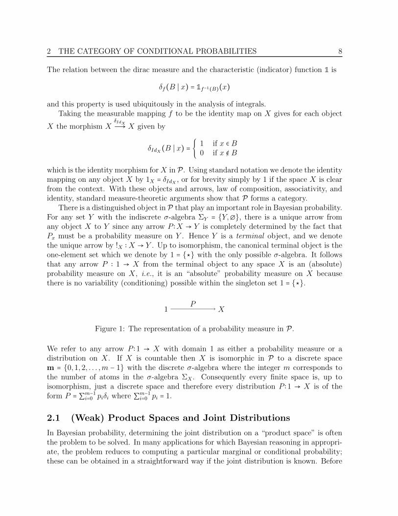
There is a distinguished object in P that play an important role in Bayesian probability.For any set Y with the indiscrete σ-algebra ΣY = Y,∅, there is a unique arrow fromany object X to Y since any arrow P ∶X → Y is completely determined by the fact thatPx must be a probability measure on Y . Hence Y is a terminal object, and we denotethe unique arrow by !X ∶X → Y . Up to isomorphism, the canonical terminal object is theone-element set which we denote by 1 = ⋆ with the only possible σ-algebra. It followsthat any arrow P ∶ 1 → X from the terminal object to any space X is an (absolute)probability measure on X, i.e., it is an “absolute” probability measure on X becausethere is no variability (conditioning) possible within the singleton set 1 = ⋆.
1 XP
Figure 1: The representation of a probability measure in P.
We refer to any arrow P ∶1 → X with domain 1 as either a probability measure or adistribution on X. If X is countable then X is isomorphic in P to a discrete spacem = 0,1,2, . . . ,m − 1 with the discrete σ-algebra where the integer m corresponds tothe number of atoms in the σ-algebra ΣX . Consequently every finite space is, up toisomorphism, just a discrete space and therefore every distribution P ∶1 → X is of theform P = ∑m−1
i=0 piδi where ∑m−1i=0 pi = 1.
2.1 (Weak) Product Spaces and Joint Distributions
In Bayesian probability, determining the joint distribution on a “product space” is oftenthe problem to be solved. In many applications for which Bayesian reasoning in appropri-ate, the problem reduces to computing a particular marginal or conditional probability;these can be obtained in a straightforward way if the joint distribution is known. Before

2 THE CATEGORY OF CONDITIONAL PROBABILITIES 9
proceeding to formulate precisely what the term “product space” means in P, we describethe categorical construct of a finite product space in any category.
Let C be an arbitary category and X,Y ∈ob C. We say the product of X and Y existsif there is an object, which we denote by X × Y , along with two arrows pX ∶X × Y → Xand pY ∶X × Y → Y in C such that given any other object T in C and arrows f ∶ T → Xand g ∶ T → Y there is a unique C arrow ⟨f, g⟩∶T →X × Y that makes the diagram
T
X YX × Y
f g⟨f, g⟩
pX pY
(2)
commute. If the given diagram is a product then we often write the product as a triple(X × Y, pX , pY ). We must not let the notation deceive us; the object X × Y could justas well be represented by PX,Y . The important point is that it is an object in C that weneed to specify in order to show that binary products exist. Products are an example of auniversal construction in categories. The term “universal” implies that these constructionsare unique up to a unique isomorphism. Thus if (PX,Y , pX , py) and (QX,Y , qX , qY ) areboth products for the objects X and Y then there exist unique arrows α∶PX,Y → QX,Y
and β∶QX,Y → PX,Y in C such that β α = 1PX,Y and αβ = 1QX,Y so that the objects PX,Yand QX,Y are isomorphic.
If the product of all object pairs X and Y exist in C then we say binary productsexist in C. The existence of binary products implies the existence of arbitrary finiteproducts in C. So if XiNi=1 is a finite set of objects in C then there is an object which wedenote by ∏N
i=1Xi (in general, this need not be the cartesian product) as well as arrowspXj ∶∏N
i=1Xi →XjNj=1. Then if we are given an arbitrary T ∈ob C and a family of arrowsfj ∶ T → Xj in C there exists a unique C arrow ⟨f1, . . . , fN⟩ such that for every integerj ∈ 1,2, . . . ,N the diagram
T
Xj
N
∏i=1
Xi
fj⟨f1, . . . , fN⟩
pXj
commutes. The arrows pXi defining a product space are often called the projection mapsdue to the analogy with the cartesian products in the category of sets, Set.
2 THE CATEGORY OF CONDITIONAL PROBABILITIES 10
In Set, the product of two sets X and Y is the cartesian product X × Y consisting ofall pairs (x, y) of elements with x ∈X and y ∈ Y along with the two projection mappingsπX ∶X × Y → X sending (x, y) ↦ x and πY ∶X × Y → Y sending (x, y) ↦ y. Given anypair of functions f ∶T → X × Y and g∶T → X × Y the function ⟨f, g⟩∶T → X × Y sendingt↦ (f(t), g(t)) clearly makes Diagram 2 commute. But it is also the unique such functionbecause if γ∶T → X × Y were any other function making the diagram commute then theequations
(pX γ)(t) = f(t) and (pY γ)(t) = g(t) (3)
would also be satisfied. But since the function γ has codomain X × Y which consistof ordered pairs (x, y) it follows that for each t ∈ T that γ(t) = ⟨γ1(t), γ2(t)⟩ for somefunctions γ1∶T → X and γ2∶T → Y . Substituting γ = ⟨γ1, γ2⟩ into equations 3 it followsthat
f(t) = (pX (⟨γ1, γ2⟩))(t) = pX(γ1(t), γ2(t)) = γ1(t)g(t) = (pY (⟨γ1, γ2⟩))(t) = pY (γ2(t), γ2(t)) = γ2(t)
from which it follows γ = ⟨γ1, γ2⟩ = ⟨f, g⟩ thereby proving that there exist at most onesuch function T →X ×Y making the requisite Diagram 2 commute. If the requirement ofthe uniqueness of the arrow ⟨f, g⟩ in the definition of a product is dropped then we havethe definition of a weak product of X and Y .
Given the relationship between the categories P andMeas it is worthwhile to examineproducts in Meas. Given X,Y ∈ob Meas the product X × Y is the cartesian productX ×Y of sets endowed with the smallest σ-algebra such that the two set projection mapsπX ∶X × Y →X sending (x, y)↦ x and πY ∶X × Y → Y sending (x, y)↦ y are measurable.In other words, we take the smallest subset of the powerset of X × Y such that for allA ∈ ΣX and for all B ∈ ΣY the preimages π−1
X (A) = A × Y and π−1Y (B) = X × B are
measurable. Since a σ-algebra requires that the intersection of any two measurable setsis also measurable it follows that π−1
X (A) ∩ π−1Y (B) = A × B must also be measurable.
Measurable sets of the form A × B are called rectangles and generate the collection ofall measurable sets defining the σ-algebra ΣX×Y in the sense that ΣX×Y is equal to theintersection of all σ-algebras containing the rectangles. When the σ-algebra on a set isdetermined by the a family of maps pk∶X×Y → Zkk∈K , whereK is some indexing set suchthat all of these maps pk are measurable we say the σ-algebra is induced (or generated) bythe family of maps pkk∈K .10 The cartesian product X × Y with the σ-algebra inducedby the two projection maps πX and πY is easily verified to be a product of X and Ysince given any two measurable maps f ∶Z → X and g∶Z → Y the map ⟨f, g⟩∶Z → X × Ysending z ↦ (f(z), g(z)) is the unique measurable map satisfying the defining propertyof a product for (X × Y,πX , πY ). This σ-algebra induced by the projection maps πX andπY is called the product σ-algebra and the use of the notation X ×Y inMeas will implythe product σ-algebra on the set X × Y .
Having the product (X × Y,πX , πY ) in Meas and the fact that every measurablefunction f ∈ar Meas determines an arrow δf ∈ar P, it is tempting to consider the triple
10The terminology initial is also used in lieu of induced.
2 THE CATEGORY OF CONDITIONAL PROBABILITIES 11
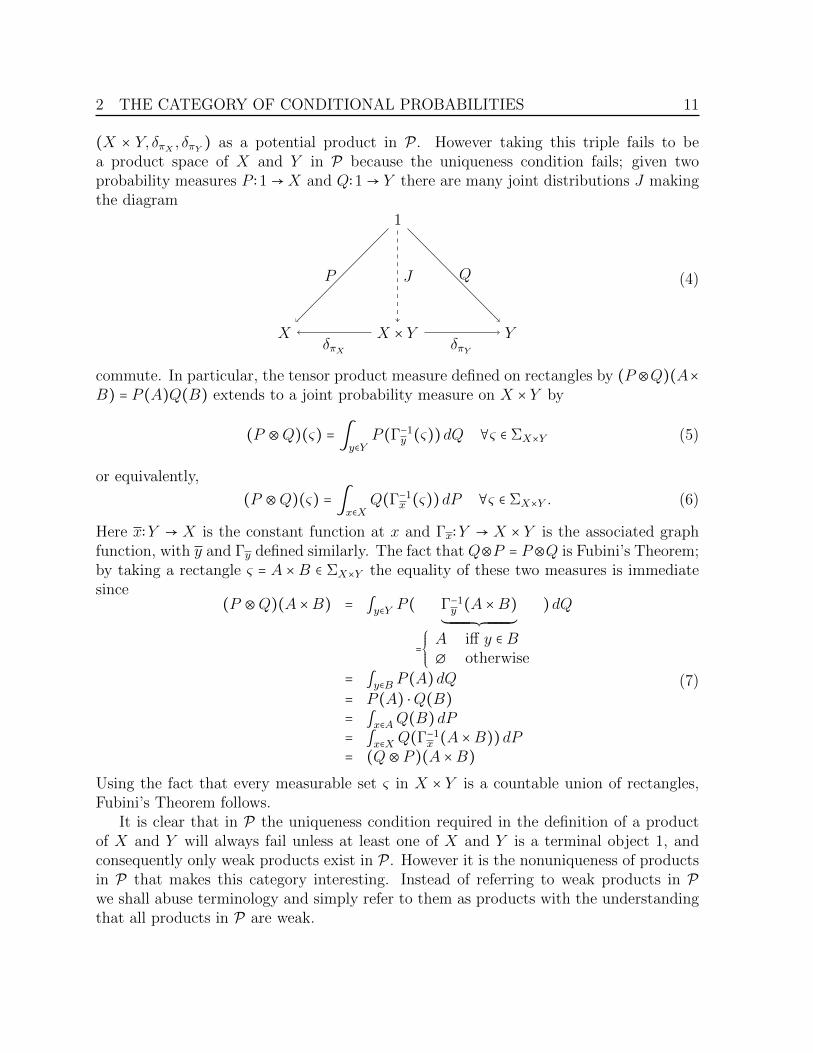
(X × Y, δπX , δπY ) as a potential product in P. However taking this triple fails to bea product space of X and Y in P because the uniqueness condition fails; given twoprobability measures P ∶1→X and Q∶1→ Y there are many joint distributions J makingthe diagram
1
X YX × Y
P QJ
δπX δπY
(4)
commute. In particular, the tensor product measure defined on rectangles by (P ⊗Q)(A×B) = P (A)Q(B) extends to a joint probability measure on X × Y by
(P ⊗Q)(ς) = ∫y∈Y
P (Γ−1y (ς))dQ ∀ς ∈ ΣX×Y (5)
or equivalently,
(P ⊗Q)(ς) = ∫x∈X
Q(Γ−1x (ς))dP ∀ς ∈ ΣX×Y . (6)
Here x∶Y → X is the constant function at x and Γx∶Y → X × Y is the associated graphfunction, with y and Γy defined similarly. The fact that Q⊗P = P⊗Q is Fubini’s Theorem;by taking a rectangle ς = A ×B ∈ ΣX×Y the equality of these two measures is immediatesince
(P ⊗Q)(A ×B) = ∫y∈Y P ( Γ−1y (A ×B)
´¹¹¹¹¹¹¹¹¹¹¹¹¹¹¹¹¹¹¹¹¹¹¹¹¸¹¹¹¹¹¹¹¹¹¹¹¹¹¹¹¹¹¹¹¹¹¹¹¹¹¶=
⎧⎪⎪⎪⎨⎪⎪⎪⎩
A iff y ∈ B∅ otherwise
)dQ
= ∫y∈B P (A)dQ= P (A) ⋅Q(B)= ∫x∈AQ(B)dP= ∫x∈X Q(Γ−1
x (A ×B))dP= (Q⊗ P )(A ×B)
(7)
Using the fact that every measurable set ς in X × Y is a countable union of rectangles,Fubini’s Theorem follows.
It is clear that in P the uniqueness condition required in the definition of a productof X and Y will always fail unless at least one of X and Y is a terminal object 1, andconsequently only weak products exist in P. However it is the nonuniqueness of productsin P that makes this category interesting. Instead of referring to weak products in Pwe shall abuse terminology and simply refer to them as products with the understandingthat all products in P are weak.
2 THE CATEGORY OF CONDITIONAL PROBABILITIES 12
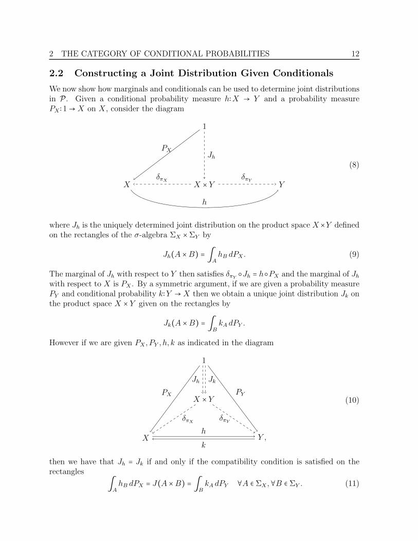
2.2 Constructing a Joint Distribution Given Conditionals
We now show how marginals and conditionals can be used to determine joint distributionsin P. Given a conditional probability measure h∶X → Y and a probability measurePX ∶1→X on X, consider the diagram
1
X YX × Y
PX
δπX δπY
Jh
h
(8)
where Jh is the uniquely determined joint distribution on the product space X×Y definedon the rectangles of the σ-algebra ΣX ×ΣY by
Jh(A ×B) = ∫AhB dPX . (9)
The marginal of Jh with respect to Y then satisfies δπY Jh = hPX and the marginal of Jhwith respect to X is PX . By a symmetric argument, if we are given a probability measurePY and conditional probability k∶Y →X then we obtain a unique joint distribution Jk onthe product space X × Y given on the rectangles by
Jk(A ×B) = ∫BkA dPY .
However if we are given PX , PY , h, k as indicated in the diagram
1
X Y ,
X × YPYPX
δπX δπY
JkJh
h
k
(10)
then we have that Jh = Jk if and only if the compatibility condition is satisfied on therectangles
∫AhB dPX = J(A ×B) = ∫
BkA dPY ∀A ∈ ΣX ,∀B ∈ ΣY . (11)

2 THE CATEGORY OF CONDITIONAL PROBABILITIES 13
In the extreme case, suppose we have a conditional h∶X → Y which factors throughthe terminal object 1 as
X Y
1
h
! Q
where ! represents the unique arrow from X → 1. If we are also given a probability measureP ∶1→X, then we can calculate the joint distribution determined by P and h = Q! as
J(A ×B) = ∫A(Q!)B dP= P (A) ⋅Q(B)
so that J = P ⊗Q. In this situation we say that the marginals P and Q are independent.Thus in P independence corresponds to a special instance of a conditional—one thatfactors through the terminal object.
2.3 Constructing Regular Conditionals given a Joint Distribu-tion
The following result is the theorem from which the inference maps in Bayesian probabil-ity theory are constructed. The fact that we require equiperfect families of probabilitymeasures is critical for the construction.
Theorem 1. Let X and Y be countably generated measurable spaces and (X × Y,ΣX×Y )the product in Meas with projection map πY . If J is a joint distribution on X × Y withmarginal PY = δπY J on Y , then there exists a P arrow f that makes the diagram
1
YX × Y
PYJ
δπY
f
(12)
commute and satisfies
∫A×B
δπY C dJ = ∫CfA×B dPY .
Moreover, this f is the unique P-morphism with these properties, up to a set of PY -measure zero.
Proof. Since ΣX and ΣY are both countably generated, it follows that ΣX×Y is countablygenerated as well. Let G be a countable generating set for ΣX×Y . For each A ∈ G, definea measure µA on Y by
µA(B) = J(A ∩ π−1Y B).
2 THE CATEGORY OF CONDITIONAL PROBABILITIES 14
Then µA is absolutely continuous with respect to PY and hence we can let fA = dµAdPY
, theRadon–Nikodym derivative. For each A ∈ G this Radon–Nikodym derivative is unique upto a set of measure zero, say A. Let N = ∪A∈AA and E1 = N c. Then fA∣E1 is unique forall A ∈ A. Note that fX×Y = 1 and f∅ = 0 on E1. The condition fA ≤ 1 on E1 for all A ∈ Athen follows.
For all B ∈ ΣY and any countable union ∪ni=1Ai of disjoint sets of A we have
∫B∩E1f∪ni=1AidPY = J ((∪ni=1Ai) ∩ π−1
Y B)= ∑n
i=1 J(Ai ∩ π−1Y B)
= ∫B∩E1∑ni=1 fAidPY ,
with the last equality following from the Monotone Convergence Theorem and the factthat all of the fAi are nonnegative. From the uniqueness of the Radon–Nikodym derivativeit follows
f∪ni=1Ai =n
∑i=1
fAi PY -a.e.
Since there exist only a countable number of finite collection of sets of A we can find aset E ⊂ E1 of PY -measure one such that the normalized set function f⋅(y)∶A → [0,1] isfinitely additive on E.
These facts altogether show there exists a set E ∈ ΣY with PY -measure one where forall y ∈ E,
1. 0 ≤ fA(y) ≤ 1 ∀A ∈ A,
2. f∅(y) = 0 and fX×Y (y) = 1, and
3. for any finite collection Aini=1 of disjoint sets of A we have f∪ni=1Ai(y) = ∑ni=1 fAi(y).
Thus the set function f ∶E × A → [0,1] satisfies the condition that f(y, ⋅) is a proba-bility measure on the algebra A. By the Caratheodory extension theorem there exist aunique extension of f(y, ⋅) to a probability measure f(y, ⋅)∶ΣX×Y → [0,1]. Now define aset function f ∶Y ×ΣX×Y → [0,1] by
f(y,A) = f(y,A) if y ∈ EJ(A) if y ∉ E .
Since each A ∈ ΣX×Y can be written as the pointwise limit of an increasing sequenceAn∞n=1 of sets An ∈ A it follows that fA = limn→∞ fAn is measurable. From this we alsoobtain the desired commutativity of the diagram
f PY (A) = ∫Y fAdPY = ∫E fAdPY = limn→∞ ∫E fAndPY= limn→∞ ∫Y fAndPY= limn→∞ J(An)= J(A)
3 THE BAYESIAN PARADIGM USING P 15
We can use the result from Theorem 1 to obtain a broader understanding of thesituation.
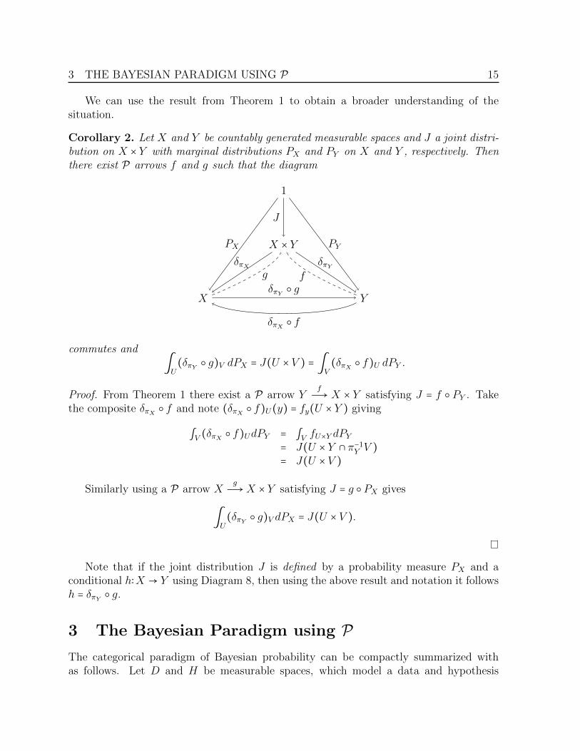
Corollary 2. Let X and Y be countably generated measurable spaces and J a joint distri-bution on X × Y with marginal distributions PX and PY on X and Y , respectively. Thenthere exist P arrows f and g such that the diagram
1
YX
X × Y PYPX
J
δπYδπX
δπX f
fg
δπY g
commutes and
∫U(δπY g)V dPX = J(U × V ) = ∫
V(δπX f)U dPY .
Proof. From Theorem 1 there exist a P arrow YfÐ→ X × Y satisfying J = f PY . Take
the composite δπX f and note (δπX f)U(y) = fy(U × Y ) giving
∫V (δπX f)UdPY = ∫V fU×Y dPY= J(U × Y ∩ π−1
Y V )= J(U × V )
Similarly using a P arrow XgÐ→X × Y satisfying J = g PX gives
∫U(δπY g)V dPX = J(U × V ).
Note that if the joint distribution J is defined by a probability measure PX and aconditional h∶X → Y using Diagram 8, then using the above result and notation it followsh = δπY g.
3 The Bayesian Paradigm using PThe categorical paradigm of Bayesian probability can be compactly summarized withas follows. Let D and H be measurable spaces, which model a data and hypothesis
3 THE BAYESIAN PARADIGM USING P 16
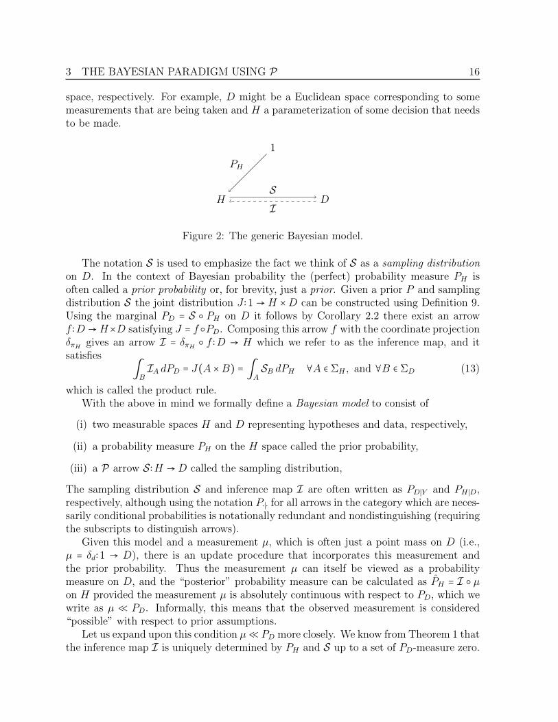
space, respectively. For example, D might be a Euclidean space corresponding to somemeasurements that are being taken and H a parameterization of some decision that needsto be made.
1
H D
PH
SI
Figure 2: The generic Bayesian model.
The notation S is used to emphasize the fact we think of S as a sampling distributionon D. In the context of Bayesian probability the (perfect) probability measure PH isoften called a prior probability or, for brevity, just a prior. Given a prior P and samplingdistribution S the joint distribution J ∶1 → H ×D can be constructed using Definition 9.Using the marginal PD = S PH on D it follows by Corollary 2.2 there exist an arrowf ∶D →H×D satisfying J = f PD. Composing this arrow f with the coordinate projectionδπH gives an arrow I = δπH f ∶D → H which we refer to as the inference map, and itsatisfies
∫BIA dPD = J(A ×B) = ∫
ASB dPH ∀A ∈ ΣH , and ∀B ∈ ΣD (13)
which is called the product rule.With the above in mind we formally define a Bayesian model to consist of
(i) two measurable spaces H and D representing hypotheses and data, respectively,
(ii) a probability measure PH on the H space called the prior probability,
(iii) a P arrow S ∶H →D called the sampling distribution,
The sampling distribution S and inference map I are often written as PD∣Y and PH ∣D,respectively, although using the notation P⋅∣⋅ for all arrows in the category which are neces-sarily conditional probabilities is notationally redundant and nondistinguishing (requiringthe subscripts to distinguish arrows).
Given this model and a measurement µ, which is often just a point mass on D (i.e.,µ = δd∶1 → D), there is an update procedure that incorporates this measurement andthe prior probability. Thus the measurement µ can itself be viewed as a probabilitymeasure on D, and the “posterior” probability measure can be calculated as PH = I µon H provided the measurement µ is absolutely continuous with respect to PD, which wewrite as µ ≪ PD. Informally, this means that the observed measurement is considered“possible” with respect to prior assumptions.
Let us expand upon this condition µ≪ PD more closely. We know from Theorem 1 thatthe inference map I is uniquely determined by PH and S up to a set of PD-measure zero.
3 THE BAYESIAN PARADIGM USING P 17
In general, there is no reason a priori that an arbitrary (perfect) probability measurementµ∶1→D is required to be absolutely continuous with respect to PD. If µ is not absolutelycontinuous with respect to PD, then a different choice of inference map I ′ could yielda different posterior probability—i.e., we could have I µ ≠ I ′ µ. Thus we make theassumption that measurement probabilities on D are absolutely continuous with respectto the prior probability PD on D.
In practice this condition is often not met. For example the probability measure PDmay be a normal distribution on R and consequently PD(y) = 0 for any point y ∈ R.Since Dirac measurements do not satisfy δy ≪ PD, this could create a problem. However,it is clear that the Dirac measures can be approximated arbitrarily closely by a limitingprocess of sharply peaked normal distributions which do satisfy this absolute continuitycondition. Thus while the absolute continuity condition may not be satisfied precisely theerror in approximating the measurement by assuming a Dirac measure is negligible. Thusit is standard to assume that measurements belong to a particular class of probabilitymeasures on D which are broad enough to approximate measurements and known to beabsolutely continuous with respect to the prior.
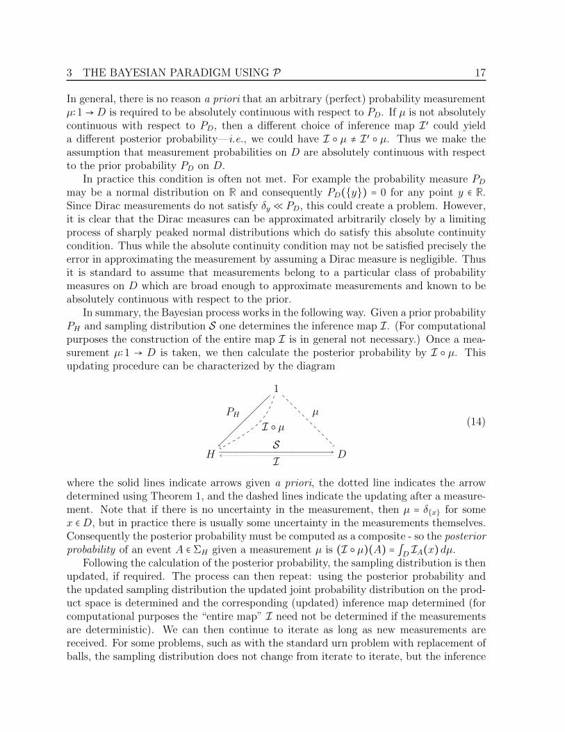
In summary, the Bayesian process works in the following way. Given a prior probabilityPH and sampling distribution S one determines the inference map I. (For computationalpurposes the construction of the entire map I is in general not necessary.) Once a mea-surement µ∶1 → D is taken, we then calculate the posterior probability by I µ. Thisupdating procedure can be characterized by the diagram
1
H D
PH µ
SI
I µ (14)
where the solid lines indicate arrows given a priori, the dotted line indicates the arrowdetermined using Theorem 1, and the dashed lines indicate the updating after a measure-ment. Note that if there is no uncertainty in the measurement, then µ = δx for somex ∈D, but in practice there is usually some uncertainty in the measurements themselves.Consequently the posterior probability must be computed as a composite - so the posteriorprobability of an event A ∈ ΣH given a measurement µ is (I µ)(A) = ∫D IA(x)dµ.
Following the calculation of the posterior probability, the sampling distribution is thenupdated, if required. The process can then repeat: using the posterior probability andthe updated sampling distribution the updated joint probability distribution on the prod-uct space is determined and the corresponding (updated) inference map determined (forcomputational purposes the “entire map” I need not be determined if the measurementsare deterministic). We can then continue to iterate as long as new measurements arereceived. For some problems, such as with the standard urn problem with replacement ofballs, the sampling distribution does not change from iterate to iterate, but the inference

4 ELEMENTARY APPLICATIONS OF BAYESIAN PROBABILITY 18
map is updated since the posterior probability on the hypothesis space changes with eachmeasurement.
Remark 3. Note that for countable spaces X and Y the compatibility condition reduces tothe standard Bayes equation since for any x ∈X the singleton x ∈ ΣX and similarly anyelement y ∈ Y implies y ∈ ΣY , so that the joint distribution J ∶1 → X × Y on x × yreduces to the equation
S(y ∣ x)PX(x) = J(x × y) = I(x ∣ y)PY (y) (15)
which in more familiar notation is the Bayesian equation
P (y ∣ x)P (x) = P (x, y) = P (x ∣ y)P (y). (16)
4 Elementary applications of Bayesian probability
Before proceeding to show how the category P can be can be applied to ML where theunknowns are functions, we illustrate its use to solve inference, prediction, and decisionprocesses in the more familiar setting where the unknown parameter(s) are real values.We present two elementary problems illustrating basic model building using categoricaldiagrams, much like that used in probabilistic graphical models for Bayesian networks,which can serve to clarify the modeling aspect of any probabilistic problem.
To illustrate the inference-sampling distribution relationship and how we make com-putations in the category P, we consider first an urn problem where we have discreteσ-algebras. The discreteness condition is not critical as we will eventually see - it onlymakes the analysis and computational aspect easier.
Example 4. Million dollar draw.11
R B R
B R
Urn 1 Urn 2
R B B
B
You are given two draws and if you pull out a red ball you win a million dollars. Youare unable to see the two urns so you don’t know which urn you are drawing from andthe draw is done without replacement. The P diagram for both inference and calculatingsampling distributions is given by
11 This problem is taken from Peter Green’s tutorial on Bayesian Inference which can be viewed athttp://videolectures.net/mlss2011 green bayesian.

4 ELEMENTARY APPLICATIONS OF BAYESIAN PROBABILITY 19
1
U B
PU
SI
PB
where the dashed arrows indicate morphisms to be calculated rather than morphismsdetermined by modeling,
U = u1, u2 = Urn 1, Urn 2B = b, r = blue, red
and
PU = 1
2δu1 +
1
2δu2 .
The sampling distribution is the binomial distribution given by
S(b ∣ u1) = 25 S(r ∣ u1) = 3
5
S(b ∣ u2) = 34 S(r ∣ u2) = 1
4 .
Suppose that on our first draw, we draw from one of the urns (which one is unknown)and draw a blue ball. We ask the following questions:
1. (Inference) What is the probability that we made the draw from Urn 1 (Urn 2)?
2. (Prediction) What is the probability of drawing a red ball on the second draw (fromthe same urn)?
3. (Decision) Given you have drawn a blue ball on the first draw should you switchurns to increase the probability of drawing a red ball?
To solve these problems, we implicitly or explicitly construct the joint distribution Jvia the standard construction given PU and the conditional S
1
U BU ×B
PB = S PU
δπB
PU
δπU
J
S
4 ELEMENTARY APPLICATIONS OF BAYESIAN PROBABILITY 20
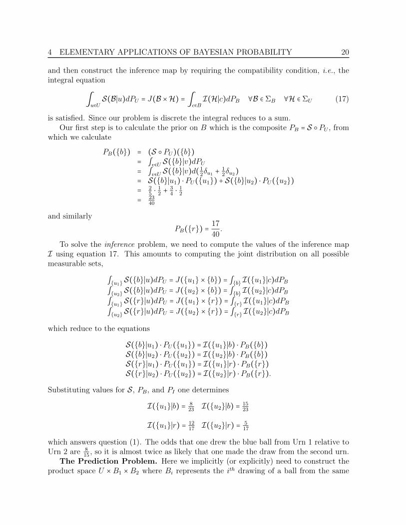
and then construct the inference map by requiring the compatibility condition, i.e., theintegral equation
∫u∈US(B∣u)dPU = J(B ×H) = ∫
c∈BI(H∣c)dPB ∀B ∈ ΣB ∀H ∈ ΣU (17)
is satisfied. Since our problem is discrete the integral reduces to a sum.Our first step is to calculate the prior on B which is the composite PB = S PU , from
which we calculate
PB(b) = (S PU)(b)= ∫v∈U S(b∣v)dPU= ∫v∈U S(b∣v)d(1
2δu1 + 12δu2)
= S(b∣u1) ⋅ PU(u1) + S(b∣u2) ⋅ PU(u2)= 2
5 ⋅ 12 + 3
4 ⋅ 12
= 2340
and similarly
PB(r) =17
40.
To solve the inference problem, we need to compute the values of the inference mapI using equation 17. This amounts to computing the joint distribution on all possiblemeasurable sets,
∫u1 S(b∣u)dPU = J(u1 × b) = ∫b I(u1∣c)dPB∫u2 S(b∣u)dPU = J(u2 × b) = ∫b I(u2∣c)dPB∫u1 S(r∣u)dPU = J(u1 × r) = ∫r I(u1∣c)dPB∫u2 S(r∣u)dPU = J(u2 × r) = ∫r I(u2∣c)dPB
which reduce to the equations
S(b∣u1) ⋅ PU(u1) = I(u1∣b) ⋅ PB(b)S(b∣u2) ⋅ PU(u2) = I(u2∣b) ⋅ PB(b)S(r∣u1) ⋅ PU(u1) = I(u1∣r) ⋅ PB(r)S(r∣u2) ⋅ PU(u2) = I(u2∣r) ⋅ PB(r).
Substituting values for S, PB, and PI one determines
I(u1∣b) = 823 I(u2∣b) = 15
23
I(u1∣r) = 1217 I(u2∣r) = 5
17
which answers question (1). The odds that one drew the blue ball from Urn 1 relative toUrn 2 are 8
15 , so it is almost twice as likely that one made the draw from the second urn.The Prediction Problem. Here we implicitly (or explicitly) need to construct the
product space U ×B1 ×B2 where Bi represents the ith drawing of a ball from the same
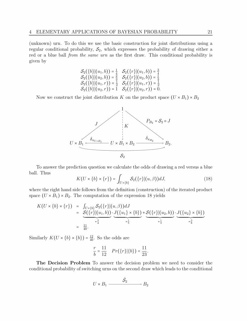
4 ELEMENTARY APPLICATIONS OF BAYESIAN PROBABILITY 21
(unknown) urn. To do this we use the basic construction for joint distributions using aregular conditional probability, S2, which expresses the probability of drawing either ared or a blue ball from the same urn as the first draw. This conditional probability isgiven by
S2(b∣(u1, b)) = 14 S2(r∣(u1, b)) = 3
4
S2(b∣(u2, b)) = 23 S2(r∣(u2, b)) = 1
3
S2(b∣(u1, r)) = 12 S2(r∣(u1, r)) = 1
2
S2(b∣(u2, r)) = 1 S2(r∣(u2, r)) = 0.
Now we construct the joint distribution K on the product space (U ×B1) ×B2
1
U ×B1 B2.U ×B1 ×B2
PB2 = S2 J
δπB2
J
δπU×B1
K
S2
To answer the prediction question we calculate the odds of drawing a red versus a blueball. Thus
K(U × b × r) = ∫U×b
S2(r∣(u,β))dJ, (18)
where the right hand side follows from the definition (construction) of the iterated productspace (U ×B1) ×B2. The computation of the expression 18 yields
K(U × b × r) = ∫U×b S2(r∣(u,β))dJ= S(r∣(u1, b))
´¹¹¹¹¹¹¹¹¹¹¹¹¹¹¹¹¹¹¹¹¹¹¹¹¹¹¹¹¹¹¹¹¹¹¸¹¹¹¹¹¹¹¹¹¹¹¹¹¹¹¹¹¹¹¹¹¹¹¹¹¹¹¹¹¹¹¹¹¹¹¶= 34
⋅J(u1 × b)´¹¹¹¹¹¹¹¹¹¹¹¹¹¹¹¹¹¹¹¹¹¹¹¹¹¹¹¹¹¹¹¹¹¹¸¹¹¹¹¹¹¹¹¹¹¹¹¹¹¹¹¹¹¹¹¹¹¹¹¹¹¹¹¹¹¹¹¹¹
= 15
+S(r∣(u2, b))´¹¹¹¹¹¹¹¹¹¹¹¹¹¹¹¹¹¹¹¹¹¹¹¹¹¹¹¹¹¹¹¹¹¹¸¹¹¹¹¹¹¹¹¹¹¹¹¹¹¹¹¹¹¹¹¹¹¹¹¹¹¹¹¹¹¹¹¹¹¹
= 13
⋅J(u2 × b)´¹¹¹¹¹¹¹¹¹¹¹¹¹¹¹¹¹¹¹¹¹¹¹¹¹¹¹¹¹¹¹¹¹¹¸¹¹¹¹¹¹¹¹¹¹¹¹¹¹¹¹¹¹¹¹¹¹¹¹¹¹¹¹¹¹¹¹¹¹
= 38
= 1140 .
Similarly K(U × b × b) = 1240 . So the odds are
r
b= 11
12Pr(r∣b) = 11
23.
The Decision Problem To answer the decision problem we need to consider theconditional probability of switching urns on the second draw which leads to the conditional
U ×B1 B2
S2

4 ELEMENTARY APPLICATIONS OF BAYESIAN PROBABILITY 22
given byS2(b∣(u1, b)) = 3
4 S2(r∣(u1, b)) = 14
S2(b∣(u2, b)) = 25 S2(r∣(u2, b)) = 3
5
S2(b∣(u1, r)) = 34 S2(r∣(u1, r)) = 1
4
S2(b∣(u2, r)) = 25 S2(r∣(u2, r)) = 3
5 .
Carrying out the same computation as above we find the joint distribution K on theproduct space (U ×B1) ×B2 constructed from J and S2 yields
K(U × b × r) = ∫U×b S2(r∣(u,β))dJ= S2(r∣(u1, b))J(u1 × b) + S2(r∣(u2, b))J(u2 × b)= 1
4 ⋅ 15 + 3
5 ⋅ 38
= 1140 ,
which shows that it doesn’t matter whether you switch or not - you get the same proba-bility of drawing a red ball.
The probability of drawing a blue ball is
K(U × b × b) = 12
40=K(U × b × b),
so the odds of drawing a blue ball outweigh the odds of drawing a red ball by the ratio1211 . The odds are against you.
Here is an example illustrating that the regular conditional probabilities (inference orsampling distributions) are defined only up to sets of measure zero.
Example 5. We have a rather bland deck of three cards as shown
Card 1 Card 2 Card 3
Front
Back
R
R
R
G
G
G
We shuffle the deck, pull out a card and expose one face which is red.12 The predictionquestion is
12 This problem is taken from David MacKays tutorial on Information Theory which can be viewedat http ∶ //videolectures.net/mlss09uk mackay it/.
4 ELEMENTARY APPLICATIONS OF BAYESIAN PROBABILITY 23
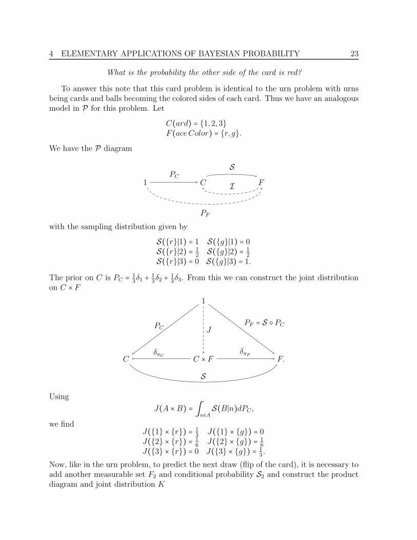
What is the probability the other side of the card is red?
To answer this note that this card problem is identical to the urn problem with urnsbeing cards and balls becoming the colored sides of each card. Thus we have an analogousmodel in P for this problem. Let
C(ard) = 1,2,3F (aceColor) = r, g.
We have the P diagram
1 C FPC
S
I
PF
with the sampling distribution given by
S(r∣1) = 1 S(g∣1) = 0S(r∣2) = 1
2 S(g∣2) = 12
S(r∣3) = 0 S(g∣3) = 1.
The prior on C is PC = 13δ1 + 1
3δ2 + 13δ3. From this we can construct the joint distribution
on C × F1
C F.C × F
PF = S PC
δπF
PC
δπC
J
S
Using
J(A ×B) = ∫n∈AS(B∣n)dPC ,
we findJ(1 × r) = 1
3 J(1 × g) = 0J(2 × r) = 1
6 J(2 × g) = 16
J(3 × r) = 0 J(3 × g) = 13 .
Now, like in the urn problem, to predict the next draw (flip of the card), it is necessary toadd another measurable set F2 and conditional probability S2 and construct the productdiagram and joint distribution K

4 ELEMENTARY APPLICATIONS OF BAYESIAN PROBABILITY 24
1
C × F1 F2.C × F1 × F2
PF2 = S2 J
δπF2
J
δπC×F1
K
S2
The twist now arises in that the conditional probability S2 is not uniquely defined - whatare the values
S2(r∣(1, g)) = ? S2(g∣(1, g)) = ?
The answer is it doesn’t matter what we put down for these values since they have measureJ(1 × g) = 0. We can still compute the desired quantity of interest proceeding forthwith these arbitrarily chosen values on the point sets of measure zero. Thus we choose
S2(g∣(1, r)) = 0 S2(r∣(1, r)) = 1S2(g∣(1, g)) = 1 S2(r∣(1, g)) = 0 doesn’t matterS2(g∣(2, r)) = 1 S2(r∣(2, r)) = 0S2(g∣(2, g)) = 0 S2(r∣(2, g)) = 1S2(g∣(3, r)) = 0 S2(r∣(3, r)) = 1 doesn’t matterS2(g∣(3, g)) = 1 S2(r∣(3, g)) = 0.
We chose the arbitrary values such that S2 is a deterministic mapping which seems ap-propriate since flipping a given card uniquely determined the color on the other side.
Now we can solve the prediction problem by computing the joint measure values
K(C × r × r) = ∫C×r(S2)r(n, c)dJ= S2(r∣(1, r)) ⋅ J(1 × r) + S2(r∣(2, r)) ⋅ J(2 × r)= 1 ⋅ 1
3 + 0 ⋅ 16
= 13
and
K(C × r × g) = ∫C×r S2(g∣(n, c))dJ= S2(g∣(1, r)) ⋅ J(1 × r) + S2(g∣(2, r)) ⋅ J(2 × r)= 0 ⋅ 1
3 + 1 ⋅ 16
= 16 ,
so it is twice as likely to observe a red face upon flipping the card than seeing a greenface. Converting the odds of r
g = 21 to a probability gives Pr(r∣r) = 2
3 .
To test one’s understanding of the categorical approach to Bayesian probability wesuggest the following problem.
5 THE TENSOR PRODUCT 25
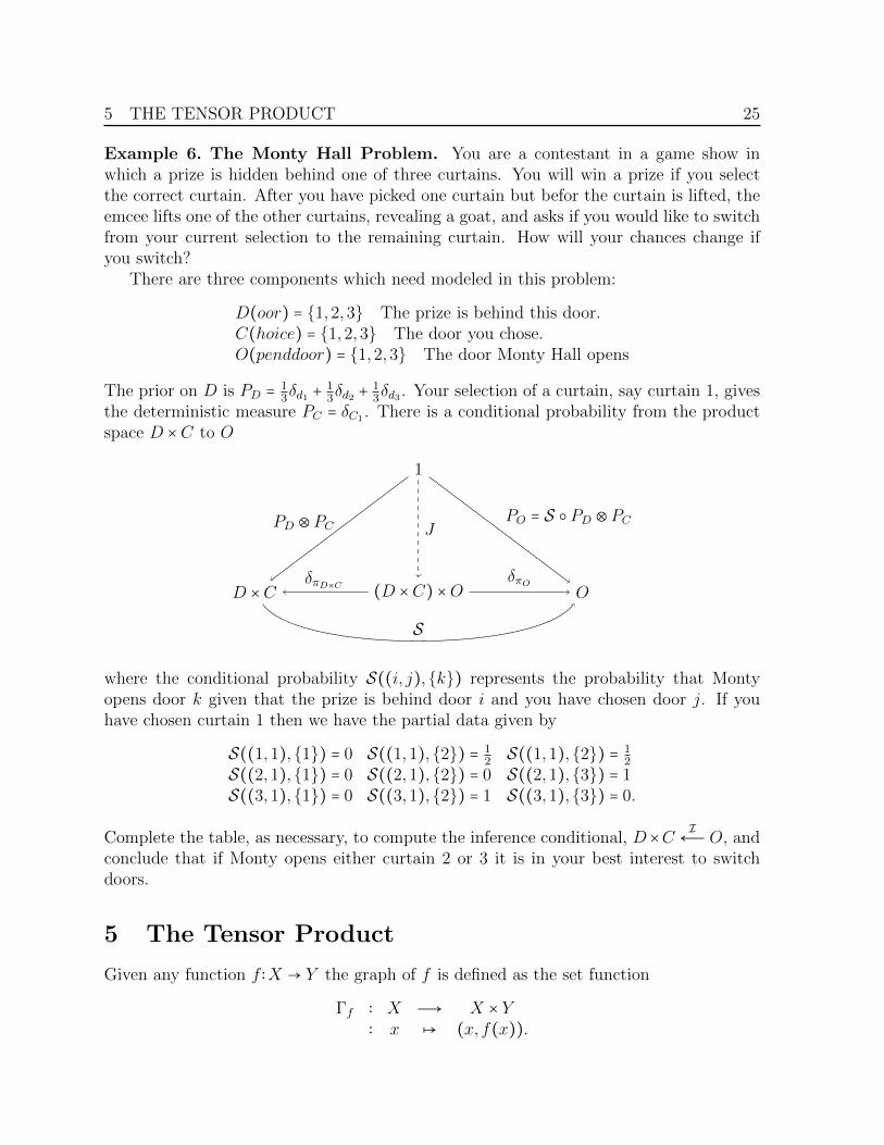
Example 6. The Monty Hall Problem. You are a contestant in a game show inwhich a prize is hidden behind one of three curtains. You will win a prize if you selectthe correct curtain. After you have picked one curtain but befor the curtain is lifted, theemcee lifts one of the other curtains, revealing a goat, and asks if you would like to switchfrom your current selection to the remaining curtain. How will your chances change ifyou switch?
There are three components which need modeled in this problem:
D(oor) = 1,2,3 The prize is behind this door.C(hoice) = 1,2,3 The door you chose.O(penddoor) = 1,2,3 The door Monty Hall opens
The prior on D is PD = 13δd1 + 1
3δd2 + 13δd3 . Your selection of a curtain, say curtain 1, gives
the deterministic measure PC = δC1 . There is a conditional probability from the productspace D ×C to O
1
D ×C O(D ×C) ×O
PO = S PD ⊗ PC
δπO
PD ⊗ PC
δπD×C
J
S
where the conditional probability S((i, j),k) represents the probability that Montyopens door k given that the prize is behind door i and you have chosen door j. If youhave chosen curtain 1 then we have the partial data given by
S((1,1),1) = 0 S((1,1),2) = 12 S((1,1),2) = 1
2
S((2,1),1) = 0 S((2,1),2) = 0 S((2,1),3) = 1S((3,1),1) = 0 S((3,1),2) = 1 S((3,1),3) = 0.
Complete the table, as necessary, to compute the inference conditional, D×C I←Ð O, andconclude that if Monty opens either curtain 2 or 3 it is in your best interest to switchdoors.
5 The Tensor Product
Given any function f ∶X → Y the graph of f is defined as the set function
Γf ∶ X Ð→ X × Y∶ x ↦ (x, f(x)).

5 THE TENSOR PRODUCT 26
By our previous notation Γf = ⟨IdX , f⟩. If g∶Y → X is any function we also refer to theset function
Γg ∶ Y Ð→ X × Y∶ y ↦ (g(y), y)
as a graph function.Any fixed x ∈ X determines a constant function x∶Y → X sending every y ∈ Y to
x. These functions are always measurable and consequently determine “constant” graphfunctions Γx∶Y →X×Y . Similarly, every fixed y ∈ Y determines a constant graph functionΓy ∶X →X×Y . Together, these constant graph functions can be used to define a σ-algebraon the set X × Y which is finer (larger) than the product σ-algebra ΣX×Y . Let X ⊗ Ydenote the set X × Y endowed with the largest σ-algebra structure such that all theconstant graph functions Γx∶X →X ⊗Y and Γy ∶Y →X ⊗Y are measurable. We say thisσ-algebra X ⊗ Y is coinduced by the maps Γx∶X →X × Y x∈X and Γy ∶Y →X × Y y∈Y .Explicitly, this σ-algebra is given by
ΣX⊗Y = ⋂x∈X
Γx∗ΣY ∩ ⋂y∈Y
Γy∗ΣX , (19)
where for any function f ∶W → Z,
f∗ΣW = C ∈ 2Z ∣ f−1(C) ∈ ΣW. (20)
This is in contrast to the smallest σ-algebra on X × Y , defined in Section 2.1 so that thetwo projection maps πX ∶X ×Y →X,πY ∶X ×Y → Y are measurable. Such a σ-algebra issaid to be induced by the projection maps, or simply referred to as the initial σ-algebra.
The following result on coinduced σ-algebras is used repeatedly.
Lemma 7. Let the σ-algebra of Y be coinduced by a collection of maps fi∶Xi → Y i∈I .Then any map g∶Y → Z is measurable if and only if the composition g fi is measurablefor each i ∈ I.
Proof. Consider the diagram
Xi Y
Z
fi
gg fi
If B ∈ ΣZ then g−1(B) ∈ ΣY if and only if f−1i (g−1(B)) ∈ ΣX .
This result is used frequently when Y in the above diagram is replaced by a tensorproduct space X ⊗ Y . For example, using this lemma it follows that the projection maps

5 THE TENSOR PRODUCT 27
πY ∶X⊗Y → Y and πX ∶X⊗Y →X are both measurable because the diagrams in Figure 3commute.
X
YX ⊗ Y
yΓy
πY
Y
X X ⊗ Y
x Γx
πX
Figure 3: The commutativity of these diagrams, together with the measurability of theconstant functions and constant graph functions, implies the projection maps πX and πYare measurable.
By the measurability of the projection maps and the universal property of the product,it follows the identity mapping on the set X × Y yields a measurable function
X ⊗ Y X × Yid
called the restriction of the σ-algebra. In contrast, the identity function X × Y → X ⊗ Yis not necessarily measurable. Given any probability measure P on X ⊗Y the restrictionmapping induces the pushforward probability measure δid P = P (id−1(⋅)) on the productσ-algebra.
5.1 Graphs of Conditional Probabilities
The tensor product of two probability measures P ∶1 → X and Q∶1 → Y was defined inEquations 5 and 6 as the joint distribution on the product σ-algebra by either of theexpressions
(P⋉Q)(ς) = ∫y∈Y
P (Γ−1y (ς))dQ ∀ς ∈ ΣX×Y
and(P⋊Q)(ς) = ∫
x∈XQ(Γ−1
x (ς))dP ∀ς ∈ ΣX×Y
which are equivalent on the product σ-algebra. Here we have introduced the new notationof left tensor ⋉ and right tensor ⋊ because we can extend these definitions to be definedon the tensor σ-algebra though in general the equivalence of these two expressions may nolonger hold true. These definitions can be extended to conditional probability measuresP ∶Z →X and Q∶Z → Y trivially by conditioning on a point z ∈ Z,
(P⋉Q)(ς ∣ z) = ∫y∈Y
P (Γ−1y (ς))dQz ∀ς ∈ ΣX⊗Y (21)

5 THE TENSOR PRODUCT 28
and(P⋊Q)(ς ∣ z) = ∫
x∈XQ(Γ−1
x (ς))dPz ∀ς ∈ ΣX⊗Y (22)
which are equivalent on the product σ-algebra but not on the tensor σ-algebra. Howeverin the special case when Z = X and P = 1X , then Equations 21 and 22 do coincide onΣX⊗Y because by Equation 21
(1X⋉Q)(ς ∣ x) = ∫y∈Y δx(Γ−1y (ς))
´¹¹¹¹¹¹¹¹¹¹¹¹¹¹¹¹¹¹¹¹¹¸¹¹¹¹¹¹¹¹¹¹¹¹¹¹¹¹¹¹¹¹¹¹¶=
⎧⎪⎪⎪⎨⎪⎪⎪⎩
1 iff (x, y) ∈ ς0 otherwise
dQx ∀ς ∈ ΣX⊗Y X
= ∫y∈Y χΓ−1x
(ς)(y)dQx
= Qx(Γ−1x (ς)),
(23)
while by Equation 22
(1X⋊Q)(ς ∣ x) = ∫u∈X Qx(Γ−1u (ς))d (δIdX)x
´¹¹¹¹¹¹¹¹¹¸¹¹¹¹¹¹¹¹¹¶=δx
∀ς ∈ ΣX⊗Y X
= Qx(Γ−1x (U)).
(24)
In this case we denote the common conditional by ΓQ, called the graph of Q by analogyto the graph of a function, and this map gives the commutative diagram in Figure 4.
X
X YX ⊗ Y
1X QΓQ
δπX δπY
Figure 4: The tensor product of a conditional with an identity map in P.
The commutativity of the diagram in Figure 4 follows from
(δπX ΓQ)(A ∣ x) = ∫(u,v)∈X⊗Y δπX(A ∣ (u, v))d (ΓQ)x²=QΓ−1
x
= ∫v∈Y δπX(A ∣ Γx(v))dQx
= ∫v∈Y δx(A)dQx
= δx(A) ∫Y dQx
= 1X(A ∣ x)
(25)
5 THE TENSOR PRODUCT 29
and(δπY ΓQ)(B ∣ x) = ∫(u,v)∈X⊗Y δπY (B ∣ (u, v))d((ΓQ)x)
= ∫v∈Y δπY (B ∣ (x, v))dQx
= ∫v∈Y χB(v)dQx
= Q(A ∣ x).
(26)
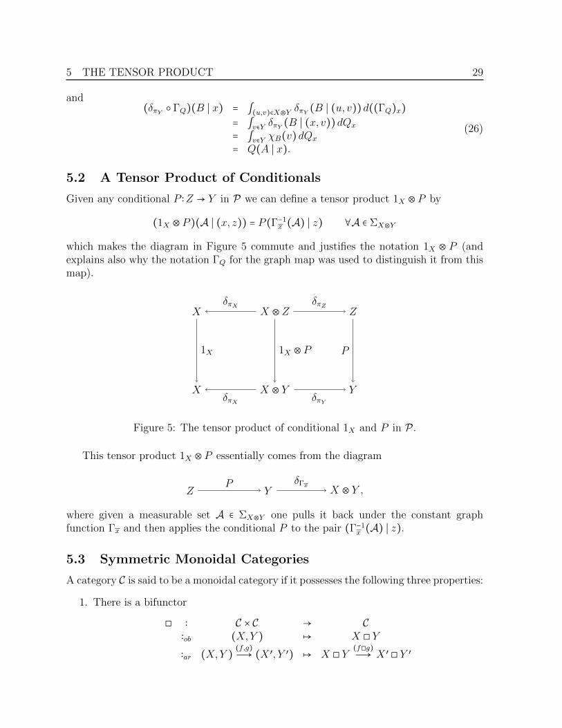
5.2 A Tensor Product of Conditionals
Given any conditional P ∶Z → Y in P we can define a tensor product 1X ⊗ P by
(1X ⊗ P )(A ∣ (x, z)) = P (Γ−1x (A) ∣ z) ∀A ∈ ΣX⊗Y
which makes the diagram in Figure 5 commute and justifies the notation 1X ⊗ P (andexplains also why the notation ΓQ for the graph map was used to distinguish it from thismap).
X ⊗ZX Z
X ⊗ YX Y
1X ⊗ P
δπX δπZ
δπX δπY
1X P
Figure 5: The tensor product of conditional 1X and P in P.
This tensor product 1X ⊗ P essentially comes from the diagram
Z Y X ⊗ Y ,P δΓx
where given a measurable set A ∈ ΣX⊗Y one pulls it back under the constant graphfunction Γx and then applies the conditional P to the pair (Γ−1
x (A) ∣ z).
5.3 Symmetric Monoidal Categories
A category C is said to be a monoidal category if it possesses the following three properties:
1. There is a bifunctor
◻ ∶ C × C → C∶ob (X,Y ) ↦ X ◻ Y∶ar (X,Y ) (f,g)Ð→ (X ′, Y ′) ↦ X ◻ Y (f◻g)Ð→ X ′ ◻ Y ′
5 THE TENSOR PRODUCT 30
which is associative up to isomorphism,
◻ (◻ × IdC) ≅ ◻(IdC × ◻)∶C × C × C → C
where IdC is the identity functor on C. Hence for every triple X,Y,Z of objects,there is an isomorphism
aX,Y,Z ∶ (X ◻ Y ) ◻Z Ð→X ◻ (Y ◻Z)
which is natural in X,Y,Z. This condition is called the associativity axiom.
2. There is an object I ∈ C such that for every object X ∈ob C there is a left unitisomorphism
lX ∶1 ◻X Ð→X.
and a right unit isomorphism
rX ∶X ◻ 1Ð→X.
These two conditions are called the unity axioms.
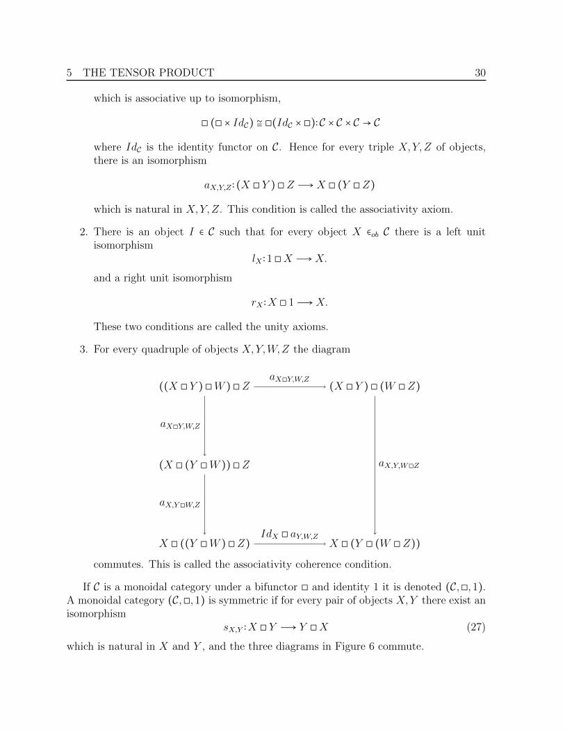
3. For every quadruple of objects X,Y,W,Z the diagram
((X ◻ Y ) ◻W ) ◻Z
(X ◻ (Y ◻W )) ◻Z
X ◻ ((Y ◻W ) ◻Z)
(X ◻ Y ) ◻ (W ◻Z)
X ◻ (Y ◻ (W ◻Z))
aX◻Y,W,Z
IdX ◻ aY,W,Z
aX,Y,W◻Z
aX◻Y,W,Z
aX,Y ◻W,Z
commutes. This is called the associativity coherence condition.
If C is a monoidal category under a bifunctor ◻ and identity 1 it is denoted (C,◻,1).A monoidal category (C,◻,1) is symmetric if for every pair of objects X,Y there exist anisomorphism
sX,Y ∶X ◻ Y Ð→ Y ◻X (27)
which is natural in X and Y , and the three diagrams in Figure 6 commute.

6 FUNCTION SPACES 31
(X ◻ Y ) ◻Z
X ◻ (Y ◻Z)
Y ◻ (Z ◻X)
(Y ◻X) ◻Z
Y ◻ (X ◻Z)
Y ◻ (Z ◻X)
sX,Y ◻ IdZ
aY,Z,X
aY,X,ZaX,Y,Z
sX,Y ◻Z IdY ⊗ sX,Z
X ◻ I I ◻X
X
sX,1
rX lX
X ◻ Y Y ◻X
X ◻ Y
sX,Y
sY,X IdX
Figure 6: The additional conditions required for a symmetric monoidal category.
The main example of a symmetric monoidal category is the category of sets, Set,under the cartesian product with identity the terminal object 1 = ⋆. Similarly, for thecategories Meas and P, the tensor product ⊗ along with the terminal object 1 acting asthe identity element make both (Meas,⊗,1) and (P,⊗,1) symmetric monoidal categorieswith the above conditions straightforward to verify. This provides a good exercise for thereader new to categorical methods.
6 Function Spaces
For X,Y ∈obMeas let Y X denote the set of all measurable functions from X to Y endowedwith the σ-algebra induced by the set of all point evaluation maps evxx∈X , where
Y X evxÐ→ Yf ↦ f(x).
Explicitly, the σ-algebra on Y X is given by
ΣY X = σ (⋃x∈X
ev−1x ΣY ) , (28)
where for any function f ∶W → Z we have
f−1ΣZ = B ∈ 2W ∣ ∃C ∈ ΣZ with f−1(C) = B (29)
and σ(B) denotes the σ-algebra generated by any collection B of subsets.

6 FUNCTION SPACES 32
Formally we should use an alternative notation such as f to distinguish betweenthe measurable function f ∶X → Y and the point f∶1→ Y X of the function space Y X .13
However, it is common practice to let the context define which arrow we are referring toand we shall often follow this practice unless the distinction is critical to avoid ambiguityor awkward expressions.
An alternative notation to Y X is ∏x∈X Yx where each Yx is a copy of Y . The relation-ship between these representations is that in the former we view the elements as functionsf while in the latter we view the elements as the indexed images of a function, f(x)x∈X .Either representation determines the other since a function is uniquely specified by itsvalues.
Because the σ-algebra structure on tensor product spaces was defined precisely so thatthe constant graph functions were all measurable, it follows that in particular the constantgraph functions Γf ∶X →X ⊗Y X sending x↦ (x, f) are measurable. (The graph functionsymbol Γ⋅ is overloaded and will need to be specified directly (domain and codomain)when the context is not clear.)
Define the evaluation function
X ⊗ Y XevX,YÐ→ Y
(x, f) ↦ f(x) (30)
and observe that for every f ∈ Y X the right handMeas diagram in Figure 7 is commu-tative as a set mapping, f = evX,Y Γf .
X ≅X ⊗ 1
X ⊗ Y X Y
1
Y X
Γf ≅ IdX ⊗ f f
evX,Y
f
Figure 7: The defining characteristic property of the evaluation function ev for graphs.
By rotating the diagram in Figure 7 and also considering the constant graph functionsΓx, the right hand side of the diagram in Figure 8 also commutes for every x ∈X.
13Having defined Y X to be the set of all measurable functions f ∶X → Y it seems contradictory to thendefine evx as acting on “points” f∶1 → Y X rather than the functions f themselves! The apparent selfcontradictory definition arises because we are interspersing categorical language with set theory; whendefining a set function, like evx, it is implied that it acts on points which are defined as “global elements”1→ Y X . A global element is a map with domain 1. This is the categorical way of defining points ratherthan using the elementhood operator “∈”. Thus, to be more formal, we could have defined evx, wherex∶1→X is any global element, by evx f = f(x)∶1→ Y , where f(x) = f x.
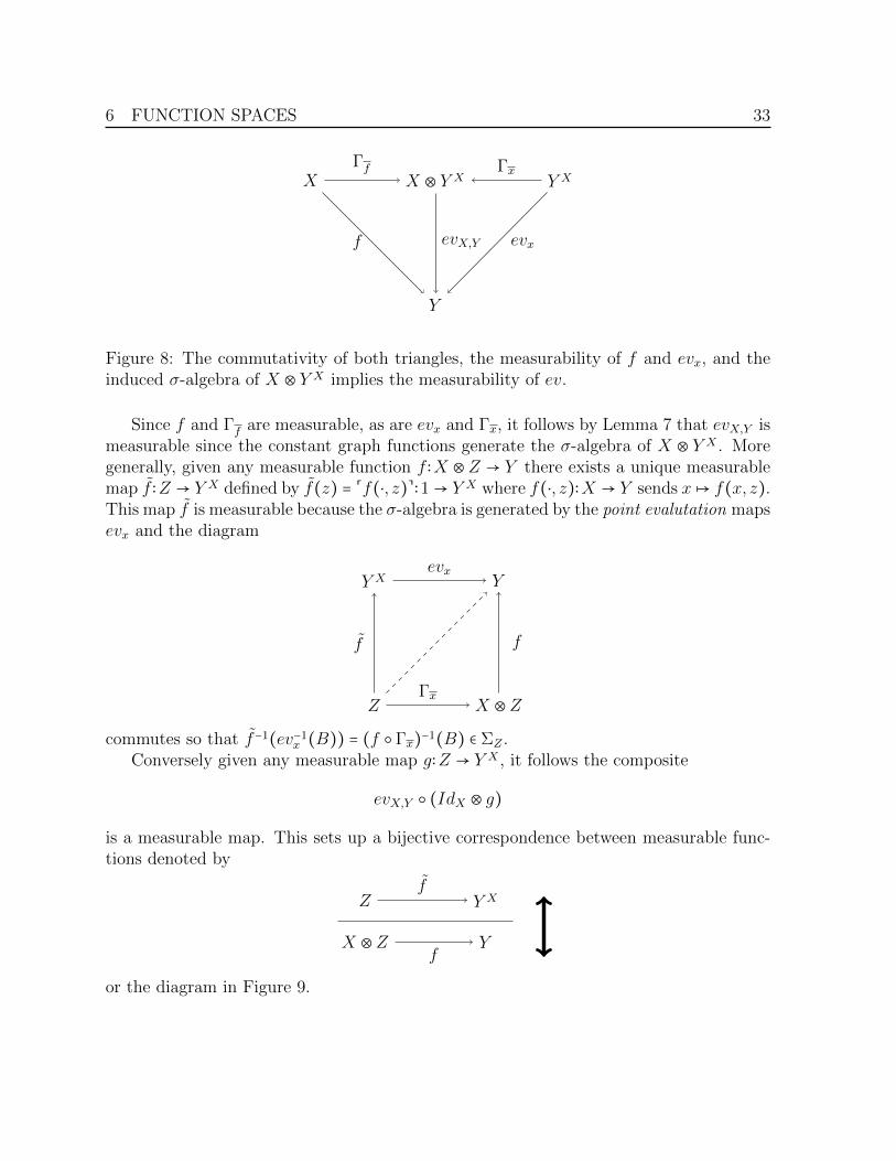
6 FUNCTION SPACES 33
X Y XX ⊗ Y X
Y
Γf
f
Γx
evxevX,Y
Figure 8: The commutativity of both triangles, the measurability of f and evx, and theinduced σ-algebra of X ⊗ Y X implies the measurability of ev.
Since f and Γf are measurable, as are evx and Γx, it follows by Lemma 7 that evX,Y ismeasurable since the constant graph functions generate the σ-algebra of X ⊗ Y X . Moregenerally, given any measurable function f ∶X ⊗Z → Y there exists a unique measurablemap f ∶Z → Y X defined by f(z) = f(⋅, z)∶1→ Y X where f(⋅, z)∶X → Y sends x↦ f(x, z).This map f is measurable because the σ-algebra is generated by the point evalutation mapsevx and the diagram
X ⊗Z
Y X Y
Z
evx
f
Γx
f
commutes so that f−1(ev−1x (B)) = (f Γx)−1(B) ∈ ΣZ .
Conversely given any measurable map g∶Z → Y X , it follows the composite
evX,Y (IdX ⊗ g)
is a measurable map. This sets up a bijective correspondence between measurable func-tions denoted by
Z Y X
X ⊗Z Y
f
f
or the diagram in Figure 9.

6 FUNCTION SPACES 34
X ⊗Z
X ⊗ Y X Y
Z
Y X
IdX ⊗ f f
evX,Y
f
Figure 9: The evaluation function ev sets up a bijective correspondence between the twomeasurable maps f and f .
The measurable map f is called the adjunct of f and vice versa, so that ˜f = f . Whetherwe use the tilde notation for the map X ⊗ Z → Y or the map Z → Y X is irrelevant, itsimply indicates it’s the map uniquely determined by the other map.
The map evX,Y , which we will usually abbreviate to simply ev with the pair (X,Y )obvious from context, is called a universal arrow because of this property; it mediates therelationship between the two maps f and f . In the language of category theory usingfunctors, for a fixed object X in Meas, the collection of maps evX,Y Y ∈obMeas form thecomponents of a natural transformation evX,−∶ (X ⊗ ⋅) X → IdMeas. In this situation wesay the pair of functors X⊗ , X forms an adjunction denotedX⊗ ⊣ X . This adjunctionX ⊗ ⊣ X is the defining property of a closed category. We previously showedMeas wassymmetric monoidal and combined with the closed category structure we conclude thatMeas is a symmetric monoidal closed category (SMCC). Subsequently we will show thatP satisfies a weak version of SMCC, where uniqueness cannot be obtained.
The Graph Map. Given the importance of graph functions when working with tensorspaces we define the graph map
Γ⋅ ∶ Y X → (X ⊗ Y )X∶ f ↦ Γf .
Thus Γ⋅(f) = Γf gives the name of the graph
X X ⊗ Y .Γf
The measurability of Γ⋅ follows in part from the commutativity of the diagram inFigure 10, where the map evx∶ (X ⊗ Y )X →X ⊗ Y denotes the standard point evaluationmap sending g ↦ (x, g(x)).

6 FUNCTION SPACES 35
Y X (X ⊗ Y )X
X ⊗ YY
Γ⋅
evx⟨x, evx⟩evx
Γx
Figure 10: The relationship between the graph map, point evaluations, and constantgraph maps.
We have used the notation evx simply to distinguish this map from the map evx whichhas a different domain and codomain. The σ-algebra of (X ⊗Y )X is determined by thesepoint evaluation maps evx so that they are measurable. The maps evx and Γx are bothmeasurable and hence their composite Γx evx = ⟨x, evx⟩ is also measurable.
To prove the measurability of the graph map we use the dual to Lemma 7 obtainedby reversing all the arrows in that lemma to give
Lemma 8. Let the σ-algebra of Y be induced by a collection of maps gi∶Y → Zii∈I .Then any map f ∶X → Y is measurable if and only if the composition gi f is measurablefor each i ∈ I.
Proof. Consider the diagram
X Y
Zi
f
gigi f
The necessary condition is obvious. Conversely if gi f is measurable for each i ∈ I thenf−1(g−1
i (B)) ∈ ΣX . Because the σ-algebra ΣY is generated by the measurable sets g−1i (B)
it follows that every measurable U ∈ ΣY also satisfies f−1(U) ∈ ΣX so f is measurable.
Applying this lemma to the diagram in Figure 10 with the maps gi corresponding to thepoint evaluation maps evx and the map f being the graph map Γ⋅ proves the graph mapis indeed measurable.
The measurability of both of the maps ev and Γ⋅ yield corresponding P maps δev andδΓ⋅ that play a role in the construction of sampling distributions defined on any hypothesisspaces that involves function spaces.
6 FUNCTION SPACES 36
6.1 Stochastic Processes
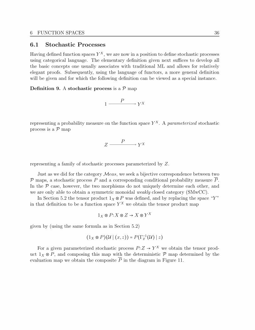
Having defined function spaces Y X , we are now in a position to define stochastic processesusing categorical language. The elementary definition given next suffices to develop allthe basic concepts one usually associates with traditional ML and allows for relativelyelegant proofs. Subsequently, using the language of functors, a more general definitionwill be given and for which the following definition can be viewed as a special instance.
Definition 9. A stochastic process is a P map
1 Y XP
representing a probability measure on the function space Y X . A parameterized stochasticprocess is a P map
Z Y XP
representing a family of stochastic processes parameterized by Z.
Just as we did for the categoryMeas, we seek a bijective correspondence between twoP maps, a stochastic process P and a corresponding conditional probability measure P .In the P case, however, the two morphisms do not uniquely determine each other, andwe are only able to obtain a symmetric monoidal weakly closed category (SMwCC).
In Section 5.2 the tensor product 1X ⊗P was defined, and by replacing the space “Y ”in that definition to be a function space Y X we obtain the tensor product map
1X ⊗ P ∶X ⊗Z →X ⊗ Y X
given by (using the same formula as in Section 5.2)
(1X ⊗ P )(U ∣ (x, z)) = P (Γ−1x (U) ∣ z)
For a given parameterized stochastic process P ∶Z → Y X we obtain the tensor prod-uct 1X ⊗ P , and composing this map with the deterministic P map determined by theevaluation map we obtain the composite P in the diagram in Figure 11.

6 FUNCTION SPACES 37
X ⊗Z
X ⊗ Y X Y
Z
Y X
1X ⊗ P P
δev
P
Figure 11: The defining characteristic property of the evaluation function ev for tensorproducts of conditionals in P.
ThusP (B ∣ (x, z)) = ∫(u,f)∈X⊗Y X (δev)B(u, f)d(1X ⊗ P )(x,z)
= ∫f∈Y X δev(B ∣ Γx(f))dPz= ∫f∈Y X χB(evx(f))dPz= P (ev−1
x (B) ∣ z)and every parameterized stochastic process determines a conditional probability
P ∶X ⊗Z → Y.
Conversely, given a conditional probability P ∶X ⊗Z → Y , we wish to define a param-eterized stochastic process P ∶Z → Y X . We might be tempted to define such a stochasticprocess by letting
P (ev−1x (B) ∣ z) = P (B ∣ (x, z)), (31)
but this does not give a well-defined measure for each z ∈ Z. Recall that a probabilitymeasure cannot be unambiguously defined on an arbitrary generating set for the σ-algebra.We can, however, uniquely define a measure on a π-system14 and then use Dynkin’s π-λtheorem to extend to the entire σ-algebra (e.g., see [10]). This construction requires thefollowing definition.
Definition 10. Given a measurable space (X,ΣX), we can define an equivalence relationon X where x ∼ y if x ∈ A⇔ y ∈ A for all A ∈ ΣX . We call an equivalence class of thisrelation an atom of X. For an arbitrary set A ⊂X, we say that A is
separated if for any two points x, y ∈ A, there is some B ∈ ΣX with x ∈ B and y ∉ B
unseparated if A is contained in some atom of X.
This notion of separation of points is important for finding a generating set on whichwe can define a parameterized stochastic process. The key lemma which we state herewithout proof15 is the following.
14A π-system on X is a nonempty collection of subsets of X that is closed under finite intersections.15This lemma and additional work on symmetric monoidal weakly closed structures on P will appear
in a future paper.

6 FUNCTION SPACES 38
Lemma 11. The class of subsets of Y X
E = ∅ ∪ n
⋂i=1
ev−1xi
(Ai) ∣ xini=1 is separated in X,Ai ∈ ΣY is nonempty and proper
is a π-system which generates the evaluation σ-algebra on Y X .
We can now define many parameterized stochastic processes “adjoint” to P , withthe only requirement being that Equation 31 is satisfied. This is not a deficiency in P,however, but rather shows that we have ample flexibility in this category.
Remark 12. Even when such an expression does provide a well-defined measure as inthe case of finite spaces, it does not yield a unique P . Appendix B provides an elementaryexample illustrating the failure of the bijective correspondence property in this case. Alsoobserve that the proposed defining Equation 31 can be extended to
P (∩ni=1ev−1xi
(Bi) ∣ z) =n
∏i=1
P (Bi ∣ (xi, z))
which does provide a well-defined measure by Lemma 11. However it still does not providea bijective correspondence which is clear as the right hand side implies an independencecondition which a stochastic process need not satisfy. However it does provide for a bi-jective correspondence if we impose an additional independence condition/assumption.Alternatively, by imposing the additional condition that for each z ∈ Z, Pz is a GaussianProcesses we can obtain a bijective correspondence. In Section 6.3 we illustrate in detailhow a joint normal distribution on a finite dimensional space gives rise to a stochasticprocess, and in particular a GP.
Often, we are able to exploit the weak correspondence and use the conditional prob-ability P ∶X → Y rather than the stochastic process P ∶1 → Y X . While carrying lessinformation, the conditional probability is easier to reason with because of our famil-iarity with Bayes’ rule (which uses conditional probabilities) and our unfamiliarity withmeasures on function spaces.
Intuitively it is easier to work with the conditional probability P as we can representthe graph of such functions. In Figure 6.1 the top diagram shows a prior probabilityP ∶1 → R[0,10], which is a stochastic process, depicted by representing its adjunct illus-trating its expected value as well as its 2σ error bars on each coordinate. The bottomdiagram in the same figure illustrates a parameterized stochastic process where the param-eterization is over four measurements. Using the above notation, Z = ∏4
i=1(X × Y )i andP (⋅ ∣ (xi, yi)4
i=1) is a posterior probability measure given four measurements xi, yi4i=1.
These diagrams were generated under the hypothesis that the process is a GP.

6 FUNCTION SPACES 39
Figure 12: The top diagram shows a (prior) stochastic process represented by its adjunctP ∶ [0,10]→ R and characterized by its expected value and covariance. The bottom dia-gram shows a parameterized stochastic process (the same process), also expressed by itsadjunct, where the parameterization is over four measurements.
6 FUNCTION SPACES 40
6.2 Gaussian Processes
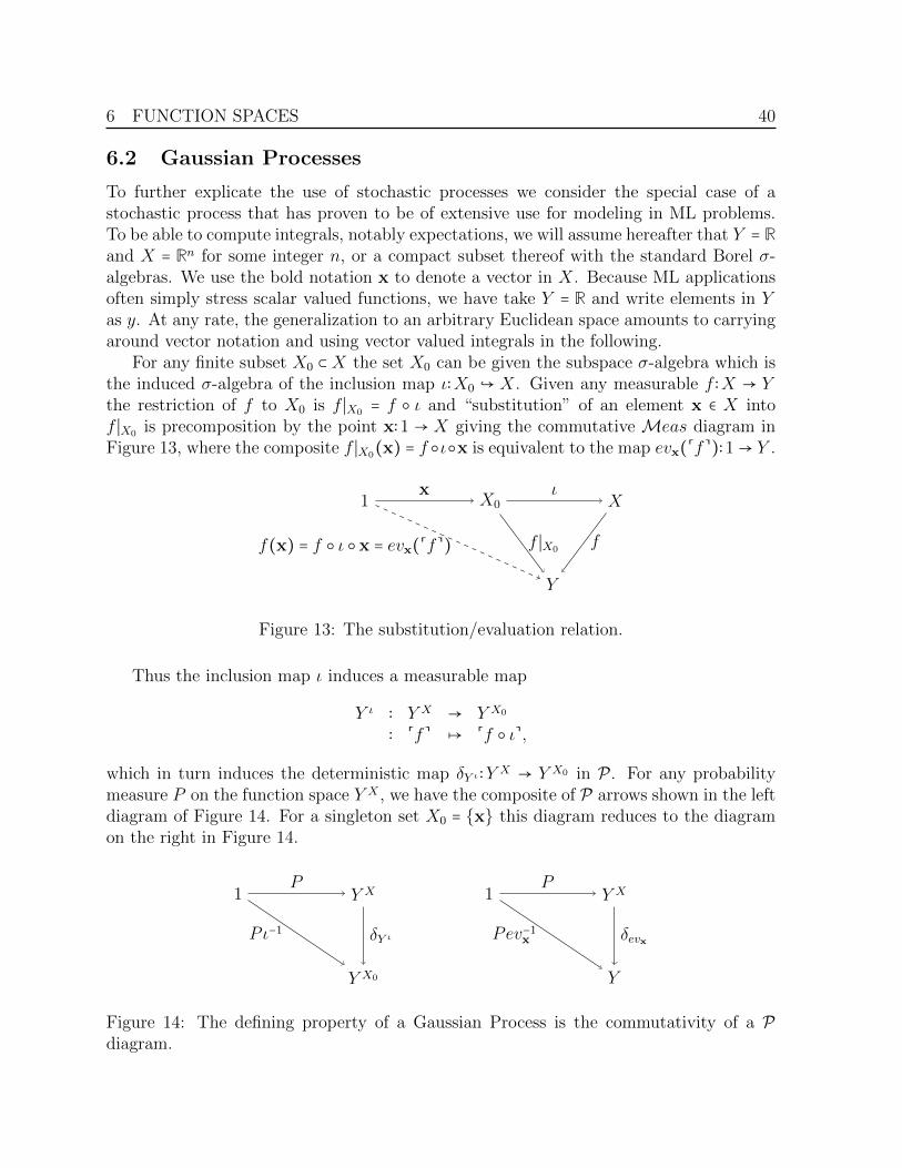
To further explicate the use of stochastic processes we consider the special case of astochastic process that has proven to be of extensive use for modeling in ML problems.To be able to compute integrals, notably expectations, we will assume hereafter that Y = Rand X = Rn for some integer n, or a compact subset thereof with the standard Borel σ-algebras. We use the bold notation x to denote a vector in X. Because ML applicationsoften simply stress scalar valued functions, we have take Y = R and write elements in Yas y. At any rate, the generalization to an arbitrary Euclidean space amounts to carryingaround vector notation and using vector valued integrals in the following.
For any finite subset X0 ⊂X the set X0 can be given the subspace σ-algebra which isthe induced σ-algebra of the inclusion map ι∶X0 X. Given any measurable f ∶X → Ythe restriction of f to X0 is f ∣X0 = f ι and “substitution” of an element x ∈ X intof ∣X0 is precomposition by the point x∶1 → X giving the commutative Meas diagram inFigure 13, where the composite f ∣X0(x) = f ιx is equivalent to the map evx(f)∶1→ Y .
1 X0 X
Y
ιx
ff(x) = f ι x = evx(f) f ∣X0
Figure 13: The substitution/evaluation relation.
Thus the inclusion map ι induces a measurable map
Y ι ∶ Y X → Y X0
∶ f ↦ f ι,
which in turn induces the deterministic map δY ι ∶Y X → Y X0 in P. For any probabilitymeasure P on the function space Y X , we have the composite of P arrows shown in the leftdiagram of Figure 14. For a singleton set X0 = x this diagram reduces to the diagramon the right in Figure 14.
1 Y X
Y X0
P
δY ιPι−1
1 Y X
Y
P
δevxPev−1x
Figure 14: The defining property of a Gaussian Process is the commutativity of a Pdiagram.
6 FUNCTION SPACES 41
Given m ∈ Y X and k a bivariate function k∶X ×X → R, let m∣X0 =m ι ∈ Y X0 denotethe restriction of m to X0 and similiarly let k∣X0 = k (ι× ι) denote the restriction of k toX0 ×X0.
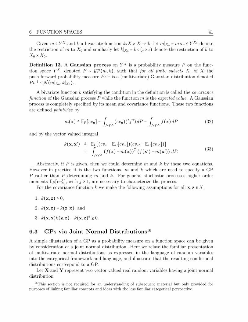
Definition 13. A Gaussian process on Y X is a probability measure P on the func-tion space Y X , denoted P ∼ GP(m,k), such that for all finite subsets X0 of X thepush forward probability measure Pι−1 is a (multivariate) Gaussian distribution denotedPι−1 ∼ N (m∣X0 , k∣X0).
A bivariate function k satisfying the condition in the definition is called the covariancefunction of the Gaussian process P while the function m is the expected value. A Gaussianprocess is completely specified by its mean and covariance functions. These two functionsare defined pointwise by
m(x) ≜ EP [evx] = ∫f∈Y X
(evx)(f)dP = ∫f∈Y X
f(x)dP (32)
and by the vector valued integral
k(x,x′) ≜ EP [(evx − EP [evx])(evx′ − EP [evx′])]= ∫
f∈Y X(f(x) −m(x))T (f(x′) −m(x′)) dP. (33)
Abstractly, if P is given, then we could determine m and k by these two equations.However in practice it is the two functions, m and k which are used to specify a GPP rather than P determining m and k. For general stochastic processes higher ordermoments EP [evjx], with j > 1, are necessary to characterize the process.
For the covariance function k we make the following assumptions for all x,z ∈X,
1. k(x,z) ≥ 0,
2. k(x,z) = k(z,x), and
3. k(x,x)k(z,z) − k(x,z)2 ≥ 0.
6.3 GPs via Joint Normal Distributions16
A simple illustration of a GP as a probability measure on a function space can be givenby consideration of a joint normal distribution. Here we relate the familiar presentationof multivariate normal distributions as expressed in the language of random variablesinto the categorical framework and language, and illustrate that the resulting conditionaldistributions correspond to a GP.
Let X and Y represent two vector valued real random variables having a joint normaldistribution
16This section is not required for an understanding of subsequent material but only provided forpurposes of linking familiar concepts and ideas with the less familiar categorical perspective.
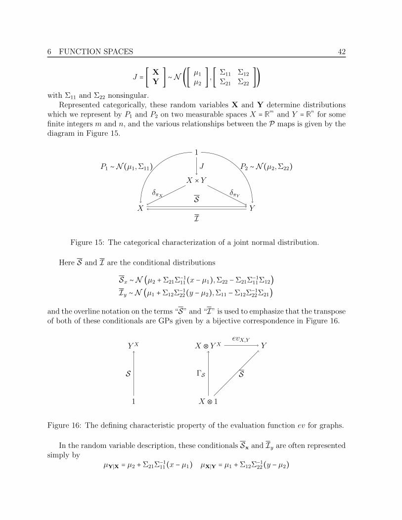
6 FUNCTION SPACES 42
J = [ XY
] ∼ N ([ µ1
µ2] , [ Σ11 Σ12
Σ21 Σ22])
with Σ11 and Σ22 nonsingular.Represented categorically, these random variables X and Y determine distributions
which we represent by P1 and P2 on two measurable spaces X = Rmand Y = Rn
for somefinite integers m and n, and the various relationships between the P maps is given by thediagram in Figure 15.
1
X × Y
X Y
J
δπX δπY
P1 ∼ N (µ1,Σ11) P2 ∼ N (µ2,Σ22)
S
I
Figure 15: The categorical characterization of a joint normal distribution.
Here S and I are the conditional distributions
Sx ∼ N (µ2 +Σ21Σ−111(x − µ1),Σ22 −Σ21Σ−1
11Σ12)Iy ∼ N (µ1 +Σ12Σ−1
22(y − µ2),Σ11 −Σ12Σ−122Σ21)
and the overline notation on the terms “S” and “I” is used to emphasize that the transposeof both of these conditionals are GPs given by a bijective correspondence in Figure 16.
X ⊗ 1
X ⊗ Y X Y
1
Y X
ΓS S
evX,Y
S
Figure 16: The defining characteristic property of the evaluation function ev for graphs.
In the random variable description, these conditionals Sx and Iy are often representedsimply by
µY∣X = µ2 +Σ21Σ−111(x − µ1) µX∣Y = µ1 +Σ12Σ−1
22(y − µ2)

7 BAYESIAN MODELS FOR FUNCTION ESTIMATION 43
andΣY∣X = Σ22 −Σ21Σ−1
11Σ12 ΣX∣Y = Σ11 −Σ12Σ−122
It is easily verified that this pair S,I forms a sampling distribution/inference mappair; i.e., the joint distribution can be expressed in terms of the prior X and samplingdistribution S or in terms of the prior Y and inference map I. It is clear from thisexample that what one calls the sampling distribution and inference map depends uponthe perspective of what is being estimated.
In subsequent developments, we do not assume a joint normal distribution on thespaces X and Y . If such an assumption is reasonable, then the following constructionsare greatly simplified by the structure expressed in Figure 15. As noted previously, it isknowledge of the relationship between the distributions P1 and P2 which characterize thejoint and, is the main modeling problem. Thus the two perspectives on the problem areto find the conditionals, or equivalently, find the prior on Y X which specifies a functionX → Y along with the noise model which is “built into” the sampling distribution.
7 Bayesian Models for Function Estimation
We now have all the necessary tools to build several Bayesian models, both parametricand nonparametric, which illustrate the model building process for ML using CT. To saywe are building Bayesian models means we are constructing the two P arrows, PH andS, corresponding to (1) the prior probability, and (2) the sampling distribution of thediagram in Figure 2. The sampling distribution will generally be a composite of severalsimple P arrows. We start with the nonparametric models which are in a modeling sensemore basic than the parametric models involving a fixed finite number of parameters to bedetermined. The inference maps I for all of the models will be constructed in Section 8.
7.1 Nonparametric Models
In estimation problems where the unknown quantity of interest is a function f ∶ X → Y ,our hypothesis space H will be the function space Y X . However, simply expressing thehypothesis space as Y X appears untenable because, in supervised learning, we nevermeasure Y X directly, but only measure a finite number of sampling points (xi, yi)Ni=1
satisfying some measurement model such as yi = f(xi) + ε where f is an “ideal” functionwe seek to determine.
With precise knowledge of the input state x and assuming a generic stochastic processP ∶1 → Y X , we are led to propose either the left δx⋉P or right δx⋊P tensor productas a prior on the hypothesis space X ⊗ Y X . However, when one of the components ina left or right tensor product is a Dirac measure, then both the left and right tensorscoincide and the choice of right or left tensor is irrelevant. In this case, we denote thecommon probability measure by δx ⊗ P . Moreover, a simple calculation shows the prior

7 BAYESIAN MODELS FOR FUNCTION ESTIMATION 44
δx ⊗ P = ΓP (⋅ ∣ x), the graph of P at x. Thus our proposed model, in analogy to thegeneric Bayesian model, is given by the diagram in Figure 17.17
1
X ⊗ Y X X ⊗ Y
d is measurement dataΓP (⋅ ∣ x) d
S
Figure 17: The generic nonparametric Bayesian model for stochastic processes.
By a nonparametric (Bayesian) model, we mean any model which fits into the schemeof Figure 17. For all of our analysis purposes we take P ∼ GP(m,k). A data measurementd, corresponding to a collection of sample data xi, yi is, in ML applications, generallytaken as a Dirac measure, d = δ(x,y). As in all Bayesian problems, the measurement dataxi, yiNi=1 can be analyzed either sequentially or as a single batch of data. For analysispurpose in Section 8, we consider the data one point at a time (sequentially).
7.1.1 Noise Free Measurement Model
In the noise free measurement model, we make the hypothesis that the data we observe—consisting of input output pairs (xi, yi) ∈ X × Y—satisfies the condition that yi = f(xi)where f is the unknown function we are seeking to estimate. While the actual measureddata will generally not satisfy this hypothesis, this model serves both as an idealizationand a building block for the subsequent noisy measurement model.
Using the fundamental maps Γ⋅∶Y X → (X⊗Y )X and ev∶X⊗(X⊗Y )X →X⊗Y gives asequence of measurable maps which determine corresponding deterministic P maps. Thiscomposite, shown in Figure 18, is our noise free sampling distribution.
X ⊗ Y X X ⊗ (X ⊗ Y )X X ⊗ Y1⊗ δΓ δev
Snf = composite
Figure 18: The noise free sampling distribution Snf .
This deterministic sampling distribution is given by the calculation of the composition,
17It would be interesting to analyze the more general case where there is uncertainty in the input statealso and take the prior as Q⋊P or Q⋉P for some measure Q on X.

7 BAYESIAN MODELS FOR FUNCTION ESTIMATION 45
i.e., evaluating the integral
Snf(U ∣ (x, f)) = ∫(u,g)∈X⊗(X⊗Y )X(δev)U(u, g)d(1⊗ δΓ)(x,f) for U ∈ ΣX⊗Y
= (δev)U(x,Γf)= δΓf (x)(U)= δ(x,f(x))(U)= δ(Γx(evx(f)))(U) because (x, f(x)) = Γx(evx(f))= χU(Γx(evx(f)))= χev−1x (Γ−1
x(U))(f).
Using the commutativity of Figure 10, the noise free sampling distribution can also bewritten as Snf(U ∣ (x, f)) = χΓ−1⋅ (ev−1x (U))(f).
Precomposing the sampling distribution with this prior probability measure the com-posite
(Snf ΓP (⋅ ∣ x))(U) = ∫(u,f)∈X⊗Y X Snf(U ∣ (u, f))d(ΓP (⋅ ∣ x)´¹¹¹¹¹¹¹¹¹¹¹¹¹¸¹¹¹¹¹¹¹¹¹¹¹¹¹¶=PΓ−1
x
) for U ∈ ΣX⊗Y
= ∫f∈Y X Snf(U ∣ Γx(f))dP= ∫f∈Y X χΓ−1⋅ (ev−1x (U))(f)dP= P (Γ−1
⋅ (ev−1x (U)))
(34)
By the relation Γx evx = evx Γ⋅ this can also be written as
(Snf ΓP (⋅ ∣ x))(U) = P (ev−1x (Γ−1
x (U))).
Given that the probability measure P is specified as a Gaussian process (which isdefined in terms of how it restricts to finite subspaces X0 ⊂ X), for computational pur-poses we need to consider the push forward probability measure of P on Y X to Y X0 asin Figure 14. Taking the special case with X0 = x, the pushforward corresponds tocomposition with the deterministic projection map δevx . Starting with the diagram ofFigure 10, precomposing with P and postcomposition with the deterministic map δπY διgives the diagram in Figure 19. Then we can use the fact P projected onto any coordinateis a Gaussian distribution to compute the likelihood that a measurement will occur in ameasurable set B ⊂ Y .
1 Y X (X ⊗ Y )X X ⊗ Y
Y
P ∼ GP(m,k) Γ⋅ evx
δπYδevxPev−1
x ∼ N (m(x), k(x,x))
Figure 19: The distribution P ∼ GP(m,k) can be evaluated on rectangles U = A ×B byprojecting onto the given x coordinate.
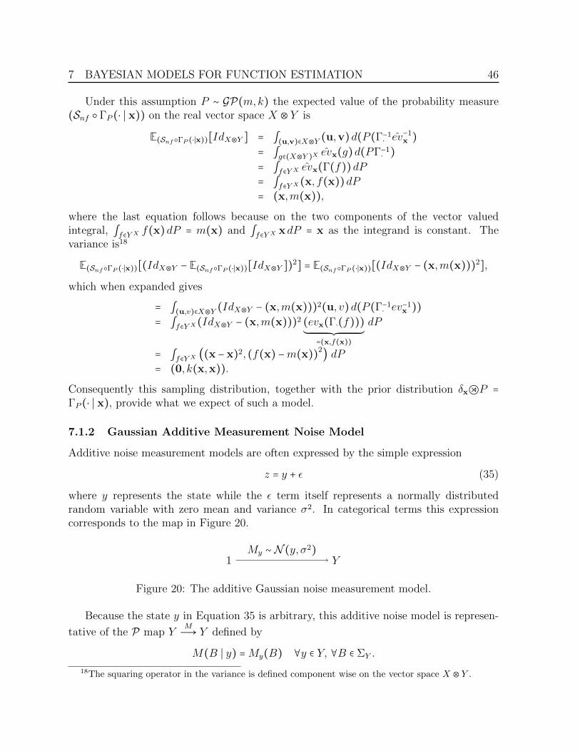
7 BAYESIAN MODELS FOR FUNCTION ESTIMATION 46
Under this assumption P ∼ GP(m,k) the expected value of the probability measure(Snf ΓP (⋅ ∣ x)) on the real vector space X ⊗ Y is
E(SnfΓP (⋅∣x))[IdX⊗Y ] = ∫(u,v)∈X⊗Y (u,v)d(P (Γ−1⋅ ev
−1x )
= ∫g∈(X⊗Y )Xevx(g)d(PΓ−1
⋅ )= ∫f∈Y X evx(Γ(f))dP= ∫f∈Y X(x, f(x))dP= (x,m(x)),
where the last equation follows because on the two components of the vector valuedintegral, ∫f∈Y X f(x)dP = m(x) and ∫f∈Y X xdP = x as the integrand is constant. Thevariance is18
E(SnfΓP (⋅∣x))[(IdX⊗Y − E(SnfΓP (⋅∣x))[IdX⊗Y ])2] = E(SnfΓP (⋅∣x))[(IdX⊗Y − (x,m(x)))2],
which when expanded gives
= ∫(u,v)∈X⊗Y (IdX⊗Y − (x,m(x)))2(u, v)d(P (Γ−1⋅ ev
−1x ))
= ∫f∈Y X(IdX⊗Y − (x,m(x)))2 (evx(Γ⋅(f)))´¹¹¹¹¹¹¹¹¹¹¹¹¹¹¹¹¹¹¹¹¹¹¹¹¹¹¹¹¹¹¸¹¹¹¹¹¹¹¹¹¹¹¹¹¹¹¹¹¹¹¹¹¹¹¹¹¹¹¹¹¹¹
=(x,f(x))
dP
= ∫f∈Y X ((x − x)2, (f(x) −m(x))2) dP= (0, k(x,x)).
Consequently this sampling distribution, together with the prior distribution δx⋊P =ΓP (⋅ ∣ x), provide what we expect of such a model.
7.1.2 Gaussian Additive Measurement Noise Model
Additive noise measurement models are often expressed by the simple expression
z = y + ε (35)
where y represents the state while the ε term itself represents a normally distributedrandom variable with zero mean and variance σ2. In categorical terms this expressioncorresponds to the map in Figure 20.
1 YMy ∼ N (y, σ2)
Figure 20: The additive Gaussian noise measurement model.
Because the state y in Equation 35 is arbitrary, this additive noise model is represen-
tative of the P map YMÐ→ Y defined by
M(B ∣ y) =My(B) ∀y ∈ Y, ∀B ∈ ΣY .
18The squaring operator in the variance is defined component wise on the vector space X ⊗ Y .
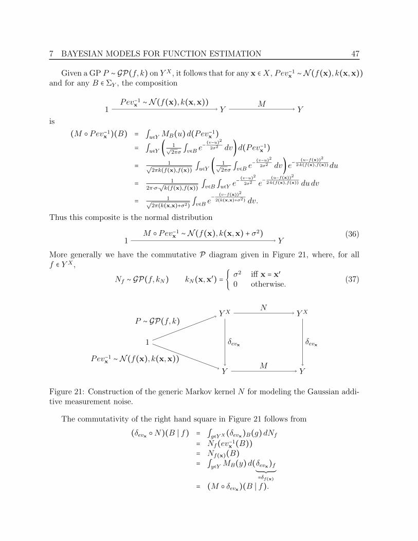
7 BAYESIAN MODELS FOR FUNCTION ESTIMATION 47
Given a GP P ∼ GP(f, k) on Y X , it follows that for any x ∈X, Pev−1x ∼ N (f(x), k(x,x))
and for any B ∈ ΣY , the composition
1 Y YPev−1
x ∼ N (f(x), k(x,x)) M
is
(M Pev−1x )(B) = ∫u∈Y MB(u)d(Pev−1
x )= ∫u∈Y ( 1√
2πσ ∫v∈B e−(v−u)22σ2 dv)d(Pev−1
x )
= 1√2πk(f(x),f(x)) ∫u∈Y ( 1√
2πσ ∫v∈B e−(v−u)22σ2 dv) e−
(u−f(x))22⋅k(f(x),f(x))du
= 1
2π⋅σ⋅√k(f(x),f(x)) ∫v∈B ∫u∈Y e
−(v−u)22σ2 e−
(u−f(x))22⋅k(f(x),f(x)) dudv
= 1√2π(k(x,x)+σ2) ∫v∈B e
−(v−f(x))2
2(k(x,x)+σ2) dv.
Thus this composite is the normal distribution
1 YM Pev−1
x ∼ N (f(x), k(x,x) + σ2) (36)
More generally we have the commutative P diagram given in Figure 21, where, for allf ∈ Y X ,
Nf ∼ GP(f, kN) kN(x,x′) = σ2 iff x = x′
0 otherwise.(37)
1
Y X Y X
Y Y
P ∼ GP(f, k)N
Pev−1x ∼ N (f(x), k(x,x))
M
δevx δevx
Figure 21: Construction of the generic Markov kernel N for modeling the Gaussian addi-tive measurement noise.
The commutativity of the right hand square in Figure 21 follows from
(δevx N)(B ∣ f) = ∫g∈Y X(δevx)B(g)dNf
= Nf(ev−1x (B))
= Nf(x)(B)= ∫y∈Y MB(y)d(δevx)f
²=δf(x)
= (M δevx)(B ∣ f).

7 BAYESIAN MODELS FOR FUNCTION ESTIMATION 48
With this Gaussian additive noise measurement model N our sampling distributionSnf can easily be modified by incorporating the additional map N into the sequence inFigure 18 to yield the Gaussian additive noise sampling distribution model Sn shown inFigure 22.
X ⊗ Y X X ⊗ Y X X ⊗ (X ⊗ Y )X X ⊗ Y1X ⊗N 1X ⊗ δΓ⋅ δev
Sn = composite
Figure 22: The sampling distribution model in P with additive Gaussian noise.
Here 1X ⊗N is, by the definition given in Section 5.2,
(1X ⊗N) (U, (x, f)) = N(Γ−1x (U) ∣ f)
so the nondeterministic noisy sampling distribution is given by
Sn(U ∣ (x, f)) = (Snf (1⊗N)) (U ∣ (x, f)) for U ∈ ΣX⊗Y
= ∫(u,g)∈X⊗Y X(Snf)U(u, g)d(N(Γ−1x (⋅) ∣ f)
= ∫g∈Y X(Snf)U(Γx(g))dN(⋅ ∣ f)= ∫g∈Y X(Snf)(U ∣ (x, g))dN(⋅ ∣ f)= ∫g∈Y X χΓ−1⋅ (ev−1x (U))(g)dN(⋅ ∣ f)= N (Γ−1
⋅ (ev−1x (U)) ∣ f)
= N (ev−1x (Γ−1
x (U)) ∣ f)= Nfev−1
x (Γ−1x (U)).
(38)
Just as we did for the GP P ∶1 → Y X in Figure 19, each GP Nf can be analyzed byits push forward measures onto any coordinate x ∈X to obtain the diagram in Figure 23.
1 Y X (X ⊗ Y )X X ⊗ Y
Y
Nf ∼ GP(f, kN) δΓ⋅ δevx
δπYδevxNf (ev−1
x (⋅)) ∼ N (f(x), σ2)
Figure 23: The GP Nf can be evaluated on rectangles U = A ×B by projecting onto thegiven x coordinate.
Taking U as a rectangle, U = A ×B, with A ∈ ΣX and B ∈ ΣY , the likelihood that a

7 BAYESIAN MODELS FOR FUNCTION ESTIMATION 49
measurement will occur in the rectangle conditioned on (x, f) is given by
Sn(A ×B ∣ (x, f)) = Nfev−1x (Γ−1
x (A ×B))= δx(A) ⋅Nfev−1
x (B)= δx(A) ⋅ 1√
2πσ ∫y∈B e−(y−f(x))2
2σ2 dy.
Using the associativity property of categories, from Figure 22 with a prior ΓP (⋅ ∣ x)on X ⊗ Y X , the composite Sn ΓP (⋅ ∣ x) can be decomposed as
Sn ΓP (⋅ ∣ x) = Snf ((1X ⊗N) ΓP (⋅ ∣ x))
while the term ((1X ⊗N) ΓP (⋅ ∣ x)) = ΓNP (⋅ ∣ x) follows from the commutativity of thediagram in Figure 24, where, as shown in Equation 36, M Pev−1
x ∼ N (m,k(x,x) + σ2)which implies N P ∼ GP(m,k + kN).
1
X
X
Y X
Y X
X ⊗ Y X
X ⊗ Y X
1
X ⊗ Y X
δx
1X
P
N
ΓP (⋅ ∣ x)
1X ⊗N
δπX
δπX
δπY X
δπY X
ΓNP (⋅ ∣ x)
Figure 24: The composite of the prior and noise measurement model is the graph of a GPat x.
Using the fact Sn ΓP (⋅ ∣ x) = Snf ΓNP (⋅ ∣ x), the expected value of the compositeSn ΓP (⋅ ∣ x) is readily shown to be
E(SnΓP (⋅∣x))[IdX⊗Y ] = (x,m(x))while the variance is
E(SnΓP (⋅∣x))[(IdX⊗Y − E(SnΓP (⋅∣x))[IdX⊗Y ])2] = (0, k(x,x) + σ2).
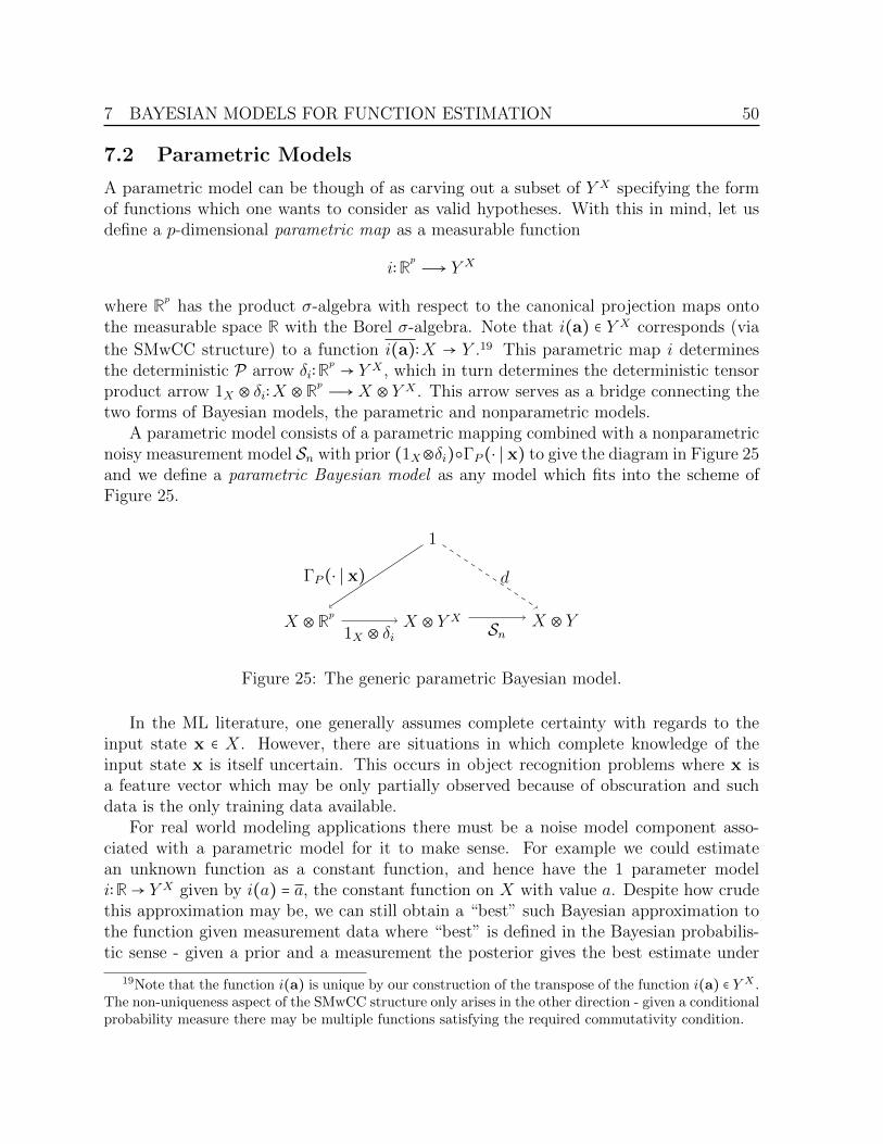
7 BAYESIAN MODELS FOR FUNCTION ESTIMATION 50
7.2 Parametric Models
A parametric model can be though of as carving out a subset of Y X specifying the formof functions which one wants to consider as valid hypotheses. With this in mind, let usdefine a p-dimensional parametric map as a measurable function
i∶Rp Ð→ Y X
where Rphas the product σ-algebra with respect to the canonical projection maps onto
the measurable space R with the Borel σ-algebra. Note that i(a) ∈ Y X corresponds (via
the SMwCC structure) to a function i(a)∶X → Y .19 This parametric map i determinesthe deterministic P arrow δi∶Rp → Y X , which in turn determines the deterministic tensorproduct arrow 1X ⊗ δi∶X ⊗ Rp Ð→X ⊗ Y X . This arrow serves as a bridge connecting thetwo forms of Bayesian models, the parametric and nonparametric models.
A parametric model consists of a parametric mapping combined with a nonparametricnoisy measurement model Sn with prior (1X⊗δi)ΓP (⋅ ∣ x) to give the diagram in Figure 25and we define a parametric Bayesian model as any model which fits into the scheme ofFigure 25.
1
X ⊗ RpX ⊗ Y X X ⊗ Y
ΓP (⋅ ∣ x)
1X ⊗ δi
d
Sn
Figure 25: The generic parametric Bayesian model.
In the ML literature, one generally assumes complete certainty with regards to theinput state x ∈ X. However, there are situations in which complete knowledge of theinput state x is itself uncertain. This occurs in object recognition problems where x isa feature vector which may be only partially observed because of obscuration and suchdata is the only training data available.
For real world modeling applications there must be a noise model component asso-ciated with a parametric model for it to make sense. For example we could estimatean unknown function as a constant function, and hence have the 1 parameter modeli∶R→ Y X given by i(a) = a, the constant function on X with value a. Despite how crudethis approximation may be, we can still obtain a “best” such Bayesian approximation tothe function given measurement data where “best” is defined in the Bayesian probabilis-tic sense - given a prior and a measurement the posterior gives the best estimate under
19Note that the function i(a) is unique by our construction of the transpose of the function i(a) ∈ Y X .The non-uniqueness aspect of the SMwCC structure only arises in the other direction - given a conditionalprobability measure there may be multiple functions satisfying the required commutativity condition.
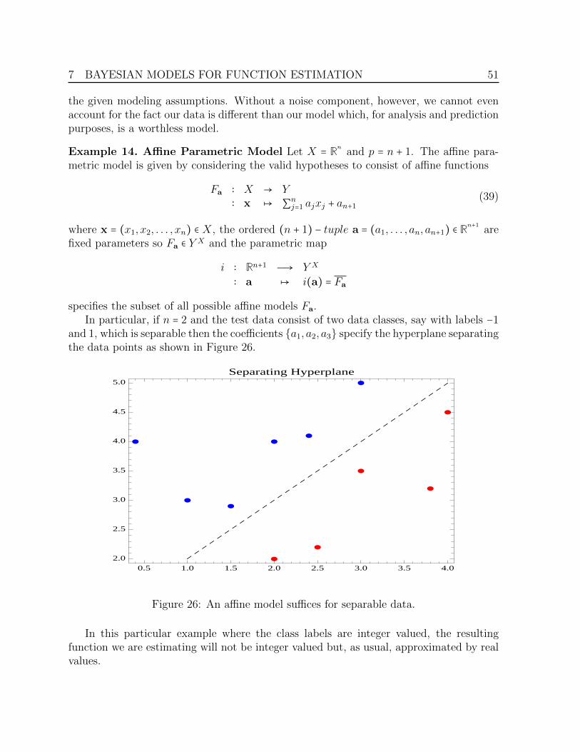
7 BAYESIAN MODELS FOR FUNCTION ESTIMATION 51
the given modeling assumptions. Without a noise component, however, we cannot evenaccount for the fact our data is different than our model which, for analysis and predictionpurposes, is a worthless model.
Example 14. Affine Parametric Model Let X = Rnand p = n + 1. The affine para-
metric model is given by considering the valid hypotheses to consist of affine functions
Fa ∶ X → Y∶ x ↦ ∑n
j=1 ajxj + an+1(39)
where x = (x1, x2, . . . , xn) ∈ X, the ordered (n + 1) − tuple a = (a1, . . . , an, an+1) ∈ Rn+1are
fixed parameters so Fa ∈ Y X and the parametric map
i ∶ Rn+1 Ð→ Y X
∶ a ↦ i(a) = Fa
specifies the subset of all possible affine models Fa.In particular, if n = 2 and the test data consist of two data classes, say with labels −1
and 1, which is separable then the coefficients a1, a2, a3 specify the hyperplane separatingthe data points as shown in Figure 26.
0.5 1.0 1.5 2.0 2.5 3.0 3.5 4.0
2.0
2.5
3.0
3.5
4.0
4.5
5.0Separating Hyperplane
Figure 26: An affine model suffices for separable data.
In this particular example where the class labels are integer valued, the resultingfunction we are estimating will not be integer valued but, as usual, approximated by realvalues.

7 BAYESIAN MODELS FOR FUNCTION ESTIMATION 52
Such parametric models are useful to avoid over fitting data because the number ofparameters are finite and fixed with respect to the number of measurements in contrastto nonparametric methods in which each measurement serves as a parameter defining theupdated probability measure on Y X .
More generally, for any parametric map i take the canonical basis vectors ej, whichare the jth unit vector in Rp
, and let the image of the basis elements ejpj=1 under theparametric map i be i(ej) = fj ∈ Y X . Because Y X forms a real vector space underpointwise addition and scalar multiplication, (f + g)(x) = f(x) + g(x) and (αf)(x) =α(f(x)) for all f, g ∈ Y X ,x ∈ X, and α ∈ R, we observe that the “image carved out” bythe parametric map i is just the span of the image of the basis elements ejpj=1. In theabove example fj = πj, for j = 1,2 where πj is the canonical projection map R2 → R, andf3 = 1, the constant function with value 1 on all points x ∈ X. Thus the image is asspecified by the Equation 39.
Example 15. Elliptic Parametric Model When the data is not linearly separable asin the previous example, but rather of the form shown in Figure 27, then a higher orderparametric model is required.
-1 0 1 2 3 4
2.0
2.5
3.0
3.5
4.0
4.5
5.0
Separating Ellipse
Figure 27: An elliptic parametric model suffices to separate the data.
Taking X = Rn and p = n2 +n+1, the elliptic parametric model is given by consideringthe valid hypotheses to consist of all elliptic functions
Fa ∶ X → Y∶ x ↦ ∑n
j=1 ajxj +∑nj=1∑n
k=1 an+n(j−1)+kxjxk + an2+n+1(40)
where x = (x1, x2, . . . , xn) ∈X, the ordered (n2+n+1)−tuple a = (a1, . . . , an2+n+1) ∈ Rn2+n+1
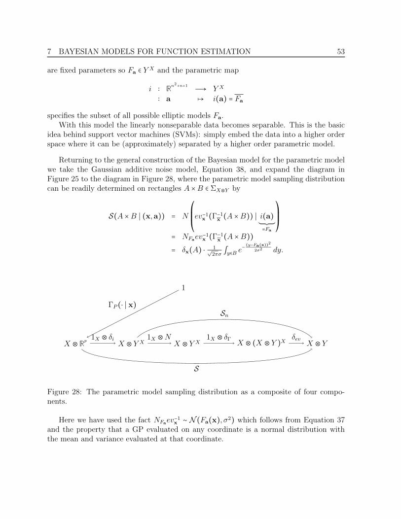
7 BAYESIAN MODELS FOR FUNCTION ESTIMATION 53
are fixed parameters so Fa ∈ Y X and the parametric map
i ∶ Rn2+n+1 Ð→ Y X
∶ a ↦ i(a) = Fa
specifies the subset of all possible elliptic models Fa.With this model the linearly nonseparable data becomes separable. This is the basic
idea behind support vector machines (SVMs): simply embed the data into a higher orderspace where it can be (approximately) separated by a higher order parametric model.
Returning to the general construction of the Bayesian model for the parametric modelwe take the Gaussian additive noise model, Equation 38, and expand the diagram inFigure 25 to the diagram in Figure 28, where the parametric model sampling distributioncan be readily determined on rectangles A ×B ∈ ΣX⊗Y by
S(A ×B ∣ (x,a)) = N
⎛⎜⎜⎝ev−1
x (Γ−1x (A ×B)) ∣ i(a)
±=Fa
⎞⎟⎟⎠
= NFaev−1x (Γ−1
x (A ×B))= δx(A) ⋅ 1√
2πσ ∫y∈B e−(y−Fa(x))2
2σ2 dy.
1
X ⊗ RpX ⊗ Y X X ⊗ Y X X ⊗ (X ⊗ Y )X X ⊗ Y
ΓP (⋅ ∣ x)
1X ⊗ δi 1X ⊗N 1X ⊗ δΓ δev
S
Sn
Figure 28: The parametric model sampling distribution as a composite of four compo-nents.
Here we have used the fact NFaev−1x ∼ N (Fa(x), σ2) which follows from Equation 37
and the property that a GP evaluated on any coordinate is a normal distribution withthe mean and variance evaluated at that coordinate.

8 CONSTRUCTING INFERENCE MAPS 54
8 Constructing Inference Maps
We now proceed to construct the inference maps I for each of the models specified in theprevious section. This construction permits the updating of the GP prior distributions Pfor the nonparametric models and the normal priors P on Rk for the parametric modelsthrough the relation that the posterior measure is given by I d, where d is a datameasurement. The resulting analysis produces the familiar updating rules for the meanand covariance functions characterizing a GP.
8.1 The noise free inference map
Under a prior probability of the form δx ⊗P = ΓP (⋅ ∣ x) on the hypothesis space X ⊗ Y X ,which is a one point measure with respect to the component X, the sampling distributionSnf in Figure 18 can be viewed as a family of deterministic P maps—one for each pointx ∈X.
Y X YSx = δevx
Figure 29: The noise free sampling distributions Sx given the prior δx ⊗P with the diracmeasure on the X component.
Using the property that δevx(B ∣ f) = 1ev−1x (B)(f) for all B ∈ ΣY and f ∈ Y X , the resultingdeterministic sampling distributions (one for each x ∈X) are given by
Sx(B ∣ f) = 1ev−1x (B)(f). (41)
This special case of the prior δx⊗P , which is the most important one for many ML applica-tions and the one implicitly assumed in ML textbooks, permits a complete mathematicalanalysis.
Given the probability measure P ∼ GP(m,k) and Sx = δevx , it follows the compositeis the pushforward probability measure
Sx P = Pev−1x , (42)
which is the special case of Figure 14 with X0 = x. Using the fact that P projectedonto any coordinate is a normal distribution as shown in Figure 30, it follows that theexpected mean is
EPev−1x (IdY ) = EP (evx)= m(x)
while the expected variance is
EPev−1x (IdY − EPev−1x (IdY ))2) = EP (evx − EP (evx))2)= k(x,x).
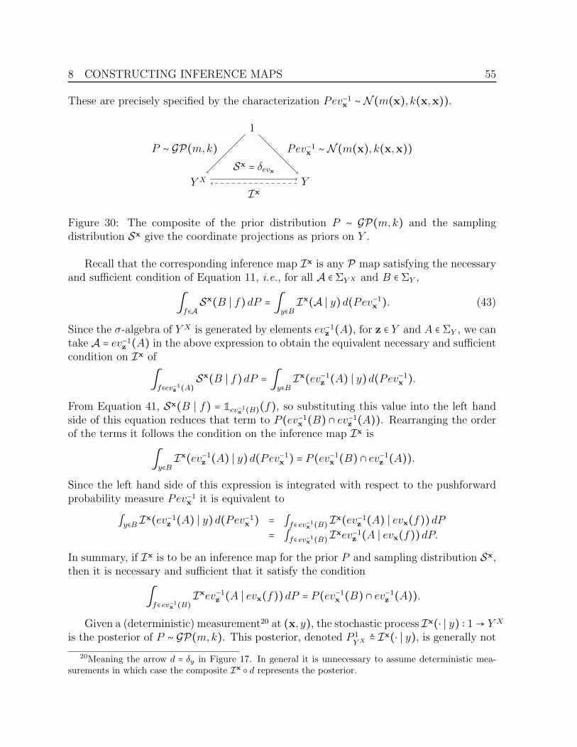
8 CONSTRUCTING INFERENCE MAPS 55
These are precisely specified by the characterization Pev−1x ∼ N (m(x), k(x,x)).
1
Y X Y
P ∼ GP(m,k)Sx = δevx
Ix
Pev−1x ∼ N (m(x), k(x,x))
Figure 30: The composite of the prior distribution P ∼ GP(m,k) and the samplingdistribution Sx give the coordinate projections as priors on Y .
Recall that the corresponding inference map Ix is any P map satisfying the necessaryand sufficient condition of Equation 11, i.e., for all A ∈ ΣY X and B ∈ ΣY ,
∫f∈ASx(B ∣ f)dP = ∫
y∈BIx(A ∣ y)d(Pev−1
x ). (43)
Since the σ-algebra of Y X is generated by elements ev−1z (A), for z ∈ Y and A ∈ ΣY , we can
take A = ev−1z (A) in the above expression to obtain the equivalent necessary and sufficient
condition on Ix of
∫f∈ev−1z (A)
Sx(B ∣ f)dP = ∫y∈BIx(ev−1
z (A) ∣ y)d(Pev−1x ).
From Equation 41, Sx(B ∣ f) = 1ev−1x (B)(f), so substituting this value into the left handside of this equation reduces that term to P (ev−1
x (B) ∩ ev−1z (A)). Rearranging the order
of the terms it follows the condition on the inference map Ix is
∫y∈BIx(ev−1
z (A) ∣ y)d(Pev−1x ) = P (ev−1
x (B) ∩ ev−1z (A)).
Since the left hand side of this expression is integrated with respect to the pushforwardprobability measure Pev−1
x it is equivalent to
∫y∈B Ix(ev−1z (A) ∣ y)d(Pev−1
x ) = ∫f∈ ev−1x (B)Ix(ev−1
z (A) ∣ evx(f))dP= ∫f∈ ev−1x (B)
Ixev−1z (A ∣ evx(f))dP.
In summary, if Ix is to be an inference map for the prior P and sampling distribution Sx,then it is necessary and sufficient that it satisfy the condition
∫f∈ ev−1x (B)
Ixev−1z (A ∣ evx(f))dP = P (ev−1
x (B) ∩ ev−1z (A)).
Given a (deterministic) measurement20 at (x, y), the stochastic process Ix(⋅ ∣ y) ∶ 1→ Y X
is the posterior of P ∼ GP(m,k). This posterior, denoted P 1Y X
≜ Ix(⋅ ∣ y), is generally not
20Meaning the arrow d = δy in Figure 17. In general it is unnecessary to assume deterministic mea-surements in which case the composite Ix d represents the posterior.

8 CONSTRUCTING INFERENCE MAPS 56
unique. However we can require that the posterior P 1Y X
be a GP specified by updatedmean and covariance functions m1 and k1 respectively, which depend upon the condition-ing value y, so P 1
Y X∼ GP(m1, k1). To determine P 1
Y X, and hence the desired inference
map Ix, we make a hypothesis about the updated mean and covariance functions m1 andk1 characterizing P 1
Y Xgiven a measurement at the pair (x, y) ∈X ×Y . Let us assume the
updated mean function is of the form
m1(z) =m(z) + k(z,x)k(x,x)(y −m(x)) (44)
and the updated covariance function is of the form
k1(w,z) = k(w,z) − k(w,x)k(x,z)k(x,x) . (45)
To prove these updated functions suffice to specify the inference map Ix(⋅ ∣ y) = P 1Y X
∼GP(m1, k1) satisfying the necessary and sufficient condition we simply evaluate
∫f∈ ev−1x (B)
Ixev−1z (A ∣ evx(f))dP
by substituting Ix(⋅ ∣ f(x)) = P 1(m1, k1) and verify that it yields P (ev−1x (B) ∩ ev−1
z (A)).Since Ixev−1
z (⋅ ∣ f(x)) = P 1Y Xev−1
x is a normal distribution of mean
m1(z) =m(x) + k(z,x)k(x,x) ⋅ (f(x) −m(x))
and covariance
k1(z,z) = k(z,z) − k(z,x)2
k(x,x)it follows that
∫f∈ ev−1x (B)
Ixev−1z (A ∣ evx(f))dP = ∫
f∈ ev−1x (B)
⎛⎝
1√2πk1(z,z) ∫v∈A
e−(m1(z)−v)2
2k1(z,z) dv⎞⎠dP
which can be expanded to
∫f∈ ev−1x (B)
⎛⎝
1√2πk1(z,z) ∫v∈A
e−(m(z)+ k(z,x)
k(x,x) (f(x)−m(x))−v)2
2k1(z,z) dv⎞⎠dP
and equals
∫y∈B
⎛⎝
1√2πk1(z,z) ∫v∈A
e−(m(z)+ k(z,x)
k(x,x) (y−m(x))−v)2
2k1(z,z) dv⎞⎠dPev−1
x .

8 CONSTRUCTING INFERENCE MAPS 57
Using PY Xev−1x ∼ N (m(x), k(x,x)) we can rewrite the expression as
1√2π ∣ Ω ∣ ∫y∈B ∫v∈A
e−12(u−u)TΩ−1(u−u)dv dy
where
u = ( yv
) u = ( m(x)m(z) )
and
Ω = ( k[x,x] k[x,z]k[z,x] k[z,z] ) ,
which we recognize as a normal distribution N (u,Ω).On the other hand, we claim that
1 Yx × Yz,P (ev−1
x (⋅) ∩ ev−1z (⋅))
where Yx and Yz are two copies of Y , is also a normal distribution of mean u = (m(x),m(z))with covariance matrix Ω.21 To prove our claim consider the P diagram in Figure 31 whereX0 = x,z, ι ∶ X0 X is the inclusion map referenced in Section 6.2, and evx × evz isan isomorphism between the two different representations of the set of all measurablefunctions Y X0 alluded to in the second paragraph of Section 6.
1 Y X
Yx
Yz
Y X0 Yx × YzP δY ι
δevx
δevz
δπYx
δπYz
δevx
δevz
δevx×evz
N (m(x), k(x,x))
N (m(z), k(z,z))
Figure 31: Proving the joint distribution δevx×evz δY ι P = P (ev−1x (⋅) ∩ ev−1
z (⋅))) is anormal distribution N (u,Ω).
21Formally the arguments should be numbered in the given probability measure as P (ev−1x (#1) ∩ev−1z (#2)) because ev−1x (A) ∩ ev−1z (B) ≠ ev−1x (B) ∩ ev−1z (A). However the subscripts can be used toidentify which component measurable sets are associated with each argument.
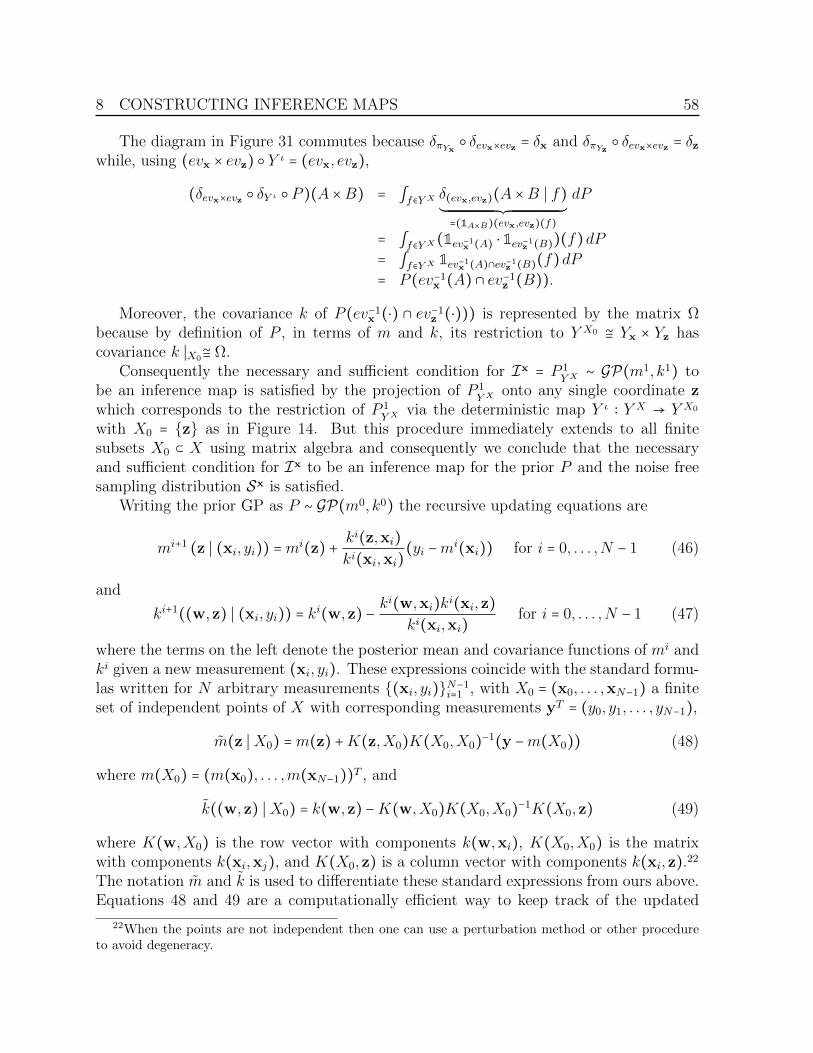
8 CONSTRUCTING INFERENCE MAPS 58
The diagram in Figure 31 commutes because δπYx δevx×evz = δx and δπYz δevx×evz = δzwhile, using (evx × evz) Y ι = (evx, evz),
(δevx×evz δY ι P )(A ×B) = ∫f∈Y X δ(evx,evz)(A ×B ∣ f)´¹¹¹¹¹¹¹¹¹¹¹¹¹¹¹¹¹¹¹¹¹¹¹¹¹¹¹¹¹¹¹¹¹¹¹¹¹¹¹¹¹¹¹¹¹¹¹¹¹¹¹¹¹¹¸¹¹¹¹¹¹¹¹¹¹¹¹¹¹¹¹¹¹¹¹¹¹¹¹¹¹¹¹¹¹¹¹¹¹¹¹¹¹¹¹¹¹¹¹¹¹¹¹¹¹¹¹¹¹¹¶=(1A×B)(evx,evz)(f)
dP
= ∫f∈Y X(1ev−1x (A) ⋅ 1ev−1z (B))(f)dP= ∫f∈Y X 1ev−1x (A)∩ev−1z (B)(f)dP= P (ev−1
x (A) ∩ ev−1z (B)).
Moreover, the covariance k of P (ev−1x (⋅) ∩ ev−1
z (⋅))) is represented by the matrix Ωbecause by definition of P , in terms of m and k, its restriction to Y X0 ≅ Yx × Yz hascovariance k ∣X0≅ Ω.
Consequently the necessary and sufficient condition for Ix = P 1Y X
∼ GP(m1, k1) tobe an inference map is satisfied by the projection of P 1
Y Xonto any single coordinate z
which corresponds to the restriction of P 1Y X
via the deterministic map Y ι ∶ Y X → Y X0
with X0 = z as in Figure 14. But this procedure immediately extends to all finitesubsets X0 ⊂ X using matrix algebra and consequently we conclude that the necessaryand sufficient condition for Ix to be an inference map for the prior P and the noise freesampling distribution Sx is satisfied.
Writing the prior GP as P ∼ GP(m0, k0) the recursive updating equations are
mi+1 (z ∣ (xi, yi)) =mi(z) + ki(z,xi)ki(xi,xi)
(yi −mi(xi)) for i = 0, . . . ,N − 1 (46)
and
ki+1((w,z) ∣ (xi, yi)) = ki(w,z) −ki(w,xi)ki(xi,z)
ki(xi,xi)for i = 0, . . . ,N − 1 (47)
where the terms on the left denote the posterior mean and covariance functions of mi andki given a new measurement (xi, yi). These expressions coincide with the standard formu-las written for N arbitrary measurements (xi, yi)N−1
i=1 , with X0 = (x0, . . . ,xN−1) a finiteset of independent points of X with corresponding measurements yT = (y0, y1, . . . , yN−1),
m(z ∣X0) =m(z) +K(z,X0)K(X0,X0)−1(y −m(X0)) (48)
where m(X0) = (m(x0), . . . ,m(xN−1))T , and
k((w,z) ∣X0) = k(w,z) −K(w,X0)K(X0,X0)−1K(X0,z) (49)
where K(w,X0) is the row vector with components k(w,xi), K(X0,X0) is the matrixwith components k(xi,xj), and K(X0,z) is a column vector with components k(xi,z).22
The notation m and k is used to differentiate these standard expressions from ours above.Equations 48 and 49 are a computationally efficient way to keep track of the updated
22When the points are not independent then one can use a perturbation method or other procedureto avoid degeneracy.
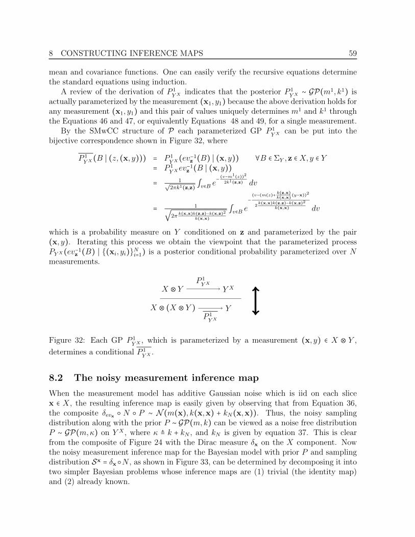
8 CONSTRUCTING INFERENCE MAPS 59
mean and covariance functions. One can easily verify the recursive equations determinethe standard equations using induction.
A review of the derivation of P 1Y X
indicates that the posterior P 1Y X
∼ GP(m1, k1) isactually parameterized by the measurement (x1, y1) because the above derivation holds forany measurement (x1, y1) and this pair of values uniquely determines m1 and k1 throughthe Equations 46 and 47, or equivalently Equations 48 and 49, for a single measurement.
By the SMwCC structure of P each parameterized GP P 1Y X
can be put into thebijective correspondence shown in Figure 32, where
P 1Y X
(B ∣ (z, (x, y))) = P 1Y X
(ev−1z (B) ∣ (x, y)) ∀B ∈ ΣY ,z ∈X,y ∈ Y
= P 1Y Xev−1
z (B ∣ (x, y))
= 1√2πk1(z,z) ∫v∈B e
−(v−m1(z))22k1(z,z) dv
= 1√
2πk(x,x)k(z,z)−k(x,z)2
k(x,x)∫v∈B e
−(v−(m(z)+ k(z,x)
k(x,x) (y−x))2
2k(x,x)k(z,z)−k(x,z)2
k(x,x) dv
which is a probability measure on Y conditioned on z and parameterized by the pair(x, y). Iterating this process we obtain the viewpoint that the parameterized processPY X(ev−1
z (B) ∣ (xi, yi)Ni=1) is a posterior conditional probability parameterized over Nmeasurements.
X ⊗ Y Y X
X ⊗ (X ⊗ Y ) Y
P 1Y X
P 1Y X
Figure 32: Each GP P 1Y X
, which is parameterized by a measurement (x, y) ∈ X ⊗ Y ,
determines a conditional P 1Y X
.
8.2 The noisy measurement inference map
When the measurement model has additive Gaussian noise which is iid on each slicex ∈ X, the resulting inference map is easily given by observing that from Equation 36,the composite δevx N P ∼ N (m(x), k(x,x) + kN(x,x)). Thus, the noisy samplingdistribution along with the prior P ∼ GP(m,k) can be viewed as a noise free distributionP ∼ GP(m,κ) on Y X , where κ ≜ k + kN , and kN is given by equation 37. This is clearfrom the composite of Figure 24 with the Dirac measure δx on the X component. Nowthe noisy measurement inference map for the Bayesian model with prior P and samplingdistribution Sx = δx N , as shown in Figure 33, can be determined by decomposing it intotwo simpler Bayesian problems whose inference maps are (1) trivial (the identity map)and (2) already known.

8 CONSTRUCTING INFERENCE MAPS 60
1
Y X Y X Y
P ∼ N (m,k)
N
N Pδx N P ∼ N (m(x), k(x,x) + kN(x,x)
´¹¹¹¹¹¹¹¹¹¹¹¹¹¹¹¹¹¹¹¹¹¹¹¹¹¹¹¹¹¹¹¹¹¹¹¹¹¹¹¹¹¹¹¹¹¹¹¹¹¹¹¸¹¹¹¹¹¹¹¹¹¹¹¹¹¹¹¹¹¹¹¹¹¹¹¹¹¹¹¹¹¹¹¹¹¹¹¹¹¹¹¹¹¹¹¹¹¹¹¹¹¹¹¶=κ(x,x)
)
δevx
Sx
⇓ Decomposition
1
Y X Y X
P ∼ N (m,k)
N
N P
I∗
1
Y X Y
N P
δx
δx N P
Inf
Figure 33: Splitting the Gaussian additive noise Bayesian model (top diagram) into twoseparate Bayesian models (bottom two diagrams) and composing the inference maps forthese two simple Bayesian models gives the inference map for the original Gaussian addi-tive Bayesian model.
Observe that the composition of the two bottom diagrams is the top diagram. Thebottom diagram on the right is a noise free Bayesian model with GP prior N P andsampling distribution δx whose inference map Inf we have already determined analyticallyin Section 8.1. Given a measurement y ∈ Y at x ∈ X, the inference map is given by theupdating Equations 44 and 45 for the mean and covariance functions characterizing the GPon Y X . The resulting posterior GP on Y X can then be viewed as a measurement on Y X forthe bottom left diagram, which is a Bayesian model with prior P and sampling distributionN . The inference map I⋆ for this diagram is the identity map on Y X , I⋆ = δId
Y X. This is
easy to verify using Bayes product rule (Equation 13), ∫a∈AN(B ∣ a)dP = ∫f∈B δIdY X (A ∣f)d(N P ), for any A,B ∈ ΣY X . Composition of these two inference maps, Inf and I⋆then yields the resulting inference map for the Gaussian additive noise Bayesian model.
With this observation both of the recursive updating schemes given by Equations 46and 47 are valid for the Gaussian additive noise model with k replaced by κ. The corre-sponding standard expressions for the noisy model are then
m(z ∣X0) =m(z) +K(z,X0)K(X0,X0)−1(y −m(X0))
andκ((w,z) ∣X0) = κ(w,z) −K(w,X0)K(X0,X0)−1K(X0,z),
where the quantities like K(w,X0) are as defined previously (following Equation 49)except now k is replaced by κ. For w ≠ z and neither among the measurements X0 these
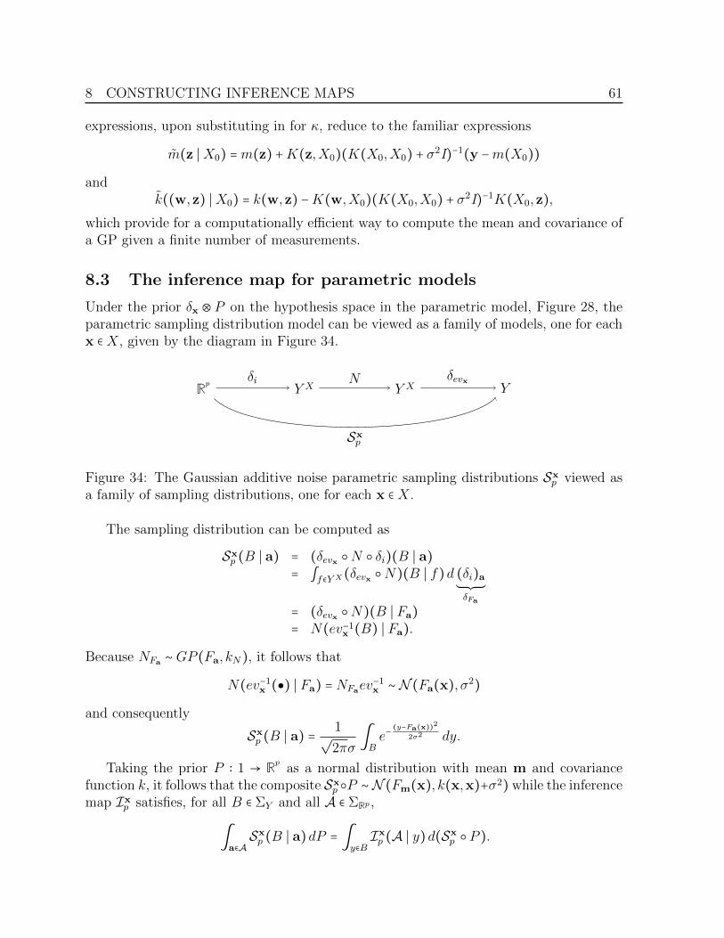
8 CONSTRUCTING INFERENCE MAPS 61
expressions, upon substituting in for κ, reduce to the familiar expressions
m(z ∣X0) =m(z) +K(z,X0)(K(X0,X0) + σ2I)−1(y −m(X0))
andk((w,z) ∣X0) = k(w,z) −K(w,X0)(K(X0,X0) + σ2I)−1K(X0,z),
which provide for a computationally efficient way to compute the mean and covariance ofa GP given a finite number of measurements.
8.3 The inference map for parametric models
Under the prior δx ⊗ P on the hypothesis space in the parametric model, Figure 28, theparametric sampling distribution model can be viewed as a family of models, one for eachx ∈X, given by the diagram in Figure 34.
RpY X Y X Y
δi N δevx
Sxp
Figure 34: The Gaussian additive noise parametric sampling distributions Sxp viewed asa family of sampling distributions, one for each x ∈X.
The sampling distribution can be computed as
Sxp (B ∣ a) = (δevx N δi)(B ∣ a)= ∫f∈Y X(δevx N)(B ∣ f)d (δi)a
±δFa
= (δevx N)(B ∣ Fa)= N(ev−1
x (B) ∣ Fa).
Because NFa ∼ GP (Fa, kN), it follows that
N(ev−1x () ∣ Fa) = NFaev
−1x ∼ N (Fa(x), σ2)
and consequently
Sxp (B ∣ a) = 1√2πσ
∫Be−(y−Fa(x))2
2σ2 dy.
Taking the prior P ∶ 1 → Rpas a normal distribution with mean m and covariance
function k, it follows that the composite Sxp P ∼ N (Fm(x), k(x,x)+σ2) while the inferencemap Ixp satisfies, for all B ∈ ΣY and all A ∈ ΣRp ,
∫a∈ASxp (B ∣ a)dP = ∫
y∈BIxp (A ∣ y)d(Sxp P ).

8 CONSTRUCTING INFERENCE MAPS 62
To determine this inference map Ixp it is necessary to require the parametric map
i ∶ Rp Ð→ Y X
∶ a ↦ ia
be an injective linear homomorphism. Under this condition, which can often be achievedsimply by eliminating redundant modeling parameters, we can explicitly determine theinference map for the parameterized model, denoted Ixp , by decomposing it into twoinference maps as displayed in the diagram in Figure 35.
1
RnY X Y Sxp = Sxn δi
Pi−1P
δi
I⋆
SxnIxn
Sxn Pi−1
Ixp
Figure 35: The inference map for the parametric model is a composite of two inferencemaps.
We first show the stochastic process Pi−1 is a GP and by taking the sampling distri-bution Sxn = δevx N as the noisy measurement model we can use the result of the previoussection to provide us with the inference map Ixn in Figure 35.
Lemma 16. Let k be the matrix representation of the covariance function k. The thepush forward of P N (m, k) by i is a GP Pi−1 ∼ GP(im, k), where k(u,v) = uTkv.
Proof. We need to show that the push forward of Pi−1 by the restriction map Y ι ∶ Y X Ð→ Y X0
is a normal distribution for any finite subspace ι ∶X0 X. Consider the commutate dia-gram in Figure 36, where Yx is a copy of Y , X0 = (x1, . . . ,xn′), and
evx1 × . . . × evxn′ ∶ Y X0 → ∏x∈X0
Yx
is the canonical isomorphism.

8 CONSTRUCTING INFERENCE MAPS 63
1
RnY X
Y X0 ∏x∈X0Yx
Pi−1P
δi
δY ιδY ιi δevx1×...×evxn′
Figure 36: The restriction of Pi−1.
The composite of the measurable maps
((evx1 × . . . × evxn′) Y ι i) (a) = (ia(x1), . . . , ia(xn′)) (50)
from which it follows that the composite map δevx1×...×evxn′ δY ι Pi−1 ∼ N (XT
0 m,XT0 kX0).
Now the diagram
1
RnY X
Pi−1P
δi
I⋆
with the sampling distribution for this Bayesian problem as δi. Let eTj = (0, . . . ,0,1,0, . . . ,0)be the jth unit vector of Rp
and let iej = fj ∈ Y X . The elements fjpj=1 form the compo-nents of a basis for the image of i by the assumed injective property of i. Let this finitebasis have a dual basis f∗j
pj=1 so that f∗k (fj) = δk(j).
Consider the measurable map
f∗1 × . . . × f∗p ∶ Y X → Rp
; g ↦ (f∗1 (g), . . . , f∗p (g)),
Using the linearity of the parameter space Rpit follows a = ∑p
i=1 aiei and consequently
((f∗1 × . . . × f∗p ) i) (a) = (f∗1 (ia), . . . , f∗p (ia))= a using f∗j (ia) = f∗j (∑
pk=1 akfk) = aj

8 CONSTRUCTING INFERENCE MAPS 64
and hence (f∗1 × . . . × f∗p ) i = idRp in Meas. Now it follows the corresponding inferencemap I⋆ = δf∗1 ×...×f∗p because the necessary and sufficient condition for I⋆ is given, for allev−1
z (B) ∈ ΣY X (which generate ΣY X ) and all A ∈ ΣRn , by
∫a∈A
δi(ev−1z (B) ∣ a)dP = ∫
g∈ev−1z (B)I⋆(A ∣ g)dP i−1 (51)
with the left hand term reducing to the expression
∫a∈A
1i−1(ev−1z (B))(a)dP = P (i−1(ev−1z (B)) ∩A).
On the other hand, using I⋆ = δf∗1 ×...×f∗p , the right hand term of Equation 51 also reducesto the same expression since
∫g∈ev−1z (B)δf∗1 ×...×f∗p (A ∣ g)d(Pi−1) = ∫a∈i−1(ev−1z (B))
1((f∗1 ×...×f∗p )i)−1(A)(a)dP= ∫a∈i−1(ev−1z (B))
1A(a)dP= P (i−1(ev−1
z (B)) ∩A)
thus proving I⋆ = δf∗1 ×...×f∗p .Taking
Ixp = I⋆ Ixn ,it follows that for a given measurement (x, y) that the composite is
Ixp = Ixn((f∗1 × . . . × f∗p )−1(⋅) ∣ y) (52)
which is the push forward measure of the GP Ixn(⋅ ∣ y) ∼ GP(i1m, κ1) where (as definedpreviously) κ = k + kN and
i1m(z) = im(z) + κ(z,x)κ(x,x)(y − im(x)) (53)
and
κ1(u,v) = κ(u,v) − κ(u,x)κ(x,v)κ(x,x) . (54)
This GP projected onto any finite subspace ι ∶ X0 X is a normal distribution and, forX0 = x1,x2, . . . ,xn, it follows that
1 Y X Y X0
∏ni=1 Yi ≅ Rn
δY ι
δevx1×...×evxn ∣Y X0δevx1×...×evxn
Ixn( ∣ y) ∼ GP(i1m, κ1)
Ip( ∣ y) ∼ N ((i1m(x1), . . . , i1m(xn))T , κ1 ∣X0)
9 STOCHASTIC PROCESSES AS POINTS 65
where Yi is a copy of Y = R and the restriction δevx1×...×evxn ∣Y X0 is an isomorphism. Theinference map Ip( ∣ y) is the updated normal distribution on Rn
given the measurement(x, y) which can be rewritten as
Ip( ∣ y) ∼ N (m +K(X0,x)κ(x,x)−1(y −mTx), κ1 ∣X0),
where X0 is now viewed as the ordered set X0 = (x1, . . . ,xn) and K(X0,x) is the n-vectorwith components κ(xj,x).
Iterating this updating procedure for N measurements (xi, yi)Ni=1 the N th posteriorcoincides with the analogous noisy measurment inference updating Equations 48 and 49with κ in place of k.
9 Stochastic Processes as Points
Having defined stochastic processes we would be remiss not to mention the Markovprocess—one of the most familiar type of processes used for modeling. Many applica-tions can be approximated by Markov models and a familiar example is the Kalman filterwhich we describe below as it is the archetype. While Kalman filtering is not commonlyviewed as a ML problem, it is useful to put it into perspective with respect to the Bayesianmodeling paradigm.
By looking at Markov processes we are immediately led to a generalization of thedefinition of a stochastic process which is due to Lawvere and Meng [18]. To motivatethis we start with the elementary idea first before giving the generalized definition of astochastic process.
9.1 Markov processes via Functor Categories
Here we assume knowledge of the definition of a functor, and refer the unfamiliar readerto any standard text on category theory. Let T be any set with a total (linear) ordering≤ so for every t1, t2 ∈ T either t1 ≤ t2 or t2 ≤ t1. (Here we have switched from our standard“X” notation to “T” as we wish to convey the image of a space with properties similarto time as modeled by the real line.) We can view (T,≤) as a category with the objectsas the elements and the set of arrows from one object to another as
homT (t1, t2) = ⋆ iff t1 ≤ t2∅ otherwise
The functor category PT has as objects functors F ∶ (T,≤) → P which play an im-portant role in the theory of stochastic processes, and we formally give the followingdefinition.
Definition 17. A Markov transformation is a functor F ∶ (T,≤)→ P.
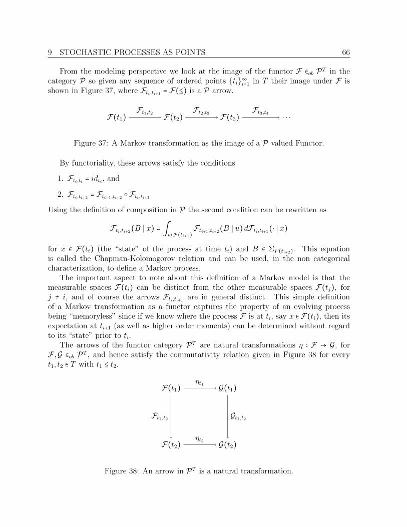
9 STOCHASTIC PROCESSES AS POINTS 66
From the modeling perspective we look at the image of the functor F ∈ob PT in thecategory P so given any sequence of ordered points ti∞i=1 in T their image under F isshown in Figure 37, where Fti,ti+1 = F(≤) is a P arrow.
F(t1) F(t2) F(t3) . . .Ft1,t2 Ft2,t3 Ft3,t4
Figure 37: A Markov transformation as the image of a P valued Functor.
By functoriality, these arrows satisfy the conditions
1. Fti,ti = idti , and
2. Fti,ti+2 = Fti+1,ti+2 Fti,ti+1Using the definition of composition in P the second condition can be rewritten as
Fti,ti+2(B ∣ x) = ∫u∈F(ti+1)
Fti+1,ti+2(B ∣ u)dFti,ti+1(⋅ ∣ x)
for x ∈ F(ti) (the “state” of the process at time ti) and B ∈ ΣF (ti+2). This equationis called the Chapman-Kolomogorov relation and can be used, in the non categoricalcharacterization, to define a Markov process.
The important aspect to note about this definition of a Markov model is that themeasurable spaces F(ti) can be distinct from the other measurable spaces F(tj), forj ≠ i, and of course the arrows Fti,ti+1 are in general distinct. This simple definitionof a Markov transformation as a functor captures the property of an evolving processbeing “memoryless” since if we know where the process F is at ti, say x ∈ F(ti), then itsexpectation at ti+1 (as well as higher order moments) can be determined without regardto its “state” prior to ti.
The arrows of the functor category PT are natural transformations η ∶ F → G, forF ,G ∈ob PT , and hence satisfy the commutativity relation given in Figure 38 for everyt1, t2 ∈ T with t1 ≤ t2.
F(t1)
F(t2)
G(t1)
G(t2)
Ft1,t2
ηt1
ηt2
Gt1,t2
Figure 38: An arrow in PT is a natural transformation.
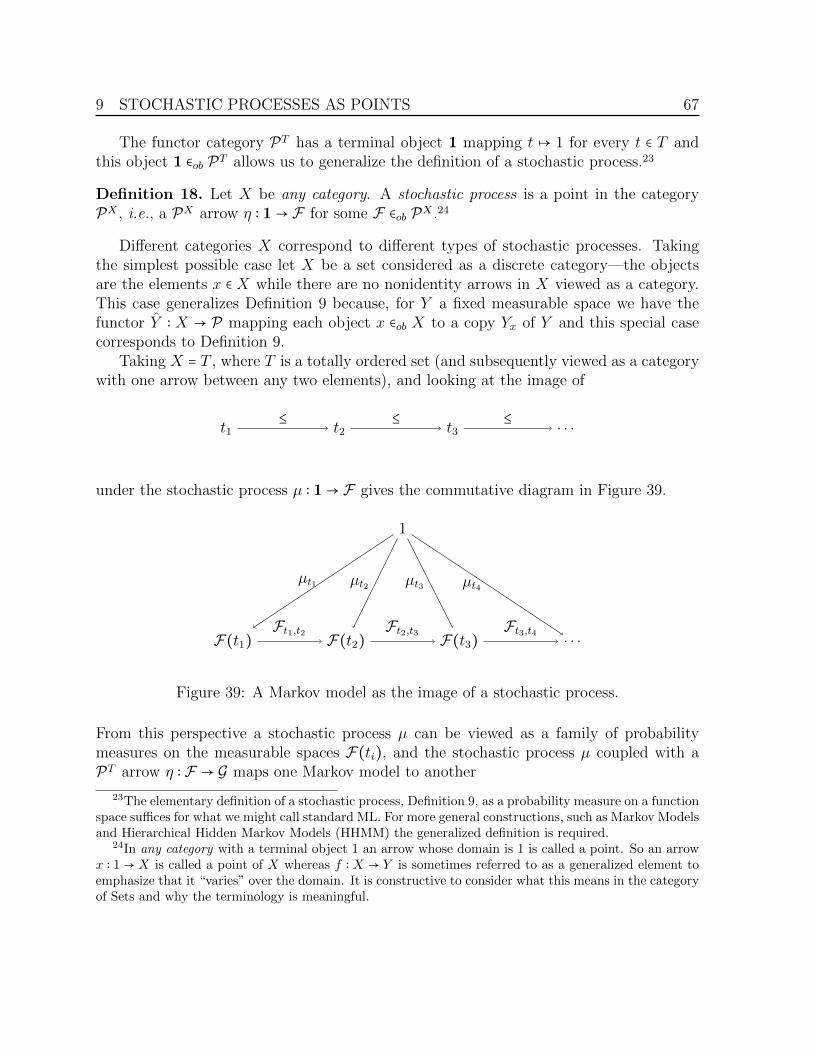
9 STOCHASTIC PROCESSES AS POINTS 67
The functor category PT has a terminal object 1 mapping t ↦ 1 for every t ∈ T andthis object 1 ∈ob PT allows us to generalize the definition of a stochastic process.23
Definition 18. Let X be any category. A stochastic process is a point in the categoryPX , i.e., a PX arrow η ∶ 1→ F for some F ∈ob PX .24
Different categories X correspond to different types of stochastic processes. Takingthe simplest possible case let X be a set considered as a discrete category—the objectsare the elements x ∈ X while there are no nonidentity arrows in X viewed as a category.This case generalizes Definition 9 because, for Y a fixed measurable space we have thefunctor Y ∶ X → P mapping each object x ∈ob X to a copy Yx of Y and this special casecorresponds to Definition 9.
Taking X = T , where T is a totally ordered set (and subsequently viewed as a categorywith one arrow between any two elements), and looking at the image of
t1 t2 t3 . . .≤ ≤ ≤
under the stochastic process µ ∶ 1→ F gives the commutative diagram in Figure 39.
1
F(t1) F(t2) F(t3) . . .Ft1,t2 Ft2,t3 Ft3,t4
µt1 µt2 µt3 µt4
Figure 39: A Markov model as the image of a stochastic process.
From this perspective a stochastic process µ can be viewed as a family of probabilitymeasures on the measurable spaces F(ti), and the stochastic process µ coupled with aPT arrow η ∶ F → G maps one Markov model to another
23The elementary definition of a stochastic process, Definition 9, as a probability measure on a functionspace suffices for what we might call standard ML. For more general constructions, such as Markov Modelsand Hierarchical Hidden Markov Models (HHMM) the generalized definition is required.
24In any category with a terminal object 1 an arrow whose domain is 1 is called a point. So an arrowx ∶ 1 → X is called a point of X whereas f ∶ X → Y is sometimes referred to as a generalized element toemphasize that it “varies” over the domain. It is constructive to consider what this means in the categoryof Sets and why the terminology is meaningful.

9 STOCHASTIC PROCESSES AS POINTS 68
1
F(t1) F(t2) F(t3) . . .
G(t1) G(t2) G(t3) . . .
Ft1,t2 Ft2,t3 Ft3,t4
Gt1,t2 Gt2,t3 Gt3,t4
µt1 µt2 µt3 µt4
ηt1,t2 ηt2,t3 ηt3,t4
One can also observe that GPs can be defined using this generalized definition of astochastic process. For X a measurable space it follows for any finite subset X0 ⊂ X wehave the inclusion map ι ∶ X0 X which is a measurable function, using the subspaceσ-algbra for X0, and we are led back to Diagram 14 with the stochastic process P ∶ 1→ Y ,where Y is as defined in the paragraph above following Definition 18, which satisfies theappropriate restriction property defining a GP.
These simple examples illustrate that different stochastic processes can be obtained byeither varying the structure of the category X and/or by placing additional requirementson the projection maps, e.g., requiring the projections be normal distributions on finitesubspaces of the exponent category X.
9.2 Hidden Markov Models
To bring in the Bayesian aspect of Markov models it is necessary to consider the mea-surement process associated with a sequence as in Figure 39. In particular, consider thestandard diagram
1
F(t1) Yt1
µt1
St1
dt1
which characterizes a Bayesian model, where Yt1 is a copy of a Y which is a data mea-surement space, St1 is interpreted as a measurement model and dt1 is an actual datameasurement on the “state” space F(t1). This determines an inference map It1 so that

10 FINAL REMARKS 69
given a measurement dt1 the posterior probability on F(t1) is It1 dt1 . Putting the twomeasurement models together with the Markov transformation model F we obtain thefollowing diagram in Figure 40.
1
F(t1) F(t2)
Yt1 Yt2
µt1
Ft1,t2
St1 It1dt1
µt1 = I dt1Ft1,t2 µt1
St2 It2
Figure 40: The hidden Markov model viewed in P.
This is the hidden Markov process in which given a prior probability µt1 on the spaceFt1 we can use the measurement dt1 to update the prior to the posterior µt1 = It1 dt1 onF(t1). The posterior then composes with Ft1,t2 to give the prior Ft1,t2 µt1 on F(t2), andnow the process can be repeated indefinitely. The Kalman filter is an example in which theMarkov map Ft1,t2 describe the linear dynamics of some system under consideration (asin tracking a satellite), while the sampling distributions St1 model the noisy measurementprocess which for the Kalman filter is Gaussian additive noise. Of course one can easilyreplace the linear dynamic by a nonlinear dynamic and the Gaussian additive noise modelby any other measurement model, obtaining an extended Kalman filter, and the aboveform of the diagram does not change at all, only the P maps change.
10 Final Remarks
In closing, we would like to make a few comments on the use of category theory for ML,where the largest potential payoff lies in exploiting the abstract framework that categoricallanguage provides. This section assumes a basic familiarity with monads and should beviewed as only providing conceptual directions for future research which we believe arerelevant for the mathematical development of learning systems. Further details on thetheory of monads can be found in most category theory books, while the basics as theyrelate to our discussion below can be found in our previous paper [6], in which we providethe simplest possible example of a decision rule on a discrete space.
Seemingly all aspects of ML including Dirichlet distributions and unsupervised learn-ing (clustering) can be characterized using the category P. As an elementary example,

10 FINAL REMARKS 70
mixture models can be developed by consideration of the space of all (perfect) probabilitymeasures PX on a measurable space X endowed with the coarsest σ-algebra such thatthe evaluation maps evB ∶ PX → [0,1] given by evB(P ) = P (B), for all B ∈ ΣX , aremeasurable. This actually defines the object mapping of a functor P ∶ P →Meas whichsends a measurable space X to the space PX of probability measures on X. On arrows,P sends the P-arrow f ∶ X → Y to the measurable function Pf ∶ PX → PY definedpointwise on ΣY by
Pf(P )(B) = ∫XfB dP.
This functor is called the Giry monad, denoted G, and the Kleisli category K(G) of theGiry monad is equivalent to P.25 The reason we have chosen to present the materialfrom the perspective of P rather that K(G) is that the existing literature on ML usesMarkov kernels rather than the equivalent arrows in K(G). The Giry monad determinesthe nondeterministic P mapping
XPX εX
given by εX(P,B) = evB(P ) = P (B) for all P ∈ P(X) and all B ∈ ΣX . Using thisconstruction, any probability measure P on PX then yields a mixture of probabilitymeasures on X through the composite map
1
XPX
P
εX
εX P = A mixture model.
We have briefly introduced the Kleisli category K(G) (≅ P) because it is a subcategoryD of the Eilenberg–Moore category of G-algebras, which we call the category of decisionrules,26 because the objects of this category are Meas arrows r ∶ PX → X sending aprobability measure P on X to an actual element of X satisfying some basic propertiesincluding r(δx) = x. Thus r acts as a decision rule converting a probability measure onX to an actual element of X and, if P is deterministic, takes that measure to the pointx ∈ X of nonzero measure.27 Decision theory is generally presented from the perspectiveof taking probability measures on X and, usually via a family of loss functions θ ∶X → R,
25See Giry[14] for the basic definitions and equivalence of these categories.26Doberkat [8] has analyzed the Kleisli category under the condition that the arrows are not only
measurable but also continuous. This is an unnecessary assumption, resulting in all finite spaces havingno decision rules, though his considerable work on this category K(G) provides much useful insight aswell as applications of this category.
27Measurable spaces are defined only up to isomorphism, so that if two elements x, y ∈ X are nondis-tinguishable in terms of the σ-algebra, meaning there exist no measurable set A ∈ ΣX such that x ∈ Aand y /∈ A, then δx = δy and we also identify x with y.

11 APPENDIX A: INTEGRALS OVER PROBABILITY MEASURES. 71
making a selection among a family of possible choices θ ∈ Θ where Θ is some measurablespace rather than X. However, it can clearly be viewed from this more basic viewpoint.
The largest potential payoff in using category theory for ML and related applicationsappears to be in integrating decision theory with probability theory, expressed in terms ofthe category D, which would provide a basis for an automated reasoning system. Whilethe Bayesian framework presented in this paper can fruitfully be exploited to constructestimation of unknown functions it still lacks the ability to make decisions of any kind.Even if we were to invoke a list of simple rules to make decisions the category P istoo restrictive to implement these rules. By working in the larger category of decisionrules D, it is possible to implement both the Bayesian reasoning presented in this workas well as decision rules as part of larger reasoning system. Our perspective on thisproblem is that Bayesian reasoning in general is inadequate—not only because it lacksthe ability to make decisions—but because it is a passive system which “waits around”for additional measurement data. An automated reasoning system must take self directedaction as in commanding itself to “swivel the camera 45 degrees right to obtain necessaryadditional information”, which is a (decision) command and control component whichcan be integrated with Bayesian reasoning. An intelligent system would in addition,based upon the work of Rosen [21], in which he employed categorical ideas, possess ananticipatory component. While he did not use the language of SMCC it is clear thisaspect was his intention and critical in his method of modeling intelligent systems, andwithin the category D this additional aspect can also be modeled.
11 Appendix A: Integrals over probability measures.
The following three properties are the only three properties used throughout the paperto derive the values of integrals defined over probability measures.
1. The integral of any measurable function f ∶ X → R with respect to a dirac measuresatisfies
∫u∈X
f(u)dδx = f(x).
This is straightforward to show using standard measure theoretic arguments.
2. Integration with respect to a push forward measure can be pulled back. Supposef ∶ X → Y is any measurable function, P is a probability measure on X, andφ ∶ Y → R is any measurable function. Then
∫y∈Y
φ(y)d(Pf−1) = ∫x∈X
φ(f(x))dP
To prove this simply show that it holds for φ = 1B, the characteristic function atB, then extend it to any simple function, and finally use the monotone convergencetheorem to show it holds for any measurable function.

13 REFERENCES 72
3. Suppose f ∶ X → Y is any measurable function and P is a probability measure onX. Then
∫x∈X
δf(B ∣ x)dP = ∫x∈X
1B(f(x))dP = P (f−1(B))
This is a special case of case (2) with φ = 1B.
12 Appendix B: The weak closed structure in PHere is a simple illustration of the weak closed property of P using finite spaces. LetX = 2 = 0,1 and Y = a, b, c, both with the powerset σ-algebra. This yields thepowerset σ-algebra on Y X and each function can be represented by an ordered pair, suchas (b, c) denoting the function f(1) = b and f(2) = c. Define two probability measuresP,Q on Y X by
P ((b, c)) = .5 = P ((c, b))Q((b, b)) = .5 = Q((c, c))
and both measures having a value of 0 on all other singleton measurable sets. Both ofthese probability measures on Y X yield the same conditional probability measure
(X,ΣX) (Y,ΣY )P = Q
sinceP (a∣1) = 0 = Q(a∣1)P (b∣1) = .5 = Q(b∣1)P (c∣1) = .5 = Q(c∣1)
andP (a∣2) = 0 = Q(a∣2)P (b∣2) = .5 = Q(b∣2)P (c∣2) = .5 = Q(c∣2)
Since P ≠ Q the uniqueness condition required for the closedness property fails and onlythe existence condition is satisfied.
13 References
[1] S. Abramsky, R. Blute, and P. Panangaden, Nuclear and trace ideals in tensored-∗categories. Journal of Pure and Applied Algebra, Vol. 143, Issue 1-3, 1999, pp 3-47.
[2] David Barber, Bayesian Reasoning and Machine Learning, Cambridge UniversityPress, 2012.

13 REFERENCES 73
[3] N. N. Cencov, Statistical decision rules and optimal inference, Volume 53 of Trans-lations of Mathematical Monographs, American Mathematical Society, 1982.
[4] Bob Coecke and Robert Speckens, Picturing classical and quantum Bayesian in-ference, Synthese, June 2012, Volume 186, Issue 3, pp 651-696. http://link.
springer.com/article/10.1007/s11229-011-9917-5
[5] David Corfield, Category Theory in Machine Learning, n-category cafe blog.http://golem.ph.utexas.edu/category/2007/09/category_theory_in_
machine_lea.html
[6] Jared Culbertson and Kirk Sturtz, A Categorical Foundation for Bayesian Proba-bility, Applied Categorical Structures, 2013. http://link.springer.com/article/10.1007/s10485-013-9324-9.
[7] R. Davis, Gaussian Processes, http://www.stat.columbia.edu/~rdavis/papers/VAG002.pdf
[8] E.E. Doberkat, Kleisi morphism and randomized congruences for the Giry monad, J.Pure and Applied Algebra, Vol. 211, pp 638-664, 2007.
[9] R.M. Dudley, Real Analysis and Probability, Cambridge Studies in Advanced Math-ematics, no. 74, Cambridge University Press, 2002
[10] R. Durrett, Probability: Theory and Examples, 4th ed., Cambridge University Press,New York, 2010.
[11] A.M. Faden. The Existence of Regular Conditional Probabilities: Necessary andSufficient Conditions. The Annals of Probability, 1985, Vol. 13, No. 1, 288-298.
[12] Brendan Fong, Causal Theories: A Categorical Perspective on Bayesian Networks.Preprint, April 2013. http://arxiv.org/pdf/1301.6201.pdf
[13] Tobias Fritz, A presentation of the category of stochastic matrices, 2009. http:
//arxiv.org/pdf/0902.2554.pdf
[14] M. Giry, A categorical approach to probability theory, in Categorical Aspects ofTopology and Analysis, Vol. 915, pp 68-85, Springer-Verlag, 1982.
[15] E.T. Jaynes, Probability Theory: The Logic of Science, Cambridge University Press,2003.
[16] F.W. Lawvere, The category of probabilistic mappings. Unpublished seminar notes1962.
[17] F.W. Lawvere, Bayesian Sections, private communication, 2011.

13 REFERENCES 74
[18] X. Meng, Categories of convex sets and of metric spaces, with applications to stochas-tic programming and related areas, Ph.D. Thesis, State University of New York atBuffalo, 1988.
[19] Kevin Murphy, Machine Learning: A Probabilistic Perspective, MIT Press, 2012.
[20] C.E. Rasmussen and C.K.I.. Williams, Gaussian Processes for Machine Learning.MIT Press, 2006.
[21] Robert Rosen, Life Itself, Columbia University Press, 1991.
[22] V.A. Voevodskii, Categorical probability, Steklov Mathematical Institute Semi-nar, Nov. 20, 2008. http://www.mathnet.ru/php/seminars.phtml?option_lang=eng&presentid=259.
Jared Culbertson Kirk SturtzRYAT, Sensors Directorate Universal MathematicsAir Force Research Laboratory, WPAFB Vandalia, OH 45377Dayton, OH 45433 [email protected]@us.af.mil