bayesian modelling and analysis of utility-based ...houldinb/home_files/zhou_thesis.pdf · bayesian...
TRANSCRIPT

Bayesian Modelling and Analysis of
Utility-based Maintenance for
Repairable Systems
A thesis submitted to the University of Dublin, Trinity College
in partial fulfillment of the requirements for the degree of
Doctor of Philosophy
Department of Statistics, Trinity College Dublin
September 2016
Shuaiwei Zhou


I dedicate this thesis to my wonderful and supportive parents


Declaration
I declare that this thesis has not been submitted as an exercise for a degree at this
or any other university and it is entirely my own work.
I agree to deposit this thesis in the University’s open access institutional repository
or allow the Library to do so on my behalf, subject to Irish Copyright Legislation and
Trinity College Library conditions of use and acknowledgement.
The copyright remains solely with the author, Shuaiwei Zhou.
Shuaiwei Zhou
Dated: September 12, 2016


Abstract
This thesis focuses on modelling and inference for maintenance systems for the pur-
pose of utility optimisation. Providing standardised notation throughout, we first
demonstrate the motivation for investigating the problem of modelling and inference
for maintenance systems and briefly state the problems which are to be explored. The
definitions and terminology, which are also used within the general domains of science
and engineering, have been presented in terms of statistical representation.
We propose a Bayesian method to optimise the utility of a two phase maintenance
system sequentially by dynamic programming method. In particular, the parameters
of the failure distribution for the system of interest are analysed within the Bayesian
framework. Utility-based maintenance is modelled in several modified models, in-
cluding imperfect preventive maintenance, time value of money effect in maintenance,
maintenance for systems with discrete failure time distributions, maintenance for par-
allel redundant systems, of which all follow numerical examples. A hybrid approach
combining myopic and dynamic programming method is proposed to solve multi-phase
maintenance systems.
The Bayesian dynamic programming is carried out through the gridding approach
to solve the issue arising from nested series of maximisations and integrations over
a highly non-linear space. The core of gridding method, the increment is studied
extensively. We also utilise and modify the approach proposed by Baker (2006) to
analyse the effect of risk aversion on the variability of system in cash flows.
The potential generalisation of the current models has been discussed and the future
work concerning complicated models and efficient computation methods have also been
indicated.
vii

viii

Acknowledgements
I would like to express my utmost and sincere gratitude to my two wonderful super-
visors, Professor Simon P. Wilson and Professor Brett Houlding, for their invaluable
guidance and constant devotion to me during my PhD research. No matter how stupid
the questions I asked or how naıve I was, they were always extremely patient to explain
and explore potential ideas with me.
Within the discipline of statistics, I would like acknowledge the kind help and
interesting discussions with the professors in our department and beyond, in particular
Myra O’Regan, John Hasslet, Eamonn Mullins and Elizabeth Heron. My memorable
PhD journey has been thankfully shared with fellow researchers who are Jason Wyse,
Louis Aslett, Susanne Schimitz, Arnab Bhattacharya, Tiep Mai, Arthur White, Gernot
Roetzer and Angela McCourt. I have been fortunate to have wonderful friendships
with Sean O’Riordain, Cristina De Persis, Thinh Doan, Donnacha Bolger and Shane
O’Meachair. My appreciation also goes to Charles McLaughlin and Michael Kelly with
their generous help during my PhD life in Ireland.
I am also indebted to my parents, and my brother and his wife, for their incredible
encouragement and support. Xiaoyao and Xiaonan, who burst onto the scene during
my undergraduate and postgraduate time, makes me proud of being a happy uncle.
The generous support of a four-year scholarship by the China Scholarship Council
and a three-year studentship by the University of Dublin made it all feasible.
Shuaiwei Zhou
Trinity College, Dublin
September 2016
ix

x

Abbreviations
ARA Absolute Risk Aversion
CARA Constant Absolute Risk Aversion
CBM Condition-based Maintenance
CDF Cumulative Distribution Function
CE Certainty Equivalent
CHF Cumulative Hazard Function
CM Corrective Maintenance
CR Cost Rate
CRRA Constant Relative Risk Aversion
DARA Decreasing Absolute Risk Aversion
DP Dynamic Programming
DRRA Decreasing Relative Risk Aversion
GA Genetic Algorithm
H-M-DP Hybrid Myopic Dynamic Programming
IARA Increasing Absolute Risk Aversion
IID Independent and Identically Distributed
IPM Imperfect Preventive Maintenance
IRRA Increasing Relative Risk Aversion
PDF Probability Density Function
PM Preventive Maintenance
PMF Probability Mass Function
PPM Perfect Preventive Maintenance
RRA Relative Risk Aversion
SA Simulated Annealing
xi

xii

Contents
Abstract vii
Acknowledgements ix
Abbreviations xi
List of Tables xvii
List of Figures xxi
Chapter 1 Introduction 1
1.1 Background and Motivation . . . . . . . . . . . . . . . . . . . . . . . . 1
1.2 Structure and Main Contributions . . . . . . . . . . . . . . . . . . . . . 3
Chapter 2 Repairable Systems and Maintenance 5
2.1 Repairable Systems . . . . . . . . . . . . . . . . . . . . . . . . . . . . . 5
2.1.1 Basic Terminology and Examples . . . . . . . . . . . . . . . . . 5
2.1.2 Reliability Measures . . . . . . . . . . . . . . . . . . . . . . . . 6
2.1.3 Classical Failure Distributions . . . . . . . . . . . . . . . . . . . 9
2.2 Maintenance Modelling . . . . . . . . . . . . . . . . . . . . . . . . . . . 13
2.2.1 Maintenance Policies . . . . . . . . . . . . . . . . . . . . . . . . 14
2.2.2 Maintenance Effectiveness . . . . . . . . . . . . . . . . . . . . . 16
2.2.3 Sequential Maintenance . . . . . . . . . . . . . . . . . . . . . . 19
2.3 Maintenance Optimisation . . . . . . . . . . . . . . . . . . . . . . . . . 20
2.3.1 Optimisation Approaches . . . . . . . . . . . . . . . . . . . . . . 20
2.3.2 Optimisation Objectives . . . . . . . . . . . . . . . . . . . . . . 22
xiii

Chapter 3 Statistical Methodology and Utility 25
3.1 Bayesian Modelling . . . . . . . . . . . . . . . . . . . . . . . . . . . . . 25
3.1.1 Likelihood function . . . . . . . . . . . . . . . . . . . . . . . . . 27
3.1.2 Prior distribution . . . . . . . . . . . . . . . . . . . . . . . . . . 28
3.1.3 Posterior analysis . . . . . . . . . . . . . . . . . . . . . . . . . . 30
3.1.4 Hierarchical Bayesian models . . . . . . . . . . . . . . . . . . . 31
3.1.5 Bayesian method in maintenance . . . . . . . . . . . . . . . . . 33
3.2 Dynamic Programming . . . . . . . . . . . . . . . . . . . . . . . . . . . 35
3.2.1 An Elementary Example . . . . . . . . . . . . . . . . . . . . . . 35
3.2.2 Characteristics . . . . . . . . . . . . . . . . . . . . . . . . . . . 40
3.2.3 Formalisation under Uncertainty . . . . . . . . . . . . . . . . . 42
3.3 Utility Theory . . . . . . . . . . . . . . . . . . . . . . . . . . . . . . . . 43
3.3.1 Utility Functions and Probabilities . . . . . . . . . . . . . . . . 44
3.3.2 Expected Utility . . . . . . . . . . . . . . . . . . . . . . . . . . 46
3.3.3 Risk Aversion . . . . . . . . . . . . . . . . . . . . . . . . . . . . 48
3.3.4 Utility in Maintenance . . . . . . . . . . . . . . . . . . . . . . . 50
Chapter 4 Sequential Preventive Maintenance 53
4.1 The Problem Setting . . . . . . . . . . . . . . . . . . . . . . . . . . . . 54
4.2 Utility Functions . . . . . . . . . . . . . . . . . . . . . . . . . . . . . . 57
4.3 Modelling Maintenance . . . . . . . . . . . . . . . . . . . . . . . . . . . 59
4.3.1 Myopic Modelling . . . . . . . . . . . . . . . . . . . . . . . . . . 59
4.3.2 Stochastic Dynamic Programming . . . . . . . . . . . . . . . . . 61
4.3.3 Bayesian Weibull Modelling . . . . . . . . . . . . . . . . . . . . 62
4.3.3.1 One-Phase System . . . . . . . . . . . . . . . . . . . . 68
4.3.3.2 Two-Phase System . . . . . . . . . . . . . . . . . . . . 68
4.3.4 Gridding Approach . . . . . . . . . . . . . . . . . . . . . . . . . 72
4.3.5 Pseudocode . . . . . . . . . . . . . . . . . . . . . . . . . . . . . 82
4.4 Numerical Examples . . . . . . . . . . . . . . . . . . . . . . . . . . . . 84
4.4.1 PPM for Two-Phase System . . . . . . . . . . . . . . . . . . . . 84
4.4.2 Simulation . . . . . . . . . . . . . . . . . . . . . . . . . . . . . . 90
xiv

Chapter 5 Sequential Maintenance Extension 93
5.1 Imperfect Maintenance . . . . . . . . . . . . . . . . . . . . . . . . . . . 93
5.2 Time Value of Money . . . . . . . . . . . . . . . . . . . . . . . . . . . . 98
5.3 Maintenance in Discrete Time . . . . . . . . . . . . . . . . . . . . . . . 100
5.4 Maintenance for Parallel Systems . . . . . . . . . . . . . . . . . . . . . 103
5.5 PPM under failure time distribution assumptions . . . . . . . . . . . . 105
5.6 Hybrid Myopic-Dynamic Programming . . . . . . . . . . . . . . . . . . 108
5.7 Sensitivity Analysis . . . . . . . . . . . . . . . . . . . . . . . . . . . . . 117
5.7.1 Gridding Increments . . . . . . . . . . . . . . . . . . . . . . . . 117
5.7.2 Cost Structure . . . . . . . . . . . . . . . . . . . . . . . . . . . 121
5.7.3 Prior Sensitivity . . . . . . . . . . . . . . . . . . . . . . . . . . . 122
5.7.4 Utility Function Forms . . . . . . . . . . . . . . . . . . . . . . . 123
5.8 Parallel Computing . . . . . . . . . . . . . . . . . . . . . . . . . . . . . 125
Chapter 6 Risk Aversion in Maintenance 127
6.1 Utility Functions . . . . . . . . . . . . . . . . . . . . . . . . . . . . . . 127
6.2 Risk-averse Maintenance Modelling . . . . . . . . . . . . . . . . . . . . 129
6.3 Numerical Examples . . . . . . . . . . . . . . . . . . . . . . . . . . . . 131
6.4 Discussions . . . . . . . . . . . . . . . . . . . . . . . . . . . . . . . . . 132
Chapter 7 Conclusions and Future Work 133
7.1 Conclusions . . . . . . . . . . . . . . . . . . . . . . . . . . . . . . . . . 133
7.2 Applications . . . . . . . . . . . . . . . . . . . . . . . . . . . . . . . . . 134
7.3 Outlook . . . . . . . . . . . . . . . . . . . . . . . . . . . . . . . . . . . 135
Appendix A Glossary 137
Appendix B Mathematical Proofs 139
B.1 Iso-elastic Utility Functions . . . . . . . . . . . . . . . . . . . . . . . . 139
B.2 Negative Exponential Utility Functions . . . . . . . . . . . . . . . . . . 140
B.3 Certainty Equivalent . . . . . . . . . . . . . . . . . . . . . . . . . . . . 140
B.4 Risk Aversion . . . . . . . . . . . . . . . . . . . . . . . . . . . . . . . . 141
Appendix C Computational Notes 143
xv

xvi

List of Tables
2.1 State Assumptions after Maintenance . . . . . . . . . . . . . . . . . . . 17
3.1 Number of failed students for a course with 4 sessions and 6 available
demonstrators. . . . . . . . . . . . . . . . . . . . . . . . . . . . . . . . 36
3.2 Dynamic Programming Example: Stage 4. . . . . . . . . . . . . . . . . 37
3.3 Dynamic Programming Example: Stage 3. . . . . . . . . . . . . . . . . 38
3.4 Dynamic Programming Example: Stage 2. . . . . . . . . . . . . . . . . 38
3.5 Dynamic Programming Example: Stage 1. . . . . . . . . . . . . . . . . 39
3.6 Properties of Utility Functions . . . . . . . . . . . . . . . . . . . . . . . 49
4.1 Optimal corrective maintenance (CM) time and corresponding expected
cost for each chance node based on dynamic programming and myopic
methods. Bracketed figures are failure time Tf1 with respect to T ∗m1and
T ∗m2, numbers in brackets representing corresponding failure times. . . . 86
4.2 Optimum Perfect Preventive Maintenance (PPM) time through different
optimisation objectives, i.e., expected cost and expected utility for each
chance node based on dynamic programming method. Bracketed figures
are failure time Tf1 with respect to Tm1 and Tm2 , numbers in brackets
representing corresponding failure times. . . . . . . . . . . . . . . . . . 87
4.3 Optimal perfect preventive maintenance (PPM) time and corresponding
expected utility for chance node CN1 by dynamic programming condi-
tioning on various risk aversion parameter η of an exponential utility
function. . . . . . . . . . . . . . . . . . . . . . . . . . . . . . . . . . . . 88
4.4 Two-Phase Maintenance System Simulation Results. . . . . . . . . . . 91
xvii

5.1 Optimal Imperfect Preventive Maintenance (IPM) time and correspond-
ing expected cost for chance nodes CN1 and CN22 conditioning on vari-
ous PM power parameter β based on dynamic programming and myopic
methods. . . . . . . . . . . . . . . . . . . . . . . . . . . . . . . . . . . . 97
5.2 Optimal Perfect Preventive Maintenance (PPM) time and corresponding
expected cost rate for chance node CN1 conditioning on various time
effect parameter r based on dynamic programming. indicates the
cost rate comparison to its previous one. . . . . . . . . . . . . . . . . . 99
5.3 Optimal perfect preventive maintenance (PPM) time and corresponding
expected cost for chance node CN1 by dynamic programming condition-
ing on various parameter p of a discrete Weibull failure distribution. . . 102
5.4 Optimal perfect preventive maintenance (PPM) time and corresponding
expected cost rate for each chance node by dynamic programming for
one-unit systems and two-unit redundant parallel systems. Bracketed
figures are failure time Tf1 with respect to Tm1 and Tm2 , numbers in
brackets representing corresponding failure times. . . . . . . . . . . . . 104
5.5 Optimal Perfect Preventive Maintenance (PPM) time and corresponding
expected cost rate for each chance node by dynamic programming based
on Weibull and gamma failure time assumptions. Bracketed figures are
failure time Tf1 with respect to Tm1 and Tm2 , numbers in brackets rep-
resenting corresponding failure times. . . . . . . . . . . . . . . . . . . . 107
5.6 Optimal Perfect Preventive Maintenance (PPM) time and correspond-
ing expected cost rate of chance nodes CN21 and CN22 for three-phase
maintenance systems based on Hybrid Myopic-Dynamic Programming
and myopic methods. . . . . . . . . . . . . . . . . . . . . . . . . . . . . 115
5.7 Comparison of optimal perfect preventive maintenance (PPM) time and
corresponding expected cost for each chance node based on different in-
crement parameter δ. Bracketed figures are failure time Tf1 with respect
to Tm1 and Tm2 , numbers in brackets representing corresponding failure
times. . . . . . . . . . . . . . . . . . . . . . . . . . . . . . . . . . . . . 118
xviii

5.8 Optimal perfect preventive maintenance (PPM) time and corresponding
expected cost for chance node CN1 conditioning on various increment
parameter δ based on dynamic programming. . . . . . . . . . . . . . . 119
5.9 Optimal perfect preventive maintenance (PPM) time and correspond-
ing expected cost for chance node CN1 conditioning on cost difference
between failure and maintenance based on dynamic programming. . . . 121
5.10 Optimal perfect preventive maintenance (PPM) time and corresponding
expected cost for chance node CN1 conditioning on various prior mean
of parameter θ based on dynamic programming. . . . . . . . . . . . . . 122
5.11 Optimal perfect preventive maintenance (PPM) time and correspond-
ing expected cost for chance node CN1 conditioning on various prior
standard deviation of parameter θ based on dynamic programming. . . 123
5.12 Optimal perfect preventive maintenance (PPM) time and corresponding
expected cost for each chance node by dynamic programming based on
non-Log and Log utility functions. Bracketed figures are failure time
Tf1 with respect to Tm1 and Tm2 , numbers in brackets representing cor-
responding failure times. . . . . . . . . . . . . . . . . . . . . . . . . . . 124
xix

xx

List of Figures
2.1 Comparison of Weibull Distributions with Different Shape Parameters
η: Probability Density Functions (top-left), Cumulative Distribution
Functions (top-right), Survival Functions (bottom-left), Hazard Func-
tions (bottom-right). . . . . . . . . . . . . . . . . . . . . . . . . . . . . 11
2.2 Comparison of Gamma Distributions with Different Shape Parameters
η: Probability Density Functions (top-left), Cumulative Distribution
Functions (top-right), Survival Functions (bottom-left), Hazard Func-
tions (bottom-right). . . . . . . . . . . . . . . . . . . . . . . . . . . . . 13
4.1 Decision Tree for Two-Phase System . . . . . . . . . . . . . . . . . . . 56
4.2 Exponential utility functions with various risk-aversion parameter η. . . 59
4.3 Comparison of truncated normals with various mean (left) and truncat-
ing points (right). . . . . . . . . . . . . . . . . . . . . . . . . . . . . . . 64
4.4 Expectation of Tf (left) and variance of Tf (right) given θ and κ = 1. . 66
4.5 Prior distribution of θ: truncated normal distribution N(2, 1) truncated
at 1. . . . . . . . . . . . . . . . . . . . . . . . . . . . . . . . . . . . . . 66
4.6 Expectation of θ (left) and variance of θ (right) given a and b =∞. . . 67
4.7 Marginal density of Tf1 : fTf1 (tf1) =∫f(tf1 | θ)f(θ) dθ. . . . . . . . . . . 68
4.8 Maintenance Time Optimisation Simplification. . . . . . . . . . . . . . 72
4.9 Prior distribution of θ (left) and marginal distribution of Tf1 (right) by
the gridding method. . . . . . . . . . . . . . . . . . . . . . . . . . . . . 74
4.10 Probability of Tf2 conditioning on tf1 , i.e., pTf2 (tf2 | tf1 = i), where i =
0.1, . . . , 6, by the gridding method. . . . . . . . . . . . . . . . . . . . . 75
4.11 Comparison of pTf1 (tf1) (red) and pTf2 (tf2 | tf1 = i) (green), where i = 0.1,
0.5, 1.0, 1.1, 1.5, 2.0, 2.1, 2.5, 3.0, 3.1, 3.5, 4.0, 4.1, 4.5, 5.0, 5.1, 5.5, 5.9. 76
xxi

4.12 3D scatter plot for maximal probability of Tf2 conditioning on tf1 , i.e.,
max pTf2 (tf2 | tf1), with vertical lines for each point. . . . . . . . . . . . 77
4.13 Maximal probability of Tf2 conditioning on tf1 , i.e., max pTf2 (tf2 | tf1). . 77
4.14 Tf2 that has maximal probability conditioning on tf1 , i.e., arg max pTf2 (tf2 | tf1);
corresponding probabilities (rounded to 2 decimals) shown alongside
dots that represent Tf2 which maximise the probabilities given a spe-
cific tf1 . . . . . . . . . . . . . . . . . . . . . . . . . . . . . . . . . . . . 78
4.15 Maximal probability of Tf2 and the corresponding Tf2 ; corresponding tf1
shown alongside dots. . . . . . . . . . . . . . . . . . . . . . . . . . . . . 79
4.16 Probability of Tf2 conditioning on tf1 > Tm1 , i.e., pTf2 (tf2 | tf1 > Tm1),
where Tm1 = 0.1, . . . , 6, by the gridding method. . . . . . . . . . . . . . 80
4.17 Comparison of pTf1 (tf1) (red) and pTf2 (tf2 | tf1 > Tm1) (green), where
Tm1 = 0.1, 0.5, 1.0, 1.1, 1.5, 2.0, 2.1, 2.5, 3.0, 3.1, 3.5, 4.0, 4.1, 4.5, 5.0,
5.1, 5.5, 5.9. . . . . . . . . . . . . . . . . . . . . . . . . . . . . . . . . . 81
4.18 Expected utilities for two-phase systems at chance nodes CN21, CN22
and CN1 under the dynamic programming method. . . . . . . . . . . . 85
4.19 Expected costs for two-phase systems at chance nodes CN21, CN22 and
CN1 under the dynamic programming method. . . . . . . . . . . . . . 87
4.20 Risk aversion parameter η on utility. . . . . . . . . . . . . . . . . . . . 88
4.21 Optimal Maintenance Decision Tree for Two-Phase Systems. . . . . . . 89
4.22 Posterior probability density of θ conditioning on Tf1(≤ 0.5) and Tf1 >
0.5 compared with prior probability density of θ. . . . . . . . . . . . . . 90
5.1 Comparison of probabilities of Tf2 conditioning on optimal Tm1 obtained
through PPM and IPM. . . . . . . . . . . . . . . . . . . . . . . . . . . 95
5.2 Comparison of probabilities of Tf2 conditioning on observed Tf1 and
implemented imperfect preventive maintenance at Tm1 . . . . . . . . . . 96
5.3 Discrete Weibull Probability Mass Functions (top-left: p = 0.01, θ = 2;
top-right: p = 0.1, θ = 2; bottom-left: p = 0.5, θ = 2; bottom-right:
p = 0.9, θ = 2). . . . . . . . . . . . . . . . . . . . . . . . . . . . . . . . 101
5.4 Marginal Weibull and gamma probabilities of Tf1 , pW (tf1) and pG(tf1)
with same expectation, i.e., E(TWf ) = E(TGf ). . . . . . . . . . . . . . . 106
xxii

5.5 Decision tree for three-phase system with sequential problem with shad-
ing indicating a range of possible outcomes for the preceding chance
node; Box DP-1 and DP-2 show the break into two period problems. . 109
5.6 Comparison of probabilities of Tf2 conditioning on varying Tf1 and op-
timal Tm1 . . . . . . . . . . . . . . . . . . . . . . . . . . . . . . . . . . . 111
5.7 Posterior probability density of θ conditioning on Tf1 ≤ Tm1(0.5) and
Tf1 > Tm1(0.5) compared with prior probability density of θ. . . . . . . 113
5.8 Expected cost rates at chance node CN21 conditioning on tf1 ≤ Tm1
(top-left: tf1 = 0.1, top-right: tf1 = 0.2, middle-left: tf1 = 0.3, middle-
right: tf1 = 0.4 and bottom-left: tf1 = 0.5; and expected cost rates at
chance node CN22 conditioning on tf1 > Tm1 (bottom-right) under the
H-DP-M method. . . . . . . . . . . . . . . . . . . . . . . . . . . . . . . 114
5.9 Optimal Maintenance Decision Tree for Three-Phase Systems . . . . . . 116
5.10 Sensitivity analysis concerning gridding intervals: Compiling time (top-
left); Optimal Maintenance Time (top-right); Expected Cost Rate (bottom-
left); Expected Cost Rate per Compiling Time Unit (bottom-right). . . 120
5.11 Parallel Computing for p(tf2 , tf1) . . . . . . . . . . . . . . . . . . . . . 125
6.1 Certainty-Equivalent with the risk-aversion parameter η under different
operating times. . . . . . . . . . . . . . . . . . . . . . . . . . . . . . . . 131
xxiii

xxiv

Chapter 1
Introduction
1.1 Background and Motivation
In the current climate of globalisation, competition as well as varying demands from
stakeholders, increasing pressure on manufacturing performance has been one of the
main driving forces in the growth of manufacturing industries (Tsang, 2002). From this
point of view maintenance is a significant activity in industrial practice, resulting in the
importance of maintenance optimisation. Maintenance aims to combat the inevitable
degradation of systems over their operational lifetime and keep them in working order.
Therefore, maintenance plays an important role in sustaining and improving systems
availability, which in turn affects the productivity of the system of interest.
Recently, more attention has been directed towards improving and optimising main-
tenance in manufacturing systems as inappropriate maintenance could result in huge
cost and risk (Holmberg et al., 2010). Maintenance costs can reach anywhere between
15% and 70% of production costs (Wang et al., 2008), which also indicates that there
is still a large potential for increasing the productivity in current maintenance prac-
tices. In some industries, a slight improvement in throughput could result in significant
economic impact.
In modern times, the complexity of maintenance systems has increased drastically,
see Duffuaa et al. (2001). This is partly due to modern manufacturing systems which
involve numerous interactions and dependencies between components. It is evident
that analytical and mathematical approaches are limited in solving such complex main-
tenance problems. When it comes to maintenance optimisation methods, sequential
1

analysis is applied to use accumulating evidence to make advantageous early decisions.
In the context of system engineering, this could help save cost and even improve sys-
tem performance. The Bayesian method of sequential analysis is to make decisions that
minimise the expected value of some loss function which can be viewed as a function
of corresponding inputs and outputs, see DeGroot (1970) and Brockwell and Kadane
(2003). In this thesis, we focus the study on Bayesian sequential analysis applied to
maintenance optimisation of repairable systems.
The study of system maintenance has attracted increasing attention in recent years
because of a need from industry for increasing the reliability and availability of systems
whilst decreasing the associated costs. Percy and Kobbacy (1996) pioneered work in
preventive maintenance modelling from a Bayesian perspective. Damien et al. (2007)
analysed a single item maintenance in a Bayesian semi-parametric setting, which solves
the drawbacks of other models failing to capture the true underlying relationships in
the data. However, their analysis is based on a pre-defined finite time horizon, for
example, see Baker (2010); in other words, the maintenance time phases are pre-defined
which is not practical in reality; in our work, on the contrary, the maintenance time
phases are also pre-defined depending on a particular system but random and flexible,
which meets the maintenance scheduling programme. Nonparametric methods have
also been investigated in system maintenance. Gilardoni et al. (2013) use a power-law-
process parametric method by incorporating the nonparametric maximum likelihood
estimate of an intensity function to estimate the optimal preventive maintenance policy.
However, all these approaches fail to consider sequential maintenance which requires
more complicated modelling and longer computation time.
Maintenance based on prognostics is a prior event analysis and action. By means
of incorporating prognostics into the maintenance decision making process, one could
carry out a maintenance forecast based on known characteristics as well as the evalua-
tion of the significant parameters of the item. With regard to maintenance objectives,
as in most of the literature cost-based optimisation framework is taken (Van Horenbeek
et al., 2010). However, focus should not only be on costs as risk preference is simply
ignored if only cost-oriented objective is taken into account. Utility functions used
to measure risk preferences are ubiquitous in economic research. The little published
work that is the exception occurs in warranty and inventory, see Padmanabhan and
2

Rao (1993); Keren and Pliskin (2006). In fact, the field of maintenance and reliability
is a suitable area to apply risk-averse policies because there are numerous cash flows
occurring stochastically. A drawback of taking cost per unit time as a criterion of
optimality is that two policies might then be equally attractive, even if for one of them
the annual maintenance spend were much more variable than that for the other. What
might be seen by some as over-maintenance, in the sense that mean cost per unit time is
not minimised, could be optimal as a risk-averse policy, in which the large unscheduled
losses from failure have such a dis-utility that very frequent maintenance is carried out.
Clearly, a policy that minimised cost per unit time would be unsatisfactory for a main-
tenance engineer who could not convince management that periods of high loss were
an unavoidable part of an optimal long-term policy or for an enterprise that could not
survive because of short-term cash flow problems. Thus, extra maintenance activity is
an insurance policy against large losses occurring over a period.
Models and methodologies proposed in this thesis are primarily suited for large in-
dustrial purposes, for example, an automatic manufacturing system, a robotic process,
or a computer server for the non-life essential services, in which cases failure is neither
rare or frequent, maintenance itself is not cheap or trivial, but failure is a considerable
expense, though not exorbitantly so. Hence, this approach is not suitable to apply to
maintenance of systems with very high risk aversion properties, e.g., a nuclear power
facility, an off-shore oil field, or a life support system. It is also not worthwhile applying
to trivial systems where the computational cost of performing this analysis outweighs
any savings.
1.2 Structure and Main Contributions
The overall research goal of this thesis is to develop a utility-based prognostic mainte-
nance optimisation methodology within a Bayesian statistical framework, which uses
historical information and predictions in remaning lifetime of repairable systems.
The following is an overview of the structure of this thesis along with the main
research contributions.
• Chapter 1 introduces the research background and motivation, and briefly out-
lines the structure and main contributions of the thesis.
3

• Although research background and motivation is given in Chapter 1, Chapter
2 gives a detailed review on maintenance modelling and analyses as well as the
fundamental concepts in systems maintenance, from reliability measures to clas-
sical failure time distributions. We highlight the essential publications which are
highly related to the research questions in this thesis.
• For those beyond the statistical research community, Chapter 3 briefly presents
the Bayesian perspective on modelling, and continues to introduce the founda-
tional concepts of the dynamic programming method as well as utility theory,
which are the maintenance optimisation methodologies in this research.
• Chapter 4 solves the sequential maintenance problem under the policy of perfect
preventive maintenance by a dynamic programming method utilising the idea
proposed by Brockwell and Kadane (2003), whereby a grid is constructed in the
maintenance and failure time space, over which the utility functions of expected
cost per unit time are evaluated. This method has a computation time which is
linear in the number of phases in the sequential problem.
• Chapter 5 extends the previous sequential preventive models to imperfect preven-
tive maintenance, taking account of the time value of money, modelling preventive
maintenance in discrete time setting as well as maintenance for parallel systems,
analysing the effect of failure time distribution assumptions on preventive mainte-
nance time and proposing an adaptive approach to solving multi-phase systems’
maintenance. Sensitivity analysis via the parameters of sequential preventive
maintenance models will also be carried out in the chapter.
• Chapter 6 utilises and modifies the approach proposed by Baker (2006) to inves-
tigate and analyse the effect of risk aversion on the variability of system in cash
flows from a certainty-equivalent point of view.
• Chapter 7 states the major conclusions and contributions of this research and
suggests future work directions.
4

Chapter 2
Repairable Systems and
Maintenance
In this chapter we introduce the difference between non-repairable systems and re-
pairable systems, and classify the maintenance policies and review related modelling
methods.
2.1 Repairable Systems
2.1.1 Basic Terminology and Examples
A repairable system is a system that can be restored to an operating condition by some
repair process instead of replacement of the entire system. For example, an automobile
is a repairable system because most failures, such as the inability to start because of
a bad starter, can be fixed without replacing the entire automobile. Repair does not
have to involve replacement of any parts. For instance, the automobile may fail to start
because of a bad connection with the battery. In this case cleaning the cables and their
connectors with the battery may solve the problem. On the other hand, a light socket
is not considered as a repairable system. The only way to repair a burned-out light is
to replace the bulb; in other words, replace the entire system.
A non-repairable system is one which is discarded after failure. A light bulb is a
non-repairable system for example. Today, with automated production processes being
implemented in industry, many products that used to be repaired after failure are now
5

discarded when they fail. Consider for example a small desk-top fan which can be
purchased for less than 10 euro at a discount shop. When such a unit fails, we would
probably discard it and buy another, because the cost of fixing it is greater than that
of purchasing a new one. Many electrical systems are now non-repairable, or they are
more expensive to repair than to replace.
A few definitions used in repairable systems are given below.
Definition 2.1 Global time Failure of a repairable system is measured in global
time if the failure times are recorded as time since the initial start-up of the system.
Failures in global time will be denoted by X1 < X2 < · · · .
Definition 2.2 Local time Failure times of a repairable system are measured in
local time if the failure times are recorded as time since the previous failure. Failures
in local time will be denoted by T1, T2, . . ..
Local time is mainly used in the following work, unless explicitly stated.
Definition 2.3 Deterioration and Improvement We say that a repairable sys-
tem is deteriorating if the times between failure tend to get shorter with ageing. If the
times between failure tend to increase, then we will say that the system is improving.
2.1.2 Reliability Measures
There are similarities and differences between repairable and non-repairable systems.
A few issues are clarified to understand repairable system behaviour as follows.
For a non-repairable system the lifetime of the system is a random variable. As
there is no repair, the system would be discarded after its one and only failure, and if it
does not have an impact on the performance of a similar system located elsewhere, then
the assumption that different systems have lifetimes that are independent is reasonable.
Also, if many copies of the system were produced by the same manufacturing process,
then it is also reasonable to assume that the system lifetimes have the same distribution.
These two assumptions can be combined into one statement that says the lifetimes are
independent and identically distributed (IID) from some distribution having cumulative
distribution function (CDF) F (x).
6
Definition 2.4 Cumulative Distribution Function The cumulative distribution
function (CDF) of a random variable X is defined to be the function
F (x) = P (X ≤ x).
Since the lifetime must be nonnegative the probability distribution must have pos-
itive probability on the positive axis only. In other words, F (x) = 0 for x < 0.
Definition 2.5 Survival Function The survival function S(x), also called the re-
liability function, is the probability that a system will carry out its mission through time
x.
The survival function evaluated at x is just the probability that the failure time is
beyond time x. Thus the survival function is related to the CDF in the following way:
S(x) = P (X > x) = 1− P (X ≤ x) = 1− F (x). (2.1)
Definition 2.6 Probability Density Function The probability density function
(PDF) is defined to be the derivative of the CDF, provided that the derivative exists.
That is,
f(x) =d
dxF (x) = − d
dxS(x).
Another way to express the PDF is through the limit
f(x) = lim∆→0
F (x+ ∆x)− F (x)
∆x= lim
∆→0
P (x < X ≤ x+ ∆x)
∆x. (2.2)
Another important function related to, but distinct from the PDF, is the hazard
function.
Definition 2.7 Hazard Function The hazard function is
h(x) = lim∆x→0
P (x < X ≤ x+ ∆x |X > x)
∆x. (2.3)
This is the limit of the probability per unit time that a unit fails (for the first and only
time) in a small interval given that it has survived to the beginning of the interval.
Compare the definition of the hazard function h(x) in (2.3) with the result for the pdf
7

given in (2.2). These are nearly the same, except one is a conditional probability and
the other is not.
One property of a PDF is that it must integrate to 1; that is, since we are dealing
with random variables that have all the probability on the nonnegative axis,∫ ∞0
f(x)dx = 1.
The hazard is defined as the limit of a conditional probability, but it is not a conditional
probability density function. The hazard function does not need to integrate to 1, and
in fact, for most distributions we study, the hazard will not integrate to 1 but infinity
(see Cumulative Hazard Function). For a system whose hazard function is increasing,
this means that (in the limit) the probability of failure in a small interval divided by
the length of the interval is increasing with time. Thus if we take a small fixed length
of time, such as one hour, an increasing hazard would mean that the probability of
failing in this one hour, given that the system survived past the start of that hour,
increases with the age of the system. In this case we say that the system is wearing
out. Compare this definition with that of deterioration for a repairable system. We
say that a repairable system deteriorates when the times between failures tend to get
smaller, and we say that a non-repairable system is wearing out if the hazard function
is increasing. A non-repairable system with a decreasing hazard function is said to
experience burn-in. The term “deteriorate” will be reserved for repairable systems
and the term “wear out” will be reserved for non-repairable systems. Similarly, the
terms “improvement” and “burn-in” will be reserved for repairable and non-repairable
systems, respectively. Also note, for a continuous random variable the hazard function
can be defined as
h(x) =f(x)
S(x).
Knowing any one of the pdf f(x), the cdf F (x), the survival function S(x), or the
hazard function h(x) is enough to find all of the others.
Definition 2.8 Cumulative Hazard Function The quantity
H(x) =
∫ t
0
h(x)dx
is called the cumulative hazard function (CHF).
8

As t tends to infinity, i.e., S(x) tends to 0, the cumulative hazard function increases
without bound, which implies that h(x) must not decrease too quickly, otherwise, H(x)
will converge.
2.1.3 Classical Failure Distributions
The next section covers some of the commonly used distributions for lifetime, including
the exponential, the Weibull, and the gamma.
Exponential Distribution
The simplest model for lifetimes is the exponential distribution.
Definition 2.9 Exponential distribution The exponential distribution is a con-
tinuous distribution having pdf
f(x) = λ exp(−λx), x > 0
and cdf
F (x) = P (X ≤ x) =
∫ x
0
λ exp(−λt)dt = 1− exp(−λx), x > 0. (2.4)
We write X ∼ EXP (λ), where λ is often referred to as a rate parameter, to indicate
that the random variable X has an exponential distribution with a CDF given by (2.4).
The mean and variance of the exponential distribution are 1λ
and 1λ2
, respectively. The
most distinctive feature of the exponential distribution is that it is the only continuous
distribution with the memoryless property.
Definition 2.10 Memoryless property A distribution has the memoryless prop-
erty if
P (X > t+ x |X > t) = P (X > x).
In other words, if the distribution has the memoryless property, then for instance, the
probability that an old unit survives one more day will equal the probability that a
brand new unit will survive one day. The memoryless property imposes some strong
assumptions about the way units age.
Another unique feature of the exponential distribution is that it is the only contin-
uous distribution with a constant hazard function.
9

Weibull Distribution
We discuss here the Weibull distribution for several reasons. First, it is probably the
most widely used distribution for lifetimes. Second, if repairs bring a system back
to a good-as-new state and the times between failures X1, X2, . . . are independent,
then the assumption that the times between failures are iid Weibull random variables
may be reasonable because Weibull is a versatile distribution that can take on the
characteristics of other types of distributions.
Definition 2.11 The Weibull distribution has survival function
S(x) = exp−(xα
)η, x > 0. (2.5)
If X is a random variable with this survival function, then we will write X ∼ WEI(η, α),
where η and α are the shape and scale parameters, respectively.
The cdf, pdf and hazard functions are therefore given as follows:
F (x) = 1− S(x) = 1− exp−(xα
)η, x > 0 (2.6)
f(x) = F ′(x) =η
α
(xα
)η−1
exp−(xα
)η, x > 0 (2.7)
h(x) =f(x)
S(x)=
ηα
(xα
)η−1exp
−(xα
)ηexp
−(xα
)η =η
α
(xα
)η−1
, x > 0. (2.8)
The hazard function h is increasing when η > 1 and decreasing when η < 1. When
η = 1, the hazard function is the constant function h(x) = 1/α. Thus, the exponential
distribution is a special case of the Weibull distribution that occurs when η = 1.
10

η=1.8
η=1
η=0.6
1 2 3 4 5x
0.2
0.4
0.6
0.8
1.0
η=1.8
η=1
η=0.6
1 2 3 4 5x
0.2
0.4
0.6
0.8
1.0
CDF
η=1.8
η=1
η=0.6
1 2 3 4 5x
0.2
0.4
0.6
0.8
1.0
Survival
η=1.8
η=1
η=0.6
1 2 3 4 5x
2
4
6
8
Hazard
Figure 2.1: Comparison of Weibull Distributions with Different Shape Parameters
η: Probability Density Functions (top-left), Cumulative Distribution Functions (top-
right), Survival Functions (bottom-left), Hazard Functions (bottom-right).
When the scale parameter α = 1, Figure 2.1 shows a number of Weibull proba-
bility density functions, cumulative distribution functions and corresponding hazard
functions, respectively.
The mean and variance of the Weibull can be expressed in terms of the gamma
function which is defined below.
Definition 2.12 Gamma Function For a > 0 the gamma function is defined to
be
Γ(a) =
∫ ∞0
xa−1e−xdx.
The next theorem gives the mean and variance of the Weibull distribution in terms of
the gamma function.
Proposition 2.1 If X ∼ WEI(η, α), then
E(X) = αΓ
(1 +
1
η
)(2.9)
11

and
V (X) = α2
[Γ
(1 +
2
η
)−(
Γ
(1 +
1
η
))2]
(2.10)
See Rigdon and Basu (2000) for proofs.
Gamma Distribution
The gamma distribution is another useful model for the lifetime of systems.
Definition 2.13 The pdf for the gamma distribution can be written as
f(x) =xη−1
θηΓ(η)exp(−x/θ), x > 0.
We will write X ∼ GAM(η, θ) if the random variable X has this pdf, where η and θ
are the shape and scale parameters, respectively. Another useful form for the gamma
pdf is obtained by substituting 1/λ for θ; this gives
f(x) =ληxη−1
Γ(η)exp(−λx), x > 0. (2.11)
The cdf and the survival function, and hence also the hazard function, cannot be
written in closed form. We can write the cdf as
F (x) =
∫ x
0
ληωη−1
Γ(η)exp(−λω)dω.
If we make the transformation y = λω, then this becomes
F (x) =
∫ λx
0
λη(y/λ)η−1
Γ(η)e−y
1
λdy
=λη
λη−1Γ(η)
1
λ
∫ λx
0
yη−1e−ydy
=1
Γ(η)
∫ λx
0
yη−1e−ydy.
The hazard function is therefore
h(x) =f(x)
1− F (x)
=
ληxη−1
Γ(η)exp(−λx)
1− 1Γ(η)
∫ λx0yη−1e−ydy
.
This hazard function is increasing when η > 1, decreasing when η < 1, and constant
when η = 1, when the corresponding pdf is that of the exponential distribution.
12

η=1.8
η=1
η=0.6
1 2 3 4 5x
0.2
0.4
0.6
0.8
η=1.8
η=1
η=0.6
1 2 3 4 5x
0.2
0.4
0.6
0.8
1.0
CDF
η=1.8
η=1
η=0.6
1 2 3 4 5x
0.2
0.4
0.6
0.8
1.0
Survival
η=1.8
η=1
η=0.6
1 2 3 4 5x
0.5
1.0
1.5
Hazard
Figure 2.2: Comparison of Gamma Distributions with Different Shape Parameters
η: Probability Density Functions (top-left), Cumulative Distribution Functions (top-
right), Survival Functions (bottom-left), Hazard Functions (bottom-right).
When the scale parameter θ = 1, Figure 2.2 shows a number of gamma proba-
bility density functions, cumulative distribution functions and corresponding hazard
functions, respectively.
2.2 Maintenance Modelling
Traditional repairable systems assume a whole range of performance levels, varying
from perfect functioning to complete failure, and assuming the repair is perfect. How-
ever, many manufacturing systems suffer increasing wear with usage, age or deteri-
oration, that is, perfect functioning is not always satisfied. Therefore, maintenance
management, as an important policy for a repairable system, is widely used to keep
systems in good condition, to decrease failures, and increase system availability. Based
on the European standard (EN 13306:2010), a definition of maintenance management
is given as follows:
13

Definition 2.14 Maintenance Management depicts all activities of the manag-
ment that determine the maintenance objectives, strategies and responsibilities, and
implementation of them by such means as maintenance planning, maintenance control,
and the improvement of maintenance activities and economics.
According to the definition above, the major steps to maintenance modelling can
be summarised as:
1. Determine the maintenance objective(s).
2. Define or select maintenance policies according to measures of system perfor-
mance.
3. Plan, control and improve maintenance.
2.2.1 Maintenance Policies
The availability and usability play a crucial part in a system’s performance because
any breakdowns and holdups can seriously impede its performance. At the same time,
idle systems negatively affect the ratio between fixed cost to output. The reduced
output induced by system breakdowns would result in less production as well as less
profitability which can be regarded as an inefficiency for the system. Moreover, complex
systems usually require a significant startup time after an interruption occurs. Possibly
during this period of time, goods that do not meet acceptable levels, e.g., scrap or goods
of minor quality are produced, as a result, one cannot obtain her or his expected profit
since these products cannot be sold or have to be sold at reduced prices. Thus, efficient
operation of a system requires well-scheduled maintenance to avoid interruptions as
much as possible and to recover from breakdowns quickly.
For a manufacturing system, wear-out, ageing and deteriorating will have a negative
impact on the function of the system, which results in the consequence that the system
cannot fulfil its capability. Maintenance is introduced to counteract those negative ef-
fects from an economic point of view. Therefore, maintenance actions plays an essential
role in sustaining and possibly improving a system’s availability, which in return will
improve the productivity of the system considered. In general, maintenance policies
and strategies are commonly categorised into three domains: Corrective Maintenance
(CM), Preventive Maintenance (PM) and Condition based Maintenance (CBM).
14

Corrective maintenance is initiated when the system sees a breakdown which results
in a stop for a system working and induces considerable cost. Corrective maintenance
is usually named repair, restoration or replacement of failed components. This mainte-
nance policy is often applied to systems of which failure is not costly and do not result
in disastrous situations, for components with constant failure rate, e.g., if a failure time
of components is assumed to follow an exponential distribution.
Preventive maintenance is implemented for the purpose of minimising the nega-
tive impact of an unexpected breakdown. Generally speaking, preventive maintenance
usually involves less resource consumption compared to that of corrective maintenance
and it can be designed in the production plans of the system of interest. PM in-
cludes all partial or complete overhauls, such as filter cleaning, oil charging, etc. in
order to prevent a critical failure that is costly before it actually occurs. It can be
seen that preventive maintenance makes sense in the situation when the failure rate
of a unit or component is increasing in time. Unlike CM that is unexpected, preven-
tive maintenance can usually be properly planned and prepared. Although preventive
maintenance is incorporated to prevent critical failures in system designing, sometimes
failure may still be seen. As a result, it is usually suggested to combine both corrective
maintenance and preventive maintenance tasks.
However, when the operation schedules and environmental variables change in prac-
tice, exhaustive or unnecessary use of preventive maintenance can occur. To make
sure that preventive maintenance is taken only when it is required, condition based
maintenance was introduced by incorporating inspections of the system of interest in
pre-determined intervals to determine the system’s operation condition. Depending on
the outcome of an inspection, relevant maintenance tasks can be implemented. It is
worthwhile noting that CBM is sometimes analysed in the field of PM (Manzini et al.,
2010).
The preventive maintenance policies include time based PM (Roux et al., 2008) in
which PM is conducted every t units of time and age based PM (Chen et al., 2006)
where PM is carried out every t units of operating time. There are other alternatives
of preventive maintenance, e.g., for non-repairable systems, group block replacements
where units or components would be replaced if it failed whereas the other working
components would be replaced at pre-determined schedule (Roux et al., 2008).
15

Condition based maintenance has received less attention probably because it is rel-
atively new compared to CM and PM. However, thanks to the fact that the inspection
is less costly, one is encouraged to implement CBM (Xiang et al., 2012). If a system
is designed to serve for a long period, one inspection monitor can be installed if it is
relatively cheaper. Van Horenbeek and Pintelon (2013) proposed a prognostic mainte-
nance by combining CBM with the prediction about the states of components to see
if a threshold is expected to be reached before the following scheduled inspection. If it
does, the component is replaced immediately. Although it can be seen that there is an
increasing application of CBM in practice (Wang et al., 2008), it is less studied in the
literature.
In reviewing the literature, we find limited effort was taken to compare differ-
ent maintenance policies. Xiang et al. (2012) investigated a repairable system un-
der preventive maintenance and condition based maintenance policies and found that
condition-based maintenance is superior to scheduled maintenance paradigm via simu-
lation. Van Horenbeek and Pintelon (2013) studied five different maintenance policies
(i.e., CM, block PM, age based PM, CBM with inspection and CBM under continuous
monitoring) on one machine and their noted effects.
2.2.2 Maintenance Effectiveness
Preventive maintenance comprises all maintenance activities which are not triggered
by a system failure. Not only the mode of maintenance task (preventive maintenance
or corrective maintenance) and its associated maintenance interval impact the failure
rate, but also its level of quality (effectiveness of maintenance task). The state after a
maintenance action is performed on a component is assumed to be: perfect, imperfect,
minimal, worse or worst (Pham and Wang, 1996). See Table 2.1.
16

Maintenance Policy System State Failure Rate
Preventive maintenance The system state is re-
stored to be “as good
as new”
Decreasing of the failure rate
Imperfect maintenance A maintenance action
that restores the
system to a state
somewhere between
“as good as new” and
“as bad as old”
Decreasing of the failure rate
Minimal Maintenance The system state is
“as bad as old”
No effect on the failure rate
Worse Maintenance System is in operat-
ing state worse than
just prior to the main-
tenance action
Increasing of the failure rate
Worst maintenance System breaks down
right after mainte-
nance action
Increasing of the failure rate
Table 2.1: State assumptions after maintenance
Imperfect, worse or worst maintenance can be caused by repairing parts of a system
mistakenly. In addition to one of the best known models proposed by Brown and
Proschan (1983), Pham and Wang (2006) reviewed other approaches to model imperfect
maintenance, such as (p, q) rule, (p(t), q(t)) rule, improvement factor, and virtual age
approach, etc. Briefly, with probability p, the item is restored to the as good as new
state or otherwise to the as bad as old state with probability q = 1 − p. A novel
approach to modelling imperfect preventive mainteannce will be propsed in Chapter 5.
Quality levels of worse and worst maintenance are related to maintenance and repair
induced failures. Preventive maintenance actions, as cleaning or greasing, mitigate the
deterioration effect of some failure mechanics and restore components to a “as good
as new” condition with respect to some failure mechanisms only. All other failure
17

mechanisms will remain unaffected. Hence, Lin et al. (2001) introduced the concept
of two categories of failure mechanisms, maintainable failure mechanisms and non-
maintainable failure mechanisms. Preventive maintenance will affect maintainable fail-
ure mechanisms exclusively, whereas non-maintainable mechanisms remain unaltered.
Zequeira and Berenguer (2005) stated that the maintainable and non-maintainable
failure rates are dependent and restored the system of interest to a condition between
as good as new and as bad as old via their proposed preventive maintenance actions.
In the literature, three approaches for modelling the impact of preventive mainte-
nance on the failure rate have been studied extensively; a failure rate model by Lie
and Chun (1986) and Nakagawa (1986), Nakagawa (1988), an age reduction model by
Canfield (1986) and Malik (1979) and a hybrid model by Lin et al. (2001).
In maintenance modelling, most researchers model a system as a whole unit, with-
out considering the effect of deterioration and failure on the subsystems. On the other
hand, machines were modelled as subsystems by some researchers. Van Horenbeek
and Pintelon (2013) modelled a simplified version only considering one subsystem in
a few machines and analysed the structural and stochastic dependencies. Roux et al.
(2008) evaluated the impact of three maintenance policies under an assumption that a
system has only two independent components. One of the assumptions in maintenance
modelling is assuming all the units or components of a system are identical and inde-
pendent. There are other less rigorous assumptions and we will include some of them
in our research:
• Perfect maintenance: preventive maintenance is assumed to be done perfectly
and it is often referred to as ‘systems are are good as new’ after preventive
maintenance is conducted. In this thesis, perfect preventive maintenance (PPM)
is equivalent to corrective maintenance (CM) in the sense that they have the
same consequence with regard to the state of the system after maintenance.
• Time of implementing maintenance is assumed to be constant and often is even
reduced to be negligible implying that maintenance is carried out instantaneously.
• Costs of all relevant maintenance tasks are assumed to be known as constant and
the cost of CM is always more than that of PM.
• Relevant resources such as spare components are assumed to be sufficient to
18

conduct maintenance.
• System failures are assumed to be detected immediately.
2.2.3 Sequential Maintenance
Under sequential maintenance, systems may be maintained at unequal time intervals,
in contrast to periodic maintenance in which the maintenance interval is fixed and
unique.
Barlow and Proshan (1965) design a sequential maintenance policy for a finite time
span. Under this maintenance policy, the time for which maintenance is scheduled
depends on the time remaining rather than the pre-determined and identical mainte-
nance time. In addition, the next maintenance interval is determined by minimising
the average cost per unit time during the remaining time. Therefore, this policy does
not determine systems’ future maintenance intervals at the initial time of system per-
formance, which adds flexibility and reduces systems costs.
Nguyen and Murthy (1981) model preventive maintenance under a sequential policy
in which a failure needed to be corrected has not occurred by a reference time ti, where ti
is the maximum time that a system should be fully replaced without extra maintenance
after the (i − 1)th repair; in other words, the system is replaced after (k − 1) repairs.
The system is repaired (or replaced at the kth repair) at the time of failure or at time
ti, whichever occurs first.
Nakagawa (1986) propose and compare periodic and sequential preventive mainte-
nance policies for the system with minimal repair at failure and compute the mainte-
nance intervals in a Weibull distribution case, indicating that a sequential preventive
maintenance policy is superior to a periodic one. Schutz et al. (2011) extend previous
research by considering a system performing a wide range of missions over a finite plan-
ning horizon and a dynamic system failure law is taken into account to modelling the
different missions with various characteristics depending on the operational conditions.
Lin et al. (2000) propose general sequential imperfect preventive maintenance models,
in which the effective remaining time of the system would be reduced whilst the hazard
rate would be adjusted after each preventive maintenance. We refer it to as a hybrid
sequential preventive maintenance model because it considers both time reduction and
19

hazard adjustment on systems.
There are also studies by Dieulle et al. (2003) calculating the long-time expected
cost per unit of time via considering if system’s state is above or below a threshold and
assuming deterioration as a gamma process; and Schutz et al. (2011) investigating the
periodic and sequential preventive maintenance policies over a finite planning horizon.
However, due to the highly mathematical formalisation of their modelling, it is not
staightforward to be applied in practice.
2.3 Maintenance Optimisation
2.3.1 Optimisation Approaches
As the complexity of maintenance systems increases, maintenance optimisation meth-
ods have also developed from classical methods to modern or non-traditional methods.
Classical optimisation methods (Rao, 2009) are analytical and use differential cal-
culus to find the optimal value. For example, scatter search (Chen et al., 2006), Nelder-
Mead method (Roux et al., 2008, 2013), cyclic coordinate method (Xiang et al., 2012),
the modified Powell method (Marquez et al., 2003), Fibonacci algorithms (Asadzadeh
and Azadeh, 2014) and local search (Gupta and Lawsirirat, 2006; Triki et al., 2013),
have been applied to simple manufacturing systems. However, it has been criticised
that optimising maintenance through classical methods lacks the analysis of objective
functions and solution space. Thus it poses difficulty in justification of the optimisation
methods.
In order to deal with the complexity increase of maintenance systems, modern
or non-traditional methods have been utilised (Deb, 2005; Rao, 2009). Two modern
optimisation methods are mainly applied, which are Genetic Algorithms (GA) and
Simulated Annealing (SA). In fact the use of SA is only reported in a few articles. In
this sense, exploration of other modern optimisation methods to systems maintenance
problems could be another research branch.
The most reported modern optimisation method in maintenance, GA, is based upon
the process of natural selection in biology and has been applied to various optimisation
problems (Rao, 2009). SA originates from the idea of the annealing process in metal-
lurgy to harden metals. In other words, metals are melted in a high temperature at the
20

beginning and then cooled gradually under a fully controlled environment to obtain
desirable shapes or properties. This method has been used to solve a wide variety of
problems, such as the ones with continuous, discrete and mixed-integer variables (Rao,
2009).
Dynamic programming (DP), see Bellman (1954), is a method of solving a com-
plex problem by breaking it down into series of simpler subproblems (different parts
of the original problem) and then combining the solutions to the subproblems to ob-
tain an overall solution to the original problem. There are two advantages using this
formulation. First, dynamic programming enables computing the optimal solution in
some cases which usually only applies to smaller problems. Due to the curse of di-
mensionality, computing the optimal solution to larger problems cannot be done in
a reasonable and feasible amount of time (Powell, 2007). Second, dynamic program-
ming can produce optimal theoretical results which could indicate the behaviour of the
optimal policy in the proposed models, for example, see Ding et al. (2002).
In a general assumption about state, action and parameter spaces, Rieder (1975)
consider a non-stationary Bayesian dynamic decision model which can be reduced to
a non-Markovian decision model with known transition probabilities. As a pioneer-
ing work in Bayesian dynamic programming, his work provides criteria of optimality
and the existence of Bayes policies. Nicolato and Runggaldier (1999) combine burn-
in, which is used to cope with the problem of “infant mortality” in system running
periods, with identical multi-component systems, and propose a Bayesian dynamic
programming method to make decisions on the optimal maintenance interval and best
burn-in time.
In other words, dynamic programming is an optimisation approach that transforms
a complex problem into a sequence of simpler problems; its essential characteristic is the
multistage nature of the optimisation procedure, which provides a general framework
employed to solve particular aspects of a more general formulation. In the decision
tree problem, we often call it “Roll-Back”, see Ross (1995). As in the problem we
will discuss in the next chapter, we divide the system’s running procedure into a few
stages and based on the information we learn from running the system, we model the
functional form of the system utility and then attempt to maximise it.
The problem addressed in the next chapter is associated with a two-phase sequential
21

problem. We consider the system running from a global perspective, which means we
assume the whole running procedure of the system, and make a decision based on the
optimal utility of the system. On the contrary, myopic decision making means that
we can do local utility optimisation based on the information we previously obtained.
Although we would not obtain the optimal utility for the system, optimisation problems
can be simplified and are also easier to implement in practice, and we can simply regard
it as a “roll-forward” method.
2.3.2 Optimisation Objectives
Cost minimisation is one of the most reported optimisation objectives in maintenance
studies, for example, minimising total cost or expected cost per unit time. Increasing
preventive maintenance cost could result in over-maintenance for systems while increas-
ing hazard rate and its consequences would end up with under-maintenance. Note that
usually corrective maintenance cost is fixed and higher than preventive maintenance
cost (Gupta and Lawsirirat, 2006; Roux et al., 2008; Xiang et al., 2012). However, it is
not sufficient to simply only consider maintenance cost as maintenance is part of sys-
tems and various costs are associated with systems processing. Thus some researchers
have incorporated other costs, in addition to maintenance cost, into maintenance ob-
jectives. For instance, a penalty per unit time for systems unavailability (Alrabghi and
Tiwari, 2013), or the cost resulting from unsatisfactory products (Oyarbide-Zubillaga
et al., 2008).
On the contrast to maintenance cost, Roux et al. (2013) propose maximising sys-
tems availability as the optimisation objective. They argue that it is more justified as
production costs are more dominant in the total cost of systems running. However,
such interpretation would ignore the fact that maintenance costs can be higher than
production costs (Wang et al., 2008).
However, it is suggested to design the objective as maximising production through-
put because maximum system availability does not necessarily guarantee maximum
production throughput (Lei et al., 2010) because a system would not be in a working
state due to various reasons such as lack of raw materials or supporting tools.
On the requirements of different engineering problems, optimising several objec-
tives simultaneously for repairable systems has drawn more attention, e.g., minimising
22

average cost per unit time and maximising systems availability. There are mainly
three ways to realise this aim: firstly, put several objectives into one objective func-
tion, however, this method requires transformation in a universal unit among different
objectives; secondly, assign weights to different objectives based on decision maker’s
preference. Although transformation is not required in this method, the decision maker
has to trade-off among objectives; thirdly, simply solve several objectives simultane-
ously using multi-objective optimisation algorithms, e.g., Oyarbide-Zubillaga et al.
(2008) implement a Non-dominated Sorting Genetic Algorithm to minimise costs as
well as maximise system production profits.
The objective proposed in this thesis is utility-based maintenance. From the main-
tenance engineer’s point of view, by incorporating risk preferences into maintenance
modelling, management of systems could avoid short-term problems such as short-term
cash flow problems by considering optimal long-term policy such as systems availabil-
ity. For example, there are two policies that are equally preferred based on minimising
average cost per unit time, however, it is likely that one of them has more variable
cash flows than the other, which would result in instability.
23

24

Chapter 3
Statistical Methodology and Utility
In operational research and management science we face uncertainty frequently, whether
in the form of uncertain demand for production, uncertain performing time in systems,
or uncertainty about parameters calibrating a simulation model, etc. Despite the fact
that we are facing uncertainty, we usually are able to collect some related information
which could reduce the effects of such uncertainty. This would have two impacts: on
one hand, gathering information helps us make better decisions which could produce
better outcomes; on the other hand, the costs induced by collecting information, such
as time and money spent, or even opportunity cost due to collecting one piece of infor-
mation whereas we could have had another, could increase. How to find the optimal
balance between these benefits and costs is what we are attempting to explore. Two
methods for formulating such problems are Bayesian methods and Dynamic Program-
ming, respectively.
3.1 Bayesian Modelling
In the twentieth century, the so called ‘frequentism’ has dominated the statistical phi-
losophy. Under the framework of the frequentist approach, the hypothetical long term
proportion of the time that an event of interest occurs is expressed via probability and
the parameters of probability models are regarded to be unknown but fixed numeri-
cal quantities. Pearson studied the problems of the frequentist style extensively in the
early twentieth century. One can find most of the foundations for frequentist modelling
and inference in the classical work by Fisher (1922).
25

Bayesian modelling arises earlier than the frequentist methodology actually. It is
being dated back to a thought experiment conducted by Bayes (1763) who threw balls
onto a square table, and to the ‘inverse probability’ found by Laplace (1774) and later
replaced as ‘Bayesian’ in the 1950s by Fisher (Fienberg, 2006). Both Bayes and Fisher
took the uniform prior distribution: it was a outcome of the ball throwing experiment
in Bayes’ case, while it was considered as an intuitive axiom which is a ‘principle of
insufficient reason’ by Fisher. Yet, Bayesian modelling and inference has not drawn
much attention until it reappeared and was recognised in the modern form thanks to
Jeffreys (1939) and Savage (1954), among other researchers.
Briefly the Bayesian concept combines both objective probability that has a similar
interpretation compared to the probabilities in frequentism and subjective probability
that is taken to express a degree of belief from a personalistic point of view. The
treatment of regarding the parameters of probability models as realisations of a random
variable or not differentiate Bayesian modelling from frequentist methodology, and
enable one to put direct statements of probability for these parameters.
Let us consider a sequence of observations x = x1, . . . , xn and a corresponding
probability model that is believed to be the generating model for the data, with a
probability density function fX(x |ψ) in which the parameter(s) ψ is made explicitly
to model the dependence. It is worthwhile noting that ψ may be a vector of parameter
in general. ψ is considered as the unknown realisation of a random variable in the
Bayesian modelling, as a result we can consider the joint density function of the random
variables X and Ψ:
fX,Ψ(x, ψ) = fX |Ψ(x |ψ) fΨ(ψ) (3.1)
where fX |Ψ(x |ψ) := fX(x |ψ) for simplicity.
As a result, given data x, one can apply Bayes’ Theorem to directly derive the
uncertainty expression for ψ as:
fΨ |X(ψ |x) =fX(x;ψ) fΨ(ψ)∫ΩfX(x;ψ)fΨ dψ
(3.2)
∝ fX(x;ψ) fΨ(ψ)
where Ω is the sample space of Ψ. Notice that the denominator is independent of ψ
thanks to the integral, so the proportionality ∝ follows. In the Bayesian modelling,
26

(3.2) is referred to as the posterior distribution of parameter(s) ψ and encapsulates all
knowledge and information concerning the unknown parameters.
However, in practice the integral in the denominator of (3.2) which is the normal-
ising constant, does not often have an analytically tractable form. Due to this fact,
it hindered the learning and application of Bayesian modelling for quite a long period
of time. With the rapid development of computing techniques such as Markov chain
Monte Carlo in modern time, Bayesian modelling has become easier to implement since
the 1990s.
3.1.1 Likelihood function
In (3.2), the first term in the numerator is usually written as L(ψ; x) := fX(x |ψ) to
indicate the fact that the observed data x are fixed and ψ is in fact stochastic. Fisher
(1922) terms this the likelihood, arguing that it was all necessary to do inference
through simply maximising L(ψ; x) with regard to ψ and one can obtain the maximum
likelihood estimate (MLE), ψ. However, due to the fact that∫
ΩL(ψ; x) dψ 6= 1, we
can not take the likelihood as a probability distribution function for ψ, which makes
expressing the uncertainty about the point estimate ψ somewhat more ambiguous than
the expression in the form of posterior distribution in Bayesian modelling.
In favour of the ‘fiducial probability’ of ψ, Fisher (1930) defined ∂∂ψFX(x;ψ) as a
way to connect ψ to a direct probability uncertainty. However, after extensive criti-
cism, e.g.(Lindley, 1958), almost nobody refers to this idea in the modern literature.
Therefore, based on asymptotic analysis, the expression of uncertainty for ψ is limited
to be required to state the upper/lower confidence bound for non-standard models,
which is argued to contain the ‘true’ ψ in terms of a specified hypothetical long run
proportion.
Still only in the way of the likelihood can the data enter the posterior distribution
to be utilised. And as the amount of data collected increases, the likelihood part
dominates the posterior distribution more, resulting in approximate agreement between
maximum likelihood estimate for frequentists and highest a posteriori density values
for Bayesians, which is the mode of the posterior distribution. In Bayesian modelling,
any two models with the same likelihood L(ψ; x) are believed to result in the same
inference because the likelihood expresses all the information from the data, which is
27

called the ‘likelihood principle’.
3.1.2 Prior distribution
The prior distribution is the term fΨ(ψ) in numerator from (3.2). Because the param-
eters are treated as random variables in Bayesian modelling, a Bayesian is required to
specify corresponding distributions for the random variables which are independent of
the data x in (3.1). The prior distribution is taken to represent the information that a
decision maker has known prior to observing any possible data and is usually regarded
as the most controversial part in Bayesian methodology.
The controversy arises owing to the fact that the choice of a prior distribution
is always a subjective decision. However, it is argued that the implementation of a
prior distribution adds flexibility of modelling. For example, we can choose a ‘sceptical
prior’ which is suggested to assign a lower probability to some favourable outcomes.
Thus, the probability weighs in favour of that outcome becomes even more compelling.
However, we can think that the chosen model that is believed to be where the data are
generated, fX(·;ψ) is also a somewhat subjective choice.
Common prior choices
In Bayesian modelling and inference, the prior is often chosen from some parametric
family of distributions and the parameters of the prior distribution are referred to as
hyper-parameters. There are commonly a few ways to choose a prior distribution for
the model specification. In general, these method include the following: subjective
priors, objective priors, empirical priors, priors from experts and conjugate priors.
In subjective probability, a particular individual chooses or specifies a prior to
capture her or his belief under examination as good as possible. It is worthwhile
mentioning that even a very vague prior can be useful, because the results during the
inference are mathematically and rationally updated for the belief concerning ψ with
observations coming in increasingly.
On the contrary, objective priors are chosen as a convenience to capture ‘ignorance’
about ψ a priori. These priors with hyper-parameters are often set to have very high
variance. and have good frequentist properties. Alternatively, as it can be seen in
(3.2), the prior exists in both numerator and denominator, then any multiplication of
28

the priors do not make any difference, as a result, some practitioners choose some priors
which do not integrate to 1 in a controversial fashion. It has to be noticed that one can
no longer guarantee the posterior to be a legitimate probability distribution because
of that. For example, if one choose a flat prior fΨ(ψ) = c ∀ψ (c > 0), then it will
lead to solutions corresponding to Fisher’s fiducial probabilities, which is improper in
our Bayesian setting. Problems of improper priors are that there is the danger of over-
interpreting them since they are not probability densities, and also do not necessarily
ensure a proper posterior. To address the issue that Bayesian inference is sensitive to
the parameterisation for modelling, Jeffreys (1946) developed Jeffreys prior, which is
specified as fPsi(ψ) ∝ J(ψ)1/2, where J(ψ) is the Fisher information with respect to
ψ. Jeffreys prior enables the posterior to be invariant to re-parameterisation for the
model, yet this can still have problems of improper priors, which are that there is the
danger of over-interpret them since they are not probability densities and also do not
necessarily ensure a proper posterior.
Empirical priors lie in the field of so called ‘Empirical Bayes’. Its basic idea is to
learn some of the parameters of the prior from the data. Let us consider a hierarchical
Bayesian model (to be introduced as follows) with parameter Ψ and hyper-parameter
λ:
fX(x |λ) =
∫fX(x |ψ)fΨ(ψ |λ) dψ, (3.3)
and estimate the hyper-parameter via maximum likelihood estimate as:
λ = arg maxλfX(x |λ). (3.4)
This method has its advantage of being robust because it overcomes some limitations
of mis-specification of the prior. However, it double counts the data, which results in
a likelihood principle violation of the relationship between data and hypothesis.
Specifying priors from experts is actually a research domain itself that is called
‘prior elicitation’. For simplicity, this might be conducted by pooling the experts’
opinion about the parameters of the model onto a credible range and applying a normal
prior with fixed γ% points for upper and lower bounds. This method requires the
parameters of the model to be well interpreted to the experts, otherwise, it would add
more questions if the experts have no understanding of probability theory. Garthwaite
et al. (2005) and O’Hagan et al. (2006) are relatively recent reviews of techniques to
address this issue.
29

If a prior distribution is multiplied by the likelihood, resulting in an expression that
is algebraically from the same family as the prior distribution, up to a normalising
constant, we call this conjugacy and the prior is called a conjugate prior distribution.
Its advantage arises since the normalising constant can be written down via inspection
without conducting integral in the denominator in (3.2). Particularly, if the likelihood
is from the exponential family and written as:
fX(x |ψ) := f(x)g(ψ) expΦ(ψ)Ts(x)
where Φ is a vector of natural parameter, s(x) is a sufficient statistic, and f, g are posi-
tive functions of x and ψ, respectively. If the conjugate prior is taken from exponential
family as:
fΨ(ψ) = h(η, ν)g(ψ)η exp
Φ(ψ)Tν
where η and ν are hyper-parameters and h is the normalising function, then the pos-
terior distribution for n independent exponentially distributed data points is also con-
jugate, with hyper-parameters η + n and ν +∑
i s(xi) and has the computationally
convenient form as follows.
fΨ(ψ |x1, . . . , xn) =
(η + n, ν +
∑i
s(xi)
)g(ψ)η+n exp
Φ(ψ)T
(ν +
∑i
s(xi)
)
3.1.3 Posterior analysis
In the Bayesian modelling and inference setting, one can fully conduct an analysis based
on the posterior distribution to deal with all the questions of interest. Usually, this
can include probability density function plots, summary statistics such as expectation
and variance, the modal value of the posterior, or the intervals of the highest posterior
density. When the interest lies in some functional form of the parameters of models,
it often can also be dealt with comparatively straightforwardly.
It is worthwhile noting that models can become increasingly complex in a frequentist
framework, such as when there exist nuisance parameters in some elements of ψ. This
issue can be beautifully dealt with via standard probability theory. For instance, if
ψ = (δ, λ) in which δ is the parameter of interest whilst λ is a nuisance parameter
required to construct the complete model. In a Bayesian framework, we can obtain the
30

posterior distribution of δ by simply integrating out the nuisance parameter:
f∆(δ |x) =
∫Ωλ
fΨ |X(δ, λ |x) dλ
Once the posterior distribution for a parameter of a model is obtained, it can be used
further to explore other probabilities. For example, a posterior predictive distribution
can be derived to provide the predictive probability distribution by taking into account
the uncertainty in ψ for a future data point, x∗, which is from the same data generating
process incorporating all the information:
fX∗ |X(x∗ |x) =
∫Ω
fX(x∗ |ψ) fΨ |X(ψ |x) dψ (3.5)
In a frequentist framework, it is usual to replace the parameter ψ with a point
estimate ψ in order to derive the predictive distribution:
fX∗ |X(x∗ |x) := fX(x∗ | ψ). (3.6)
However, (3.6) fails to interpret the uncertainty in ψ.
3.1.4 Hierarchical Bayesian models
When it comes to modeling more complex real problems in practice, the simple spec-
ification of the likelihood and prior functions indicates its limitation. Hierarchical
modelling arises to address this issue in a natural expression under a Bayesian frame-
work.
In the previous illustration, we have stated that the observations are believed to
be from the data generating process fX(· |ψ) with parameter ψ where we can treat
ψ as a realisation of a random variable Ψ. And the core of Bayesian modelling, the
posterior presents the probability distribution for a particular realisation ψ expressing
the characteristic of the process. Let us consider multiple realisations of the parameters,
denoted as ψi, which will result in the data in different groups, e.g., xi1, · · · , xini are
the data in group i from the parameter ψi. We can place a hyper-prior for the prior
distribution fΨ(·) under the Bayesian idea. Therefore,, we take the estimation of ψi as
part of our Bayesian modelling process via hierarchically conditional probabilities as
follows in an example.
31

Assume we have the data x = x11, . . . , xmnm where the first index indicates which
group the data are from and the second one tells us the number of observations in that
group. We define the following to specify the hierarchical model:
fX |Ψ(· |ψi) (3.7)
fΨ |Λ(· |λ) (3.8)
fΛ(·) (3.9)
where (3.7) is the probability model of the data generating process for group i. Note
that for different hierarchies, the parametric probability functions are from the same
family, and only differ in the terms of different parameters for each group (as mentioned
previously, each ψi can be in a vector form). (3.8) is assigned as the prior distribution
for the parameters Ψ, within which the hyper-parameter λ is made explicitly. Note
that the hyper-parameter λ is not specified either, but given a hyper-prior probability
distribution (3.9). This complete model includes parameters ξ = (ψ1, . . . , ψn, λ), so
that the posterior is expressed as follows:
fΞ |Y (ξ |x) ∝ fY |Ξ(x | ξ)︸ ︷︷ ︸first term
fΞ(ξ)︸ ︷︷ ︸second term
= fY (x |ψ)︸ ︷︷ ︸first term
fΨ(ψ |λ) fΛ(λ)︸ ︷︷ ︸second term
The simplification of the first term to the usual likelihood is thanks to the conditional
independence of x and λ given ψ, and the joint prior in the second term decomposes
naturally because of the model formulation.
Then the interest will usually be in the posterior predictive probability distribution
of ψ, since this incorporates all the information learned about that parameter from
observing the data points:
fΨ∗ |X(ψ∗ |x) =
∫fΨ(ψ∗ |λ) fΛ |X(λ |x) dλ (3.10)
The above is simply one of the possible hierarchical models, but it can be much
more complicated when dealing with other sophisticated models in practice, then for
modelling the dependencies one can simply adopt directed acyclic graphs (DAG) which
makes identification of conditional dependencies and independencies more clear.
32

3.1.5 Bayesian method in maintenance
Under the non-Bayesian framework, when there is little learning from the system op-
eration or rare evidence to judge the characteristics of a system or its components, it
would be questionable to carry out maintenance policies, such as corrective mainte-
nance (CM), and preventive maintenance, because it is difficult to judge if the system
or its components are critical or not on a priori grounds. At the same time, applying
maintenance policies may cause a significant drift of the system reliability, and it can
fail to capture the dynamics of systems when a new maintenance policy is carried out
without considering Bayesian learning.
Due to the uncertainty characteristics of most systems, such as unknown lifetime
distribution or known distribution but with uncertain parameters, it is necessary to
model these uncertainties to conduct reasonable maintenance policies. There have been
increasing applications of Bayesian methods in maintenance modelling, which may be
categorised as follow:
• Bayesian inference
Researchers consider Bayesian theoretical approaches to determine the preventive
maintenance policies through inference on the uncertain parameters and estab-
lishing formal expression and updating the uncertain parameters. For example,
Percy and Kobbacy (1996) consider the analysis of a delayed renewal process
and a delayed alternating renewal process incorporating exponential failure time
into their models. By adopting Bayesian methods, they propose the predictive
distribution for down time, the number of corrective maintenances, and cost
per unit time, instead of calculating the estimated renewal function (expected
value). However, there are some restrictions in their models, for example, only
the exponential failure time distribution was considered and the downtimes were
assumed to be constant. Our models in the next chapter will be dealing with
globally optimal maintenance times rather than the preventive maintenance inter-
val considered by Percy and Kobbacy (1996). By incorporating minimal repair,
maintenance and replacement, Sheu et al. (2001) formulated the expected cost
per unit time by analysing the uncertain parameters of a Weibull distribution,
which was named “adaptive preventive maintenance”. Kim et al. (2007) adopt
33
the Bayesian method to the unknown parameters for a Weibull failure time dis-
tribution of a sequential preventive maintenance model, which is defined in the
context of a cycle. Within a cycle, minimal repair is conducted after a failure
and the effective performing time of the system and its hazard rate are both
adjusted to modelling the deterioration of the system. At the end of a cycle, a
full replacement of the system is carried out. However, their methods did not
consider the statistical learning connection between cycles and thus ignored the
future possibility of system performance.
• Bayesian computation and decision making
Bayesian inference and computation for stochastic processes in maintenance prob-
lems have been rising in recent years. The underlying methodolgies in this field
are conducting Bayesian inference and computation for systems modelled by var-
ing stochastic process, such as geometric process, gamma process, etc. Chen et al.
(2010) carried out for the geometric process with the expoential distribution and
lognormal distribution and applied a Gibbs sampler and Metropolis algorithm
to calculate the Bayesian estimators of the parameters in the geometric pro-
cess. Optimal maintenance decisions under imperfect inspection were proposed
by Kallen and van Noortwijik (2005), in which a gamma process is used to model
the corrosion damage mechanism and Bayes’ theorem is applied to update prior
knowledge concerning the corrosion rate. However, the decision model was based
on periodic inspection and replacement policy, which is not regarded as a globally
optimal maintenance.
• Bayesian network
Bayesian network has been applied in studies concerning maintenance modelling.
In order to estimate the future state of a system after a maintenance action based
on conditional probabilities, Kang and Golay (1999) proposed a model with influ-
ence diagrams. Moreover, Celeux et al. (2006) developed a questioning procedure
to elicit expert opinions by collecting information and building up the network
structure. By considering the factors that could induce uncertainty during main-
tenance actions, De Melo and Sanchez (2008) applied Bayesian networks to the
prediction of delays for software maintenance projects.
34

• Applications
Bayesian methods have also been applied in other domains. For example, Durango-
Cohen and Madanat (2008) used a quasi-Bayes approach to optimise the inspec-
tion and make maintenance decisions for infrastructure facilities under perfor-
mance model uncertainity by taking a mixture of known models, of which the
mixture proportions are assumed to be random variables with probability den-
sities updated over time. When there are limited data and information, Zhang
and Wang (2014) used Bayesian linear methods to combine the subject expert
knowledge with the available limited data to estimate the unknown parameters
of models and applied it in infrastructure assets. Their optimisation objective is
still to minise the cost per unit time rather than the utility that is the optimiation
objective of this thesis.
In the Bayesian modelling as follows, prior information or expert judgement will
be combined with the available updated system operating characteristics (Bayesian
approach) and the risk aversion (utility) and economic consequences (relevant costs)
taken into account (statistical decision theory) to optimise the maintenance strategies.
3.2 Dynamic Programming
Dynamic programming is an optimisation method that solves a complex problem by
transforming it into a sequence of simpler subproblems. In general, dynamic program-
ming provides a framework for analysing and solving many types of problems, although
it requires one to identify whether the particular problem can be analysed via dynamic
programming.
3.2.1 An Elementary Example
We first introduce the philosophy and concept of dynamic programming by an elemen-
tary example used by Chinneck (2015).
Assume that the number of students that fail a course depends on the number of
demonstrators allocated to each session of the course, see Table 3.1. If there are 6
demonstrators available and there are 4 sessions of this course. The problem is:
35

How many demonstrators should be allocated to each session of this course to have
the fewest student fail?
Demonstrators for Section
Section 0 1 2 3 4 5 6
1 17 11 9 5 2 1 0
2 25 20 15 11 7 4 2
3 21 16 13 7 4 2 1
4 15 8 6 3 2 1 0
Table 3.1: Number of failed students for a course with 4 sessions and 6 available
demonstrators.
First we formulate the problem in terms of characteristics in dynamic programming:
• stages: 1st solve section 4, 2nd solve section 3 and 4, 3rd solve section 2, 3 and
4, 4th solve section 1, 2, 3 and 4.
• state at a stage: number of demonstrators available to be allocated.
• decision: how many demonstrators to be allocated to section i, i = 1, 2, 3, 4.
• decision update to state: number of available demonstrators to allocate is reduced
corresponding to the decision.
• recursive value relationship.
Related notations for this problem are presented below.
xi number of demonstrators allocated to section i
Fi(xi) number of students who fail the course in section i given xi demonstrators
di number of demonstrators available at the beginning of stage i
fi(di) best possible solution from stage i to the end, i.e., minx1 Fi(xi) + fi+1(di − x1)
Since there is a total of 6 demonstrators we have a possibility of having 0 to 6
demonstrators available to be allocated. We may assign 0 to 6 demonstrators to sec-
tion 4; of course, we cannot allocate more demonstrators to section 4 than there are
available. Let’s fill the rest of the Table 3.2 with the values from Table 3.1: 15 students
36

will fail if no demonstrator is allocated to section 4; 8 students will fail if 1 demonstrator
is allocated to section 4; 6 students will fail if 2 demonstrators are allocated to section
4; 3 students will fail if 3 demonstrators are allocated to section 4; 2 students will fail
if 4 demonstrators are allocated to section 4; 1 student will fail if 5 demonstrators are
allocated to section 4; no student will fail if 6 demonstrators are allocated to section 4.
d4 x4 = 0 x4 = 1 x4 = 2 x4 = 3 x4 = 4 x4 = 5 x4 = 6 f4(d4)
0 15 - - - - - - 15
1 15 8 - - - - - 8
2 15 8 6 - - - - 6
3 15 8 6 3 - - - 3
4 15 8 6 3 2 - - 2
5 15 8 6 3 2 1 - 1
6 15 8 6 3 2 1 0 0
Table 3.2: Dynamic Programming Example: Stage 4.
The recursive relationship for this stage is f4(d4) = minx4 F4(x4). Therefore, the
f4(d4) is the smallest value in each row.
We will now move to Stage 3: section 3 and 4. Again, we can have 0 to 6 demon-
strators available to allocated and we allocate 0 to 6 demonstrators to this section.
The recursive relationship at this stage is f3(d3) = minx3 F3(x3) + f4(d3 − x3). Let’s
look at the case where we have 2 available demonstrators to allocate (d3 = 2) and
we choose to allocate 1 demonstrator to section 3 (x3 = 1). This gives us a value of
f3(2) = F3(1) + f4(2 − 1) = F3(1) + f4(1). From Table 3.1, we get F3(1) = 16 since
16 students will fail if 1 demonstrator is allocated to section 3, so f3(2) = 16 + f4(1).
From Table 3.2, f4(1) = 8, i.e., when d4 = 1, the fewest number of students that will
fail is 8, so f3(2) = 16 + 8 = 24, and we can write this into Table 3.3 where d3 = 2
and x3 = 1. Let’s fill in the rest of Table 3.3. Now let’s find f3(d3) for each state by
selecting the minimum value for each row.
37

d3 x3 = 0 x3 = 1 x3 = 2 x3 = 3 x3 = 4 x3 = 5 x3 = 6 f3(d3)
0 36 - - - - - - 36
1 29 31 - - - - - 29
2 27 24 28 - - - - 24
3 24 22 21 22 - - - 21
4 23 19 19 15 19 - - 15
5 22 18 16 13 12 17 - 12
6 21 17 15 10 10 10 16 10
Table 3.3: Dynamic Programming Example: Stage 3.
We will now move on to stage 2, section 2, 3 and 4 of this course. Since stage
3 includes section 3 and 4, we will not need Table 3.2 until we retrieve the solution.
Let’s look at the stage 2 shown in Table 3.4. The recursive relationship at this stage
is f2(d2) = minx2 F2(x2) + f3(d2 − x2). Let’s look at the case where we have 4
demonstrators available to allocate (d2 = 4) and we choose to allocate only 1 to section
2 (x2 = 1). The recursive relationship becomes f2(4) = F2(1)+f3(4−1) = F2(1)+f3(3).
We get F2(1) from Table 3.1, 20 students will fail if 1 demonstrator is allocated to
section 2. We get f3(3) from the Table 3.3, i.e., if we have 3 demonstrators to allocate
to section 3 and 4, what is the smallest number of students that will fail? So f2(4) =
20 + 21 = 41. We enter this value into Table 3.4 where d2 = 4 and x2 = 1. Now we
will add the rest of the values to Table 3.4.
d2 x2 = 0 x2 = 1 x2 = 2 x2 = 3 x2 = 4 x2 = 5 x2 = 6 f2(d2)
0 61 - - - - - - 61
1 54 56 - - - - - 54
2 49 49 51 - - - - 49
3 46 44 44 47 - - - 44
4 40 41 39 40 43 - - 39
5 37 35 36 35 36 40 - 35
6 35 32 30 32 31 33 38 30
Table 3.4: Dynamic Programming Example: Stage 2.
Now we will look at stage 1, section 1, 2, 3 and 4. We will not need the Table 3.3
38

again, until we retrieve the solution. In stage 1 (Table 3.5), the number of demonstra-
tors available is 6, no demonstrators have been allocated before this stage, so we know
that there are exactly 6 demonstrators available. The recursive relationship for this
stage is f1(d1) = minx1 F1(x1) + f2(d1 − x1). Let’s look at the case where we choose
to allocate 3 demonstrators to section 1, then f1(6) = F1(3)+f2(6−3) = F1(3)+f2(3).
From Table 3.1, F1(3) = 5, i.e., 5 students will fail if we allocated 3 demonstrators to
section 1. From Table 3.4, we get f2(3) = 44, which means if we have 3 demonstrators
to allocate to section 2, 3 and 4, the smallest number of students that will fail is 44,
so f1(6) = 5 + 44 = 49 and we put it in Table 3.5. Now let’s fill in the rest of the table
and f1(d1) is the smallest value in this row.
d1 x1 = 0 x1 = 1 x1 = 2 x1 = 3 x1 = 4 x1 = 5 x1 = 6 f1(d1)
6 47 46 48 49 51 55 61 46
Table 3.5: Dynamic Programming Example: Stage 1.
Now let’s retrieve the solution. Looking at stage 1 (Table 3.5), we know the least
number of students that will fail, i.e., allocating 6 demonstrators to this course, there
will be 46 students who will fail.
We will trace back through the solution to obtain the allocation of demonstrators.
We start by looking at stage 1 (Table 3.5). How many demonstrators should we allocate
to section 1? The smallest number of students that will fail is 46, which occurs when
x1 = 1, i.e., we are supposed to allocate 1 demonstrator to section 1. Now we will
look at stage 2 (Table 3.4), d2 at stage 2 is 5 since we start with 6 demonstrators
and have allocated 1 to section 1. The smallest number of students that will fail if
we have 5 demonstrators to allocate to section 2, 3 and 4 is 35, which occurs when
either 1 or 3 demonstrators are allocated to section 2, in other words, there are two
possible allocations that will give us the best solution. Let’s look at stage 3 (Table
3.3): given the first partial solution, 2 demonstrators have been allocated so we have 4
demonstrators left for section 3 and 4, so the smallest number of students that will fail is
15 when x3 = 3; given the second partial solution, 4 demonstrators have been allocated
so 2 are available, thus the smallest number of students that will fail is 24, which occurs
when x3 = 1. Now let’s go forward to stage 4 (Table 3.2). Both partial solutions have
allocated 5 demonstrators to section 1, 2 and 3, leaving only 1 demonstrator for section
39

4, hence the smallest number of students that will fail is 8, which occurs when x4 = 1.
As a result, there are two schemes of allocation of demonstrators, A and B that see
the least number of failed students, at 46,
Sessions 1 2 3 4
Allocation A 1 1 3 1
Allocation B 1 3 1 1
Now we have solved this problem successfully by dynamic programming and the
characteristics of dynamic programming will be illustrated via this example.
3.2.2 Characteristics
There are three most important characteristics in dynamic programming which are
stages, states and recursion.
Stages
The essential part of dynamic programming method is to recognise and restructure the
optimisation problems into a multiple of stages and only solve one stage subproblem
at a time sequentially. The solution of each one-stage subproblem assist to define the
characteristics of the next one-stage problem in the sequence, though each one-stage
subproblem is solved via a normal optimisation problem.
The stages usually present the different time periods in a problem’s analysing pro-
cedure, which means the stage duration is constrained by the length of the problem to
be analysed. The problem of determining the optimum preventive maintenance time
in this thesis is to be stated as a dynamic programming problem. The decision vari-
able is the scheduled preventive maintenance time at the beginning of each phase. As
the system considered will be performing for a few planned phases; the objective is
to maximise the total expected utility of system performance; however, there are no
resources (cost budgets) constraints in our assumption. If we can only determine the
optimum preventive maintenance times for each phase of the system at the beginning
of system performing, we could restructure the problem into a few stages based on the
number of planned phases, of which each represents the decision regarding the optimum
maintenance time at the beginning of each phase.
40

However, the stages of a dynamic programming do not have time implications
necessarily. In the example illustrated in §3.2.1, the problem of allocating 6 available
demonstrators to 4 sessions of the course is restructured into 4 stages, which are 1st
solve section 4, 2nd solve section 3 and 4, 3rd solve section 2, 3 and 4, 4th solve section
1, 2, 3 and 4. The decision variable xi is the number of demonstrators to be allocated to
each session of the course to make the least failed number of student in this course. It is
worthwhile noting that problems without time implications are comparatively difficult
in practice to be restructured in stages via dynamic programming.
States
The states correspond to each stage of the optimisation problem in dynamic program-
ming. The states indicate the information needed to fully analyse the outcomes that the
current decision has upon the future situations. In the demonstrator allocation prob-
lem in §3.2.1, each stage has only one variable representing the state: di the number of
demonstrators available to be allocated at each stage. In our problem of determining
the optimum preventive maintenance time, the situation that failure time Tfi which
can be observed or not before scheduled maintenance time Tmi for each phase i that is
the state variable.
The elicitation of the state variable in a dynamic programming problem is very
critical. However, there do not exist standard rules to specify it in particular and it
usually requires one to study the problem through dynamic programming in a some-
what creative and subtle way. Based on practical implementation, it is suggested to
select the states of a dynamic programming problem based on the following criteria.
• The states should reflect sufficient information for one to make decisions in the
future regardless of how the problem has arrived at the current state.
In the demonstrator allocation problem in §3.2.1, the state variable, the number
of available demonstrators xi for each session i, does meet this criterion because
it does not consider how one has allocated the demonstrators prior to the current
section i.
• As the computation expenditure related to dynamic programming is higher with
the number of state variables in a dynamic programming problem, it is suggested
41

to specify the number of states as small as possible. As a result, the limited prop-
erty of dynamic programming restricts the application of dynamic programming.
Recursive Optimisation
To solve a dynamic programming problem with N stages (or N subproblems) through
sequentially solving a one stage problem each time until the overall or global optimisa-
tion is done, it requires the recursion process which is the last important characteristic
of the dynamic programming method. This process is usually based on a backward
induction technique, in which one is supposed to analyse the first stage of a dynamic
programming problem and then move back one stage each time until all the stages have
been analysed. In the demonstrator allocation problem in §3.2.1, this process is carried
out via the recursion relationship fi(di), i.e., minx1 Fi(xi) + fi+1(di − x1), from the
stage 4 to stage 1. Alternatively, the recursion process can also be based on forward
induction technique, in other words, one solves the initial stage and moves forward to
the next one each time until the overall problem is solved. However, in some dynamic
programming problems, only one of these two induction techniques can be used, e.g.,
when dealing with problems involving uncertainty, only backward induction is applied.
Dynamic programming must observe the principle of optimality, that no matter
what the current state and decision are, the following decision must be optimal with
regard to the state following the currently made decision.
3.2.3 Formalisation under Uncertainty
We formalise dynamic programming under uncertainty as follows. Given a state and
corresponding stage, under uncertainty in dynamic programming, the current decision
does not completely determine the next state of the problem for the next stage, which
is different from a dynamic programming problem under certainty in which the next
state of the problem entirely depends on the current state and decision. Given the
current state of the process sn with n following stages and the current decision dn,
with an uncertain event expressed by a random variable Zn of which zn is a realisation
which is not determined by the decision maker. The return function for the current
stage can depend on this random variable Zn, i.e.,
fn(dn, sn, Zn), (3.11)
42

where fn(·) is the return of the process when there are n extra stages to go.
The next state of the process sn−1 has (n − 1) stages to go and we define the
transition function tn(·) as
sn−1 = tn(dn, sn, Zn). (3.12)
The consequence of the random variable Zn is controlled by a probability distribu-
tion Pn(zn | dn, sn), which can be conditional on the state, the current stage, and the
current decision. One can only select the optimal decision after knowing the conse-
quence of the uncertain event prior to the current decision making.
In dynamic programming under uncertainty, because the return and following stage
is potentially unknown at each stage, we have to optimise the expected return over all
the stages of the problem by considering a sequence in which possible decisions can be
made and the consequences of uncertainties become available. Backward induction is
applied to find the optimal policy in this situation, whereas forward induction cannot
since it is impossible to give specified values for the states at the following stages which
are dependent on the uncertainty from the current stage. However, via backward
induction, there is no such issue because the states without following stages to go are
analysed first, and then the states having one stage to go are evaluated through the
optimum expected value of decision.
Backward induction can be illustrated as follows. First compute the optimum
value of return at stage 0, which means this is the stage with no following stages to go.
Second compute the expected value of return of stage 1 for each uncertain event via
their corresponding and following state by their probabilities. We continue this process
in a similar way until arriving at the final stage.
The optimum expected value for dynamic programming under uncertainty can be
written in recursion form as follows:
rn(sn) = maxE fn(dn, sn, Zn) + rn−1(sn−1) , (3.13)
where sn−1 = tn(dn, sn, Zn).
3.3 Utility Theory
In this section, we introduce basic properties of utility functions and the notation of
expected utility in a short summary that is sufficient for our purposes in this thesis. We
43

refer to books (Davis et al., 1988; Fishburn, 1970; Varian, 1992) for a detailed theory
of decision maker’s preferences, utility functions and expected utility.
Utility theory is concerned with a decision maker’s preferences or values which can
be represented in numerically useful ways under assumptions about a decision maker’s
preferences (Fishburn, 1968). A utility theory is usually based on a decision maker’s
preference-indifference relation (read “is not preferred to”), and a set X of elements
x, y, z, · · · (interpreted as decision alternatives). If x, y and z are in X, then they are
assumed to have the following properties:
1. Complete. For all x and y in X, either x y (x is not preferred to y) or y x
or both.
2. Reflexive. For all x in X, x x, i.e., x should be preferred at least as much as
itself.
3. Transitive. For all x, y and z in X, if z y and y x, then z x.
Note that x ≺ y (y is preferred to x) is strict preference and x ∼ y (x is indifferent to
y) is indifference, which are other relations of x and y.
3.3.1 Utility Functions and Probabilities
A utility function U(x) is a twice differentiable function of resource x, where x > 0.
If its first derivative U ′(x) > 0 (i.e., an increasing function) and second derivative
U ′′(x) < 0 (i.e., a concave function), we say it is a legitimate utility function.
Under different circumstances, if the decision maker has reasonable preferences
about the decision, then a utility function can be used to represent these preferences.
i.e., a function U : X → R such that x y if and only if U(x) ≤ U(y). However, the
decision problem has a special structure when uncertainty is incorporated into decision
making. In general, how a decision maker values decisions in one state as compared to
another will depend on the probability that the state in question will actually occur.
For this reason, we will write the utility function as depending on the probabilities
as well as on monetary return sets. Suppose that we are considering two mutually
exclusive states such as buying item 1 or item 2. Let c1 and c2 represent the costs
induced by decision 1 (buying item 1) and decision 2 (buying item 2), then let π1 and
44

π2 be the probabilities that induced by decision 1 and decision 2 actually is made and
their corresponding costs occur, the utility function is written as
U(c1, c2, π1, π2) = π1c1 + π2c2
If the two decisions are mutually exclusive, so that only one of them can happen,
then π2 = 1 − π1. But we will still write out these probabilities in order to keep
symmetry.
Given this notation, we can write the utility function for decision as U(c1, c2, π1, π2).
This is the function that represents the decision maker’s preference over each decision.
There are several classes of utility functions suitable for describing various types
of decision makers’ economic behaviour. We examine some examples of well known
classes: the quadratic, logarithmic, iso-elastic and negative exponential utility func-
tions.
Quadratic Utility Function
Definition 3.1 A quadratic utility function is of the form
U(x) = ax− bx2.
Since its first derivative U ′(x) = a − 2b > 0, when x < a/2b and second derivative
U ′′(x) = −2b < 0, this is a legitimate utility function.
A quadratic utility function is mainly used in the context of permanent income and
life cycle hypotheses (Bergman, 2005).
Logarithmic Utility Function
Definition 3.2 A logarithmic utility function is of the form
U(x) = log(x).
This is a legitimate utility function as its first derivative U ′(x) = x−1 > 0 and second
derivative U ′′(x) = −x−2 < 0.
45

Iso-Elastic Utility Functions
Definition 3.3 A class called iso-elastic utility functions have the following form
U(x) =
x1−a−11−a for a > 0, a 6= 1;
log(x) the limiting case for a = 1.
These functions have the property of iso-elasticity, which means that we get the same
utility function (up to a positive affine transformation) if the cost is scaled by some
constant k. Formally,
For all k > 0,
U(kx) = f(k)U(x) + g(k),
for some function f(k) > 0 which is independent of x and some function g(k) which is
independent of x as well, see Appendix B for proof.
This iso-elasticity property implies that if a given percentage cost budget is optimal
for the current level of budgets, then the same percentage cost budget allocation is
optimal for all the other levels of budgets as well.
Negative Exponential Utility Function
Definition 3.4 A negative exponential utility function is of the form
U(x) = − exp −ax .
Since the first derivative U ′(x) = a exp −ax > 0 and the second derivative U ′′(x) =
−a2 exp −ax < 0, this one is also a legitimate utility function.
The class of negative exponential utility functions has an interesting property that
it is invariant under any additive cost transformation, i.e., for any constant k,
U(k + x) = f(k)U(x) + g(k),
for some function f(k) > 0 which is independent of x and some function g(k) which is
independent of x as well, see Appendix B for proof.
3.3.2 Expected Utility
It is natural to weight each cost induced by a decision with the corresponding proba-
bility that it will be made. This gives us a utility function of the following form
U(c1, c2, π1, π2) = π1c1 + π2c2.
46

This expression is actually known as the expected value, which is simply the average
level of cost that would happen.
One form that the utility function might take is the following:
U(c1, c2, π1, π2) = π1V (c1) + π2V (c2). (3.14)
This means that utility can be written as a weighted sum of some function of each
cost, V (c1) and V (c2), where the weights are in fact the probabilities π1 and π2. Thus
equation 3.14 represents the expected utility, of the pattern of cost (c1, c2) induced by
the relevant decisions d1, d2.
We refer to a utility with the form described above as an expected utility function or
a utility function that has an expected utility property. When we say that a decision
maker’s preferences can be represented by an expected utility function, or that the
decision maker’s preferences have the expected utility property, we mean that we are
able to choose a utility function that has the additive form described in equation 3.14.
And this form also turns out to be especially convenient. It has been proved that an
expected utility function has the property of uniqueness, i.e., it is unique up to an
affine transformation, which simply means that we can apply an affine transformation
to it and obtain another expected utility function that describes the same preferences
(Varian, 1992).
The expected utility function can also be subjected to some kinds of monotonic
transformation and still have the expected utility property. A function V (U) is a
positive affine transformation if it can be written in the form: V (U) = αU + β where
α > 0, which indicates that it not only represents the same preferences but it also still
has the expected utility property. It is straightforward to extend a utility function to
the case of a finite number of costs induced by decisions. If cost ci is associated with
probability pi, for i = 1, 2, . . . , n, then the expected utility is
EU(C) =n∑i=1
piU(ci)
And it also holds for continuous probability distribution. If f(c) is defined as a proba-
bility density function on cost c, then the expected utility can be written as
EU(C) =
∫U(c)f(c) dc
47

3.3.3 Risk Aversion
Based on the attitude to risk, we distinguish risk averse, risk neutral, and risk seeking
decision makers. Their utility functions are concave, affine, and convex, correspond-
ingly. Most decision makers are assumed to be risk averse and it is often convenient to
have a measure of risk aversion.
The coefficient of risk aversion is a special measure reflecting the character and
degree of a decision maker’s risk aversion. Intuitively, the more concave the expected
utility function is, the more risk averse the decision maker tends to be. We could
measure risk aversion by the second derivative of the utility function. However, this
definition is sensitive to changes in the utility function: if we consider any positive
multiple of the utility function, the second derivative changes but the decision maker’s
behaviour does not. If we normalise the second derivative by dividing by the first,
we get a reasonable measure known as Arrow-Pratt absolute risk aversion coefficient
(Arrow, 1965; Pratt, 1964). The most common measures are the coefficients of absolute
risk aversion (ARA) and relative risk aversion (RRA).
Coefficients of Risk Aversion
Definition 3.5 The coefficient of absolute risk aversion at a point x pertaining to a
utility function U is defined as
λA(x) = −U′′(x)
U ′(x). (3.15)
Utility functions with a constant absolute risk aversion coefficient are called constant
absolute risk aversion (CARA) utility functions.
Definition 3.6 The coefficient of relative risk aversion at a point x pertaining to a
utility function U is defined as
λR(x) = −xU′′(x)
U ′(x)= −xλA(x). (3.16)
Utility functions with a constant relative risk aversion coefficient are called constant
relative risk aversion (CRRA) utility functions.
48

Decreasing & Increasing Risk Aversion
Definition 3.7 If the absolute risk aversion λA(x) is decreasing, then we say the de-
creasing absolute risk aversion (DARA) is present, i.e., the following inequality holds,
∂λA(x)
∂x= −U
′(x)U ′′′(x)− [U ′′(x)]2
[U ′(x)]2< 0. (3.17)
Also the increasing absolute risk aversion (IARA) is present if ∂λA(x)∂x
> 0.
Definition 3.8 If the relative risk aversion λA(x) is decreasing, then we say the de-
creasing relative risk aversion (DRRA) is present, i.e., the following inequality holds,
∂λR(x)
∂x< 0. (3.18)
Also the increasing relative risk aversion (IRRA) is present if ∂λR(x)∂x
> 0.
Thus, among the utility functions introduced in §3.3.1, negative exponential utility
exhibits constant absolute risk aversion (CARA) and increasing relative risk aversion
(IRRA); both the absolute and relative risk aversions of quadratic utility function are
increasing; for logarithmic and iso-elastic utility functions, they both exhibit decreasing
absolute risk aversion(DARA) and constant relative risk aversion (IRRA). Correspond-
ing results are present in Table 3.6.
Utility Function Coefficient of ARA Coefficient of RRA DARA/IARA DRRA/IRRA
U(x) λA(x) λR(x) = xλA(x) ∂λA(x)∂x
∂λR(x)∂x
ax− bx2 1−x+a/2b
x−x+a/2b
1(ab/2−x)2
> 0 2ab(a−2bx)2
> 0
log(x) 1x
1 − 1x2< 0 0
x1−a−11−a
ax
a − ax2< 0 0
− exp −ax a ax 0 a > 0
Table 3.6: Properties of Utility Functions
It is worth noting that a utility function U exhibits constant absolute risk aversion
(CARA) if the absolute risk aversion coefficient does not depend on the resource or
λ′A(x) = 0, and decreasing absolute risk aversion (DARA) is present if decision makers
with more resource are less absolutely risk averse than those with less resource or
λ′A(x) < 0. We notice that there is a natural assumption that most decision makers
have decreasing absolute risk aversion, e.g., quadratic utility functions, which present
49

increasing absolute risk aversion, are avoided by economists because quadratic utility
functions imply unrealistic behaviour in practice in the sense of absolute risk aversion.
3.3.4 Utility in Maintenance
In the context of the problem of maintenance optimisation, let us denote c as the
random variable representing systems’ average operating cost. If the random cost c,
depends among other stochastic or deterministic factors, upon a decision variable j
and J is the set of all feasible decisions j, the optimal maintenance time solves the
problem
maxj∈JE(U(c(j))). (3.19)
The crucial thing here is the right choice of the utility function and its parameters,
reflecting in particular decision makers’ attitude to risk. Usually, the parameters enter-
ing the utility functions are estimated using some statistical methods or psychological
experiments.
Kaplinski (2013) briefly considers the economic and psychological aspects of deci-
sion making in maintenance and repair and discusses risk assessment criteria such as
expected value and maximisation of expected utility, of which research results suggest
different attitudes towards risk would influence the choice of decisions. For example,
a maintenance engineer and production manager would have very different risk pref-
erences: the former would prefer to maintain systems frequently whereas the latter
would prefer to keep systems performing consecutively.
Baker (2010) proposes a new concept of minimising the disutility of cost per unit
time instead of cost per unit time in maintenance modelling, which provides a main-
tenance policy that is optimal under risk aversion. But this paper only advocates use
of the exponential utility function, thus it would be interesting to explore the use of a
different utility function than the exponential.
Houlding and Coolen (2011) address some of the foundational issues of adaptive
utility when utility is uncertain, seen from the perspective of a Bayesian statistician,
which generalise the traditional utility concepts of value of information and risk aver-
sion. In (Houlding and Coolen, 2012) they extend their work by combining the deci-
sion making with uncertain utility and nonparametric predictive inference, by means of
which they present the Nonparametric Predictive Utility Inference (NPUI) suggestion
50

as a possible strategy for the problem of utility induction in cases of extremely vague
information. Meanwhile, Houlding and Coolen (2007) examine how the possibility to
learn preferences can be of interest for decisions in the area of reliability, which offers
a generalisation of the classical Bayesian approach by adaptive utility for sequential
decision making.
Flood et al. (2010) use a Bayesian Network to model the downtime of a system
and employ the posterior distribution within a decision analysis. They give an exam-
ple by computing the expected utilities for a warranty policy and an adaptive form of
the former through simulating samples of system downtime from the posterior distribu-
tion. Taking maximising the expected utility as the objective, the optimally acceptable
downtime range of a system is found simply by using the optim function in R under a
continuous decision space.
In software reliability, as software is more frequently used, the reliability of the soft-
ware increases, which is different from the systems commonly modelled with increasing
failure rates (IFR). For example, McDaid and Wilson (2001) propose a decision the-
oretic solution to the problem of deciding the optimal length of the software testing
period by using an error detection model and a sensible utility.
Overall, utility application in maintenance is a relatively new area and few works
have been done under maintenance optimisation for repairable systems based on utility
theory, thus it is very valuable to explore utility-based maintenance modelling.
51

52

Chapter 4
Sequential Preventive Maintenance
A system maintenance policy specifies how the maintenance activities should be sched-
uled and executed. Each maintenance action is taken to keep the repairable system
at the required operation level and it can be minimal repair, perfect maintenance or
replacement, etc.
Many models concerning maintenance describe a periodic maintenance policy, where
the maintenance frequency and times are pre-determined (Barlow and Proschan, 1965),
or fixed prior to modelling set up (Schutz et al., 2011). This policy has its advantages,
for example, it is less complicated to implement in practice if the system maintenance
is based on calendar time and as a result, it is popular for practitioners. However, this
policy also has its disadvantages due to its inflexibility. The main issue is that this
policy is not a globally optimal maintenance policy, which could result in exceptionally
expensive costs if the system fails to perform on a desired level due to inadequate and
not-in-time maintenance. A Bayesian situation with fixed maintenance times started
with the work by Percy and Kobbacy (1996). Damien et al. (2007) analysed a single
item maintenance in a Bayesian semi-parametric setting, which solves the drawbacks
of other models failing to capture the true underlying relationships in the data, but
still with a pre-defined time horizon. Another example is Baker (2010) who considers
failures of a system under some maintenance policy but where the system may poten-
tially reach a regeneration point T . However, again the maintenance time phases are
pre-defined, which is not practical in reality.
Myopic maintenance modelling methodology focuses on the next maintenance phase
based on the previous and current system status, which fails to consider the possible
53

maintenance series in the future. As a result, this methodology is not a globally optimal
method either. In the study of this chapter, maintenance time phases are initially pre-
definded, depending on the particular system, but are flexible and updated with data.
The objective of Chapter 4 is to determine the optimal maintenance schedule times
by proposing sequential maintenance models through adopting the Bayesian approach
on certain random or unknown parameters of failure distributions. The Bayesian ap-
proach could be quite flexible when the failure distributions of the system is either
unknown or contains uncertain parameters, which is common in most of the practical
situations.
This chapter starts with the problem setting for two-phase1 maintenance systems,
discusses the choice of utility functions, models two-phase systems maintenance by
stochastic dynamic programming, and utilises a gridding method to solve problems
arising from classical optimisation methods. A few numerical examples follow. Note
that the “time” in this thesis is regarded as “local time” (Definition 2.2).
4.1 The Problem Setting
For simplicity and clarification, let us consider a general two-phase repairable system
subject to deterioration while running, and which ultimately leads to failure. Under an
assumption that, following any failure, a repair is completed instantaneously though it
is not necessary, i.e., the duration time of repairs is assumed to be negligible, a natural
idea, and one which has already been much studied in the literature (Kobbacy and
Murthy, 2008; Li and Pham, 2006; Wang and Pham, 2006), is then to try to prevent
some failures of the system by maintaining it.
Here we assume that the initial (or unmaintained) system evolves according to
failure times following an arbitrary probability distribution and seek to determine a
maintenance policy designed for the system. At the beginning of the process we are
required to make a decision about the maintenance time Tm1 . Then we could face the
scenario that the failure of the system is observed or not (i.e., failure occurs at Tf1 which
is before or after the maintenance time Tm1). Based on different scenarios we should
be able to set the updated maintenance time for the system accordingly, depending
1The term “phase” is equivalent to “period” in this thesis.
54

on if failures are observed or not. In general, our model falls into the category of
condition-based maintenance, but with scheduled maintenance times being subject to
random failure that induces change in maintenance.
Costs of the system, such as failure cost, repair cost and maintenance cost, are also
assumed to depict the properties of the system evolution. These costs are assumed
to be constant here for the purpose of simplicity though this is also not a necessary
assumption. Our aim is to find the optimal maintenance times according to the running
of the system based on the criterion of maximising the expected utility per unit time
(i.e., here the negative expected cost per unit time because the payoff is negative cost
in this problem). The utility, of course can be altered and incorporated in a more
general or specified horizon according to various contexts (either theoretical, practical,
or both).
The system considered here has two processing time periods described through a
decision tree, see Figure 4.1. At the decision nodes (represented by squares) Tm1 ,
Tm2 , one has to decide the optimal maintenance time for the associated phase. A
phase is defined as the period between the successive occurrence of a failure or a
maintenance. Chance nodes (represented by circles) are used to describe the possibility
that systems go to various situations, in particular C1 is the chance node for phase 1
and C2i (i = 1, 2) are the chance nodes for phase 2. Tfj (j = 1, 2) are the potential
failure times for each phase, while Tmi (i = 1, 2) is the optimal maintenance times
we are attempting to find. Prior to the system running, we need to determine the
maintenance time Tm1 for the first time period, afterwards, the system starts running,
where it may face two circumstances: failures can be before the maintenance time Tm1 ;
or after the maintenance time Tm1 (right-censored). Then after the maintenance or
repair, the system goes to the second running period, again with the same potential
consequences as above. All the maintenance time decisions are made according to the
average cost of the system processing (average cost per unit time, i.e., cost rate, is
expressed at the end of each branch), of which are Cr, Cm and Cf representing costs
of repair, maintenance and failure of the system, respectively. The utility is a function
of cost rates.
55

𝑇𝑚1
𝑇𝑚2
𝑇𝑚2
𝐶1
𝐶22
𝐶21 𝑇𝑓1 ≤ 𝑇𝑚1
𝑇𝑓1 > 𝑇𝑚1
𝑇𝑓2 ≤ 𝑇𝑚2
𝑇𝑓2 ≤ 𝑇𝑚2
𝑇𝑓2 > 𝑇𝑚2
𝑇𝑓2 > 𝑇𝑚2
2(𝐶𝑟 + 𝐶𝑓)
𝑇𝑓1 + 𝑇𝑓2
𝐶𝑟 + 𝐶𝑓 + 𝐶𝑚
𝑇𝑓1 + 𝑇𝑚2
𝐶𝑚 + 𝐶𝑟 + 𝐶𝑓
𝑇𝑚1+ 𝑇𝑓2
2𝐶𝑚𝑇𝑚1
+ 𝑇𝑚2
Figure 4.1: Decision tree for two-phase system with sequential problem with shading
indicating a range of possible outcomes for the preceding chance node. At the very
right side, the formulae represent expected mean cost per unit time.
Interest centres on the value of the unknown maintenance times Tmi (i = 1, 2) for
each phase, given observing failure or not. In a non-sequential setting, one could simply
choose how many phases the system has and then find a single maintenance time so as
to optimise the expected cost or utility per unit time of the system. This method can
be repeated for all potential phases. The sequential setting, however, allows the choice
of maintenance times to depend on the data observed at successive points, and also on
what may be learned in the future.
The cost rate CR(·) is a function with respect to the operation time To of the
system and the corresponding cost C induced during To, defined as
CRTo = CRTo(To, C) =C
To(4.1)
A utility function is defined as U(CRTm) over cost rate CRTm induced by corre-
sponding maintenance time Tm. As a result, the expected utility of cost rate can be
written as follows,
E(U(CRTm)) =
∫U(CRTm)f(CRTm) dCRTm (4.2)
56

where f(CRTm) is a probability density function defined on cost rate CRTm .
In this problem, the expected utility of cost rate at chance node CN1 for a one-phase
system is
ECN1(U(CRTm1)) (4.3)
=
∫U(CRTm1
(T1, C1))× f(CRTm1(T1, C1)) dCRTm1
=
∫ Tm1
0
UTm1
(Cf + Crtf1
)× fTf1 (tf1) dtf1
+UTm1
(CmTm1
)× fTf1 (tf1 > Tm1) (4.4)
where UTm1is the utility function with regard to Tm1 . T1 and C1 are the operating
time of the one-phase system and corresponding cost, i.e., (Cf +Cr) would be induced
if T1 = Tf1 while Cm would be present if T1 = Tm1 . In other words, the expected
utility at chance node CN1 is the sum of utility when the system fails before or after
maintenance weighted by corresponding probabilities.
The main difference between non-sequential and sequential problem solving is that
whilst both use conditional probability based on the evolution of the system by the
point of maintenance scheduling, the latter also considers all the possible future states
instead of only the next state given any previous history. In other words, the sequential
scheme puts all future maintenance schedules into the modelling.
4.2 Utility Functions
A few utility functions have been introduced in §3.3.1 and their aversion properties in
§3.3.3; because of the risk aversion degrees of different utility functions, only for very
small levels of risk aversion will the same maintenance policy be given via different
utility functions, which approximates to minimising the cost rate. The utility functions
introduced in §3.3.1 are mathematically tractable, however, one may ask if there are
other utility functions presenting more realistic and practical maintenance policies.
With the rapid development of computation techniques and software, one tends to
prefer approximate solutions to exactly mathematical ones in statistics and operational
research.
The average cost per unit time, or cost rate, is used herein, which is functionally
written as C/T , where C and T are associated costs and corresponding times. This
57

utility function captures both the core issues of cost and time. Consider two mainte-
nance policies 1 and 2 which have cost rates CR1 and CR2, with current cost budget B
which is planned for maintenance in particular. Then one tends to prefer maintenance
policy 1 if EU(B−CR1) > EU(B−CR2) for every B. Pranzagl (1959) and Bell (1988)
have proved that the negative exponential and linear utility function families are the
only ones for which preference holds regardless of budget B.
Bell and Fishburn (2001) suggest that the following utility
U(x) = x− α exp −βx , α > 0, β > 0 (4.5)
should be used because its form of sum of linear and exponential has a few properties:
• It is a legitimate utility function because U ′ > 0 and U ′′ < 0.
• It meets a contextual uncertainty condition, that is larger uncertainties in B
should be preferred to be solved to small ones before decision making (Bell,
1995).
• It satisfies the so called “one-switch” rule, which means preference for one of
two maintenance policies is allowed to change only once as the cost budget B
increases.
• Its absolute risk aversion is decreasing as ∂λA(x)∂x
= − αβ3 exp(βx)(αβ+exp(βx))2
< 0.
However, it can be problematic to apply this utility function in practice: it adds
difficulty in eliciting the two risk aversion parameters α and β; it is required to know
a decision maker’s cost budget B; the optimal maintenance policy would change to
a riskier one as the cost budget B increases. As a result, the negative exponential
utility function family will be used in this thesis to optimise the maintenance time of
systems, though it is still worthwhile studying these drawbacks. Through an affine
transformation of the original negative utility function, the following utility function
will be used:
U(x) =1− exp(−ηx)
η(4.6)
where η is the risk aversion parameter.
As it can be seen in Figure 4.2, this utility function becomes more risk averse when
the risk aversion parameter η increases. Note that x will be treated in terms of cost
rate function CR in our maintenance modelling.
58

η=0.1
η=0.3
η=0.5
η=0.7
2 4 6 8 10x
1
2
3
4
5
6
U(x)
Figure 4.2: Exponential utility functions with various risk-aversion parameter η.
4.3 Modelling Maintenance
Let T follow an arbitrary or unknown distribution, of which there exists its probability
density function f(t) with parameter(s) set Θ, written as f(t |Θ).
Its hazard function is h(t |Θ), and depending on the functional property of pa-
rameters Θ, the hazard function can be decreasing, constant or increasing. Systems
considered here have been assumed to have increasing hazard rate when they are work-
ing, which meets the characteristics of most industrial systems in practice though this
is not necessary for general applications.
To solve the sequential maintenance optimisation problem, a generalised form of
the stochastic dynamic programming algorithm for this specific problem is given as
follows.
Based on a Bayesian framework, we give hyper-parameter(s) ∆ with a specific
distribution g(Θ |∆) for the parameters Θ, and through observing data, we update our
belief with respect to parameters Θ.
4.3.1 Myopic Modelling
Myopic is the most elementary modelling method for sequential maintenance. My-
opic modelling optimises the cost per unit time, but does not explicitly use forecasted
59

information or any direct representation of decisions about maintenance times in the
future; in other words, it makes no explicit attempt to capture the impact of a current
maintenance time on the future. In its most basic form, a myopic policy can be given
by
Tmyopicm = arg maxU(CRTm) (4.7)
where Tmyopicm is the optimum maintenance time and U(·) is a utility function of cost
rate.
In the two-phase sequential maintenance problem, the optimum maintenance time
for phase one under myopic modelling is
Tm1
myopicCN1
= arg max
∫ Tm1
0
UTm1
(Cf + Cr
Tf1
)× fTf1 (tf1) dtf1
+UTm1
(CmTm1
)× fTf1 (tf1 > Tm1)
(4.8)
Note that the function here is the expected utility of cost rate.
Similarly for chance nodes CN21 and CN22, the optimum maintenance times under
myopic modelling can be expressed as follows, respectively:
Tm2
myopicCN21
= arg max
∫ Tm2
0
UTm2
(Cf + CrTf2
)× fTf2 (tf2 | tf1) dtf2
+UTm2
(CmTm2
)× fTf2 (tf2 > Tm2 | tf1)
(4.9)
Tm2
myopicCN22
= arg max
∫ Tm2
0
UTm2
(Cf + CrTf2
)× fTf2 (tf2 | tf1 > Tm1
myopicCN1
) dtf2
+UTm2
(CmTm2
)× fTf2 (tf2 > tm2 | tf1 > Tm1
myopicCN1
)
(4.10)
Briefly, the procedure to find the optimum maintenance times for two-phase systems
under myopic modelling are as below:
1. Maximise the expected utility function of cost rate for phase one to find the
optimum maintenance time, T ∗m1;
2. Similarly, maximise the expected utility function of cost rate for phase two and
find the optimum maintenance times, TCN21,m2 and TCN22,m2 , given additional
data with regard to the outcome of the first phase.
From the equations above, we can see that the maintenance times obtained are
not globally optimal as the myopic method only utilises previous information to make
60

decisions based on the current state of knowledge instead of taking future states into
account. In order to find the globally optimum maintenance time, it is required to
propose other methods.
4.3.2 Stochastic Dynamic Programming
In contrast to myopic modelling, dynamic programming considers the two-phase se-
quential maintenance problem from the beginning of modelling; in other words, the
optimum maintenance time for chance node CN1 is solved by considering all the pos-
sible states in the second phase, i.e., the system fails before planned perfect preventive
maintenance (Tf2 ≤ Tm2) or afterwards (Tf2 > Tm2).
Based on the framework of dynamic programming under uncertainty in §3.2.3, the
return functions for the maintenance time optimisation problem for stage 1 s1 and
stage 2 s2 can be written in the form of (3.11) as
γ2
d2 = Tm2 , s1, Z2 =
tf2 < Tm2 | tf1 < Tm1
tf2 > Tm2 | tf1 < Tm1
tf2 < Tm2 | tf1 > Tm1
tf2 > Tm2 | tf1 > Tm1
, (4.11)
γ1
d1 = Tm1 , s2, Z1 =
tf1 < Tm1
tf1 > Tm1
. (4.12)
where γi, di and Zi, i = 1, 2, are best possible solutions from stage i to the end, decision
variables and state variables, respectively.
As a result, we suggest use “roll-back” method, where we solve the optimal main-
tenance times for phase two first, i.e., Tm2 for chance nodes CN21 and CN22; and
then input the maximum expected utility of cost rate for phase two back into the ex-
pected utility function of cost rate for phase one, and hence solve to obtain the globally
optimum maintenance time Tm1 for phase one.
Tm2
DPCN21
= arg max
∫ Tm2
0
UTm2
(2(Cf + Cr)
Tf1 + Tf2
)× fTf2 (tf2 | tf1) dtf2
+UTm2
(Cf + Cr + CmTf1 + Tm2
)× fTf2 (tf2 > tm2 | tf1)
(4.13)
Tm2
DPCN22
= arg max
∫ Tm2
0
UTm2
(Cm + Cf + CrTm1 + Tf2
)× fTf2 (tf2 | tf1 > tm1) dtf2
+UTm2
(2Cm
Tm1 + Tm2
)× fTf2 (tf2 > tm2 | tf1 > tm1)
(4.14)
61

Accordingly, the maximum expected utility of cost rate for chance nodes CN21 and
CN22 are as follows, respectively:
E(CN21) =
∫ Tm2DPCN21
0
UTm2
(2(Cf + Cr)
Tf1 + Tf2
)× fTf2 (tf2 | tf1) dtf2
+UTm2
(Cf + Cr + Cm
Tf1 + Tm2
DPCN21
)× fTf2 (tf2 > Tm2
DPCN21| tf1) (4.15)
E(CN22) =
∫ Tm2DPCN22
0
UTm2
(Cm + Cf + CrTm1 + Tf2
)× fTf2 (tf2 | tf1 > Tm1) dtf2
+UTm2
(2Cm
Tm1 + Tm2
DPCN22
)× fTf2 (tf2 > Tm2
DPCN22| tf1 > Tm1) (4.16)
For phase one, replace the expected utility of cost rateE(CN21) and E(CN22) back
into the expected utility function of cost rate for phase one, i.e.,
Tm1
DPCN1
= arg max
∫ Tm1
0
UTm1
(E(CN21)
Tf1
)× fTf1 (tf1) dtf1
+UTm1
(E(CN22)
Tm1
)× fTf1 (tf1 > tm1)
(4.17)
Then the globally optimum maintenance time for phase one by dynamic program-
ming method is TDPm1
.
Briefly, the procedure to find the optimum maintenance times for two-phase systems
under dynamic programming modelling are as below:
1. Maximise the expected utility function of cost rate for phase two to find the
optimum maintenance times, T ∗m2and corresponding maximum expected utility
of cost rate E(T ∗m2);
2. Then plug the obtained maximum expected utility of cost rate E(T ∗m2) in the
expected utility function of cost rate for phase one to find the globally optimum
maintenance time TDPm1.
4.3.3 Bayesian Weibull Modelling
For example, let failure time Tf follow a Weibull distribution with scale parameter κ
and shape parameter θ. The probability density function (pdf) of Tf is given by
fTf (tf |κ, θ) =
θκ
(tfκ
)θ−1
exp
−(tfκ
)θtf > 0, κ > 0, θ > 0;
0 otherwise.
62

Its hazard function is hTf (tf |κ, θ) = θκ
(tfκ
)θ−1
, so depending on the shape param-
eter θ, the hazard function can be decreasing, constant or increasing. The Weibull
distribution has been widely used in practice for modelling the failure time of systems,
see Houlding and Wilson (2011); Singpurwalla and Wilson (1999).
The hierarchical Bayesian method is applied to modelling systems considered in this
thesis. The modelling centres on the uncertainty of shape paremeter θ in the Weibull
probability distribution. θ is assumed to follow a truncated normal distribution in order
to make sure that θ can well express the property of hazard function, i.e., increasing,
decreasing or constant. The hyper-parameter µ in the truncated normal distribution is
assumed to be a uniform prior because one knows it is between a range from knowledge
by experts, but no other information is available about its location. In specifying the
model, define the following:
Tf ∼ Weibull (θ, κ) (4.18)
θ ∼ Truncated Normal (µ, σ | a, b) (4.19)
µ ∼ Uniform (a0, b0) (4.20)
(4.18) is the Weibull probability model with shape parameter θ and scale parameter
κ.
(4.19) is the prior distribution of the shape parameter θ, which is a normal distri-
bution truncated at a and b, where −∞ < a < b < ∞, with mean µ and standard
deviation σ, with the hyper-parameters made explicitly as µ. Its probability density
function (pdf) f , for a ≤ θ ≤ b, is given by
f(θ |µ, σ, a, b) =1σφ(x−µσ
)Φ(b−µσ
)− Φ
(a−µσ
) (4.21)
where φ(ζ) = 1√2π
exp(−1
2ζ2)
is the probability density function of the standard normal
distribution N(0, 1) and Φ(·) is its cumulative distribution function. See Figure 4.3
for the probability density function of θ. The left graph shows normal distributions
truncated at 1 with different sets of parameters, with mean µ = 1, 2, 3, 4 and standard
deviation σ = 1; it can be seen that θ has higher probability near the mean and
lower probability near the tail, with smaller mean µ. The right graph shows normal
distributions truncated at various points at 0.5, 1, 1.5, 2 with same mean µ = 2 and
standard deviation σ = 1; we may see that θ has higher probability near the mean
when the truncation point is closer to the mean µ.
63

−2 0 2 4 6
0.0
0.2
0.4
0.6
0.8
Comparison of normals truncated at 1 with various mean
θ
Density
µ
1
2
3
4
normal
−2 0 2 4 6
0.0
0.2
0.4
0.6
0.8
Comparison of normals with mean 2 and various truncation point
θ
Den
sity
truncated at
0.5
1
1.5
2
normal
Figure 4.3: Comparison of truncated normals with various mean (left) and truncating
points (right).
Crucially, µ is not specified directly, but has hyper-prior distribution (4.20) which
is a uniform distribution with parameters a0 and b0. Its probability density function
(pdf) is given by
f(µ | a0, b0) =
1b0−a0 θ ∈ [a0, b0];
0 otherwise.
This full model involves parameters ξ = (θ, µ). The mean and variance of these
distributions can be expressed as
E (Tfi | θ, κ) = κΓ
(1 +
1
θ
)(4.22)
Var (Tfi | θ, κ) = κ2
[Γ
(1 +
2
θ
)−(
Γ
(1 +
1
θ
))2]
(4.23)
E (θ | a, b) = µ+φ(a−µσ
)− φ
(b−µσ
)Φ(b−µσ
)− Φ
(a−µσ
)σ (4.24)
Var (θ | a, b) = σ2
1 +a−µσφ(a−µσ
)− b−µ
σφ(b−µσ
)Φ(b−µσ
)− Φ
(a−µσ
) −
(φ(a−µσ
)− φ
(b−µσ
)Φ(b−µσ
)− Φ
(a−µσ
))2 (4.25)
64

E(µ) =1
2(a0 + b0) (4.26)
Var(µ) =1
12(b0 − a0)2 (4.27)
Systems we discuss here are assumed to have increasing hazard when they are
running, which meets the characteristics of most industrial systems in practice though
this is not necessary for general applications.
To solve the sequential maintenance optimisation problem, a generalised form of
the stochastic dynamic programming algorithm for this specific problem is given below.
Let the failure times of the system follow a Weibull distribution with shape param-
eter θ and scale parameter 1 (for simplicity as our concern is about shape parameter
θ). We give a prior for θ as a truncated normal distribution N(µ, 1) truncated at 1 as
the hazard function would decrease sharply at the initial time if the shape parameter
θ is less than 1. The mean of truncated normal distribution of θ is given by E(µ) = 2
when the hyperparameter distribution of µ is a uniform distribution with a0 = 1 and
b0 = 3. Thus, related functional forms can be written as
f(θ |µ = 2, σ = 1, a = 1, b =∞) =φ(θ − 2)
Φ(1)=
1√2π
exp−1
2(θ − 2)2
Φ(1)
(4.28)
fTfi (tfi | θ) = θ(tfi)θ−1 exp
−(tfi)
θ, i = 1, 2 (4.29)
fTf1 (tf1 > Tm1 | θ) = exp−(Tm1)
θ
(4.30)
where φ(ζ) = 1√2π
exp(−12ζ2) is the probability density function of the standard normal
distribution and Φ(·) is its cumulative distribution function. The expectation and
variance of failure Tfi , i = 1, 2 with respect to θ are
E (Tfi | θ, κ = 1) = Γ
(1 +
1
θ
)(4.31)
Var (Tfi | θ, κ = 1) = Γ
(1 +
2
θ
)−(
Γ
(1 +
1
θ
))2
(4.32)
As we can see in Figure 4.4, with the increasing of θ, the expectation of Tf increases
and variance of Tf decreases, which means the system is less likely to fail with the
increase of θ.
65

0.90
0.92
0.94
2 4 6 8 10θ
Exp
ecta
tion
0.05
0.10
0.15
0.20
2 4 6 8 10θ
Var
ianc
e
Figure 4.4: Expectation of Tf (left) and variance of Tf (right) given θ and κ = 1.
The prior distribution of θ is assumed to be a truncated normal distribution trun-
cated at 1 with mean 2 and standard deviation 1, see Figure 4.5. The expectation and
variance of θ are as
E (θ |µ = 2, σ = 1, a = 1) = µ+ σφ(a−µσ
)1− Φ
(a−µσ
)= 2 +
φ(1)
Φ(1)(4.33)
Var (θ |µ = 2, σ = 1, a = 1) = σ2
[1−
φ(a−µσ
)1− Φ
(a−µσ
) ( φ(a−µσ
)1− Φ
(a−µσ
) − a− µσ
)]
= 1− φ(1)
Φ(1)−(φ(1)
Φ(1)
)2
(4.34)
0.0
0.1
0.2
0.3
0.4
2.5 5.0 7.5 10.0θ
Density
Figure 4.5: Prior distribution of θ: truncated normal distribution N(2, 1) truncated
at 1.
66

It can be seen from Figure 4.6 that the expectation and variance of parameter θ
increases and decreases respectively, when the truncating point a is moving from 1 to 2.
Then the prior distribution of θ approaches to a left skewed and leptokurtic truncated
normal distribution.
2.3
2.4
2.5
2.6
2.7
2.8
1.00 1.25 1.50 1.75 2.00a
Exp
ecta
tion
0.40
0.45
0.50
0.55
0.60
1.00 1.25 1.50 1.75 2.00a
Var
ianc
eFigure 4.6: Expectation of θ (left) and variance of θ (right) given a and b =∞.
Failure time Tf1 follows a Weibull distribution with shape parameter θ and scale
parameter 1. By integrating over θ, we may obtain the marginal distribution of Tf1 .
fTf1 (tf1) =
∫θ
fTf1 (tf1 | θ)f(θ) dθ (4.35)
=
∫ ∞1
θ exp−12(θ − 2)2 − (tf1)
θ(tf1)θ−1
√2π(
1− 12Erfc
(− 1√
2
)) dθ
where Erfc(·) is the complementary error function2.
Figure 4.7 shows the marginal density function of failure time Tf1 .
2Note that the error function is Erf(ρ) = 2√π
∫ ρ0
exp−u2
du and Erfc(ρ) = 1 − Erf(ρ) =
2√π
∫∞ρ
−u2
du.
67

0.00
0.25
0.50
0.75
0 2 4 6Tf1
Density
Figure 4.7: Marginal density of Tf1 : fTf1 (tf1) =∫f(tf1 | θ)f(θ) dθ.
4.3.3.1 One-Phase System
For a one-phase system, the expected utility of cost rate at decision node CN1 is
ECN1(U(CRTm1))
=
∫ Tm1
0
UTm1
(Cf + Crtf1
)× fTf1 (tf1) dtf1
+UTm1
(CmTm1
)× fTf1 (tf1 > Tm1) (4.36)
=
∫ Tm1
0
∫ ∞1
UTm1
(Cf + Crtf1
)×θ exp−1
2(θ − 2)2 − (tf1)
θ(tf1)θ−1
√2π(
1− 12Erfc
(− 1√
2
)) dtf1dθ
+UTm1
(CmTm1
)× exp
−(Tm1)
θ
(4.37)
where U(·) is the exponential utility function defined in (4.6), which represents the
utility induced by mean cost per unit time here. This expected utility function has one
random variable Tf1 .
4.3.3.2 Two-Phase System
For a two-phase system, the conditional probabilities have the following forms:
68

fTf2 (tf2 | tf1) =f(tf1 , tf2)
f(tf1)(4.38)
=
∫θf(tf2 | tf1 , θ)f(tf1 | θ)f(θ) dθ∫
θf(tf1 | θ)f(θ) dθ
=
∫θf(tf2 | θ)f(tf1 | θ)f(θ) dθ∫
θf(tf1 | θ)f(θ) dθ
=
∫∞1
√2π
exp− 12
(θ−2)2−(tf1 )θ−(tf2 )θerfc
(− 1√
2
) dθ
∫∞1
√2π
exp− 12
(θ−2)2−(tf1 )θerfc
(− 1√
2
) dθ
=
∫∞1
exp−1
2(θ − 2)2 − (tf1)
θ − (tf2)θdθ∫∞
1exp
−1
2(θ − 2)2 − (tf1)
θdθ
fTf2 (tf2 | tf1 > Tm1) =f(tf2 , tf1 > Tm1)
f(tf1 > Tm1)(4.39)
=
∫θf(tf2 | tf1 > Tm1 , θ)f(tf1 > Tm1 | θ)f(θ) dθ∫
θf(tf1 > Tm1 | θ)f(θ)dθ
=
∫θf(tf2 | θ)f(tf1 > Tm1 | θ)f(θ) dθ∫
θf(tf1 > Tm1 | θ)f(θ) dθ
=
∫∞1
√2π
exp− 12
(θ−2)2−(tf2 )θ−(Tm1 )θerfc
(− 1√
2
) dθ
∫∞1
√2π
exp− 12
(θ−2)2−(Tm1 )θerfc
(− 1√
2
) dθ
=
∫∞1
exp−1
2(θ − 2)2 − (tf2)
θ − (Tm1)θdθ∫∞
1exp
−1
2(θ − 2)2 − (Tm1)
θdθ
fTf2 (tf2 > Tm2 | tf1) =f(tf2 > Tm2 , tf1)
f(tf1)(4.40)
=
∫θf(tf2 > Tm2 | tf1 , θ)f(tf1 | θ)f(θ) dθ∫
θf(tf1 | θ)f(θ) dθ
=
∫θf(tf2 > Tm2 | θ)f(tf1 | θ)f(θ) dθ∫
θf(tf1 | θ)f(θ) dθ
=
∫∞1
√2π
exp− 12
(θ−2)2−(tf1 )θ−(Tm2 )θerfc
(− 1√
2
) dθ
∫∞1
√2π
exp− 12
(θ−2)2−(tf1 )θerfc
(− 1√
2
) dθ
=
∫∞1
exp−1
2(θ − 2)2 − (tf1)
θ − (Tm2)θdθ∫∞
1exp
−1
2(θ − 2)2 − (tf1)
θdθ
fTf2 (tf2 > Tm2 | tf1 > Tm1) =f(tf2 > Tm2 , tf1 > Tm1)
f(tf1 > Tm1)(4.41)
=
∫θf(tf2 > Tm2 | tf1 > Tm1 , θ)f(tf1 > Tm1 | θ)f(θ) dθ∫
θf(tf1 > Tm1 | θ)f(θ) dθ
69

=
∫θf(tf2 > Tm2 | θ)f(tf1 > Tm1 | θ)f(θ) dθ∫
θf(tf1 > Tm1 | θ)f(θ) dθ
=
∫∞1
√2π
exp− 12
(θ−2)2−(Tm1 )θ−(Tm2 )θerfc
(− 1√
2
) dθ
∫∞1
√2π
exp− 12
(θ−2)2−(Tm1 )θerfc
(− 1√
2
) dθ
=
∫∞1
exp−1
2(θ − 2)2 − (Tm1)
θ − (Tm2)θdθ∫∞
1exp
−1
2(θ − 2)2 − (Tm1)
θdθ
We can see that these conditional probabilities are complicated and do not have
analytically mathematical form.
Correspondingly, the expected utility of cost per unit time for decision nodes CN21,
CN22 and CN1 can be written as
ECN21(U(CRTm2)) (4.42)
=
∫ Tm2
0
UTm2
(2(Cf + Cr)
tf1 + tf2
)× fTf2 (tf2 | tf1) dtf2
+UTm2
(Cf + Cr + Cmtf1 + Tm2
)× fTf2 (tf2 > Tm2 | tf1)
=
∫ Tm2
0
UTm2
(2(Cr + Cf )
tf1 + tf2
)×∫∞
1exp
−1
2(θ − 2)2 − (tf1)
θ − (tf2)θdθ∫∞
1exp
−1
2(θ − 2)2 − (tf1)
θdθ
dtf2
+
UTm2
(Cr + Cf + Cmtf1 + Tm2
)×∫∞
1exp
−1
2(θ − 2)2 − (tf1)
θ − (tm2)θdθ∫∞
1exp
−1
2(θ − 2)2 − (tf1)
θdθ
ECN22(U(CRTm2)) (4.43)
=
∫ Tm2
0
UTm2
(Cm + Cf + CrTm1 + tf2
)× fTf2 (tf2 | tf1 > Tm1) dtf2
+UTm2
(2Cm
Tm1 + Tm2
)× fTf2 (tf2 > Tm2 | tf1 > Tm1)
=
∫ Tm2
0
UTm2
(Cm + Cr + CfTm1 + tf2
)×∫∞
1exp
−1
2(θ − 2)2 − (tf2)
θ − (Tm1)θdθ∫∞
1exp
−1
2(θ − 2)2 − (Tm1)
θdθ
dtf2
+
UTm2
(2Cm
Tm1 + Tm2
)×∫∞
1exp
−1
2(θ − 2)2 − (Tm1)
θ − (Tm2)θdθ∫∞
1exp
−1
2(θ − 2)2 − (Tm1)
θdθ
ECN1(U(CRTm1)) (4.44)
=
∫ Tm1
0
ECN21(U(CRTm2))fTf1 (tf1)dtf1
+ ECN22(U(CRTm2))fTf1 (tf1 > Tm1)
=
∫ Tm1
0
exp(−(tf1)
θ)dtf1
70

×
(∫ Tm2
0
UTm2
(2(Cr + Cf )
tf1 + tf2
) ∫∞1
exp−1
2(θ − 2)2 − (tf1)
θ − (tf2)θdθ∫∞
1exp
−1
2(θ − 2)2 − (tf1)
θdθ
dtf2
+UTm2
(Cr + Cf + Cmtf1 + Tm2
) ∫∞1
exp−1
2(θ − 2)2 − (tf1)
θ − (Tm2)θdθ∫∞
1exp
−1
2(θ − 2)2 − (tf1)
θdθ
)dtf1
+ exp(−(Tm1)
θ)
×
(∫ Tm2
0
UTm2
(Cm + Cr + Cftf2 + Tm1
) ∫∞1
exp−1
2(θ − 2)2 − (tf2)
θ − (Tm1)θdθ∫∞
1exp
−1
2(θ − 2)2 − (Tm1)
θdθ
dtf2
+UTm2
(2Cm
Tm1 + Tm2
) ∫∞1
exp−1
2(θ − 2)2 − (Tm1)
θ − (Tm2)θdθ∫∞
1exp
−1
2(θ − 2)2 − (Tm1)
θdθ
)
Similarly, due to the complicated mathematical forms of conditional probabilities,
the expected utility of cost per unit time for decision nodes CN21 and CN22 do not
have analytically mathematical forms either.
By integrating with respect to θ in f(tf1 , tf2), f(tf1), f(tf1 > Tm1 , tf2) and f(tf1 >
Tm1), we can obtain f(tf2 | tf1) and f(tf2 | tf1 > Tm1) and plug them into the expected
utility functions of average cost per unit time. Applying numerical methods, one could
maximise functions to find the optimal maintenance time for Tm2 given observed tf1 or
determined Tm1 .
Then the problem of finding the optimal maintenance Tm2 for the second phase can
be graphed as follows, see Figure 4.8. If we observe a failure at tf1 , in order to find the
optimal Tm2 given observed tf1 , we can simply refer to the coloured part of Figure 4.8,
in which tf1 < Tm1 , then find the optimal Tm2 on the Tm2 axis. Thus, a two dimensional
problem with respect to tf1 , Tm1 is transformed into a one dimensional problem with
regard only to the relation of tf1 and Tm1 .
71

0
2
4
6
Tf1
0
2
4
6
Tm1
0
2
4
6
Tm2
Figure 4.8: Maintenance Time Optimisation Simplification.
4.3.4 Gridding Approach
As we can see in Figure 4.1, the branches of the decision tree increase as 2n, where
n is the number of phases or time periods, which results in issues of computation
time; in addition, even for a simple two-phase maintenance optimisation, based on
dynamic programming, the optimum maintenance time for phase one is determined
by the subsequent optimum times of phase two requiring solutions of nested series of
maximisations and integrations over a highly non-linear space, which have no analytical
forms.
It is worthwhile to mention that Houlding et al. (2015) proposed a conjugate class
of utility functions for sequential decision problems. However, due to the fact that
different utility functions are integrated by different intervals instead of the whole real
line as it was applied, we cannot simply apply the method to our modelling. Hence,
a gridding method for sequential decision problems such as in Brockwell and Kadane
(2003) is considered. One can construct an approximation to the expected cost per unit
time by evaluating it at the points of a grid and storing the results for the current phase;
then one can go back to the previous phase and compute the expected cost per unit
time for the previous phase by also evaluating at grid points. With this step finished,
it is not necessary to keep the value of the current phase, and the related storage space
72
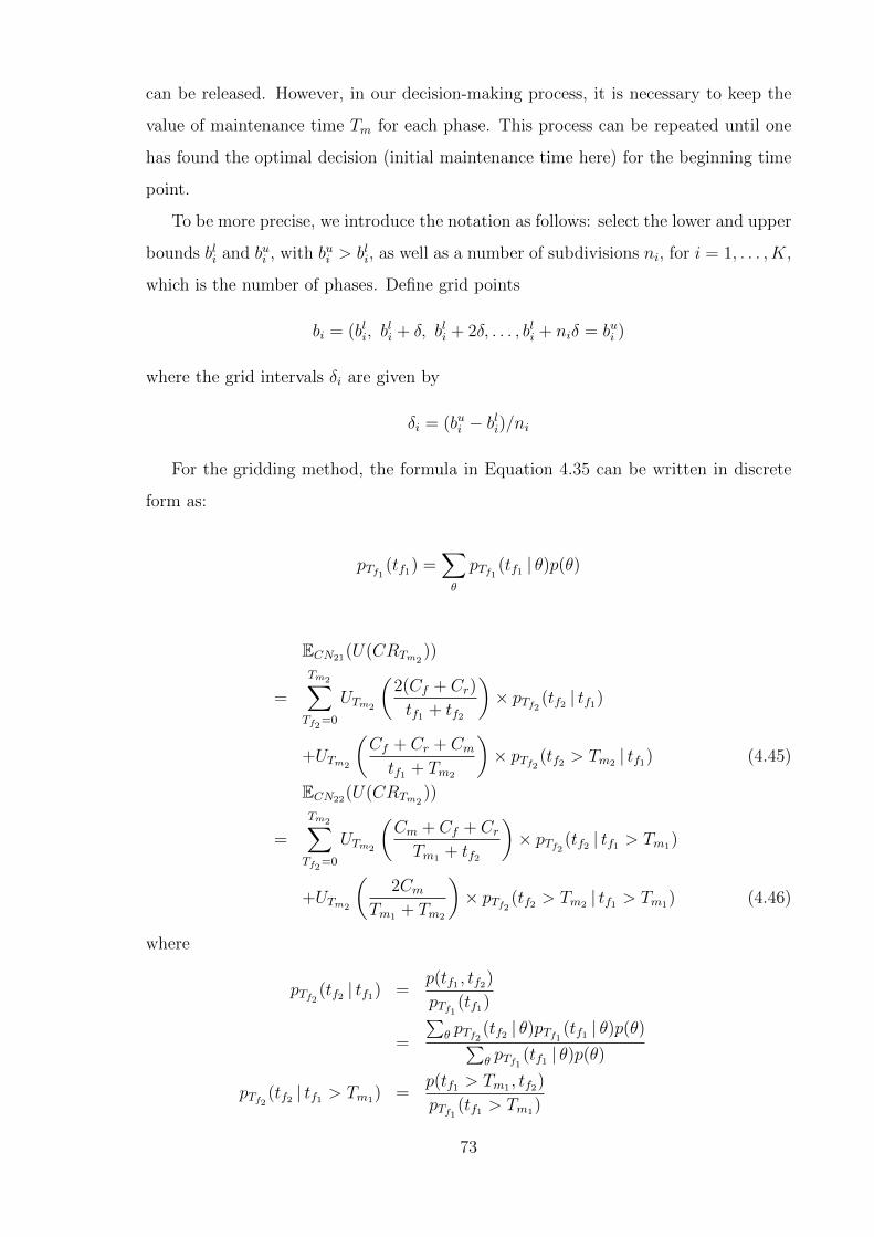
can be released. However, in our decision-making process, it is necessary to keep the
value of maintenance time Tm for each phase. This process can be repeated until one
has found the optimal decision (initial maintenance time here) for the beginning time
point.
To be more precise, we introduce the notation as follows: select the lower and upper
bounds bli and bui , with bui > bli, as well as a number of subdivisions ni, for i = 1, . . . , K,
which is the number of phases. Define grid points
bi = (bli, bli + δ, bli + 2δ, . . . , bli + niδ = bui )
where the grid intervals δi are given by
δi = (bui − bli)/ni
For the gridding method, the formula in Equation 4.35 can be written in discrete
form as:
pTf1 (tf1) =∑θ
pTf1 (tf1 | θ)p(θ)
ECN21(U(CRTm2))
=
Tm2∑Tf2=0
UTm2
(2(Cf + Cr)
tf1 + tf2
)× pTf2 (tf2 | tf1)
+UTm2
(Cf + Cr + Cmtf1 + Tm2
)× pTf2 (tf2 > Tm2 | tf1) (4.45)
ECN22(U(CRTm2))
=
Tm2∑Tf2=0
UTm2
(Cm + Cf + CrTm1 + tf2
)× pTf2 (tf2 | tf1 > Tm1)
+UTm2
(2Cm
Tm1 + Tm2
)× pTf2 (tf2 > Tm2 | tf1 > Tm1) (4.46)
where
pTf2 (tf2 | tf1) =p(tf1 , tf2)
pTf1 (tf1)
=
∑θ pTf2 (tf2 | θ)pTf1 (tf1 | θ)p(θ)∑
θ pTf1 (tf1 | θ)p(θ)
pTf2 (tf2 | tf1 > Tm1) =p(tf1 > Tm1 , tf2)
pTf1 (tf1 > Tm1)
73

=
∑θ pTf2 (tf2 | θ)pTf1 (tf1 > Tm1 | θ)p(θ)∑
θ pTf1 (tf1 > Tm1 | θ)p(θ)
By this gridding method, and for our example, we set δθ and θ is from 1 to 10; δTf as
0.1 and tf1 , tf2 is from 1 to 6.0.
0.00
0.01
0.02
0.03
0.04
2.5 5.0 7.5 10.0θ
PM
F
0.000
0.025
0.050
0.075
0 2 4 6Tf1
PM
F
Figure 4.9: Prior distribution of θ (left) and marginal distribution of Tf1 (right) by
the gridding method.
Figure 4.10 and Figure 4.11 show probabilities of Tf2 conditional on Tf1 : depending
on various tf1 from 0.1 to 6.0, it can be seen that the modes of pTf2 (tf2 | tf1) move from
left to right and reversely after reaching a certain threshold node, which demonstrates
the dynamics of conditional probabilities.
74

0.000
0.025
0.050
0.075
0.100
0 2 4 6Tf2
Density
Tf1
0.1
0.2
0.3
0.4
0.5
0.6
0.7
0.8
0.9
1
1.1
1.2
1.3
1.4
1.5
1.6
1.7
1.8
1.9
2
2.1
2.2
2.3
2.4
2.5
2.6
2.7
2.8
2.9
3
3.1
3.2
3.3
3.4
3.5
3.6
3.7
3.8
3.9
4
4.1
4.2
4.3
4.4
4.5
4.6
4.7
4.8
4.9
5
5.1
5.2
5.3
5.4
5.5
5.6
5.7
5.8
5.9
6
Figure 4.10: Probability of Tf2 conditioning on tf1 , i.e., pTf2 (tf2 | tf1 = i), where
i = 0.1, . . . , 6, by the gridding method.
75

0.000
0.025
0.050
0.075
0 2 4 6
p(tf1)p(tf2|tf1=0.1)
0.000
0.025
0.050
0.075
0 2 4 6
p(tf1)p(tf2|tf1=0.5)
0.000
0.025
0.050
0.075
0.100
0 2 4 6
p(tf1)p(tf2|tf1=1.0)
0.000
0.025
0.050
0.075
0.100
0 2 4 6
p(tf1)p(tf2|tf1=1.1)
0.000
0.025
0.050
0.075
0 2 4 6
p(tf1)p(tf2|tf1=1.5)
0.000
0.025
0.050
0.075
0 2 4 6
p(tf1)p(tf2|tf1=2.0)
0.000
0.025
0.050
0.075
0 2 4 6
p(tf1)p(tf2|tf1=2.1)
0.000
0.025
0.050
0.075
0 2 4 6
p(tf1)p(tf2|tf1=2.5)
0.000
0.025
0.050
0.075
0 2 4 6
p(tf1)p(tf2|tf1=3.0)
0.000
0.025
0.050
0.075
0 2 4 6
p(tf1)p(tf2|tf1=3.1)
0.000
0.025
0.050
0.075
0 2 4 6
p(tf1)p(tf2|tf1=3.5)
0.000
0.025
0.050
0.075
0 2 4 6
p(tf1)p(tf2|tf1=4.0)
0.000
0.025
0.050
0.075
0 2 4 6
p(tf1)p(tf2|tf1=4.1)
0.000
0.025
0.050
0.075
0 2 4 6
p(tf1)p(tf2|tf1=4.5)
0.000
0.025
0.050
0.075
0 2 4 6
p(tf1)p(tf2|tf1=5.0)
0.000
0.025
0.050
0.075
0 2 4 6
p(tf1)p(tf2|tf1=5.1)
0.000
0.025
0.050
0.075
0 2 4 6
p(tf1)p(tf2|tf1=5.5)
0.000
0.025
0.050
0.075
0 2 4 6
p(tf1)p(tf2|tf1=6.0)
Figure 4.11: Comparison of pTf1 (tf1) (red) and pTf2 (tf2 | tf1 = i) (green), where i = 0.1,
0.5, 1.0, 1.1, 1.5, 2.0, 2.1, 2.5, 3.0, 3.1, 3.5, 4.0, 4.1, 4.5, 5.0, 5.1, 5.5, 5.9.
To find the threshold node, a three-dimensional graph is plotted as Figure 4.12.
76

Figure 4.13 is the projection, in which numbers alongside the dots are Tf2 which produce
the maximum probability conditioning on corresponding Tf1 . From Figure 4.12 and
Figure 4.13, we can see that the node is at when pTf2 (tf2 = 0.9 | tf1 = 1).
0 1 2 3 4 5 60.07
00.
075
0.08
00.
085
0.09
00.
095
0.10
00.
105
0.00.2
0.40.6
0.81.0
Tf1
arg
max
p(tf
2|tf1
)
max
p(tf
2|tf1
)
Figure 4.12: 3D scatter plot for maximal probability of Tf2 conditioning on tf1 , i.e.,
max pTf2 (tf2 | tf1), with vertical lines for each point.
0.6
0.7
0.7
0.8
0.8
0.8
0.8
0.9
0.9
0.9
0.9
0.9
0.8
0.8
0.8
0.8
0.7
0.7
0.6
0.6
0.6
0.50.5
0.5 0.4 0.4 0.40.3
0.30.3
0.30.2
0.2
0.2
0.20.2
0.20.2
0.2
0.1
0.1
0.1
0.1
0.1
0.10.1
0.10.1
0.10.1
0.10.1
0.10.1
0.10.1
0.10.1
0.10.1
0.08
0.09
0.10
0 2 4 6Tf1
max
p(tf
2|tf1
)
Figure 4.13: Maximal probability of Tf2 conditioning on tf1 , i.e., max pTf2 (tf2 | tf1).
77

Figure 4.14 presents Tf2 that has maximal probability conditioning on tf1 , i.e.,
arg max pTf2 (tf2 | tf1); corresponding probabilities (rounded to 2 decimals) are shown
alongside dots that represent Tf2 which maximise the probabilities given a specific tf1 .
It can be seen that a few tf2 have the same maximal probability conditional on various
tf1 , which is because our gridding methods have limited precision. While Figure 4.15
shows the tf2 that has maximal probability and its corresponding probability value,
for example, for varying Tf1 , the maximum conditional probability is about 0.08 when
Tf2 = 4.
0.07
0.080.08
0.090.090.09 0.1
0.1 0.1 0.1 0.1 0.1
0.090.090.090.08
0.080.08
0.080.080.07
0.070.070.07
0.070.070.07
0.070.070.070.07
0.080.080.080.080.080.080.080.08
0.080.080.080.080.080.080.080.080.080.090.090.090.090.090.090.090.090.090.090.090.09
0.25
0.50
0.75
0 2 4 6Tf1
arg
max
p(tf
2|tf1
)
Figure 4.14: Tf2 that has maximal probability conditioning on tf1 , i.e.,
arg max pTf2 (tf2 | tf1); corresponding probabilities (rounded to 2 decimals) shown along-
side dots that represent Tf2 which maximise the probabilities given a specific tf1 .
78

0.1
0.2
0.3
0.4
0.5
0.6
0.7
0.8
0.9
1
1.1
1.2
1.3
1.4
1.5
1.6
1.7
1.8
1.9
2
2.1
2.22.32.42.52.62.7
2.82.933.1
3.2
3.3
3.4
3.53.63.73.83.9
4
4.1
4.2
4.3
4.4
4.54.64.74.84.955.15.25.35.45.55.65.75.85.96
0.08
0.09
0.10
0.25 0.50 0.75arg max p(tf2|tf1)
max
p(tf
2|tf1
)
Figure 4.15: Maximal probability of Tf2 and the corresponding Tf2 ; corresponding tf1
shown alongside dots.
Figure 4.16 and Figrue 4.17 illustrate the dynamics of pTf2 (tf2 | tf1 > Tm1), which
has similar property compared with that of pTf2 (tf2 | tf1).
79

0.000
0.025
0.050
0.075
0 2 4 6Tf2
Density
Tm1
0.1
0.2
0.3
0.4
0.5
0.6
0.7
0.8
0.9
1
1.1
1.2
1.3
1.4
1.5
1.6
1.7
1.8
1.9
2
2.1
2.2
2.3
2.4
2.5
2.6
2.7
2.8
2.9
3
3.1
3.2
3.3
3.4
3.5
3.6
3.7
3.8
3.9
4
4.1
4.2
4.3
4.4
4.5
4.6
4.7
4.8
4.9
5
5.1
5.2
5.3
5.4
5.5
5.6
5.7
5.8
5.9
Figure 4.16: Probability of Tf2 conditioning on tf1 > Tm1 , i.e., pTf2 (tf2 | tf1 > Tm1),
where Tm1 = 0.1, . . . , 6, by the gridding method.
80

0.000
0.025
0.050
0.075
0 2 4 6
p(tf1)p(tf2|tm1>0.1)
0.000
0.025
0.050
0.075
0 2 4 6
p(tf1)p(tf2|tm1>0.5)
0.000
0.025
0.050
0.075
0 2 4 6
p(tf1)p(tf2|tm1>1.0)
0.000
0.025
0.050
0.075
0 2 4 6
p(tf1)p(tf2|tm1>1.1)
0.000
0.025
0.050
0.075
0 2 4 6
p(tf1)p(tf2|tm1>1.5)
0.000
0.025
0.050
0.075
0 2 4 6
p(tf1)p(tf2|tm1>2.0)
0.000
0.025
0.050
0.075
0 2 4 6
p(tf1)p(tf2|tm1>2.1)
0.000
0.025
0.050
0.075
0 2 4 6
p(tf1)p(tf2|tm1>2.5)
0.000
0.025
0.050
0.075
0 2 4 6
p(tf1)p(tf2|tm1>3.0)
0.000
0.025
0.050
0.075
0 2 4 6
p(tf1)p(tf2|tm1>3.1)
0.000
0.025
0.050
0.075
0 2 4 6
p(tf1)p(tf2|tm1>3.5)
0.000
0.025
0.050
0.075
0 2 4 6
p(tf1)p(tf2|tm1>4.0)
0.000
0.025
0.050
0.075
0 2 4 6
p(tf1)p(tf2|tm1>4.1)
0.000
0.025
0.050
0.075
0 2 4 6
p(tf1)p(tf2|tm1>4.5)
0.000
0.025
0.050
0.075
0 2 4 6
p(tf1)p(tf2|tm1>5.0)
0.000
0.025
0.050
0.075
0 2 4 6
p(tf1)p(tf2|tm1>5.1)
0.000
0.025
0.050
0.075
0 2 4 6
p(tf1)p(tf2|tm1>5.5)
0.000
0.025
0.050
0.075
0 2 4 6
p(tf1)p(tf2|tm1>5.9)
Figure 4.17: Comparison of pTf1 (tf1) (red) and pTf2 (tf2 | tf1 > Tm1) (green), where
Tm1 = 0.1, 0.5, 1.0, 1.1, 1.5, 2.0, 2.1, 2.5, 3.0, 3.1, 3.5, 4.0, 4.1, 4.5, 5.0, 5.1, 5.5, 5.9.
81
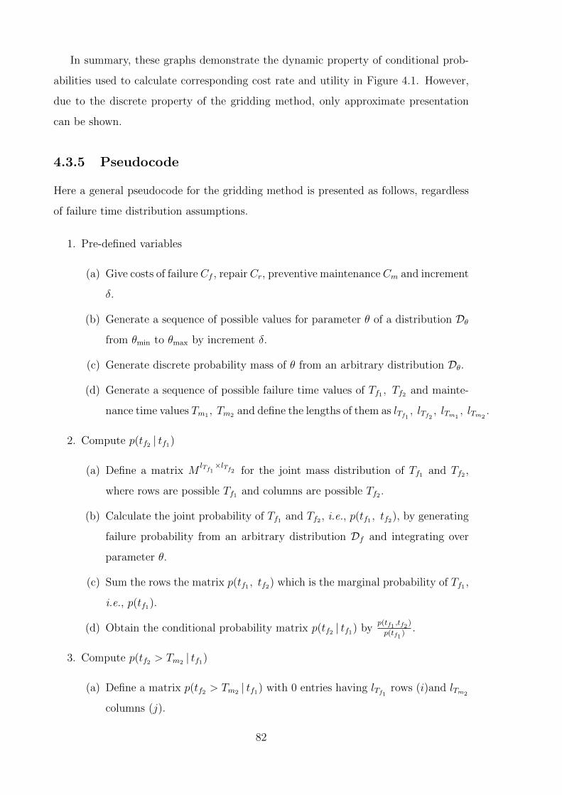
In summary, these graphs demonstrate the dynamic property of conditional prob-
abilities used to calculate corresponding cost rate and utility in Figure 4.1. However,
due to the discrete property of the gridding method, only approximate presentation
can be shown.
4.3.5 Pseudocode
Here a general pseudocode for the gridding method is presented as follows, regardless
of failure time distribution assumptions.
1. Pre-defined variables
(a) Give costs of failure Cf , repair Cr, preventive maintenance Cm and increment
δ.
(b) Generate a sequence of possible values for parameter θ of a distribution Dθfrom θmin to θmax by increment δ.
(c) Generate discrete probability mass of θ from an arbitrary distribution Dθ.
(d) Generate a sequence of possible failure time values of Tf1 , Tf2 and mainte-
nance time values Tm1 , Tm2 and define the lengths of them as lTf1 , lTf2 , lTm1, lTm2
.
2. Compute p(tf2 | tf1)
(a) Define a matrix MlTf1×lTf2 for the joint mass distribution of Tf1 and Tf2 ,
where rows are possible Tf1 and columns are possible Tf2 .
(b) Calculate the joint probability of Tf1 and Tf2 , i.e., p(tf1 , tf2), by generating
failure probability from an arbitrary distribution Df and integrating over
parameter θ.
(c) Sum the rows the matrix p(tf1 , tf2) which is the marginal probability of Tf1 ,
i.e., p(tf1).
(d) Obtain the conditional probability matrix p(tf2 | tf1) byp(tf1 ,tf2 )
p(tf1 ).
3. Compute p(tf2 > Tm2 | tf1)
(a) Define a matrix p(tf2 > Tm2 | tf1) with 0 entries having lTf1 rows (i)and lTm2
columns (j).
82

(b) For each row, update the entries by sum of the columns of p(tf2 | tf1) from
j + 1 to lTm2and obtain the joint probability of tf2 > Tm2 and tf1 , i.e.,
p(tf2 > Tm2 , tf1).
(c) Obtain the conditional probability matrix p(tf2 > Tm2 | tf1) byp(tf2>Tm2 ,tf1 )
p(tf1 ).
4. Compute p(tf2 | tf1 > Tm1)
(a) Define a vector representing p(tf1 > Tm1), of which the length is lTm1.
(b) Define a matrix for the joint probability of tf1Ttm1 and tf2 , i.e., p(tf1 >
Tm1 , tf2), of which rows are possible Tm1 and columns are possible Tf2 .
(c) For a given Tm1 , sum p(tf1) of which tf1 > Tm1 , which gives p(tf1 > Tm1).
(d) For a given Tm1 , sum p(tf1 , tf2) of which tf1 > Tm1 and corresponding tf2 ,
which gives p(tf2 , tf1 > Tm1).
(e) Obtain the conditional probability matrix p(tf2 | tf1 > Tm1) byp(tf2 , tf1>Tm1 )
p(tf1>Tm1 ).
5. Compute p(tf2 > Tm2 | tf1 > Tm1)
(a) Define a matrix p(tf2 > Tm2 | tf1) with 0 entries having (lTm1− 1) rows (i)
and lTm2columns (j).
(b) For each row, update the entries by sum of the columns of p(tf2 | tf1 > Tm1)
from j + 1 to lTm2and obtain p(tf2 > Tm2 , tf1 > Tm1).
(c) Obtain the conditional matrix p(tf2 > Tm2 | tf1 > tm1) byp(tf2>Tm2 ,tf1>Tm1 )
p(tf1>Tm1 ).
6. Calculate the expected utility of cost rate (the expected cost per unit time) at
chance node CN21 and CN22, i.e., ECN21(U(CRTm2)) and ECN22(U(CRTm2
))
(a) EUpperCN21
is a utility matrix related to tf1 and tf2 ≤ Tm2 , with lTf1 rows and
lTm2columns.
(b) ELowerCN21
is a utility matrix related to tf1 and tf2 > Tm2 , with lTf1 rows and
lTm2columns.
(c) For each row of matrix EUpperCN21
(i.e., given a possible Tf1), each entry is the
utility given a possible Tf2 , which givesCf+Crtf1+tf2
× p(tf2 | tf1).
(d) For each row of matrix ELowerCN21
(i.e., given a possible Tf1), each entry is the
utility given a possible Tm2 , which givesCf+Cr+Cmtf1+Tm2
× p(tf2 > Tm2 | tf1).
83

(e) Sum the two matrices above, i.e., EUpperCN21
and ELowerCN21
, which gives the ex-
pected utility of expected cost per unit time at chance node CN21, i.e.,
ECN21(U(CRTm2)).
(f) Apply the same process to EUpperCN22
and ELowerCN22
with different cost structures
and conditional probability matrices to obtain ECN22(U(CRTm2)).
7. Calculate the expected cost per unit time at chance node CN1, i.e., ECN1Tf1
(a) For each row of matrix ECN21(U(CRTm2)), find the maximum utility and
corresponding Tm2 , which gives the optimal Tm2 that produces maximum
utility, given a Tf1 .
(b) For each row of matrix ECN22(U(CRTm2)), find the maximum utility and
corresponding Tm2 , which gives the optimal Tm2 that produces maximum
utility, given a Tm1 .
(c) Sum the maximum utilities above pairwisely with their corresponding prob-
abilities, i.e., p(tf1) and p(tf1 > Tm1), which gives the ECN1(U(CRTm1)).
(d) Find the optimal maintenance time Tm1 that produces maximum utility
from ECN1(U(CRTm1)).
4.4 Numerical Examples
The results and related simulations are shown in this section according to previous
models proposed. Maintenance time discussed herein is “local time” (Definition 2.2).
4.4.1 PPM for Two-Phase System
For a two-phase system, we assume the failure cost as Cf = 2, repair cost as Cr = 1
and maintenance cost as Cm = 0.5, which will also apply to other examples.
To compare the results obtained through the dynamic programming framework, the
results under a myopic framework are presented as well. Within the myopic framework,
the decision maker optimises the maintenance time at the current state, but does not
explicitly use forecasting information or any direct representation of decisions in the
future. As a result the calculation is expected to be less time consuming than that
84

within the dynamic programming framework. However, its solution would not be
globally optimal since it ignores possible learning.
From Figure 4.18 we are able to see that the expected utility at chance node CN21
is decreasing due to the branch assumption of tf1 ≤ Tm1 indicating more cost induced,
while the expected utility at chance node CN22 is increasing thanks to the branch
assumption of tf1 > Tm1 . By looking for the maximum value of the expected utility at
chance node CN1, we are able to find the corresponding maintenance time, which is
the optimal maintenance time for CN1, Tm1 .
−3
−2
−1
0
0 2 4 6Tm1
Expe
cted
Util
ity ChanceNodes
CN21
CN22
CN1
Figure 4.18: Expected utilities for two-phase systems at chance nodes CN21, CN22
and CN1 under the dynamic programming method.
From Table 4.1 we can see that the optimal maintenance time Tm1 at chance node
CN1, by the dynamic programming method is 0.5, which is larger than than that by
the myopic method that is 0.3, whereas the expected utility is higher, which can be
explained as by considering all possible future decisions and previous information, and
as a result, one can reduce the cost spent on system maintenance, which in other words
improves its utility. When it comes to the second phase, if failure is not observed before
maintenance at Tm1 at local time 0.5 for the first phase, then maintenance time for
the second phase is supposed to be at local time 0.3, which can be explained as: early
maintenance decisions can be riskier so as to gain information whilst later decisions
(here the last decisions) have no or little use to gain extra information because the
85

system considered here has two phases only.
Dynamic Programming Myopic
Maintenance Time Expect Utility Maintenance Time Expected Utility
Tm1 ECRCN1 Tm1 ECRCN1
0.5 -2.56 0.3 -3.23
Tm2(Tf1 ≤ Tm1) ECRCN21 Tm2(Tf1 ≤ Tm1) ECRCN21
0.9(0.1) -8.75 0.9(0.1) -8.75
0.8(0.2) -6.86 0.8(0.2) -6.86
0.7(0.3) -5.73 0.7(0.3) -5.73
0.7(0.4) -4.95 - -
0.6(0.5) -4.37 - -
Tm2(Tf1 > Tm1) ECRCN22 Tm2(Tf1 > Tm1) ECRCN22
0.3 -1.61 0.4 -2.19
Table 4.1: Optimal corrective maintenance (CM) time and corresponding expected
cost for each chance node based on dynamic programming and myopic methods. Brack-
eted figures are failure time Tf1 with respect to T ∗m1and T ∗m2
, numbers in brackets
representing corresponding failure times.
As we can see in Figure 4.19 and Table 4.2, for very low risk aversion, in other
words, when the risk aversion parameter η → 0, exponential utility function will give
the same maintenance policy, i.e., same maintenance time by maximising expected
utility of cost rate, which tends towards minimising the expected cost per unit time or
cost rate.
86

0
1
2
3
0 2 4 6Tm1
Expe
cted
Cos
t ChanceNodes
CN21
CN22
CN1
Figure 4.19: Expected costs for two-phase systems at chance nodes CN21, CN22 and
CN1 under the dynamic programming method.
Expected Cost η → 0 Expected Utility η = 0.001
Maintenance Time Expected Cost Rate Maintenance Time Expected Utility
T ∗m1ECRCN1 T ∗m1
ETm1U(CRCN1)
0.5 2.55 0.5 -2.56
Tm2(Tf1 ≤ Tm1) ECRCN21 Tm2(Tf1 ≤ Tm1) ETm2U(CRCN21)
0.9(0.1) 8.69 0.9(0.1) -8.75
0.8(0.2) 6.83 0.8(0.2) -6.86
0.7(0.3) 5.71 0.7(0.3) -5.73
0.7(0.4) 4.93 0.7(0.4) -4.95
0.6(0.5) 4.36 0.6(0.5) -4.37
Tm2(Tf1 > Tm1) ECRCN22 T ∗m2(Tf1 > Tm1) ETm2
U(CRCN22)
0.3 1.61 0.3 -1.61
Table 4.2: Optimum Perfect Preventive Maintenance (PPM) time through different
optimisation objectives, i.e., expected cost and expected utility for each chance node
based on dynamic programming method. Bracketed figures are failure time Tf1 with
respect to Tm1 and Tm2 , numbers in brackets representing corresponding failure times.
To investigate the impact of risk aversion parameter η on the decision making about
87

the optimal maintenance time, η is increased gradually to compare the corresponding
optimal maintenance time and expected utility for chance node CN1 of the two-phase
repairable system. As it is shown in Table 4.3, with the decision maker becoming more
risk averse (i.e., larger η), one is supposed to preventively maintain the system earlier
and the expected utility decreases accordingly. Figure 4.20 shows the characteristic of
decreasing, in which the expected utility is transformed via an exponential function
exp(·) to be presented in the right graph.
Risk Aversion Parameter η Maintenance Time Expected Utility
0.001 0.5 -2.56
0.100 0.4 -3.61
0.200 0.4 -7.71
0.300 0.4 -43.49
0.400 0.4 -522.29
0.500 0.3 -7977.54
0.600 0.3 -131705.40
0.700 0.2 -2257595.00
0.800 0.2 -39617496.00
0.900 0.2 -706949065.00
Table 4.3: Optimal perfect preventive maintenance (PPM) time and corresponding
expected utility for chance node CN1 by dynamic programming conditioning on various
risk aversion parameter η of an exponential utility function.
−1e+10
−5e+09
0e+00
0.00 0.25 0.50 0.75 1.00η
Util
ity
0.00
0.02
0.04
0.06
0.08
0.00 0.25 0.50 0.75 1.00η
Exp
onen
tial U
tility
Figure 4.20: Risk aversion parameter η on utility.
According to the results obtained via the dynamic programming method, one can
88

determine the optimal maintenance times for each phase of the two phase system by
referring to Figure 4.21. For example, one determines the maintenance time for phase
1 as 0.5; if a failure occurs at time 0.2, the maintenance time for phase 2 is chosen as
0.8 at local time, i.e., 1.0(0.2 + 0.8) at global time; if no failure happens before 0.5, the
maintenance for phase 2 is decided as 0.3 at local time, i.e., 0.8(0.5 + 0.3) at global
time.
Phase 2
Phase 1 Tm1=0.5
Tm2=0.9 Tm2=0.8 Tm2=0.7 Tm2=0.7 Tm2=0.3
Tf1=0.1 Tf1=0.2 Tf1=0.3 Tf1=0.4 Tf1>=0.5
Figure 4.21: Optimal Maintenance Decision Tree for Two-Phase Systems.
Figure 4.22 shows the prior and posterior probability distributions of parameter
θ depending on the observed failure Tf1 and conducted preventive maintenance at
Tm1 = 0.5 and indicates that the posterior probability distribution of θ is more right-
skewed and has higher mode if failure occurs earlier in the first phase.
89

1 2 3 4 5 6
0.00
0.02
0.04
0.06
0.08
0.10
0.12
θ
Den
sity
p(θ)
p(θ | Tf1=0.1)
p(θ | Tf1=0.2)
p(θ | Tf1=0.3)
p(θ | Tf1=0.4)
p(θ | Tf1=0.5)
p(θ | Tf1>0.5)
Figure 4.22: Posterior probability density of θ conditioning on Tf1(≤ 0.5) and Tf1 >
0.5 compared with prior probability density of θ.
4.4.2 Simulation
A simulation is an experiment performed on a model. In this context, the experiment is
understood as varying parameters or changing the setup of the model. While the formal
modelling of systems using mathematics tries to find analytical solutions, computer-
based simulation can provide solutions to problems which are beyond the limits of
analytical approaches. Computer-based simulation uses approximation techniques (e.g.
numerical integration) to find results to problems which have no analytical solution, can
combine discrete and continuous system characteristics, or interact with the simulator.
The simulation results in this thesis coordinate with the theoretical ones obtained by
the gridding method.
By the law of large numbers, with the number N increasing in simulations, the aver-
age of the simulation results from a large number of simulations should be close to the
expected cost rate for chance node CN1, ECRCN1 , obtained by dynamic programming.
90

ECRCN1 : µCR
N Simulated Expected Cost Rate SE Variance σ2 = E [(SE− µCR)2]
1000 2.430923 1.53014e-05
5000 2.596228 3.262069e-07
20000 2.517805 6.777306e-08
50000 2.540612 3.925825e-09
100000 2.548292 4.006983e-10
Table 4.4: Two-Phase Maintenance System Simulation Results.
As can be seen in Table 4.4, the variance of the simulated expected cost rate becomes
smaller with the increasing number of simulations, N . In other words, the expected
cost rate can be approximated via a large number of simulations.
Related R code is also attached as follows.
91

1 n <- 1000 # number of theta
2 sim.theta <- rtruncnorm(n, a=1, b=Inf , mean=2, sd=1)
3
4 # generate tf1 and tf2 which follow Weibull distribution given shape parameter theta
5 tf1 <- rep(0, rep=n)
6 tf2 <- rep(0, rep=n)
7
8 k <- 1
9 while (k<=n)
10 x <- rweibull(1, shape=sim.theta[k], scale =1)
11 y <- rweibull(1, shape=sim.theta[k], scale =1)
12 # x <- rgamma(1, shape=sim.theta[k], scale =1)
13 # y <- rgamma(1, shape=sim.theta[k], scale =1)
14 if ((round(x, 1) != 0) && (round(y, 1) != 0))
15 tf1[k] <- x
16 tf2[k] <- y
17 k=k+1
18
19
20
21 # compute simulated cost for chance node CN1
22 cost.cn <- rep(0, n)
23 for (i in 1:n)
24 if (round(tf1[i], 1) <= cn1.tm1.opt)
25 if (round(tf2[i], 1) <= cn21.tm2.opt[round(tf1[i], 1)*10])
26 cost.cn[i] <- (1+ alpha)*(Cf+Cr)/
27 (round(tf1[i], 1)+round(tf2[i], 1))
28
29 else if (round(tf2[i], 1) > cn21.tm2.opt[round(tf1[i], 1)*10])
30 cost.cn[i] <- (Cf+Cr+alpha*Cm)/
31 (round(tf1[i], 1)+cn21.tm2.opt[round(tf1[i], 1)*10])
32
33
34 else if (round(tf1[i], 1) > cn1.tm1.opt)
35 if (round(tf2[i], 1) <= cn22.tm2.opt)
36 cost.cn[i] <- (Cm+alpha*(Cf+Cr))/
37 (cn1.tm1.opt+round(tf2[i], 1))
38
39 else if (round(tf2[i], 1) > cn22.tm2.opt)
40 cost.cn[i] <- (1+ alpha)*Cm/
41 (cn1.tm1.opt+cn22.tm2.opt)
42
43
44
45 # compute simulated expected cost for chance node CN1
46 mean(cost.cn)
92

Chapter 5
Sequential Maintenance Extension
Possible extensions to the sequential preventive maintenance models in Chapter 4
are discussed in this chapter as follows: imperfect preventive maintenance, preven-
tive maintenance modelling with the time value of money, modelling preventive main-
tenance in a discrete time setting as well as maintenance for parallel maintenance,
analysing the effect of failure time distribution assumptions on preventive maintenance
time and proposing an adaptive approach to solving multi-phase systems’ maintenance.
Sensitivity analysis via the parameters of sequential preventive maintenance models will
also be carried out in this chapter 1.
5.1 Imperfect Maintenance
As stated previously in Chapter 2, both perfect preventive maintenance and imperfect
preventive maintenance have been implemented and discussed. By definitions and
assumptions, after perfect preventive maintenance, the system comes to a brand new
state, of which the failure time distribution would be the same as it was initially run.
When it comes to imperfect preventive maintenance, the system would be maintained
to some level which is not as good as a brand new system, but still is able to keep the
system running on an acceptable range and level. So it is reasonable to assume that the
rate of failure time distribution would increase after imperfect preventive maintenance,
in other words, systems would deteriorate if imperfect preventive maintenance were
1Extensions to the sequential preventive maintenance models in this chapter are based on two-phase systems and results are presented with regard to maintenance time Tm1
, unless explicitly statedotherwise. Tm2
can be obtained by referring to Figure 4.21.
93

conducted, i.e., pTf2 (tf2 | tf1 > Tm1) > pTf2 (tf2 | tf1).
According to a review by Nakagawa (2012), existing imperfect preventive main-
tenance models can be categorised as: age reduction models, hazard rate reduction
models, and hybrid models of both. Via age reduction models, the virtual age of a
system would reduce to t − δ from t after imperfect preventive maintenance, i.e., the
hazard function would change from h(t) to h(t−δ), whereas the hazard function would
change from h(t) to τh(t) (τ > 1) after imperfect preventive maintenance by hazard
rate reduction modelling. And hybrid method combines them to model the hazard
rate from h(t) to τh(t − δ). A novel method by manipulating the probability matrix
pTf2 (tf2 | tf1 > Tm1) is proposed in this section.
Based on the original conditional failure probability matrix pTf2 (tf2 | tf1) by the
gridding method, the conditional failure time matrix pTf2 (tf2 | tf1 > Tm1) for perfect
preventive maintenance M is obtained by (§4.3.5, page 82). Then imperfect preventive
maintenance probability manipulation is conducted based on this matrix: for each
row, take the last arbitrary β percent values and reassign them proportionally to each
element left, a new matrixMnew is created, which can be regarded as a way of expressing
the assumption that the failure rate increases after maintenance. For simplicity, the
matrix M with entry Mij = pTf2 (Tf2 = tjf2 | tf1 > tim1) is expressed as an example as
follows
M =
0.943 0.048 0.006 0.003
0.800 0.151 0.038 0.011
0.653 0.232 0.084 0.031
0.644 0.237 0.087 0.032
where tjf2 is the jth possible value of Tf2 and tim1
is the ith possible value of Tm1 ; and
the sum of each row is 1.
Now, for each row, the last entries 0.003, 0.011, 0.031, 0.032 are replaced with 0 and
added proportionally to the other entries for each row. For example, for the first row,
0.943 + 0.003 × 0.9430.943+0.048+0.006
, 0.048 + 0.003 × 0.0480.943+0.048+0.006
and 0.173 + 0.003 ×
94

0.0060.943+0.048+0.006
, which becomes the first row of matrix Mnew,
Mnew =
0.9458 0.0481 0.0060 0.0000
0.8089 0.1527 0.0384 0.0000
0.6739 0.2394 0.0867 0.0000
0.6653 0.2448 0.0899 0.0000
and the sum of each row for matrix Mnew is still 1.
Generally, by manipulating the conditional probability matrix M pTf2 (tf2 | tf1 >
Tm1), one can take the last β amount of probability values for each row of M and real-
locate them to other entries of M for each row proportionally according to their original
values in M . This can be regarded as an alternative method to deal with conditional
probability in imperfect preventive maintenance. We can see from Figure 5.1 that the
system is more likely to fail in the second phase if imperfect preventive maintenance is
carried out than that under perfect preventive maintenance policy because the system
is not as good as new that can only be achieved by perferct preventive maintenance.
0.000
0.025
0.050
0.075
0.100
0 2 4 6Failure Time
Den
sity
p(tf1)
p(tf2|tf1>Tm1=0.5)(PPM)
p(tf2|tf1>Tm1=0.5)(IPM)
Figure 5.1: Comparison of probabilities of Tf2 conditioning on optimal Tm1 obtained
through PPM and IPM.
95

As we can see in Figure 5.2, through the manipulation of the conditional proba-
bilities, the system is more likely to fail early at the second phase if it is imperfectly
preventively maintained at Tm1 as 0.5.
0.000
0.025
0.050
0.075
0.100
0 2 4 6Failure Time
Den
sity
p(tf1)
p(tf2|tf1=0.1)
p(tf2|tf1=0.2)
p(tf2|tf1=0.3)
p(tf2|tf1=0.4)
p(tf2|tf1>Tm1=0.5)
Figure 5.2: Comparison of probabilities of Tf2 conditioning on observed Tf1 and
implemented imperfect preventive maintenance at Tm1 .
Table 5.1 presents the comparison of optimal maintenance time by dynamic pro-
gramming and myopic methods through imperfect preventive maintenance modelling
via various preventive maintenance power β. Imperfect preventive maintenance at
power β = 0 is equivalent to perfect preventive maintenance. From Table 5.1, we
can see that expected cost rates increase with respect to the increasing PM power β
because the system is more likely to fail under imperfect preventive maintenance com-
pared with perfect preventive maintenance. It may be generally concluded that under
the imperfect preventive maintenance modelling policy systems tend to be maintained
later (Tm1 = 0.6 when β = 55 vs Tm1 = 0.5 when β = 0) while expected cost per
unit time is increasing due to the system having the high possibility to fail early and
being less reliable. More interesting is that one is supposed to maintain systems even
96

later because once maintained the system is less reliable under the imperfect preventive
maintenance policy. For example, the expected cost rate increases 11.65% under the
imperfect preventive maintenance policy with PM power β = 55 compared with its
counterpart under the perfect preventive maintenance policy which is when β = 0.
Dynamic Programming Myopic
PM Power Chance Maintenance Expected Maintenance Expected
β Node Time Cost Rate Time Cost Rate
0CN1 0.5 2.55 0.4 3.21
CN22 0.3 1.61 0.3 1.86
10CN1 0.5 2.57 0.4 3.21
CN22 0.3 1.64 0.3 1.88
20CN1 0.5 2.57 0.4 3.21
CN22 0.3 1.64 0.3 1.88
30CN1 0.5 2.57 0.4 3.21
CN22 0.3 1.64 0.3 1.88
40CN1 0.5 2.58 0.4 3.21
CN22 0.3 1.64 0.3 1.89
50CN1 0.5 2.67 0.4 3.21
CN22 0.2 1.77 0.3 2.07
55CN1 0.6 2.85 0.4 3.21
CN22 0.3 1.78 0.3 2.49
Table 5.1: Optimal Imperfect Preventive Maintenance (IPM) time and corresponding
expected cost for chance nodes CN1 and CN22 conditioning on various PM power
parameter β based on dynamic programming and myopic methods.
Because the gridding method used in this study is an approximate optimisation
approach and it is more computationally expensive to apply this method when having
smaller gridding intervals, the optimal maintenance times presented in Table 5.1 are
almost identical. However, one can expect different optimal maintenance times when
the precision of grids increases.
97

5.2 Time Value of Money
In finance, the net present value (NPV) is defined as the sum of the present values of
incoming and outgoing cash flows over a period of time. According to this idea, we can
consider the payoff and cost as incoming and outgoing cash flows of the maintenance
system, respectively; in other words, a payoff or cost now is more valuable than an
identical payoff or cost in the future, which is because of a discount factor.
Discounting of future costs has been widely used in finance, where net present
value (NPV) is used as criterion for assessing alternative policies. In our maintenance
problem, if a cost induced by a maintenance policy can be delayed for a time δt, this
part of money from the cost budget can be invested for that period of time and earn
corresponding interest with rate r or one does need not to borrow that amount of
money for a period δt with rate r 2. This time value of money effect can be modelled
through discounting costs induced by a particular maintenance at time δt ahead by a
discounting factor exp(−rδt) which is the continuous compounding of interest. So we
can re-define the cost rate function as
CR(t) =f(cost to time t)
t
=
∑i exp(−rti)costi
t(5.1)
where ti is the time at which cost i occurs, r is the inflation rate or factor for costs
and t is the system performing time. Here it is assumed that it becomes less expensive
to be maintained or fail in the future and the utility function meets the requirement
of risk aversion in this case. In other words, one can replace the previous cost Ci (i is
the phase number) in Chapter 4 by exp(−rti)Ci, where ti is the local time that cost
Ci happens at.
In the maintenance decision making problem, by implementing a discount factor in
utility modelling, the maintenance would be able to depict the reality more accurately
in terms of taking time effect into the maintenance modelling procedure.
Given the time effect parameter r varying between 0 and 1, the time factor’s effect
on systems’ perfect preventive maintenance optimisation is explored.
2r is equivalent to the rate of return in finance.
98

Time Effect Parameter r Maintenance Time Expected Cost Rate Cost
r = 1.0 0.5 2.55 -
r = 0.9 0.5 2.43 4.96%
r = 0.8 0.4 2.29 5.55%
r = 0.7 0.4 2.15 6.36%
r = 0.6 0.4 2.00 6.89%
r = 0.5 0.4 1.85 7.50%
r = 0.4 0.3 1.69 8.53%
r = 0.3 0.3 1.51 10.71%
r = 0.2 0.3 1.31 13.01%
r = 0.1 0.2 1.07 18.25%
Table 5.2: Optimal Perfect Preventive Maintenance (PPM) time and corresponding
expected cost rate for chance node CN1 conditioning on various time effect parameter r
based on dynamic programming. indicates the cost rate comparison to its previous
one.
From Table 5.2 we are able to conclude generally that with the time effect more
dominating (r → 0), systems tend to be maintained earlier because it would be much
more expensive to conduct maintenance in the future, which meets our expectation; we
may also notice that the expected cost rate decreases significantly with maintenance
actions being conducted earlier. For example, when r changes from 0.9 to 0.8, main-
tenance time would be scheduled 0.1 time units in advance and the expected cost rate
would be decreased by 5.55%; and if r changes from 0.2 to 0.1, although the mainte-
nance time would be also scheduled 0.1 time units earlier, the expected cost rate would
be decreased more significantly by 18.25%. These results imply the crucial role that
the time value of money effect plays in the maintenance modelling.
Models and results presented in this section suggest that the consideration of NPV
is crucial for preventive maintenance optimisation problem in practice, which is be-
cause money is usually borrowed from banks to carry out maintenance in practical
circumstances. Therefore, a NPV could be achieved by deferring the maintenance cost
to the future, which should be taken into account in the maintenance optimisation
process.
99

5.3 Maintenance in Discrete Time
In the survival analysis of repairable systems’ maintenance, the time to failure is not
always observed in a continuous time setting. For instance, in practice tyres of fighter
aircraft are preventively replaced after about 4 ∼ 14 flights (Nakagawa, 2012). In some
situations, the lifetimes of a system are recorded depending on the number of cycles
that it is working, so there is not a calendar or clock involved, e.g., the failure time
data of a toy manufacturing system may be collected each manufacturing cycle. In
other cases, its lifetimes are not defined at the exact clock time but are statistically ob-
served monthly, seasonly, or yearly, for example. Thus it is interesting and worthwhile
considering system maintenance in a discrete time setting.
Consider the time over an indefinitely long cycle n (n = 1, 2, . . .) that a single unit
should be operating. A unit is replaced at cycle N (N = 1, 2, . . .) after its installation
or at failure, whichever occurs first. Let Pn∞n=1 denote the discrete failure distribution
that a unit fails at cycle n. Cost (Cf + Cr) is incurred for the system that is replaced
and cost Cm(< Cf + Cr) is incurred for the non-failed system that is preventively
maintained. Then, the expected cost rate for a one phase system is given by
C(TNm ) =(Cf + Cr)
∑TNmj=1 Pj + Cm
∑∞j=TNm+1 Pj∑TNm
j=1
∑∞i=j Pi
(TNm = 1, 2, . . .) (5.2)
Let hn ≡ Pn∑∞j=n Pj (n = 1, 2, . . .) be the hazard rate of the discrete Weibull distri-
bution and µ be the mean discrete failure time, i.e., µ =∑∞
=1 nPn < ∞. Then, the
Bayesian dynamic programming method in the continuous time process in chapter 4
can be applied to modelling the optimal preventive maintenance if the failure time is
assumed to be discrete.
Assume the failure time of a system follows a discrete Weibull distribution (Nak-
agawa and Osaki, 1975). Khalique (1989) discussed the statistical properties of a few
discrete failure time distributions. Formally, Tf ∼ Discrete Weibull(p, θ) indicates that
the random failure time Tf has a discrete Weibull distribution with real parameter
p (0 < p < 1), and shape parameter θ. Its probability mass function is
PTf (tf ) = (1− p)(tf )θ − (1− p)(tf+1)θ , tf = 0, 1, 2, . . . (5.3)
The probability mass function for three different real parameter settings (p =
0.01, 0.05, 0.1, 0.5, θ = 2) is illustrated below.
100

2 4 6 8 10 12t f
0.02
0.04
0.06
0.08
PMF
2 4 6 8 10 12t f
0.05
0.10
0.15
PMF
2 4 6 8 10 12t f
0.05
0.10
0.15
0.20
0.25
PMF
2 4 6 8 10 12t f
0.02
0.04
0.06
0.08
0.10
0.12
0.14
PMF
Figure 5.3: Discrete Weibull Probability Mass Functions (top-left: p = 0.01, θ = 2;
top-right: p = 0.1, θ = 2; bottom-left: p = 0.5, θ = 2; bottom-right: p = 0.9, θ = 2).
From Figure 5.3, we can see that discrete Weibull failures are more likely to happen
for the system if p is smaller.
The cumulative distribution on the support of Tf is
P(Tf ) = P(Tf ≤ tf ) = 1− (1− p)(tf+1)θ , tf = 0, 1, 2, . . . (5.4)
then the survival function is
S(tf ) = P(Tf > tf ) = (1− p)(tf )θ , tf = 0, 1, 2, . . . . (5.5)
The hazard function for discrete Weibull failure time is
h(tf ) =P(tf )
S(tf )= 1− (1− p)(tf+1)θ−(tf )θ , (5.6)
the first derivative of h(tf ) with respect to tf is
∂h(tf )
∂tf= −(1− p)−(tf )θ+(1+tf )θ
(−θ(tf )−1+θ + θ(1 + tf )
−1+θ)
log(1− p). (5.7)
It is obvious to see that (5.7) > 0 if and only if when θ > 1, which represents an
increasing hazard function.
101

We can apply the dynamic programming method to a two phase system following
a discrete Weibull failure time distribution with the same assumptions concerning the
other parameters in Chapter 4. Corresponding results are shown in Table 5.3.
Parameter p Maintenance Time Expected Cost Rate
0.01 1 0.52
0.05 1 0.63
0.09 1 0.73
0.13 1 0.83
0.17 1 0.93
0.21 1 1.03
0.25 1 1.13
0.29 1 1.23
0.33 1 1.33
0.37 1 1.43
0.41 1 1.53
0.45 1 1.63
0.49 1 1.73
Table 5.3: Optimal perfect preventive maintenance (PPM) time and corresponding
expected cost for chance node CN1 by dynamic programming conditioning on various
parameter p of a discrete Weibull failure distribution.
As we can see in Table 5.3, with the parameter p increasing, which means the
system is less likely to fail following a discrete Weibull distribution, the expected cost
rate is also increasing despite having the same maintenance time of 1 for all cases. This
means that under the same maintenance time schedule, one can reduce the expected
cost rate significantly if the system is more likely to have a discrete Weibull failure
time. Maintenance time for the second phase can be achieved via the same procedure
proposed in Chapter 4.
This section is an elementary exploration to discrete failure probability distribution.
Hence, one can consider other discrete distributions in practice.
102

5.4 Maintenance for Parallel Systems
Systems studied so far have only one unit. Now let us consider a parallel redundant
system that consists of N(N ≥ 2) identical units and the system fails when all its units
fail. Assume each unit has a failure distribution F (t) with finite mean µ.
Suppose that a one phase system is replaced at system failure or at planned time
T (0 < T <∞), whichever occurs first. Then, we have the expected cost per unit time
for a one phase system as
C(Tm;N) =
∫ Tm
0
Cf + Crt
dFN(t) +
∫ ∞Tm
CmtdFN(t) (5.8)
=
∫ Tm
0
Cf + Cr
Tf× fN(tf ) dtf +
CmTm× fN(tf > tm) (5.9)
where Cf +Cr is the cost of replacement (failure cost and repair cost) at system failure,
Cm is the cost of perfect preventive maintenance at scheduled maintenance time Tm
with Cm < Cf + Cr.
For example, one is supposed to determine the optimal preventive maintenance
time for a two unit parallel redundant system with two phases, of which two units
are identical and follow a Weibull probability distribution with the shape parameter θ
from a normal distribution truncated at 1 with mean 2 and standard deviation 1 and
scale parameter 1, which are same assumptions presented for two-phase maintenance
models in Chapter 4. The decision tree is the same as in Figure 4.1 (page 56).
Based on the gridding method, the expected cost rates for chance nodes CN21 and
CN22 are expressed as
ECN21(CRTm2;N)
=
Tm2∑Tf2=0
(2(Cf + Cr)
tf1 + tf2
)×(pTf2 (tf2 | tf1)
)N+
(Cf + Cr + Cmtf1 + Tm2
)×(pTf2 (tf2 > Tm2 | tf1)
)N, (5.10)
ECN22(CRTm2;N)
=
Tm2∑Tf2=0
(Cm + Cf + CrTm1 + tf2
)×(pTf2 (tf2 | tf1 > Tm1)
)N+
(2Cm
Tm1 + Tm2
)×(pTf2 (tf2 > Tm2 | tf1 > Tm1)
)N, (5.11)
where N is the number of parallel units of systems.
103

As it can be seen (5.10) and (5.11), the conditional probability matrices for the two
unit system are transformed via component wise matrix multiplication. Thus, one can
apply the dynamic programming method to solving the optimal preventive maintenance
problem for two unit (and even multi-unit simply via matrix multiplication) redundant
parallel systems.
One-unit System N = 1 Parallel System N = 2
Maintenance Time Expected Cost Rate Maintenance Time Expected Cost Rate
Tm1 ECRCN1 Tm1 ECRCN1
0.5 2.55 0.5 0.57
Tm2(Tf1 ≤ Tm1) ECRCN21 Tm2(Tf1 ≤ Tm1) ECRCN21
0.9(0.1) 8.69 0.8(0.1) 17.64
0.8(0.2) 6.83 0.8(0.2) 10.32
0.7(0.3) 5.71 0.7(0.3) 6.93
0.7(0.4) 4.93 0.7(0.4) 5.04
0.6(0.5) 4.36 0.6(0.5) 3.89
Tm2(Tf1 > Tm1) ECRCN22 Tm2(Tf1 > Tm1) ECRCN22
0.3 1.61 0.5 1.55
Table 5.4: Optimal perfect preventive maintenance (PPM) time and corresponding
expected cost rate for each chance node by dynamic programming for one-unit systems
and two-unit redundant parallel systems. Bracketed figures are failure time Tf1 with
respect to Tm1 and Tm2 , numbers in brackets representing corresponding failure times.
Table 5.4 shows that the expected cost per unit time for the two unit redundant
parallel system is 0.57, which is 77.85% cheaper than that for the one unit system
(2.55). Hence, one could consider a two unit redundant system if its implementing
cost rate is less than 1.96. In other words, one can take the expected cost of 1.96 as a
cut-off to determine if a parallel redundant system should be implemented in this case.
104

5.5 PPM under failure time distribution assump-
tions
Here we simply compare the failure distribution assumption’s effect on system perfect
preventive maintenance optimisation.
For example, we assume the system failure time follows Weibull and gamma dis-
tribution, respectively. These two distributions have the same shape parameter θ
(denoted as θW and θG, respectively) that has a normal distribution prior with mean
2 and standard deviation 1 truncated at 1. For a legitimate comparison, it is assumed
that the failure times TWf and TGf from two distributions have the same expectation.
Formally,
E(TWf ) = E(TGf ),
κWΓ
(1 +
1
θW
)= κGθG,
E(κWΓ
(1 +
1
θW
))= E (κGθG) ,
κWE(
Γ
(1 +
1
θW
))= κGE (θG) ,
κW = κGE (θG)
E(
Γ(
1 + 1θW
)) ,where κW and κG are the scale parameters for Weibull and gamma distributions, re-
spectively.
κW is obtained through the following steps:
1. E(θG) = 2 + φ(1)Φ(1)
= 2.2876 ((4.33), page 66);
2. Generate a large number of N random number for θW , denoted as (θsW )i, i =
1, · · · , N , from a normal distribution truncated at 1 with mean 2 and standard
deviation 1 (κG = 1), which is the same distribution of θG;
3. Apply gamma function Γ(·) to each(
1 + 1(θsW )i
), i = 1, · · · , N ;
4. Compute the mean of Γ(
1 + 1(θsW )i
), i = 1, · · · , N , which is 0.8993309 and re-
places E(
Γ(
1 + 1θW
));
5. κW is obtained as 2.543669.
105

Then we are able to apply our gridding method to obtain marginal probability of
failure time Tf from Weibull distribution with shape parameter θW and scale parameter
κW = 2.543669 and gamma distribution with shape parameter θG and scale parameter
κG = 1. As they are shown in Figure 5.4, systems under gamma distribution assump-
tion are more likely to fail earlier than that under Weibull distribution assumption, on
the condition of same expected failure time for the two distributions.
0.00
0.01
0.02
0.03
0 2 4 6Failure Time
Den
sity
Weibullgamma
Figure 5.4: Marginal Weibull and gamma probabilities of Tf1 , pW (tf1) and pG(tf1)
with same expectation, i.e., E(TWf ) = E(TGf ).
We can see the difference in effect by looking at the probability density functions
of the two distributions:
fWTf (tf |κW , θW ) =θWκW
(tfκW
)θW−1
exp
−(tfκW
)θW
∝ (tf )θW−1 exp
−(tfκW
)θW
fGTf (tf |κG, θG) =(tf )
θG−1
(θG)κGΓ(θG)exp
− tfθG
∝ (tf )
θG−1 exp
− tfθG
106

By ignoring all the normalising constants, we can see that the probability density
function of the Weibull distribution drops off much more quickly for shape parameter
θW > 1 than the gamma distribution. In the case where θW = θG = 1, they both
reduce to the exponential distribution. More importantly, the hazard increases for the
Weibull distribution but tends to be a constant for the gamma distribution.
A comparison of maintenance time and expected cost rate obtained according to
different failure distribution assumptions are presented in Table 5.5.
Weibull failure time gamma failure time
Maintenance Time Expected Cost Rate Maintenance Time Expected Cost Rate
Tm1 ECRCN1 Tm1 ECRCN1
1.2 1.00 1.0 1.66
Tm2(Tf1 ≤ Tm1) ECRCN21 Tm2(Tf1 ≤ Tm1) ECRCN21
2.3(0.1) 4.86 1.7(0.1) 7.58
2.2(0.2) 3.97 1.7(0.2) 5.83
2.1(0.3) 3.44 1.7(0.3) 4.85
2.0(0.4) 3.07 1.7(0.4) 4.19
2.0(0.5) 2.78 1.7(0.5) 3.71
1.9(0.6) 2.56 1.6(0.6) 3.34
1.8(0.7) 2.37 1.6(0.7) 3.04
1.8(0.8) 2.22 1.6(0.8) 2.80
1.8(0.9) 2.08 1.5(0.9) 2.59
1.7(1.0) 1.97 1.5(1.0) 2.42
1.7(1.1) 1.86 - -
1.6(1.2) 1.77 - -
Tm2(Tf1 > Tm1) ECRCN22 Tm2(Tf1 > Tm1) ECRCN22
0.8 0.65 0.5 0.86
Table 5.5: Optimal Perfect Preventive Maintenance (PPM) time and corresponding
expected cost rate for each chance node by dynamic programming based on Weibull and
gamma failure time assumptions. Bracketed figures are failure time Tf1 with respect
to Tm1 and Tm2 , numbers in brackets representing corresponding failure times.
From Table 5.5 we can conclude that systems with gamma failure time distribution
107

tend to be preventively maintained earlier (the maintenance time Tm1 = 1 under gamma
failure time assumption and Tm1 = 1.2 under Weibull failure time assumption) and
about 66.24% more expensive (systems under gamma failure time assumption would
induce higher expected cost rate (1.66) than that under Weibull failure time assumption
(1.00)). In this sense, it is essential to have appropriate failure time assumptions about
the systems studied in practice because failure time assumptions could result in different
maintenance policies.
5.6 Hybrid Myopic-Dynamic Programming
Maintenance modelling and optimisation for two-phase systems have been studied so
far. In practice, however, one may be faced with more complex systems with multi-
phases. Due to the problem of the “curse of dimensionality”, the model becomes much
more complicated and the computation time increases dramatically when modelling
systems with even more phases and the number of conditional probabilities is 2n,
where n is the number of phases for a system. To partially solve this problem, a hybrid
myopic-dynamic programming method is proposed for multi-phase systems.
Consider a three-phase system with the same setting and assumptions as the two-
phase system in §4.1. A decision tree concerning the optimal maintenance times for
this system is shown in Figure 5.5. A decision maker has to determine the optimal
maintenance times Tm1 , Tm2 and Tm3 for each phase before the system starts working.
The hybrid myopic-dynamic programming (H-M-DP) can be briefly explained as
follows. First, we apply the results in the form of the optimal maintenance times from
the two-phase systems to the first two phases of the three-phase systems; in other
words, we solve part DP-1 in Figure 5.5 using the dynamic programming method.
Second, conditioning on the optimal Tm1 we obtained previously, we solve part DP-2
in Figure 5.5 also by treating the posterior of related parameters (in this case, the
posterior of θ) as a new prior and implementing dynamic programming as a function
of Tf1 .
108

𝑇𝑚3
𝑇𝑚3
𝑇𝑚3
𝑇𝑚3
𝐶31
𝐶32
𝐶33
𝐶34
𝐶21
𝐶22
𝑇𝑚2
𝑇𝑚2
𝐶1 𝑇𝑚1
3(𝐶𝑟 + 𝐶𝑓)
𝑇𝑓1 + 𝑇𝑓2 + 𝑇𝑓3
2 𝐶𝑟 + 𝐶𝑓 + 𝐶𝑚
𝑇𝑓1 + 𝑇𝑓2 + 𝑇𝑚3
2 𝐶𝑟 + 𝐶𝑓 + 𝐶𝑚
𝑇𝑓1 + 𝑇𝑚2+ 𝑇𝑓3
2 𝐶𝑟 + 𝐶𝑓 + 𝐶𝑚
𝑇𝑓1 + 𝑇𝑚2+ 𝑇𝑚3
2 𝐶𝑟 + 𝐶𝑓 + 𝐶𝑚
𝑇𝑚1+ 𝑇𝑓2 + 𝑇𝑓3
𝐶𝑟 + 𝐶𝑓 + 2𝐶𝑚
𝑇𝑚1+ 𝑇𝑓2 + 𝑇𝑚3
𝐶𝑟 + 𝐶𝑓 + 2𝐶𝑚
𝑇𝑚1+ 𝑇𝑚2
+ 𝑇𝑓3
3𝐶𝑚𝑇𝑚1
+ 𝑇𝑚2+ 𝑇𝑚3
DP-1
DP-2
Figure 5.5: Decision tree for three-phase system with sequential problem with shading
indicating a range of possible outcomes for the preceding chance node; Box DP-1 and
DP-2 show the break into two period problems.
In order to apply the dynamic programming method to finding the optimal main-
tenance times for this three-phase system, one is required to have the conditional
probabilities rooting from chance nodes CN31, CN32, CN33 and CN34, which are eight
(23) conditional probabilities as below.
1. fTf3 (tf3 | tf2 , tf1)
=f(tf3 , tf2 , tf1)
f(tf2 , tf1)
=
∫θf(tf3 | tf2 , tf1 , θ)f(tf2 | tf1 , θ)f(tf1 | θ)f(θ) dθ∫
θf(tf2 | tf1 , θ)f(tf1 | θ)f(θ) dθ
=
∫θf(tf3 | θ)f(tf2 | θ)f(tf1 | θ)f(θ) dθ∫
θf(tf2 | θ)f(tf1 | θ)f(θ) dθ
2. fTf3 (tf3 > Tm3 | tf2 , tf1)
=f(tf3 > Tm3 , tf2 , tf1)
f(tf2 , tf1)
109

=
∫θf(tf3 > Tm3 | tf2 , tf1 , θ)f(tf2 | tf1 , θ)f(tf1 | θ)f(θ) dθ∫
θf(tf2 | tf1 , θ)f(tf1 | θ)f(θ) dθ
=
∫θf(tf3 > Tm3 | θ)f(tf2 | θ)f(tf1 | θ)f(θ) dθ∫
θf(tf2 | θ)f(tf1 | θ)f(θ) dθ
3. fTf3 (tf3 | tf2 > Tm2 , tf1)
=f(tf3 , tf2 > Tm2 , tf1)
f(tf2 > Tm2 , tf1)
=
∫θf(tf3 | tf2 > Tm2 , tf1 , θ)f(tf2 > Tm2 | tf1 , θ)f(tf1 | θ)f(θ) dθ∫
θf(tf2 > Tm2 | tf1 , θ)f(tf1 | θ)f(θ) dθ
=
∫θf(tf3 | θ)f(tf2 > Tm2 | θ)f(tf1 | θ)f(θ) dθ∫
θf(tf2 > Tm2 | θ)f(tf1 | θ)f(θ) dθ
4. fTf3 (tf3 > Tm3 | tf2 > Tm2 , tf1)
=f(tf3 > Tm3 , tf2 > Tm2 , tf1)
f(tf2 > Tm2 , tf1)
=
∫θf(tf3 > Tm3 | tf2 > Tm2 , tf1 , θ)f(tf2 > Tm2 | tf1 , θ)f(tf1 | θ)f(θ) dθ∫
θf(tf2 > Tm2 | tf1 , θ)f(tf1 | θ)f(θ) dθ
=
∫θf(tf3 > Tm3 | θ)f(tf2 > Tm2 | θ)f(tf1 | θ)f(θ) dθ∫
θf(tf2 > Tm2 | θ)f(tf1 | θ)f(θ) dθ
5. fTf3 (tf3 | tf2 , tf1 > Tm1)
=f(tf3 , tf2 , tf1 > Tm1)
f(tf2 , tf1 > Tm1)
=
∫θf(tf3 | tf2 , tf1 > Tm1 , θ)f(tf2 | tf1 > Tm1 , θ)f(tf1 > Tm1 | θ)f(θ) dθ∫
θf(tf2 | tf1 > Tm1 , θ)f(tf1 > Tm1 | θ)f(θ) dθ
=
∫θf(tf3 | θ)f(tf2 | θ)f(tf1 > Tm1 | θ)f(θ) dθ∫
θf(tf2 | θ)f(tf1 > Tm1 | θ)f(θ) dθ
6. fTf3 (tf3 > Tm3 | tf2 , tf1 > Tm1)
=f(tf3 , tf2 , tf1 > Tm1)
f(tf2 , tf1 > Tm1)
=
∫θf(tf3 > Tm3 | tf2 , tf1 > Tm1 , θ)f(tf2 | tf1 > Tm1 , θ)f(tf1 > Tm1 | θ)f(θ) dθ∫
θf(tf2 | tf1 > Tm1 , θ)f(tf1 > Tm1 | θ)f(θ) dθ
=
∫θf(tf3 > Tm3 | θ)f(tf2 | θ)f(tf1 > Tm1 | θ)f(θ) dθ∫
θf(tf2 | θ)f(tf1 > Tm1 | θ)f(θ) dθ
7. fTf3 (tf3 | tf2 > Tm2 , tf1 > Tm1)
=f(tf3 , tf2 > Tm2 , tf1 > Tm1)
f(tf2 > Tm2 , tf1 > Tm1)
=
∫θf(tf3 | tf2 > Tm2 , tf1 > Tm1 , θ)f(tf2 > Tm2 | tf1 > Tm1 , θ)f(tf1 > Tm1 | θ)f(θ) dθ∫
θf(tf2 > Tm2 | tf1 > Tm1 , θ)f(tf1 > Tm1 | θ)f(θ) dθ
=
∫θf(tf3 | θ)f(tf2 > Tm2 | θ)f(tf1 > Tm1 | θ)f(θ) dθ∫
θf(tf2 > Tm2 | θ)f(tf1 > Tm1 | θ)f(θ) dθ
8. fTf3 (tf3 > Tm3 | tf2 > Tm2 , tf1 > Tm1)
110

=f(tf3 > Tm3 , tf2 > Tm2 , tf1 > Tm1)
f(tf2 > Tm2 , tf1 > Tm1)
=
∫θf(tf3 > Tm3 | tf2 > Tm2 , tf1 > Tm1 , θ)f(tf2 > Tm2 | tf1 > Tm1 , θ)f(tf1 > Tm1 | θ)f(θ) dθ∫
θf(tf2 > Tm2 | tf1 > Tm1 , θ)f(tf1 > Tm1 | θ)f(θ) dθ
=
∫θf(tf3 >m3 | θ)f(tf2 > Tm2 | θ)f(tf1 > Tm1 | θ)f(θ) dθ∫
θf(tf2 > Tm2 | θ)f(tf1 > Tm1 | θ)f(θ) dθ
The conditional probabilities above are with regard to Tf3 , which are conditioning
on two joint probabilities, e.g., the calculation for pTf3 (tf3 | tf2 , tf1). This complex form
adds a challenge to computing. As a result, the gridding approach to solving the
dynamic programming problem requires the multi-dimensional matrix formalisation.
This combination of the myopic method and dynamic programming can be applied
to those expanded problems with multi-phase systems’ optimal maintenance determi-
nation.
In the proposed hybrid myopic-dynamic programming method, first we solve part
DP-1 by dynamic programming and get Tm1 as 0.5.
0.000
0.025
0.050
0.075
0 2 4 6Tf2
Den
sity
p(tf1)
p(tf2|tf1=0.1)
p(tf2|tf1=0.2)
p(tf2|tf1=0.3)
p(tf2|tf1=0.4)
p(tf2|tf1=0.5)
p(tf2|tf1>Tm1=0.5)
Figure 5.6: Comparison of probabilities of Tf2 conditioning on varying Tf1 and optimal
Tm1 .
111

Making use of this result, in Figure 5.6 we can see that p(tf2 | tf1 = i), i = 0.1, . . . , 0.5,
is mostly on the right and below p(tf1), which tells us that the system is more likely to
fail earlier if a system failure is observed.
Let us compare the prior and posterior distribution of parameter θ. By Bayes’
theorem, the posterior of θ can be shown as p(θ | tf1 ≤ Tm1) and p(θ | tf1 > Tm1):
p(θ) =φ(θ − 2)
Φ(1)(5.12)
p(θ | tf1 ≤ 0.5) =p(tf1 ≤ 0.5 | θ)p(θ)
p(tf1 ≤ 0.5)(5.13)
p(θ | tf1 > 0.5) =p(tf1 > 0.5 | θ)p(θ)
p(tf1 > 0.5). (5.14)
Figure 5.7 shows the prior and posterior distributions of parameter θ given the
failure time is left censored and right censored, respectively. If a failure occurs before
the scheduled maintenance though it is unknown by how much, the posterior of θ is
updated in the red line indicating a right-skewed property and a higher mode compared
to the prior.
112

1 2 3 4 5 6
0.00
0.01
0.02
0.03
0.04
0.05
0.06
θ
Den
sity
p(θ)
p(θ | Tf1<Tm1=0.5)
p(θ | Tf1>Tm1=0.5)
Figure 5.7: Posterior probability density of θ conditioning on Tf1 ≤ Tm1(0.5) and
Tf1 > Tm1(0.5) compared with prior probability density of θ.
Under the different conditions of failures happening before scheduled maintenance
Tm1 and maintenance is carried out at Tm1 , the distribution of the shape parameter of
the Weibull distribution is updated and treated as the prior distribution for the next
phase of the system.
Depending on the observed failure times Tf1 or schedule maintenance at Tm1 at the
first phase, we apply the dynamic programming method to find the optimal mainte-
nance times for chance node CN21 and CN22 by considering all the possible situations
in the third phase.
113

0
2
4
6
8
0 2 4 6Tm2 at CN21
Exp
ecte
d C
ost ChanceNodes
CN31
CN32
CN21
0
2
4
6
0 2 4 6Tm2 at CN21
Exp
ecte
d C
ost ChanceNodes
CN31
CN32
CN21
0
2
4
6
0 2 4 6Tm2 at CN21
Exp
ecte
d C
ost ChanceNodes
CN31
CN32
CN21
0
2
4
0 2 4 6Tm2 at CN21
Exp
ecte
d C
ost ChanceNodes
CN31
CN32
CN21
0
1
2
3
4
5
0 2 4 6Tm2 at CN21
Exp
ecte
d C
ost ChanceNodes
CN31
CN32
CN21
0
1
2
0 2 4 6Tm2 at CN22
Exp
ecte
d C
ost ChanceNodes
CN33
CN34
CN22
Figure 5.8: Expected cost rates at chance node CN21 conditioning on tf1 ≤ Tm1 (top-
left: tf1 = 0.1, top-right: tf1 = 0.2, middle-left: tf1 = 0.3, middle-right: tf1 = 0.4 and
bottom-left: tf1 = 0.5; and expected cost rates at chance node CN22 conditioning on
tf1 > Tm1 (bottom-right) under the H-DP-M method.
Figure 5.8 shows expected cost rates at chance node CN21 conditioning on tf1 ≤ Tm1
(top-left: tf1 = 0.1, top-right: tf1 = 0.2, middle-left: tf1 = 0.3, middle-right: tf1 = 0.4
and bottom-left: tf1 = 0.5; and expected cost rates at chance node CN22 conditioning
on tf1 > Tm1 (bottom-right) under the H-DP-M method.
The optimal maintenance times of the three phase system for chance nodes CN21
and CN22 and corresponding expected cost rates depending what have been observed
in the first phase are shown in Table 5.6.
114

H-M-DP (Three-Phase) DP (Two-Phase)
ChanceHistory
Maintenance Expected Maintenance Expected
Node Time Cost Rate Time Cost Rate
CN21(Tf1 ≤ Tm1)
Tf1 = 0.1 0.7 6.19 0.9 8.69
Tf1 = 0.2 0.7 5.64 0.8 6.83
Tf1 = 0.3 0.6 5.18 0.7 5.71
Tf1 = 0.4 0.6 4.79 0.7 4.93
Tf1 = 0.5 0.6 4.46 0.6 4.36
CN22(Tf1 > Tm1) Tm1 = 0.5 0.4 2.37 0.3 1.61
Table 5.6: Optimal Perfect Preventive Maintenance (PPM) time and corresponding
expected cost rate of chance nodes CN21 and CN22 for three-phase maintenance systems
based on Hybrid Myopic-Dynamic Programming and myopic methods.
From Table 5.6 we see that through hybrid myopic-dynamic programming the future
information about the system performance is taken into our maintenance modelling,
then the maintenance times at CN21 are earlier that in the same chance node for the
two phase system, which results in lower expected cost rate compared with dynamic
programming for the two-phase system.
According to the results obtained via the hybrid myopic-dynamic programming
method, one can determine the optimal maintenance times for each phase of the three
phase system by referring to Figure 5.9. For example, one determines the maintenance
time for phase 1 as 0.5; if a failure occurs at time 0.2, the maintenance time for phase 2
is chosen as 0.7; if no failure happens before 0.7, the maintenance for phase 3 is decided
as 0.8.
115

Phase 3
Phase 2
Phase 1
Tm1=0.5
Tm2=0.7
Tm3=1.0
Tm3=1.0
Tm3=0.9
Tm3=0.9
Tm3=0.9
Tm3=0.8
Tm3=0.8
Tm2=0.7
Tm3=1.0
Tm3=0.9
Tm3=0.9
Tm3=0.9
Tm3=0.8
Tm3=0.8
Tm3=0.8
Tm2=0.6
Tm3=0.9
Tm3=0.9
Tm3=0.9
Tm3=0.8
Tm3=0.8
Tm3=0.8
Tm2=0.6
Tm3=0.9
Tm3=0.9
Tm3=0.8
Tm3=0.8
Tm3=0.8
Tm3=0.7
Tm2=0.4 Tm3=0.3
Tf1=0.1
Tf1=0.2
Tf1=0.3
Tf1=0.4
Tf1>=0.5
Tf2=0.1
Tf2=0.2 Tf2=0.3 Tf2=0.4 Tf2=0.5 Tf2=0.6
Tf2>=0.7
Tf2=0.1
Tf2=0.1
Tf2=0.1
Tf2=0.2
Tf2=0.2
Tf2=0.2
Tf2=0.3
Tf2=0.3
Tf2=0.3
Tf2=0.4
Tf2=0.4
Tf2=0.4
Tf2=0.5
Tf2=0.5
Tf2=0.5
Tf2=0.6
Tf2>=0.7
Tf2>=0.6
Tf2>=0.6
Tf2>=0.4
Figure 5.9: Optimal Maintenance Decision Tree for Three-Phase Systems
116

5.7 Sensitivity Analysis
The impact of parameter variation on maintenance policies, i.e., sensitivity analysis,
is considered and presented in this section.
5.7.1 Gridding Increments
In Chapter 4, the gridding method was implemented to solve the optimisation problem
in sequential preventive maintenance models, and the increment parameter was set
up as 0.1 as default. This section is intended to analyse and understand the core of
the gridding method, i.e., the gridding increments’ impact on decisions concerning the
optimal preventive maintenance times and the relationships between them.
First, the optimal perfect preventive maintenance times based on two different
gridding increments, δ = 0.05, 0.1, are compared as an example.
As we can see in Table 5.7: under δ = 0.05, we preventively maintain systems
earlier (0.45 time units) compared with (0.5 time units) under δ = 0.1, thanks to
the increment intervals; the former also produces lower expected cost rate (2.52) than
that (2.55) of the latter, which is a 1.18% reduction. Depending on characteristics of
systems and avaialble budget, this could be a significant cost reduction for a particular
repairable system.
Second, the precision of the increment parameter δ is further investigated to un-
derstand the underlying impact of gridding increments. In this case, the increment
parameter δ decreases, i.e., the gridding interval becomes larger. As we can see in
Table 5.8, with the increment parameter increasing from 0.005 to 0.100, there is little
change with respect to the optimal maintenance times ranging from 0.4 to 0.5, i.e., it
does not change our optimal decisions significantly. However, we note that the expected
cost rate also increases with the increasing of increment parameter δ. It is worthwhile
noting that the expected cost rate is not strictly increasing with the increase of δ,
e.g., it decreases from 2.5479 to 2.5475 when δ increases from 0.085 to 0.090. That is
because it is sampled at different points with the change of the accuracy of discrete
approximation to a continuous distribution.
117

δ = 0.05 δ = 0.1
Maintenance Time Expected Cost Rate Maintenance Time Expected Cost Rate
Tm1 ECCN1 Tm1 ECCN1
0.45 2.52 0.5 2.55
Tm2(Tf1 ≤ Tm1) ECCN21 Tm2(Tf1 ≤ Tm1) ECCN21
1.00(0.05) 10.97 0.9(0.1) 8.69
0.90(0.10) 8.96 0.8(0.2) 6.83
0.85(0.15) 7.75 0.7(0.3) 5.71
0.80(0.20) 6.89 0.7(0.4) 4.93
0.75(0.25) 6.24 0.6(0.5) 4.36
0.75(0.30) 5.72 - -
0.70(0.35) 5.29 - -
0.70(0.40) 4.92 - -
0.65(0.45) 4.60 - -
Tm2(Tf1 > Tm1) ECCN22 Tm2(Tf1 > Tm1) ECCN22
0.3 1.70 0.3 1.61
Table 5.7: Comparison of optimal perfect preventive maintenance (PPM) time and
corresponding expected cost for each chance node based on different increment param-
eter δ. Bracketed figures are failure time Tf1 with respect to Tm1 and Tm2 , numbers in
brackets representing corresponding failure times.
118

Increment Parameter Maintenance Expected Computation Time
δ Time Cost Rate (seconds)
0.005 0.460 2.49 577.03
0.010 0.460 2.49 99.63
0.015 0.465 2.49 52.95
0.020 0.460 2.50 11.71
0.025 0.475 2.50 6.29
0.030 0.450 2.51 3.78
0.035 0.455 2.51 2.60
0.040 0.480 2.51 1.84
0.045 0.450 2.52 1.36
0.050 0.450 2.52 1.02
0.055 0.440 2.53 0.79
0.060 0.480 2.53 0.64
0.065 0.455 2.53 0.53
0.070 0.490 2.54 0.43
0.075 0.450 2.54 0.39
0.080 0.480 2.54 0.34
0.085 0.425 2.55 0.27
0.090 0.450 2.55 0.23
0.095 0.475 2.55 0.21
0.100 0.500 2.55 0.19
Table 5.8: Optimal perfect preventive maintenance (PPM) time and corresponding
expected cost for chance node CN1 conditioning on various increment parameter δ
based on dynamic programming.
Because of the impact on expected cost rates by the increment parameter δ, as we
are able to see from Table 5.8, the compiling time decreases dramatically from 577.03
to 99.63 seconds when the increment parameter δ changes from 0.005 to 0.010, and it
does not change much after δ = 0.020.
Other indices concerning optimal decisions are also considered. From the top-right
graph in Figure 5.10, we can see that the optimal maintenance time fluctuates with
119

respect to the increment parameter δ but not very significantly. And from the bottom-
left graph in Figure 5.10, the absolute expected cost rate increases with respect to the
increment parameter δ, while the relative expected cost, i.e., the expected cost rate per
compiling time unit, increases seemingly exponentially. As a result, decision makers in
practice choose an appropriate increment interval to trade off between accuracy and
the cost budget that they have.
0
200
400
600
0.025 0.050 0.075 0.100Gridding Interval
Com
pilin
g T
ime
(sec
onds
)
0.44
0.46
0.48
0.50
0.025 0.050 0.075 0.100Gridding Interval
Opt
imal
Mai
nten
ance
Tim
e
2.50
2.52
2.54
0.025 0.050 0.075 0.100Gridding Interval
Exp
ecte
d C
ost R
ate
0
5
10
0.025 0.050 0.075 0.100Gridding Interval
Exp
ecte
d C
ost R
ate
per
Com
pilin
g T
ime
Uni
t
Figure 5.10: Sensitivity analysis concerning gridding intervals: Compiling time (top-
left); Optimal Maintenance Time (top-right); Expected Cost Rate (bottom-left); Ex-
pected Cost Rate per Compiling Time Unit (bottom-right).
Gridding increments and choice of interval depend on the practical problems and
it is often a trade-off between accuracy and efficiency. For example, smaller intervals
would increase the accuracy to find the closest maintenance time to theoretical results,
however, it would add computing time. Therefore, it is a decision made via cooperation
among different stakeholders to seek the optimum design of system maintenance.
120

5.7.2 Cost Structure
The related costs induced by system performing is one of the core issues considered in
our maintenance modelling. So the impact of cost structure on corresponding systems
must also be considered.
In previous studies, the perfect preventive maintenance cost Cm is assumed to be
less than that of a failure and a repair, Cf + Cm. From Table 5.9, we increase the
perfect preventive maintenance cost Cm from 0.5 to 3 with fixed failure and repair
cost, in other words, the cost difference between failure and maintenance is shrinking.
As we can see, the maintenance time increases from 0.5 to 6 which is the maximum
range of the time assumption and the expected cost rate increases as well, which means
there is less advantage to maintain the system preventively if one has to spend a higher
cost to carry it out.
Cost Difference between Maintenance Failure and Repair Maintenance Expected
Failure & Maintenance ∆ Cost Cm Cost Cf + Cr Time Cost Rate
∆ = 2.5 0.5 3.0 0.5 2.55
∆ = 2.0 1.0 3.0 0.7 3.33
∆ = 1.5 1.5 3.0 0.9 3.76
∆ = 1.0 2.0 3.0 1.4 3.95
∆ = 0.5 2.5 3.0 5.2 3.96
∆ = 0.0 3.0 3.0 6.0 3.96
Table 5.9: Optimal perfect preventive maintenance (PPM) time and corresponding
expected cost for chance node CN1 conditioning on cost difference between failure and
maintenance based on dynamic programming.
The cost structure is much more complicated in practice. However, it is usually
one of the most appealing areas in management. Within business operations, decision
makers should have the ability to budget and control cost at a desired level. In partic-
ular, maintenance may account for a large proportion in the total budget. In practice,
the decision makers will work with the cost accountants and use statistical modelling
to build up a comprehensive costing database to budget and control the maintenance
cost depending on the complexity of systems.
121

5.7.3 Prior Sensitivity
We conduct our parameter analysis under the Bayesian framework, so in this section,
we analyse the impact of prior assumptions on the system maintenance time decision
making.
The expected value for the shape parameter of the Weibull distribution is set from
1 to 10. As we can see in Table 5.10, with the increasing of the prior expectation for
the shape parameter θ, the expected cost rate decreases significantly from 3.05 to 0.91,
but it has little impact on the decision about the optimal maintenance time, which
simply ranges from 0.5 to 0.6. That is because a larger expectation of θ indicates a
higher hazard (failure) rate: one can reduce the expected cost rate by applying a same
maintenance policy (here same maintenance time) to a system with a higher possibility
to fail.
E(θprior) Maintenance Time Expected Cost Rate
1 0.5 3.05
2 0.5 2.55
3 0.5 2.00
4 0.5 1.57
5 0.5 1.30
6 0.6 1.16
7 0.6 1.05
8 0.6 0.98
9 0.6 0.93
10 0.6 0.91
Table 5.10: Optimal perfect preventive maintenance (PPM) time and corresponding
expected cost for chance node CN1 conditioning on various prior mean of parameter θ
based on dynamic programming.
In Table 5.11, the standard deviation for the shape parameter θ does not have a
significant effect on making the optimal decision about the maintenance time, which
ranges from 0.4 to 0.6, or the expected cost rate, which ranges from 2.60 to 1.84.
122
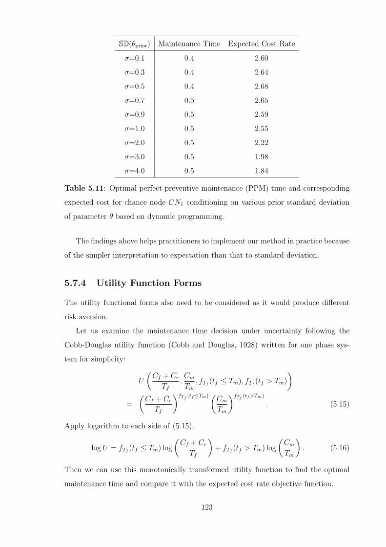
SD(θprior) Maintenance Time Expected Cost Rate
σ=0.1 0.4 2.60
σ=0.3 0.4 2.64
σ=0.5 0.4 2.68
σ=0.7 0.5 2.65
σ=0.9 0.5 2.59
σ=1.0 0.5 2.55
σ=2.0 0.5 2.22
σ=3.0 0.5 1.98
σ=4.0 0.5 1.84
Table 5.11: Optimal perfect preventive maintenance (PPM) time and corresponding
expected cost for chance node CN1 conditioning on various prior standard deviation
of parameter θ based on dynamic programming.
The findings above helps practitioners to implement our method in practice because
of the simpler interpretation to expectation than that to standard deviation.
5.7.4 Utility Function Forms
The utility functional forms also need to be considered as it would produce different
risk aversion.
Let us examine the maintenance time decision under uncertainty following the
Cobb-Douglas utility function (Cobb and Douglas, 1928) written for one phase sys-
tem for simplicity:
U
(Cf + CrTf
,CmTm
, fTf (tf ≤ Tm), fTf (tf > Tm)
)=
(Cf + CrTf
)fTf (tf≤Tm)(CmTm
)fTf (tf>Tm)
. (5.15)
Apply logarithm to each side of (5.15),
logU = fTf (tf ≤ Tm) log
(Cf + CrTf
)+ fTf (tf > Tm) log
(CmTm
). (5.16)
Then we can use this monotonically transformed utility function to find the optimal
maintenance time and compare it with the expected cost rate objective function.
123

As we can see in Table 5.12, for chance node CN1, one is suggested to maintain
the system at local time 0.5 under log utility function and expected cost rate objective
(non-log utility function).
Non-Log Utility Function Log Utility Function
Maintenance Time Expected Cost Maintenance Time Expected Cost
Tm1 ECCN1 Tm1 ECCN1
0.5 2.55 0.5 0.62
Tm2(Tf1 ≤ Tm1) ECCN21 Tm2(Tf1 ≤ Tm1) ECCN21
0.9(0.1) 8.69 1.1(0.1) 1.91
0.8(0.2) 6.83 0.9(0.2) 1.75
0.7(0.3) 5.71 0.9(0.3) 1.61
0.7(0.4) 4.93 0.8(0.4) 1.49
0.6(0.5) 4.36 0.7(0.5) 1.39
Tm2(Tf1 > Tm1) ECCN22 Tm2(Tf1 > Tm1) ECCN22
0.3 1.61 0.5 0.32
Table 5.12: Optimal perfect preventive maintenance (PPM) time and corresponding
expected cost for each chance node by dynamic programming based on non-Log and
Log utility functions. Bracketed figures are failure time Tf1 with respect to Tm1 and
Tm2 , numbers in brackets representing corresponding failure times.
However, the expected cost rate (0.62) for log utility function is much less than
that (2.55) for non-log utility function. That is because the logarithm transformation
of the expected cost rate function conveys risk aversion to the decision maker.
That is because the logarithm transformation of the expected cost rate function
presents risk aversion on the decision making. Under the non-log utility function,
because the decision maker is risk neutral, she or he is supposed to maintain the system
later compared to her or his counterpart with risk aversion, however, the maintenance
time is also 0.5, which means the system is maintained earlier than it is supposed to
be, as a result, the expected cost rate is higher than that under log transformation.
124

5.8 Parallel Computing
We have seen that the increment parameter δ is an essential element in the gridding
method to optimising the maintenance time via dynamic programming in §5.7.1. When
δ is smaller, on the one hand, it will increase the accuracy of the gridding method, which
leads one to approach the theoretically optimal maintenance time. On the other hand,
it results in a problem of being computationally expensive.
Parallel computing is a method of carrying out a large number of calculations simul-
taneously based on the principle that a complicated large problem can be independently
transformed into smaller and simpler ones. A few applications of parallel computing in
maintenance have been investigated. For example, Yang et al. (2012) build up a parallel
computing platform for multiobjective simulation optimisation of bridge maintenance
planning that can span tens of years, and also investigate the proposed framework
through a practical case, which shows the superiority to GA method.
Here the possible solutions to implement parallel computing in further research are
discussed. For example, we need to compute joint probability mass of Tf1 and Tf2 , see
Figure 5.11.
Matrix P(*2, *1)
P(*2=1, *1=1)
P(*2=1, *1=2)
P(*2=2, *1=1)
P(*2=2, *1=2)
Figure 5.11: Parallel Computing for p(tf2 , tf1)
.
If there are only two possible values of for Tf1 and Tf2 , we can calculate them
separately in four different processes independently and then combine them to form
125

the matrix for the joint probability mass.
With the development of cloud computing, decision makers could share computer
processing rescources and data to make better and coherent decisions in a comprehen-
sive and efficient manner. Although discussion of cloud computing is beyond the scope
of this thesis, it is interesting to mention that there have been some investigation on
parallel computing on maintenance. For instance, Vert et al. (2015) review models
and algorithms of a pipelineparallel computing process in intelligent scheduling. This
parallel computing process models the computing nodes’ change of resource consump-
tion, which can help decision makers to see which nodes have the highest useage in
computing. Through being implemented in a virtual cloud environment, it provides
better security and higher computing.
126

Chapter 6
Risk Aversion in Maintenance
The concept of risk aversion plays an important part in economics and finance. In
maintenance modelling, risk aversion would induce a more costly maintenance policy
but could potentially avoid huge expenditures. In this context, if one is more risk
averse, she or he would tend to maintain the system more frequently or earlier. In this
chapter, the approach proposed by Baker (2006) is used and modified to analyse the
effect of risk aversion on the variability of systems in cash flows.
6.1 Utility Functions
Baker (2006) introduces the concept of risk aversion in maintenance policies. Instead
of dealing with the expected utility per unit time, we model the expected cost per
unit time and modify the approaches to modelling in (Baker, 2006) incorporating risk
aversion.
Risk aversion is usually modelled by a concave utility function, which can be ex-
pressed as U(x), which is the utility of a sum of resources x, where U ′ > 0 and U ′′ < 0,
which are the first and second derivatives of the utility function U(x).
In this chapter, the exponential utility function is used, and defined as
U =1− exp(−ηx)
η, (6.1)
where η > 0 is the parameter measuring the risk aversion. Note that
limη→0
1− exp(−ηx)
η= x
127

and its Taylor series expansion at x = 0 is
x− η
2x2 +
η2
6x3 − η3
24x4 +
η4
120x5 − η5
720x6 +O(η6)
In other words, as η → 0, U → x, and to first order in η,
U ' x− η
2x2. (6.2)
There are a few advantages of using this utility function:
1. The exponential distribution has the memoryless property. The utility function
in (6.1) is defined with constant risk aversion, in other words, the amount of
resource that one prepares to risk is not a function of the initial resource x0; this
utility function does not depend on the resources spent on other fields either. As
a result, using of this utility function with this feature would avoid considering
one’s resources and other activities.
2. To first order in the risk aversion parameter η, all utility functions on the whole
real line will be in the form given in (6.2). Therefore, using exponential utility
function will produce more general results under lower risk aversion.
3. Most utility functions generally have more than one parameters as shown in
(§3.3.1, page 44), which would add much complexity on modelling.
As this thesis deals with costs induced by system performance, we define cost C =
−x having disutility
− U =exp(ηC)− 1
η. (6.3)
The certainty equivalent is defined as a guaranteed return that one would accept,
instead of taking a chance on a higher but uncertain and risky return. In our modelling,
we interpret it as the sum of resources that one definitely gains or loses which would
have the same expected utility as the variable cash flows via the system performance.
Therefore, if the system is performing for time T , the exponential utility function can
be expressed asexp(η · CE · T )− 1
η=
E exp(ηC)− 1
η,
where CE is the certainty equivalent per unit time, or
CE =log E exp(ηC)
ηT. (6.4)
128

6.2 Risk-averse Maintenance Modelling
We consider the preventive maintenance policy for the system modelled in chapter 4,
which would be maintained perfectly at an optimum maintenance time Tm or at failure
Tf , whichever occurs first, i.e., the length of system’s first phase is Tm or Tf , whichever
is smaller, denoted as Ti. Let the cost over the ith phase be Fi, where Fi is a random
cash flow during the phase i; in other words, Fi induced by preventive maintenance or
failure and repair, of which the cost is Cm and Cf + Cr, respectively. The certainty
equivalent per unit time for phase i is
CEi =logEexp(ηFi)
ηTi
For simplicity, the certainty equivalent per unit time for each phase is
CE =logEexp(ηF )
ηT(6.5)
by dropping the phase subscript i.
Note that the expression E exp(ηF ) in equation 6.5 is the moment generating func-
tion (m.g.f) of the random variable F with risk aversion parameter η.
When the value of the risk aversion parameter η is small, from formula 6.2, CE
reduces to
CE 'E(F ) + η
2Var(F )
T,
which shows that the cost per unit time is modified by the risk aversion parameter η
and increases with the variance of the cost induced in each phase.
Also logEexp(ηF ) is the cumulant generating function, hence
CE =
∑∞j=1 η
j−1kj/j!
T(6.6)
where kj is jth cumulant of the cost for each phase. As we can see, with the risk
aversion parameter η increasing, certainty equivalent CE also increasingly weights
towards higher cumulants, such as skewness and kurtosis.
As we model sequential preventive maintenance with unfixed maintenance time,
the length of each phase Ti is not equal. As a result, equation 6.5 becomes
exp(η · CE · T ) =N∑i=1
logE(exp(ηF ))i Pi = G(logE(exp(ηF )))
129

for a system with N phases, where Pi is the probability that i phases have occurred by
time T , therefore,
CE =log G(logE exp(ηF ))
ηT, (6.7)
where logG(·) is the cumulant generating function for the number of phases. Cox
(1962) gives the first few cumulants when expanding equation 6.7 as T →∞,
CE =
(1
k1
)logE exp(ηF )
η+
1
2!
(k2
k31
)(logE exp(ηF ))2
η
+1
3!
(3k2
2
k51
− k3
k41
)(logE exp(ηF ))3
η
+1
4!
(k4
k51
+15k3
2
k71
− 10k2k3
k61
)(logE exp(ηF ))4
η+ · · · . (6.8)
For the system considered here which is perfectly maintained at time Tm or on
failure Tf . The cost per unit time is
C(Tm) =Cf + (Cm − Cf − Cr)S(Tm)
T(6.9)
where S(·) is the survival function and Tm is optimum maintenance time obtained
in chapter 4 by dynamic programming approach. We consider the first term in the
expansion 6.8 to approximate CE.
Define I as an indicator variable, where I = 1 denotes system failure in (0, Tm] and
I = 0 denotes system has survived to time Tm with failure occurring. Therefore,
CE(Tm) =log E exp(η((Cf + Cr)I + Cm(1− I)))
ηT+ · · · , (6.10)
where T is the length of the phase.
Baker (2006) gives the expansion of the exponential as
E exp((Cf + Cr − Cm)ηI) = S(Tm) + exp(η(Cf + Cr − Cm))(1− S(Tm)),
and rearrange equation 6.10,
CE(Tm) =Cf + Cr
T+
log 1 + S(Tm)(exp(η(Cm − Cf − Cr))− 1)ηT
+ · · · . (6.11)
Then can use the equation 6.11 to analyse the relationship between risk aversion pa-
rameter η and the corresponding certainty equivalent.
130

6.3 Numerical Examples
We consider the sequential preventive maintenance model in chapter 4 where the system
is perfectly maintained preventively at Tm or at failure time Tf following a Weibull
distribution with survival function S(t) = θtθ−1, whichever occurs first, whilst the
corresponding cost is Cm and Cf + Cr, respectively. From Table 4.1 (page 86), the
optimum maintenance time Tm for phase one is 0.5 and corresponding possible failure
times Tf are 0.1, 0.2, 0.3, 0.4, 0.5.
Replace Cf as 2, Cr as 1 and Cm as 0.5 in equation 6.11,
CE(Tm = 0.5 |Tf , θ, η) =3
Tf+
log 1 + S(0.5)(exp(−2.5η)− 1)ηTf
+ · · ·
=3
Tf+
log
1 + θ0.5θ−1(exp(−2.5η)− 1)
ηTf+ · · ·(6.12)
As we can see in equation 6.12, the certainty equivalent is associated with failure time
Tf , shape parameter θ for Weibull distribution with scale parameter 1 and risk aversion
parameter η.
The shape parameter θ of the Weibull distribution is set as 2 and analysed the
relationship between the risk aversion parameter η and the certainty equivalent CE. As
we can see in Figure 6.1: first, the certainty equivalent CE increases with increasing risk
aversion; second, the certainty equivalent CE decreases with failure time increasing,
i.e., when the system is more reliable. In other words, one intends to spend less resource
if the system is more reliable.
0.05 0.10 0.15 0.20Η
20
40
60
80
100
CE
Tf1=0.5
Tf1=0.4
Tf1=0.3
Tf1=0.2
Tf1=0.1
Figure 6.1: Certainty-Equivalent with the risk-aversion parameter η under different
operating times.
131

6.4 Discussions
This chapter investigates maintenance optimisation via risk aversion from a certainty-
equivalent point of view. The aim in this section is to discuss relevant areas of interest
for further research.
• As can be seen in previous studies, utility function with very low risk aversion
provides the same maintenance policy, which tends towards minimising the av-
erage cost per unit time. Although one would be interested to know if there are
other utility functions can be applied in similar maintenance optimisation mod-
elling, it has been proved that only the linear and exponential utility functions
have properties that are reasonable to apply in practice. However, it could be
an interesting area to investigate depending on practical scenarios, e.g., nonpara-
metric utility function modelling.
• The findings that minimising the average cost per unit time is almost equivalent
to maximising the expected utility of cost rate and the certainty-equivalent cost
increases as risk aversion increases bring up the question of determing the risk
aversion parameter of the utility function. Baker (2010) suggests that one may
refer to a plot showing the relationship of certainty-equivalent cost per unit time
that is estimated from cost data and varying values of risk aversion parameter.
The certainty-equivalent cost per unit time that is not very sensitive to risk
aversion should be preferred.
132

Chapter 7
Conclusions and Future Work
7.1 Conclusions
From the utility point of view, the maintenance problems for repairable systems, includ-
ing corrective and preventive maintenance were mainly discussed. Under the framework
of Bayesian methodology, the parameters of models are random rather than fixed as
for the non-Bayesian method, while the former often suits in most of the practical
situations, the failure distribution is either unknown or contains several unknown pa-
rameters. In such case, the Bayesian approach can be quite effective to estimate these
unknown parameters by assigning prior distributions to them.
Starting from a two-phase system maintenance model, we explored the system’s
perfect preventive maintenance by dynamic programming, compared it with a myopic
method, and found the dynamic programming superior in terms of optimising mainte-
nance time. When the risk aversion parameter in the utility function is very small, our
utility-based maintenance optimisation would reduce to minimising the expected cost
per unit time.
Under different failure time distributions, we explored the effect of failure time as-
sumptions on the optimal maintenance time, and that a gamma failure time assumption
would result in later maintenance time.
Considering time effect on maintenance optimisation, we found maintenance tends
to be done earlier with the future cost becoming more expensive. Several modified
maintenance optimisation models are proposed such as modelling systems with discrete
failure distribution, parallel redundant systems.
133

By manipulating a conditional probability matrix, we explore and compare the dif-
ference between perfect preventive maintenance and imperfect preventive maintenance
and we may generally conclude that under an imperfect preventive maintenance mod-
elling framework systems tend to be maintained later because the system would enter
into a state with higher probability to fail if imperfect preventive maintenance were
conducted.
To avoid the problem of dimension increasing and to speed up computation time,
we proposed a hybrid myopic-dynamic programming method. By using the posterior
distribution for the parameter of interest, we see that the hybrid myopic-dynamic
programming maintenance time at CN21 are earlier, which results in lower expected
cost rate compared with dynamic programming for a two-phase system.
7.2 Applications
The utility-based maintenance strategies and policies proposed in this thesis are in-
tensively mathematically and theoretically modelled with a number of assumptions.
Although they are not straightforward to apply in practice, they provide new perspec-
tives on modelling preventive maintenance with modification. The prognostic mainte-
nance policies derived from historical information and system evolution require decision
makers to understand thoroughly the characteristics of the system of interest and to
anticipate all possible consequences as much as possible.
As a result, models and methodologies proposed in this thesis are more suitable for
large industrial and business purposes. The corresponding systems are supposed to be
well documented for decision makers to extract critical information and parameters for
further maintenance modelling. For example, decision makers should be able to have
access to advice from an expert if required, because expert information is essential to
justify related prior parameters to implement Bayesian dynamic programming. At the
same time, the potential future states of a system should be finite and of a relatively
small number. For instance, a personal computer’s possible states could be ‘working’,
‘sleeping’, or ‘down’, which are accountable states.
Because the methodologies in this thesis are sensitive to the number of system
states, it would not be reasonable to apply them to highly dynamic systems, such as
134

machines dealing with signal processing. Other systems that could potentially be of
interest to apply modelling methods in this thesis are an automatic manufacturing sys-
tem, a robotic process, or a computer server for the non-life essential services, in which
cases failure is neither rare or frequent, maintenance itself is not cheap or trivial, but
failure is a considerable expense, though not exorbitantly so. Hence, this approach is
not suitable to apply to maintenance of systems with very high risk aversion properties,
e.g., a nuclear power facility, an off-shore oil field, or a life support system. It is also
not worthwhile applying to trivial systems where the computational cost of performing
this analysis outweighs any savings.
In practice, there are few systems that would meet the requirements of the the-
oretical modelling, though it is the decision makers’ prerogative to adjust relevant
parameters, define overall and critical objectives, and utilise available information to
seek the pratical maintenance policies appropriate to the properties of an individual
system.
7.3 Outlook
Maintenance optimisation for repairable systems is part of maintenance theory in en-
gineering, and it also requires more attention and effort to deal with increasing issues
concerning it.
1. This research is based on utility to optimise maintenance systems. However,
it can be required to optimise several objectives simultaneously, which impose
difficulty and challenges.
2. The utility function is arbitrarily assigned in this research from a maintenance
engineering perspective. In situations where the utility function is unknown,
other theory in utility, for example, adaptive utility, can be explored.
3. Failure time distributions are in parametric form in this thesis, so it could be
interesting to explore semi-parametric and non-parametric assumptions in future
research.
4. Systems considered in this research are relatively simple, however, as the com-
plexity of systems in modern society increases, high demand to deal with the
135

maintenance on complex systems requires us to explore this field, despite the
huge mathematical and computational challenges.
5. As economies grow in modern society, there is a vast increasing demand for
resources, including human and material. Hence it is worthwhile considering
these constraints in future maintenance optimisation modelling.
136

Appendix A
Glossary
,≺,∼ Binary preference relations
θ Shape parameter of Weibull lifetime distribution
κ Scale parameter of Weibull lifetime distribution
η Risk aversion parameter
B Budget
Cf Cost induced by failure
Cm Cost induced by maintenance
Cr Cost induced by repair
CNi Chance node i
Df Arbitrary probability distribution
EU(·) Expected utility function
Ti Local time i
Tfi Failure time for phase i
Tmi Maintenance time for phase i
U(·) Utility function
Xi Global time i
137

138

Appendix B
Mathematical Proofs
B.1 Iso-elastic Utility Functions
A class called iso-elastic utility functions have the following form
U(x) =
x1−a−11−a for a > 0, a 6= 1;
log(x) the limiting case for a = 1.
These functions have the property of iso-elesticity, which means that we get the same
utility function (a positive affine transformation) if the cost is scaled by some constant
k. Formally,
For all k > 0,
U(kx) = f(k)U(x) + g(k),
for some function f(k) > 0 which is independent of x and some function g(k) which is
independent of x as well.
First consider the case when a 6= 1,
U(kx) =(kx)1−a − 1
1− a
= k1−a(x1−a − 1
1− a
)+k1−a − 1
1− a
= k1−aU(x) +k1−a − 1
1− aThe log function can be written as
U(kx) = log(kx)
= log(k) + log(x)
= U(x) + log(k)
139

B.2 Negative Exponential Utility Functions
A negative exponential utility function is of the form
U(x) = − exp −ax .
Since the first derivative U ′(x) = a exp −ax > 0 and the second derivative
U ′′(x) = −a2 exp −ax < 0, this one is also a legitimate utility function.
The class of negative exponential utility functions has an interesting property that
it is invariant under any cost transformation, i.e., for any constant k,
U(k + x) = f(k)U(x) + g(k),
for some function f(k) > 0 which is independent of x and some function g(k) which is
independent of x as well, it can be verified as below:
U(k + w) = − exp −a(k + x)
= − exp −ka exp −ax
= exp −kaU(x)
B.3 Certainty Equivalent
In general, the certainty equivalent CE for a maintenance policy whose consequence is
given by a random variable X is:
CE = U−1(E(U(X)))
U(CE) = E(U(X))
If a decision maker with utility function U has the current cost budget less than
CE, she will regard the system less reliable and tend to maintain the system earlier;
if her current cost budget is more than CE, she will think the system is more reliable
and tend to maintain the system later; and if her current cost budget is exactly CE,
she will be thinking there is no difference between maintain the system earlier or not.
Decision makers use utility functions to compare different decisions to each other.
In this sense, we can rescale a utility function via multiplying it by a positive constant
and/or adding any other positive or negative constant, which is called a positive affine
140

transformation. Two utility functions produce the same results if they are connected
via a positive affine transformation.
Suppose we have constants alpha > 0 and β and a utility function U ; another
utility function V is defined via U, α and β as:
V (x) = αU(x) + b
Since
V ′(x) = αU ′(x) > 0 because α > 0 and U ′(x) > 0
V ′′(x) = αU ′′(x) < 0 because α > 0 and U ′′(x) < 0,
V is a legitimate utility function.
If one can make a decision with consequence that is given by a random variable X,
let CE be the certainty equivalent with utility function U , then
CE = U−1(E(U(X)))
U(CE) = E(U(X))
V (CE) = αU(CE) + β
= αE(U(X)) + β
= E(V (X))
CE = V −1(E(V (X)))
So we regard the two utility functions U and V the same.
B.4 Risk Aversion
We say that two utility functions are the same if they are connected via a positive
affine transformation
V (X) = αU(X) + β
The first and second derivatives of both sides are
V ′(X) = αU ′(X)
U ′′(X) = αU ′′(X)
141

By division, we obtainV ′′(X)
V ′(X)=U ′′(X)
U ′(X)
Assume that there exists such a pair of functions U and V for which V ′′(X)V ′(X)
= U ′′(X)U ′(X)
holds and let
g(X) =V ′(X)
U ′(X)
Its first derivative
g′ = (V ′(U ′)−1)′
= V ′′(U ′)−1 + V ′(−1)(U ′)−2U ′′
=V ′′
U ′− V ′U ′′
(U ′′)2
=V ′′U ′ − V ′U ′′
(U ′′)2
=0
(U ′′)2
= 0
Since g′ = 0, g(X) = α for some constant α, then
V ′(X) = αU ′(X)
Integrals of both sides are∫V ′(X) dx =
∫αU ′(X) dx
V (X) = αU(X) + β for some constant β
Now we show that if and only if their second derivatives and first derivatives are the
same, the two utility functions can be regarded as same.
142

Appendix C
Computational Notes
The statistical computation in this thesis are written in R code (R Core Team, 2015) ,
running on a MacBook Pro (mid 2012) with an Intel Core i7 2.9 GHz CPU.
1 ## ---- myrcode1
2 # two -time period system
3
4 # pre -defined variables
5 Cf <- 2 # failure cost
6 Cr <- 1 # repair cost
7 Cm <- 0.5 # maintenace cost
8 alpha <- 1 # time effect parameter , discount rate: <=1
9
10 library(truncnorm)
11 delta <- 0.1 # increment
12 theta.poss <- seq(from=1, to=10, by=delta) # possible values of theta
13 theta.mass <- dtruncnorm(theta.poss , a=1, b=Inf , mean=2, sd=1)
14 theta.prob <- theta.mass/sum(theta.mass) # probability of theta
15
16 # possible values and lengths of tf1 , tf2 , tm1 and tm2
17 tf1.poss <- seq(from=delta , to=6, by=delta)
18 tf2.poss <- seq(from=delta , to=6, by=delta)
19 tm1.poss <- seq(from=delta , to=6, by=delta)
20 tm2.poss <- seq(from=delta , to=6, by=delta)
21 tf1.n <- length(tf1.poss)
22 tf2.n <- length(tf2.poss)
23 tm1.n <- length(tm1.poss)
24 tm2.n <- length(tm2.poss)
25
26 # compute tf2gtf1.prob: p(tf2|tf1)
27 # define a matrix for the joint mass distribution of tf1 & tf2
28 # rows are possible tf1 and columns are possible tf2
29 tf2gtf1.upper <- matrix(rep(0, tf1.n*tf2.n), nrow=tf1.n, ncol=tf2.n)
30 for (i in 1:tf1.n)
143

31 for (j in 1:tf2.n)
32 tf2gtf1.upper[i, j] <- sum(dweibull(tf1.poss[i], shape=theta.poss , scale =1)
33 *dweibull(tf2.poss[j], shape=theta.poss , scale =1)
34 *theta.prob)
35 # tf2gtf1.upper[i, j] <- sum(dgamma(tf1.poss[i], shape=theta.poss , scale =1)
36 # *dgamma(tf2.poss[j], shape=theta.poss , scale =1)
37 # *theta.prob)
38
39
40 # joint prob of tf1 and tf2: p(tf1 , tf2)
41 tf2gtf1.upper.prob <- tf2gtf1.upper/sum(tf2gtf1.upper)
42 # marginal prob of tf1: p(tf1)
43 tf2gtf1.lower.prob <- rowSums(tf2gtf1.upper.prob)
44 # conditional prob of tf2 given tf1: p(tf2|tf1)
45 tf2gtf1.prob <- exp(log(tf2gtf1.upper.prob)-log(tf2gtf1.lower.prob))
46
47 # plot tf2gtf1.prob: p(tf2|tf1)
48 # convert matrix tf2gtf1.prob to a data frame with possible tf2
49 tf2gtf1.prob.frame <- data.frame(t(tf2gtf1.prob), Tf2=tf2.poss)
50 # convert the data frame from "wide" format to "long" format
51 library(reshape2)
52 tf2gtf1.prob.long <- melt(tf2gtf1.prob.frame ,
53 id.vars="Tf2",
54 variable.name="Tf1",
55 value.name="Density")
56 levels(tf2gtf1.prob.long$Tf1) <- tf1.poss # set the variables as possible tf1
57 library(grDevices)
58 library(ggplot2)
59 ggplot(data=tf2gtf1.prob.long , # tf1 from delta to 6
60 aes(x=Tf2 , y=Density , colour=Tf1)) +
61 geom_line()
62 # ggplot(data=tf2gtf1.prob.long [1:1800 , ], # tf1 from delta to 3
63 # aes(x=Tf2 , y=Density , colour=Tf1)) +
64 # geom_line()
65 # ggplot(data=tf2gtf1.prob.long [1801:3600 , ], # tf1 from 3+delta to 6
66 # aes(x=Tf2 , y=Density , colour=Tf1)) +
67 # geom_line()
68
69
70 max.prob.tf2 <- apply(tf2gtf1.prob , 1, max)
71 max.tf2 <- delta*apply(tf2gtf1.prob , 1, which.max)
72 # create a data frame
73 # highest probability , max tf2 given tf1
74 hpmtf2gtf1 <- data.frame(tf1.poss , max.tf2 , max.prob.tf2)
75
76 # for each tf1.poss , the highest prob of tf2
77 ggplot(hpmtf2gtf1 , aes(x=tf1.poss , y=max.prob.tf2)) +
78 geom_point() +
79 geom_line() +
144

80 geom_text(aes(x=tf1.poss +0.08 , label=max.tf2), size=2, hjust =0) +
81 xlab("Tf1") + ylab("Highest probability value w.r.t Tf2")
82 # for each tf1.poss , the tf2 that has the highest prob
83 ggplot(hpmtf2gtf1 , aes(x=tf1.poss , y=max.tf2)) +
84 geom_point() +
85 geom_text(aes(y=max.tf2 +0.01 , label=round(max.prob.tf2 , 2)),
86 size=2, vjust =0) +
87 xlab("Tf1") + ylab("Tf that has the highest probability")
88 # for each tf1.poss , the tf2 that has the highest prob and its prob
89 ggplot(hpmtf2gtf1 , aes(x=max.tf2 , y=max.prob.tf2)) +
90 geom_point() +
91 geom_text(aes(x=max.tf2 +0.015 , label=tf1.poss),
92 size=2, hjust =0) +
93 xlab("Tf2 that has the highest probability given Tf1") +
94 ylab("Highest probability value w.r.t Tf2")
95 # # scatter 3d plot for tf1.poss , max.tf2 and max.prob.tf2
96 # library(scatterplot3d)
97 # scatterplot3d(tf1.poss , max.tf2 , max.prob.tf2 ,
98 # xlab="Tf1", ylab="Tf2 that has highest density given Tf1",
99 # zlab=" Density ")
100
101 # compute centf2gtf1.prob , i.e., p(tf2 >tm2|tf1)
102 centf2gtf1.prob <- matrix(rep(0, tf1.n*tm2.n), nrow=tf1.n, ncol=tm2.n)
103 for (i in 1:tf1.n)
104 for (j in 1:( tm2.n-1))
105 centf2gtf1.prob[i, j] <- sum(tf2gtf1.prob[i, (j+1):tm2.n])
106
107
108
109 # compute tf2gtm1.prob , i.e., p(tf2|tf1 >tm1)
110 # define a vector representing p(tf1 >tm1), of which the length is tm1.n
111 tf2gtm1.lower.prob <- rep(0, tm1.n)
112 # define a matrix for the joint prob of tf1 >tm1 and tf2 , i.e., p(tf1 >tm1 , tf2)
113 # rows are possible tm1 and columns are possible tf2
114 tf2gtm1.upper.prob <- matrix(rep(0, tm1.n*tf2.n), nrow=tm1.n, ncol=tf2.n)
115 for (i in 1:tm1.n)
116 tf2gtm1.lower.prob[i] <- sum(tf2gtf1.lower.prob[tf1.poss >tm1.poss[i]])
117 # tf2gtm1.lower.prob is p(tf1 >tm1)
118 # for a given tm1 , sum p(tf1) of which tf1 >tm1
119 for (j in 1:tf2.n)
120 tf2gtm1.upper.prob[i, j] <- sum(tf2gtf1.upper.prob[tf1.poss >tm1.poss[i],j])
121 # tf2gtm1.upper.prob is the joint p(tf1 >tm1 , tf2)
122 # for a given tm1 , sum p(tf1 , tf2) of which tf1 >tm1 and corresponding tf2
123
124
125 tf2gtm1.prob <- exp(log(tf2gtm1.upper.prob[-tm1.n, ])-
126 log(tf2gtm1.lower.prob[-tm1.n]))
127 # tf2gtm1.prob is P(tf2|tf1 >tm1)
128 # use [-tm1.n] to disgard the last one as it is NaN
145

129 # p(tf2|tf1 >tm1.poss[tm1.n])=0/0 which is NaN
130
131 # compute centf2gtm1 , i.e., p(tf2 >tm2|tf1 >tm1)
132 centf2gtm1.prob <- matrix(rep(0, (tm1.n-1)*tm2.n), nrow=tm1.n-1, ncol=tm2.n)
133 for (i in 1:( tm1.n-1))
134 for (j in 1:( tm2.n-1))
135 centf2gtm1.prob[i, j] <- sum(tf2gtm1.prob[i, (j+1):tm2.n])
136
137
138
139 # for preventive maintenance (PM)
140 # we assume that the failure rates incrase after PM
141 # i.e., p(tf2|tf1 >tm1) > p(tf2|tf1)
142 # for each row , the number of entries to be re-allocated
143 # prop is an integer number from 1 to ncol -1,
144 # which is the number of prob(s) taken out from each row
145 prop <- 55
146 prop.tf2gtm1.prob <- matrix(rep(0, (tm1.n-1)*tf2.n), nrow=tm1.n-1, ncol=tf2.n)
147 # for each row of tf2gtm1.prob , i.e., P(tf2|tf1 >tm1),
148 # take the sum of entries from prop+1 to ncol ,
149 # allocate it to other entries from 1 to prop
150 # depending their proportions in their own sum;
151 # replace entries from prop+1 to ncol with 0.
152 for (i in 1:( tm1.n-1))
153 prop.tf2gtm1.prob[i, ] <- c(tf2gtm1.prob[1, 1:(tf2.n-prop)]+
154 sum(tf2gtm1.prob[1, (tf2.n-prop +1):tf2.n])*
155 tf2gtm1.prob[1, 1:(tf2.n-prop)]/
156 (sum(tf2gtm1.prob[1, 1:(tf2.n-prop)])),
157 rep(0,prop))
158
159 # compute new p(tf2 >tm2|tf1 >tm1)
160 cenprop.tf2gtm1.prob <- matrix(rep(0, (tm1.n-1)*tm2.n),
161 nrow=tm1.n-1, ncol=tm2.n)
162 for (i in 1:( tm1.n-1))
163 for (j in 1:( tm2.n-1))
164 cenprop.tf2gtm1.prob[i, j] <- sum(prop.tf2gtm1.prob[i, (j+1):tm2.n])
165
166
167
168 par(mfrow=c(3,2))
169 plot(tf1.poss , tf2gtf1.lower.prob , type="l", col="black", lty=1,
170 xlab="Tf2", ylab="p(tf2|tf1 >1)")
171 lines(tf2.poss , tf2gtm1.prob[10, ], col="red", lty=2)
172 lines(tf2.poss , prop.tf2gtm1.prob[10, ], col="blue", lty=3)
173 abline(v=tf2.poss[which.max(tf2gtf1.lower.prob)], col="black", lty=1)
174 abline(v=tf2.poss[which.max(tf2gtm1.prob[10, ])], col="red", lty=2)
175 abline(v=tf2.poss[which.max(prop.tf2gtm1.prob[10, ])], col="blue", lty =3)
176
177 plot(tf1.poss , tf2gtf1.lower.prob , type="l", col="black", lty=1,
146

178 xlab="Tf2", ylab="p(tf2|tf1 >2)")
179 lines(tf2.poss , tf2gtm1.prob[20, ], col="red", lty=2)
180 lines(tf2.poss , prop.tf2gtm1.prob[20, ], col="blue", lty=3)
181 abline(v=tf2.poss[which.max(tf2gtf1.lower.prob)], col="black", lty=1)
182 abline(v=tf2.poss[which.max(tf2gtm1.prob[20, ])], col="red", lty=2)
183 abline(v=tf2.poss[which.max(prop.tf2gtm1.prob[20, ])], col="blue", lty =3)
184
185 plot(tf1.poss , tf2gtf1.lower.prob , type="l", col="black", lty=1,
186 xlab="Tf2", ylab="p(tf2|tf1 >3)")
187 lines(tf2.poss , tf2gtm1.prob[30, ], col="red", lty=2)
188 lines(tf2.poss , prop.tf2gtm1.prob[30, ], col="blue", lty=3)
189 abline(v=tf2.poss[which.max(tf2gtf1.lower.prob)], col="black", lty=1)
190 abline(v=tf2.poss[which.max(tf2gtm1.prob[30, ])], col="red", lty=2)
191 abline(v=tf2.poss[which.max(prop.tf2gtm1.prob[30, ])], col="blue", lty =3)
192
193 plot(tf1.poss , tf2gtf1.lower.prob , type="l", col="black", lty=1,
194 xlab="Tf2", ylab="p(tf2|tf1 >4)")
195 lines(tf2.poss , tf2gtm1.prob[40, ], col="red", lty=2)
196 lines(tf2.poss , prop.tf2gtm1.prob[40, ], col="blue", lty=3)
197 abline(v=tf2.poss[which.max(tf2gtf1.lower.prob)], col="black", lty=1)
198 abline(v=tf2.poss[which.max(tf2gtm1.prob[40, ])], col="red", lty=2)
199 abline(v=tf2.poss[which.max(prop.tf2gtm1.prob[40, ])], col="blue", lty =3)
200
201 plot(tf1.poss , tf2gtf1.lower.prob , type="l", col="black", lty=1,
202 xlab="Tf2", ylab="p(tf2|tf1 >5)")
203 lines(tf2.poss , tf2gtm1.prob[50, ], col="red", lty=2)
204 lines(tf2.poss , prop.tf2gtm1.prob[50, ], col="blue", lty=3)
205 abline(v=tf2.poss[which.max(tf2gtf1.lower.prob)], col="black", lty=1)
206 abline(v=tf2.poss[which.max(tf2gtm1.prob[50, ])], col="red", lty=2)
207 abline(v=tf2.poss[which.max(prop.tf2gtm1.prob[50, ])], col="blue", lty =3)
208
209 plot(tf1.poss , tf2gtf1.lower.prob , type="l", col="black", lty=1,
210 xlab="Tf2", ylab="p(tf2|tf1 >5.9)")
211 lines(tf2.poss , tf2gtm1.prob[59, ], col="red", lty=2)
212 lines(tf2.poss , prop.tf2gtm1.prob[59, ], col="blue", lty=3)
213 abline(v=tf2.poss[which.max(tf2gtf1.lower.prob)], col="black", lty=1)
214 abline(v=tf2.poss[which.max(tf2gtm1.prob[59, ])], col="red", lty=2)
215 abline(v=tf2.poss[which.max(prop.tf2gtm1.prob[59, ])], col="blue", lty =3)
216
217 # p(tf1) vs p(tf2|tf1 >tm1*=0.5)(CM) vs p(tf2|tf1 >tm1*=0.5)(PM)
218 par(mfrow=c(1,1))
219 plot(tf2.poss , prop.tf2gtm1.prob[6, ], type="l", col="blue", lty=2, lwd=2.5,
220 xlab="Tf2", ylab="p(tf2|tf1 >tm1*)")
221 lines(tf2.poss , tf2gtm1.prob[5, ], col="red", lty=2, lwd =2.5)
222 lines(tf1.poss , tf2gtf1.lower.prob , col="black", lty=1, lwd =2.5)
223 lines(tf1.poss , tf2gtf1.lower.prob)
224 legend (3.5, 0.30,
225 c("p(tf1)", "p(tf2|tf1 >tm1*=0.5) (CM)", "p(tf2|tf1 >tm1*=0.6) (PM)"),
226 lty=c(1, 2, 2),
147

227 lwd=c(2.5, 2.5, 2.5),
228 col=c(1, 2, 4))
229
230 ######
231 # dynamic programming
232
233 # calculate expectated cost per unit time at chance node CN21 and CN22 ,
234 # i.e., euc21 and euc22.
235
236 # euc21.upper is a cost matrix related to tf1 and tf2 <=tm2 ,
237 # for each row (given a possible tf1),
238 # each entry is the cost given a possible tm2;
239 # e.g., the euc21.upper[1, 2] is the average cost per unit time
240 # when tf1=tf1.poss[1], and tf2=tf2.poss[1], tf2.poss[2],
241 # where tm2=tm2.poss[2],
242 # i,e., euc21.upper[1, 2]= utility(tf1=tf1.poss[1], tf2=tf2.poss [1])+
243 # utility(tf1=tf1.poss[1], tf2=tf2.poss [2]).
244 euc21.upper <- matrix(rep(0, tf1.n*tm2.n), nrow=tf1.n, ncol=tm2.n)
245 for (i in 1:tf1.n)
246 euc21.upper[i, 1] <- (1+ alpha)*(Cf+Cr)/
247 (tf1.poss[i]+tf2.poss [1])*
248 tf2gtf1.prob[i, 1]
249 for (j in 2:tm2.n)
250 euc21.upper[i, j] <- euc21.upper[i, j-1]+
251 (1+ alpha)*(Cf+Cr)/
252 (tf1.poss[i]+tf2.poss[j])*
253 tf2gtf1.prob[i, j]
254
255
256
257 # euc21.lower is a cost matrix related to tf1 and tf2 >tm2 ,
258 # for each row (given a possible tf1),
259 # each entry is the cost given a pssoible tm2;
260 # e.g., the euc21.lower[1, 2] is the average cost per unit time
261 # when tf1=tf1.poss [1] and tm2=tm2.poss[2],
262 # i.e., euc21.lower[1, 2]= utility(tf1=tf1.poss[1], tm2=tm2.poss [2]).
263 euc21.lower <- matrix(rep(0, tf1.n*tm2.n), nrow=tf1.n, ncol=tm2.n)
264 for (i in 1:tf1.n)
265 for (j in 1:( tm2.n-1))
266 euc21.lower[i, j] <- (Cf+Cr+alpha*Cm)/
267 (tf1.poss[i]+tm2.poss[j])*
268 centf2gtf1.prob[i, j]
269
270
271 # add the two matrices above , i.e., euc21.upper+euc21.lower ,
272 # give the matrix of expected cost per unit time at chance node CN21 ,
273 # i.e., euc21 ,
274 # which is associated with given tf1 and tm2 ,
275 # e.g, euc21[1, 2] is the expected cost per unit time
148

276 # when tf1=tf1.poss [1] and tm2=tm2.poss [2].
277 euc21 <- euc21.upper+euc21.lower
278
279 # cn21.tm2 is the tm2 that minimise the cost
280 # cn21.min is the minimal cost
281 cn21.tm2 <- rep(0, tf1.n)
282 cn21.min <- rep(0, tf1.n)
283 for (i in 1:tf1.n)
284 # for a given tf1 ,
285 # the tm2 that minimise the cost and associated cost.
286 cn21.tm2[i] <- tm2.poss[which.min(euc21[i, ])]
287 cn21.min[i] <- min(euc21[i, ])
288
289
290 # euc22.upper is a cost matrix related to tm1 and tf2 <=tm2 ,
291 # for each row (given a possible tm1),
292 # each entry is the cost given a possible tm2;
293 # e.g., the euc22.upper[1, 2] is the average cost per unit time
294 # when tm1=tfm.poss[1], and tf2=tf2.poss[1], tf2.poss[2],
295 # where tm2=tm2.poss[2],
296 # i,e., euc22.upper[1, 2]= utility(tm1=tm1.poss[1], tf2=tf2.poss [1])+
297 # utility(tm1=tm1.poss[1], tf2=tf2.poss [2]).
298 euc22.upper <- matrix(rep(0, (tm1.n-1)*tm2.n), nrow=tm1.n-1, ncol=tm2.n)
299 for (i in 1:( tm1.n-1))
300 euc22.upper[i, 1] <- (Cm+alpha*(Cf+Cr))/
301 (tm1.poss[i]+tf2.poss [1])*
302 prop.tf2gtm1.prob[i, 1]
303 for (j in 2:tm2.n)
304 euc22.upper[i, j] <- euc22.upper[i, j-1]+
305 (Cm+alpha*(Cf+Cr))/(tm1.poss[i]+tf2.poss[j])*
306 prop.tf2gtm1.prob[i, j]
307
308
309
310 # euc22.lower is a cost matrix related to tm1 and tf2 >tm2 ,
311 # for each row (given a possible tm1),
312 # each entry is the cost given a pssoible tm2;
313 # e.g., the euc22.lower[1, 2] is the average cost per unit time
314 # when tm1=tm1.poss [1] and tm2=tm2.poss[2],
315 # i.e., euc22.lower[1, 2]= utility(tm1=tm1.poss[1], tm2=tm2.poss [2]).
316 euc22.lower <- matrix(rep(0, (tm1.n-1)*tm2.n), nrow = tf1.n-1, ncol=tm2.n)
317 for (i in 1:( tm1.n-1))
318 for (j in 1:( tm2.n-1))
319 euc22.lower[i, j] <- (1+ alpha)*Cm/
320 (tm1.poss[i]+tm2.poss[j])*
321 cenprop.tf2gtm1.prob[i, j]
322
323
324 # add the two matrices above , i.e., euc22.upper+euc22.lower ,
149

325 # give the matrix of expected cost per unit time at chance node CN22 ,
326 # i.e., euc22 ,
327 # which is associated with given tm1 and tm2 ,
328 # e.g, euc22[1, 2] is the expected cost per unit time
329 # when tm1=tm1.poss [1] and tm2=tm2.poss [2].
330 euc22 <- euc22.upper+euc22.lower
331
332 # cn22.tm2 is the tm2 that minimise the cost
333 # cn22.min is the minimal cost
334 cn22.tm2 <- rep(0, tm1.n-1)
335 cn22.min <- rep(0, tm1.n)
336 for (i in 1:( tm1.n-1))
337 # for a given tf1 ,
338 # the tm2 that minimise the cost and associated cost.
339 cn22.tm2[i] <- tm2.poss[which.min(euc22[i, ])]
340 cn22.min[i] <- min(euc22[i, ])
341
342
343 ######
344 # calculate expectated cost per unit time at chance node CN1 , i.e., cn1.
345
346 # compute p(tf1 >tm1), i.e., centf1.prob
347 # p(tf1) is tf2gtf1.lower.prob
348 centf1.prob <- rep(0, tm1.n)
349 for (i in 1:( tm1.n-1))
350 centf1.prob[i] <- sum(tf2gtf1.lower.prob[(i+1):tm1.n])
351
352
353 # upper21 is a cost vector related to tf1 <=tm1 ,
354 # each element is the cost given a possible tm1;
355 # e.g., the upper21 [2] is the average cost per unit time
356 # when tf1=tf1.poss[1], tf1.poss[2], where tm1=tm1.poss[2],
357 # i.e., upper21 [2]= utiltiy(tf1=tf1.poss [1])+utility(tf1=tf1.poss [2]).
358 upper21 <- rep(0, tm1.n)
359 upper21 [1] <- (cn21.min*tf2gtf1.lower.prob)[1]
360 for (i in 2:tm1.n)
361 upper21[i] <- upper21[i-1]+( cn21.min*tf2gtf1.lower.prob)[i]
362
363
364 # lower22 is a cost vector related to tm1 ,
365 # each element is the cost given a possible tm1;
366 # e.g., the lower22 [2] is the average cost per unit time
367 # when tm1=tm1.poss[2],
368 # i.e., lower22 [2]= utiltiy(tm1.poss [2]).
369 lower22 <- cn22.min*centf1.prob
370
371 # add two vectors , i.e., upper21+lower22
372 # give the vector of expected cost per unit time at chance node CN1 ,
373 # i.e., en1 ,
150

374 # which is associated with given tm1 ,
375 # e.g., cn1 [2] is the expected cost per unit time
376 # when tm1=tm1.poss [2].
377 cn1 <- upper21+lower22
378
379 ucn1.frame <- data.frame(Tm1=tm1.poss , CN21=upper21 , CN22=lower22 , CN1=cn1)
380 # convert the data frame from "wide" format to "long" format
381 library(reshape2)
382 ucn1.long <- melt(ucn1.frame ,
383 id.vars="Tm1",
384 variable.name="ChanceNodes",
385 value.name="ExpectedCost")
386 levels(ucn1.long$Tm1) <- tm1.poss
387 ggplot(data=ucn1.long ,
388 aes(x=Tm1 , y=ExpectedCost , colour=ChanceNodes)) +
389 geom_line() +
390 xlab("Tm1") + ylab("Expected Cost") +
391 labs(fill="Chance Nodes") # ?? no space shown in plot
392
393 # cn1.tm1 is the tm1 that minimise the cost at chance node CN1
394 # cn1.min is the minimal cost at chance node CN1
395 cn1.tm1 <- tm1.poss[which.min(cn1)]
396 cn1.min <- min(cn1)
397 cn1.tm1.opt <- cn1.tm1 # the optimal maintenace time for phase 1
398 cn1.opt <- cn1.min # the minimal expected cost for the entire system
399
400 # go forward from phase 1 to phase 2
401 # given optimal maintenance time for phase 1, i.e., cn1.tm1.opt
402
403 # cn21.tm2.opt and cn21.opt are
404 # the optimal maintenance time and minimal expected cost for phase 2
405 # when tf1 <=cn1.tm1.opt.
406 cn21.tm2.opt <- cn21.tm2[tf1.poss <=cn1.tm1.opt]
407 cn21.opt <- cn21.min[tf1.poss <=cn1.tm1.opt]
408 # cn22.tm2.opt and cn22.opt are
409 # the optimal maintenance time and minimal expected cost for phase 2
410 # when tf1 >cn1.tm1.opt.
411 cn22.tm2.opt <- cn22.tm2[tm1.poss==cn1.tm1.opt]
412 cn22.opt <- cn22.min[tm1.poss==cn1.tm1.opt]
413
414 # print results
415 print(cn1.tm1.opt)
416 print(cn1.opt)
417
418 print(tf1.poss[tf1.poss <=cn1.tm1.opt]) # tf1 that is smaller than tm1
419 print(cn21.tm2.opt)
420 print(cn21.opt)
421
422 print(cn22.tm2.opt)
151

423 print(cn22.opt)
424
425 ######
426 # myopic
427
428 # for chance node CN1
429
430 # mcn1.upper is a cost vector related to tf1 <=tm1 ,
431 # each element is the cost given a possible tm1;
432 # e.g., the mcn1.upper [2] is the average cost per unit time
433 # when tf1=tf1.poss[1], tf1.poss[2], where tm1=tm1.poss[2],
434 # i.e., mcn1.upper [2]= utiltiy(tf1=tf1.poss [1])+utility(tf1=tf1.poss [2]).
435 mcn1.upper <- rep(0, tm1.n)
436 mcn1.upper [1] <- (((Cf+Cr)/tf1.poss)*tf2gtf1.lower.prob)[1]
437 for (i in 2:tm1.n)
438 mcn1.upper[i] <- mcn1.upper[i -1]+((( Cf+Cr)/tf1.poss)*tf2gtf1.lower.prob)[i]
439
440 # mcn1.lower is a cost vector related to tm1 ,
441 # each element is the cost given a possible tm1;
442 # e.g., the mcn1.lower [2] is the average cost per unit time
443 # when tm1=tm1.poss[2],
444 # i.e., mcn1.lower [2]= utiltiy(tm1.poss [2]).
445 mcn1.lower <- (Cm/tm1.poss)*centf1.prob
446 mcn1 <- mcn1.upper + mcn1.lower
447 mcn1.tm1 <- tm1.poss[which.min(mcn1)] # the optimal tm1
448 mcn1.min <- min(mcn1) # the minimal cost for CN1
449
450 # for chance node CN21
451 # tf1 <= optimal tm1
452 mtf1.n <- length(subset(tf1.poss , tf1.poss <=mcn1.tm1))
453 mcn21.upper <- matrix(rep(0, mtf1.n*tm2.n), nrow=mtf1.n, ncol=tm2.n)
454 for (i in 1:mtf1.n)
455 mcn21.upper[i, 1] <- (1+ alpha)*(Cf+Cr)/(tf1.poss[i]+tf2.poss [1])*
456 tf2gtf1.prob[i, 1]
457 for (j in 2:tm2.n)
458 mcn21.upper[i, j] <- mcn21.upper[i, j-1]+
459 (1+ alpha)*(Cf+Cr)/(tf1.poss[i]+tf2.poss[j])*
460 tf2gtf1.prob[i, j]
461
462
463 mcn21.lower <- matrix(rep(0, mtf1.n*tm2.n), nrow=mtf1.n, ncol=tm2.n)
464 for (i in 1:mtf1.n)
465 for (j in 1:( tm2.n-1))
466 mcn21.lower[i, j] <- (Cf+Cr+alpha*Cm)/(tf1.poss[i]+tm2.poss[j])*
467 centf2gtf1.prob[i, j]
468
469 mcn21 <- mcn21.upper + mcn21.lower
470 mcn21.tm2 <- rep(0, mtf1.n)
471 mcn21.min <- rep(0, mtf1.n)
152

472 for (i in 1:mtf1.n)
473 mcn21.tm2[i] <- tm2.poss[which.min(mcn21[i, ])]
474 mcn21.min[i] <- min(mcn21[i, ])
475
476
477 # for chance node CN22
478 # tf1 >optimal tm1
479 mcn22.upper <- rep(0, tm2.n)
480 mcn22.upper [1] <- (Cm+alpha*(Cf+Cr))/(mcn1.tm1+tf2.poss [1])*
481 prop.tf2gtm1.prob[which.min(mcn1), 1]
482 for (i in 2:tm2.n)
483 mcn22.upper[i] <- mcn22.upper[i-1]+
484 (Cm+alpha*(Cf+Cr))/(mcn1.tm1+tf2.poss[i])*
485 prop.tf2gtm1.prob[which.min(mcn1), i]
486
487 mcn22.lower <- (1+ alpha)*Cm/(mcn1.tm1+tm2.poss)*
488 cenprop.tf2gtm1.prob[which.min(mcn1), ]
489 mcn22 <- mcn22.upper + mcn22.lower
490 mcn22.tm2 <- tm2.poss[which.min(mcn22)]
491 mcn22.min <- min(mcn22)
492
493 print(mcn1.tm1)
494 print(mcn1.min)
495 print(mcn21.tm2)
496 print(mcn21.min)
497 print(mcn22.tm2)
498 print(mcn22.min)
499
500 ######
501 # simulation
502 set.seed (2014)
503
504 n <- 1000 # number of theta
505 sim.theta <- rtruncnorm(n, a=1, b=Inf , mean=2, sd=1)
506
507 # generate tf1 and tf2 which follow Weibull distribution
508 # given shape parameter theta
509 tf1 <- rep(0, rep=n)
510 tf2 <- rep(0, rep=n)
511
512 k <- 1
513 while (k<=n)
514 x <- rweibull(1, shape=sim.theta[k], scale =1)
515 y <- rweibull(1, shape=sim.theta[k], scale =1)
516 # x <- rgamma(1, shape=sim.theta[k], scale =1)
517 # y <- rgamma(1, shape=sim.theta[k], scale =1)
518 if ((round(x, 1) != 0) && (round(y, 1) != 0))
519 tf1[k] <- x
520 tf2[k] <- y
153

521 k=k+1
522
523
524
525 # compute simulated cost for chance node CN1
526 cost.cn <- rep(0, n)
527 for (i in 1:n)
528 if (round(tf1[i], 1) <= cn1.tm1.opt)
529 if (round(tf2[i], 1) <= cn21.tm2.opt[round(tf1[i], 1)*10])
530 cost.cn[i] <- (1+ alpha)*(Cf+Cr)/
531 (round(tf1[i], 1)+round(tf2[i], 1))
532
533 else if (round(tf2[i], 1) > cn21.tm2.opt[round(tf1[i], 1)*10])
534 cost.cn[i] <- (Cf+Cr+alpha*Cm)/
535 (round(tf1[i], 1)+cn21.tm2.opt[round(tf1[i], 1)*10])
536
537
538 else if (round(tf1[i], 1) > cn1.tm1.opt)
539 if (round(tf2[i], 1) <= cn22.tm2.opt)
540 cost.cn[i] <- (Cm+alpha*(Cf+Cr))/
541 (cn1.tm1.opt+round(tf2[i], 1))
542
543 else if (round(tf2[i], 1) > cn22.tm2.opt)
544 cost.cn[i] <- (1+ alpha)*Cm/
545 (cn1.tm1.opt+cn22.tm2.opt)
546
547
548
549 # compute simulated expected cost for chance node CN1
550 mean(cost.cn)
pm 2tp.R
154

References
Alrabghi, A. and Tiwari, A. (2013), A review of simulation-based optimisation in
maintenance operations, in ‘2013 UKSim 15th international conference on computer
modelling and simulation’, IEEE, Piscataway, NJ, Cambridge, pp. 353–358.
Arrow, K. J. (1965), Aspects of the theory of risk bearing, in ‘The Theory of Risk
Aversion’, Yrjo Jahnssonin Saatio, Helsinki.
Asadzadeh, S. M. and Azadeh, A. (2014), ‘An integrated systemic model for optimiza-
tion of condition-based maintenance with human error’, Reliability Engineering and
System Safety 124, 117–131.
Baker, R. (2006), ‘Risk aversion in maintenance: overmaintenance and the principal-
agent problem’, IMA Journal of Management Mathematics 17, 99–113.
Baker, R. (2010), ‘Risk aversion in maintenance: a utility-based approach’, IMA Jour-
nal of Management Mathematics 21(4), 319–332.
Barlow, R. E. and Proschan, F. (1965), Mathematical Theory of Reliability, New York:
John Wiley.
Barlow, R. E. and Proshan, F. (1965), Mathematical Theory of Reliability, Wiley, New
York, USA.
Bayes, T. (1763), ‘An essay towards solving a problem in the doctrine of chances. By
the late Rev. Mr. Bayes, F. R. S. Communicated by Mr. Price, in a letter to John
Canton, A. M. F. R. S.’, Philosophical Transactions 53, 370–418.
Bell, D. E. (1988), ‘One-switch utility functions and a measure of risk’, Management
Science 34, 1416–1424.
155

Bell, D. E. (1995), ‘A contextual uncertainty condition for behavior under risk’, Man-
agement Science 41, 1145–1150.
Bell, D. E. and Fishburn, P. C. (2001), ‘Strong one-switch utility’, Management Science
47, 601–604.
Bellman, R. (1954), ‘The theory of dynamic programming’, Bulletin of the American
Mathematical Society 60, 503–516.
Bergman, U. M. (2005), ‘Lecture notes: Dynamic optimisation and utility functions’.
Institute of Economics, University of Copenhagen, Denmark.
Brockwell, A. E. and Kadane, J. B. (2003), ‘A gridding method for Bayesian sequential
decision problems’, Journal of Computational and Graphical Statistics 12(3), 566–
584.
Brown, M. and Proschan, F. (1983), ‘Imperfect repair’, Journal of Applied Probability
20(4).
Canfield, R. V. (1986), ‘Cost optimisation of periodic preventive maintenance’, IEEE
Transactions in Reliability 35, 75–81.
Celeux, C., Corset, F., Lannoy, A. and Richard, B. (2006), ‘Designing a bayesian
network for preventive maintenance from expert opinions in a rapid and reliable
delay’, Reliability Engineering and System Safety 91(7), 849–856.
Chen, J., Li, K. and Lam, Y. (2010), ‘Bayesian computation for geometric process in
maintenance problems’, Mathematics and Computers in Simulation 81(4), 771–781.
Chen, M. C., Hsu, C. M. and Chen, S. W. (2006), ‘Optimizing joint maintenance and
stock provisioning policy for a multi-echelon spare part logistic network’, Journal of
the Chinese Institute of Industrial Engineers 23(4), 289–302.
Chinneck, J. W. (2015), Practical optimization: A gentle introduction.
Cobb, C. W. and Douglas, P. H. (1928), ‘A theory of production’, American Economic
Review 18, 139–165.
Cox, D. R. (1962), Renewal Theory, Chapman and Hall, London.
156

Damien, P., Galenko, A., Popova, E. and Hanson, T. (2007), ‘Bayesian semiparametric
analysis for a single item maintenance optimisation’, European Journal of Opera-
tional Research 182(2), 794–805.
Davis, J., Hands, W. and Maki, U. (1988), Handbook of Economic Methodology, Edward
Elgar.
De Melo, A. and Sanchez, A. (2008), ‘Software maintenance project delays prediction
using bayesian networks’, Expert Systems with Applications 34(2), 908–919.
Deb, K. (2005), Optimization for engineering design: Algorithms and examples, New
Delhi: Prentice-Hall.
DeGroot, M. H. (1970), Optimal Statistical Decisions, McGraw-Hill Inc., US.
Dieulle, L., Berenguer, C., Grall, A. and Roussignol, M. (2003), ‘Sequential condition-
based maintenance scheduling for a deteriorating system’, European Journal of Op-
erational Research 150(2), 451–461.
Ding, X., Puterman, M. and Bisi, A. (2002), ‘The censored newsvendor and the optimal
acquisition of information’, Operations Research 50(3), 475–496.
Duffuaa, S., Ben-Daya, M., Al-Sultan, K. and Andijani, A. (2001), ‘A generic concep-
tual simulation model for maintenance systems’, Journal of Quality in Maintenance
Engineering 7(3), 207–219.
Durango-Cohen, P. and Madanat, S. (2008), ‘Optimization of inspection and mainte-
nance decisions for infrastructure facilities under performance model uncertainty:
A quasi-bayes approach’, Transportation Research Part A: Policy and Practice
42(8), 1074–1085.
Fienberg, S. E. (2006), ‘When did Bayesian inference become “Bayesian”?’, Bayesian
Analysis 1(1), 1–40.
Fishburn, P. C. (1968), ‘Utility theory’, Management Science 14(5), 335–378.
Fishburn, P. C. (1970), Utility Theory for Decision Making, John Wiley & Sons, Inc.
157

Fisher, R. A. (1922), ‘On the mathematical foundations of theoretical statistics’, Philo-
sophical Transactions of the Royal Society of London, Series A 222, 309–368.
Fisher, R. A. (1930), ‘Inverse probability’, Mathematical Proceedings of the Cambridge
Philosophical Society 26, 528–535.
Flood, B., Houlding, B., Wilson, S. P. and Vilkomir, S. (2010), ‘A probability model
of system downtime with implications for optimal warranty design’, Quality and
Reliability Engineering International 26(1), 83–96.
Garthwaite, P. H., Kadane, J. B. and O’Hagan, A. (2005), ‘Statistical methods for
eliciting probability distributions’, Journal of the American Statistical Association
100(470), 680–701.
Gilardoni, G. L., de Oliveira, M. D. and Colosimo, E. A. (2013), ‘Nonparametric
estimation and bootstrap confidence intervals for the optimal maintenance time of a
repairable system’, Computational Statistics and Data Analysis 63, 113–124.
Gupta, A. and Lawsirirat, C. (2006), ‘Strategically optimum maintenance of
monitoring-enabled multi-component systems using continuous-time jump deterio-
ration models’, Journal of Quality in Maintenance Engineering 12(3), 306–329.
Holmberg, K., Adgar, A., Arnaiz, A., E., J., Mascolo, J. and Mekid, S. (2010), Springer,
London.
Houlding, B. and Coolen, F. P. A. (2007), ‘Sequential adaptive utility decision making
for system failure correction’, Journal of Risk and Reliability 221(4), 285–295.
Houlding, B. and Coolen, F. P. A. (2011), ‘Adaptive utility and trial aversion’, Journal
of Statistical Planning and Inference 141(2), 734–747.
Houlding, B. and Coolen, F. P. A. (2012), ‘Nonparametric predictive utility inference’,
European Journal of Operational Research 221(1), 222–230.
Houlding, B., Coolen, F. P. A. and Bolger, D. (2015), ‘A conjugate class of utility
functions for sequential decision problems’, Risk Analysis .
URL: http://onlinelibrary.wiley.com/doi/10.1111/risa.12359/pdf
158

Houlding, B. and Wilson, S. P. (2011), ‘Consideration on the UK re-arrest hazard data
analysis’, Law, Probability and Risk 10(4), 303–327.
Jeffreys, H. (1939), Theory of Probability, 1st edn, The Clarendon Press.
Jeffreys, H. (1946), ‘An invariant form for the prior probability in estimation problems’,
Proceedings of the Royal Society of London, Series A 186(1007), 453–461.
Kallen, M. and van Noortwijik, J. (2005), ‘Optimal maintenance decisions under im-
perfect inspection’, Reliability Engineering and System Safety 90(2-3), 177–185.
Kang, C. and Golay, M. (1999), ‘A bayesian belief network-based advisory system for
operational availability focused diagnosis of complex nuclear power systems’, Expert
Systems with Applications 17, 21–32.
Kaplinski, O. (2013), ‘The utility theory in maintenance and repair strategy’, Procedia
Engineering 54, 604–614.
Keren, B. and Pliskin, J. S. (2006), ‘A benchmark solution for the risk-averse newsven-
dor problem’, European Journal of Operational Research 174, 1643–1650.
Khalique, A. (1989), ‘On discrete failure-time distributions’, Reliability Engineering &
System Safety 25(2), 99–107.
Kim, H., Kwon, Y. and Park, D. (2007), ‘Adaptive sequential preventive maintenance
policy and bayesian consideration’, Communications in Statistics: Theory & Methods
36(6), 1251–1269.
Kobbacy, K. A. H. and Murthy, D. N. P. (2008), Complex System Maintenance Hand-
book, Springer Series in Reliability Engineering, Springer.
Laplace, P. S. (1774), ‘Memoire sur la probabilite des causes par les evenemens’,
Memoires de Mathematique et de Physique 6, 621–656.
Lei, Y., Liu, J., Ni, J. and Lee, J. (2010), ‘Production line simulation using stpn for
maintenance scheduling’, Journal of Intelligent Manufacturing 21(2), 213–221.
Li, W. and Pham, H. (2006), Statistical maintenance modelling for complex systems, in
H. Pham, ed., ‘Springer Handbook of Engineering Statistics’, Springer, pp. 807–833.
159

Lie, C. H. and Chun, Y. H. (1986), ‘An algorithm for preventive maintenance policy’,
IEEE Transactions in Reliability 35, 71–75.
Lin, D., Zuo, M. J. and Yam, R. C. M. (2000), ‘General sequential imperfect preven-
tive maintenance models’, International Journal of Reliability Quality and Safety
Engineering 7, 253–266.
Lin, D., Zuo, M. J. and Yam, R. C. M. (2001), ‘Sequential imperfect preventive mainte-
nance models with two categories of failure modes’, Naval Research Logistics 48, 172–
183.
Lindley, D. V. (1958), ‘Fiducial distributions and Bayes’ theorem’, Journal of the Royal
Statistical Society, Series B 20(1), 102–107.
Malik, M. A. K. (1979), ‘Reliable preventive maintenance schedule’, IEEE Transactions
in Reliability 11, 221–228.
Manzini, R., Regattieri, A., Pham, H. and Ferrari, E. (2010), Maintenance for indus-
trial systems, Springer, London.
Marquez, A. C., Gupta, J. N. D. and Heguedas, A. S. (2003), ‘Maintenance policies
for a production system with constrained production rate and buffer capacity’, In-
ternational Journal of Production Research 41(9), 1909–1926.
McDaid, K. and Wilson, S. P. (2001), ‘Deciding how long to test software’, The Statis-
tician 50(2), 117–134.
Nakagawa, T. (1986), ‘Periodic and sequential preventive maintenance policies’, Jour-
nal of Applied Probability 23(2), 536–542.
Nakagawa, T. (1988), ‘Sequential imperfect preventive maintenance policies’, IEEE
Transactions on Reliability 37(3), 295–298.
Nakagawa, T. (2012), Maintenance Theory of Reliability, Springer London.
Nakagawa, T. and Osaki, S. (1975), ‘The discrete W feibull distribution’, IEEE Trans-
actions on Reliability 24(5), 300–301.
160

Nguyen, D. G. and Murthy, D. N. G. (1981), ‘Optimal maintenance policy with im-
perfect preventive maintenance’, IEEE Transactions on Reliability 30(5), 496–497.
Nicolato, E. and Runggaldier, W. (1999), ‘A bayesian dynamic programming approach
to optimal maintenance combined with burn-in’, Annals of Operations Research
91, 105–122.
O’Hagan, A., Buck, C. E., Daneshkhah, A., Eiser, J. R., Garthwaite, P. H., Jenkinson,
D. J., Oakley, J. E. and Rakow, T. (2006), Uncertain Judgements: Eliciting Experts’
Probabilities, Wiley.
Oyarbide-Zubillaga, A., Goti, A. and Sanchez, A. (2008), ‘Preventive maintenance
optimisation of multi-equipment manufacturing systems by combining discrete event
simulation and multi-objective evolutionary algorithms’, Production Planning and
Control 19(4), 342–355.
Padmanabhan, V. and Rao, R. C. (1993), ‘Warranty policy and extended service con-
tracts: theory and an application to automobiles’, Marketing Science 12, 230–247.
Percy, D. F. and Kobbacy, A. H. (1996), ‘Preventive maintenance modelling: A
Bayesian perspective’, Journal of Quality in Maintenance Engineering 2(1), 15–24.
Pham, H. and Wang, H. (1996), ‘Imperfect maintenance’, Journal of Operational Re-
search 94, 425–438.
Pham, H. and Wang, H. (2006), Reliability and Optimal Maintenance, Springer, Lon-
don.
Powell, W. B. (2007), Approximate Dynamic Programming: Solving the curse of di-
mensionality, John Wiley and Sons, New York.
Pranzagl, L. (1959), ‘A general theory of measurement applications to utility’, Naval
Research Logistics Quarterly 6, 283–294.
Pratt, J. W. (1964), ‘Risk aversion in the small and in the large’, Econometrica
32(1/2), 122–136.
161

R Core Team (2015), R: A Language and Environment for Statistical Computing, R
Foundation for Statistical Computing, Vienna, Austria. ISBN 3-900051-07-0.
URL: http://www.R-project.org/
Rao, S. S. (2009), Engineering optimization theory and practice, Hoboken, N.J.: John
Wiley & Sons.
Rieder, U. (1975), ‘Bayesian dynamic programming’, Advances in Applied Probability
7(2), 330–348.
Rigdon, S. E. and Basu, A. P. (2000), Statistical Methods for the Reliability of Re-
pairable Systems, first edn, Wiley.
Ross, S. M. (1995), Introduction to Stochastic Dynamic Programming, Academic Press,
Waltham, Massachusetts, USA.
Roux, O., Duvivier, D. Quesnel, G. and Ramat, E. (2013), ‘Optimization of preven-
tive maintenance through a combined maintenance-production simulation model’,
International Journal of Production Economics 143(1), 3–12.
Roux, O., Jamali, M. A., Kadi, D. A. and Chatelet (2008), ‘Development of simulation
and optimization platform to analyse maintenance policies performances for man-
ufacturing systems’, International Journal of Computer Integrated Manufacturing
21(4), 407–414.
Savage, L. J. (1954), The Foundations of Statistical Inference, New York: John Wiley.
Schutz, J., Rezg, N. and Leger (2011), ‘Periodic and sequential preventive mainte-
nance policies over a finite planning horizon with a dynamic failure law’, Journal of
Intelligence Manufacturing 22, 523–532.
Sheu, S., Yeh, R., Lin, Y. and Juang, M. (2001), ‘A bayesian approach to an adaptive
preventive maintenance model’, Reliability Engineering and System Safety 71, 33–44.
Singpurwalla, N. D. and Wilson, S. P. (1999), Statistical Methods in Software Engi-
neering: Reliability and Risk, Springer Series in Statistics, Springer.
162

Triki, C., Alalawin, A. and Ghiani, G. (2013), Optimizing the performance of complex
maintenance systems, in ‘2013 5th International conference on modeling, simula-
tion and applied optimization, ICMSAO 2013’, IEEE, Piscataway, NJ, Hammamet,
Tunisia, pp. 1–6.
Tsang, A. (2002), ‘Strategic dimensions of maintenance management’, Journal of Qual-
ity in Maintenance Engineering 8(1), 7–39.
Van Horenbeek, A. and Pintelon, L. (2013), ‘A dynamic predictive maintenance policy
for complex multi-component systems’, Reliability Engineering and System Safety
120, 39–50.
Van Horenbeek, A., Pintelon, L. and Muchiri, P. (2010), ‘Maintenance optimisation
models and criteria’, International Journal of Systems Assurance Engineering and
Management 1(3), 189–200.
Varian, H. R. (1992), Microeconomic Analysis, third edn, W.W. Norton & Company.
Vert, N., Volkova, A., Zegzhda, D. and Kalinin, M. (2015), ‘Maintenance of sustainable
operation of pipeline-parallel computing systems in the cloud environment’, Auto-
matic Control and Computer Sciences 49(8), 713–720.
Wang, H. and Pham, H. (2006), ‘Availability and maintenance of series systems subject
to imperfect repair and correlated failure and repair’, European Journal of Opera-
tional Research 174(3), 1706–1722.
Wang, L., Chu, J. and Mao, W. (2008), ‘An optimum condition-based replacement and
spare provisioning policy based on Markov chains’, Journal of Quality in Mainte-
nance Engineering 14(4), 387–401.
Xiang, Y., Cassady, C. R. and Pohl, E. A. (2012), ‘Optimal maintenance policies for
systems subject to a markovian operating environment’, Computers and Industrial
Engineering 62(1), 190–197.
Yang, I., Hsieh, Y. and Kung, L. (2012), ‘Parallel computing platform for multiobjective
simulation optimization of bridge maintenance planning’, Journal of Construction
Engineering and Management 138(2), 215–226.
163

Zequeira, R. I. and Berenguer, C. (2005), ‘Periodic imperfect preventive maintenance
with two categories of competing failure modes’, Reliability Engineering and System
Safety 91, 460–468.
Zhang, W. and Wang, W. (2014), ‘Cost modelling in maintenance strategy optimisation
for infrastructure assets with limited data’, Reliability Engineering and System Safety
130, 33–41.
164