Bayesian Network Parameter Learning using EM withParameter Sharing

Erik ReedElectrical and Computer Engineering

Carnegie Mellon University

Ole J. MengshoelElectrical and Computer Engineering

Carnegie Mellon University

Abstract

This paper explores the e↵ects of parametersharing on Bayesian network (BN) parameterlearning when there is incomplete data. Us-ing the Expectation Maximization (EM) al-gorithm, we investigate how varying degreesof parameter sharing, varying number of hid-den nodes, and di↵erent dataset sizes impactEM performance. The specific metrics ofEM performance examined are: likelihood,error, and the number of iterations requiredfor convergence. These metrics are importantin a number of applications, and we empha-size learning of BNs for diagnosis of electricalpower systems. One main point, which weinvestigate both analytically and empirically,is how parameter sharing impacts the errorassociated with EM’s parameter estimates.

1 INTRODUCTION

Bayesian network (BN) conditional probability tables(CPTs) can be learned when the BN structure isknown, for either complete or incomplete data. Dif-ferent algorithms have been explored in the case ofincomplete data, including: Expectation Maximiza-tion [8, 14, 15, 28], Markov Chain Monte Carlo meth-ods such as Gibbs sampling [17], and gradient descentmethods [9]. Expectation Maximization (EM) seeks tomaximize the likelihood, or the Maximum a Posteriori(MAP) estimate, for the BN CPTs.

We focus in this paper on EM [8, 14, 15, 28], an itera-tive algorithm that converges to a maximum likelihoodestimate (MLE). While EM is powerful and popular,there are several challenges that motivate our research.First, when computing MLEs, EM is easily trappedin local optima and is typically very sensitive to theplacement of initial CPT values. Methods of makingEM less prone to getting trapped in local optimal have

been investigated [11, 18, 34, 38]. Second, EM is oftencomputationally demanding, especially when the BNis complex and there is much data [2,3,29,35]. Third,parameters that EM converges to can be far from thetrue probability distribution, yet still have a high like-lihood. This is a limitation of EM based on MLE.

In this paper we investigate, for known BN structures,how varying degree of parameter sharing [17, 25, 26],varying number of hidden nodes, and di↵erent datasetsizes impact EM performance. Specifically, we are:

• running many random initializations (or randomrestarts) of EM, a technique known to e↵ectivelycounter-act premature convergence [10,22];

• recording for each EM run the following metrics:(i) log-likelihood (``) of estimated BN parameters,(ii) error (the Euclidean distance between trueand estimated BN parameters), and (iii) numberof EM iterations until convergence; and

• testing BNs with great potential for parametersharing, with a focus on electrical power systemBNs (reflecting electrical power system compo-nents known to exhibit similar behavior).

Even when EM converges to a high-likelihood MLE,the error can be large and vary depending on initialconditions. This is a fundamental limitation of EM us-ing MLE; even a BN with high likelihood may be farfrom the true distribution and thus have a large error.Error as a metric for the EM algorithm for BN param-eter learning has not been discussed extensively in theexisting literature. The analysis and experiments inthis paper provide new insights in this area.

Our main application is electrical power systems, andin particular NASA’s Advanced Diagnostics and Prog-nostics Testbed (ADAPT) [27]. ADAPT has alreadybeen represented as BNs, which have proven them-selves as very well-suited to electrical power system

48

health management [12, 19–21, 30–33]. Through com-pilation of BNs to arithmetic circuits [4, 5], a broadrange of discrete and continuous faults can be detectedand diagnosed in a computationally e�cient and pre-dictable manner, resulting in award-winning perfor-mance in international diagnostic competitions [30].1

From a machine learning and EM perspective, as con-sidered in this paper, it is hypothesized that the learn-ing of ADAPT BNs may benefit from parameter shar-ing. This is because there are several repeated BNnodes and fragments in these BNs. In addition to pa-rameter sharing, we study in this paper the impact onEM of varying the number of hidden nodes, reflectingdi↵erent sensing capabilities.

Why are BNs and arithmetic circuits useful for elec-trical power system diagnostics? First, power systemsexhibit multi-variate uncertainty, for example regard-ing component and sensor health (are they workingor failing?) as well as noisy sensor readings. Sec-ond, there is substantial local structure, as reflectedin an EPS schematic, that can be taken advantageof when constructing a BN automatically or semi-automatically [19,20,30]. Consequently, BN treewidthis small enough for exact computation using junctiontrees, variable elimination, or arithmetic circuits to befeasible [19,30]. Third, we compile BNs into arithmeticcircuits [4, 5], which are fast and predictable in addi-tion to being exact. These are all important benefits incyber-physical systems including electrical power sys-tems.

The rest of this paper is structured as follows. InSection 2, we introduce BNs, parameter learning forincomplete data using EM, and related research. Sec-tion 3 presents our main application area, electricalpower systems. In Section 4, we define the sharing con-cept, discuss sharing in EM for BN parameter learn-ing, and provide analytical results. In Section 5 wepresent experimental results for parameter sharing inBNs when using EM, emphasizing electrical power sys-tem fault diagnosis using BNs. Finally, we concludeand outline future research opportunities in Section 6.

2 BACKGROUND

This section presents preliminaries including notation(see also Table 1).

2.1 BAYESIAN NETWORKS

Consider a BN � = (X,W ,✓), where X are discretenodes, W are edges, and ✓ are CPT parameters. LetE ✓ X be evidence nodes, and e the evidence. A

1Further information can be found here: https://sites.google.com/site/dxcompetition/.

Notation Explanation

X BN nodesW BN edges✓ BN CPTsˆ✓ estimated CPTs✓⇤ true CPTsO observable nodesH hidden nodesS (actually) shared nodesP (potentially) shared nodesU unshared nodesY set partition of XTP number of wrong CPTsE evidence nodesR non-evidence nodestmin

min # of EM iterationstmax

max # of EM iterationst0 iteration # at EM convergence✏ tolerance for EMerr(ˆ✓) error of ˆ✓ relative to ✓⇤

nA = |A| cardinality of the set A` likelihood`` log-likelihood� = (X,W ,✓) Bayesian network (BN)E(Z) expectation of r.v. ZV (Z) variance of r.v. Zr Pearson’s corr. coe↵.✓ 2 [0, 1] CPT parameter

✓ 2 [0, 1] estimated CPT parameter✓⇤ 2 [0, 1] true CPT parameter� error bound for ✓

Table 1: Notation used in this paper.

BN factors a joint distribution Pr(X), enabling dif-ferent probabilistic queries to be answered by e�cientalgorithms; they assume that nodes E are clamped tovalues e. One query of interest is to compute a mostprobable explanation (MPE) over the remaining nodesR = X \ E, or MPE(e). Computation of marginals(or beliefs) amounts to inferring the posterior probabil-ities over one or more query nodes Q ✓ R, specificallyBEL(Q, e), where Q 2 Q.

In this paper, we focus on situations where ✓ needsto be estimated but the BN structure (X and W ) isknown. Data is complete or incomplete; in other wordsthere may be hidden nodes H where H = X \O andO are observed. A dataset is defined as (x1, . . . ,xm

)with m samples (observations), where x

i

is a vectorof instantiations of nodes X in the complete datacase. When the data is complete, the BN parame-ters ✓ are often estimated to maximize the data like-lihood (MLE). In this paper, for a given dataset, avariable X 2 X is either observable (X 2 O) or hid-den (X 2 H); it is not hidden for just a strict subsetof the samples.2 Let H > 0. For each hidden node

2In other words, a variable that is completely hiddenin the training data is a latent variable. Consequently, its

49

H 2 H there is then a “?” or “N/A” in each sam-ple. Learning from incomplete data also relies on alikelihood function, similar to the complete data case.However, for incomplete data several properties of thecomplete data likelihood function–such as unimodal-ity, a closed-form representation, and decompositioninto a product form–are lost. As a consequence, thecomputational issues associated with BN parameterlearning are more complex, as we now discuss.

2.2 TRADITIONAL EM

For the problem of optimizing such multi-dimensional,highly non-linear, and multimodal functions, severalalgorithms have been developed. They include EM,our focus in this paper. EM performs a type of hill-climbing in which an estimate in the form of an ex-pected likelihood function ` is used in place of the truelikelihood `.

Specifically, we examine the EM approach to learn BNparameters ✓ from incomplete data sets.3 The tradi-

tional EM algorithm, without sharing, initializes pa-rameters to ✓(0). Then, EM alternates between anE-step and an M-step. In the t-th E-step, using pa-rameters ✓(t) and observables from the dataset, EMgenerates the likelihood `(t) taking into account thehidden nodes H. In the M-step, EM modifies the pa-rameters to ✓(t+1) to maximize the data likelihood.While |`(t) � `(t�1)| � ✏, where ✏ is a tolerance, EMrepeats from the E-step.

EM monotonically increases the likelihood function `or the log-likelihood function ``, thus EM convergesto a point ✓ or a set of points (a region). Since ``is bounded, EM is guaranteed to converge. Typically,EM converges to a local maximum [37] at some itera-tion t0, bounded as follows: tmax � t0 � tmin. Due tothe use of ✏ above, it is for practical implementationsof EM with restart more precise to discuss regions ofconvergence, even when there is point-convergence intheory.

One topic that has been discussed is the initializationphase of the EM algorithm [8]. A second researchtopic is stochastic variants of EM, typically known asStochastic EM [7,11]. Generally, Stochastic EM is con-cerned with improving the computational e�ciency ofEM’s E-step. Several other methods for increasing thee�cacy of the EM algorithm for BNs exist. Theseinclude parameter constraints [1, 6, 25], parameter in-equalities [26], exploiting domain knowledge [17, 24],and parameter sharing [13,17,25,26].

true distribution is not identifiable.3Using EM, learning from complete data is a special

case of learning from incomplete data.

When data is incomplete, the BN parameter estima-tion problem is in general non-identifiable. There maybe several parameter estimates ✓1, ..., ✓m

that havethe same likelihood, given the dataset [36]. Thus, weneed to be careful when applying standard asymptotictheory from statistics (which assumes identifiability)and when interpreting a learned model. Section 4.2introduces an error measure that provides some in-sight regarding identifiability, since it measures dis-tance from the true distribution ✓⇤.

3 ELECTRICAL POWER SYSTEMS

Electrical Power Systems (EPSs) are critical in today’ssociety, for instance they are essential for the safe oper-ation of aircraft and spacecraft. The terrestrial powergrid’s transition into a smart grid is also very impor-tant, and the emergence of electrical power in hybridand all-electric cars is a striking trend in the automo-tive industry.

ADAPT (Advanced Diagnostics and PrognosticsTestbed) is an EPS testbed developed at NASA [27].Publicly available data from ADAPT is being used todevelop, evaluate, and mature diagnosis and progno-sis algorithms. The EPS functions of ADAPT are asfollows. For power generation, it currently uses utilitypower with battery chargers (there are also plans toinvestigate solar power generation). For power stor-age, ADAPT contains three sets of 24 VDC 100 Amp-hr sealed lead acid batteries. Power distribution isaided by electromechanical relays, and there are twoload banks with AC and DC outputs. For control andmonitoring there are two National Instruments com-pact FieldPoint backplanes. Finally, there are sensorsof several types, including for: voltage, current, tem-perature, light, and relay positions.

ADAPT has been used in di↵erent configurations andrepresented in several fault detection and diagnosisBNs [12,19–21,30–33], some of which are investigatedin this paper (see Table 2). Each ADAPT BN nodetypically has two to five discrete states. BN nodesrepresent, for instance: sensors (measuring, for exam-ple, voltage or temperature); components (for examplebatteries, loads, or relays); or system health of compo-nents and sensors (broadly, they can be in “healthy”or “faulty” states).

3.1 SHARED VERSUS UNSHARED

In BN instances where parameters are not shared, theCPT for a node in the BN is treated as separate fromthe other CPTs. The assumption is not always rea-sonable, however. ADAPT BNs may benefit fromshared parameters, because there are typically several

50

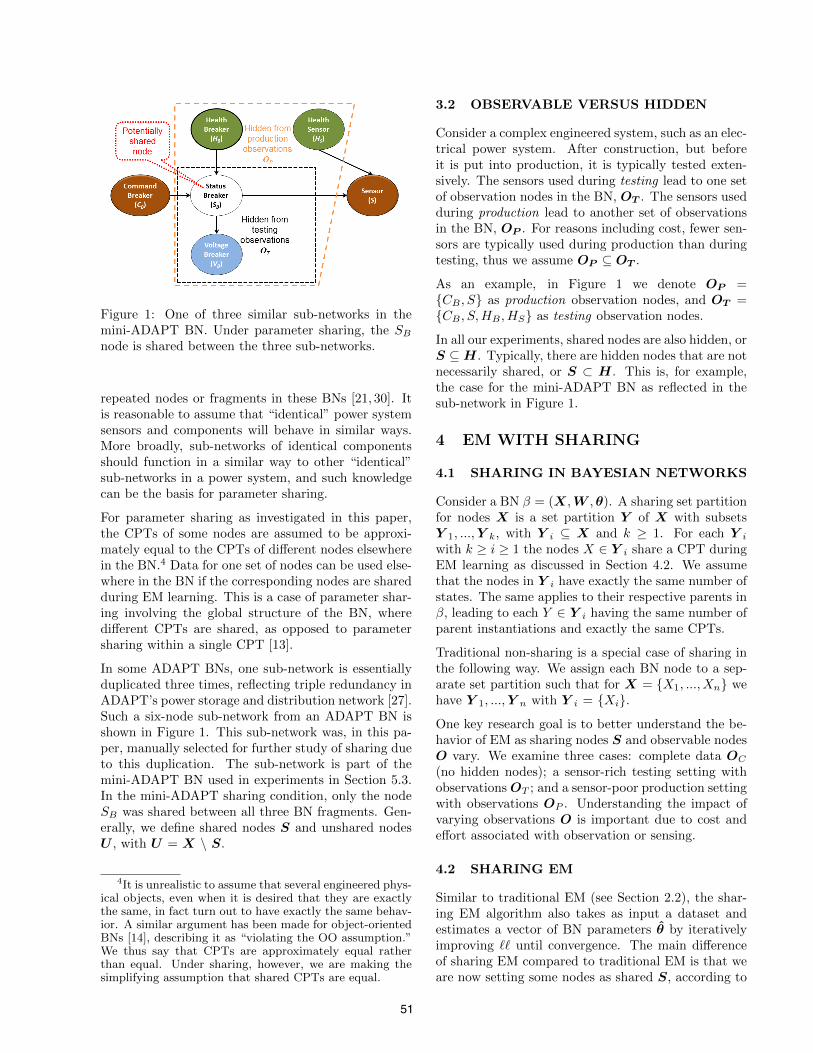
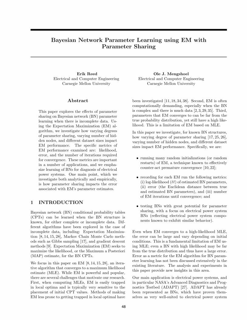
Figure 1: One of three similar sub-networks in themini-ADAPT BN. Under parameter sharing, the S

B

node is shared between the three sub-networks.

repeated nodes or fragments in these BNs [21, 30]. Itis reasonable to assume that “identical” power systemsensors and components will behave in similar ways.More broadly, sub-networks of identical componentsshould function in a similar way to other “identical”sub-networks in a power system, and such knowledgecan be the basis for parameter sharing.

For parameter sharing as investigated in this paper,the CPTs of some nodes are assumed to be approxi-mately equal to the CPTs of di↵erent nodes elsewherein the BN.4 Data for one set of nodes can be used else-where in the BN if the corresponding nodes are sharedduring EM learning. This is a case of parameter shar-ing involving the global structure of the BN, wheredi↵erent CPTs are shared, as opposed to parametersharing within a single CPT [13].

In some ADAPT BNs, one sub-network is essentiallyduplicated three times, reflecting triple redundancy inADAPT’s power storage and distribution network [27].Such a six-node sub-network from an ADAPT BN isshown in Figure 1. This sub-network was, in this pa-per, manually selected for further study of sharing dueto this duplication. The sub-network is part of themini-ADAPT BN used in experiments in Section 5.3.In the mini-ADAPT sharing condition, only the nodeSB

was shared between all three BN fragments. Gen-erally, we define shared nodes S and unshared nodesU , with U = X \ S.

4It is unrealistic to assume that several engineered phys-ical objects, even when it is desired that they are exactlythe same, in fact turn out to have exactly the same behav-ior. A similar argument has been made for object-orientedBNs [14], describing it as “violating the OO assumption.”We thus say that CPTs are approximately equal ratherthan equal. Under sharing, however, we are making thesimplifying assumption that shared CPTs are equal.

3.2 OBSERVABLE VERSUS HIDDEN

Consider a complex engineered system, such as an elec-trical power system. After construction, but beforeit is put into production, it is typically tested exten-sively. The sensors used during testing lead to one setof observation nodes in the BN, OT . The sensors usedduring production lead to another set of observationsin the BN, OP . For reasons including cost, fewer sen-sors are typically used during production than duringtesting, thus we assume OP ✓ OT .

As an example, in Figure 1 we denote OP ={C

B

, S} as production observation nodes, and OT ={C

B

, S,HB

, HS

} as testing observation nodes.

In all our experiments, shared nodes are also hidden, orS ✓ H. Typically, there are hidden nodes that are notnecessarily shared, or S ⇢ H. This is, for example,the case for the mini-ADAPT BN as reflected in thesub-network in Figure 1.

4 EM WITH SHARING

4.1 SHARING IN BAYESIAN NETWORKS

Consider a BN � = (X,W ,✓). A sharing set partitionfor nodes X is a set partition Y of X with subsetsY 1, ...,Y k

, with Yi

✓ X and k � 1. For each Yi

with k � i � 1 the nodes X 2 Yi

share a CPT duringEM learning as discussed in Section 4.2. We assumethat the nodes in Y

i

have exactly the same number ofstates. The same applies to their respective parents in�, leading to each Y 2 Y

i

having the same number ofparent instantiations and exactly the same CPTs.

Traditional non-sharing is a special case of sharing inthe following way. We assign each BN node to a sep-arate set partition such that for X = {X1, ..., Xn

} wehave Y 1, ...,Y n

with Yi

= {Xi

}.

One key research goal is to better understand the be-havior of EM as sharing nodes S and observable nodesO vary. We examine three cases: complete data O

C

(no hidden nodes); a sensor-rich testing setting withobservationsO

T

; and a sensor-poor production settingwith observations O

P

. Understanding the impact ofvarying observations O is important due to cost ande↵ort associated with observation or sensing.

4.2 SHARING EM

Similar to traditional EM (see Section 2.2), the shar-ing EM algorithm also takes as input a dataset andestimates a vector of BN parameters ✓ by iterativelyimproving `` until convergence. The main di↵erenceof sharing EM compared to traditional EM is that weare now setting some nodes as shared S, according to

51

Y . To arrive at the sharing EM algorithm from thetraditional EM algorithm, we modify the likelihoodfunction to introduce parameter sharing and combineparameters (see also [13, 17]). When running sharingEM, nodes X are treated as separate for the E-step.There is a slightly modified M-step, using Y , to ag-gregate the shared CPTs and parameters.5 This is theuse of aggregate su�cient statistics, which considerssu�cient statistics from more than one BN node [13].

Let ✓i,j

be the j’th estimated probability parameter

for BN node Xi

2 X. We define error of ✓ for BN(X,W , ✓) as the L2 distance from the true probabilitydistribution ✓⇤ from which data is sampled:

err(✓) =X

i

sX

j

⇣✓⇤i,j

� ✓i,j

⌘2

. (1)

This error is the summation of the Euclidean distancebetween true and estimated CPT parameters, or theL2 distance, providing an overall distance metric.

Why do we use Euclidean distance to measure error?One could, after all, argue that this distance metricis poor because it does not agree with likelihood. Weuse Euclidean distance because we are interested notonly in the black box performance of the BN, but alsoits validity and understandability to a human expert.6

This is important when an expert needs to evaluate,validate, or refine a BN model, for example a BN foran electrical power system.

4.3 EM’S BEHAVIOR UNDER SHARING

We now provide a simple analysis of certain aspectsof traditional EM (TEM) and sharing EM (SEM). Forsimplicity, we only consider EM runs that convergeand exclude runs that time out.7

For a node Xi

2 X, TEM will converge to one amongpotentially several convergence regions. Suppose thatthe CPT of node X

i

has (Xi

) convergence regions.Then the actual number of convergence regions (�

U

)for a non-shared BN �

U

with nodes X = {X1, ..., Xn

}is upper bounded by (�

U

) as follows:

(�U

) (�U

) =nY

i=1

(Xi

). (2)

5For the relevant LibDAI source code, please seehere: https://github.com/erikreed/HadoopBNEM/blob/master/src/emalg.cpp#L167. In words, it is a modifi-cation on the collection of su�cient statistics during themaximization step.

6We assume that (1) is better than likelihood in thisregard, if the original BN was manually constructed. TheBNs experimented with in Section 5 were manually con-structed, for example.

7In practice, runs that time out are very rare with theparameter settings we use in experiments.

Due to the sharing, SEM intuitively has fewer con-vergence regions than TEM. This is due to SEM’sslightly modified M-step that aggregates the sharedCPTs and parameters. Consider a BN �

S

with ex-actly the same nodes and edges as �

U

, but with shar-ing, specifically with sharing set partitions Y 1, ...,Y k

and k < n. Without loss of generality, assume thatX

i

2 Yi

. Then the actual number of convergence re-gions (�

S

) is upper bounded by (�S

) as follows:

(�S

) (�S

) =kY

i=1

(Xi

), (3)

assuming that the (Xi

) convergence regions used forX

i

in (2) carry over to Yi

.

A special case of (3) is when there exists exactly oneY 0 2 Y such that |Y 0| � 2 while for any Z 2 Y \Y 0 wehave |Z| = 1. The experiments performed in Section 5are all for this special case. Specifically, but withoutloss of generality, let Y

i

= {Xi

} for 1 i < k andY

k

= {Xk

, ..., Xn

} with nS = n� k+1 (i.e., S = Yk

has nS sharing nodes). It is illustrative to consider theratio:

(�U

)

(�S

)=

Qn

i=1 (Xi

)Q

k

i=1 (Xi

)=

nY

i=k+1

(Xi

). (4)

Here, we assume that Xi

has (Xi

) convergence re-gions in both �

U

and �S

and take into account thatfor shared nodes Y

k

= S, CPTs are tied together.

The simple analysis above suggests a non-trivial im-pact of sharing, given the multiplicative e↵ect of the(X

i

)’s for k+1 i n in (4). However, since upperbounds are the focus in this analysis, only a partialand conservative picture is painted. The experimentsin Section 5—see for example Figure 3, Figure 5, andFigure 6—provide further details.

4.4 ANALYSIS OF ERROR

We now consider the number of erroneous CPTs asestimated by SEM when sharing is varied. Clearly, aCPT parameter is continuous and its EM estimate isextremely unlikely to be equal to the original param-eter. Thus we consider here a discrete variable, basedon forming an interval in the one-parameter case. Gen-erally, let a discrete BN nodeX 2 X have k states suchthat x

i

2 {x1, ..., xk

}. Consider ✓xi|z = Pr(X = x

i

|Z = z) for a parent instantiation z. We now have anoriginal CPT parameter ✓

i

2 {✓x1|z, ..., ✓xk�1|z} and

its EM estimate ✓i

2 {✓x1|z, ..., ✓xk�1|z}. Let us jointly

consider the original CPT parameter ✓⇤i

and its esti-mate ✓

i

. If ✓i

2 [✓⇤i

��i

, ✓⇤i

+�i

] we count ✓i

as correct,and say ✓

i

= ✓⇤i

; else it is incorrect or wrong, and we

52

say ✓i

6= ✓⇤i

. This analysis clearly carries over to mul-tiple CPT parameters, parent instantiations, and BNnodes. This shows how we go from a continuous (esti-mated CPT parameters ✓) to a discrete value (numberof wrong or incorrect CPT estimates), where the latteris used in this analysis.

Suppose that up to nP nodes can be shared. Furthersuppose that nS nodes are actually shared while nU

nodes are unshared, with nU + nS = nP . Let TP

be a random variable representing the total numberof wrong or incorrect CPTs, TS the total for sharednodes, and TU the total for unshared nodes. Clearly,we have TP = TS +TU .

Let us first consider the expectation E(TP ). Due tolinearity, we have E(TP ) = E(TS) + E(TU ). In thenon-shared case, assume for simplicity that errors areiid and follow a Bernoulli distribution, with probabilityp of error and (1 � p) = q of no error.8 This givesE(TU ) = nUp, using the fact that a sum of Bernoullirandom variables follows a Binomial distribution.9

In the shared case, all shared nodes either have anincorrect CPT ✓ 6= ✓⇤ or the correct CPT ✓ = ✓⇤.Assuming again probabilities p of error10 and (1�p) =q of no error, and by using the definition of expectationof Binomials we obtain E(TS) = nSp.

Substituting into E(TP ) we get

E(TP ) = nUp+ nSp = nP p. (5)

Let us next consider the variance V (TP ). While vari-ance in general is not linear, we assume linearity forsimplicity, and obtain

V (TP ) = V (TU ) + V (TS). (6)

In the non-shared case we have again a Binomial dis-tribution, with well-known variance

V (TU ) = nUp(1� p). (7)

In the shared case we use the definition of variance,put p1 = (1 � p), p2 = p, and µ = nSp, and obtainafter some simple manipulations:

V (TS) =2X

i=1

pi

(Xi

� µ)2 = n2Sp(1� p), (8)

8This is a simplification, since our use of the Bernoulliassumes that each CPT is either “correct” or “incorrect.”When learned from data, the estimated parameters areclearly almost never exactly correct, but close to or farfrom their respective original values.

9If X is Binomial with parameters n and p, it is well-known that the expected value is E(X) = np.

10The error probabilities of TS and TU are assumed tobe the same as a simplifying assumption.

and by substituting (7) and (8) into (6) we get

V (TP ) = p(1� p)((nP � nS) + n2S). (9)

In words, (9) tells us that as the number nS of sharednodes increases at the expense of the number of un-shared nodes nU , variance due to non-shared nodes de-creases linearly, but variance due to sharing increasesquadratically. The net e↵ect shown in (9) is that vari-ance V (TP ) of the error increases with the number ofshared nodes, according to our analysis above. Ex-pectation, on the other hand, remains constant (5)regardless of how many nodes are shared. These ana-lytical results have empirical counterparts as discussedin Section 5, see for example the error sub-plot at thebottom of Figure 2.

5 EXPERIMENTS

We now report on EM experiments for several di↵er-ent BNs, using varying degrees of sharing. We alsovary the number of hidden nodes and dataset size. Weused ✏ = 1e�3 as an EM convergence criterion, mean-ing that EM stopped at iteration t0 when the ``-scorechanged by a value ✏ between iterations t0�1 and t0

for tmax � t0 � tmin. In these experiments, tmax = 100and tmin = 3.

5.1 METHODS AND DATA

Bayesian networks. Table 2 presents BNs used inthe experiments.11 Except for the BN Pigs, these BNsall represent (parts of) the ADAPT electrical powersystem (see Section 3). The BN Pigs has the largestnumber of nodes that can be shared (nP = 296), com-prising 67% of the entire BN. The largest BN used,in terms of node count, edges, and total CPT size, isADAPT T2.

Datasets. Data for EM learning of parameters forthese BNs were generated using forward sampling.12

Each sample in a dataset is a vector x (see Section 2.1).The larger BNs were tested with increasing numbersof samples ranging from 25 to 400, while mini-ADAPTwas tested with 25 to 2000 samples.

Sharing. Each BN has a di↵erent number of param-eters that can be shared, where a set of nodes Y

i

211ADAPT BNs can be found here: http://works.

bepress.com/ole_mengshoel/.12Our experiments are limited in that we are only learn-

ing the parameters of BNs, using data generated from thoseBNs. Clearly, in most applications, data is not generatedfrom a BN and the true distribution does not conform ex-actly to some BN structure. However, our analytical andexperimental investigation of error would not have beenpossible without this simplifying assumption.

53

NAME |X| |P | |W | CPT

ADAPT T1 120 26 136 1504ADAPT T2 671 107 789 13281ADAPT P1 172 33 224 4182ADAPT P2 494 99 602 10973mini-ADAPT 18 3 15 108Pigs 441 296 592 8427

Table 2: Bayesian networks used in experiments. The|P | column presents the number of potentially sharednodes, with actually shared nodes S ✓ P . The CPTcolumn denotes the total number of parameters in theconditional probability tables.

Y with equal CPTs are deemed sharable. In mostcases, there were multiple sets of nodes Y 1, ..., Y

k

with |Yi

| � 2 for k � i � 1. When multiple sets wereavailable, the largest set was selected for experimenta-tion, as shown in Section 5.2’s pseudo-code.

Metrics. After an EM trial converged to an estimate✓, we collected the following three metrics:

1. number of iterations t0 needed to converge to ✓,

2. log-likelihood `` of ✓, and

3. error: distance between ✓ and the original ✓⇤ (see(1) for the definition).

To provide reliable statistics on mean and standarddeviation, many randomly initialized EM trials wererun.

Software. Among the available software implementa-tions of the EM algorithm for BNs, we have based ourwork on LibDAI [23].13 LibDAI uses factor graphs forits internal representation of BNs, and has several BNinference algorithms implemented. During EM, theexact junction tree inference algorithm [16] was used,since it has performed well previously [19].

5.2 VARYING NUMBER OF SHAREDNODES

Here we investigate how varying the number of sharednodes impacts EM. A set of hidden nodes H was cre-ated for each BN by selecting

H = argmaxY i2Y

|Yi

|,

where Y is a sharing set partition for BN nodes X(see Section 4.1). In other words, each experimentalBN had its largest set of shareable nodes hidden, giv-ing nH = 12 nodes for ADAPT T1, nH = 66 nodesfor ADAPT T2, nH = 32 nodes for ADAPT P1, andnH = 145 nodes for Pigs.

13www.libdai.org

The following gradual sharing method is used to varysharing. Given a fixed set of hidden nodes H and aninitially empty set of shared nodes S:

1. Randomly add �nS � 1 hidden nodes that arenot yet shared to the set of shared nodes S. Sincewe only have a single sharing set, this means mov-ing �nS nodes from the set H \ S to the set S.

2. Performm sharing EM trials in this configuration,and record the three metrics for each trial.

3. Repeat until all hidden nodes are shared; that is,S = H.

Using the gradual sharing method above, BN nodeswere picked as hidden and then gradually shared.When increasing the number of shared nodes, the newset of shared nodes was a superset of the previous set,and a certain number of EM trials was performed foreach set.

5.2.1 One Network

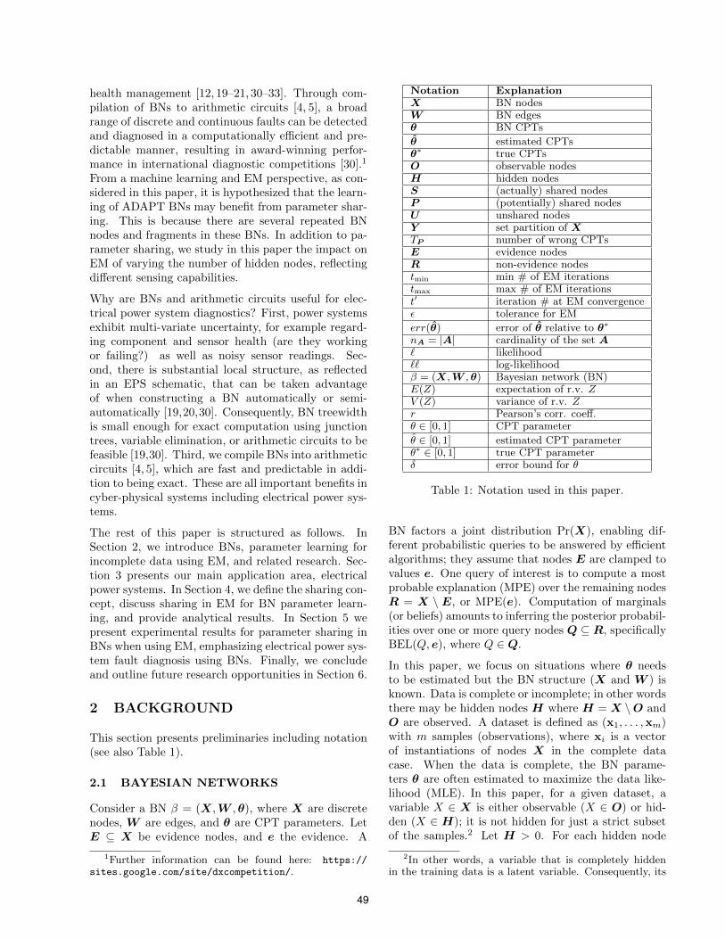
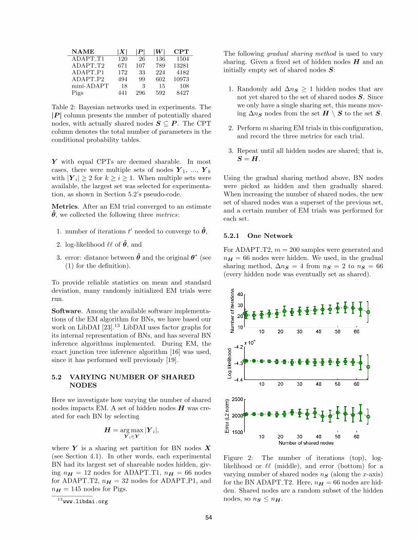
For ADAPT T2, m = 200 samples were generated andnH = 66 nodes were hidden. We used, in the gradualsharing method, �nS = 4 from nS = 2 to nS = 66(every hidden node was eventually set as shared).

Figure 2: The number of iterations (top), log-likelihood or `` (middle), and error (bottom) for avarying number of shared nodes nS (along the x-axis)for the BN ADAPT T2. Here, nH = 66 nodes are hid-den. Shared nodes are a random subset of the hiddennodes, so nS nH .

54

ADAPT T1Iterations Likelihood Error

Size r(µ) r(�) r(µ) r(�) r(µ) r(�)25 -0.937 -0.135 0.997 0.882 -0.068 0.88850 -0.983 -0.765 0.992 0.941 0.383 0.988

100 -0.825 0.702 0.494 0.941 0.786 0.985200 0.544 0.926 -0.352 0.892 0.517 0.939400 0.810 0.814 -0.206 0.963 0.863 0.908

ADAPT T2Iterations Likelihood Error

Size r(µ) r(�) r(µ) r(�) r(µ) r(�)25 0.585 0.852 0.749 0.842 0.276 0.99750 0.811 0.709 0.377 0.764 0.332 0.981

100 0.772 0.722 -0.465 0.855 -0.387 0.992200 0.837 0.693 -0.668 0.788 -0.141 0.989400 0.935 0.677 -0.680 0.784 -0.0951 0.987

ADAPT P1Iterations Likelihood Error

Size r(µ) r(�) r(µ) r(�) r(µ) r(�)25 -0.769 -0.0818 -0.926 0.278 -0.107 0.77450 -0.864 -0.0549 -0.939 0.218 -0.331 0.188

100 -0.741 0.436 -0.871 0.678 -0.458 0.457200 -0.768 0.408 -0.879 0.677 -0.196 0.700400 -0.665 0.560 -0.862 0.681 0.00444 0.653

PIGSIterations Likelihood Error

Size r(µ) r(�) r(µ) r(�) r(µ) r(�)25 0.954 0.763 0.970 0.614 0.965 0.88750 0.966 0.956 0.137 0.908 0.740 0.869

100 -0.922 -0.0167 -0.994 -0.800 -0.893 0.343200 -0.827 -0.394 -0.985 -0.746 -0.577 0.0157400 -0.884 -0.680 -0.942 -0.699 -0.339 0.285

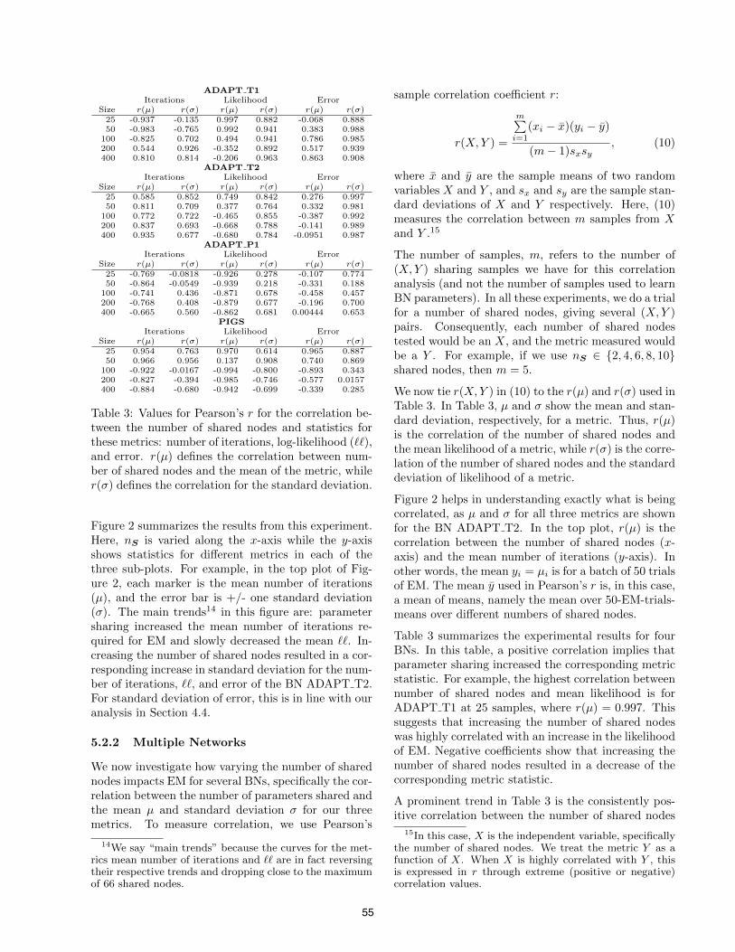
Table 3: Values for Pearson’s r for the correlation be-tween the number of shared nodes and statistics forthese metrics: number of iterations, log-likelihood (``),and error. r(µ) defines the correlation between num-ber of shared nodes and the mean of the metric, whiler(�) defines the correlation for the standard deviation.

Figure 2 summarizes the results from this experiment.Here, nS is varied along the x-axis while the y-axisshows statistics for di↵erent metrics in each of thethree sub-plots. For example, in the top plot of Fig-ure 2, each marker is the mean number of iterations(µ), and the error bar is +/- one standard deviation(�). The main trends14 in this figure are: parametersharing increased the mean number of iterations re-quired for EM and slowly decreased the mean ``. In-creasing the number of shared nodes resulted in a cor-responding increase in standard deviation for the num-ber of iterations, ``, and error of the BN ADAPT T2.For standard deviation of error, this is in line with ouranalysis in Section 4.4.

5.2.2 Multiple Networks

We now investigate how varying the number of sharednodes impacts EM for several BNs, specifically the cor-relation between the number of parameters shared andthe mean µ and standard deviation � for our threemetrics. To measure correlation, we use Pearson’s

14We say “main trends” because the curves for the met-rics mean number of iterations and `` are in fact reversingtheir respective trends and dropping close to the maximumof 66 shared nodes.

sample correlation coe�cient r:

r(X,Y ) =

mPi=1

(xi

� x)(yi

� y)

(m� 1)sx

sy

, (10)

where x and y are the sample means of two randomvariables X and Y , and s

x

and sy

are the sample stan-dard deviations of X and Y respectively. Here, (10)measures the correlation between m samples from Xand Y .15

The number of samples, m, refers to the number of(X,Y ) sharing samples we have for this correlationanalysis (and not the number of samples used to learnBN parameters). In all these experiments, we do a trialfor a number of shared nodes, giving several (X,Y )pairs. Consequently, each number of shared nodestested would be an X, and the metric measured wouldbe a Y . For example, if we use nS 2 {2, 4, 6, 8, 10}shared nodes, then m = 5.

We now tie r(X,Y ) in (10) to the r(µ) and r(�) used inTable 3. In Table 3, µ and � show the mean and stan-dard deviation, respectively, for a metric. Thus, r(µ)is the correlation of the number of shared nodes andthe mean likelihood of a metric, while r(�) is the corre-lation of the number of shared nodes and the standarddeviation of likelihood of a metric.

Figure 2 helps in understanding exactly what is beingcorrelated, as µ and � for all three metrics are shownfor the BN ADAPT T2. In the top plot, r(µ) is thecorrelation between the number of shared nodes (x-axis) and the mean number of iterations (y-axis). Inother words, the mean y

i

= µi

is for a batch of 50 trialsof EM. The mean y used in Pearson’s r is, in this case,a mean of means, namely the mean over 50-EM-trials-means over di↵erent numbers of shared nodes.

Table 3 summarizes the experimental results for fourBNs. In this table, a positive correlation implies thatparameter sharing increased the corresponding metricstatistic. For example, the highest correlation betweennumber of shared nodes and mean likelihood is forADAPT T1 at 25 samples, where r(µ) = 0.997. Thissuggests that increasing the number of shared nodeswas highly correlated with an increase in the likelihoodof EM. Negative coe�cients show that increasing thenumber of shared nodes resulted in a decrease of thecorresponding metric statistic.

A prominent trend in Table 3 is the consistently pos-itive correlation between the number of shared nodes

15In this case, X is the independent variable, specificallythe number of shared nodes. We treat the metric Y as afunction of X. When X is highly correlated with Y , thisis expressed in r through extreme (positive or negative)correlation values.

55

NO SHARINGObservable Error Likelihood Iterations

µ � µ � µ �

OC 16.325 (-) -3.047e4 (-) (-) (-)OP 48.38 3.74 -2.009e4 43.94 16.39 4.98OT 33.25 7.45 -2.492e4 1190 8.65 1.99

SHARINGObservable Error Likelihood Iterations

µ � µ � µ �

OC 16.323 (-) -3.047e4 (-) (-) (-)OP 48.56 3.92 -2.010e4 62.87 15.98 4.95OT 34.12 14.3 -2.629e4 2630 6.59 2.48

Table 4: Comparison of No Sharing (top) versus Shar-ing (bottom) for di↵erent observable node sets O

C

,O

P

, and OT

during 600 EM trials for mini-ADAPT.

nS and the standard deviation of error, r(�), for all 4BNs. This is in line with the analytical result involvingnS in (9).

The number of samples was shown to have a signifi-cant impact on these correlations. The Pigs networkshowed a highly correlated increase in the mean num-ber of iterations for 25 and 50 samples. However, for100, 200, and 400 samples there was a decrease in themean number of iterations. The opposite behavior isobserved in ADAPT T1, where fewer samples resultedin better performance for parameter sharing (reducingthe mean number of iterations), while for 200 and 400samples we found that parameter sharing increased themean number of iterations. Further experimentationand analysis may improve the understanding of the in-teraction between sharing and the number of samples.

5.3 CONVERGENCE REGIONS

5.3.1 Small Bayesian Networks

First, we will show how sharing influences EM parame-ter interactions for the mini-ADAPT BN shown in Fig-ure 1 and demonstrate how shared parameters jointlyconverge.

Earlier we introduced OP

as observable nodes in aproduction system and O

T

as observable nodes in atesting system. Complementing O

P

, hidden nodes areH

P

= {HB

, HS

, VB

, SB

}. Complementing OT

, hid-den nodes are H

T

= {VB

, SB

}. When a node is hid-den, the EM algorithm will converge to one among itspotentially many convergence regions. For O

P

, EMhad much less observed data to work with than for O

T

(see Figure 1). For OP

, the health breaker node HB

was, for instance, not observed or even connected toany nodes that were observed. In contrast, O

T

was de-signed to allow better observation of the components’behaviors, and H

B

2 OT

. From mini-ADAPT, 500samples were generated. Depending on the observableset used, either nH = |H

T

| = 2 or nH = |HP

| = 4nodes were hidden, and 600 random EM trials were

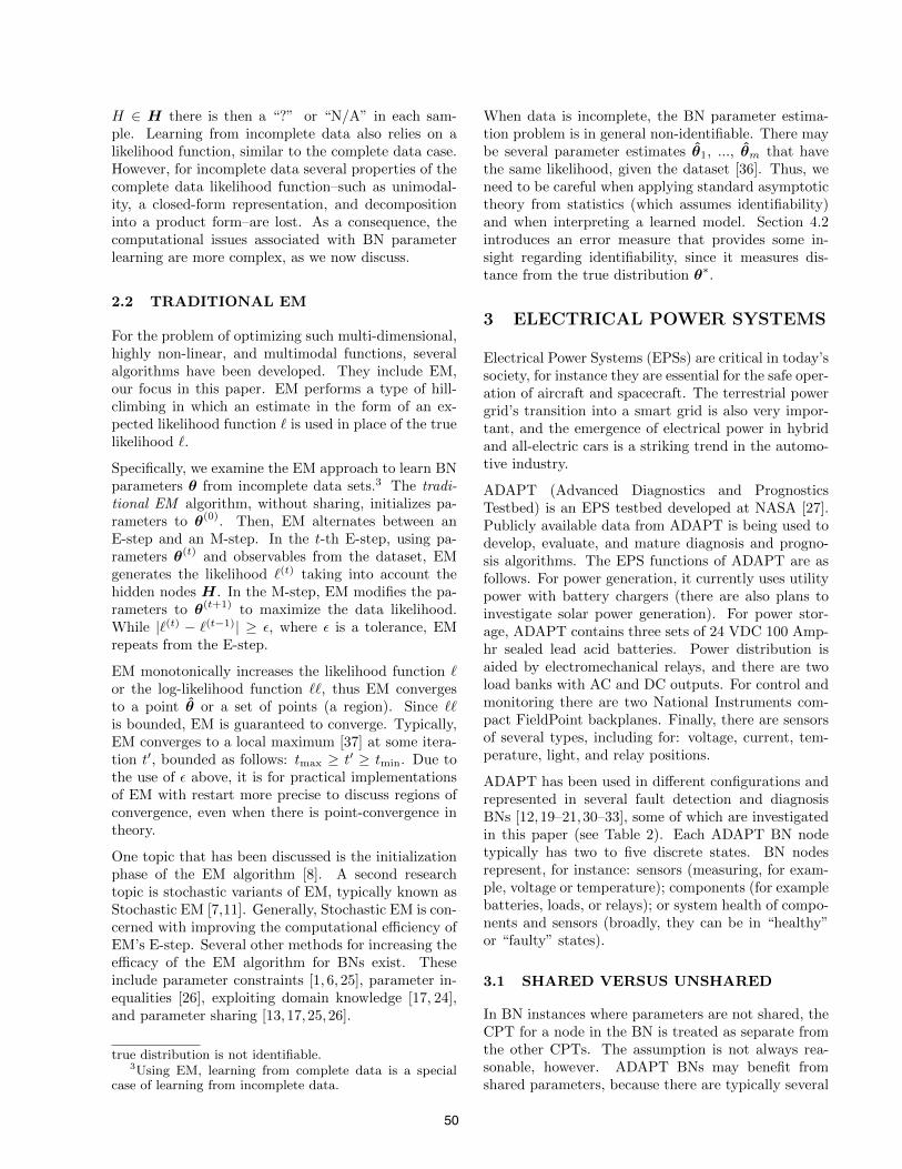
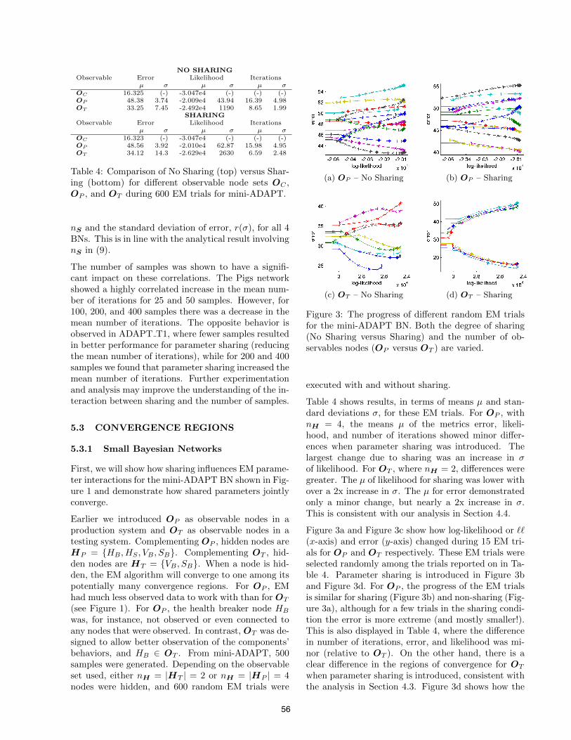
(a) OP – No Sharing (b) OP – Sharing

(c) OT – No Sharing (d) OT – Sharing

Figure 3: The progress of di↵erent random EM trialsfor the mini-ADAPT BN. Both the degree of sharing(No Sharing versus Sharing) and the number of ob-servables nodes (O

P

versus OT

) are varied.

executed with and without sharing.

Table 4 shows results, in terms of means µ and stan-dard deviations �, for these EM trials. For O

P

, withnH = 4, the means µ of the metrics error, likeli-hood, and number of iterations showed minor di↵er-ences when parameter sharing was introduced. Thelargest change due to sharing was an increase in �of likelihood. For O

T

, where nH = 2, di↵erences weregreater. The µ of likelihood for sharing was lower withover a 2x increase in �. The µ for error demonstratedonly a minor change, but nearly a 2x increase in �.This is consistent with our analysis in Section 4.4.

Figure 3a and Figure 3c show how log-likelihood or ``(x-axis) and error (y-axis) changed during 15 EM tri-als for O

P

and OT

respectively. These EM trials wereselected randomly among the trials reported on in Ta-ble 4. Parameter sharing is introduced in Figure 3band Figure 3d. For O

P

, the progress of the EM trialsis similar for sharing (Figure 3b) and non-sharing (Fig-ure 3a), although for a few trials in the sharing condi-tion the error is more extreme (and mostly smaller!).This is also displayed in Table 4, where the di↵erencein number of iterations, error, and likelihood was mi-nor (relative to O

T

). On the other hand, there is aclear di↵erence in the regions of convergence for O

T

when parameter sharing is introduced, consistent withthe analysis in Section 4.3. Figure 3d shows how the

56

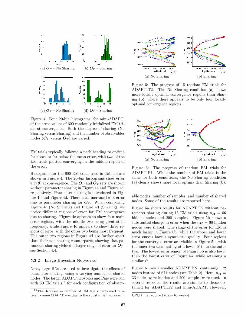
(a) OP – No Sharing (b) OP – Sharing

(c) OT – No Sharing (d) OT – Sharing

Figure 4: Four 20-bin histograms, for mini-ADAPT,of the error values of 600 randomly initialized EM tri-als at convergence. Both the degree of sharing (NoSharing versus Sharing) and the number of observablesnodes (O

P

versus OT

) are varied.

EM trials typically followed a path heading to optimafar above or far below the mean error, with two of theEM trials plotted converging in the middle region ofthe error.

Histograms for the 600 EM trials used in Table 4 areshown in Figure 4. The 20-bin histograms show errorerr(✓) at convergence. TheO

P

andOT

sets are shownwithout parameter sharing in Figure 4a and Figure 4c,respectively. Parameter sharing is introduced in Fig-ure 4b and Figure 4d. There is an increased � of errordue to parameter sharing for O

T

. When comparingFigure 4c (No Sharing) and Figure 4d (Sharing), wenotice di↵erent regions of error for EM convergencedue to sharing. Figure 4c appears to show four mainerror regions, with the middle two being greatest infrequency, while Figure 4d appears to show three re-gions of error, with the outer two being most frequent.The outer two regions in Figure 4d are further apartthan their non-sharing counterparts, showing that pa-rameter sharing yielded a larger range of error for O

T

,see Section 4.4.

5.3.2 Large Bayesian Networks

Next, large BNs are used to investigate the e↵ects ofparameter sharing, using a varying number of sharednodes. The larger ADAPT networks and Pigs were runwith 50 EM trials16 for each configuration of observ-

16The decrease in number of EM trials performed rela-tive to mini-ADAPT was due to the substantial increase in

(a) No Sharing (b) Sharing

Figure 5: The progress of 15 random EM trials forADAPT T2. The No Sharing condition (a) showsmore locally optimal convergence regions than Shar-ing (b), where there appears to be only four locallyoptimal convergence regions.

(a) No Sharing (b) Sharing

Figure 6: The progress of random EM trials forADAPT P1. While the number of EM trials is thesame for both conditions, the No Sharing condition(a) clearly shows more local optima than Sharing (b).

able nodes, number of samples, and number of sharednodes. Some of the results are reported here.

Figure 5a shows results for ADAPT T2 without pa-rameter sharing during 15 EM trials using nH = 66hidden nodes and 200 samples. Figure 5b shows asubstantial change in error when the nH = 66 hiddennodes were shared. The range of the error for EM ismuch larger in Figure 5b, while the upper and lowererror curves have a symmetric quality. Four regionsfor the converged error are visible in Figure 5b, withthe inner two terminating at a lower `` than the outertwo. The lowest error region of Figure 5b is also lowerthan the lowest error of Figure 5a, while retaining asimilar ``.

Figure 6 uses a smaller ADAPT BN, containing 172nodes instead of 671 nodes (see Table 2). Here, nH =33 nodes were hidden and 200 samples were used. Inseveral respects, the results are similar to those ob-tained for ADAPT T2 and mini-ADAPT. However,

CPU time required (days to weeks).

57

Figure 6a shows that EM terminates on di↵erent like-lihoods, which is not observed in Figure 5a. The erroralso appears to generally fluctuate more in Figure 6a,whereas the error changes the most during later it-erations in Figure 5a. Figure 6b applies parametersharing to the nH = 33 hidden nodes. A symmetrice↵ect is visible between high and low error, reflect-ing the analysis in Section 4. Of the 15 trials shownin Figure 6b, two attained `` > �1.2e�4, while therest converged at `` ⇡ �1.21e�4. Additionally, the``s of these two trials were greater than any of thenon-sharing ``s shown in Figure 6a.

6 CONCLUSION

Bayesian networks have proven themselves as verysuitable for electrical power system diagnostics [19,20,30–33]. By compiling Bayesian networks to arithmeticcircuits [4,5], a broad range of discrete and continuousfaults can be handled in a computationally e�cientand predictable manner. This approach has resultedin award-winning performance on public data fromADAPT, an electrical power system at NASA [30].

The goal of this paper is to investigate the e↵ect, onEM’s behavior, of parameter sharing in Bayesian net-works. We emphasize electrical power systems as anapplication, and in particular examine EM for ADAPTBayesian networks. In these networks, there is consid-erable opportunity for parameter sharing.

Our results suggest complex interactions betweenvarying degrees of parameter sharing, varying numberof hidden nodes, and di↵erent dataset sizes when itcomes to impact on EM performance, specifically like-lihood, error, and the number of iterations required forconvergence. One main point, which we investigatedboth analytically and empirically, is how parametersharing impacts the error associated with EM’s pa-rameter estimates. In particular, we have found an-alytically that the error variance increases with thenumber of shared parameters. Experiments with sev-eral BNs, mostly for fault diagnosis of electrical powersystems, are in line with the analysis. The good newshere is that there is, in the sharing case, smaller errorsome of the time.

Further theoretical research to better understand pa-rameter sharing is required. Since parameter sharingwas demonstrated to perform poorly in certain cases,further investigations appear promising. Parametersharing sometimes reduced the number of EM itera-tions required for parameter learning, while at othertimes the number of EM iterations increases. Improv-ing the understanding of the joint impact of parametersharing and the number of samples on the number ofEM iterations would be useful, for example. Finally, it

would be interesting to investigate the connection toobject-oriented and relational BNs in future work.

References

[1] E.E. Altendorf, A.C. Restificar, and T.G. Dietterich.Learning from sparse data by exploiting monotonicityconstraints. In Proceedings of UAI, volume 5, 2005.

[2] A. Basak, I. Brinster, X. Ma, and O. J. Mengshoel.Accelerating Bayesian network parameter learning us-ing Hadoop and MapReduce. In Proc. of BigMine-12,Beijing, China, August 2012.

[3] P.S. Bradley, U. Fayyad, and C. Reina. ScalingEM (Expectation-Maximization) clustering to largedatabases. Microsoft Research Report, MSR-TR-98-35, 1998.

[4] M. Chavira and A. Darwiche. Compiling Bayesiannetworks with local structure. In Proceedings of the19th International Joint Conference on Artificial In-telligence (IJCAI), pages 1306–1312, 2005.

[5] A. Darwiche. A di↵erential approach to inference inBayesian networks. Journal of the ACM, 50(3):280–305, 2003.

[6] C.P. de Campos and Q. Ji. Improving Bayesian net-work parameter learning using constraints. In Proc.19th International Conference on Pattern Recognition(ICPR), pages 1–4. IEEE, 2008.

[7] B. Delyon, M. Lavielle, and E. Moulines. Convergenceof a stochastic approximation version of the EM algo-rithm. Annals of Statistics, (27):94–128, 1999.

[8] A. P. Dempster, N. M. Laird, and D. B. Rubin. Max-imum likelihood from incomplete data via the EM al-gorithm. Journal Of The Royal Statistical Society,Series B, 39(1):1–38, 1977.

[9] R. Greiner, X. Su, B. Shen, and W. Zhou. Struc-tural extension to logistic regression: Discriminativeparameter learning of belief net classifiers. MachineLearning, 59(3):297–322, 2005.

[10] S.H. Jacobson and E. Yucesan. Global optimizationperformance measures for generalized hill climbing al-gorithms. Journal of Global Optimization, 29(2):173–190, 2004.

[11] W. Jank. The EM algorithm, its randomized imple-mentation and global optimization: Some challengesand opportunities for operations research. In F. B.Alt, M. C. Fu, and B. L. Golden, editors, Perspectivesin Operations Research: Papers in Honor of Saul Gass80th Birthday. Springer, 2006.

[12] W. B. Knox and O. J. Mengshoel. Diagnosis and re-configuration using Bayesian networks: An electricalpower system case study. In Proc. of the IJCAI-09Workshop on Self-? and Autonomous Systems (SAS):Reasoning and Integration Challenges, pages 67–74,2009.

[13] D. Koller and N. Friedman. Probabilistic graphicalmodels: principles and techniques. The MIT Press,2009.

58

[14] H. Langseth and O. Bangsø. Parameter learningin object-oriented Bayesian networks. Annals ofMathematics and Artificial Intelligence, 32(1):221–243, 2001.

[15] S.L. Lauritzen. The EM algorithm for graphical as-sociation models with missing data. ComputationalStatistics & Data Analysis, 19(2):191–201, 1995.

[16] S.L. Lauritzen and D.J. Spiegelhalter. Local compu-tations with probabilities on graphical structures andtheir application to expert systems. Journal of theRoyal Statistical Society. Series B (Methodological),pages 157–224, 1988.

[17] W. Liao and Q. Ji. Learning Bayesian network param-eters under incomplete data with domain knowledge.Pattern Recognition, 42(11):3046–3056, 2009.

[18] G.J. McLachlan and D. Peel. Finite mixture models.Wiley, 2000.

[19] O. J. Mengshoel, M. Chavira, K. Cascio, S. Poll,A. Darwiche, and S. Uckun. Probabilistic model-based diagnosis: An electrical power system casestudy. IEEE Trans. on Systems, Man, and Cyber-netics, 40(5):874–885, 2010.

[20] O. J. Mengshoel, A. Darwiche, K. Cascio, M. Chavira,S. Poll, and S. Uckun. Diagnosing faults in electricalpower systems of spacecraft and aircraft. In Proceed-ings of the Twentieth Innovative Applications of Arti-ficial Intelligence Conference (IAAI-08), pages 1699–1705, Chicago, IL, 2008.

[21] O. J. Mengshoel, S. Poll, and T. Kurtoglu. Devel-oping large-scale Bayesian networks by composition:Fault diagnosis of electrical power systems in aircraftand spacecraft. In Proc. of the IJCAI-09 Workshopon Self-? and Autonomous Systems (SAS): Reasoningand Integration Challenges, pages 59–66, 2009.

[22] O.J. Mengshoel, D.C. Wilkins, and D. Roth. Initial-ization and restart in stochastic local search: Com-puting a most probable explanation in Bayesian net-works. IEEE Transactions on Knowledge and DataEngineering, 23(2):235–247, 2011.

[23] J.M. Mooij. libDAI: A free and open source C++library for discrete approximate inference in graphi-cal models. Journal of Machine Learning Research,11:2169–2173, August 2010.

[24] S. Natarajan, P. Tadepalli, E. Altendorf, T.G. Diet-terich, A. Fern, and A.C. Restificar. Learning first-order probabilistic models with combining rules. InICML, pages 609–616, 2005.

[25] R.S. Niculescu, T.M. Mitchell, and R.B. Rao.Bayesian network learning with parameter con-straints. The Journal of Machine Learning Research,7:1357–1383, 2006.

[26] R.S. Niculescu, T.M. Mitchell, and R.B. Rao. Atheoretical framework for learning Bayesian networkswith parameter inequality constraints. In Proc. of the20th International Joint Conference on Artifical Intel-ligence, pages 155–160, 2007.

[27] S. Poll, A. Patterson-Hine, J. Camisa, D. Gar-cia, D. Hall, C. Lee, O.J. Mengshoel, C. Neukom,D. Nishikawa, J. Ossenfort, A. Sweet, S. Yen-tus, I. Roychoudhury, M. Daigle, G. Biswas, andX. Koutsoukos. Advanced diagnostics and prognosticstestbed. In Proc. of the 18th International Workshopon Principles of Diagnosis (DX-07), pages 178–185,2007.

[28] M. Ramoni and P. Sebastiani. Robust learning withmissing data. Machine Learning, 45(2):147–170, 2001.

[29] E. Reed and O.J. Mengshoel. Scaling Bayesiannetwork parameter learning with expectation maxi-mization using MapReduce. Proc. of Big LearningWorkshop on Neural Information Processing Systems(NIPS-12), 2012.

[30] B. Ricks and O. J. Mengshoel. Diagnosis for uncertain,dynamic and hybrid domains using Bayesian networksand arithmetic circuits. International Journal of Ap-proximate Reasoning, 55(5):1207–1234, 2014.

[31] B. W. Ricks, C. Harrison, and O. J. Mengshoel. In-tegrating probabilistic reasoning and statistical qual-ity control techniques for fault diagnosis in hybriddomains. In In Proc. of the Annual Conference ofthe Prognostics and Health Management Society 2011(PHM-11), Montreal, Canada, 2011.

[32] B. W. Ricks and O. J. Mengshoel. Methods for prob-abilistic fault diagnosis: An electrical power systemcase study. In Proc. of Annual Conference of the PHMSociety, 2009 (PHM-09), San Diego, CA, 2009.

[33] B. W. Ricks and O. J. Mengshoel. Diagnosing in-termittent and persistent faults using static Bayesiannetworks. In Proc. of the 21st International Work-shop on Principles of Diagnosis (DX-10), Portland,OR, 2010.

[34] A. Saluja, P.K. Sundararajan, and O.J. Mengshoel.Age-Layered Expectation Maximization for parameterlearning in Bayesian Networks. In Proceedings of Arti-ficial Intelligence and Statistics (AIStats), La Palma,Canary Islands, 2012.

[35] B. Thiesson, C. Meek, and D. Heckerman. Accel-erating EM for large databases. Machine Learning,45(3):279–299, 2001.

[36] S. Watanabe. Algebraic analysis for nonidentifiablelearning machines. Neural Computation, 13(4):899–933, 2001.

[37] C.F. Wu. On the convergence properties of the EM al-gorithm. The Annals of Statistics, 11(1):95–103, 1983.

[38] Z. Zhang, B.T. Dai, and A.K.H. Tung. Estimating lo-cal optimums in EM algorithm over Gaussian mixturemodel. In Proc. of the 25th international conferenceon Machine learning, pages 1240–1247. ACM, 2008.

59