bayesian persuasion with optimal learningy
TRANSCRIPT

Bayesian Persuasion with Optimal Learning†
Xiaoye Liao‡
New York University
Abstract
We study a model of Bayesian persuasion between a designer and a receiver with
one substantial deviation—the receiver can acquire costly i.i.d. signals from the offered
information structure. Taking a 2-state-2-action environment as the baseline and using
continuous approximation, we fully characterize the optimal persuasion policy. When
the receiver features high skepticism, the optimal policy is to immediately reveal the
truth, which is true for an unexpectedly large set of primitives. We locate the designer’s
maximum payoff, find the setup cost of persuasion the designer incurs, and identify a
wedge that measures the value of dictating information acquisition for the designer. Some
extensions of the baseline model are discussed.
Keywords: Bayesian persuasion, optimal learning, continuous approximation
JEL Classifications: D82, D83
†First draft: May 2015; This draft: September 2019.‡Email: [email protected]. I am indebted to Ennio Stacchetti and Laurent Mathevet for their dedication and
tolerance. I am grateful to Rene Caldentey and Debraj Ray for helpful comments and suggestions.
1

1 Introduction
Imagine that a scientific journal editor receives from a researcher an article claiming a discovery
that is reproducible via an experiment. The researcher wants to find her way into publication,
but the editor must assess the reliability of the finding, and will make a decision, accepting
or rejecting, only after ample evidence has been collected from sufficient repetition of the
experiment. How should the researcher optimally design her experiment?
Similar examples are abundant. While prosecutors aim at conviction, judges may require
multiple independent investigations to reach a sufficient level of convincement; while producers
just want to make sales, consumers are usually allowed to try products for a certain length of
time before purchase. In these scenarios, people with the authority to decide (receivers) make
use of information potentially manipulated by those with expertise and different interests
(designers). However, unlike those typically modeled in communication games, receivers
are not “passive audiences”, they instead get a say through dictating the utilization of the
information sources offered by the designers. This paper analyzes the extent to which such a
protocol will reshape our insight into strategic information transmission with commitment.
To this end, the communication problem is modeled as a Bayesian persuasion game with
one substantive divergence from its paradigm. The receiver (he) faces a binary decision
problem with incomplete information on a constant state. The designer (she), uninformed
about the state ex ante, cares about the receiver’s action and can influence it by communicating
with him via committed signals. In particular, the designer provides once and for all, at the
outset, an information structure with commitment, from which the receiver is allowed to draw
as many (conditionally) independent signals as he desires over an infinite horizon. Potentially
becoming more informed, the receiver must weigh the informational benefits against the
opportunity cost of information acquisition. The costs have the most parsimonious form:
The receiver is impatient while information is collected via time-consuming sequential tests.
In the baseline setting, agents share a common belief on a binary state, and the designer’s
preferences are time and state-independent. By choosing the format of her persuasion, the
designer maximizes the probability that the receiver ends up with her preferred action.
We follow the belief-based approach and represent communication by its induced informa-
tion policy, which is a distribution of receiver posteriors generated by an optimally stopped
belief martingale in discrete time. The distribution necessarily averages back to the prior, but
Bayes plausibility alone fails to capture the receiver’s incentive compatibility in learning. A
sufficient yet tractable characterization of the receiver’s optimal stopping policy, and how its
outcome — the distribution of stopping posteriors, i.e., those at which information acquisition
is terminated — relies on the designer’s strategy, is thus in needed. This creates new challenges
along a couple of fronts.
The first challenge lies in determining the optimal signal space. In most Bayesian persuasion
2

literature, signals can be treated as action recommendations to receivers, and so we can equate
the signal space for each receiver and the set of his feasible actions. Such “revelation principle”,
however, fails to hold in our setup for two reasons: Due to endogenous information acquisition,
a signal might induce more information acquisition in the early stages but terminate it later
in sequential tests. Moreover, the number of stopping posteriors is in general independent
to the signal space and hence gives no clue about the latter. The second challenge is to
derive the distribution of an optimally stopped belief martingale generated by an information
structure in sequential tests, which plays a pivotal role in our model; the major difficulty
is owing to the discreteness and asymmetry of belief updating. One may wonder if we can
circumvent those difficulties by focusing on static information structures, i.e., those which
induce only one-shot learning, which restores the revelation principle and avoids addressing
the dynamic information acquisition problem. A two-period numerical example presented in
the online appendix, however, proves this conjecture problematic. Multiple random draws,
as illustrated there, could be in the interest of the designer, rendering the static solution
suboptimal.
Instead, the central tool we employ is a continuous approximation. We collapse a discrete
lump-sum belief updating into a sub-dynamic process so that belief renews continuously. In
the limit, a nonnegative number, interpreted as informational accuracy, summarizes the role
an information structure plays on belief evolution. The approximation enables us to formulate
the receiver’s problem as an optimal diffusion control, which admits a closed-form cutoff policy
that maps each information structure to a pair of stopping posteriors. Each stopping posterior
identifies a class of information structures with the same limit accuracy, and the range of the
stopping posteriors as accuracy varies constitutes the feasible set and represents information.
Encapsulating the receiver’s incentive compatibility, the information representation, unlike
its counterpart in the one-shot learning benchmark (“1-benchmark” hereafter for simplicity),
degenerates to a curve, that is, the designer can choose only one of the two stopping posteriors.
In other words, to meet the receiver’s incentive compatibility, the designer has to give up one
degree of freedom in her decision as compared to the 1-benchmark. Moreover, the information
representation admits a simple geometric structure: The curve is either concave or convex,
which is fully determined by parameters in the receiver’s utility function. This introduces
an endogenous refinement over Bayes plausible signals, and so we call such representation
constrained Bayes plausibility.
The structure of constrained Bayes plausibility delivers a convenient geometric charac-
terization of the optimal information policy. Say that an information policy is immediately
revealing if it discloses the true state almost instantly, that information is manipulated if the
policy is not immediately revealing but informative, and that a prior is disadvantageous if the
designer does not favor the receiver’s optimal (terminal) action at the prior. Theorem 1 pins
3

down a closed-form cutoff prior;1 below, the receiver is said to feature high skepticism and the
designer can do no better than being immediately revealing, while above, it is optimal to hold
some information and trigger dynamic information acquisition at a disadvantageous prior,
a delay in learning hence ensues. The result in general disproves that the designer can, as
intuition might suggest, counteract “too much information (via multiple signals)” by lowering
informational accuracy. In fact, since information acquisition is costly, the receiver, facing a
less accurate information structure, will choose to explore less in general. However, owing to
the receiver’s incentive compatibility, the designer cannot control how “less exploration” is
allocated on various events, leaving the profitability of lowering the accuracy unclear. On
the contrary, the immediately revealing policy is optimal more often than one might have
expected, and so the receiver is immediately informed about the underlying state through a
single perfectly informative signal. Thus, what makes the designer more informed in these
cases is the option of, rather than actually carrying out, sequential tests.
The complete characterization opens a way for comparative statics. For the receiver, the
value of information in our context is measured by the compound accuracy. This is defined as
the limit accuracy divided by the receiver’s discount rate, since the “total” information an
information structure can yield via costly sequential tests relies on how much the receiver
would like to acquire, which is affected by the cost of learning—impatience in our framework.
In akin to Blackwell theorem, the compound accuracy measures the value of information to the
receiver. We find that the optimal compound accuracy is constant in the receiver’s impatience,
and so is the receiver’s welfare. For the designer, we focus on the maximum probability of
a successful persuasion, which measures the designer’s payoff in the baseline model with a
disadvantageous prior and profitable information manipulation. In the 1-benchmark, the
supreme of such a probability over all sets of parameters with disadvantageous priors is clearly
1, but in our setup the supreme is 1/2, suggesting a discrete drop in the designer’s payoff
caused by the new protocol.
We may view the change in protocol as a reallocation of bargaining power in information
transmission; the designer preserves the control over information quality, yet that over
information quantity is ceded to the receiver. The welfare implication is delineated by locating
the designer’s maximum payoff and comparing it with the 1-benchmark. It is well-known
that the designer’s maximum payoff equals the concave envelop of her value function (i.e.,
the value she obtains from the receiver’s optimal action at his stopping posteriors) in the
1-benchmark. In our framework, two points on the graph of the designer’s value function are
called an admissible pair if their horizontal coordinates (i.e., two posteriors) are constrained
Bayes plausible. We show that the designer’s maximal payoff is the upper envelope of all the
segments joining admissible pairs, which is hence convex. The wedge between the concave
1Since the state is binary, we can capture any belief about the state by a number in [0, 1], which is theprobability for the state in which the receiver, if knowing the state, will take the action the designer prefers.
4
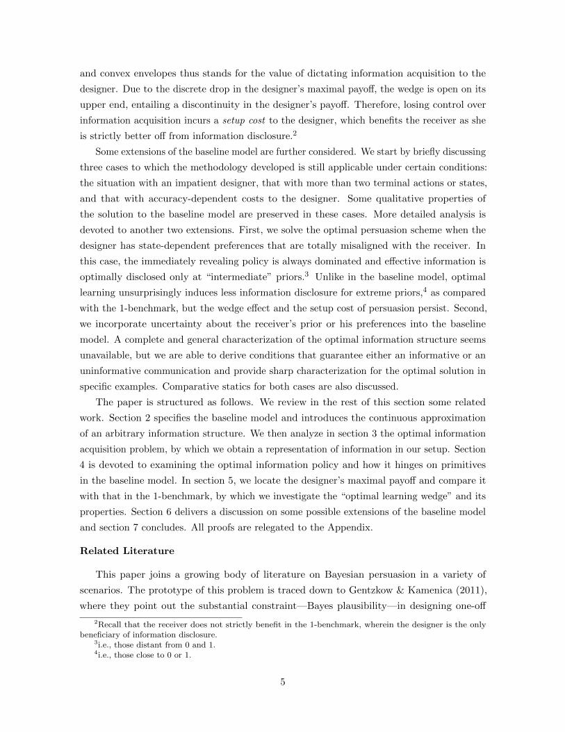
and convex envelopes thus stands for the value of dictating information acquisition to the
designer. Due to the discrete drop in the designer’s maximal payoff, the wedge is open on its
upper end, entailing a discontinuity in the designer’s payoff. Therefore, losing control over
information acquisition incurs a setup cost to the designer, which benefits the receiver as she
is strictly better off from information disclosure.2
Some extensions of the baseline model are further considered. We start by briefly discussing
three cases to which the methodology developed is still applicable under certain conditions:
the situation with an impatient designer, that with more than two terminal actions or states,
and that with accuracy-dependent costs to the designer. Some qualitative properties of
the solution to the baseline model are preserved in these cases. More detailed analysis is
devoted to another two extensions. First, we solve the optimal persuasion scheme when the
designer has state-dependent preferences that are totally misaligned with the receiver. In
this case, the immediately revealing policy is always dominated and effective information is
optimally disclosed only at “intermediate” priors.3 Unlike in the baseline model, optimal
learning unsurprisingly induces less information disclosure for extreme priors,4 as compared
with the 1-benchmark, but the wedge effect and the setup cost of persuasion persist. Second,
we incorporate uncertainty about the receiver’s prior or his preferences into the baseline
model. A complete and general characterization of the optimal information structure seems
unavailable, but we are able to derive conditions that guarantee either an informative or an
uninformative communication and provide sharp characterization for the optimal solution in
specific examples. Comparative statics for both cases are also discussed.
The paper is structured as follows. We review in the rest of this section some related
work. Section 2 specifies the baseline model and introduces the continuous approximation
of an arbitrary information structure. We then analyze in section 3 the optimal information
acquisition problem, by which we obtain a representation of information in our setup. Section
4 is devoted to examining the optimal information policy and how it hinges on primitives
in the baseline model. In section 5, we locate the designer’s maximal payoff and compare it
with that in the 1-benchmark, by which we investigate the “optimal learning wedge” and its
properties. Section 6 delivers a discussion on some possible extensions of the baseline model
and section 7 concludes. All proofs are relegated to the Appendix.
Related Literature
This paper joins a growing body of literature on Bayesian persuasion in a variety of
scenarios. The prototype of this problem is traced down to Gentzkow & Kamenica (2011),
where they point out the substantial constraint—Bayes plausibility—in designing one-off
2Recall that the receiver does not strictly benefit in the 1-benchmark, wherein the designer is the onlybeneficiary of information disclosure.
3i.e., those distant from 0 and 1.4i.e., those close to 0 or 1.
5
information structures, upon which they propose the method of “concavification” to pin
down the optimal persuasion mechanism. Alonso & Camara (2014) extend the benchmark by
introducing heterogeneous priors to agents and provide conditions for a designer to benefit
from information manipulation. They also consider the case in which the receiver’s prior is not
known to the designer. Wang (2012) studies the case of multiple receivers in a voting game
with uncertainties about the quality of alternatives. She characterizes the optimal information
structure and compares public persuasion with private persuasion.
Some other literature discusses information manipulation from a non-persuasion perspective
(without coping with information design). Brocas & Carrillo (2007) consider a model wherein
the information controller can stop the public information acquisition process contingently at
any time where the maximum number of random draws is fixed ex-ante. They characterize the
“rents” caused by the power of information controlling. A closely related, but more complex
situation appears in Lizzeri & Yariv (2010), where information manipulation happens in the
deliberation stage; before the final vote, agents should first vote on whether to go to the final
vote or to deliberate and get more information. They assume information acquisition but a
fixed and private cost is imposed on each voter. Their main conclusion is about (i) how the
length of the deliberation phase depends on the heterogeneity of committees; (ii) how the
preferences of the committees on the rules of deliberation depends on the heterogeneity of
committees; and (iii) the possibility that it is the rule of deliberation rather than the rule of
the final voting stage that determines the result.
Closer to our paper is Gill & Sgroi (2008). They consider persuading a sequence of
agents who make decisions sequentially, before which each observes a private signal about the
underlying state and the decision of the previous agent, if any, where information cascade may
happen. In their paper, the designer can only disclose a cheap signal at the very beginning,
which is observed by the first decision maker, but we have only one receiver and allow for
sequential information acquisition. Moreover, information acquisition is endogenous in our
paper, which, as will be shown, has important implications on information manipulation.
2 Model
Consider a two-agent (Designer and Receiver) game in discrete time t = 0, 1, 2, . . . . There is
a binary state ω ∈ Ω ≡ A,B, which is constant throughout the course. The agents D and
R are uncertain about ω and share an initial belief πI ∈ (0, 1) on ω = A.R’s problem is to make a single choice γ ∈ A = a, b, called his terminal decision, upon
which the game ends, to maximize his expected utility. Before making the terminal decision,
R can acquire payoff-irrelevant and conditionally independent signals about ω, one in each
time t from an information structure σt (t > 1).5 However, information acquisition delays the
5σt consists of a set of signals St 6= ∅ and two probability distributions Pt(· |A),Pt(· |B) ∈ 4St.
6

terminal decision and causes “costs” due to R’s impatience: He discounts future payoffs at a
rate r > 0. If R makes the terminal decision γ at time t in state ω, then his payoff is given by
e−rtuR(γ, ω), where
uR(γ, ω) = α1γ=a, ω=A + β1γ=b, ω=B, α, β > 0,
is his payoff before discounting. Thus, a (b, resp.) is optimal for R in state A (B, resp.) when
the true state was known. Describing R’s behavior after information acquisition is simple.
Let π ∈ [0, 1] be the posterior he has reached after learning, at which his expected payoff is
πα by choosing a and (1 − π)β otherwise. So R optimally chooses a if and only if π > π∗,
where the cutoff belief
π∗ =β
α+ β.
Thus, lying at the heart of R’s problem is the optimal termination of information acquisition,
which depends not only on π, but on the sequence of information structures σtt>0.
D is a patient persuader whose payoff relies solely on R’s terminal decision. For simplicity,
D’s preferences are given by the utility function uD(γ, ω) = 1γ=a, which is state and time-
independent. D controls information about ω as a means to affect R’s terminal decision, by
which she maximizes her expected utility—the probability that R ends up with action a.
Specifically, D selects an information structure σ in time 0 and commits to it thereafter, that
is, σt = σ for all t > 1. Therefore, R observes a sequence of conditionally i.i.d. signals from σ
about ω, and his posterior on ω = A in period T , given that σ = (S, P(s |ω)s∈S,ω∈Ω), is
πT =
πI , if T ∈ [0, 1)
πI∏bT cτ=1 P(sτ |A)
πI∏bT cτ=1 P(sτ |A) + (1− πI)
∏bT cτ=1 P(sτ |B)
, if T > 1
where S 6= ∅ is the finite set of signals and sτ ∈ S is the signal realized in time τ . Clearly, Dwill optimally choose an uninformative σ if πI > π∗ and so we assume πI < π∗, i.e., the prior
is disadvantageous to D, unless otherwise mentioned.
In our setup, D’s decision is static although she must take into account R’s dynamic
incentive for information acquisition. An alternative setup for information manipulation is
to allow σt to vary in calendar time and R’s posteriors, which then renders the scenario
a dynamic persuasion game.6 However, as long as ω is constant and the prior is common
(as we assumed), this setup does not really go beyond the 1-benchmark: D can achieve her
optimum by disclosing information essentially once, since every Bayes plausible distribution
of stopping posteriors can be attained via a signal in period 1 together with uninformative
6For dynamic Bayesian persuasion games, see, for instance, Ely (2017).
7

signals thereafter.7
2.1 Continuous Approximation
To achieve a sufficient and tractable characterization of R’s optimal information acquisition
strategy, we introduce a continuous-time approximation for an arbitrary belief updating
sequence. This is done by “collapsing” each lump-sum Bayesian updating into a process
of “gradual” learning over a unit of time. Formally, assume that a signal is drawn at each
τ ∈ ∆, 2∆, . . . for some fixed ∆ > 0 and information structure σ = (S, P(s |ω)s∈S,ω∈Ω).
The information structure associated ∆, σ∆ = (S, P∆(s |ω)s∈S,ω∈Ω), satisfies
P∆(s |ω) = D(s) + [P(s |ω)−D(s)]√
∆, for each s ∈ S, ω ∈ Ω, (2.1)
where D(s)s∈S is a state-independent distribution on S in the interior of 4S (i.e., D(s) > 0
for every s ∈ S). Clearly, we have P1(s |ω) = P(s |ω) and P∆(s |ω) → D(s) as ∆ → 0. In
other words, the two states become asymptotically indistinguishable as ∆ converges to 0, and
the information borne by a single signal decays as the sampling frequency diverges. Moreover,
as we will see later, the corresponding limit distribution of belief updating will hinge on
the choice of D(s)s∈S , and so we include D(s)s∈S as one component of an information
structure σ that D can choose henceforth.
For an interpretation, we may think of an experiment that takes time to conduct, and its
“reliability” depends on the time exerted. As sampling becomes frequent, each single signal
becomes noisier, but the experimenter is compensated by more observations in a unit time.
So the approximation (2.1), in a sense, leads to neither a gain nor a loss in informativeness as
∆ shrinks, whereby a meaningful approximation for the posterior martingale can be obtained.
To this end, we start with the law of motion of πt for a given information structure and a
fixed frequency of sampling and derive the evolution of the corresponding log-likelihood ratio.
Then, by passing ∆→ 0 and employing Ito’s lemma, we obtain the law of motion of πt in the
limit. The result is presented in Lemma 1.
Lemma 1. For an arbitrary information structure σ = (S, P(s |ω),D(s)s∈S,ω∈Ω) with
|S| < ∞ and D(s)s∈S ∈ int4S, the dynamics of posterior associated with continuous
sampling from the information structure, as approximated by (2.1), is
dπt = πt(1− πt)I(σ) dBt, (2.2)
7However, due to impatience, the optimal persuasion scheme must be more valuable to R than theconcavification solution, as the latter does not make R strictly better off and so fails to trigger learning.
8
where Bt is the standard Brownian motion, and the function I(·) is surjective, where
I(σ) =
∑s∈S
[P(s |B)−P(s |A)]2
D(s)
1/2
∈ R+ (2.3)
The posterior process πtt>0 in the continuous limit is a martingale driven by a rescaled
Brownian motion. The function I(σ) encapsulates the role σ plays in belief updating and
measures the informational accuracy of σ in the continuous-time limit: A greater I(σ)
generates more “decentralized” posteriors and hence more efficient belief updating. As
mentioned before, we can observe from (2.3) that I(σ) hinges on D(s)s∈S ; moreover, I(σ)
can achieve at most [D(s1)]−1 + [D(s2)]−1 for a given D(s)s∈S , where S ≡ s1, · · · , sn and
D(s1) 6 D(s2) 6 · · · 6 D(sn). Therefore, to reach some given level of accuracy, some D(s)
must be sufficiently low. In other words, the information loss on signal s due to continuous-time
approximation can be arbitrarily slow if the “uninformative factor” D(s) is sufficiently close
to 0. So an immediately revealing information structure is obtained, asymptotically, by an
information structure satisfying D(s)→ 0 and P(s |B) 6= P(s |A) for some s ∈ S. In addition,
each nonnegative number corresponds to an equivalent class of information structures that
have the same informational accuracy in the limit. For this reason, we use µ > 0 to represent
a typical class of equivalent information structures hereafter.
3 Information Representation
In the model, R decides when to stop the stochastic process of posteriors to balance infor-
mational gains and holdup costs. In this section, we characterize R’s optimal information
acquisition scheme under the continuous-time approximation of his belief updating process,
which will be used to represent information later on.
The strategy of R is a choice of a stopping time, and then a choice of an action in A to
maximize his expected payoff. If R chooses to stop at some π′, his decision γ ∈ A should
maximize the expected utility π′α1γ=a+(1−π′)β1γ=b. Thus, being offered an information
structure with accuracy µ, R’s problem is formulated as
maxτ∈T
E[e−rτJ(πτ ;α, β)]
s.t. dπt = πt(1− πt)µdBt
(3.1)
where T ≡ τ |E[τ ] < ∞ denotes the set of almost surely finite stopping times and the
function J : (π;α, β) ∈ [0, 1]×R2++ 7→ maxαπ, β(1− π) ∈ R+.
Let V : [0, 1]→ R be R’s optimal value function, which is assumed to be twice differen-
tiable. Since R can choose to stop at each belief π ∈ [0, 1], we must have V (π) > J(π) ≡maxαπ, β(1−π) > 0. Moreover, V is convex (see Lemma 2). These two properties, together
9

with the fact that V (0) = J(0) = β and V (1) = J(1) = α, imply that V = J on [0, L] ∪ [H, 1]
and V > J on (L,H), where L ≡ sup06π6π∗π |V (π) = J(π), called the lower stopping
posterior, and H ≡ infπ∗6π61π |V (π) = J(π), called the higher stopping posterior. Thus,
R’s optimal stopping time is τ = inft > 0 |πt /∈ (L,H), and his optimal strategy is fully
characterized by the stopping posteriors H and L, at which he is either sufficiently convinced
(at H) or unconvinced (at L) that the true state is A. He thus ends up with action a at H
and b at L, respectively.
For a sharper characterization, we denote by κ : R+ × [0, 1]→ [0, 1] a behavior (stopping)
strategy of R at every moment of time t with belief π ∈ [0, 1]. The optimal strategy κ∗ must
solve the HJB equation
rV (π) = maxκ∈[0,1]
rκJ(π) + (1− κ)[π(1− π)]2µ2V
′′(π)
2
.
Clearly, the optimal decision is the cutoff strategy κ∗ = 12rµ−2J(π)>[π(1−π)]2V ′′(π). Since
κ∗ = 0 on (L,H), the value function V satisfies the second-order differential equation
2rµ−2V (π) = [π(1− π)]2V ′′(π), ∀π ∈ (L,H). (3.2)
Plainly, the functions V and J must contact smoothly at L and H, that is, we have both
V ′(L) = −β and V ′(H) = α. The following proposition summarizes our discussion above.
Lemma 2. The value function V possesses the properties below:
(i) V (π) > J(π) = maxαπ, β(1− π) for all π ∈ [0, 1], and in particular, V (0) = J(0) = β,
V (1) = J(1) = α;
(ii) V is convex on [0, 1];
(iii) The stopping time τ = inft > 0 |πt /∈ (L,H) solves R’s optimal learning problem.
(iv) For all π ∈ [0, L] ∪ [H, 1], V (π) = J(π), where L = sup06π6π∗π | J(π) = V (π) and
H = infπ∗6π61π | J(π) = V (π). In particular, V (L) = J(L), V (H) = J(H);
(v) J ′(H) = V ′(H) = α and J ′(L) = V ′(L) = −β;
(vi) On (L,H), V solves (3.2) subject to the boundary conditions in (iv) and (v). Besides, V
is increasing in the informational accuracy µ.
The general solution to (3.2) is given by
V (π;C1, C2) = λ−1 [π(1− π)]12
(1−λ)[C1(1− π)λ + C2π
λ], (3.3)
where the parameter
λ ≡√
1 + 8rµ−2 > 1,
10

and C1, C2 are constants to be determined by boundary conditions. Note that λ ↓ 1 when the
information structure becomes immediately revealing (µ→ +∞), while λ ↑ +∞ if σ becomes
(asymptotically) uninformative (µ→ 0+). The value matching and smooth-pasting conditions
prescribed by Lemma 2 yield a closed-form expressions for L and H:
H =1
1 + αβ
(λ−1λ+1
)1/λ , L =1
1 + αβ
(λ+1λ−1
)1/λ , (3.4)
from which we obtain a relation between L and H:
H(L) =β2(1− L)
β2 + L(α2 − β2)=
1− L1 +
(α2
β2 − 1)L. (3.5)
The information structure ties together the stopping posteriors via optimal learning, contrasting
to the 1-benchmark wherein the only constraint is Bayes plausibility. Thus, (3.5) is the incentive
compatibility constraint in our context, which defines H as a function of L. Different points
on the curve H(L) correspond to different classes of information structures. Some useful
properties of this curve are presented in Lemma 3 below.
Lemma 3. (i) The function H = H(L), as defined in (3.5), is concave (resp. convex) if
and only if α 6 β (resp. α > β), and so H(L) is either concave or convex. Moreover, H
is strictly decreasing in L, and the point (π∗, π∗) is the on the graph of H(L).
(ii) H (resp. L) is strictly decreasing (resp. increasing) in λ, which implies that H (resp. L)
is strictly increasing (resp. decreasing) with the informational accuracy, and is strictly
decreasing (increasing) with impatience. Meanwhile, H and L are both strictly decreasing
with stakes ratio α/β.
(iii) limλ→1H = 1, limλ→1 L = 0; limλ→∞H = limλ→∞ L = π∗.
Lemma 3 (i) reveals the pattern of R’s best response against information quality, and
hence constitutes a representation of information in our framework. As µ increases, the two
thresholds shift apart, and the scale of change is unambiguously determined by the stakes
ratio α/β: H changes more significantly if and only if α/β > 1. (ii) says that information
quality and impatience are “symmetric” factors as they make R either “uniformly” more
cautious or “uniformly” less cautious on all actions, which implies that all pairs of posteriors
satisfying (3.5) can be ranked according to second-order stochastic dominance, and pairs of
posteriors more spreading out correspond to higher levels of µ. However, the stakes ratio plays
an “asymmetric” role: As α/β increases, R will take action a at a lower level of convincement
on state A, yet a higher level of convincement on state B is required to induce action b.
(iii) describes two extreme cases: Uninformative signals lead to immediate stopping, while
immediately revealing signals make R extremely picky.
11

4 Optimal Persuasion
Given the information representation, we move on to optimal information design. To trigger
R’s information acquisition, the information structure must feature L 6 πI . The rest discussion
will be restricted to this case, which is called effective persuasion thereafter.8 We denote by
p ∈ [0, 1] the probability that R ends up with posterior H (and hence takes action a). Given
the prior πI ∈ (0, π∗), in any effective persuasion, the optional sampling theorem prescribes
that the two posteriors must average back to the prior, and so
p =πI − LH − L
.
Geometrically, p is the fraction of segment [L, πI ] in segment [L,H]. That is, if one threshold
is relatively farther away from the prior than the other, then more likely R will hit the other
threshold. Clearly, (L,H) is Bayes plausible, but due to R’s incentive compatibility, it is
impossible to target on L and H separately, and D can only effectively choose one of the two
posteriors. Therefore, incentive compatibility confines D’s optimization in a subset of Bayes
plausible distributions and disqualify in general the concavification solution. For this reason,
we call (3.5) constrained Bayes plausibility.
A patient D maximizes p via controlling the accuracy of signals, subject to constrained
Bayes plausibility and the requirement of effective persuasion. To solve this problem, it is
more convenient to work with the lower stopping posterior L (recall that by Lemma 3 each
lower stopping posterior uniquely determines a class of equivalent information structures).
Given 0 < πI < π∗, D’s problem is formulated as
supLp =
πI − LH − L
s.t. H =β2(1− L)
β2 + L(α2 − β2), 0 6 L 6 πI
(4.1)
The solution to (4.1) is illustrated geometrically in Figure 1, wherein we graph H(L) and plot
two points, (πI , πI) and (π∗, π∗) (the latter is on the graph of H(L), according to Lemma 3),
in an LOH coordinate system. Then, consider the slope of the segment joining an arbitrary
point (L,H) on the graph of H(L) such that L 6 πI , and the point (πI , πI). Denote this
slope by k and we obtain via simple algebra that
p =1
1− k.
So D’s problem is to choose a point (L,H) on the graph of H(L) such that L 6 πI to maximize
8The restriction is inocuous to D’s optimal design problem as L > πI is never optimal for her. We maintainthis restriction here for expositional convenience.
12

the slope of the segment joining (L,H) and (πI , πI). This gives a full characterization of the
optimal persuasion policy in the baseline model.
Theorem 1 (Optimal Persuasion Policy). Given 0 < πI < π∗,
(i) it is optimal for D to be immediately revealing if and only if 0 < πI 6 π, where
π ≡ β2
α2 + β2.
In particular, immediately revealing is optimal if α 6 β;
(ii) D will optimally manipulate information if and only if π < πI < π∗; and the optimal
lower stopping posterior
L∗ =β2(α2 − β2)(1− πI)−
(α2 − β2)α2β2[π2
I (β2 − α2) + β2(1− 2πI)]
1/2
(α2 − β2)[β2 + πI(α2 − β2)].
0
1
145
π∗
(L,H)
πI
−k
H(L)
L
H
Figure 1: Geometrical characterization of optimal information structure
According to Theorem 1 (i), D can do no better than disclosing all information immediately
to gamble on a success of probability πI if R features high skepticism on state A, i.e., πI 6 π,
which relies on the stakes ratio α/β . Intuitively, for one thing, to induce a “highly skeptical”
R to experiment, the informational accuracy need to be high enough; For another thing, if we
view πI − L as the “output” and H − πI the “cost” (πI is the maximum output), then D’s
problem is to minimize the average cost subject to constrained Bayes plausibility. Since the
“marginal cost” dH/d(−L) is decreasing when H(L) is concave (i.e., α 6 β, see Figure 1), the
minimal average cost is thus achieved at the left corner. The case with profitable information
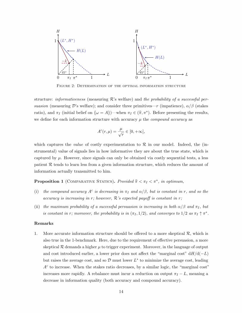
manipulation is described in Theorem 1 (ii). As shown in Figure 2 (left panel), the convexity
of H(L) alone is not enough to trigger information twist. In Figure 2 (right panel), however,
the marginal cost increases rapidly enough so that the average cost is minimized at an interior
lower posterior.
The discussion above suggests that D’s persuasion policy depends crucially on parameters.
To understand this in more detail, we focus on two perspectives of the optimal information
13
0
1
145
π∗
(L∗, H∗)
πI
−k
H(L)
L
H
0
1
145
π∗
(L∗, H∗)
πI
−k
L
H
H(L)
Figure 2: Determination of the optimal information structure
structure: informativeness (measuring R’s welfare) and the probability of a successful per-
suasion (measuring D’s welfare); and consider three primitives—r (impatience), α/β (stakes
ratio), and πI (initial belief on ω = A)—when πI ∈ (π, π∗). Before presenting the results,
we define for each information structure with accuracy µ the compound accuracy as
Ac(r, µ) =µ√r∈ [0,+∞],
which captures the value of costly experimentation to R in our model. Indeed, the (in-
strumental) value of signals lies in how informative they are about the true state, which is
captured by µ. However, since signals can only be obtained via costly sequential tests, a less
patient R tends to learn less from a given information structure, which reduces the amount of
information actually transmitted to him.
Proposition 1 (Comparative Statics). Provided π < πI < π∗, in optimum,
(i) the compound accuracy Ac is decreasing in πI and α/β, but is constant in r, and so the
accuracy is increasing in r; however, R’s expected payoff is constant in r;
(ii) the maximum probability of a successful persuasion is increasing in both α/β and πI , but
is constant in r; moreover, the probability is in (πI , 1/2), and converges to 1/2 as πI ↑ π∗.
Remarks
1. More accurate information structure should be offered to a more skeptical R, which is
also true in the 1-benchmark. Here, due to the requirement of effective persuasion, a more
skepticalR demands a higher µ to trigger experiment. Moreover, in the language of output
and cost introduced earlier, a lower prior does not affect the “marginal cost” dH/d(−L)
but raises the average cost, and so D must lower L∗ to minimize the average cost, leading
Ac to increase. When the stakes ratio decreases, by a similar logic, the “marginal cost”
increases more rapidly. A rebalance must incur a reduction on output πI − L, meaning a
decrease in information quality (both accuracy and compound accuracy).
14

2. We may think that D has some “optimal amount” of information to disclose to R via
his experimentation, which is measured by the compound accuracy. An impatient Rtends to experiment less than a more patient one. Hence, “more information” ought to
be transmitted in each moment for a less patient R, and so a more impatient R will not
be better off, although his impatience helps achieve more accurate signals, as the higher
“cost” of information acquisition also deters a “full” exploitation of those information.
3. The designer enjoys a maximum probability of a successful persuasion no lower than
πI because this is the payoff she can secure by being immediately revealing. The upper
bound, however, is due to constrained Bayes plausibility, which prescribes a minimal
amount of information necessary for triggering signal acquisition and hence brings a
setup cost to D. We view the numerical value of this upper bond, 1/2, as a consequence
of the symmetric distribution of (instantaneous) belief updating in the limit (see (2.2)).
5 The Value of Controlling Information Acquisition
In this section we examine the value of controlling information acquisition to D. In our
framework, R chooses the quantity of information via endogenous information acquisition,
while in the 1-benchmark D dictates over both the quality and the quantity of information.
Naturally, the value of controlling information acquisition is the difference between D’s
maximum payoff in the benchmark and that in our model, which will be located once we are
able to characterize D’s maximum payoff at each prior.
Concretely, let U : 4Ω → R denote D’s (expected) payoff at each of R’s stopping
posteriors. For each pair of constrained Bayes plausible stopping posteriors (L,H), denote
by `HL (·) the affine function whose graph joins the admissible pair (L,U(L)) and (H,U(H)).
Then for each prior πI < π∗, D’s maximum payoff p∗(πI) equals
max`HL (πI) | (L,H) is constrained Bayes plausible,
that is, D’s maximum value is delineated as the pointwise maximum of affine functions joining
admissible pairs, which is thus convex. We depict p∗ in Figure 3 for the case of α > β. The
constrained Bayes plausible set H(L) is graphed in the lower left quadrant, by which we find
all admissible `HL in the upper right quadrant, whose upper envelope on [0, π∗) is p∗, which is
convex and tends to 1/2 at π∗ by Proposition 1.
Now we are able to provide a geometric comparison between D’s value in the 1-benchmark
and in our model. As is well-known, D’s maximum payoff with one-shot learning is given
by the concavification solution Cav (U) (the least concave function dominating U). Figure
4 graphs D’s maximum payoff in the benchmark (denoted by Cav (U)) and in our model
(denoted by p∗). In the left panel, α 6 β, and so it is universally optimal to be immediately
15

1
1
1
145π∗
π∗
1/2p∗
H(L)
πI
p
H
L
Figure 3: The location of p∗
revealing, and so p∗ is simply the 45-degree line. In the right panel, α > β, and so on [π, π∗)
information is manipulated, p∗ being strictly convex.
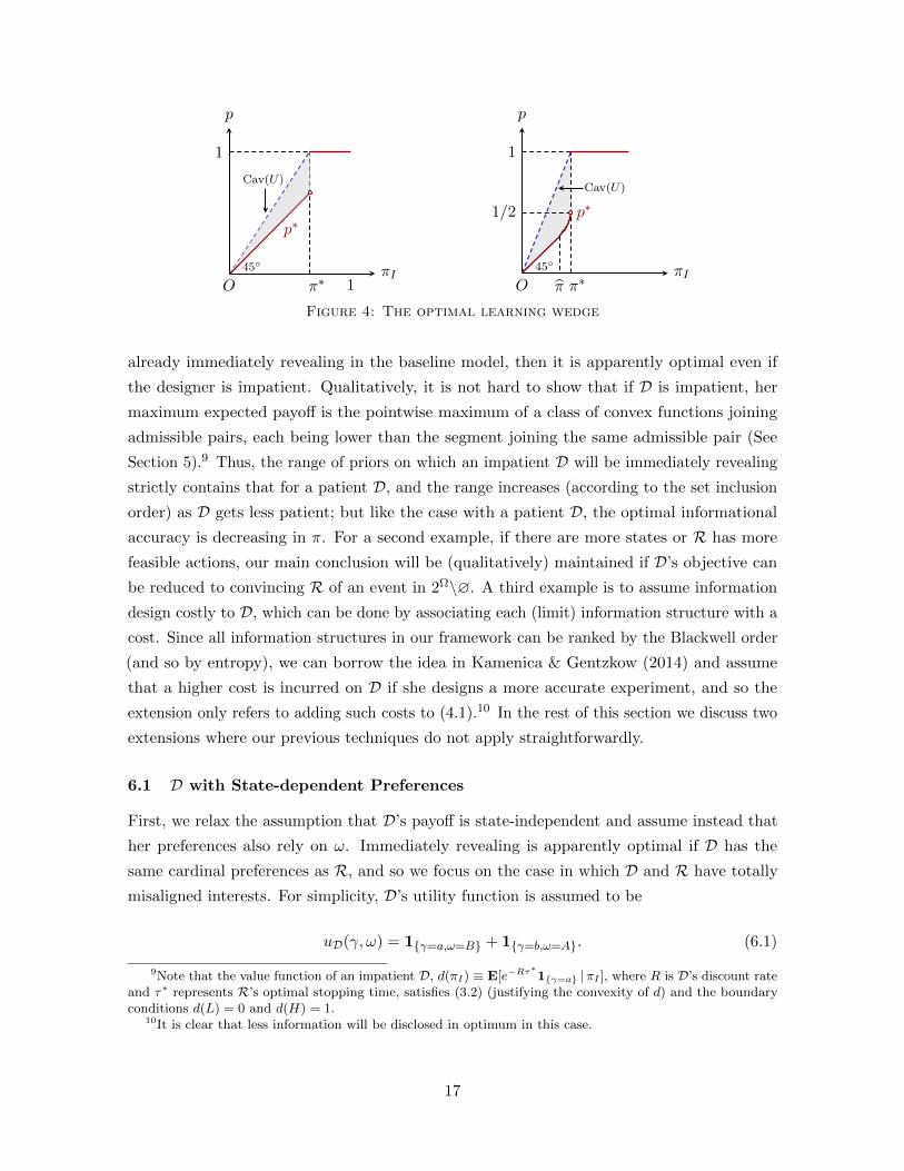
As Figure 4 illustrates, the new protocol of information transmission has down-pressed
D’s payoff, creating an “optimal learning wedge”—the convex region between Cav(U) and
p∗—as marked in gray, which represents the value of controlling information acquisition to
D. The value is everywhere positive on (0, π∗), showing that the new protocol, if thought
of as a reallocation of bargaining power in Bayesian persuasion, causes a reallocation of
benefits from additional information. In the benchmark model (see the leading example in
Gentzkow & Kamenica (2011)), R actually does not benefit from information disclosure since
at either 0 or π∗ (i.e., the two posteriors he will be sent to) action b is optimal. Therefore,
the wedge also stands to suggest a strict welfare improvement for R from optimal learning.
Moreover, the wedge has an open end on the π∗ side due to the setup cost (see Proposition 1)
to trigger effective learning, and so D’s maximum payoff exhibits a discontinuity at π∗, yet in
the benchmark model D’s payoff on both sides of π∗ can be joined seamlessly. Finally, it is
easy to see that p∗ is the lower bound of maximum payoffs to D over all scenarios of dynamic
Bayesian persuasion, wherein the dynamic information structures (in continuous limits) can
be made arbitrarily dependent on the calendar time and R’s posteriors.
6 Extensions
We have assumed in the baseline model that D is a patient persuader with state-independent
preferences, facing a situation with two states and a receiver with two terminal actions, and
the only uncertainty is about ω. Now we discuss some variations of those assumptions.
Some extensions should be forthright. For example, if the optimal information policy is
16
O
1
145
π∗
Cav(U)
p∗
πI
p
O
1
p∗
45
π∗π
Cav(U)
1/2
πI
p
Figure 4: The optimal learning wedge
already immediately revealing in the baseline model, then it is apparently optimal even if
the designer is impatient. Qualitatively, it is not hard to show that if D is impatient, her
maximum expected payoff is the pointwise maximum of a class of convex functions joining
admissible pairs, each being lower than the segment joining the same admissible pair (See
Section 5).9 Thus, the range of priors on which an impatient D will be immediately revealing
strictly contains that for a patient D, and the range increases (according to the set inclusion
order) as D gets less patient; but like the case with a patient D, the optimal informational
accuracy is decreasing in π. For a second example, if there are more states or R has more
feasible actions, our main conclusion will be (qualitatively) maintained if D’s objective can
be reduced to convincing R of an event in 2Ω\∅. A third example is to assume information
design costly to D, which can be done by associating each (limit) information structure with a
cost. Since all information structures in our framework can be ranked by the Blackwell order
(and so by entropy), we can borrow the idea in Kamenica & Gentzkow (2014) and assume
that a higher cost is incurred on D if she designs a more accurate experiment, and so the
extension only refers to adding such costs to (4.1).10 In the rest of this section we discuss two
extensions where our previous techniques do not apply straightforwardly.
6.1 D with State-dependent Preferences
First, we relax the assumption that D’s payoff is state-independent and assume instead that
her preferences also rely on ω. Immediately revealing is apparently optimal if D has the
same cardinal preferences as R, and so we focus on the case in which D and R have totally
misaligned interests. For simplicity, D’s utility function is assumed to be
uD(γ, ω) = 1γ=a,ω=B + 1γ=b,ω=A. (6.1)
9Note that the value function of an impatient D, d(πI) ≡ E[e−Rτ∗1γ=a |πI ], where R is D’s discount rate
and τ∗ represents R’s optimal stopping time, satisfies (3.2) (justifying the convexity of d) and the boundaryconditions d(L) = 0 and d(H) = 1.
10It is clear that less information will be disclosed in optimum in this case.
17

Here we drop the restriction that πI < π∗ since it is no longer a trivial decision for D when
πI > π∗. Thus, D’s expected payoff function U : 4Ω→ R is
U(π) =
π, π ∈ [0, π∗)
1− π, π ∈ [π∗, 1].
Now the objective of D is to maximize p(L)[1−H(L)] + [1− p(L)]L, where L is viewed as the
control variable and p(L) represents the probability that R ends up with the higher posterior.
Specifically, when π∗ = 1/2 (equivalently, α = β), U is concave, and so D should optimally
disclose no information. When α > β (π∗ < 1/2), U has an up-jump at π∗, meaning that
cav[U ](πI) = uD(πI) for all πI > π∗ and hence there should be no information disclosure
on [π∗, 1]; if, however, πI < π∗, then it is worth for D disclosing additional information if
and only if H(πI) 6 1/2, because an effective persuasion requires L < πI , which will never
be optimal if such an L causes H > 1/2 since otherwise D’s expected utility will be even
dominated by U(πI), the value of no information disclosure. For α < β we have a symmetric
result. The following proposition characterizes the optimal information policy.
Proposition 2. Given preferences (6.1), D will optimally be informative (i.e., µ > 0) if and
only if πI ∈ (π ∧ π∗, π ∨ π∗), and in this case the optimal lower posterior
L∗ =1− πI +
(αβ
)2(1 + πI)− α
β
[(αβ
)2 − 1] [
(1− πI)2 − π2I
(αβ
)2]1/2
1− πI +(αβ
)2 [3 + πI
(αβ
)2] .
Based on Proposition 2, we can further show that less accurate information should be
offered to a less skeptical R, while the patience of R, like before, does not affect the compound
accuracy and hence the payoff equivalence property is preserved (but a more patient R will
be provided with a less accurate information structure). Moreover, D’s expected utility is
increasing (resp. decreasing) in the stakes ratio when α > β (resp. α < β). Finally, as is
featuring our framework, there is a setup cost of persuasion at π∗, which equals 1/2 of the
maximum payoff D receives when it is optimal to be uninformative.11
6.2 Uncertainty about R
The second extension refers to introducing asymmetric information to the Baseline setup.
Specifically, we discuss some implications of asymmetric information on D’s prior and his
stakes ratio, respectively, with other setup being identical to that in the baseline model.12
11A proof for those comparative static results can be found the Appendix.12Note that D cannot get strictly better off by screening R, because D can only control the informational
accuracy while all types of R prefer more accurate signals.
18

6.2.1 Uncertainty about R’s prior
Assume that R is privately informed of his type—prior π ∈ [0, 1], which follows a (continuous)
probability density h : (0, 1) → R++, for simplicity, and D’s prior πI = Eh[π] ∈ (0, 1). An
alternative interpretation of this is that D is trying to persuade a unit mass of people whose
priors are distributed according to h, i.e., there are heterogeneous priors, possibly because
people have already acquired some information about the true state through heterogeneous
channels.
Notice that the optimal information acquisition policy does not depend on R’s prior, and
hence D knows that if she employs a persuasion scheme that induces (L,H), the probability
for R to end up with action a (treating L as the control variable), p(L), satisfies
p(L) =
ˆ H(L)
L
π − LH(L)− L
· h(π) dπ +
ˆ 1
H(L)h(π) dπ, L ∈ [0, π∗]
where H(L) is given by (3.5). Then it is immediate to see that p(0) = πI and p(π∗) =´ 1π∗ h(π) dπ. An interior optimal solution is characterized by the first-order condition
0 = p′(L) =
ˆ H
L
H ′(L− π) + (π −H)
(H − L)2h(π) dπ
=
´ HL h(π) dπ
(H − L)2(L−Eh[π |π ∈ [L,H])
(H ′ − H −Eh[π |π ∈ [L,H]]
L−Eh[π |π ∈ [L,H]]
),
based on which we have
p′(L) > 0 if and only if H ′ 6H −Eh[π |π ∈ [L,H]]
L−Eh[π |π ∈ [L,H]]≡ Rh(L), (6.2)
where Rh(π∗) ≡ limL↑π∗ Rh(π). In general, Rh(L) and Eh[π |π ∈ [L,H]] can be non-monotonic
so that H ′ and Rh may cross multiple times. However, some useful information about the
optimal disclosure policy can still be extracted. As a simple example, the optimal persuasion
mechanism is immediately revealing if Supph ⊆ (0, π∗) ⊆ (0, π) since by Theorem 1 it is now
optimal to be immediately revealing to each possible type. A more involved example below
assumes a uniformly distributed prior.
Example. [Uniformly distributed prior] Assume that π ∼ U [0, 1]. Then we have Rh(L) = −1
for all L ∈ [0, π∗]. Thus, when α > β, one can check that H ′ 6 Rh(L) for all L ∈ [0, π∗], and
hence by (6.2) it is optimal to be uninformative (i.e., µ = 0); when α < β, however, we will
have H ′ > Rh(L) on [0, π∗], which means that it is optimal to be immediately revealing. It
suggests that evenly distributed opinions, given homogeneity of stakes ratio, essentially cause
either immediate disclosure or no disclosure of information in our framework.
More generally, we present in Proposition 3 two sufficient conditions that guarantee
19
information manipulation and informative persuasion, respectively.
Proposition 3. The optimal lower stopping posterior L∗ > 0 (i.e., not immediately revealing)
if Eh[π] > π; and L∗ < π∗ (i.e., not totally uninformative) if h(π∗) > 0 and h′(π∗)h(π∗) <
3(β2−α2)αβ .
How do the compound accuracy and the probability of a successful persuasion hinge on
primitives in optimum? Although it is clear that both are independent to R’s impatience,
one might be tempted to guess, according to Proposition 1, that the optimal information
structure becomes less accurate as Eh[π] increases. However, stronger conditions are needed
to guarantee a higher level of accuracy. Also, it may not be true that the compound accuracy
is decreasing in the stakes ratio α/β for two reasons: First, the optimal lower threshold, when
uncertainty about π is present, may not satisfy the tangent condition for each type, and so
for low types a lower L would yield higher probability of successful persuasion;13 Second,
increasing the accuracy could be profitable since some types lower than L would then get
involved in experimentation rather than making terminal decisions immediately. The main
result is presented below.
Proposition 4. With uncertainties in D’s prior being given by h : (0, 1)→ R++,
(i) the optimal compound accuracy decreases if h is replaced by h such that h(π)/h(π) is
increasing in π;
(ii) the probability of a successful persuasion increases when h is replaced by h such that h
first-order stochastically dominates h, or when the stakes ratio increases.
6.2.2 Uncertainty about the stakes ratio
Now the prior πI ∈ (0, 1) is common knowledge again but the stakes ratio x ≡ α/β is R’s
private information, which, as D believes, has a smooth density ϕ : [ξ, ξ] → R++, where
ξ, ξ > 0. ϕ generates a distribution over the lower stopping posteriors L(z;x) for each
z ≡(λ+1λ−1
)1/λ ∈ [1,∞],14 which is chosen by D. A greater value of z means more accurate
information structure. Then, by (3.4), the probability of a successful persuasion at z can be
written as
p(z) =
ˆ ξ
ξP (z;x)ϕ(x) dx,
13More precisely, for types π such that π < H−LH′(L)1−H′(L)
, given L.14By Lemma 3, dz/dλ < 0, limλ→1 z =∞, and limλ→∞ z = 1.
20
where the probability of successfully persuading a type x receiver by a z-parameterized
information structure
P (z;x) =
0, if x 6 x(z)
πI − L(z;x)
H(L(z;x))− L(z;x), if x(z) < x 6 x(z)
1, if x > x(z).
,
x(z) ≡ z(π−1I − 1) being the upper bound of stakes ratios above which the probability of a
successful persuasion is 1; x(z) ≡ z−1(π−1I − 1) being the lower bound of stakes ratios below
which the probability of a successful persuasion is 0. For x ∈ (x(z), x(z)], by (3.4), we have
P (z;x) =1
z2 − 1
[πIz
2 +
(πI − 1 + πIx
2
x
)z + (πI − 1)
]. (6.3)
The extreme values of p(z) are p(∞) = πI and p(1) =´ ξπ−1I −1
ϕ(x) dx. Then it is easy to see
that an interior solution z∗ is characterized by
ˆ x(z∗)
x(z∗)
∂P
∂z(z∗;x)ϕ(x) dx = 0.
Here, except for some special cases (for example, if πI 6 infmin 1x2+1
, 1x+1 |x ∈ suppϕ,
then it is optimal to be immediately revealing, since for each possible type the best strategy
for D is to do so), a neat characterization seems not achievable due to the fully nonlinear
structure and the underspecification of ϕ. However, some comparative statics can still be
derived indirectly.
Proposition 5. If α/β is distributed according to ϕ : [ξ, ξ]→ R++, then
(i) the optimal compound accuracy decreases if ϕ is replaced by ϕ such that ϕ(x)/ϕ(x) is
increasing in x; and
(ii) the probability of successful persuasion increases if people have a higher prior on ω = A,or if ϕ is replaced by ϕ which first-order stochastically dominates ϕ.
7 Concluding Remarks
We study in this paper strategic information transmission with committed signals in a protocol
that the receiver optimally acquires signals from the information channel offered by the designer.
Adopting a belief-based approach, we propose a tractable continuous-time approximation for
dynamic belief updating and obtain a convenient geometric representation of information.
Based on this, we fully characterize the optimal persuasion scheme and examine how the
21

welfare from additional information is reallocated between the two agents. It is optimal to be
immediately revealing for low prior or low stakes ratio, while in the other cases the space of
information manipulation is significantly limited due to the receiver’s optimal learning. The
discrete drop in the designer’s expected payoff reveals a setup cost of information transmission
and yields a wedge that measures the value of controlling information quantity in Bayesian
persuasion. Some extensions of the baseline model are also discussed. Overall, the new
protocol results in an endogenous refinement of Bayes plausible signals and new techniques to
pin down the optimal information structure. The results speak to how incentives in Bayesian
persuasion are reshaped when the receiver actively chooses the extent to which he would like
to be persuaded by costly signals, and more broadly, to literature on dynamic sender-receiver
games.
A number of potentially interesting research problems stem from our analysis so far.
First, we may consider the implications of some exogenously fixed deadline for information
acquisition when information manipulation is profitable (for instance, in some online sales
platform, consumers are offered a certain length of time for free trial), where the major
challenge is to characterize how the stopping posteriors are distributed at that deadline.
Second, as mentioned earlier in section 2, we can view our setup as a special case in a more
general class of dynamic Bayesian persuasion games, wherein there is some effective restriction
on sequential informativeness, and so different versions of the restriction may yield different
predictions. The restriction considered in our setup is that all sequential signals have to have
the same accuracy, and the most straightforward extension is to allow the accuracy to (weakly)
increase, depending on R’s posteriors and/or the calendar time.15 A dual extension of this
is to allow the accuracy to vary freely over time and history but to have either a changing
state or uncertainty about R (for example, his prior or stakes ratio). Finally, the situation
with an impatient designer might deserve some further attention. We have not obtained a
complete characterization for the optimal information structure for this case. To figure out
the optimal solution and answer questions like whether a less patient D will provide more
information, the key is to determine how D’s value function d(πI) (see footnote 9) depends
on informational accuracy, but the answer is not obvious; the optimal stopping time could be
short when the accuracy is either sufficiently high or sufficiently low. Although a closed form
solution for d(πI) at each given admissible pair can be obtained via the differential equation
and boundary conditions given in footnote 9, the solution does not seem easy to employ for
our purpose; some new approaches are needed, which we will leave for future research.
15For an interpretation, R can request D conduct multiple rounds of investigation, but additional investiga-tions have to be “better” or “more informative” than those already done.
22

8 Appendix
8.1 Proof of Lemma 1
Let the signal space S = s1, s2, . . . , sn. We start with a given frequency ∆−1 of sampling and some t > 0 at
which R possesses a belief πt ∈ (0, 1) on ω = A. For each s > t, according to Bayes’ rule, the stochastic
posterior πs, by (2.1), satisfies (assuming ∆ < mins− t, 1)
ln1− πsπs
= ln1− πtπt
+
b s−t∆ c∑τ=1
lnD(sτ ) + [P(sτ |B)−D(sτ )]
√∆
D(sτ ) + [P(sτ |A)−D(sτ )]√
∆. (8.1)
For notational convenience, we denote for each τ the log-likelihood ratio by LLR∆(sτ ), that is,
LLR∆(sτ ) ≡ lnD(sτ ) + [P(sτ |B)−D(sτ )]
√∆
D(sτ ) + [P(sτ |A)−D(sτ )]√
∆
= ln
(1 +
δ(sτ )√
∆
D(sτ ) + [P(sτ |A)−D(sτ )]√
∆
), (8.2)
where δ(si) ≡ P(si |B)−P(si |A) ∈ [−1, 1], i ∈ 1, 2, . . . , n. Then, if measured by information up to t, the
probability that LLR∆(sτ ) = LLR∆(sj), denoted by P∆(si), satisfies16
P∆(si) = πtP∆(si |A) + (1− πt)P∆(si |B) = D(si) + q(si)
√∆,
where q(si) ≡ P(si |B)− πtδ(si)−D(si), i = 1, 2, . . . , n. Meanwhile, by (8.1), the log-probability ratio ln 1−πsπs
,
as measured by information up to t, is the sum of a constant and a (finite) sequence of i.i.d. random variables.
Therefore, when ∆ is small, the central limit theorem implies that
ln 1−πsπs− ln 1−πt
πt− s−t
∆E∆(LLR |πt)√
s−t∆
Var∆(LLR |πt)⇒ N (0, 1),
where E∆(LLR |πt) (resp. Var∆(LLR |πt)) is the conditional expectation (resp. variance) of the log-likelihood
ratio associated with the information structure with the sampling frequency ∆−1. As a result, we have
ln1− πsπs
− ln1− πtπt
⇒ N(
(s− t) lim∆→0+
E∆(LLR |πt)∆
, (s− t) lim∆→0+
Var∆(LLR |πt)∆
)
= lim∆→0+
E∆(LLR |πt)∆
(s− t)−
√lim
∆→0+
Var∆(LLR |πt)∆
(Bs −Bt), (8.3)
B representing the standard Brownian motion. To proceed, we first argue that
lim∆→0+
E∆(LLR |πt)∆
=1− 2πt
2
n∑i=1
δ2(si)
D(si), lim
∆→0+
Var∆(LLR |πt)∆
=
n∑i=1
δ2(si)
D(si).
To this end, we will show that E∆(LLR) = O(∆) and Var∆(LLR) = O(∆), as well as compute the limits
lim∆→0+1∆E∆(LLR) and lim∆→0+
1∆
Var∆(LLR). By definition,
E∆(LLR) =
n∑i=1
[D(si) + q(si)
√∆]
lnD(si) +
[P(si |B)−D(si)
]√∆
D(si) + [P(si |A)−D(si)]√
∆.
16For our purpose, it is without loss of generality to require that LLR∆(si) 6= LLR∆(sj) for all 1 6 i < j 6 n,and hence the distribution is well-defined.
23

Letting x ≡√
∆, then E∆(LLR) is smooth on [0, 1), and by Taylor’s theorem,
E∆(LLR) = E∆(LLR)x=0 +dE∆(LLR)
dx
∣∣∣∣x=0
x+d2E∆(LLR)
2dx2
∣∣∣∣x=0
x2 +O(x3).
Moreover, it is straightforward to derive that E∆(LLR)x=0 = 0,
dE∆(LLR)
dx
∣∣∣∣x=0
=
n∑i=1
q(si) ln
D(si) + [P(si |B)−D(si)]x
D(si) + [P(si |A)−D(si)]x+
[D(si) + q(si)x
]D(si)δ(si)∏
ω=A,B D(si) + [P(si |ω)−D(si)]x
x=0
=
n∑i=1
δ(si) = 0,
and
d2E∆(LLR)
dx2
∣∣∣∣x=0
=
n∑i=1
q(si)D(si)δ(si)∏
ω=A,B D(si) + [P(si |ω)−D(si)]x +q(si)D(si)δ(si)∏
ω=A,B D(si) + [P(si |ω)−D(si)]x−
D3(si)δ(si)[P(si |B) + P(si |A)− 2D(si)
]∏ω=A,B D(si) + [P(si |ω)−D(si)]x2
+ o(x)
x=0
=
n∑i=1
δ(si)[2q(si)−P(si |A)−P(si |B) + 2D(si)
]D(si)
=
n∑i=1
δ(si)[2P(si |B)− 2πtδ(s
i)− 2D(si)−P(si |A)−P(si |B) + 2D(si)]
D(si)
=
n∑i=1
(1− 2πt)δ2(si)
D(si).
Therefore,
lim∆→0+
E∆(LLR)
∆= limx→0+
E∆(LLR)
x2=
d2E∆(LLR)
2dx2
∣∣∣∣x=0
=
n∑i=1
(1− 2πt)δ2(si)
2D(si).
Also, since
limx→0+
1
xlnD(si) +
[P(si |B)−D(si)
]x
D(si) + [P(si |A)−D(si)]x= limx→0
D(si)δ(si)∏ω=A,B D(si) + [P(si |ω)−D(si)]x =
δ(si)
D(si), (8.4)
we know that
lnD(si) +
[P(si |B)−D(si)
]√∆
D(si) + [P(si |A)−D(si)]√
∆= O
(√∆).
Then by definition,
Var∆(LLR) =
n∑i=1
[D(si) + q(si)
√∆]
lnD(si) +
[P(si |B)−D(si)
]√∆
D(si) + [P(si |A)−D(si)]√
∆−E∆(LLR)
2
=
n∑i=1
D(si)
lnD(si) +
[P(si |B)−D(si)
]√∆
D(si) + [P(si |A)−D(si)]√
∆
2
+ o(∆),
which means that (using (8.4))
lim∆→0+
Var∆(LLR)
∆=
n∑i=1
D(si)δ2(si)
D2(si)=
n∑i=1
δ2(si)
D(si).
24

With the result above, we let s = t+ dt in (8.3) and arrive at
d
(ln
1− πtπt
)=
[1− 2πt
2
n∑i=1
δ2(si)
D(si)
]dt−
(n∑i=1
δ2(si)
D(si)
)1/2
dBt. (8.5)
Define f(x) = (1 + ex)−1 (x ∈ R). Clearly, f is infinitely differentiable and it is easy to obtain that
df
dx=
−ex
(1 + ex)2,
d2f
dx2=ex(e2x − 1)
(ex + 1)4.
Since
f
(ln
1− πtπt
)= πt,
we can use Ito’s lemma to (8.5) and get
dπt =
1− 2πt
2
[n∑i=1
δ2(si)
D(si)
]− 1−πt
πt(1−πtπt
+ 1)2 +
1
2
[n∑i=1
δ2(si)
D(si)
]1−πtπt
[(1−πtπt
)2 − 1](
1−πtπt
+ 1)4
dt
+
[n∑i=1
δ2(si)
D(si)
]1/2(1− πt)/πt(1−πtπt
+ 1)2 dBt
= πt(1− πt)
[n∑i=1
δ2(si)
D(si)
]1/2
dBt
= πt(1− πt)I(σ) dBt.
Finally, we prove that the mapping I, as defined in (2.3), is surjective. Pick an arbitrary x ∈ R+. It
is clear that x = 0 can be achieved by any information structure with S being a singleton. If x 6= 0, then
consider an information structure σ = (P(s |ω),D(s)s∈S,ω∈Ω) such that S = s1, s2. It is easy to check
that every x ∈ (0, 2) can be achieved by setting D(s1) = 1/2 and P(s1 |A) = P(s2 |B) = 12(1 + x/2), while
every x ∈ [2,+∞) can be achieved by setting P(s1 |A) = P(s2 |B) = 1 and D(s1) = 12(1 +
√1− 4/x2). This
concludes our proof for Lemma 1.
8.2 Proof of Lemma 2
Properties (ii) and (vi) remain to be established. For (ii), note that a function W satisfying (3.2) is convex
since W ′′(π) > 0 by that equation. Therefore, as the value function V (π) = maxW (π), J(π) for some W
solving (3.2) while J is convex, V must be convex.
For (vi), suppose for µ′ > µ, the corresponding pairs of optimal stopping posteriors are (L′, H ′) and (L,H),
respectively. We argue that R will get strictly better off even if he adopts the stopping strategy (H,L) at µ′.
Indeed, given the information structure characterized by µ′ and the stopping strategy (L,H), the expected
payoff to R is
Eµ′e−rτ maxαπτ , β(1− πτ )
= αH · πI − LH − L
ˆ ∞0
e−rtgµ′(t |H) dt+ β(1− L) · H − πI
H − L
ˆ ∞0
e−rtgµ′(t |L)dt,
where τ is the stopping time determined by the strategy (L,H), and g(t |$) is the conditional distribution
of the stopping time given that the posterior stops at $ ∈ L,H. To establish the desired result, we need
to show that´∞
0e−rtgµ
′(t |$) dt >
´∞0e−rtgµ(t |$) dt. First, notice that the stochastic process of posteriors
πt(µ′)t>0 is always a martingale, and hence by Dambis-Dubins-Schwarz Theorem, πt(µ′) = π∗ + BAt(µ′),
25

where BAt(µ′) is a time-changed Brownian motion, and the changed time (by (2.2)) is
At(µ′) = inf
v > 0
∣∣∣∣ ˆ v
0
1
(µ′)2(1− π∗ −Bu)2(π∗ +Bu)2du = t
. (8.6)
Fix an arbitrary trajectory of the Brownian motion B(ω). It is then easy to observe from (8.6) that for each
u > 0 we have
1
(µ′)2[1− π∗ −Bu(ω)]2[π∗ +Bu(ω)]26
1
µ2[1− π∗ −Bu(ω)]2[π∗ +Bu(ω)]2,
which then implies that At(µ′)(ω) 6 At(µ)(ω). Since ω is arbitrary, this means that Pµ′(τ > T |$) 6 Pµ(τ >
T |$) for all T > 0 and $ ∈ L,H. Therefore,
ˆ ∞0
e−rtgµ′(t |$) dt =
ˆ 1
0
[1−Pµ′(e−rt 6 y |$)] dy
=
ˆ 1
0
[1−Ps′
(t >
1
rln
1
y
∣∣∣∣$)] dy
>ˆ 1
0
[1−Pµ
(t >
1
rln
1
y
∣∣∣∣$)] dy
=
ˆ ∞0
e−rtgµ(t |$) dt,
completing the proof.
8.3 Proof of Lemma 3
For (i), it is easy to obtain that
dH
dL=
−α2β2
[β2 + (α2 − β2)L]2,
d2H
dL2=
2α2β2(α2 − β2)
[β2 + (α2 − β2)L]3.
We always have dH/dL < 0, while d2H/dL2 > 0 if and only if α > β. The last claim follows immediately if we
plug this point back to the expression of H(L), which actually represents the case of uninformative signals.
The second half of (ii) is immediate from inspecting (3.4). For the first half, shall we consider the function
f(λ) ≡(λ− 1
λ+ 1
)1/λ
= exp
1
λlnλ− 1
λ+ 1
.
Clearly, H = 11+α
βf(λ)
and L = 11+α
β[f(λ)]−1 . It is then easy to derive that
df(λ)
dλ= f(λ) ·
[1
λ2lnλ+ 1
λ− 1+
2
λ(λ2 − 1)
]> 0,
which yields the monotonicity claimed. For (iii), notice that
limλ→1
f(λ) = 0, limλ→∞
f(λ) = limλ→∞
(λ− 1
λ+ 1
)1/λ
= limλ→∞
[(1− 2
λ+ 1
)−λ+12] −2λ(λ+1)
= 1,
which, appended to (3.4), gives us the desired result.
26

8.4 Deriviation of equation (3.5)
Note that the value-matching and smooth-pasting conditions at L and H prescribe the the following system
about (L,H;C1, C2):
C1(1− L)λ + C2Lλ =
(1− L)λβ
[L(1− L)]12
(1−λ)(8.7)
C1(1−H)λ + C2Hλ =
λHα
[H(1−H)]12
(1−λ)(8.8)
C1(1− L)λ(1− λ− 2L) + C2Lλ(1 + λ− 2L) =
−2λβ
[L(1− L)]12
(1−λ)−1(8.9)
C1(1−H)λ(1− λ− 2H) + C2Hλ(1 + λ− 2H) =
2λα
[H(1−H)]12
(1−λ)−1(8.10)
From (8.8) we solve
C2Hλ =
λHα
[H(1−H)]12
(1−λ)− C1(1−H)λ. (8.11)
Appending (8.11) to (8.10), we arrive atλHα
[H(1−H)]12
(1−λ)− C1(1−H)λ
(1 + λ− 2H) + C1(1−H)λ(1− λ− 2H) =
2λα
[H(1−H)]12
(1−λ)−1,
from which we solve
C1 =α(λ− 1)
2(
1−HH
) 12
(1+λ). (8.12)
Similarly, we can also get (from (8.7) and (8.9))
C2 =β(λ− 1)
2(
L1−L
) 12
(1+λ). (8.13)
Then, it follows immediately after our plugging (8.12) and (8.13) back to (8.7) that
α(λ− 1)(1− L)λ
2H−12
(1+λ)(1−H)12
(1+λ)+
β(λ− 1)Lλ
2L12
(1+λ)(1− L)−12
(1+λ)=
λβ(1− L)
[L(1− L)]12
(1−λ),
which can be transformed intoL
12
(1−λ)(1− L)12
(λ−1)
H−12
(1+λ)(1−H)12
(λ+1)=β(λ+ 1)
α(λ− 1). (8.14)
Similar algebra leads us to
H12
(λ−1)(1−H)12
(1−λ)
L12
(1+λ)(1− L)−12
(1+λ)=α(λ+ 1)
β(λ− 1). (8.15)
Dividing (8.15) from (8.14), we finally obtain (3.5).
8.5 Proof of Theorem 1
Here we will fully employ the geometric relations. Consider the segment ` connecting (0, 1) and (πI , πI) and it
is easy to see that the graph of H(L) is everywhere strictly higher than ` on (0, πI ] if and only if the slope
of ` is no greater (taking into account the sign) than H ′(0). Indeed, if H(L) is concave, then `(L) < H(L)
on (0, πI ]: the set C ≡ (L,H) | 0 6 L 6 1, H 6 H(L) is convex and (πI , πI) ∈ int C, which implies that
γ(0, 1) + (1− γ)(πI , πI) | 0 6 γ < 1 ⊆ int C. In this case, as α 6 β and πI < π∗ = βα+β
, it is easy to check
27

that (using the expression of H ′(L) derived in the proof of Lemma 3)
Slope(`) =1− πI−πI
< 1−(
1 +α
β
)= −α
β6 −
(α
β
)2
= H ′(0).
If H(L) is strictly convex and `(0) = H(0), then as the set C ≡ (H,L) | 0 6 L 6 πI , H > H(L) is convex
while C and ` contact at (0, 1), H(L) > `(L) on (0, πI ] if and only if ` is lower than the supporting hyperplane
of C at (0, 1) whose slope is rightly H ′(0),17 which is equivalent to Slope(`) 6 H ′(0).
For Theorem 1 (i), it suffices to show that for any (L,H(L)) such that L ∈ (0, π], H(L) > `(L), which,
according to our claim above, is equivalent to Slope(`) 6 H ′(0), that is, 1−πI−πI
6 −(αβ
)2, from which we solve
πI 6β2
α2+β2 , proving Theorem 1 (i). For the rest of (i), notice that α 6 β implies πI 6 π.
For Theorem 1 (ii), first notice that now H(L) is strictly convex (as α > β), and by Theorem 1 (i), if
πI >β2
α2+β2 , then there is a unique L ∈ (0, πI) (due to strict convexity) such that `(L) = H(L). Consider the
function
k(L) ≡ πI − LH(L)− L
for L ∈ [0, πI ]. Clearly, k(0) = k(L), which, by Intermediate Value Theorem, implies that there is some
L ∈ (0, L) such that H ′(L) = k(0). Then we deduce from the strict convexity of H(L) that H ′(L) > k(0).
Therefore, the tangent line of H(L) at L achieves a value strictly greater than πI at πI (as `(πI) = πI and
` goes through (L,H(L))). However, since H ′(0) < Slope(`) (by Theorem 1 (i)), the tangent line of H(L)
at (0, 1) achieves a value strictly less than πI at πI . By continuity, there is some L∗ ∈ (0, πI) such that
H(L∗) = H ′(L∗)(L∗ − πI) + πI , or equivalently, H ′(L∗) = πI−H(L∗)πI−L∗
. Note that such L∗ is unique since H(L)
is strictly convex. Now we claim that k is maximized at L∗, which is obvious as the tangent line of H(L) at L∗,
denoted by `∗, is the supporting hyperplane of the convex set C, which implies that all segments connecting
(πI , πI) and some point on H(L) must be above `∗. Hence, k(L) 6 H ′(L∗) for all L ∈ [0, πI ] (note that we can
define k(πI) = −∞). Finally, by what we have shown above, L∗ is characterized by the tangent condition
H ′(L∗) =−α2β2
[β2 + (α2 − β2)L∗]2=H(L∗)− πIL∗ − πI
=
β2(1−L∗)β2+(α2−β2)L∗ − πI
L∗ − πI.
Solving this equation for L∗ gives us the desired result (note that since H(L) is symmetric against the 45-line,
the equation above has two real roots, one on each side of π∗. We take the smaller one to fit the constraint
that L∗ < π∗).
8.6 Proof of Proposition 1
We first state and prove a lemma. For expositional convenience, in the following we use x to represent α/β
(and correspondingly x′ represents another stakes ratio). We assume x, x′ > 1 throughout the proof.
Lemma 4. Let L∗(x) be the optimal lower threshold for H(L;x) (and denote by H∗ the corresponding optimal
higher threshold). Then the tangent line of H(L;x′) at L∗(x) achieves a value lower than πI at πI if x′ > x.
Proof. Consider the tangent line of H(L;x) at L∗(x). First, we have
∂H(L;x)
∂x=
∂
∂x
[1− L
1 + (x2 − 1)L
]=−2xL(1− L)
[1 + (x2 − 1)L]2=−2L(1− L) · 1
x[1x
+(x− 1
x
)L]2 ,
17Here we slightly extend the domain of H(L) to (−ε, 1] for some small ε > 0 to make (0, 1) not a kinkypoint, since otherwise the subdifferential of H(L) at (0, 1) is not a singleton.
28

and∂2H(L;x)
∂x∂L=
∂
∂x
−1[
1x
+(x− 1
x
)L]2
=2[L(1 + 1
x2
)− 1
x2
][1x
+(x− 1
x
)L]3 .
Hence, by changing x marginally, the corresponding infinitesimal change of the intercept of the tangent line on
the vertical line L = π∗ is
−2L∗(x)(1− L∗(x)) · 1x[
1x
+(x− 1
x
)L∗(x)
]2 +2[L∗(x)
(1 + 1
x2
)− 1
x2
][1x
+(x− 1
x
)L∗(x)
]3 [πI − L∗(x)] , (8.16)
We are interested in determining the sign of (8.16). To this end, we transform (8.16) into
1[1x
+(x− 1
x
)L∗(x)
]3 ·2[L∗(x) + (L∗(x)− 1) · 1
x2
](πI − L∗(x))
− 2x· L∗(x)(1− L∗(x)) ·
[1x
+(x− 1
x
)L∗(x)
]︸ ︷︷ ︸
(I)
and, since x > 1, it only remains to figure out the sign of (I). By Theorem 1 (ii), we have
−α2β2
[β2 + (α2 − β2)L∗(x)]2=
β2(1−L∗(x))
β2+(α2−β2)L∗(x)− πI
L∗(x)− πI,
or equivalently,
2
x· L∗(x)(1− L∗(x))
[1
x+
(x− 1
x
)L∗(x)
]=
2πIL∗(x)
[1x
+(x− 1
x
)L∗(x)
]2+2L∗(x)(πI − L∗(x))
. (8.17)
Using (8.17) in (I), we obtain
(I) = 2
[L∗(x) + (L∗(x)− 1) · 1
x2
](πI − L∗(x))− 2
x· L∗(x)(1− L∗(x)) ·
[1
x+
(x− 1
x
)L∗(x)
]
= 2
[L∗(x) + (L∗(x)− 1) · 1
x2
](πI − L∗(x))− 2L∗(x)(πI − L∗(x))− 2πIL
∗[
1
x+
(x− 1
x
)L∗(x)
]2
= −2(1− L∗(x)) · 1
x2· (πI − L∗(x))− 2πIL
∗(x)
[1
x+
(x− 1
x
)L∗(x)
]2
< 0
as 1 > πI > L∗(x). Therefore, our claim proves true.
Now we prove proposition 1. For (i), the monotonicity in πI is a straightforward implication of the strict
convexity of H(L). Besides, by lemma 4, if x′ > x, then the tangent line of H(L;x′) at πI achieves some value
lower than πI . Moreover, as ∂H(L;x′)/∂L is increasing in L while H(L;x′) is decreasing in L, any tangent
line of H(L;x′) at any L 6 L∗(x) must achieve a value strictly lower than πI at πI . Hence, L∗(x′) > L∗(x).
Since by (3.4) the optimal lower threshold is decreasing in informativeness, the monotonicity in stakes ratio is
justified. For impatience, note that α/β and πI suffice to identify the optimal lower stopping posterior L∗,
and hence λ (by Lemma 2 (ii)). Since λ =√
1 + 8rµ−2 =√
1 + 8[Ac(r, µ)]−2, we know that Ac(r, µ) must be
constant for all r > 0 if α/β and πI are given, which implies that the accuracy I(σ) is increasing with r. Then,
by (8.12), (8.13), and (3.3), R’s expected payoff depends on r only via λ, and so it is constant over r.
For (ii), that the probability does not depend on r is because the optimal lower stopping posterior does
not depend on r. For the monotonicity in α/β, notice that if x′ > x, then by our argument in the previous
paragraph and Lemma 3 (i) one has L∗(x′) ∈ (L∗(x), πI) and H(L;x′) < H(L;x) for all L ∈ (0, πI). Hence,
the points (L∗(x), H(L∗(x);x)) and (πI , πI) are above and below the curve H(L;x′), respectively. By strict
convexity, the segment `′ linking (L∗(x), H(L∗(x);x)) and (πI , πI) must intersect the graph of H(L;x′) at a
29

unique point (L′′, H(L′′;x′)) for some L′′ ∈ (L∗, πI), and hence slope (`′) < ∂H(L;x′)/∂L | L=L′′ . Therefore,
we conclude that L∗(x′) ∈ (L∗(x), L′′), which implies that H(L∗(x′);x′) < `′(L∗(x′)). Denoting by p′ and p
the probabilities of a successful persuasion at x′ and x, respectively, we have
p′ =1
1− H(L∗(x′);x′)−πIL∗(x′)−πI
>1
1− slope (`′)=
1
1− H(L∗(x);x)−πIL∗(x)−πI
= p,
as was to be shown. The comparative static result about πI is a simple implication of the strict convexity of
H(L). For the upper bound, we denote by p∗ the probability of a successful persuasion in optimum. Note that
the optimal lower threshold is always less than πI , and hence less than π∗. Moreover, since
H ′(π∗) = H ′(
β
α+ β
)=
−α2β2
[β2 + β(α+ β)−1(α2 − β2)]2= −1,
we have H ′(L∗α/β) < H ′(π∗) (due to convexity of H(L). See Lemma 3), and hence p∗ < 11−H′(L∗) = 1/2.
Therefore, whenever π∗ > πI > π, we always have πI 6 p < 1/2. Finally, as α/β increases, π∗ decreasingly
approaches πI , thus α/β increasingly converges to (1− πI)/πI (i.e., the increase of the stakes ratio should not
cause π∗ < πI , in order to avoid triviality), which, by Theorem 1 (ii), implies that
L∗ →(1− πI)−
(π−1I − 1
)−π2
I + (1− 2πI)[(π−1I − 1)2 − 1
]−11/2
1 + πI[(π−1I − 1
)2 − 1] = πI ,
and hence H ′(L∗) ↑ −1. As a result, p∗ ↑ 11−H′(π∗) = 1/2. Besides, p∗ > πI always holds because D can always
choose to be immediately revealing, which delivers to her a probability of πI by which her persuasion will be
successful, and so she cannot be worse than this in optimum.
8.7 Proof of Proposition 2 and related comparative static results
We first prove that when πI /∈ (π ∧ π∗, π ∨ π∗) no additional information will be disclosed. We argue by
discussing the following two cases.
• Case I: α > β.
Obviously, if πI > π∗, then U(πI) = Cav[U ](πI),prescribing no information disclosure. If, instead, πI < π∗,
then an effective and informative persuasion exists if and only if H < 1/2, which, by (3.5) and constrained
Bayes plausibility, is equivalent to πI > π. Therefore, a sufficient and necessary condition for informative
persuasion is π < πI < π∗ (note that in this case π < π∗).
• Case II: α < β.
The logic is similar, with the only difference that now π > π∗, and hence π > πI > π∗ in this case.
Now we pin down the optimal information structure when πI ∈ (π ∧ π∗, π ∨ π∗). For an arbitrarily given
L ∈ (0, π∗), we have (viewing L as the control variable)
E[U |L] = (1−H)πI − LH − L + L
H − πIH − L =
1−H(L)− LH(L)− L πI +
2H(L)− 1
H(L)− L L. (8.18)
Then one can derive that
dE[U |L]
dL=
1
(H(L)− L)2[H ′(L)(2L− 1)(πI − L)− (1− 2H(L))(H − πI)] ≡
G(L)
[H(L)− L]2.
Since for all active persuasion we have L < πI < H and either L < H < 1/2 (when α > β and H ′′(L) > 0) or
H > L > 1/2 (when α < β and H ′′(L) < 0),
dG(L)
dL= H ′′(L)(2L− 1)(πI − L) + 4H ′(L)[H(L)− L] < 0,
30

which implies that the unique global maximizer is characterized by
H ′(L)(2L− 1)(πI − L)− (1− 2H)(H − πI) = 0.
Solving this equation gives the expression in Proposition 2 for L∗. Finally, we prove several comparative static
results listed after Proposition 2.
• The result on payoff equivalence and the effect of patience is obvious.
• For the informativeness on prior, as we know, maxLE[U |L] = max `HL over all admissible pairs, which is a
strictly increasing (resp. decreasing) convex function on [π, π∗) (resp. (π∗, π]) when α > β (resp. α < β),
and is differentiable because the convex envelope permits a unique subgradient at each point (as we have
shown above that the maximizer is unique). Then by strict convexity, if α > β and π < π′I < π′′I < π∗, we
must haved maxLE[U |L]
dπI
∣∣∣∣πI=π′
I
<d maxLE[U |L]
dπI
∣∣∣∣πI=π′′
I
and maxLE[U |L](π′I) < maxLE[U |L](π′′I ), which implies that L∗(π′I) < L∗(π′′I ). The case of α < β can
be shown similarly.
• For the setup cost, we assume that α < β (the other case can be shown symmetrically), and need to
establish
limπI↑π∗
maxL
`HL (πI) =1
2.
To this end, notice that on [π, π∗), D’s maximum expected payoff is strictly increasing and strictly convex.
Also, for an arbitrary prior πI , we put simply by L∗ and H∗ the two optimal stopping posteriors. Then at
this prior, using the characterization in section 5, D’s maximum expected payoff is
maxL
`HL (πI) =(2H∗ − 1)L∗ + (1−H∗ − L∗)πI
H∗ − L∗ . (8.19)
Passing πI to π∗ from below in (8.19), employing L’Hospital’s rule, and using the facts that limπI↑π∗ H∗ =
limπI↑π∗ L∗ = πI , limπI↑π∗(H
∗)′ = −1 (see the proof of Proposition 1), we obtain the desired result.
8.8 Proof of Proposition 3
For the first statement (L∗ > 0), it is enough to show that H ′(0) < Rh(0) = − 1−Eh[π])Eh[π]
. Since H ′(0) = −α2/β2,
this inequality is equivalent to Eh[π] > β2
α2+β2 = π, as was to be shown.
For the second statement, we define on [0, 1] the following functions (here H is viewed as a function of L
by 4.11 and we allow L to take values greater than π∗)
g1(L) =
ˆ H
L
h(π) dπ,
g2(L) =
ˆ H
L
πh(π) dπ,
g3(L) =
ˆ H
L
(L− π)h(π) dπ,
g4(L) =
ˆ H
L
(H − π)h(π) dπ,
g5(L) =
ˆ H
L
(H + L− 2π)h(π) dπ,
g6(L) =[H ′Hh(H)− Lh(L)
] ˆ H
L
h(π) dπ −[H ′h(H)− h(L)
] ˆ H
L
πh(π) dπ.
31

Then we can show that18
g1(L) = −2h(π∗)(L− π∗) +O((L− π∗)2), (8.20)
g2(L) = −2π∗h(π∗)(L− π∗) +O((L− π∗)2), (8.21)
g3(L) = −2h(π∗)(L− π∗)2 +O((L− π∗)3), (8.22)
g4(L) = 2h(π∗)(L− π∗)2 +O((L− π∗)3), (8.23)
g5(L) = 43h′(π∗)(L− π∗)3 +O((L− π∗)4), (8.24)
g6(L) = η((L− π∗)3). (8.25)
We then define for L ∈ [0, 1], by (8.20) and (8.21), that
ρ(L) =
(g1(L))−1 g2(L), L ∈ [0, π∗) ∪ (π∗, 1]
limL→π∗
π∗(g1(L))−1g2(L) = π∗, L = π∗.
Note that for L ∈ [0, π∗] we have ρ(L) = Eh[π |π ∈ [L,H]] and
Rh(L) =H − ρ(L)
L− ρ(L)
where Rh(π∗) ≡ limL→π∗−Rh(L) = −1 (by (8.20) and (8.21)). Since L = ρ(L) if and only if L = π∗ and ρ is at
least third-order differentiable on [0, π∗)∪ (π∗, 1], Rh(L) is at least third-order differentiable on [0, π∗)∪ (π∗, 1]
(here we ignore temporarily the economic sense and allow L to take values above π∗). Now we claim and prove
that Rh(L) is continuously differentiable on [0, 1].
Lemma 5. Rh(L) is continuously differentiable at π∗, and R′h(π∗) = − 2h′(π∗)3h(π∗) .
Proof. We first show that Rh(L) is differentiable at π∗. By definition, (8.22), and (8.24),
limL→π∗
Rh(L)−Rh(π∗)
L− π∗ = limL→π∗
´HL
(H + L− 2π)h(π) dπ
(L− π∗)´HL
(L− π)h(π) dπ
= limL→π∗
g5(L)
(L− π∗)g3(L)
= limL→π∗
43h′(π∗)(L− π∗)3 +O((L− π∗)4)
−2h(π∗)(L− π∗)3 +O((L− π∗)4)
= −2h′(π∗)
3h(π∗),
as was to be shown. To show that R′h is continuous at π∗, it is enough to show that limL→π∗ Rh(L) exists
since any derivative must be a Darboux function. To this end, note that for each L ∈ [0, π∗) ∪ (π∗, 1]
R′h(L) =(H ′ − ρ′(L))(L− ρ(L))− (H − ρ(L))(1− ρ′(L))
(L− ρ(L))2.
Therefore, by definition, (8.20), (8.22), and (8.23),
limL→π∗
R′h(L) = limL→π∗
[H ′g2
1(L)− g6(L)]g3(L)−
[g2
1(L)− g6(L)]g4(L)
g23(L)g1(L)
= limL→π∗
[H ′O((L− π∗)2)− η((L− π∗)3)
]O((L− π∗)2)−
[O((L− π∗)2)− η((L− π∗)3)
]O((L− π∗)2)
O((L− π∗)4)O(L− π∗)
= limL→π∗
[4h2(π∗) · (−2h(π∗))H ′ − (4h2(π∗))2h(π∗)
](L− π∗)4 + η((L− π∗)5)
O((L− π∗)5)
18Notation: A function φ1(x) = η(xn) if φ1(x) = O(xn) or o(xn).
32

= limL→π∗
η((L− π∗)5)
O((L− π∗)5)∈ R
where from the third line to the fourth we have employed the fact that limL→π∗ H′(L) = −1.
Back to the proof of the second statement, since limL→π∗−H′(L) = limL→π∗−Rh(L) = −1, we have
p′(L) < 0 for some half-neighborhood (π∗−ε, π∗) (notice that p′(π∗−) = 0) if and only if (since Rh is continuously
differentiable)2(α2 − β2)
αβ= H ′′(π∗) < R′h(π∗) = −2h′(π∗)
3h(π∗),
or equivalently,h′(π∗)
h(π∗)<
3(β2 − α2)
αβ.
8.9 Proof of Proposition 4
For Proposition 4 (i), consider the function Q : [0, π∗]× [0, 1]→ R such that
Q(L, π) =
0, if π 6 L
π − LH(L)− L, if L < π 6 H(L)
1, if π > H(L)
,
where Q(π∗, π) ≡ 1π>π∗. Clearly, we have
p(L) =
ˆ 1
0
Q(L, π)h(π) dπ.
Then for any 0 6 L′ < L′′ 6 π∗ we have
Q(L′′, π)−Q(L′, π) =
0, if π 6 L′ or H(L′) < π 6 1
− π − L′
H(L′)− L′ , if L′ < π 6 L′′
π − L′′
H(L′′)− L′′ −π − L′
H(L′)− L′ , if L′′ < π 6 H(L′′)
1− π − L′
H(L′)− L′ , if H(L′′) < π 6 H(L′)
.
Since H(L′)− L′ > H(L′′)− L′′, there exists a unique πc ∈ (L′′, H(L′′)) such that Q(L′′, πc)−Q(L′, πc) = 0.
Therefore, Q(L′′, π)−Q(L′, π) 6 0 for all π < πc and Q(L′′, π)−Q(L′, π) > 0 for all π > πc, which implies that
Q(L′′, π)−Q(L′, π) is weakly single crossing on [0, 1]. Thus, for any probability density h : [0, 1]→ R++ such
that h(π)/h(π) is increasing in π, by Athey (2002) Proposition 2, we know that the optimal lower threshold
increases (and hence the informativeness decreases) as h is replaced by h. For Proposition 4 (ii), notice that
Q(L, π) is increasing in π (hence first-order stochastic dominance points to a higher value of expectation), and
for a fixed L, Q(L, π) is increasing in the stakes ratio x, and so is p(L).
33

8.10 Proof of Proposition 5
For (i), we view −z as the control variable and consider the function P (−z;x), defined in the same way as in
subsection 8.3.2. Then for any −∞ 6 −z′ < −z′′ 6 −1, P (−z′′, x)− P (−z′, x) can be expressed as
0, if x 6 x(−z′) or x > x(−z′)
− πI − L(−z′, x)
H(L(−z′, x))− L(−z′, x), if x(−z′) < x 6 x(−z′′)
πI − L(−z′′, x)
H(L(−z′′, x))− L(−z′′, x)− πI − L(−z′, x)
H(L(−z′, x))− L(−z′, x), if x(−z′′) < x 6 x(−z′′)
1− πI − L(−z′, x)
H(L(−z′, x))− L(−z′, x), if x(−z′′) < x 6 x(−z′)
.
Note that P (−z, x) is increasing in x (see the proof for Proposition 5 in subsection 8.3.2). Since
∂2P (−z;x)
∂(−z)∂x =z2 + 1
(z2 − 1)2
(π +
1− πx2
)> 0
and 0 = P (−z′′, x(−z′′)) < P (−z′, x(−z′′)), 1 = P (−z′′, x(−z′′)) > P (−z′, x(−z′′)), there must be a unique
xc ∈ (x(−z′′), x(−z′′)) such that P (−z′′, x)− P (−z′, x) < 0 on (−x(−z′′), xc) and P (−z′′, x)− P (−z′, x) > 0
on (xc, x(−z′′)). Therefore, P (−z′′, x)−P (−z′, x) is weakly single crossing on [−∞,−1], which, by Athey (2002)
Proposition 2, implies that the optimal accuracy decreases when ϕ is replaced by ϕ such that ϕ : [ξ, ξ]→ R++
and ϕ/ϕ is increasing in x, as was to be shown.
For (ii), the former one is an implication of envelope theorem: For all z ∈ [1,+∞],
dp
dπI=
ˆ x(z)
x(z)
1
H(L(z;x))− L(z;x)ϕ(x) dx > 0.
The latter one holds because P (z;x) is increasing in x while P (z;x) 6 1: By (6.3),
∂P (z;x)
∂x=
z
z2 − 1
(π +
1− πx2
)> 0,
completing the proof.
References
Alonso, R. & Camara, O. (2014), ‘Persuading skeptics and reaffirming believers’.
Alonso, R. & Camara, O. (2015), ‘Persuading voters’, Available at SSRN 2688969 .
Athey, S. (2002), ‘Monotone comparative statics under uncertainty’, quarterly Journal of
Economics pp. 187–223.
Bergemann, D. & Morris, S. (2016), ‘Bayes correlated equilibrium and the comparison of
information structures in games’, Theoretical Economics 11(2), 487–522.
Blackwell, D. et al. (1953), ‘Equivalent comparisons of experiments’, The annals of mathe-
matical statistics 24(2), 265–272.
34

Brocas, I. & Carrillo, J. D. (2007), ‘Influence through ignorance’, The RAND Journal of
Economics 38(4), 931–947.
Ely, J. C. (2017), ‘Beeps’, The American Economic Review 107(1), 31–53.
Ely, J., Frankel, A. & Kamenica, E. (2015), ‘Suspense and surprise’, Journal of Political
Economy 123(1), 215–260.
Gentzkow, M. & Kamenica, E. (2011), ‘Bayesian persuasion’, American Economic Review
101(6).
Gill, D. & Sgroi, D. (2008), ‘Sequential decisions with tests’, Games and economic Behavior
63(2), 663–678.
Kamenica, E. & Gentzkow, M. (2012), Competition in persuasion, Technical report, mimeo,
University of Chicago.
Kamenica, E. & Gentzkow, M. (2014), ‘Costly persuasion’, The American Economic Review
104(5), 457–462.
Liptser, R. & Shiryayev, A. (1977), ‘Statistics of random processes’, Applications mathematics
(5).
Lizzeri, A. & Yariv, L. (2010), ‘Sequential deliberation’, Available at SSRN 1702940 .
Mathevet, L., Perego, J. & Taneva, I. (2016), Information design: The epistemic approach,
Technical report, Working Paper.
Myerson, R. B. (1983), ‘Mechanism design by an informed principal’, Econometrica pp. 1767–
1797.
Taneva, I. A. (2015), ‘Information design’.
Wang, Y. (2012), ‘Bayesian persuasion with multiple receivers’, Job Market Paper, Department
of Economics, University of Pittsburgh pp. 1–45.
35