bayesian(networks (partii)mgormley/courses/10601-s17/... · bayesian(networks (partii) 1...
TRANSCRIPT
Bayesian Networks(Part II)
1
10-‐601 Introduction to Machine Learning
Matt GormleyLecture 23
April 12, 2017
Machine Learning DepartmentSchool of Computer ScienceCarnegie Mellon University
Graphical Model Readings:Murphy 10 – 10.2.1Bishop 8.1, 8.2.2HTF -‐-‐Mitchell 6.11
HMM Readings:Murphy 10.2.2 – 10.2.3Bishop 13.1 – 13.2HTF -‐-‐Mitchell –
Reminders
• Peer Tutoring• Homework 7: Deep Learning– Release: Wed, Apr. 05 – Part I due Wed, Apr. 12– Part II due Mon, Apr. 17
2
Start Early

BAYESIAN NETWORKS
3

Bayes Nets Outline• Motivation
– Structured Prediction• Background
– Conditional Independence– Chain Rule of Probability
• Directed Graphical Models– Writing Joint Distributions– Definition: Bayesian Network– Qualitative Specification– Quantitative Specification– Familiar Models as Bayes Nets
• Conditional Independence in Bayes Nets– Three case studies– D-‐separation– Markov blanket
• Learning– Fully Observed Bayes Net– (Partially Observed Bayes Net)
• Inference– Background: Marginal Probability– Sampling directly from the joint distribution– Gibbs Sampling
5
This Lecture
Last Lecture
DIRECTED GRAPHICAL MODELSBayesian Networks
6

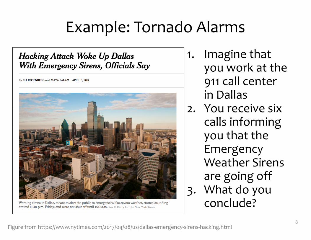
Example: Tornado Alarms1. Imagine that
you work at the 911 call center in Dallas
2. You receive six calls informing you that the Emergency Weather Sirens are going off
3. What do you conclude?
7Figure from https://www.nytimes.com/2017/04/08/us/dallas-‐emergency-‐sirens-‐hacking.html
Example: Tornado Alarms1. Imagine that
you work at the 911 call center in Dallas
2. You receive six calls informing you that the Emergency Weather Sirens are going off
3. What do you conclude?
8Figure from https://www.nytimes.com/2017/04/08/us/dallas-‐emergency-‐sirens-‐hacking.html
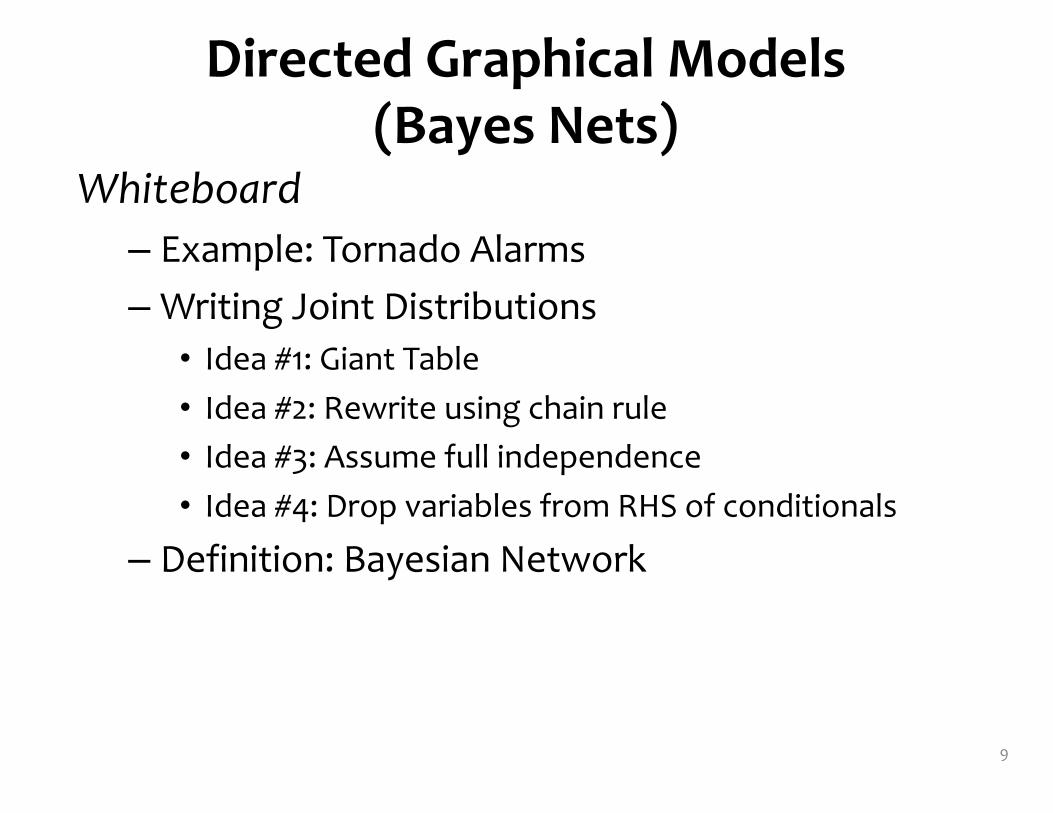
Directed Graphical Models (Bayes Nets)
Whiteboard– Example: Tornado Alarms–Writing Joint Distributions• Idea #1: Giant Table• Idea #2: Rewrite using chain rule• Idea #3: Assume full independence• Idea #4: Drop variables from RHS of conditionals
– Definition: Bayesian Network
9

Bayesian Network
10
p(X1, X2, X3, X4, X5) =
p(X5|X3)p(X4|X2, X3)
p(X3)p(X2|X1)p(X1)
X1
X3X2
X4 X5
Bayesian Network
• A Bayesian Network is a directed graphical model• It consists of a graph G and the conditional probabilities P• These two parts full specify the distribution:
– Qualitative Specification: G– Quantitative Specification: P
11
X1
X3X2
X4 X5
Definition:
P(X1…Xn ) = P(Xi | parents(Xi ))i=1
n
∏
Qualitative Specification
• Where does the qualitative specification come from?
– Prior knowledge of causal relationships– Prior knowledge of modular relationships– Assessment from experts– Learning from data (i.e. structure learning)–We simply link a certain architecture (e.g. a layered graph)
–…
© Eric Xing @ CMU, 2006-‐2011 12
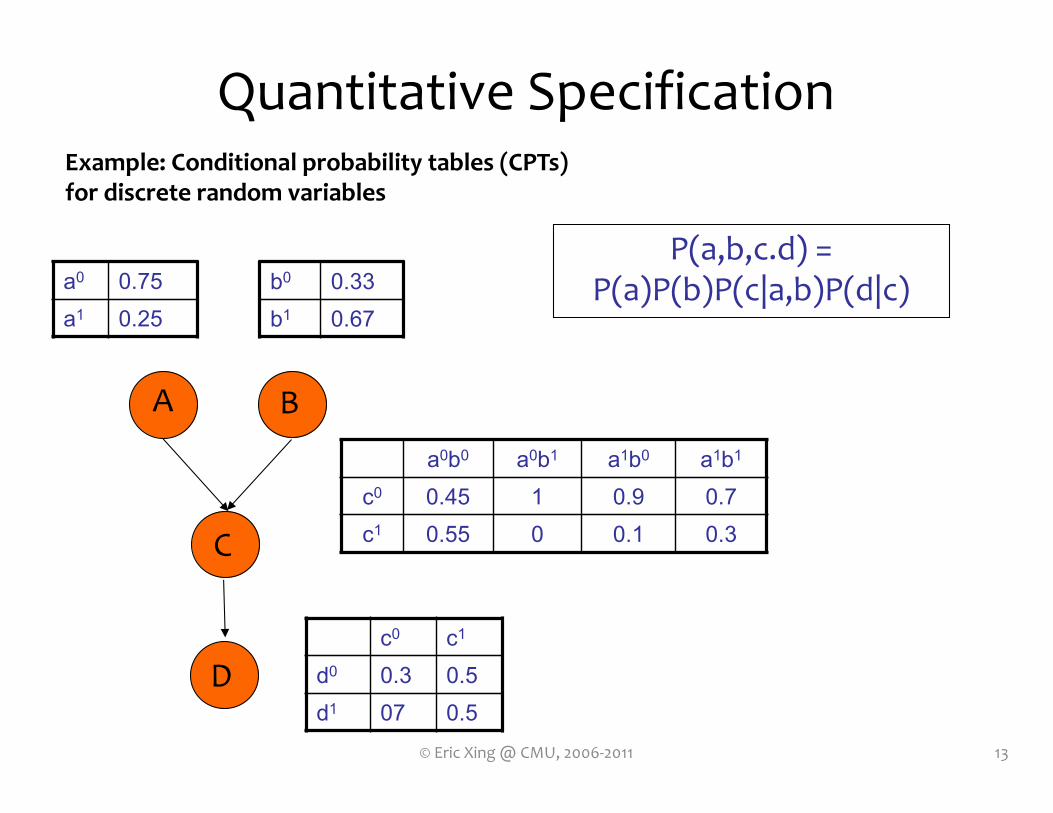
a0 0.75a1 0.25
b0 0.33b1 0.67
a0b0 a0b1 a1b0 a1b1
c0 0.45 1 0.9 0.7c1 0.55 0 0.1 0.3
A B
C
P(a,b,c.d) = P(a)P(b)P(c|a,b)P(d|c)
Dc0 c1
d0 0.3 0.5d1 07 0.5
Quantitative Specification
13© Eric Xing @ CMU, 2006-‐2011
Example: Conditional probability tables (CPTs)for discrete random variables
A B
C
P(a,b,c.d) = P(a)P(b)P(c|a,b)P(d|c)
D
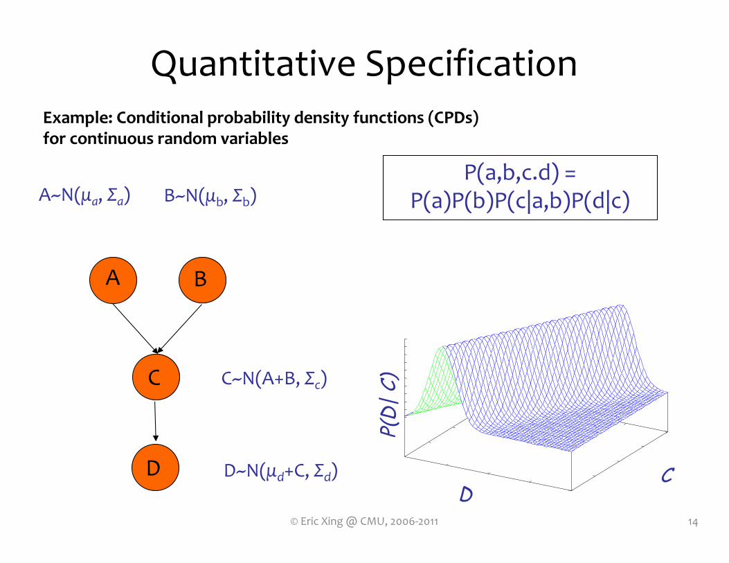
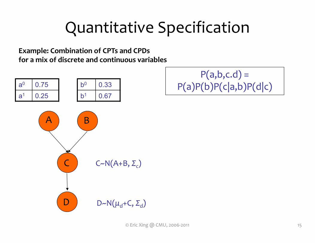
A~N(μa, Σa) B~N(μb, Σb)
C~N(A+B, Σc)
D~N(μd+C, Σd)D
C
P(D|
C)
Quantitative Specification
14© Eric Xing @ CMU, 2006-‐2011
Example: Conditional probability density functions (CPDs)for continuous random variables
A B
C
P(a,b,c.d) = P(a)P(b)P(c|a,b)P(d|c)
D
C~N(A+B, Σc)
D~N(μd+C, Σd)
Quantitative Specification
15© Eric Xing @ CMU, 2006-‐2011
Example: Combination of CPTs and CPDs for a mix of discrete and continuous variables
a0 0.75a1 0.25
b0 0.33b1 0.67
Directed Graphical Models (Bayes Nets)
Whiteboard– Observed Variables in Graphical Model– Familiar Models as Bayes Nets• Bernoulli Naïve Bayes• Gaussian Naïve Bayes• Gaussian Mixture Model (GMM)• Gaussian Discriminant Analysis• Logistic Regression• Linear Regression• 1D Gaussian
16
GRAPHICAL MODELS:DETERMINING CONDITIONAL INDEPENDENCIES
Slide from William Cohen
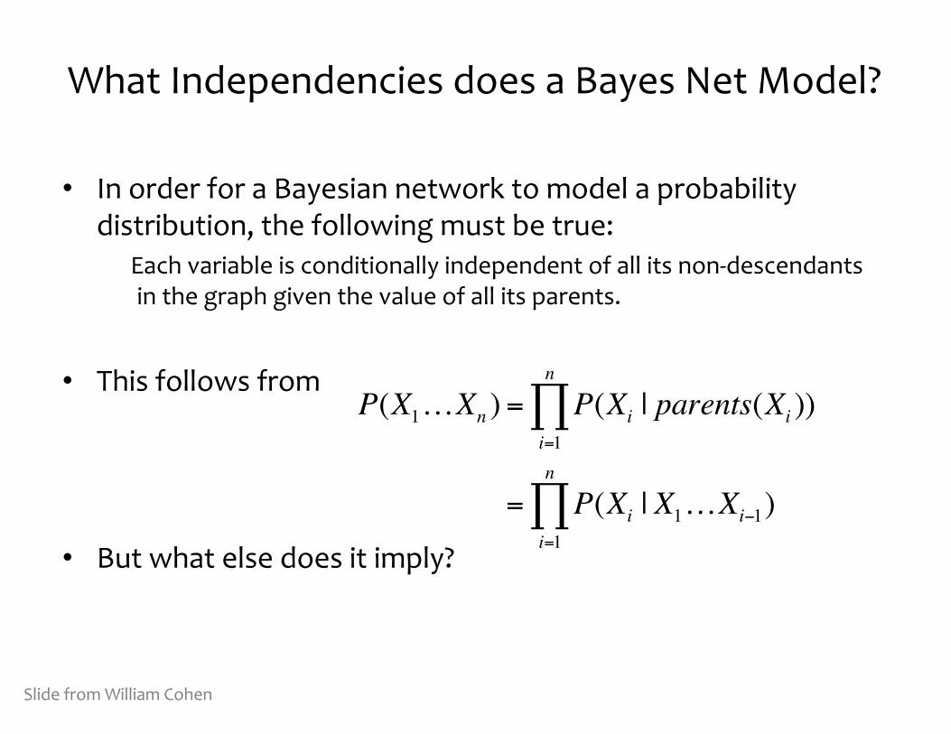
What Independencies does a Bayes Net Model?
• In order for a Bayesian network to model a probability distribution, the following must be true:
Each variable is conditionally independent of all its non-‐descendants in the graph given the value of all its parents.
• This follows from
• But what else does it imply?
P(X1…Xn ) = P(Xi | parents(Xi ))i=1
n
∏
= P(Xi | X1…Xi−1)i=1
n
∏
Slide from William Cohen
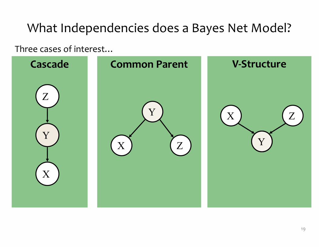
Common Parent V-‐StructureCascade
What Independencies does a Bayes Net Model?
19
Three cases of interest…
Z
Y
X
Y
X Z
ZX
YY

Common Parent V-‐StructureCascade
What Independencies does a Bayes Net Model?
20
Z
Y
X
Y
X Z
ZX
YY
X �� Z | Y X �� Z | Y X ��� Z | Y
Knowing Y decouples X and Z
Knowing Y couples X and Z
Three cases of interest…
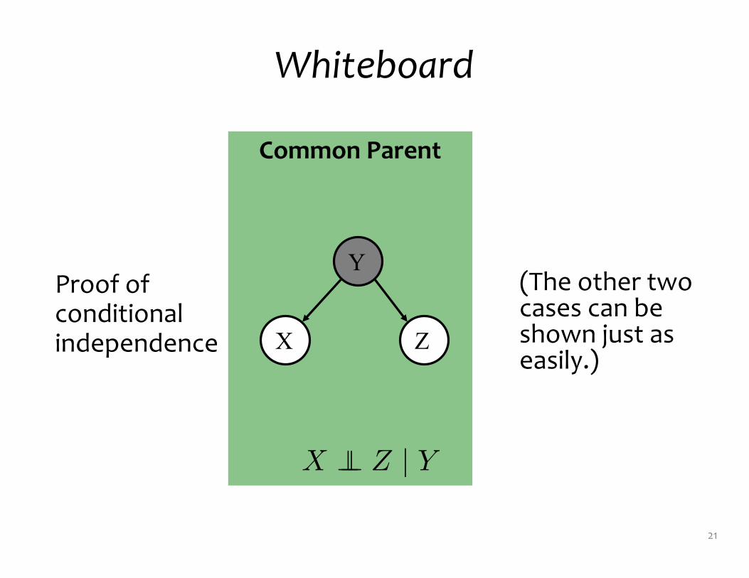
Whiteboard
(The other two cases can be shown just as easily.)
21
Common Parent
Y
X Z
X �� Z | Y
Proof of conditional independence
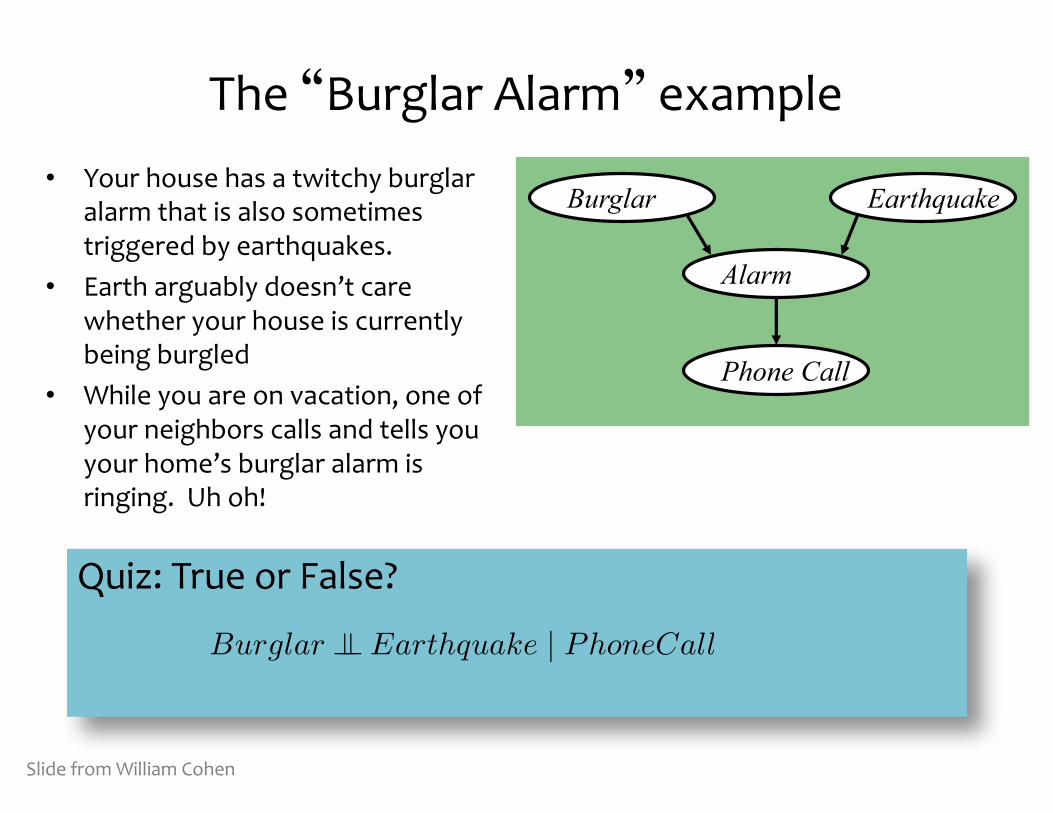
The “Burglar Alarm” example• Your house has a twitchy burglar
alarm that is also sometimes triggered by earthquakes.
• Earth arguably doesn’t care whether your house is currently being burgled
• While you are on vacation, one of your neighbors calls and tells you your home’s burglar alarm is ringing. Uh oh!
Burglar Earthquake
Alarm
Phone Call
Slide from William Cohen
Quiz: True or False?
Burglar �� Earthquake | PhoneCall
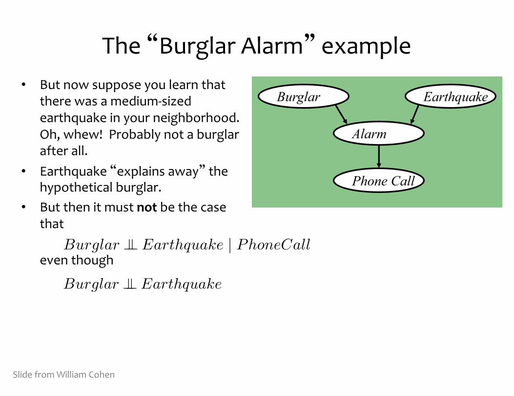
The “Burglar Alarm” example• But now suppose you learn that
there was a medium-‐sized earthquake in your neighborhood. Oh, whew! Probably not a burglar after all.
• Earthquake “explains away” the hypothetical burglar.
• But then it must not be the case that
even though
Burglar Earthquake
Alarm
Phone Call
Slide from William Cohen
Burglar �� Earthquake | PhoneCall
Burglar �� Earthquake
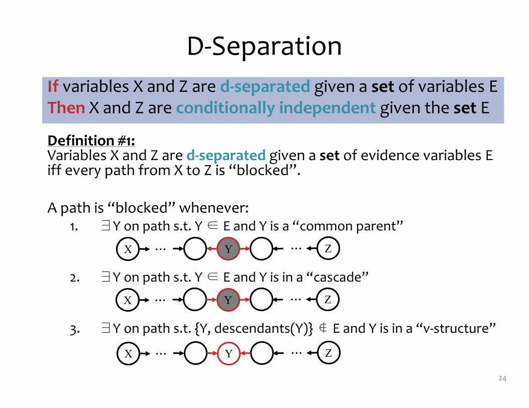
D-‐Separation
Definition #1: Variables X and Z are d-‐separated given a set of evidence variables E iff every path from X to Z is “blocked”.
A path is “blocked” whenever:1. ∃Y on path s.t. Y ∈ E and Y is a “common parent”
2. ∃Y on path s.t. Y ∈ E and Y is in a “cascade”
3. ∃Y on path s.t. {Y, descendants(Y)} ∉ E and Y is in a “v-‐structure”
24
If variables X and Z are d-‐separated given a set of variables EThen X and Z are conditionally independent given the set E
YX Z… …
YX Z… …
YX Z… …
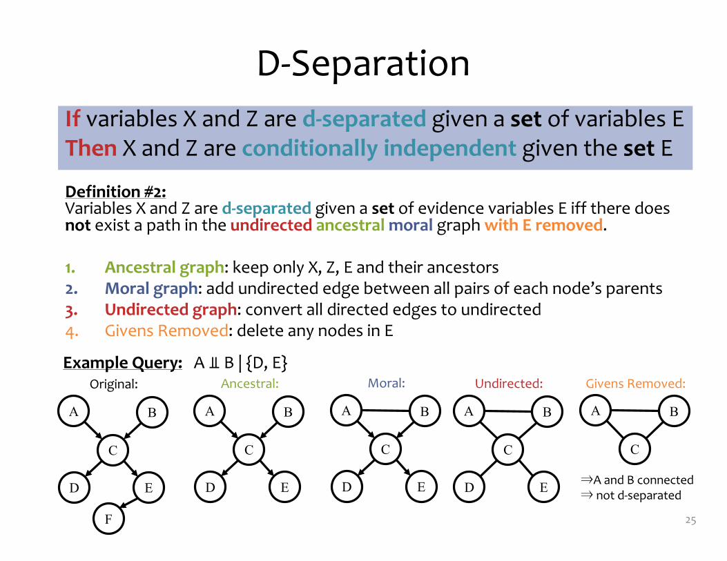
D-‐Separation
Definition #2: Variables X and Z are d-‐separated given a set of evidence variables E iff there does not exist a path in the undirected ancestral moral graph with E removed.
1. Ancestral graph: keep only X, Z, E and their ancestors2. Moral graph: add undirected edge between all pairs of each node’s parents3. Undirected graph: convert all directed edges to undirected4. Givens Removed: delete any nodes in E
25
If variables X and Z are d-‐separated given a set of variables EThen X and Z are conditionally independent given the set E
⇒A and B connected⇒ not d-‐separated
A B
C
D E
F
Original:
A B
C
D E
Ancestral:
A B
C
D E
Moral:
A B
C
D E
Undirected:
A B
C
Givens Removed:Example Query: A ⫫ B | {D, E}
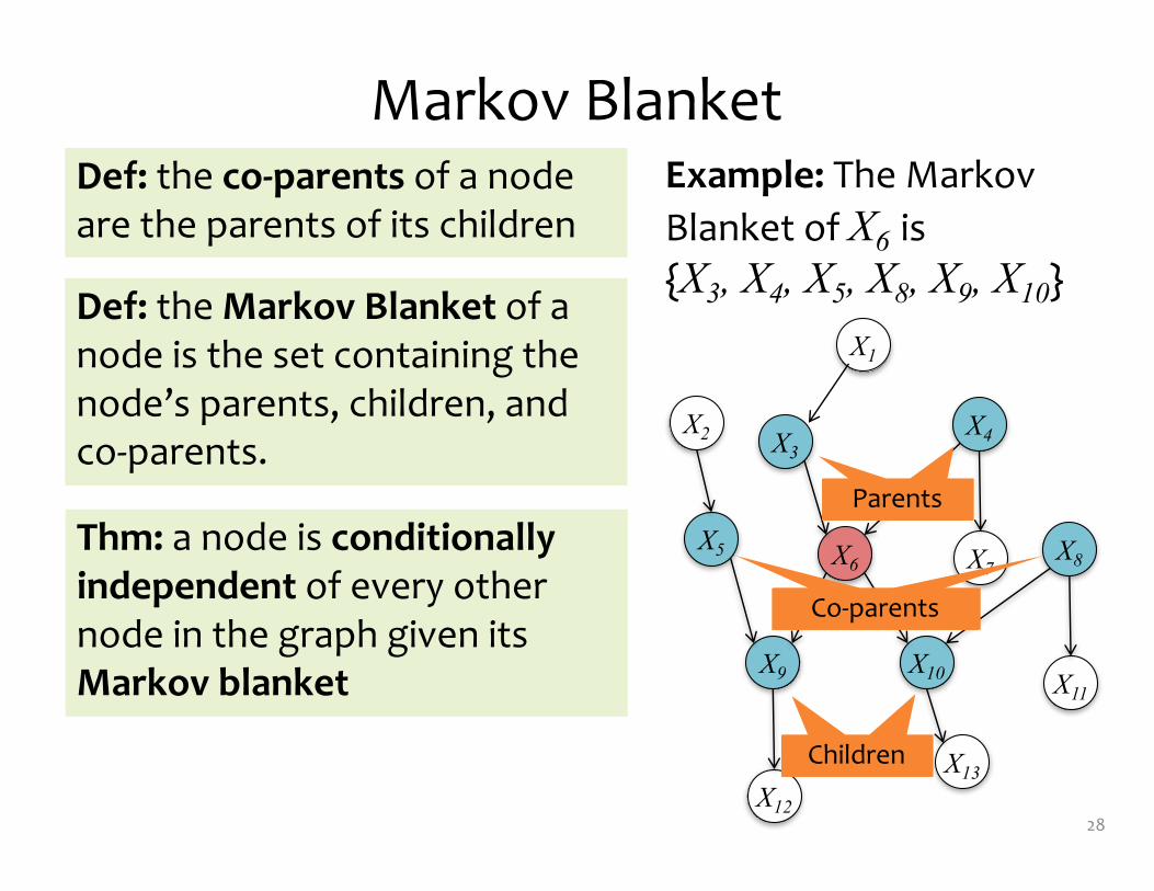
Markov Blanket
26
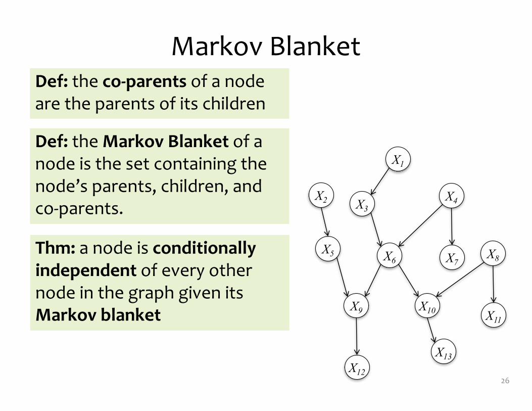
Def: the Markov Blanket of a node is the set containing the node’s parents, children, and co-‐parents.
Def: the co-‐parents of a node are the parents of its children
Thm: a node is conditionally independent of every other node in the graph given its Markov blanket
X1
X4X3
X6 X7
X9
X12
X5
X2
X8
X10
X13
X11

Markov Blanket
27
Def: the Markov Blanket of a node is the set containing the node’s parents, children, and co-‐parents.
Def: the co-‐parents of a node are the parents of its children
Thm: a node is conditionally independent of every other node in the graph given its Markov blanket
X1
X4X3
X6 X7
X9
X12
X5
X2
X8
X10
X13
X11
Example: The Markov Blanket of X6 is {X3, X4, X5, X8, X9, X10}
Markov Blanket
28
Def: the Markov Blanket of a node is the set containing the node’s parents, children, and co-‐parents.
Def: the co-‐parents of a node are the parents of its children
Thm: a node is conditionally independent of every other node in the graph given its Markov blanket
X1
X4X3
X6 X7
X9
X12
X5
X2
X8
X10
X13
X11
Example: The Markov Blanket of X6 is {X3, X4, X5, X8, X9, X10}
ParentsChildren
ParentsCo-‐parents
ParentsParents
SUPERVISED LEARNING FOR BAYES NETS
29
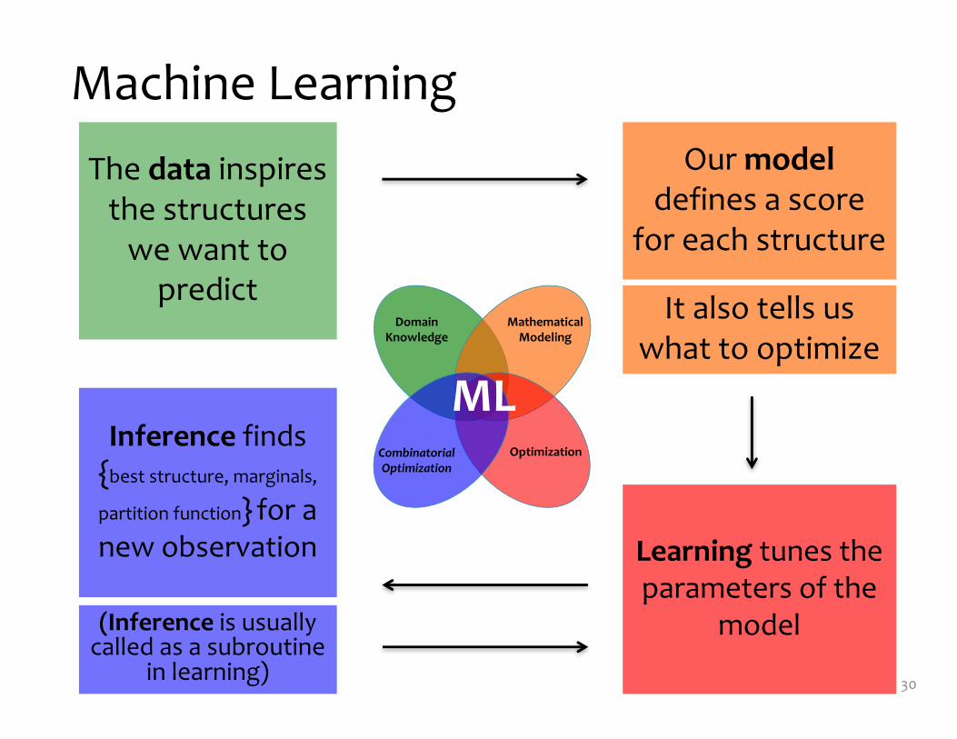
Machine Learning
30
The data inspires the structures we want to predict It also tells us
what to optimize
Our modeldefines a score
for each structure
Learning tunes the parameters of the
model
Inference finds {best structure, marginals,
partition function} for a new observation
Domain Knowledge
Mathematical Modeling
OptimizationCombinatorial Optimization
ML
(Inference is usually called as a subroutine
in learning)
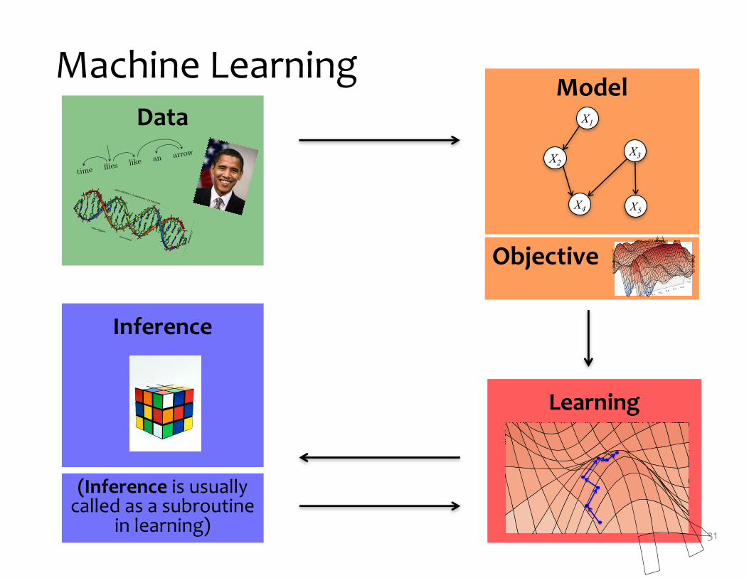
Machine Learning
31
DataModel
Learning
Inference
(Inference is usually called as a subroutine
in learning)
3
A
l
i
c
e
s
a
w
B
o
b
o
n
a
h
i
l
l
w
i
t
h
a
t
e
l
e
s
c
o
p
e
A
l
i
c
e
s
a
w
B
o
b
o
n
a
h
i
l
l
w
i
t
h
a
t
e
l
e
s
c
o
p
e
4
t
i
m
e
fl
i
e
s
l
i
k
e
a
n
a
r
r
o
w
t
i
m
e
fl
i
e
s
l
i
k
e
a
n
a
r
r
o
w
t
i
m
e
fl
i
e
s
l
i
k
e
a
n
a
r
r
o
w
t
i
m
e
fl
i
e
s
l
i
k
e
a
n
a
r
r
o
w
t
i
m
e
fl
i
e
s
l
i
k
e
a
n
a
r
r
o
w
2
Objective
X1
X3X2
X4 X5
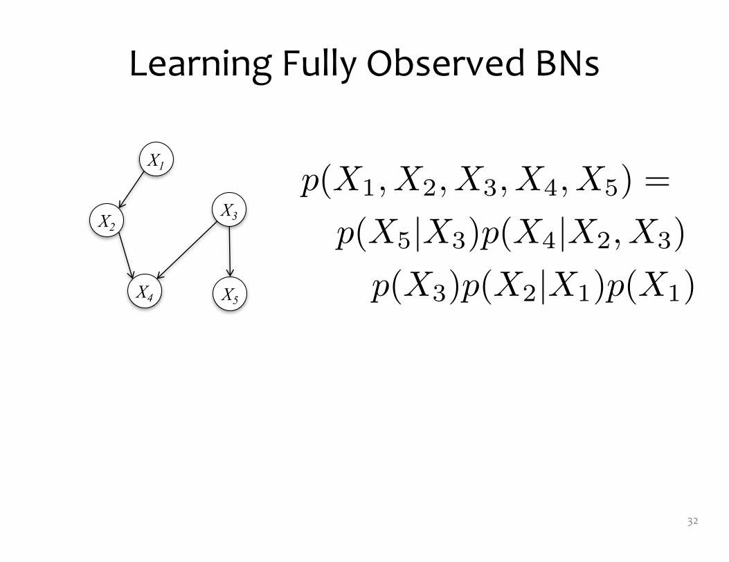
Learning Fully Observed BNs
32
X1
X3X2
X4 X5
p(X1, X2, X3, X4, X5) =
p(X5|X3)p(X4|X2, X3)
p(X3)p(X2|X1)p(X1)

p(X1, X2, X3, X4, X5) =
p(X5|X3)p(X4|X2, X3)
p(X3)p(X2|X1)p(X1)
Learning Fully Observed BNs
33
X1
X3X2
X4 X5

p(X1, X2, X3, X4, X5) =
p(X5|X3)p(X4|X2, X3)
p(X3)p(X2|X1)p(X1)
Learning Fully Observed BNs
How do we learn these conditional and marginal distributions for a Bayes Net?
34
X1
X3X2
X4 X5
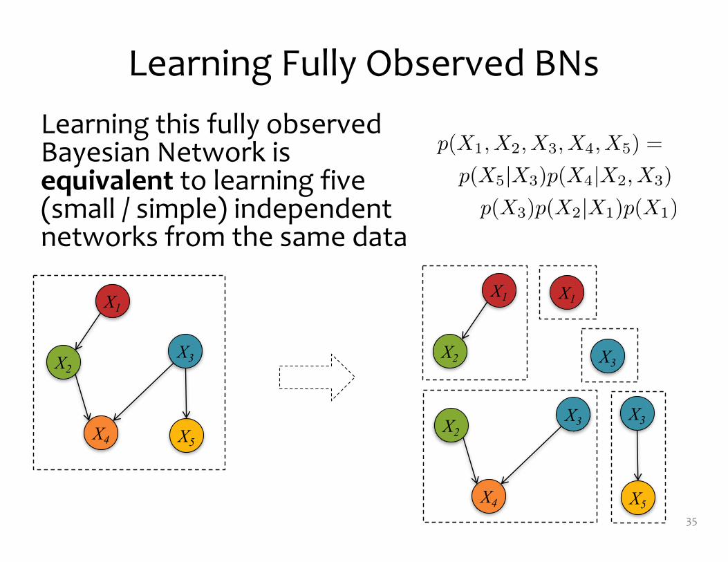
Learning Fully Observed BNs
35
X1
X3X2
X4 X5
p(X1, X2, X3, X4, X5) =
p(X5|X3)p(X4|X2, X3)
p(X3)p(X2|X1)p(X1)
X1
X2
X1
X3
X3X2
X4
X3
X5
Learning this fully observed Bayesian Network is equivalent to learning five (small / simple) independent networks from the same data

Learning Fully Observed BNs
36
X1
X3X2
X4 X5
✓⇤= argmax
✓log p(X1, X2, X3, X4, X5)
= argmax
✓log p(X5|X3, ✓5) + log p(X4|X2, X3, ✓4)
+ log p(X3|✓3) + log p(X2|X1, ✓2)
+ log p(X1|✓1)
✓⇤1 = argmax
✓1
log p(X1|✓1)
✓⇤2 = argmax
✓2
log p(X2|X1, ✓2)
✓⇤3 = argmax
✓3
log p(X3|✓3)
✓⇤4 = argmax
✓4
log p(X4|X2, X3, ✓4)
✓⇤5 = argmax
✓5
log p(X5|X3, ✓5)
✓⇤= argmax
✓log p(X1, X2, X3, X4, X5)
= argmax
✓log p(X5|X3, ✓5) + log p(X4|X2, X3, ✓4)
+ log p(X3|✓3) + log p(X2|X1, ✓2)
+ log p(X1|✓1)
How do we learn these conditional and marginal
distributions for a Bayes Net?
Learning Fully Observed BNs
Whiteboard– Example: Learning for Tornado Alarms
37