b:/documents/classes/mth 176/notes latex/chapter07 stewart6e · cscudu = −ln|cscu+cotu|+c 12....

Chapter 7 Notes, Stewart 6e Chalmeta

7.1 Integration by Parts

Introduction

If the techniques/formulas we introduced earlier do not work then there is another technique that you

can use: Integration by Parts. It is a way of simplifying integrals of the form

∫

f(x)g(x)dx in which f(x)

can be differentiated repeatedly and g(x) can be integrated repeatedly without difficulty.

The Formula

A. Derivation of the Formula The formula for integration by parts comes from the Product Rule.

d

dx(uv) = u

dv

dx+ v

du

dxd(uv) = udv + v du (differential form)

udv = d(uv) − v du (Solve for udv )∫

udv = uv −∫

v du (integrating both sides)

B. Note: The integration by parts expresses one integral,∫

v du in terms of another,∫

udv. The idea isthat with a proper choice of u and v, the second integral is easier to integrate than the original. Youmay have to use this technique several times before you reach an integral that you can integrate easily.

C. The Integration-by-Parts Formula

1. Indefinite Integrals

If u(x) and v(x) are functions of x and have continuous derivatives, then

∫

udv = uv −∫

v du

2. Definite Integrals∫ b

audv = uv

∣

∣

∣

∣

b

a

−∫ b

av du

D. How to pick u and dv

When deciding on your choice for u and dv, use the acronym: ILATE with the higher one having thepriority for u.

I -inverse trig functions

L -logarithmic functions

A -algebraic functions

T -trigonometric functions

E -exponential functions

1


Example 7.1.1.

∫

3xe2x dx

Example 7.1.2.

∫

lnxdx

Example 7.1.3.

∫ e

1x2 lnxdx

2


Example 7.1.4.

∫

√3

1tan−1 xdx

Example 7.1.5.

∫

y2e3y dy

3


Example 7.1.6.

∫

t4 sin (2t)dt

Example 7.1.7.

∫

ex cos (4x)dx

Example 7.1.8. Use the reduction formula

∫

secn udu =1

n − 1tan u secn−2 u +

n − 2

n − 1

∫

secn−2 udu

∫

sec4 y dy

4


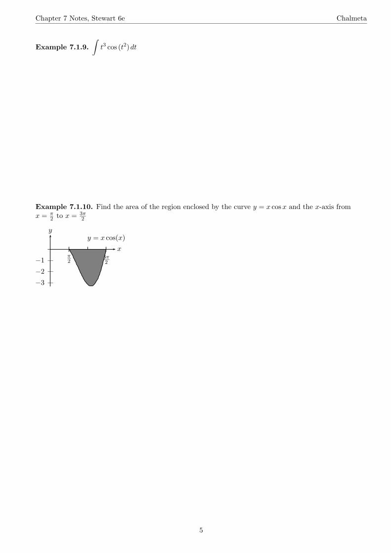
Example 7.1.9.

∫

t3 cos (t2)dt

Example 7.1.10. Find the area of the region enclosed by the curve y = x cos x and the x-axis fromx = π

2 to x = 3π2

x

y

ππ2

3π2

y = x cos(x)

−1

−2

−3

5


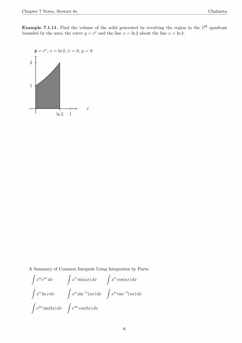
Example 7.1.11. Find the volume of the solid generated by revolving the region in the 1st quadrantbounded by the axes, the curve y = ex and the line x = ln 2 about the line x = ln 2.

x

y

ln 2

y = ex, x = ln 2, x = 0, y = 0

1

2

1

A Summary of Common Integrals Using Integration by Parts:∫

xneax dx

∫

xn sin(ax)dx

∫

xn cos(ax)dx

∫

xn lnxdx

∫

xn sin−1(ax)dx

∫

xn tan−1(ax)dx

∫

eax sin(bx)dx

∫

eax cos(bx)dx

6


7.2 Trigonometric Integrals

7.2.1 Evaluating

∫

sinm x cosn(x)dx

A. If the power of cosine is odd (n = 2k + 1), save one cosine factor and use cos2 x = 1− sin2 x to expressthe remaining factors in terms of sine:

∫

sinm x cos2k+1 xdx =

∫

sinm x cos2k x cos xdx

=

∫

sinm x(

cos2 x)k

cos xdx

=

∫

sinm x(

1 − sin2 x)k

cos xdx

Then substitute u = sinx.

B. If the power of sine is odd (m = 2k + 1), save one sine factor and use sin2 x = 1− cos2 x to express theremaining factors in terms of cosine:

∫

sin2k+1 x cosn xdx =

∫

sin2k x cosn x sinxdx

=

∫

(

sin2 x)k

cosn x sinxdx

=

∫

(

1 − cos2 x)k

cosn x sinxdx

Then substitute u = cos x.

C. If the powers of both sine and cosine are odd, either 1 or 2 can be used.

D. If the powers of both sine and cosine are even, use the half-angle identities

sin2 x =1

2[1 − cos (2x)] and cos2 x =

1

2[1 + cos (2x)]

E. It is sometimes helpful to use the identity sinx cos x = 12 sin(2x).

Example 7.2.1.

∫

sin θ cos4(θ)dθ

7


Example 7.2.2.

∫

sin3 φdφ

Example 7.2.3.

∫

sin3 √x cos3√

x√x

dx

8


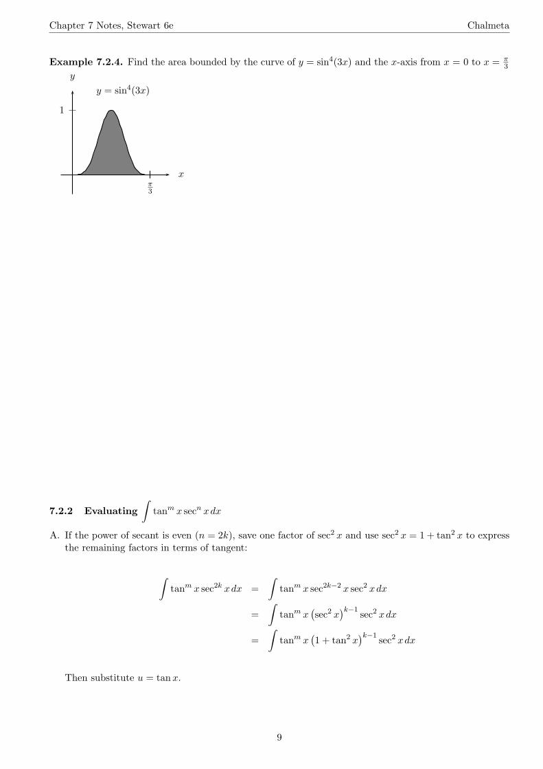
Example 7.2.4. Find the area bounded by the curve of y = sin4(3x) and the x-axis from x = 0 to x = π3

x

y

π3

y = sin4(3x)

1

7.2.2 Evaluating

∫

tanm x secn xdx

A. If the power of secant is even (n = 2k), save one factor of sec2 x and use sec2 x = 1 + tan2 x to expressthe remaining factors in terms of tangent:

∫

tanm x sec2k xdx =

∫

tanm x sec2k−2 x sec2 xdx

=

∫

tanm x(

sec2 x)k−1

sec2 xdx

=

∫

tanm x(

1 + tan2 x)k−1

sec2 xdx

Then substitute u = tanx.

9


B. If the power of tangent is odd (m = 2k + 1), save one factor of sec x tanx and use tan2 x = sec2 x − 1to express the remaining factors in terms of secant:

∫

tan2k+1 x secn xdx =

∫

tan2k x secn−1 x sec x tanxdx

=

∫

(

tan2 x)k

secn−1 x sec x tanxdx

=

∫

(

sec2 x − 1)k

secn−1 x sec x tan xdx

Then substitute u = sec x.

Example 7.2.5.

∫

tan6 y dy

Example 7.2.6.

∫ π/6

0tan θ sec3 θ dθ

10


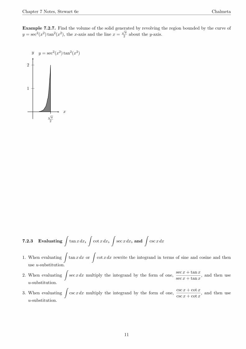
Example 7.2.7. Find the volume of the solid generated by revolving the region bounded by the curve of

y = sec2(x2) tan2(x2), the x-axis and the line x =√

π2 about the y-axis.

x

y

√π

2

y = sec2(x2) tan2(x2)

1

2

7.2.3 Evaluating

∫

tanxdx,

∫

cot xdx,

∫

sec xdx, and

∫

csc xdx

1. When evaluating

∫

tan xdx or

∫

cot xdx rewrite the integrand in terms of sine and cosine and then

use u-substitution.

2. When evaluating

∫

sec xdx multiply the integrand by the form of one,sec x + tanx

sec x + tanx, and then use

u-substitution.

3. When evaluating

∫

csc xdx multiply the integrand by the form of one,csc x + cotx

csc x + cotx, and then use

u-substitution.

11


7.3 Trigonometric Substitution

Introduction

Consider the integral∫

x√

a2 − x2 dx. The substitution of u = a2 − x2 will allow us to integrate thisintegral.

Now consider∫ √

a2 − x2 dx. We have integrated this type of integral using the area of either a half orquarter of a circle depending on the limits of integration. What if we wanted to evaluate this indefiniteintegral or the definite integral in which the limits do not define either a half or quarter of a circle? Wewill evaluate this type of integral using a type of substitution called inverse substitution.

7.3.1 Trigonometric Substitution for Integrals Involving√

a2 − x2,√

a2 + x2,√

x2 − a2

Radical Substitution Restrictions on θ Identiy

√a2 − x2 x = a sin θ −π

2 ≤ θ ≤ π2 1 − sin2 θ = cos2 θ

√a2 + x2 x = a tan θ −π

2 ≤ θ ≤ π2 1 + tan2 θ = sec2 θ

√x2 − a2 x = a sec θ 0 ≤ θ ≤ π, θ 6= π

2 sec2 θ − 1 = tan2 θ

Example 7.3.1. Evaluate∫ √

a2 − x2 dx

13


Simplifications of the trigonometric substitutions

1.√

a2 − x2 =√

a2 − a2 sin2 θ =√

a2 cos2 θ = |a cos θ| = a cos θ

2.√

a2 + x2 =√

a2 + a2 tan2 θ =√

a2 sec2 θ = |a sec θ| = a sec θ

3.√

x2 − a2 =√

a2 sec2 θ − a2 =√

a2 tan2 θ = |a tan θ| = a tan θ

Example 7.3.2. Evaluate

∫

dx√9 + x2


∫ 4

2

√x2 − 4

xdx

14



∫

√4 − x2

x2dx


∫

dx

(5 − 4x − x2)5/2

15


7.4 Integration of Rational Functions by Partial Fractions

7.4.1 Reducing an Improper Fraction (long division)

When the degree of the numerator is greater than or equal to the degree of the denominator, we will beusing long division to simplify the integrand. Sometimes after doing long division, you will have a remainderthat will be placed on top of the divisor; this part of the new integrand may result after integration ineither a natural logarithm or an arctangent.

∫

dx

x2 + a2=

1

atan−1

(x

a

)

+ c


∫

x2 + 7x − 3

x + 4dx


∫

5x5 + 28x

x4 + 9dx

16



∫ 3

−1

4x2 − 7

2x + 3dx

7.4.2 Partial Fractions

Partial Fractions consists of decomposing a rational function into simpler component fractions and thenevaluating the integral term by term.

Example 7.4.4. Denominator is a product of disctinct linear factors∫

3x + 7

x2 + 6x + 5dx

17


Example 7.4.5. Denominator is a product of linear factors, some of which are repeated.∫

3x2 − 8x + 13

(x + 3)(x − 1)2dx

Example 7.4.6. Denominator contains irreducible quadratic factors, none of which is repeated.∫

2x2 + x − 8

x3 + 4xdx

18


7.4.3 Rationalizing substitutions

Some nonrational functions can be changed into rational functions by means of appropriate substitutions.

Example 7.4.7.

∫ √x

x − 4dx

7.4.4 Additional Examples


∫

2x + 1

x2 + 2x − 3dx

19



∫

x2 − x − 21

(x2 + 4)(2x − 1)dx


∫

4x2 + 3x + 6

x2(x2 + 3)dx

20



∫

ey

√16 − e2y

dy


∫

dx

1 + ex


∫

e2t

et − 2dt

21



∫

√

x2 + x + 1dx

22


7.5 Strategy for Integration

7.5.1 Basic Integration Formulas

1.

∫

du = u + C 2.

∫

k · f(x)dx = k

∫

f(x)dx

3.

∫

(du ± dv) dx =

∫

du ±∫

dv 4.

∫

un du =un+1

n + 1+ C; n ∈ R, n 6= −1

5.

∫

1

udu = ln |u| + C 6.

∫

eu dx = eu + C

7.

∫

au du =au

ln a+ C 8.

∫

sinudu = − cos u + C

9.

∫

cos udu = sinu + C 10.

∫

sec2 udu = tanu + C

11.

∫

csc2 udu = − cot u + C 12.

∫

sec u tan udu = sec u + C

13.

∫

csc u cot udu = − csc u + C

14.

∫

tan udu =

∫

sin u

cos udu = − ln | cos u| + C = ln | sec u| + C

15.

∫

cot udu =

∫

cos u

sin udu = ln | sinu| + C = − ln | csc u| + C

16.

∫

sec udu =

∫

sec u

(

sec u + tanu

sec u + tanu

)

du =

∫(

sec2 u + sec u tan u

sec u + tanu

)

du = ln | sec u + tanu| + C

17.

∫

csc udu =

∫

csc u

(

csc u + cot u

csc u + cot u

)

du =

∫(

csc2 u + csc u cot u

csc u + cotu

)

du = − ln | csc u + cotu| + C

18.

∫

du√a2 − u2

= sin−1 u

a+ C 19.

∫

du

a2 + u2=

1

atan−1 u

a+ C

20.

∫

du

u√

u2 − a2=

1

asec−1

∣

∣

∣

u

a

∣

∣

∣+ C

21.

∫

du

u2 − a2=

1

2aln

∣

∣

∣

∣

u − a

u + a

∣

∣

∣

∣

+ C 22.

∫

du√u2 ± a2

= ln∣

∣

∣u +

√

u2 ± a2∣

∣

∣+ C

23


7.5.2 Procedures for matching integrals to basic formulas

1. Simplify the integrand.2. Make a simplifying substitution (u-substitution).3. Compete the square.4. Use a trigonometric identity / make a trigonometric substitution.5. Eliminate a square root.6. Reduce an improper fraction.7. Separate a fraction / partial fractions.8. Multiply by a form of 1.9. Use integration by parts

Example 7.5.1.

∫

xex2

dx

Example 7.5.2.

∫

xe2x dx

Example 7.5.3.

∫

x3ex2

dx

24


Example 7.5.4.

∫

8

x2 − 6x + 9dx

Example 7.5.5.

∫

2x2 − x + 4

x3 + 4xdx

Example 7.5.6.

∫

dx

x2√

x2 + 4

25


Example 7.5.7.

∫

sin2 x cos5 xdx

Example 7.5.8.

∫

ex

sin(ex)dx

Example 7.5.9.

∫

dx√6 − x2 + 10x

dx

26


Example 7.5.10.

∫ π

4

0

√

1 + cos(4x)dx

Example 7.5.11.

∫

(√

x + 10)3√x

dx

Example 7.5.12.

∫

x5 sec5(3x6) tan3(3x6)dx

27


7.6 Integral Tables

The Basic techniques of integration are substitution and integration by parts; these techniques transformunfamiliar integrals into integrals whose forms are recognizable or can be found in a table. The integraltables were created by applying substitutions and integration by parts to generic integrals in order to savethe trouble of repeating laborious calculations. When an integral matches an integral in the table or canbe changed into one of the tabulated integrals through algebra, trigonometry substitution or calculus, thetables give a ready made solution for the problem.

Example 7.6.1.

∫

dx

x√

3x + 4Formula #

Example 7.6.2.

∫

dy√

1 + 9y2Formula #

28


Example 7.6.3.

∫

√

5 + sin(4θ) cot(4θ)dθ Formula #

Example 7.6.4.

∫ √x√

1 − xdx Formula #

29


Example 7.6.5.

∫

dx

x3√

3 − x4Formula #

Example 7.6.6.

∫

√x − x2

xdx Formula #

30


Example 7.6.7.

∫

cot4 (3x)dx Formula #

Example 7.6.8.

∫

dx

x√

7 − x2Formula #

31


7.7 Approximate Integration

NOTE: Approximate/numerical integration is used when either we cannot find an antiderivative to aproblem or one does not exist.

7.7.1 Midpoint Rule

A. Formula∫ b

af(x)dx ≈ Mn =

n∑

i=1

f(x̄i) · ∆x = ∆x [f(x̄1) + f(x̄2) + · · · + f(x̄n)]

Where ∆x =b − a

nand x̄i =

xi−1 + xi

2= midpoint of [xi−1, xi].

B. The Error Estimate for the Midpoint Rule, EM .

1. EM =

∫ b

af(x)dx − Mn, where Mn is the Midpoint Rule.

2. If f ′′ is continuous and K is any upper bound for the values of |f ′′| on [a, b], then

|EM | ≤(

b − a

24

)

(∆x)2K ≤(

(b − a)3

24n2

)

K, where ∆x =b − a

n

Example 7.7.1. Use the Midpoint Rule to estimate

∫ 1

−1(x2 + 1)dx using n = 4. Find the error in the

midpoint approximation, EM .

32


7.7.2 Trapezoidal Rule

A. Formula

One way to approximate a definite integral is by the use of n trapezoids rather than rectangles. In thedevelopment of this method we will assume that the function f(x) is continuous and positive valued on

the interval [a, b] and that

∫ b

af(x)dx represents the area of the region bounded by the graph of f(x)

and the x-axis, from x = a to x = b.

Partition the interval [a, b] into n equal subintervals, each of width ∆x =b − a

nsuch that

a = x0 < x1 < x2 < · · · < xn = b.

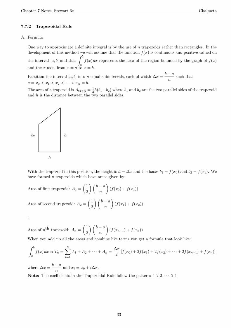
The area of a trapezoid is Atrap = 12h(b1+b2) where b1 and b2 are the two parallel sides of the trapezoid

and h is the distance between the two parallel sides.

b2 b1

h

With the trapezoid in this position, the height is h = ∆x and the bases b1 = f(x0) and b2 = f(x1). Wehave formed n trapezoids which have areas given by:

Area of first trapezoid: A1 =

(

1

2

)(

b − a

n

)

(f(x0) + f(x1))

Area of second trapezoid: A2 =

(

1

2

)(

b − a

n

)

(f(x1) + f(x2))

...

Area of nth trapezoid: An =

(

1

2

)(

b − a

n

)

(f(xn−1) + f(xn))

When you add up all the areas and combine like terms you get a formula that look like:

∫ b

af(x)dx ≈ Tn =

n∑

i=1

A1 + A2 + · · · + An =∆x

2[f(x0) + 2f(x1) + 2f(x2) + · · · + 2f(xn−1) + f(xn)]

where ∆x =b − a

nand xi = x0 + i∆x.

Note: The coefficients in the Trapezoidal Rule follow the pattern: 1 2 2 · · · 2 1

33


B. Error Estimate for the Trapezoidal Rule, ET .

1. ET =

∫ b

af(x)dx − Tn, where Tn is the Trapezoidal Rule.

2. If f ′′ is continuous and K is any upper bound for the values of |f ′′| on [a, b], then

|ET | ≤(

b − a

12

)

(∆x)2K ≤(

(b − a)3

12n2

)


n

Example 7.7.2. Use the Trapezoidal Rule to estimate

∫ 1

−1(x2 + 1)dx using n = 4. Find the error in the

trapezoidal approximation, ET . How large do we have to choose n so that the approximation Tn to the

integral

∫ 1

−1(x2 + 1)dx is accurate to 0.001?

34


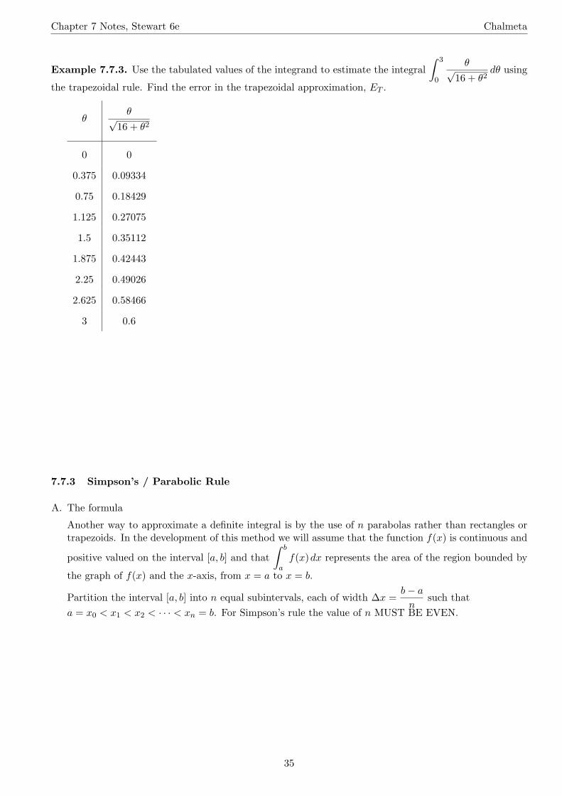
Example 7.7.3. Use the tabulated values of the integrand to estimate the integral

∫ 3

0

θ√16 + θ2

dθ using

the trapezoidal rule. Find the error in the trapezoidal approximation, ET .

θθ√

16 + θ2

0 0

0.375 0.09334

0.75 0.18429

1.125 0.27075

1.5 0.35112

1.875 0.42443

2.25 0.49026

2.625 0.58466

3 0.6

7.7.3 Simpson’s / Parabolic Rule

A. The formula

Another way to approximate a definite integral is by the use of n parabolas rather than rectangles ortrapezoids. In the development of this method we will assume that the function f(x) is continuous and

positive valued on the interval [a, b] and that

∫ b

af(x)dx represents the area of the region bounded by

the graph of f(x) and the x-axis, from x = a to x = b.

Partition the interval [a, b] into n equal subintervals, each of width ∆x =b − a

nsuch that

a = x0 < x1 < x2 < · · · < xn = b. For Simpson’s rule the value of n MUST BE EVEN.

35


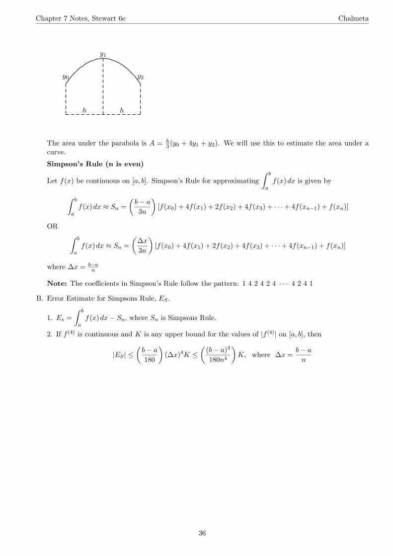
y0

y1

y2

h h

The area under the parabola is A = h3 (y0 + 4y1 + y2). We will use this to estimate the area under a

curve.

Simpson’s Rule (n is even)

Let f(x) be continuous on [a, b]. Simpson’s Rule for approximating

∫ b

af(x)dx is given by

∫ b

af(x)dx ≈ Sn =

(

b − a

3n

)

[f(x0) + 4f(x1) + 2f(x2) + 4f(x3) + · · · + 4f(xn−1) + f(xn)]

OR

∫ b

af(x)dx ≈ Sn =

(

∆x

3n

)

[f(x0) + 4f(x1) + 2f(x2) + 4f(x3) + · · · + 4f(xn−1) + f(xn)]

where ∆x = b−an

Note: The coefficients in Simpson’s Rule follow the pattern: 1 4 2 4 2 4 · · · 4 2 4 1

B. Error Estimate for Simpsons Rule, ES .

1. Es =

∫ b

af(x)dx − Sn, where Sn is Simpsons Rule.

2. If f (4) is continuous and K is any upper bound for the values of |f (4)| on [a, b], then

|ES | ≤(

b − a

180

)

(∆x)4K ≤(

(b − a)3

180n4

)


n

36


Example 7.7.4. Use Simpsons Rule to estimate

∫ 1

−1(x2 + 1)dx using n = 4. Find the error in Simpson’s

approximation, ES . How large do we have to choose n so that the approximation Tn to the integral∫ 1

−1(x2 + 1)dx is accurate to 0.0001?

Example 7.7.5. Use the tabulated values of the integrand to estimate the integral

∫ 3

0

θ√16 + θ2

dθ using

Simpson’s rule. Find the error in the trapezoidal approximation, ES .

θθ√

16 + θ2

0 0

0.375 0.09334

0.75 0.18429

1.125 0.27075

1.5 0.35112

1.875 0.42443

2.25 0.49026

2.625 0.58466

3 0.6

37

b:/documents/classes/mth 176/notes latex/chapter07 stewart6e · cscudu = −ln|cscu+cotu|+c 12....

Documents