J-RA/4/3//20157

H.

Kazerooni

Reprinted fromIEEE JOURNAL OF ROBOTICS AND AUTOMATION

Vol. 4, No.3, June 1988

324 IEEE JOURNAL OF ROBOTICS AND AUTOMATION, YOLo 4, N~. 3, JUNE 1988

H. KAZEROONI

oFn, of,

(lJb

"'d"'0

Abstract-A fast, lightweight, active end effector which can beattached to the endpoint of a commercial robot manipulator has beendesigned and buill. Impedance control [11) has been developed on thisdevice. This control method causes the end effector to behave dynami-cally as a two-dimensional Remote Center Compliance (RCC). Thecompliancy in this active end effector is electronic and so can bemodulated by an on-line computer.

The device is a planar, five-bar linkage which is driven by two direct-drive, brushless dc motors. A two-dimensional, piezoelectric force cell onthe endpoint of the device, two 12-bit encoders, and two tachometers onthe motors form the measurement system. The high structural stiffnessand light weight of the material used in the system allow for a IS-Hzbandwidth impedance control.

NOMENCLATURE

E Environment dynamics.e Input trajectory.F Contact force.G Closed-loop transfer function matrix.H The compensator.j Complex number notation ..;=T:Jo Jacobian.j; Moment of inertia of each link relative to

the endpoint of the link.K Stiffness matrix.K", K, Stiffness in the direction normal and

tangential to the part.I;, m; Length and mass of each link.Mo Inertia matrix.M The grinder mass in the passive end

effector.S Sensitivity transfer function matrix.r Input command vector.T = [T1 T 2] T Torque vector.X = [X, X,,]T Vector of the tool position in the Carte-

sian coordinate frame.Xo Environment position measured in the

Cartesian coordinate frame.X;, 8; Location of the center of mass and

orientation of each link.a Small perturbation of 8. in the neighbor-

hood of 81 = 900.oe Endpoint deflection in X" direction.oX"' oX, Endpoint deflection in the direction nor-

mal and tangential to the part.

Manuscript received January 12, 1987; revised October, 6, 1987.The author is with the Mechanical Engineering Department, University of

Minnesota, Minneapolis, MN 55455.IEEE Log Number 8820157.

Contact force in the direction normal andtangential to the part.Frequency range of the burr observedfrom the robot endpoint.Dynamic manipulability.Frequency range of the operation (band-width).Frequency range of the robot oscillations."'r

0882-4967/88/0600-0324$01.00 @ 1988 IEEE

I. INTRODUCTION

M ANUFACTURING manipulations require mechanical

interaction with the environment or with the object

being manipulated. Robot manipulators are subject to interac-tion forces when they maneuver in a constrained workspace.Inserting a computer board in a slot or deburring an edge areexamples of constrained maneuvers. In constrained maneu-vers, one is concerned with not only the position of the robotendpoint, but also the contact forces. In constrained maneu-vering, the interaction forces must be accommodated ratherthan resisted. If we define compliancy as a measure of theability of the manipulators to react to interaction forces andtorques, the objective is to assure compliant motion (passivelyor actively) for the robot endpoint in the Cartesian coordinateframe for manipulators that must maneuver in the constrainedenvironments.

An example of a manufacturing manipulation that requirescompliancy is robotic assembly. To perform the assembly ofparts that are not perfectly aligned, one must use a compliantelement between the part and the robot to ease the insertionprocess. The RCC can be attached to the endpoint of the robotmanipulators [3], [20]. This device develops a passivecompliant interface between the robot and the part. Theprimary function of the RCC is to act as a filter that decreasesthe contact force between the part and the robot arising fromthe robot oscillations, robot programming error, and partfixturing errors. These end effectors are called passivebecause the elements that generate compliancy are passive andno external energy is flowing into the system.

Active end effectors are devices that can be mounted at theendpoint of the robot manipulators to develop more degrees offreedom [5]. This paper describes the design, construction,and control of an active end effector that can be used as acompliant tool holder. There is no passive compliant elementin the system, because the compliancy in the system isgenerated electronically [6], [7], [11]. The advantage of thissystem over passive systems is that one can modulate thecompliancy in the system arbitrarily by an on-line computer,

~OONI; DIRECT-DRIVE END EFFEcrOR 325

depending on the requirements of the tasks. Two dc actuators!>Ower the two degrees of freedom of the system.

Fig. 1.

link 2

Force"" SensorClampingBolt

Grinder

II. ARCHITECTURE

Fig. 1 shows the schematic diagram of the active end

effector. The end effector is a 5-bar linkage with two degrees

of freedom. All are articulated drive joints. The links are made

of aluminum 6061. The actuators are dc brushless direct-drive

motors equipped with 12-bit encoders and tachometers. The

choice of the direct-drive system eliminates backlash and

develops more structural rigidity in the system. This structural

rigidity allows for a wide control bandwidth and higher

precision. The stall torque and the peak torque for each motoris 5 lb. in and 20 lb. in, respectively. Each motor weighs 2.4

lb. A wide-bandwidth piezoelectric-based force sensor is

located between the endpoint of the mechanism and the end-

effector gripper to measure the force on the tool. The force

sensor is preloaded by a clamping bolt, and measures the forcein two dimensions in the plane of the mechanism. The entire

weight of the links with bearings and force sensor is 111.4 g.

The end effector can be attached to the robot manipulator by a

simple fixture between the housing of the motors and the robot

endpoint as shown in Fig. 2. Fig. 3 shows the side view of the

end effector.

The characteristics of this end effector are as follows:

size of the 5-bar linkage at nominal 2.167 in X

position 4.160 inheight of the end effector with motors

(excluding the grinder tool) 3.760 inlinear workspace of the endpoint 0.3 in x 0.3 in

resolution of the endpoint motion 2.6 X 10-3 inbandwidth of the control system 15 Hz

total mass of the mechanism (without the

tool) 0.25 lbweight of two motors 4.8 lb

weight of the tool 0.3 lbtotal mass (mass of the mechanism and the

motors, excluding the grinding tool) 5.05 lb.

Fig. 4 shows the size of the end effector relative to a hand.Fig. 3.

TThe side view of the force sensor assembly.

ill. MOTIVATION FOR DEVELOPMENT OF THE Acnve END

EFFECTOR

This section explains briefly a practical problem thatrequires modulation of the compliance in the system by an on-line computer. This example also shows the limitation ofpassive RCC in developing a desired stiffness for arbitraryfrequency ranges. The details of the problem are given in [8],

[10].Consider the deburring of a surface by a robot manipulator;

the objective is to use an end effector to smooth the surfacedown to the coinmanded trajectory depicted by the dashed linein Fig. 5. It is intuitive to design a system" with a largeimpedance (small compliance) in the normal direction and asmall impedance (large compliance) in the tangential direc-tion. We define impedance as the ratio of the contact force tothe end-effector deflection as a function of frequency.

A large impedance in the normal direction causes the The active end effector.Fig. 4.

"~...,c

326 IEEE JOURNAL OF ROBOTICS AND AUTOMATION, YOLo 4, NO. 3,JUNE 1988

normalforce

I'0 0; '. '. .."1 ",-

16XtlJwl/6FtlJwJl.10

tangentialforce

10

In/Lbf .0

Fig. 5. Deburring an edge. .0 ;~ -i ~, ,I I 18><nIJc.>J/8FnlJc.>J

1 I II ...1 .'0 '0' '0" '0"Rad/secFig.

6. The required dynamic behavior for deburring.

.0

Robot

£;t1

PneumaticGrinder

-I

Passive RCC

Rotary File-.

.0',

" """' " ". "" I

16XtlJwJ/6FtlJwJI-

....

endpoint of the grinder to reject the interaction forces and stayvery close to the commanded trajectory (dashed line). Thelarger the impedance of the end effector in the normaldirection, the smoother the surface will be. Given the volumeof the metal to be removed, the desired tolerance in the normaldirection prescribes an approximate value for impedance in thenormal direction. The force necessary to cut in the tangentialdirection at a constant traverse speed is approximatelyproportional to the volume of the metal to be removed [8)-[10). Therefore, the larger the burrs on the surface, the slowerthe manipulator must move in the tangential direction tomaintain a relatively constant tangential force. This is neces-sary because the slower speed of the endpoint along thesurface implies a smaller volume of metal to be removed perunit of time, and consequently, less force in the tangentialdirection. To remove the metal from the surface, the grindershould slow down in response to contact forces with largeburrs.

The above explanation demonstrates that it is necessary forthe end effector to accommodate the interaction forces alongthe tangential direction, which directly implies a smallimpedance value in the tangential direction. If a designer doesnot accommodate the interaction forces by specifying a smallstiffness value in the tangential direction, the large burrs on thesurface will produce large contact forces in that direction andconsequently stall the tool. Large contact forces in the.al d.. d 1 d fl .. h d .in/lbf ...tangentI lrectIon may eve op a e ectIon In teen pointposition in the normal direction which might exceed thedesired tolerance. A small value for the impedance in thetangential direction (relative to the impedance in the normaldirection) guarantees, small contact force in the tangentialdirection. The frequency spectrum of the roughness of thesurface and the desired translational speed of the robot alongthe surface determine the frequency range of operation, "'b.

On the other hand, for compensation of the robot oscilla- very small for the entire frequency range of the burr "'b' Whiletion, the impedance of the end effector in the normal direction a large loXnU",)/oFn(j",)\ in (0, "'r) does not let the robotmust be small for all the frequency range of the robot oscillations develop a large variation in the normal contactoscillations and fixturing errors, "'r. The small impedance force, a small I oXn (j",)/oFn (j",) I in "'b will cause the end(large compliance) in the normal direction allows for compen- effector to be very stiff in response to the burrs. Fig. 6 alsosation of the robot position uncertainties and part-fixturing shows the dynamic behavior of the end effector in theerrors. Choosing a large impedance in the normal direction for tangential direction. For all", E "'b, I oXt(j",)/oFtU",) I isdeburring purpose conflicts with the required impedance to large to guarantee the deburring requirements. Note thatcompensate for robot oscillations. The compensation for robot loXn(j",)/oFn(j",)I..c I oXt(j",)/oFt(j",)1 for all '" E "'b.position uncertainties demands a low impedance (large com- It is impossible to design a~d build a passive end effectorpliance) in the normal direction, while a large impedance is using a conventional RCC with the dynamic characteristicsrequired for deburring purposes. In theory, both requirements shown in Fig. 6. This is because of the role played by thecould be satisfied if one designs an end effector with the constant mass of the tool in the dynamic behavior of the enddynamic characteristics shown in Fig. 6. As shown in Fig. 6, effector. Fig. 7 shows a passive tool holder that contains anloXn(j",)/oFn(j",)1 is very large for the entire frequency RCC [2). Since the mass of the grinder is a constant parameterrange of the robot oscillations and the fixturing errors "'r, and in the dynamic equations of the passive end effector in both

16x,.!J(o»)/6Fn!J(o»)1I I CA'b

"'r I -i I-~ I'

I:II

1. .I 1 ...,I.' ,.' ,.'Rad/Sec.Fig.

7. A passive end effector and its dynamic behavior [2J

....

KAZEROONI: DIRECT-DRIVE END EFFECTOR 327

1:10TOR 2

J~;:;:I::~ -\~~, ~

6..

MOTOR 1

3Grinder

'"~==~~:::::::::::: -

Part Surface

1 Xn

2

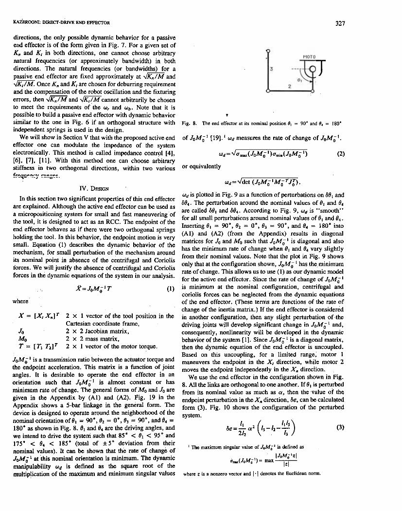
directions, the only possible dynamic behavior for a passiveend effector is of the form given in Fig. 7. For a given set ofKn and K1 in both directions, one cannot choose arbitrarynatural frequencies (or approximately bandwidth) in bothdirections. The natural frequencies (or bandwidths) for apassive end effector are fixed approximately at .JK;:1M and~ Once Kn and K1 are chosen for deburring requirementand the compensation of the robot oscillation and the fixturingerrors, then.JK;:1M and ~7M" cannot arbitrarily be chosento meet the requirements of the (AI, and cub. Note that it ispossible to build a passive end effector with dynamic behavior 'fsimilar to the one in Fig. 6 if an orthogonal structure with Fig. 8. The end effector at its nominal position 8, = 90. and 8, = 180.independent springs is used in the design.

We will show in Section V that with the proposed active end of JoMa I [19).1 CUd measures the rate of change of JoMa I.

effector one can modulate the impedance of the systemelectronically. This method is called impedance control [4), cud=.,Jumax(JoMal)Umin(JoMal) (2)[6), [7), [11). With this method one can choose arbitrary .stiffness in two orthogonal directions, within two various or equIvalently

freollencv ranf!e~~ --J ~ ---0---

IV. DESIGN

In this section two significant properties of this end effectorare explained. Although the active end effector can be used asa micropositioning system for small and fast maneuvering ofthe tool, it is designed to act as an RCC. The endpoint of theend effector behaves as if there were two orthogonal springsholding the tool. In this behavior, the endpoint motion is verysmall. Equation (1) describes the dynamic behavior of themechanism, for small perturbation of the mechanism aroundits nominal point in absence of the, centrifugal and Coriolisforces. We will justify the absence of centrifugal and Coriolisforces in the dynamic equations of the system in our analysis.

..-I." X=JoMo T (1)

where

X = [XI Xn] T 2 X 1 vector of the tool position in the

Cartesian coordinate frame,Jo 2 x 2 Jacobian matrix,Mo 2 x 2 mass matrix,T = [T1 T 2] T 2 x 1 vector of the motor torque.

JoM.)". is a transmission ratio between the actuator torque andthe endpoint acceleration. This matrix is a function of jointangles. It is desirable to operate the end effector in anorientation such that JoM.)" I is almost constant or has

minimum rate of change. The general forms of Mo and Jo aregiven in the Appendix by (AI) and (A2). Fig. 19 in theAppendix shows a 5-bar linkage in the general form. Thedevice is designed to operate around the neighborhood of thenominal orientation of 8. = 9()°, 82 = 00, 8) = 9()°, and 84 =1800 as shown in Fig. 8.8. and 84 are the driving angles, andwe intend to drive the system such that 850 < 8. < 950 and1750 < 84 < 1850 (total of :t5° deviation from theirnominal values). It can be shown that the rate of change ofJoM.)". at this nominal orientation is minimum. The dynamicmanipulability (o1d is defined as the square root of themultiplication of the maximum and minimum singular values

II ( Ills oe=- az Is-/z--

2/z 13(3)

I The maximum singular value of JoMo' is defined as

-I -IJoMolzl11_(JoMo )- max Izi

where z is a nonzero vector and 1.\ denotes the Euclidean nonn.

---\~el~

(Ald=Ydet (JoMo.MoTJf).

(AId is plotted in Fig. 9 as a function of perturbations on 08. and084. The perturbation around the nominal values of 8. and 84are called 08. and 084. According to Fig. 9, (AId is "smooth"for all small perturbations around nominal values of 8. and 84.Inserting 8. = 90°,82 = 0°,8) = 90°, and 84 = 180° into

(AI) and (A2) (from the Appendix) results in diagonalmatrices for Jo and Mo such that JoMo. is diagonal and alsohas the minimum rate of change when 8. and 84 vary slightlyfrom their nominal values. Note that the plot in Fig. 9 showsonly that at the configuration shown, JoMo. has the minimumrate of change. This allows us to use (1) as our dynamic modelfor the active end effector. Since the rate of change of JoM 0 .

is minimum at the nominal configuration, centrifugal andcoriolis forces can be neglected from the dynamic equationsof the end effector. (These terms are functions of the rate ofchange of the inertia matrix.) If the end effector is consideredin another configuration, then any slight perturbation of thedriving joints will develop significant change in JoMo. and,consequently, nonlinearity will be developed in the dynamicbehavior of the system [1]. Since JoMo. is a diagonal matrix,then the dynamic equation of the end effector is uncoupled.Based on this uncoupling, for a limited range, motor 1maneuvers the endpoint in the X, direction, while motor 2moves the endpoint independently in the Xn direction.

We use the end effector in the configuration shown in Fig.8. All the links are orthogonal to one another. If 8. is perturbedfrom its nominal value as much as a, then the value of theendpoint perturbation in the Xn direction, De, can be calcul~tedform (3). Fig. 10 shows the configuration of the perturbed

system.

,;~

~i~rott!

328 IEEE JOURNAL OF ROBOTICS AND AUTOMATION, YOLo 4, NO.3; JUNE 1988

."'.

3'-''-.,:~

V. ELECTRONIC COMPUANCY (IMPEDANCE CONTROL)

First we frame the controller design objectives by a set ofmeaningful mathematical terms; then we give a summary ofthe controller design method to d,evelop compliancy for linearsystcms. The complete description of the control method todevelop electronic compliancy (impedance control) for amulti-degree-of-freedom nonlinear manipulative system isgiven in [9] and [11].

The controller design objective is to provide a stabilizingdynamic compensator for the system such that the ratio of theposition of the endpoint of the end effector to an interactionforce is constant within a given operating frequency range.(The very general definition is given in [6] and [7].) The abovestatement can be mathematically expressed by (5).

~"elFig. 9. Dynamic manipulability as a function of 00. and 00..

~ LO-,MOTOR 2 MOTOR 1

)TL.

r-::\-"-

Tof(jCJJ) = KoX(jCJJ), (5)for all 0«01«010

l3

rx-..(+ XI~

~o-

~

",I:~!iri;'oi:

_L2--!Xn., '(5 ~

Fig. 10. The S-bar mechanism with small deflection of a.

For Oe = 0, the following equality must be satisfied:

1./5Is-h=- .(4)

4

By satisfying (4), we choose the lengths of the mechanismsuch that the endpoint of the end effector always moves alongthe X, axis for small value of a(a < :!: 5 O). This configurationis an application of the well-known Watts [12] straight linemechanism. This property is attractive for deburring purposes.According to [8], [10], the end effector must be very stiff inthe direction normal to the part and compliant in the directiontangential to the part. Once the grinder encounters a burr,motor 1, which is responsible for motion in the X, direction,moves the tool backward to decrease the amount of the force.In the deburring process, motor 1 constantly moves theendpoint back and forth in the X, direction. If (4) isguaranteed, then the motion of the endpoint in the X, directiondoes not affect the motion of the tool in the Xn direction. Thefollowing constraints are sufficient to result in the exactlengths of the mechanism:

.Equation (4) must be satisfied.

.For simplicity in design and construction, I. = 14 and4 = h.

.10 = 3 in (each actuator has 1.375-in radius).

.14 must be such that if 084 = 5°, the amount of motion inthe Xn direction is 0.15 in.

-~, ;

, '~!i;,, to..

::.t:H;

"fJ11i'~'!~~~1.1;'~1

(~~!\.' ~\ ~, " ,;, , ,\

\:11~!

The above five constraints are sufficient conditions to acquirethe lengths of the five links. Using the triangle equality andsome algebra, the following lengths are calculated: 10 = 3 in,11= O.906in,h = 1.917 in, 13 = 1.917in, and 14 = Q.906in.

where

of(j,,,) 2 x 1 vector of the deviation of the interactionforces from their equilibrium value in the globalCartesian coordinate frame;

oX(j",) 2 X 1 vector of the deviation of the endpointposition from the nominal point in the globalCartesian coordinate frame;

K 2 x 2 real-valued, nonsingular diagonal stiffnessmatrix with constant members;

"'0 bandwidth (frequency range of operation);j complex number notation, -r:-T:

The stiffness matrix is the designer's choice which, dependingon the application, contains different values for each direction.By specifying K, the designer governs the behavior of the endeffector in constrained maneuvers. Large elements of the Kmatrix imply large interaction forces and torques. Smallmembers of the K t:natrix allow for a considerable amount ofmotion in the end effector in response to interaction forces.Even though a diagonal stiffness matrix is appealing for thepurpose of static uncoupling, the K matrix in general is notrestricted to any structure.

Mechanical systems are not generally responsive to externalforces at high frequencies. As the frequency increases, theeffect of the feedback disappears gradually (depending on thetype of controller used), until the inertia of the systemdominates its overall motion. Therefore, depending on thedynamics of the system, (5) may not hold for a wide frequencyrange. It is necessary to consider, the specification of "'0 as thesecond item of interest. In other words, two independentissues are addressed by (5): first, a simple relationshipbetween of(j,,,) and oXU",); second, the frequency range ofoperation "'0' such that (5) holds true. Besides choosing anappropriate stiffness matrix K, and a viable "'0' a designermust also guarantee the stability of the closed-loop system. Insummary, we are looking for a dynamic behavior for themanipulative system that resembles the dynamic behaviorshown in Fig. 6.

We consider the architecture of Fig. 11 as the closed-loopcontrol system for the end effector. The detailed description ofeach operator in Fig. 11 is given in [9] and [11]. Since the

329KAZEROONl: DIRECT-DRIVE END EFFECTOR

dynamic behavior of the end effector in the neighborhood ofits operating point is linear, all the operators in Fig. II areconsidered transfer function matrices. In the general approachfor development of compliancy in [11], E, G, H, and S arenonlinear operators. G is the transfer function matrix thatrepresents the dynamic behavior of the manipulative system(end effector in our case) with a positioning controller. Theinput to G is the vector of input trajectory e. The fact that mostmanipulative systems have some kind of positioning control-lers is the motivation behind our approach. One can use a greatnumber of methodologies for the development of the robustpositioning controllers [14], [15], [18]. G can be calculatedexperimentally or analytically. Note that G is approximatelyequal to the unity matrix for the frequencies within itsbandwidth. S is the sensitivity transfer function matrix. Srepresents the relationship between the external force on theendpoint of the end effector and the endpoint motion. Thismotion is due to either structural compliance in the end-effector mechanism or the positioning controller compliance.For a good positioning system S is quite "small." (The notionof "small" can be regarded in the singular value sense when Sis a transfer function matrix. Lp-norm [18], [17] can beconsidered to show the size of S in the nonlinear case.) Erepresents the dynamic behavior of the environment. Readerscan be convinced of the role of E by analyzing the relationshipof the force and displacement of a spring as a simple model ofthe environment. H is the compensator to be designed. Theinput to this compensator is the contact force. The compensa-tor output signal is being subtracted from the vector of inputcommand r, resulting in the error signal e, as the inputtrajectory for the robot manipulator. r is the input commandvecto)" in the global coordinate frame which is used differentlyfor the two categories of maneuvers; as a trajectory commandto move the endpoint in unconstrained space and as acommand to shape the contact force in the constrained space.When the manipulative system and environment are in contact,then the value of the contact force and the endpoint positionare given by (6) and (7).

F=E(I+SE+GHE)-I(Gr-Xo) (6)

X=(I+SE+GHE)-I(Gr-Xo). (7)

The general goal is to choose a class of compensator H toshape the impedance of the system E(I + SE + GHE)-IGin (6). When the system is not in contact with the environment,the actual position of the endpoint is equal to the inputtrajectory command within the bandwidth of G. {Note that- G

Fig. 11.

1for all '" E (0, (XI)

(8)

F=(S+GH)-'Xo. (9)

Since G IS a unity matrix for all (11 E (0, (110), the value of thecontact force F, within the bandwidth of the system (0, (110)'can be approximated by (10).

F=(S+H)-IXo,

By knowing 8 and choosing H, one can shape the contactforce. The value of (8 + H) within (0, CJ)0) is the designer'schoice and, depending on the task, it can have various valuesin different directions. A large value for (8 + H) within (0,"'0) develops a compliant system while a small (8 + H)generates a stiff system. If H is chosen such that (8 + H) is"large" in the singular value sense at high frequencies, thenthe contact force in response to high-frequency components ofr will be small. (S + H) -1 is similar to the stiffness matrix, Kwhich is defined by (5). By selecting the value of Hand

is approximately equal to unity matrix within its bandwidth.)When the system is in contact with the environment, then thecontact force follows r according to (6). We do not commandany setpoint for force as we do in admittance control [13],[21]. This method is called Impedance Control [4], [6], [7]because it accepts a position vector as input and reflects a forcevector as output. There is no hardware or software switch inthe control system when the robot travels from unconstrainedspace to constrained space. The feedback loop on the contactforce closes naturally when the robot encounters the environ-ment. When the system is in contact with the environment,then the contact force is a function of r according to (6).

The compensator H must also guarantee the stability of theclosed-loop system of Fig. II. The general nonlinear suffic-ient condition for stability of the closed-loop system is given in[9] and [11]. The sufficient condition for stability of thelinearly tr~ated systems is given by inequality (8).

0' (H ) ~ -~ -'max O'max(E(SE+ln)-IG)' f.

If H is chosen outside of this class, instability andconsequent separation may occur. Inequality (8) is a sufficientcondition for stability. If inequality (8) is not satisfied, noconclusion on the stability of the system can be reached.Inequality (8) reveals some facts about the size of H. Thesmaller the sensitivity S, the smaller H must be chosen. Also,from inequality (8), the more rigid the environment, thesmaller H must be chosen. In the "ideal case," no H can be"found to allow a perfect positioning system (S = 0) to interactwith an infinitely rigid environment (E = 00).

In most manufacturing tasks such as robotic deburring, theendpoint of the manipulative system is in contact with a verystiff environment. We are interested in a particular case whenr = O. Suppose the environment is being moved into the endeffector or the end effector is being moved into the environ-ment as much as Xo. The relation between the c:,ontact forceand the endpoint deflection is given by (9) if E approaches 00in the singular value sense.

, ."I---/ ,

-.1 -

--'1:;

.",- -' -~ --' for all '" E (0, "'0). (.0)

,- J

"""..aJt:

,j

~:330 IEEE JOURNAL OF ROBOTICS AND AUTOMATION, YOLo 4, NO.3, JUNE 1988

knowledge of 8 one can select the members of H such that (8 directions in the Cartesian coordinate frame. The force+ H)-I of (10) meets the deburring requirements as given by transducer is preloaded at the endpoint of the end effector by a(5). It is shown in [9] and [II] that the stability criterion for clamping screw as shown in Fig. 3. The resolution of the forceinteraction with a very rigid environment is given by inequal- transducer is 2.2 X 10-3 lbf. The stiffness of the forceity (11). transducer in each measuring direction is about 1,5 X 1091bf/

in.1

O"max{H) ~ -for all (AI E {O, (XI). (II)

It is clear that if the environment is very rigid, then one mustchoose a very s~all H to satisfy the stability of the systemwhen S is "small." (A good positioning system has "small"S.) Since G is a unity matrix for all (AI E (O, (Ala), the bound forH, for a rigid environment and a "small" stiffness, is given

by inequality (12).f;

O"max{H) ~ O"min{S), for all (AI E {O, (Alo). (12)

If S is zero, then no H can be obtained to stabilize the system.In other words, to stabilize the system of the very rigidenvironment and the end effector, there must be a minimumcompliancy in the end effector.

In general, for stability of the environment and a robot takenas a whole, there must be some initial compliancy either in therobot or in the environment. The initial compliancy in therobot can be obtained by a nonzero sensitivity function or apassive compliant element such as an RCC (Remote CenterCompliance). Practitioners always observed that the system ofa robot and a stiff environment can always be stabilized when acompliant element (e.g., piece of rubber or an RCC) isinstalled between the robot and environment. One can alsostabilize the system of robot and environment by increasingthe robot sensitivity function. In many commercial manipula.,tors the sensitivity of the robot manipulators can be increasedb~ decreasing the gain of each actuator positioning loop. Thisal~o results in a narrower bandwidth (slow response in theunconstrained maneuvering) for the robot positioning system.

I ,

Urnax(S-IG)'

fi!

VI. EXPERIMENTS,Two sets of experiments are described here to present the

dynamic behavior of t~e end effector in constrained andunconstrained maneuvering. In Section VI-A, the experimen-tal frequency response ?f the transfer function matrix G andthe sensitivity transfer function matrix 8 are given. The valuesof G and 8 are necessary to estimate the stability bound on H.Section VI-B demonstrates the endpoint impedance (8 +H)-I and the uncoup1ed time-domain closed-loop dynamicbehavior of the end effa:tor in the constrained and uncon-strained maneuvering. T.be cO;ntrol architecture of Fig. 11 isused to control the syst~m.

Two brushless dc rpotors are used to power the two degreesof freedom of the en4 effector. The continuous stall torque andpeak t<>;rque are 5 lpf-in and 20 lbf-in at 2.25 and 6.7 A,respectively. Motors are driven by two PWM amplifiers. Theampufier has 7.5-A continuous output current. Both motorsare equipped with resolvers that provide 12-bit orientation dataarid an analog velocity feedback signal with resolution of0.019 V/rad/s. A two-component piezoelectric force trans-ducer and a charge amplifier are used to; measure forces in two

B. The Closed-Loop Dynamic Behavior of the EndEffector

Frequency-domain and time-domain methods have beenused to describe the dynamic behavior of the closed-loopsystem. Section VI-BI is devoted to verifying experimentallythe model of the endpoint compliancy in both directions whenan H is designed to close the loop as shown in Fig. II.

1) The Endpoint Compliancy: The nature of compliancyfor the end effector is given by (9). H was chosen such that (S+ H) -J in each direction is equal to the desired' stiffness

given by (5). H must also guarantee the stability of the closed-loop system. The stability criterion for a one-degree-of-freedom system is given by inequality (13).

IHOI<I(S+I/E)I. forall",E(O.~) (13)

where 1 .I denotes the magnitude of a transfer function. Sincein many cases 0 = I for all 0 < '" < "'0. then H must bechosen such that the following inequality is satisfied:

IHI < I(S+ l/E)I. for all", E (0. "'0)' (14)

Inequality (14) shows that the more rigid the environment. thesmaller H must be chosen to guarantee the stability of the i~n)t f ; " 11"

IJ~;~' ~

p:; !,j;!:

Since the dynamic behavior of the end effector in twodirections is uncoupled, matrices E, S, G, and H of Fig. IIare diagonal. Each motor of the end effector was treatedseparately and a control loop similar to the one in Fig. 11 wasdesigned for each motor.

A. Experimental and Theoretical Values of G and S

In this set of experiments, the position transfer functionmatrix G and the sensitivity transfer function S are measured.Fig. 12 shows the analytical and experimental values of G fortwo orthogonal directions. For measuring G, a series ofsinusoidal commands with frequencies within 15 Hz wereimposed on each motor.

The amplitude of orientation of each motor was measured ateach frequency. The ratio of the rotation of the motor to theinput command represents the magnitude of G at eachfrequency. For measurement of the sensitivity transfer func-tion matrix, the input excitation was supplied by the rotation ofan eccentric mass mounted on the tool bit. Fig. 13 shows theexperimental setup for measurement of S. The rotating massexerts a centerifugal, sinusoidal force on the tool bit. Thefrequency of the imposed force is equal to the frequency ofrotation of the mass. By varying the frequency of the rotationof the mass, one can vary the frequency of the imposed forceon the end effector. Fig. 14 depicts the sensitivity transferfunction. The values of the sensitivity transfer functions alongthe normal and tangential directions, within their bandwidths,are 0.7 in/lbfand 0.197 in/lbf, respectively.

---

KAZEROONI: DIRECT -DRIVE END EFFECTOR 331

In.. I -..,

.: D~t~

-: SlmuL~tlon~ 16)(IU"'I/ 6f.lj..,JI /

/16)(.U..,I/6f.U..,11

db In/Lbf

.01

Fig. 15.

100 1000r~d/sec

The endpoint admittance (l/impedance).

G In K. direction

db

-10 .: Doto-: Simulotion

-1~

I 10 100red/sac

Fig. 12. The position transfer function G.

Fig. 13,

+xn

The experimental setup for measurement of the sensitivity transferfunction.

x.dlrectlonK'

KI directionIn/lbf

.:Doto

-:Slmulatlon.DII I ID IDO 1000

rod/S8C

Fig. 14. The sensitivity transfer function S.

endpoint compliancy. The dynamic behavior of Fig. 15 can becompared with the desired dynamic response for deburringgiven by Fig. 6.

2) Uncoupling of the Contact Forces: In this set ofexperiments, the whole end effector was moved in twodifferent directions to encounter an edge of a part. Theobjective was to observe the uncoupled time-domain dynamicbehavior of the end effector when the end effector is in contactwith the hard environment. The controller was designedaccording to [11] such that KI and Kn are 0.32 and 4.0 Ib/in,respectively. First, the end effector was moved 0.5 in beyondthe edge of the part in the Xn direction. Fig. 8 shows theschematics of the setup.

Fig. 16 shows the contact forces. The force in the Xndirection increases from zero to 2.0 Ibf while the force in theXI direction remains at zero. Next, the end effector was moved0.5 in beyond the edge of the part in the XI direction. Fig. 17shows the contact forces. The force in the X, directionincreases from zero to 0.16 Ibf while the force in the Xndirection remains at zero. In both cases, the end effector wasmoved 0.5 in beyond the edge of the stiff wall. Since thestiffness of the end effector in the Xn direction is larger thanthe stiffness in the X, direction, the contact force in the Xndirection is larger than the contact force in the X, direction.

3) Uncoupling of the Motion: The objective was toobserve the uncoupled dynamic behavior of the end effector inunconstrained maneuvering of the end effector when (4) issatisfied. The endpoint of the end effector was ordered tomove in the X, direction. Fig. 18 shows the joint angles, 01 and0., of the end effector when 01 is accepting a step-wise motioncommand. O. remains at 180°. The plot shows the uncouplingof the joint angles in the closed-loop system.

Vll. SUMMARY AND CONCLUSION

An active end effector with controllable, compliant motion(Electronic Compliancy) has been designed, built, and testedfor robotic operations. The active end effector (unlike thepassive system) does not contain any spring or dampers. Thecompliancy in the active end effector is developed electroni-cally and therefore can be modulated by an on-line computer.The active end effector allows for compensation of the robot'sposition uncertainties from fixturing errors, robot programingresolution, and robot oscillations. This fully instrumented endeffector weighs only 5.05 lb and can be mounted at theendpoint of the commercial robot manipulator. Two state-of-the-art miniature actuators power the end effector directly.The high stiffness and light weight of the material used in the

closed-loop system. In the case of a rigid environment("large" E) and a "good" ~sitioning system, H must bechosen as a very small gain. The values for H along thenormal and tangential directions within their bandwidths are0.01 and 0.194 in/lbf, respectively. These values result in 0.39and 0.7 in/lbf for (S + H) within the bandwidth of thesystem. The values of(S + H) within its bandwidth representthe members of matrix K-I in (5). Fig. 15 shows theexperimental and theoretical values of the endpoint compli-ancy (Fig. 15 actually shows the endpoint admittance where itis reciprocal of the impedance in the linear case.) Theexperimental setup shown in Fig. 13 was used to measure the

~:,II!~'j;i1

332 IEEE JOURNAL OF ROBOllCS AND AUTOMAll0N, YOLo 4, NO.3, JUNE 1988

Fig. 16. Force in the X~ direction increases from zero to 2 Ibf.Fig. 19. The 5-bar linkage in the general form.

be represented by (AI)

J11 JI2

J21 J22Jo=

where

J11= -II sin (0.)+015 sin (OJ

J21=/1 COS (01)-015 COS (02)

J12= -his sin (OJ

J22 = bls cos (OV.

where

Mil =h +m2If+ jza2+ hC2+2x211 COS (01-02)am2

MI2 = hob + b COS (01 -02)x211 m2

+hcd+c cos (O4-0J)xJI4mJ

M21=M12

M22=2mJI4xJd cos (04 -OJ)+ hd2+ j4+mJI~+ jzb2.

a, b, c, and d are given below.system allows for a wide-bandwidth impedance control. Aminiature force cell measures the forces in two dimensions.The tool holder can maneuver a very light pneumatic grinderin a linear workspace of about 0.3 in X 0.3 in. Themeasurements taken on the mechanism are contact forces,angular velocities, and the orientation of the mechanism.Satisfying a kinematic constraint for this end effector allowsfor uncoupled dynamic behavior for a bounded range.

:~"

,t

[."t\[f:

I!,

a = II sin (fJl- fJ3)/(/2 sin (fJ2 -fJ3»

b=/4 sin (fJ4-fJ3)/(h sin (fJ2-fJ3»

c= II sin (fJl- fJ2)/(/3 sin (fJ2 -fJ3»

d= 14 sin (fJ4 -fJv/(/3 sin (fJ2 -fJ3».

REFERENCES

[I] H. Asada and K. Youcef-Toumi, "Analysis and design ofa direct drivearm with a five-bar-link parallel d~ive mechanism," ASME J.Dynamic Syst., Meas., Contr., vol. 106, no. 3, pp. 225-230, 1984.

[2] J. Bausch, B. Kramer, and H. Kazcrooni, "The development of thecompliant tool holders for robotic deburring," presented at the ASMEWinter Annual Meet., Anaheim, CA, Dec. 1986.

[3] S. H. Drake, "Using compliance in lieu of sensory feedback forautomatic assembly," presented at the IFAC Symp. on Information andControl Problems in Manufacturing Technology, Tokyo, Japan, 1977.

ApPENDIX

This Appendix is dedicated to deriving of the Jacobian andthe mass matrix of a general 5-bar linkage. In Fig. 19, h, fi,Xi, mi, and Oi represent the moment of the inertia relative to theendpoint, length, location of the center of mass, mass, and theorientation of each link for i = 1, 2, 3, and 4.

Using the standard method, the Jacobian of the linkage can

J{A.zEICOONI: DIRECf-DRIVE END EFFECfOR 333

(16] M. Vidyasagar, Non-Linear Systems Analysis. Englewood Cliffs,NJ: Prentice-Hall, 1978.

(17] C. A, Desoer and M. Vidyasagar, Feedback Systems: Input-OutputProperties. New York, NY: Academic Press, 1975.

[18] M. Vidyasagar and W. M. Spong, "RobJst non-linear control of robotmanipulators," presented at the IEEE Conf. on Decision and Control,Dec. 1985.

(19] T. Yoshikawa, "Dynamic manipulability of robot manipulators," J,Robotic Syst., vol. 2, no. I, 1985.

(20) P. C. Watson, "A multidimensional system analysis of the assemblyprocess as performed by a manipulator," in Proc. 1st Amer. RobotCon/. (Chicago, IL, 1976).

(21] D. E. Whitney, "Force-feedback control of manipulator fine mo-tions," ASME J. Dynamic Syst., Meas., Contr., June 1977.

H. Kazerooni was born in Tehran. Iran, in May1956. He received the M.S. degree in mechanicalengineering from the University of Wisconsin,Madison, in 1980, and the M.S.M.E. and Sc.D.degrees in mechanical engineering from the Man-Machine Systems Laboratory of the MassachusettsInstitute of Technology, Cambridge, in 1982 and1984, respectively.

From 1984 to 1985, he was with the Laboratoryof Manufacturing and Productivity at the Massachu-~ setls Institute of Technology as a Post Doctoral

Fellow. He is currently Assistant Professor in Mechanical EngineeringDepartment at the University of Minnesota, Minneapolis.

[4] N. Hogan, "Impedance control: An approach to manipulation, Part I:Theory, Part 2: Implementation, Part 3: Applications," A8ME J.Dynamic 8yst.. Meas.. Contr., 1985.

[5] R. L. Hollis, "A planar XY robotic fine positioning device," in Proc.IEEE Int. Con/. on Robotics and Automation (St. Louis, MO, Mar.1985).

[6] H. Kazerooni, P. K. Houpt, and T. B. Sheridan, "Fundamentals ofrobust compliant motion for manipulators," IEEE J. RoboticsAutomat., vol. RA-2, no. 2, pp. June 1986.

[7] -,"A design method for robust compliant motion of manipula-tors," IEEE J. Robotics Automat., vol. RA-2, no. 2, pp. June 1986.

[8] H. Kazerooni, J. J. Bausch, and B. Kramer, "An approach toautomated deburring by robot manipulators," A8ME J. Dynamic8yst., Meas.. Contr., Dec. 1986.

[9] H. Kazerooni, "On the stability of the robot compliant motioncontrol," in Proc. 16th IEEE Con}: on Decision and Control (LosAngeles, CA, Dec. 1987).

[10] -,"Automated robotic deburring using electronic compliancy;impedance control," in Proc. IEEE Int. Con/. on Robotics andAutomation (Raleigh, NC, Mar. 1987).

[II] -, "Non-linear robust impedance control for robot manipulators,"in Proc. IEEE Int. Con}: on Robotics and Automation (Raleigh,NC, Apr. 1987).

[12] S. Rappaport, "Five-bar linkage for straight line motion," ProductEng., Oct. 1959.

[13] M. H. Raibert and J. J. Craig, "Hybrid position/force control ofmanipulators," A8ME J. Dynamic 8yst., Meas., Contr., June 1981.

[14] J. J. Slotine, "Sliding controller design for non-linear systems," Int.J. Contr., vol. 40, no. 2, 1984.

[15] -, "The robust control of of robot manipulators," Int. J. Robot.Res., vol. 4, no. 2, 1985.