Bilateral Filtering for Gray and Color Images

C. Tomasi�

R. Manduchi

Computer Science Department Interactive Media GroupStanford University Apple Computer, Inc.Stanford, CA 94305 Cupertino, CA 95014

tomasi@cs.stanford.edu manduchi@apple.com

Abstract

Proceedings of the 1998 IEEE InternationalConference on Computer Vision, Bombay,India

Bilateral filtering smooths images while preservingedges, by means of a nonlinear combination of nearbyimage values. The method is noniterative, local, and sim-ple. It combines gray levels or colors based on both theirgeometric closeness and their photometric similarity, andprefers near values to distant values in both domain andrange. In contrast with filters that operate on the threebands of a color image separately, a bilateral filter can en-force the perceptual metric underlying the CIE-Lab colorspace, and smooth colors and preserve edges in a waythat is tuned to human perception. Also, in contrast withstandard filtering, bilateral filtering produces no phantomcolors along edges in color images, and reduces phantomcolors where they appear in the original image.

1 IntroductionFiltering is perhaps the most fundamental operation of

image processing and computer vision. In the broadestsense of the term “filtering,” the value of the filtered imageat a given location is a function of the values of the in-put image in a small neighborhood of the same location. Inparticular, Gaussian low-pass filtering computes a weightedaverage of pixel values in the neighborhood, in which, theweights decrease with distance from the neighborhood cen-ter. Although formal and quantitative explanations of thisweight fall-off can be given [11], the intuitionis that imagestypically vary slowly over space, so near pixels are likelyto have similar values, and it is therefore appropriate toaverage them together. The noise values that corrupt thesenearby pixels are mutually less correlated than the signalvalues, so noise is averaged away while signal is preserved.

The assumption of slow spatial variations fails at edges,which are consequently blurred by low-pass filtering. Manyefforts have been devoted to reducing this undesired effect[1, 2, 3, 4, 5, 6, 7, 8, 9, 10, 12, 13, 14, 15, 17]. How can

�

Supported by NSF grant IRI-9506064 and DoD grants DAAH04-94-G-0284 and DAAH04-96-1-0007, and by a gift from the Charles LeePowell foundation.

we prevent averaging across edges, while still averagingwithin smooth regions? Anisotropic diffusion [12, 14] is apopular answer: local image variation is measured at everypoint, and pixel values are averaged from neighborhoodswhose size and shape depend on local variation. Diffusionmethods average over extended regions by solving partialdifferential equations, and are therefore inherently iterative.Iteration may raise issues of stability and, depending on thecomputational architecture, efficiency. Other approachesare reviewed in section 6.

In this paper, we propose a noniterative scheme for edgepreserving smoothing that is noniterative and simple. Al-though we claims no correlation with neurophysiologicalobservations, we point out that our scheme could be imple-mented by a single layer of neuron-like devices that performtheir operation once per image.

Furthermore, our scheme allows explicit enforcementof any desired notion of photometric distance. This isparticularly important for filtering color images. If thethree bands of color images are filtered separately fromone another, colors are corrupted close to image edges. Infact, different bands have different levels of contrast, andthey are smoothed differently. Separate smoothing perturbsthe balance of colors, and unexpected color combinationsappear. Bilateral filters, on the other hand, can operate onthe three bands at once, and can be told explicitly, so tospeak, which colors are similar and which are not. Onlyperceptually similar colors are then averaged together, andthe artifacts mentioned above disappear.

The idea underlying bilateral filtering is to do in therange of an image what traditional filters do in its domain.Two pixels can be close to one another, that is, occupynearby spatial location, or they can be similar to one an-other, that is, have nearby values, possibly in a perceptuallymeaningful fashion. Closeness refers to vicinity in the do-main, similarity to vicinity in the range. Traditional filter-ing is domain filtering, and enforces closeness by weighingpixel values with coefficients that fall off with distance.Similarly, we define range filtering, which averages image

values with weights that decay with dissimilarity. Rangefilters are nonlinear because their weights depend on imageintensity or color. Computationally, they are no more com-plex than standard nonseparable filters. Most importantly,they preserve edges, as we show in section 4.

Spatial locality is still an essential notion. In fact, weshow that range filtering by itself merely distorts an image’scolor map. We then combine range and domain filtering,and show that the combination is much more interesting.We denote teh combined filtering as bilateral filtering.

Since bilateral filters assume an explicit notion of dis-tance in the domain and in the range of the image function,they can be applied to any function for which these twodistances can be defined. In particular, bilateral filters canbe applied to color images just as easily as they are appliedto black-and-white ones. The CIE-Lab color space [16]endows the space of colors with a perceptually meaningfulmeasure of color similarity, in which short Euclidean dis-tances correlate strongly with human color discriminationperformance [16]. Thus, if we use this metric in our bilat-eral filter, images are smoothed and edges are preserved in away that is tuned to human performance. Only perceptuallysimilar colors are averaged together, and only perceptuallyvisible edges are preserved.

In the following section, we formalize the notion ofbilateral filtering. Section 3 analyzes range filtering inisolation. Sections 4 and 5 show experiments for black-and-white and color images, respectively. Relations withprevious work are discussed in section 6, and ideas forfurther exploration are summarized in section 7.

2 The IdeaA low-pass domain filter applied to image f

�x � produces

an output image defined as follows:

h�x �������� � x � � �� �

���� � f

��� ��� ����� x ��� � (1)

where � ����� x � measures the geometric closeness betweenthe neighborhood center x and a nearby point

�. The bold

font for f and h emphasizes the fact that both input andoutput images may be multiband. If low-pass filtering is topreserve the dc component of low-pass signals we obtain

� � x ��� � �� �� �� � �

�����x ��� ��� (2)

If the filter is shift-invariant, � ����� x � is only a function ofthe vector difference

���x, and � is constant.

Range filtering is similarly defined:

h�x ����� ���� � x � � �� �

� �� � f��� ��� � f ��� � � f � x ����� � (3)

except that now � � f ��� � � f � x ��� measures the photometric sim-ilarity between the pixel at the neighborhood center x and

that of a nearby point�. Thus, the similarity function �

operates in the range of the image function f, while thecloseness function � operates in the domain of f. The nor-malization constant (2) is replaced by

� � � x ��� � �� �� �� � �

�f��� � � f � x ����� ��� (4)

Contrary to what occurs with the closeness function � , thenormalization for the similarity function � depends on theimage f. We say that the similarity function � is unbiasedif it depends only on the difference f

��� � � f�x � .

The spatial distributionof image intensities plays no rolein range filtering taken by itself. Combining intensitiesfrom the entire image, however, makes little sense, sinceimage values far away from x ought not to affect the finalvalue at x. In addition, section 3 shows that range filteringby itself merely changes the color map of an image, andis therefore of little use. The appropriate solution is tocombine domain and range filtering, thereby enforcing bothgeometric and photometric locality. Combined filteringcanbe described as follows:

h�x �!�"� �� � x � ���� �

� �� � f

��� �#� ����� x �#� � f ��� � � f � x ����� � (5)

with the normalization

� � x ��� ���� ����� � �

�����x ��� � f ��� � � f � x �#��� �$� (6)

Combined domain and range filtering will be denotedas bilateral filtering. It replaces the pixel value at x withan average of similar and nearby pixel values. In smoothregions, pixel values in a small neighborhood are similar toeach other, and the normalized similarity function � �� � isclose to one. As a consequence, the bilateral filter acts es-sentially as a standard domain filter, and averages away thesmall, weakly correlated differences between pixel valuescaused by noise. Consider now a sharp boundary betweena dark and a bright region, as in figure 1 (a). When thebilateral filter is centered, say, on a pixel on the bright sideof the boundary, the similarity function � assumes valuesclose to one for pixels on the same side, and close to zero forpixels on the dark side. The similarity function is shown infigure 1 (b) for a %'&)(*%+& filter support centered two pixelsto the right of the step in figure 1 (a). The normalizationterm � � x � ensures that the weights for all the pixels add upto one. As a result, the filter replaces the bright pixel at thecenter by an average of the bright pixels in its vicinity, andessentially ignores the dark pixels. Conversely, when thefilter is centered on a dark pixel, the bright pixels are ig-nored instead. Thus, as shown in figure 1 (c), good filteringbehavior is achieved at the boundaries, thanks to the do-main component of the filter, and crisp edges are preservedat the same time, thanks to the range component.

(a) (b) (c)

Figure 1: (a) A 100-gray-level step perturbed by Gaussian noise with ������� gray levels. (b) Combined similarity weights ����� x ���� f �� �� f � x � for a���������neighborhood centered two pixels to the right of the step in (a). The range component effectively suppresses the pixels on the dark side. (c) The

step in (a) after bilateral filtering with ��������� gray levels and ��� ��� pixels.

2.1 Example: the Gaussian CaseA simple and important case of bilateral filtering is

shift-invariant Gaussian filtering, in which both the close-ness function � ����� x � and the similarity function � ��!�� f � areGaussian functions of the Euclidean distance between theirarguments. More specifically, � is radially symmetric

� ����� x ���#" �%$&('*)�+ ,�- .�/0 )21 &where � ����� x �!� � ��� � x ���43 ��� x 3is the Euclidean distance between

�and x. The similarity

function � is perfectly analogous to � :� ����� x ���5" �6$& '87 + 9:+ ,�/;- 9:+ .�/</0>= 1 &

where ? ��!��f ��� ? ��! � f ���@3 ! � f 3

is a suitable measure of distance between the two intensityvalues

!and f. In the scalar case, this may be simply the

absolute difference of the pixel difference or, since noiseincreases with image intensity, an intensity-dependent ver-sion of it. A particularly interesting example for the vectorcase is given in section 5.

The geometric spread A in the domain is chosen basedon the desired amount of low-pass filtering. A large A blurs more, that is, it combines values from more distantimage locations. Also, if an image is scaled up or down, A must be adjusted accordingly in order to obtain equivalentresults. Similarly, the photometric spread A � in the imagerange is set to achieve the desired amount of combinationof pixel values. Loosely speaking, pixels with values muchcloser to each other than A � are mixed together and valuesmuch more distant than A � are not. If the image is amplifiedor attenuated, A � must be adjusted accordingly in order toleave the results unchanged.

Just as this form of domain filtering is shift-invariant,the Gaussian range filter introduced above is insensitive tooverall additive changes of image intensity, and is therefore

unbiased: if filtering f�x � produces h

�x � , then the same filter

applied to f�x �CB a yields h

�x �CB a, since

? �f��� �DB a

�f�x �DB

a ��� ? � f ��� �(B a� �

f�x �(B a �#��� ? � f ��� � � f

�x �#� . Of course,

the range filter is shift-invariant as well, as can be easilyverified from expressions (3) and (4).

3 Range Versus Bilateral FilteringIn the previous section we combined range filtering with

domain filtering to produce bilateral filters. We now showthat this combination is essential. For notational simplicity,we limit our discussion to black-and-white images, butanalogous results apply to multiband images as well. Themain point of this section is that range filtering by itselfmerely modifies the gray map of the image it is applied to.This is a direct consequence of the fact that a range filterhas no notion of space.

Let E ��! � be the frequency distribution of gray levels inthe input image. In the discrete case, E ��! � is the gray levelhistogram:

!is typically an integer between F and %�GHG , andE ��! � is the fraction of image pixels that have a gray value

of!

. In the continuous case, E ��! ��� ! is the fraction ofimage area whose gray values are between

!and

! B � ! .For notational consistency, we continue our discussion inthe continuous case, as in the previous section.

Simple manipulation, omitted for lack of space, showsthat expressions (3) and (4) for the range filter can be com-bined into the following:

I � � �J !LK ��!���M ��� ! (7)

where K ��!���M ��� � ��!��NM �(E ��! �O��J � ��!��NM �(E ��! ��� !independently of the position x. Equation (7) shows rangefiltering to be a simple transformation of gray levels. Themapping kernel

K ��!���M � is a density function, in the sensethat it is nonnegative and has unit integral. It is equalto the histogram E ��! � weighted by the similarity function� centered at

Mand normalized to unit area. Since

Kis

formally a density function, equation (7) represents a mean.We can therefore conclude with the following result:

Range filtering merely transforms the gray mapof the input image. The transformed gray value isequal to the mean of the input’s histogram valuesaround the input gray level

M, weighted by the

range similarity function � centered atM

.

It is useful to analyze the nature of this gray map trans-formation in view of our discussion of bilateral filtering.Specifically, we want to show that

Range filtering compresses unimodal histograms.

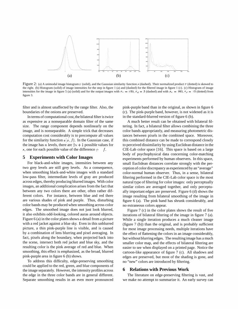
In fact, suppose that the histogram E ��M � of the inputimage is a single-mode curve as in figure 2 (a), and consideran input value of

Mlocated on either side of this bell curve.

Since the symmetric similarity function � is centered atM

,on the rising flank of the histogram, the product ��E producesa skewed density

K ��!���M � . On the left side of the bellK

isskewed to the right, and vice versa. Since the transformedvalue

Iis the mean of this skewed density, we have

I � Mon the left side and

I�� Mon the right side. Thus, the

flanks of the histogram are compressed together.At first, the result that range filtering is a simple remap-

ping of the gray map seems to make range filtering ratheruseless. Things are very different, however, when range fil-tering is combined with domain filtering to yield bilateralfiltering, as shown in equations (5) and (6). In fact, considerfirst a domain closeness function � that is constant withina window centered at x, and is zero elsewhere. Then, thebilateral filter is simply a range filter applied to the window.The filtered image is still the result of a local remappingof the gray map, but a very interesting one, because theremapping is different at different points in the image.

For instance, the solid curve in figure 2 (b) shows thehistogram of the step image of figure 1 (a). This histogramis bimodal, and its two lobes are sufficiently separate toallow us to apply the compression result above to eachlobe. The dashed line in figure 2 (b) shows the effect ofbilateral filtering on the histogram. The compression effectis obvious, and corresponds to the separate smoothing ofthe light and dark sides, shown in figure 1 (c). Similarconsiderations apply when the closeness function has aprofile other than constant, as for instance the Gaussianprofile shown in section 2, which emphasizes points thatare closer to the center of the window.

4 Experiments with Black-and-White Im-ages

In this section we analyze the performance of bilateralfilters on black-and-white images. Figure 5 (a) and 5 (b) inthe color plates show the potential of bilateral filtering for

the removal of texture. Some amount of gray-level quan-tization can be seen in figure 5 (b), but this is caused bythe printing process, not by the filter. The picture “sim-plification” illustrated by figure 5 (b) can be useful fordata reduction without loss of overall shape features in ap-plications such as image transmission, picture editing andmanipulation, image description for retrieval. Notice thatthe kitten’s whiskers, much thinner than the filter’s win-dow, remain crisp after filtering. The intensity values ofdark pixels are averaged together from both sides of thewhisker, while the bright pixels from the whisker itself areignored because of the range component of the filter. Con-versely, when the filter is centered somewhere on a whisker,only whisker pixel values are averaged together.

Figure 3 shows the effect of different values of the pa-rameters A and A � on the resulting image. Rows corre-spond to different amounts of domain filtering, columns todifferent amounts of range filtering. When the value of therange filtering constant A � is large (100 or 300) with respectto the overall range of values in the image (1 through 254),the range component of the filter has little effect for smallA : all pixel values in any given neighborhood have aboutthe same weight from range filtering, and the domain filteracts as a standard Gaussian filter. This effect can be seenin the last two columns of figure (3). For smaller valuesof the range filter parameter A � (10 or 30), range filteringdominates perceptually because it preserves edges.

However, for A ��� F , image detail that was removed bysmaller values of A reappears. This apparently paradoxicaleffect can be noticed in the last row of figure 3, and inparticularly dramatic form for A � ��� F�F , A ����F . Thisimage is crisper than that above it, although somewhat hazy.This is a consequence of the gray map transformation andhistogram compression results discussed in section 3. Infact, A ��� F is a very broad Gaussian, and the bilateralfilter becomes essentially a range filter. Since intensityvalues are simply remapped by a range filter, no loss ofdetail occurs. Furthermore, since a range filter compressesthe image histogram, the output image appears to be hazy.Figure 2 (c) shows the histograms for the input image andfor the two output images for A � ����F�F , A � & , and forA � ��� FHF , A ��� F . The compression effect is obvious.

Bilateral filtering with parameters A � & pixels andA � �5G�F intensity values is applied to the image in figure 4(a) to yield the image in figure 4 (b). Notice that most ofthe fine texture has been filtered away, and yet all contoursare as crisp as in the original image.

Figure 4 (c) shows a detail of figure 4 (a), and figure4 (d) shows the corresponding filtered version. The twoonions have assumed a graphics-like appearance, and thefine texture has gone. However, the overall shading ispreserved, because it is well within the band of the domain

f −40 −20 0 20 40 60 80 100 120 1400

200

400

600

800

1000

1200

0 50 100 150 200 250 3000

200

400

600

800

1000

1200

1400

(a) (b) (c)

Figure 2: (a) A unimodal image histogram � (solid), and the Gaussian similarity function � (dashed). Their normalized product � (dotted) is skewed tothe right. (b) Histogram (solid) of image intensities for the step in figure 1 (a) and (dashed) for the filtered image in figure 1 (c). (c) Histogram of imageintensities for the image in figure 5 (a) (solid) and for the output images with �H� ������� , ����� � (dashed) and with ����� �:��� , ��� � �:� (dotted) fromfigure 3.

filter and is almost unaffected by the range filter. Also, theboundaries of the onions are preserved.

In terms of computational cost, the bilateral filter is twiceas expensive as a nonseparable domain filter of the samesize. The range component depends nonlinearly on theimage, and is nonseparable. A simple trick that decreasescomputation cost considerably is to precompute all valuesfor the similarity function � ��!���M � . In the Gaussian case, ifthe image has � levels, there are % � B � possible values for� , one for each possible value of the difference

!$� M.

5 Experiments with Color ImagesFor black-and-white images, intensities between any

two grey levels are still grey levels. As a consequence,when smoothing black-and-white images with a standardlow-pass filter, intermediate levels of gray are producedacross edges, thereby producing blurred images. With colorimages, an additional complication arises from the fact thatbetween any two colors there are other, often rather dif-ferent colors. For instance, between blue and red thereare various shades of pink and purple. Thus, disturbingcolor bands may be produced when smoothing across coloredges. The smoothed image does not just look blurred,it also exhibits odd-looking, colored auras around objects.Figure 6 (a) in the color plates shows a detail from a picturewith a red jacket against a blue sky. Even in this unblurredpicture, a thin pink-purple line is visible, and is causedby a combination of lens blurring and pixel averaging. Infact, pixels along the boundary, when projected back intothe scene, intersect both red jacket and blue sky, and theresulting color is the pink average of red and blue. Whensmoothing, this effect is emphasized, as the broad, blurredpink-purple area in figure 6 (b) shows.

To address this difficulty, edge-preserving smoothingcould be applied to the red, green, and blue components ofthe image separately. However, the intensity profiles acrossthe edge in the three color bands are in general different.Separate smoothing results in an even more pronounced

pink-purple band than in the original, as shown in figure 6(c). The pink-purple band, however, is not widened as it isin the standard-blurred version of figure 6 (b).

A much better result can be obtained with bilateral fil-tering. In fact, a bilateral filter allows combining the threecolor bands appropriately, and measuring photometric dis-tances between pixels in the combined space. Moreover,this combined distance can be made to correspond closelyto perceived dissimilarity by using Euclidean distance in theCIE-Lab color space [16]. This space is based on a largebody of psychophysical data concerning color-matchingexperiments performed by human observers. In this space,small Euclidean distances correlate strongly with the per-ception of color discrepancy as experienced by an “average”color-normal human observer. Thus, in a sense, bilateralfiltering performed in the CIE-Lab color space is the mostnatural type of filtering for color images: only perceptuallysimilar colors are averaged together, and only perceptu-ally important edges are preserved. Figure 6 (d) shows theimage resulting from bilateral smoothing of the image infigure 6 (a). The pink band has shrunk considerably, andno extraneous colors appear.

Figure 7 (c) in the color plates shows the result of fiveiterations of bilateral filtering of the image in figure 7 (a).While a single iteration produces a much cleaner image(figure 7 (b)) than the original, and is probably sufficientfor most image processing needs, multiple iterations havethe effect of flattening the colors in an image considerably,but withoutblurring edges. The resulting image has a muchsmaller color map, and the effects of bilateral filtering areeasier to see when displayed on a printed page. Notice thecartoon-like appearance of figure 7 (c). All shadows andedges are preserved, but most of the shading is gone, andno “new” colors are introduced by filtering.

6 Relations with Previous WorkThe literature on edge-preserving filtering is vast, and

we make no attempt to summarize it. An early survey can

A ���

A ��&

A ����F

A � ��� F A � ��&�F A � � ��F�F A � ��&�FHFFigure 3: A detail from figure 5 (a) processed with bilateral filters with various range and domain parameter values.

(a) (b)

(c) (d)

Figure 4: A picture before (a) and after (b) bilateral filtering. (c,d) are details from (a,b).

be found in [8], quantitative comparisons in [2], and morerecent results in [1]. In the latter paper, the notion thatneighboring pixels should be averaged only when they aresimilar enough to the central pixels is incorporated intothe definition of the so-called “G-neighbors.” Thus, G-neighbors are in a sense an extreme case of our method, inwhich a pixel is either counted or it is not. Neighbors in [1]are strictly adjacent pixels, so iteration is necessary.

A common technique for preserving edges duringsmoothing is to compute the median in the filter’s sup-port, rather than the mean. Examples of this approach are[6, 9], and an important variation [3] that uses

�-means

instead of medians to achieve greater robustness.More related to our approach are weighting schemes

that essentially average values within a sliding window, butchange the weights according to local differential [4, 15]or statistical [10, 7] measures. Of these, the most closelyrelated article is [10], which contains the idea of multiply-ing a geometric and a photometric term in the filter kernel.However, that paper uses rational functions of distance asweights, with a consequent slow decay rate. This forcesapplication of the filter to only the immediate neighborsof every pixel, and mandates multiple iterations of the fil-ter. In contrast, our bilateral filter uses Gaussians as away to enforce what Overton and Weimouth call “centerpixel dominance.” A single iteration drastically “cleans”an image of noise and other small fluctuations, and pre-serves edges even when a very wide Gaussian is used forthe domain component. Multiple iterations are still usefulin some circumstances, as illustrated in figure 7 (c), butonly when a cartoon-like image is desired as the output. Inaddition, no metrics are proposed in [10] (or in any of theother papers mentioned above) for color images, and noanalysis is given of the interaction between the range andthe domain components. Our discussions in sections 3 and5 address both these issues in substantial detail.

7 ConclusionsIn this paper we have introduced the concept of bilateral

filtering for edge-preserving smoothing. The generality ofbilateral filtering is analogous to that of traditional filter-ing, which we called domain filtering in this paper. Theexplicit enforcement of a photometric distance in the rangecomponent of a bilateral filter makes it possible to processcolor images in a perceptually appropriate fashion.

The parameters used for bilateral filtering in our illus-trative examples were to some extent arbitrary. This ishowever a consequence of the generality of this technique.In fact, just as the parameters of domain filters depend onimage properties and on the intended result, so do those ofbilateral filters. Given a specific application, techniques forthe automatic design of filter profiles and parameter valuesmay be possible.

Also, analogously to what happens for domain filtering,similarity metrics different from Gaussian can be definedfor bilateral filtering as well. In addition, range filters can becombined with different types of domain filters, includingoriented filters. Perhaps even a new scale space can bedefined in which the range filter parameter A � correspondsto scale. In such a space, detail is lost for increasing A � , butedges are preserved at all range scales that are below themaximum image intensity value. Although bilateral filtersare harder to analyze than domain filters, because of theirnonlinear nature, we hope that other researchers will findthem as intriguing as they are to us, and will contribute totheir understanding.

References[1] T. Boult, R. A. Melter, F. Skorina, and I. Stojmenovic. G-neighbors.

Proc. SPIE Conf. on Vision Geometry II, 96–109, 1993.

[2] R. T. Chin and C. L. Yeh. Quantitative evaluation of some edge-preserving noise-smoothing techniques. CVGIP, 23:67–91, 1983.

[3] L. S. Davis and A. Rosenfeld. Noise cleaning by iterated localaveraging. IEEE Trans., SMC-8:705–710, 1978.

[4] R. E. Graham. Snow-removal — a noise-stripping process for picturesignals. IRE Trans., IT-8:129–144, 1961.

[5] N. Himayat and S.A. Kassam. Approximate performance analysisof edge preserving filters. IEEE Trans., SP-41(9):2764–77, 1993.

[6] T. S. Huang, G. J. Yang, and G. Y. Tang. A fast two-dimensionalmedian filtering algorithm. IEEE Trans., ASSP-27(1):13–18, 1979.

[7] J. S. Lee. Digital image enhancement and noise filtering by use oflocal statistics. IEEE Trans., PAMI-2(2):165–168, 1980.

[8] M. Nagao and T. Matsuyama. Edge preserving smoothing. CGIP,9:394–407, 1979.

[9] P. M. Narendra. A separable median filter for image noise smoothing.IEEE Trans., PAMI-3(1):20–29, 1981.

[10] K. J. Overton and T. E. Weymouth. A noise reducing preprocess-ing algorithm. In Proc. IEEE Computer Science Conf. on PatternRecognition and Image Processing, 498–507, 1979.

[11] Athanasios Papoulis. Probability, random variables, and stochasticprocesses. McGraw-Hill, New York, 1991.

[12] P. Perona and J. Malik. Scale-space and edge detection usinganisotropic diffusion. IEEE Trans., PAMI-12(7):629–639, 1990.

[13] G. Ramponi. A rational edge-preserving smoother. In Proc. Int’lConf. on Image Processing, 1:151–154, 1995.

[14] G. Sapiro and D. L. Ringach. Anisotropic diffusion of color images.In Proc. SPIE, 2657:471–382, 1996.

[15] D. C. C. Wang, A. H. Vagnucci, and C. C. Li. A gradient inverseweighted smoothing scheme and the evaluation of its performance.CVGIP, 15:167–181, 1981.

[16] G. Wyszecki and W. S. Styles. Color Science: Concepts and Meth-ods, Quantitative Data and Formulae. Wiley, New York, NY, 1982.

[17] L. Yin, R. Yang, M. Gabbouj, and Y. Neuvo. Weighted medianfilters: a tutorial. IEEE Trans., CAS-II-43(3):155–192, 1996.

(a)

(b)Figure 5: A picture before (a) and after (b) bilateral filtering.

(a) (b)

(c) (d)

(a)

(b)

(c)

Figure 7: [above] (a) A color image, and its bilaterally smoothedversions after one (b) and five (c) iterations.

Figure 6: [left] (a) A detail from a picture with a red jacket against ablue sky. The thin, pink line in (a) is spread and blurred by ordinary low-pass filtering (b). Separate bilateral filtering (c) of the red, green, bluecomponents sharpens the pink band, but does not shrink it. Combinedbilateral filtering (d) in CIE-Lab color space shrinks the pink band, andintroduces no spurious colors.