biofuels, food security and regional development: a ...biodiesel is not an interesting biofuel...
TRANSCRIPT

Biofuels, food security and regional development: a multiple objective
model for cropland allocation outlined to assess microalgae’s potential
contribution to the Northeast Region of Brazil
Matias G. Boll a,∗ and PingSun Leung b
a Santa Catarina State Agricultural Research and Rural Extension Agency (Epagri), Florianopolis, Brazil
b Natural Resources and Environmental Management Department (NREM), University of Hawaii, Honolulu, USA
ABSTRACT
This paper presents a cropland allocation model intended to help decision makers to forge
ex-ante balanced assessment of the impacts on regional development associated with the
introduction of biofuels promotion policies. Considering a ten year time frame the model
is applied to project the impacts of four biodiesel introduction scenarios in the Northeast
Region of Brazil (NER). These include two B5 scenarios associated with the exclusive
use of traditional oil crops and one B5 and one B10 scenario related to the introduction of
microalgae-based biodiesel mixed with traditional oil crops. Four conflicting objectives,
namely the maximization of the region’s staple food autonomy; fuel autonomy;
agricultural and fuel feedstock trade balance; and the number of job positions at the farm
level drive the model. The multiple objective linear programming technique (MOLP) is
used to pursue the minimal deviation from an ideal solution to the four objectives.
∗ Corresponding author. Epagri, Rod Admar Gonzaga, 1347, 88034-901Florianopolis SC, Brazil. Tel.: +55(48)3239.8007; Fax: +55(48) 3239.8056. E-mail address: [email protected] (M. Boll)

Compromise programming (CP) is the tool adopted to find this point. Optimized CP
scenarios increased annual cropland allocation to 14.58 million ha in the NER, year 2017,
raising this amount by 32% and 16%, as compared to 11.04 and 12.81 million ha in
current (2007) and baseline (2017) scenarios, respectively. As compared to the baseline
scenario, cropland increases and the shift of commodities export dedicated cropland to
the biofuel production sector in CP scenarios significantly increased the NER fuel
autonomy (95%) and reduced the R$ 5,126 million reais deficit baseline agriculture and
fuel feedstock trade balance by 79%. In the model, microalgae-based biodiesel economic
contribution to the NER was negatively impacted by its high opportunity cost. When
compared to traditional oil crops scenarios, microalgae-based biodiesel introduction
scenarios could not significantly improve regional staple food autonomy, increasing this
objective by 1% only. The NER fuel autonomy is positively impacted in the microalgae
scenarios, but the increment as compared to the traditional oil crops scenarios is rather
small, namely 2% and 7% in the B5 and B10 levels, respectively. These results indicate
that the potential advantages expected for the microalgae-based biodiesel introduction did
not materialize for the NER. It is concluded that the adoption of microalgae-based
biodiesel is not an interesting biofuel alternative for the NER of Brazil under the
current+10 years time frame adopted in this study. Contrary to the concerns usually
referred to biofuel development, our model indicates that in the NER case, it is the
commodity export, rather than the staple food agriculture feedstock production sector,
that is mostly affected by the biofuel cropland allocation demand.

1 INTRODUCTION
It is an indisputable reality that energy consumption and development go hand in hand.
Policymakers the world over are gravitating towards renewable bioenergy options to deal
with the rising cost of fossil fuels, to address environmental concerns, provide new
employment, and generate income opportunities for the rural poor (Dar, 2008).
In practice, however, sustainable biofuel production and/or its introduction in an existing
energy matrix is subject to all kinds of controversies, many of them related to cropland
use and allocation. For instance, in Africa, staple food cropland managed under low
intensity systems is now being bought by large international companies and being shifted
to biofuel feedstock production. In South East Asia, in its turn, African palm farmers are
considered to be responsible for mass deforestation of pristine ecosystems, despite the
existence of large degraded forest land suitable to biofuel feedstock production. In a
similar way, sugarcane plantations have been linked to the occupation of previous
dedicated pasture lands in Central Brazil which, in turn, are now pushing further
deforestation into the Amazon Region (Ernsting, 2007).
In this context, the use of microalgae as a feedstock for biodiesel production is being
researched as a potential alternative to reduce the pressure on the food production
croplands. Among others, microalgae potential advantages refer to the high efficiency at
which these small organisms deal with the sunlight energy (Benemann and Oswald,
1996). In fact, expected individual photosynthesis and biomass accumulation are about 5
times faster in microalgae when compared to higher order plants (van Harmelen and
Oonk, 2006). Moreover, to maintain these significant growth rates, the microalgae
demand elevated quantities of CO2. By producing biofuels and at the same time

consuming CO2, microalgae production offers the possibility of a win-win scheme,
addressing two of the key current environmental issues. The main challenges to the large
scale adoption of this alternative, however, are the high production costs, the difficulty of
maintaining high productive pure cultures of the desired microalgae species in open
ponds, and the presumably low energy efficiency when using microalgae production
based on closed systems (photo bioreactors; Rodolfi et al., 2009). Referring to the
microalgae-based biodiesel production, Pate (2008) considers the issues involved in
efficiently introduction of this new biofuel in an existing energy matrix as a very complex
and dynamically interdependent “metasystem” problem.
One form to efficiently face these issues is to reduce the scale of one’s study target area.
In fact, the planning and policy development for alternative biofuels introduction is
relevant and must be pursued not only at the national level, but also on a regional basis.
The regional scale may permit a better assessment of the resources available and a more
realistic understanding of the environmental and socio-economic issues involved in the
use of these resources for any defined objective.
Policymakers, nevertheless, are confronted with a large number of goals and objectives as
desired outcomes of the new policies, and biofuels introduction is no exception. Such
goals may include balancing income distribution through the adoption of biofuel crops in
family scale farms, maximizing the reduction of imported petroleum, minimizing
regional CO2 emissions from burning fossil fuels, reducing land use competition with the
food production as well as integrating local small and medium scale biofuel industries.
In order to develop these goals the planner has to make decisions regarding the level of
activities that would strike an acceptable balance among such often conflicting goals (El-
Gayar and Leung, 2001). Moreover, the planner is constrained by the resources available
in the region such as land, labor, fertilizer, etc., as well as other external constraints such
as domestic market staple food and fuel demand, export market demand, and pollution
control restraints. A multiple criteria decision making (MCDM) model seeks to
efficiently assist the planner in identifying feasible alternative decisions that suit existing
resources and external constraints.
In order to obtain a balanced maximization of the regional net benefits of staple food,
export commodities and biofuel conflicting demands, a MCDM model was developed
and applied to the Northeast Region (NER) of Brazil as an example. The microalgae
impact as one of the biodiesel feedstock alternatives is assessed since it is considered an
alternative that saves cropland. The study specifically pursuits to offer for decision
makers insights to the following questions: what is the biodiesel feedstock production
impact on the regional staple food production, on the regional fuel autonomy and on the
creation of job positions at the farm level related to biofuel feedstock production? What is
the regional economic balance related to agricultural and fuel feedstock production? And
finally, what would be the role of microalgae-based biodiesel introduction as compared to
traditional biodiesel crops feedstock production in the Northeast Region (NER) of Brazil.
2 MATERIAL AND METHODS
The main methodological components detailed in this section encompass the multiple
objective mathematical programming model, the application of the compromise
programming technique and finally the scenarios analysis characterization.

2.1 The MCDM model and theoretical framework
The MCDM model herein is based on the quantification of annual and perennial cropland
allocation between twelve crops cultivated among the three main farm types present in
the Northeast Region (NER)1. The feedstock production originated from these crops is
then allocated among three main feedstock demanding sectors, namely, staple food,
commodity export, and biofuel production (Figure 1). Next, the detailed description of
the model is presented.
2.1.1 Model decision variables
Considering the relations among available cropland, farm types and cropland dedicated to
each of the feedstock sectors as presented in Figure 1, the decision variables herein are
defined as the cropland areas allocated for each of the twelve crops presented in Table 1,
produced by each of three farm types (agribusiness, family scale and subsistence) and
dedicated to each of the three feedstock demanding sectors, namely, staple food, export
commodities and biofuels.
Mathematically, the decision variables in the model are represented by:
igtx (1)
where, the decision variable xigt is the planted area for crop i dedicated to the feedstock
sector g and produced in farm type t.
1 For a review and characterization of the NER’s agricultural sector, refer to Boll (2011).

2.1.2 Model objectives
Regarding cropland use, biofuel development clearly conflicts with other agricultural
feedstock industries, especially the food and the export commodities sectors. In order to
achieve a balanced set of objectives for the model, the model objectives selection was
based on literature review on sustainable indicators and goals to be pursued in biofuels
development and also in sustainable development of the NER (UN, 2007).
Some preliminary runs of the model indicated that economic objectives are the ones that
best fit these criteria. Therefore, one of our objectives in the present model refers to the
aggregated economic contribution of the different agricultural feedstock production
sectors and the fuel balance to the regional economy. Departing from the macroeconomic
identity, it is possible to quantify the amount of external resources received by one region
and also those generated through inter-regional and international trade (Haddad et al.,
2002).
( ) ( )intMXMXGICY reg −+−+++≡ (2)
where, Y = gross regional income; C = regional consumption expenditure; I = gross
investment in the region; G = government expenses balance in the region; (X - M)reg =
regional trade balance with other regions in the country; and (X – M)int = international
trade balance with other countries.
The model uses a simplified version of this equation in order to track the partial regional
economic balances related to the supply and demand balance of each of the agricultural
feedstock sectors and fuel sector. In this the case equation (2) was simplified to:

Max ( )( )∑=
−+=
n
i
igigparg MXGY
1
(3)
where, Y g par = partial regional economic balance related to agricultural feedstock
production sector g (Brazilian currency reais; R$); Gig = federal government transfers
balance related to feedstock production i dedicated to sector g (R$); and (X – M)ig =
inter-regional and international equivalent trade balance for feedstock i dedicated to
production sector g. The specific partial economic balances are calculated in a similar
fashion for each of the three agricultural feedstock sectors as detailed by Boll (2011).
Regional autonomy for staple food feedstock is a critical indicator that may be affected
by an aggressive biofuel development policy. Based upon an average regional staple diet
(see Table 2), the equivalent staple food feedstock demands have been estimated based
on the NER population growth estimates (IBGE, 2006). Once these variables are
quantified, the regional autonomy for staple foods is calculated as a percentage of the
equivalent regional staple food feedstock demand. Therefore, the second objective of the
model herein is represented as:
Max ∑=
=
11
1i i
iaut
StfDe
StfStf (4)
where, Stfaut = staple food equivalent feedstock autonomy (%); Stfi = crop i staple food
production (t); and StfDei= crop i staple food demand (t).

The third objective in the model is the regional fuel autonomy. The regional fuel
autonomy is an important indicator to evaluate the success of biofuels introduction
policies. In the same token as adopted for the staple food autonomy, this objective is
calculated herein as follows:
Max ∑=
+=
2
1 '
'
w w
wwaut
FuelDe
BiofFfFuel (5)
where, Fuelaut = regional fuel autonomy (%); Ffw’ = regional fossil fuel w’ production
(boe); Biofw = regional biofuel w production (boe); and FuelDew’= regional fuel w’
demand (boe).
The fourth and last objective in the model estimates the number of on farm jobs related to
the three agriculture feedstock production sectors, relating dedicated crop areas to each of
these sectors and to the job opening parameters. Based on the Brazilian 1995/96
agriculture census information, the INCRA/FAO (2000) report concluded that in the
NER, on average, one worker is needed for each 5 ha on family scale farms (including
subsistence farms), while for the agribusiness farm type in the same region on average
one person is required for every 42 hectares of land. Specifically for sugarcane
production, the number of 23 ha per job position is used for both the family and the
agribusiness farm types. Mathematically, these relations are expressed as:
Max ∑∑= =
=
3
1 1
.t
n
i
igttg xjJ for g = 1, 3 (6)

where, Jg = farm level job positions for agriculture feedstock sector g; j = number of job
positions linked to farm type t; and xigt = crop area for crop i produced by farm type t and
dedicated to feedstock sector g.
2.1.3 Model constraints variables
Besides decision variables and objectives, the third element in optimization model is the
constraint. In the present model these constraints consist mostly of crop area related
constraints. For instance, the summation of the crop areas dedicated to annual crops
cannot exceed the available annual crop area in the target region, according to the
following equation:
max
9
1
3
1
3
1
Anx
i g t
igt ≤∑∑∑= = =
(7)
where xigt = annual crop i area dedicated to sector g feedstock production in farm type t
(ha); and Anmax = maximum annual cropland available in the target region. By the same
token, the perennial cropland dedicated to the three feedstock sectors in this model cannot
exceed the maximum perennial cropland available in the region, as follows:
max
3
1
3
1
3
1
Pex
i g t
igt ≤∑∑∑= = =
(8)

where, xigt = perennial crop i area dedicated to sector g feedstock production in farm type
t (ha); and Pemax = maximum perennial cropland available in the NER.
Since available cropland is also divided among three different farm types, this study
includes a constraint in which the maximum annual crop area for each farm type is
defined, considering the crop shares presented in Table 4, and the following equation:
∑∑= =
≤
9
1max
3
1i
t
g
igt Anx for t = 1, 3 (9)
where, xigt = annual crop i area cultivated in farm type t and dedicated to sector g (ha);
Ant max = maximal annual cropland share available for farm type t in the NER region.
The same type of constraint is applied for the perennial cropland in a similar way:
∑∑= =
≤
3
1max
3
1i
t
g
igt Pex for t = 1, 3 (10)
Moreover, each crop is constrained to a specific maximum crop area value (Xi). The
methodology used to calculate this maximum area is referred to in sub-section 2.3.2
below.
∑∑= =
≤
3
1max
3
1g
i
t
igt Xx for i = 1, 9 (11)

Additional constraints in the model do not relate to cropland issues per se. The first of
them limits the staple food feedstock production in the region, up to the equivalent
amount of feedstock that supplies the total regional staple food demand.
One additional constraint is related to biofuel policies, defining the minimum volume a
certain biofuel must occupy in the regional fuel consumption. These biofuel supply levels
refer to the use of microalgae-based biodiesel, which is constrained to supply at least
50% of the regional biodiesel demand in selected scenarios (more on this in sub-section
2.3 below). All the assumptions related to the microalgae production considered herein
were detailed by Boll (2011).
The third additional constraint in the model refers to the screening of oil crops to be used
as biodiesel feedstock according to their production costs. Basically, this constraint
excludes from the biodiesel alternative those oil crops whose farm gate price is not
compatible to current NER biodiesel production costs. This constraint is referred to as the
biodiesel market attractiveness to crop i (AtBio). This constraint must be positive in
selected scenarios, which is expressed through the following equation.
0≥iAtBio (12)
The biodiesel market attractiveness for crop i is composed of two components, namely
the processing threshold price and the feedstock threshold price. These components are
calculated through a sequence of calculations presented in Boll (2011). The final step in
these calculations is presented below.

( )100.
−=
i
fedkii
P
TPPAtBio (13)
where, AtBio = biodiesel market attractiveness for crop i; Pi = current farm gate price for
crop i feedstock; TPfedk = threshold price for crop i feedstock.
The fifth and final constraint states that all the decision variables must be positive:
0≥igtx (14)
2.2 The compromise programming technique (CP)
In multiple criteria decision making terminology, attributes are defined as a set of
decision maker’s values related to an objective reality (El-Gayar and Leung, 2001). Such
values, as presented in the previous section, can be measured independently from
decision maker’s desires and in many cases are expressed as a mathematical function of
the decision variables.
In situations where definite goals for the achievement of multiple objectives are not
known in sufficient detail for them to be expressed as targets, the multiple objective
programming (MOP) has proved a useful tool (Romero and Rehman, 2003).
The main purpose of MOP, or vector optimization techniques, is to help to solve the
problem of simultaneous optimization of several objectives subject to a set of constraints,
which are usually linear. It seeks to identify the set that contains efficient (non-dominated

or Pareto optimal) solutions since an optimal solution for several simultaneous
conflicting objectives is not defined (Romero and Rehman, 2003). The elements of the
efficient set are the feasible solutions with the property that there are no other feasible
solution that can achieve the same or better performance for all the objectives, and
strictly better for at least one objective. Linear programming is an adequate technique to
find each of these solutions individually, turning MOP to MOLP (Ragsdale, 2004).
The CP technique assumes that any planner seeks a solution as close as possible to the
ideal point, with the smallest deviation from the relevant objectives. To determine that
optimum solution somehow it is necessary to introduce the decision maker’s (DM)
preferences. CP does that in a very realistic way, without having to rely on the
questionable assumptions of the utility theory (Romero and Rehman, 2003). As a first
step, an ideal (utopian) solution is identified. This solution works as a point of reference
for the DM. Thereafter, CP assumes, quite realistically, that any DM seeks a solution as
close as possible to the ideal point, possibly the only assumption made by CP to human
preferences.
When CP is used under a continuous setting, the best-compromise (ideal) solution is
obtained straightforwardly from conventional linear programming (LP) models. The
general formulation of a CP approach is expressed as follows (Romero and Rehman,
2003):
( )( )
−
−= ∑
=
pn
j
p
jj
jjpjp
ZZ
xZZWLMin
/1
1 **
*
(15)

subject to
Fx ∈ (16)
where, Lp is the distance metric, for any p in which 0 < p < ∞; W represents the
importance of the discrepancy between the jth objective and the ideal point, n is number
of objectives and F is the feasible set (limited by the model constraints). The weights
assigned for the objective functions (W) in the present model all have the same value and
are equal to 1.
In equation (15), p is the metric parameter. Different values of p represent different
aspects of a compromise programming algorithm. For p = 1, all deviations from *jZ are
directly proportional to their magnitude. In other words, to minimize L1 is to minimize
the sum of the deviations verified in each objective in relation to its optimal value.
Considering that there is a family of Lp distances, it is also possible to calculate the L∞
distance, known as the Chebyshev distance. This time the maximal distance among the
objectives in the model from their respective ideal points is minimized, instead of their
sum, as presented for L1. As put by Poff et al (2010), varying p from 1 to ∞, allows to
move from having a perfect compensation among the objectives (i.e., minimizing the sum
of individual deviations) to having no compensation among the objectives in the decision
making process (i.e., minimizing the maximum deviation).

The MINIMAX objective function can efficiently be used in these conditions to obtain
the minimization of the maximal deviation (L∞) between the objectives considered in the
problem and the ideal solution (Ragsdale, 2004). An additional advantage of the
MINIMAX technique is that it allows the exploration of non-corner solutions, expanding
the options available to the DM. Herein, only the MINIMAX distance is considered.
Modern spreadsheet environments, such as the one in Microsoft’s Excel™, offer
adequate conditions to implement and solve this type of MOLP, including those
involving compromise programming as proposed in this study. Herein this was
accomplished through the use of Premium Solver™, an enhanced Excel add-in from
Frontline Systems.
2.3 The biodiesel development scenarios
The comparisons among the potential effects on biodiesel adoption in this study are
performed through the use of scenario analysis (Grossman and Özulük, 2009), aiming to
offer the DM with relevant information on biofuel development issues. Rather than a
complete picture for the whole regional economy, agriculture sector and land use figures,
the focus herein is on the changes introduced by different biodiesel alternatives and
adoption levels, comparing them to a baseline scenario. Riedacker (2007), considering
the dynamics of land use and the constant changes in the world basic needs, recommends
that new policies for the agricultural sector development should be evaluated in the
scenarios level, rather than in absolute numbers.

The model considers two time frames only, namely the current, or initial situation (Ini),
which reflects the 2007 regional crop production, and secondly, the projected time frame,
namely Initial+10 years (2017). In the projected Initial+10 years time frame situation
there are five scenarios considered: one baseline scenario and four CP optimized
scenarios. Each of these scenarios characterization is presented next and summarized in
Table 5.
2.3.1 The initial scenario (INI)
The initial scenario represents the current situation in the NER and reflects year 2007
figures. Unless otherwise stated, all expressed values for the initial scenario (Ini) are
obtained by averaging NER cropland allocation and feedstock production over three
years (2005 to 2007). Regarding biofuel adoption in the NER, the initial scenario
considers the presence of ethanol, but not biodiesel (Table 5).
2.3.2 The projected scenarios (INI + 10 years)
Projected scenarios represent NER estimated situation in current +10 years time frame.
Projections for agricultural production increments in the model follow an adaptation from
the original methodology used for feedstock production estimation presented by the Oak
Ridge National Institute – ORNI (Kline et al., 2008). In this method, future crop
production is a function of two variables: area expansion (crop area) and technology level
(crop productivity). Based on empirical data collected over the past 10 years, the
historical compound growth rates for crop area and crop productivity is estimated for
each potential biodiesel feedstock producing crops (n=6), the main target of the model.
Additional staple food and commodity crops growth rates are obtained as a proxy from

these crops (averaged compound growth rates according to the culture type, e.g., annual
and perennial).
There are two types of projected scenarios in the model:
a. Baseline scenario
The baseline scenario (Base) reflects the business as usual cropland and productivity
expansions of the initial situation (Ini) projected to the Initial+10 years time frame. This
scenario is the benchmark to which the multiple objective optimized scenarios will be
compared. Biodiesel is absent from the regional fuel pool in initial situation (Ini) and
therefore, also in the baseline (Base) scenario.
b. CP optimized scenarios
The second type of projected scenarios is the CP optimized scenario. There are four CP
scenarios in the analysis and they are divided in two groups, namely traditional oil crops
and traditional plus alternative crops (microalgae). In the first group, the use of traditional
oil crops only is considered as potential biodiesel feedstock. This group includes two
scenarios: the B5 scenario includes all oil crops available in the NER as potential
biodiesel feedstock sources. The B5+ec scenario, in its turn, constrains the oil crop
participation in biodiesel production to those crops that show a positive value for the
market attractiveness constraint. In other words, in this scenario (B5+ec), only those
crops that have competitive farm gate prices with regional biodiesel production costs are
included in the feedstock mix to produce biodiesel (Table 5).
The second group of CP optimized scenarios considers the adoption of the microalgae
alternative in the mix of biodiesel feedstock sources. This scenario group considers two
scenarios where microalgae-based biodiesel is assumed to supply at least 50% of the
NER demanded biodiesel, namely the B5 and the B10 biofuel levels. Brazilian policy set
the year 2013 as the year when 5% of the diesel oil in the country will be mandatory
replaced by biodiesel (Dornelles, 2006).
2.4 Data sources
All information assessed in this study regarding cropland use, crop productivity and farm
gate crop value were obtained from IBGE (Brazilian Institute of Geography and
Statistics) online data bank PAM (Municipal Agriculture Production; IBGE, 2009).
Regarding the NER’s international imports and exports information, the data was
obtained from the online data bank ALICE, maintained by the Brazilian Ministry for
Industry and Trade; AliceWeb, 2009). Although the NER showed international trade
figures for coconut, corn and cotton over the last three researched years (2005 to 2007),
they represented less than 1% of their respective equivalent feedstock production in the
region and were not considered in this study. Soybeans, sugarcane and coffee, on the
other hand, do show significant average export volumes during the same period, namely,
75, 32 and 31% of the equivalent feedstock produced in the NER between 2005-2007 ;
(AliceWeb, 2009). Commercialization figures related to fuel and biofuels in the NER
were obtained from the National Petroleum Agency website (ANP, 2009). Technical
coefficients for the fuels and biofuels are presented by Davis et al., 2008).

3 RESULTS AND DISCUSSION
The results obtained in this study are presented next in next two sections. First, the NER
2007’s initial situation (Ini) is compared with the 2017’s baseline scenario (Base), which
is the initial situation (2007) projected to the Initial+10 years time frame (2017). Next,
the results obtained in the compromise programming optimized scenarios (2017) are
presented and compared to the baseline scenario (Base).
3.1 Initial situation (Ini) and the projected baseline scenario (Base)
The NER cropland initial situation indicates the use of close to 11.04 and 0.44 million
hectares (M ha) of cropland allocated among the nine annual and three perennial crops
considered in this study, respectively (Tables 6 and 7).
As indicated in section 2.3.2 above, based on historic cropland expansion rates verified
for the crops over the past ten years our model projects for year Ini+10 years (2017) an
overall 16 and 19% increase in annual and perennial cropland allocation in the region,
reaching 12.81 and 0.52 M hectares, respectively, (Tables 6 and 7). Excluding fallow
land, three crops account for 89% of the annual cropland increment in the NER, namely
sugarcane (44%), soybeans (24%) and cotton seeds (21%). Corn (4%) and beans (3%)
present the next most significant participation in the cropland expansion, followed by
cassava, rice, castor beans and peanuts, with participations ranging around 1% each
(results not presented).
Regarding perennial crops, 46% of the cropland increment is projected to occur in coffee
plantations, while coconut and African palm showed projected cropland expansions in the
order of 33% and 21%, respectively (results not presented). It should be noted that the

three perennial crops considered in the model occupy 10% of the perennial cropland
available in the region.
Table 8 presents the summary of the results related to the four objectives considered in
the model as calculated for the NER Initial (2007) and Baseline (2017) scenarios. Our
projection indicates that biofuel production (ethanol only) would occupy 4% of the
available annual cropland in the NER in the year 2017 Baseline scenario. This 37%
increment in the biofuel dedicated cropland would be enough to produce 82% of the
2017’s NER projected ethanol demand (Table 8; item I). The regional fuel economic
balance, however, would fall 89%, from a deficit of R$ 3,115 in 2007 to R$ 5,890 million
reais in year 2017 (Table 8; item II). The NER fuel autonomy would also fall 31%, from
estimated fuel autonomy of 55% in 2007 to 38% of the 2017 regional projected fuel
demand (Table 8; item III).
These projections indicate that the combined fossil fuel plus biofuel demand in the NER
is growing in a faster pace than the regional fossil fuel and biofuel production. In fact,
according to ANP (2009), NER extracted petroleum production has shown a negative
average growth rate of -1.87% year-1 between 2000 and 2006 (Figure 3).
The significant increase in the regional fuel deficit (31%), allied to the reduced increase
in staple food production (4%; Table 8), end up significantly reducing the potential
benefits that cropland expansion, agricultural productivity and especially the agricultural
commodity export sector growth would bring to the NER in the year 2017. Therefore,
the comprehensive economic feedstock balance for the region in 2017 is projected to
increase an insignificant amount of 3% as compared to actual Initial situation, reducing

the regional annual deficit of R$ 5,312 million Reais by R$ 185 million only (Table 8;
III).
3.2 CP optimized scenarios
Considering the launching of the Brazilian biodiesel program and based on the baseline
scenario results presented in the previous section, the main objective of this section is to
search for optimized cropland allocation schemes that contribute to outline a more
balanced horizon for the NER development, including regional independence on
imported food and energy resources. The first step in this process is to individually
maximize each of the four objectives of the model. The individual optimization results in
the 2007+10 years time frame of each of the four objectives, as well as the baseline
scenario results, are presented in Table 9. The doted box in the table shows the payoff
matrix for these four objectives. The bold values indicate the maximal attainable results
for each individual objective.
The results presented in Table 9 indicate that there is a potential in the NER cropland
allocation for optimization in all the four objectives as compared to our baseline
projection. There are, however, trade-offs between the model objectives which should be
taken into account by the DM.
As detailed in the methodology section above, through the use of the compromise
programming technique (CP) it is possible to find balanced solutions that minimize the
normalized maximal distances among the objectives and their respective ideal values.
This distance is referred to as the L∞ distance, also known as the MINIMAX. Next, the
results generated through the use of the CP technique in four different biodiesel
implementation policy scenarios, namely traditional oil crops (B5); traditional oil crops
economically constrained (B5+ec), traditional plus microalgae feedstock use (B5+m),
and expanded traditional oil crops plus microalgae (B10+m) are presented and discussed.
Table 10 shows the NER annual cropland allocation results for the baseline and four CP
optimized scenarios2. As expected, optimization pushed annual cropland use to 14.58 M
ha in all CP scenarios, a 14% increase over the baseline figure, namely, 12.81 M ha.
Moreover, when compared to current Initial (2007) cropland use in the region scenario,
11.04 M ha, CP results represent an increase of 32% in annual cropland allocation for
year 2017 (percentages not shown).
Table 11 presents the estimated ethanol and biodiesel production figures in four CP
scenarios as compared to the NER projected ethanol and biodiesel demands for the year
2017. African palm and castor beans are the two oil feedstock sources strongly supported
by the Brazilian Biodiesel Program (Dornelles, 2006). Nevertheless, the exclusion of the
castor beans as biodiesel feedstock in B5+ec scenario indicates that the current subsidies
level offered to castor beans based biodiesel is not sufficient to make this feedstock
economically competitive in the NER of Brazil. These results are in line with the
biodiesel attractiveness results obtained for the main NER oil crops presented by Boll
(2011). African palm, on the other hand, has a positive market attractiveness index and
therefore is included by the model in the CP optimized scenarios feedstock pool. The low
productivities and slow crop expansion rates registered for this crop in the NER over the
last ten years, however, limit its biodiesel supply to be no more than 1% of the projected
2017’s NER biodiesel demand. Besides African palm, cotton seed and soybeans are the
2 Due its relatively reduced area and less significant impacts, perennial cropland allocation results in CP scenarios are not presented

other two oil crops that present positive biodiesel market attractiveness indexes. The CP
optimization model, however, allocated only soybeans as a biofuel feedstock. Our
baseline scenario projects a large area producing soybeans in the NER in 2017 (1.81
million ha; result not shown) and the productivities achieved for this culture in the NER
are already among the highest in Brazil. Therefore, the NER produces enough soybeans
feedstock to supply the vegetable oil demanded as staple food, a significant portion of the
regional biodiesel demand and still presents surplus amounts for available exportation.
The model takes advantage of these figures to allocate soybeans as the main conventional
oil feedstock for the NER.
When microalgae feedstock is introduced to the biofuel feedstock pool, significant
surpluses of biodiesel are produced in the NER. The microalgae producing area
demanded to achieve these production levels, however, is 200 and 399 thousand hectares
of microalgae ponds managed under the characteristics described by Boll (2011) for the
B5+m and B10+m scenarios, respectively. While the economic impacts of this alternative
will be further discussed below, considering current research scale it seems highly
improbable that such a large scale industry will be technically feasible and in operation
over the next 20 years.
Table 12 presents the NER economic trade balances for the staple food, commodity
export, biofuel and the fuel feedstock sectors in the baseline and four CP scenarios.
The changes in the four trade balances presented in Table 12 (staple food, commodities,
biofuel, and fuel feedstock) are summarized in the model through the comprehensive
feedstock economic objective. This objective shows very significant improvements in all
CP scenarios (Table 13).

As compared to the baseline result, with a comprehensive trade deficit for the NER of R$
5,126 million reais, the CP scenarios showed on average an 82% deficit reduction, to
about R$ 941 million reais. This reduction derives from two main factors. First, there is a
more balanced cropland allocation between the biofuel and export commodity production
sectors in the CP scenarios. This significantly reduces the NER fuel sector economic
deficit projected in the baseline scenarios. Secondly, as expected, cropland allocation in
the CP scenarios is maximized, expanding NER crop areas allocation in all farm types,
but more significantly in the agribusiness type of farms. As shown in Table 13, traditional
oil crops scenarios showed the best comprehensive trade results, with an average
comprehensive trade balance deficit of R$ 542 million reais. Microalgae scenarios had an
average deficit of R$ 1,341 million reais, with the B10+m scenario showing the smallest,
but still significant, trade deficit reduction, to R$ 1,605 million reais, a 73% reduction in
comparison to the baseline deficit value of R$ 5,126 million reais.
The second objective in the model is to maximize the region staple food autonomy. The
significant improvement in the NER regional staple food trade balance verified above
(Table 12), however, contrasts with the small average increment (6%) in the regional
staple food autonomy objective verified for the CP scenarios (Table 13). This fact is
explained by the methodology adopted to calculate the regional staple food autonomy,
which is based on the physical quantities of feedstock produced in comparison to their
respective regional demand. Through this methodology, the shift of 77% of secondary
staple food sugarcane cropland to the biofuel sector significantly impacted the regional
staple food objective, counterbalancing the sum of the increments in four other core NER
staple food crops, namely beans, cassava, corn and rice (Figure 4).

It is proposed that future studies use an alternative objective to track staple food
autonomy, for instance, the regional autonomy on core staple food crops only, e.g., rice,
beans, cassava, wheat, etc. Another alternative is to express the regional staple food
autonomy as the locally produced fraction of the staple food feedstock economic value
demanded by the target region.
In contrast to the staple food sector, commodity export contribution to the NER economy
is significantly reduced in CP scenarios. As presented in Figure 5, there is a direct
relation between the reduction in commodity export allocated cropland and the cropland
allocated for two of the main biofuel crops in the NER: sugarcane and soybeans.
Out of the additional 2.138 million ha of sugarcane and soybeans allocated to the biofuel
sector in the CP scenarios (average values), 92% were shifted from the export sector and
only 0.181 million ha from the staple food sector (Figure 5). We attribute these figures to
two correlated factors. First, staple food is the largest feedstock sector among the
feedstock sectors included in this study. Therefore, the model looks for solutions that
reduce the staple food deficit first. Secondly, staple crops production occurs mainly in the
family scale farms.
As shown in Table 4, the share of the NER production of beans, cassava, corn and rice
originated from family scale farms is 74%, 77%, 61% and 66% respectively. At the same
time, as presented in Table 10, family scale farms available annual cropland in the NER
is 100% allocated in the CP scenarios, leaving no room for additional cropland allocation
to reduce the region staple food deficit. The next option in the model is to reduce the fuel
importations expenses, the second largest deficit in the NER feedstock balance (Table
13). Consequently, the export sector is heavily impacted and ends up shifting about 63%

of its baseline cropland to the biofuel sector in the CP scenarios (Table 10). Sugarcane
and soybeans account for 75% of this shift (Fig. 5).
Figure 6 shows the individual cropland allocation for the biodiesel feedstock crops in
four CP scenarios. As already mentioned, the introduction of the economic constraint in
the B5 scenario (B5+ec) implied in the exclusion of castor beans from the biodiesel
feedstock pool. Surprisingly, the model does not allocate additional soybeans or other oil
source cropland to the biofuel sector. In fact, soybeans cropland dedicated to biodiesel
feedstock production in the B5+ec scenario is reduced by about 0.191 million ha as
compared to the B5 scenario (Figure 6). These figures indicate the close linkage between
commodity export and biofuel production in the NER. The necessity to increase the
region’s trade balance end up outlining only slight differences among cropland allocated
to the export commodity sector to increase the region’s income, or to the biofuel sector,
to reduce the regional fuel importation expenses. Therefore, the difference in the
comprehensive feedstock balance between the B5 and B5+ec scenarios is only 3%, or
about R$ 15 million reais (Table 13).
As expected, the introduction of the microalgae alternative feedstock supplying at least
50% of the NER biodiesel demand ended up favoring a small shift of soybeans to the
export sector (Figure 6). Moreover, the region fuel autonomy, the third objective in the
model, showed positive increments of 2% and 7% in the microalgae scenarios B5+m and
B10+m, respectively, as compared to the traditional oil feedstock scenarios (Table 13).
Nevertheless, this increase in export dedicated feedstock and in the fuel autonomy
objective was not enough to compensate the microalgae increased biofuel opportunity
cost, resulting in a decreasing comprehensive trade balance for the target region.

Microalgae scenarios B5+m and B10+m showed comprehensive feedstock trade balances
about 96% and 192% larger, respectively, than the average results verified for traditional
oil crops scenarios (B5 and B5+ec; Table 13). Most importantly, as recorded in this
optimization model, the introduction of microalgae production areas as significant as 200
and 399 thousand hectares, did not result in a significant increment in regional staple
food production cropland availability, and consequently did not reduced significantly the
NER staple food trade deficit, one of the most cited microalgae promotion arguments [4].
The fourth and last objective in the model refers to the maximization of job positions at
the farm level in the NER. While, on average, the CP scenarios increased the number of
job positions by 22% as compared to the baseline projection, there were only slight
differences among the CP scenarios (Table 13). Through cropland allocation optimization
in the CP scenarios, the model allocates the maximal cropland available in each farm
type, as well as in each feedstock sector. Therefore, final values for cropland allocation in
each of the farm types have the same value in the four CP optimized scenarios (see Table
10 above). Since farm level job positions in the model depend on cropland allocation,
there are little differences among the scenarios. In fact, the largest difference among the
CP scenarios was 1% and occurred between the B10+m and the traditional oil crops
scenarios B5.
According to the Brazilian biodiesel law, at least 50% of the oil crops feedstock allocated
for biodiesel production in the country should be originated from family scale farms.
Results presented in Figure 7 indicate that biodiesel feedstock production in our CP
scenarios occurred predominately through the agribusiness type of farms (>84%). The
inclusion of castor beans as a biodiesel feedstock in the B5 scenario, however, resulted in
a significantly higher participation of family scale farms in the biofuel production sector
as compared to the other CP scenarios (Figure 7). These results support the Brazilian
Government biofuel policy, in which two of the main goals are the use of castor beans
and the generation of on farm jobs through the promotion of biodiesel production [21].
According to our estimations, the inclusion of castor beans in the NER biodiesel
feedstock pool would imply the transfer of additional R$ 20 million of federal
government subsidies to the NER region, once current farm gate price for this feedstock
is below the brake-even price required by Brazilian biodiesel plants.
Two final comments are noted here. First, the four CP scenarios in this study propose a
significant expansion in annual cropland use, namely a 32% increase when compared to
current (2007) NER annual cropland allocation, from 11.04 to 14.58 million ha. The
achievement of this new annual cropland allocation depends on continuing agricultural
productivity increase and at the same time, on the adoption of better practices in
agriculture and soil management and conservation. Moreover, continuous drought risk
has severely impacted the NER agriculture production and productivity in the past. In this
paper, the optimization model does not explicitly consider this risk factor, and this
certainly can be improved in future versions. The fact that the NER did not present an
annual crop allocation larger than 11 million ha since year 1994 (see Figure 2 above)
illustrates how difficult the crop expansion projected in the CP will be for the NER.
Second, the results presented in this section indicate how intricate the agricultural
feedstock production and the implications of defining feedstock allocation for different
sectors can be. In this situation the decision maker (DM) encounters himself under
pressure regarding which agricultural sector should receive priority and how much

certain priorities will cost to the local and federal governments. For instance, the simple
setting of staple food crops as a regional priority could represent significant losses to the
target region in the export and biofuel sectors. In this situation the use of a multiple
objective approach to search for optimized solution seems highly desirable and even
mandatory. Offering a highly impartial search for optimized solutions, the use of the
compromise programming (CP) technique diminishes the chances that subjective or
biased DM preferences may be introduced to the solution quest. This is especially
important in developing countries where policies and government are frequently overrun
due to external pressures.
BIBLIOGRAPHY
ANP (2009). National Petroleum Agency: Fuel statistics information (in Portuguese). August 1st, 2009. Rio de Janeiro. Agencia Nacional do Petroleo (ANP), Brazil.127 p. Benemann, J.R. and Oswald, W.J. (1996). Systems and economic analysis of microalgae ponds for conversion of CO2 to biomass. In: Energy, U.D.o. (ed). Final Report. Pittsburg, PA. Pittsburg Energy Technology Center, 199 p. AliceWeb. (2009). Brazilian international trade data bank (ALICE WEB). Ministry for Development, Industry and Commerce (MDIC), Brazil. Available at: http://aliceweb.desenvolvimento.gov.br/ Boll, M.G. (2011). The role of microalgae as biodiesel feedstock in a tropical setting: Economics, agro-energy competitiveness and potential impacts on regional agricultural feedstock production. Dissertation. University of Hawaii at Manoa, Natural Resources and Environmental Management Department (NREM). 246 p. Dantas, M. O., Barbosa, A. R. and Silva Lima, M. S. (1988). Northeast staple food demand and supply (in Portuguese). Cad. Saude Publica 4, 1988. Dar, W. D. (2008). Biofuels for Rural Development and Environmental Prediction. In An International Conference on African Agriculture and the World Development, Oslo. 3 p.
Dornelles, R. (2006).National Biodiesel Production Program (in Portuguese). Mine and Energy Ministry (MME); Rio de Janeiro, Brazil. 32 p.
El-Gayar, O. F. and Leung, P. (2001). A multiple criteria decision making framework for regional aquaculture development. European Journal of Operational Research 133, 462-482. Ernsting, B. (2007). The biofuels blueprint. In The biofuels Watch, vol. 1, p. 8. Grossman, T.A. and Özulük, O. (2009). A spreadsheet scenario analysis that integrates optimization and simulation. INFORMS Transactions on Education 10(1):18-33. Guanziroli, C. E. (2003). PRONAF: Ten years after: results and perspectives for rural development (in Portuguese). Revista de Economia e Sociologia Rural 45, 301-328.

Haddad, E. A., Azzoni, C. R., Domingues, E. P. and Perobelli, F. S. (2002). State macro economy and the interstate input-output matrix (in Portuguese). Economia Aplicada 6, 875-895 IBGE (2006). Brazilian Population Census and Projections (in Portuguese). Rio de Janeiro, RJ. IBGE. IBGE (2009). IBGE's Automatic Data Recovery System - SIDRA (in Portuguese). IBGE aggregated data bank. Rio de Janeiro. Available at http://www.sidra.ibge.gov.br/ Davis, S. C., Diegel, S. W. and Boundy, R. G. (2008). Transportation Energy Data Book: Edition 27. In Transportation Energy Data Book, Oak Ridge, Tennessee: Center for Transportation Analysis. 48 p. INCRA/FAO (2000). A new portrait of the family scale agriculture sector: Brazil rediscovered (in Portuguese). Brasilia, DF. 73 p. Kline, K. L., Oladosu, G. A., Wolfe, A. K., Perlack, R. D., Dale, V. H. and McMahon, M. (2008). Biofuel feedstock assessment for selected countries. DE, Oak Ridge National Laboratory. 243 p. Pate, R. (2008). Algal biofuels techno-economic modeling and assessment. In National algal biofuels technology roadmap workshop. University of Maryland, Maryland, 33 p. Poff, B., Tecle, A., Neary, D.G. and Giels, B. (2010). Compromise programming in forest management. Journal of the Arizona-Nevada Academy of Science 42(1):44-60. Ragsdale, C. T. (2004). Spreadsheet modeling & decision analysis: A practical introduction to management science. Thomson South-Western. Riedacker, A. (2007). A global land use and biomass approach to reduce greenhouse gas emissions, fossil fuel use and to preserve biodiversity. Working Papers, 2007. Fondazione Eni Enrico Mattei. 61 p. Rodolfi, L., Zittelli, G.C., Bassi, N., Padovani, G., Biondi, N., Bonini, G. and Tredici, M.R. (2009). Microalgae for oil: Strain selection, induction of lipid synthesis and outdoor mass cultivation in a low-cost photobioreactor. Biotechnology and Bioengineering, 102 (1):100-112. Romero, C. and Rehman, T. (2003). Multiple criteria analysis for agriculture decisions. Elsevier. UN (2007). Sustainable bioenergy: A framework for decision makers. In UN-Energy, New York: United Nations. 62 p.

van Harmelen, T. and Oonk, H. (2006). Microalgae biofixation processes: Applications and potential contributions to greenhause gas mitigation options. In: S.p.A, E. (ed). International Network on Biofixation of CO2 and Greenhouse Gas Abatement with Microalgae operated under the International Energy Agency Greenhouse gas R&D Programme. Milan, Italy, 45 p.

Table 1
Staple food and biofuel feedstock sources and destinations tracked in the
cropland allocation model (c = current; p = potential)
Crop Actual and potential feedstock destinations in the model
Staple food Biofuel Export commodity
Annual crops
1. Beans c - -
2. Cassava c - -
3. Castor beans - p c
4. Corn c - -
5. Cotton c - p
6. Peanuts c p p
7. Rice c - -
8. Soybeans c p c
9. Sugarcane c c c
Perennial crops
10. Coffee c - c
11. African palm c p p
12. Coconut c p p
Alternative source
13. Microalgae - p -
Pasture land assumed constant in the model
Forest land assumed constant in the model

Table 2
Recommended and income adjusted staple diets for Brazil’s NER population* [17]
Food
Recommended (per capita/day)
Income adjusted
(per capita/day)
Meat** 130 g 100 g Milk 400 ml 400 ml Eggs 50 g 50 g Bread 100 g 100 g Rice 120 g 60 g Corn meal 100 g 50 g Beans 100 g 90 g Vegetables*** 100 g 100 g Cassava flour 80 g 50 g Cassava 100 g 50 g Banana 100 g 100 g Orange 100 g 100 g Margarine 20 g 20 g Vegetable oil 20 ml 20 ml Sugar 50 g 50 g Coffee 20 g 20 g * Final nutritional value: lipids: 22.0 to 24.8%; carbohydrates: 61.6 to 64.0%; protein: 13.6 to 14.0% ** Includes beef, pork, poultry, goats, lam and fish *** Vegetables: tomatoes, pumpkin and chayote (“chu chu”)

Table 3
Average annual growth rate and estimated fossil fuel and biofuel demand in the
NER, Brazil (based on figures presented by [19])
Fuel Average annual Demand ( ,000 boe)
growth rate
Current Projected
2000 - 2006 2007 2017
Diesel 2.73% 38,524 50,429
Gasoline 2.32% 18,961 23,846
Biodiesel 0.00 770 2,294
Ethanol 5.07% 4,972 9,702
AEAC 2.32% 2,887 3,631
AEHC 11.28% 2,085 6,071

Table 4
Farm type estimated feedstock production share (%) in the NER, Brazil
(adapted from INCRA/FAO [23])
Crop Farm type share on regional feedstock production (%)
Agribusiness Family scale Subsistence
Annual crops
Beans 0.21 0.74 0.05
Cassava 0.18 0.77 0.05
Castor beans 0.16 0.79 0.05
Corn 0.35 0.61 0.04
Cotton annual 0.44 0.56 -
Peanuts 0.16 0.79 0.05
Rice 0.30 0.66 0.05
Soybeans 0.97 0.03 -
Sugarcane 0.93 0.08 -
Perennial crops
African palm 0.20 0.80 -
Coconut 0.20 0.80 -
Coffee 0.77 0.23 -

Table 5
Scenarios used in the present model to evaluate the impacts of biodiesel adoption in the NER, Brazil
Characterization
Initial Initial + 10 years
(2007) (2017)
Baseline CP optimized scenarios
Ini Base B5 B5+ec B5+m B10+m
Biodiesel adoption level 0% 0% 5% 5% 5% 10%
Biodiesel feedstock use constraint - - No Yes Yes Yes
Microalgae based biodiesel supply share - - 0% 0% 50% 50%

Table 6
Initial and baseline scenarios cropland allocation results for the NER, Brazil:
Annual cropland
Cropland allocation Scenarios
( ,000,000 ha)Initial Baseline Change(2007) (2017)
I. Total cropland allocated
11.043 12.807 1.764
II. Dedicated cropland
Staple food 7.884 8.002 0.117
Biofuel 0.476 0.651 0.176
Export 2.683 4.154 1.471
III. Allocated cropland by farm type
Agribusiness 5.344 6.751 1.408
Family scale 5.345 5.694 0.348
Subsistence 0.354 0.362 0.008
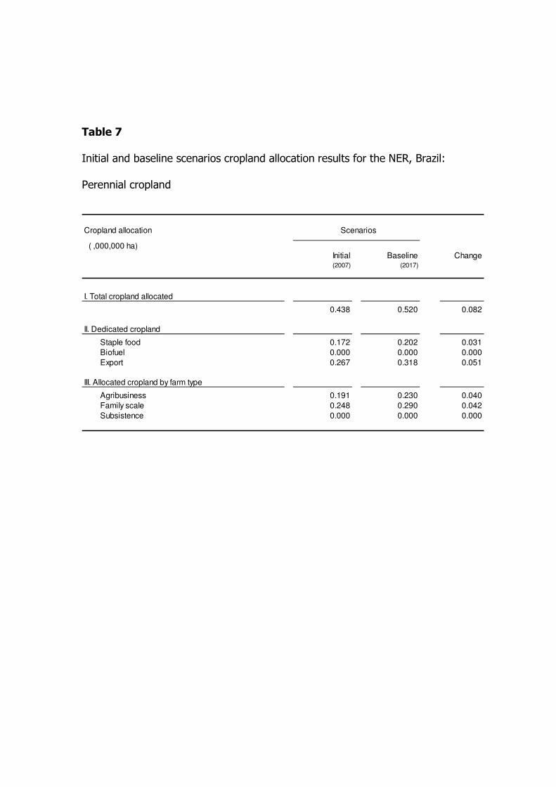
Table 7
Initial and baseline scenarios cropland allocation results for the NER, Brazil:
Perennial cropland
Cropland allocation Scenarios
( ,000,000 ha)Initial Baseline Change(2007) (2017)
I. Total cropland allocated
0.438 0.520 0.082
II. Dedicated cropland
Staple food 0.172 0.202 0.031
Biofuel 0.000 0.000 0.000
Export 0.267 0.318 0.051
III. Allocated cropland by farm type
Agribusiness 0.191 0.230 0.040
Family scale 0.248 0.290 0.042
Subsistence 0.000 0.000 0.000

Table 8
Cropland allocation impacts for the NER, Brazil: Initial (2007) and baseline
(2017) scenarios
Indicator / objective Scenarios
Initial Baseline Change(2007) (2017)
I. Regional biofuel production (% of regional demand)
Ethanol 100% 82% -18%
Biodiesel 0% 0% -
II. Economic indicators ( ,000,000 R$)
1. Staple food feedstock -5,476 -6,313 -15%
2. Agriculture commodity export 2,873 6,429 124%
3. Biofuel feedstock 407 648 59%
4. Fuel balance -3,115 -5,890 -89%
III. Regional development objectives
1. Staple food feedstock autonomy (%) 64% 66% 4%
2. Fuel feedstock autonomy (%) 55% 38% -31%
3. Comprehensive feedstock economic impact ( M R$) -5,312 -5,126 3%
4. Job positions @ farm level ( ,000 jobs) 1,153 1,257 9%

Table 9
Individual optimal results for the four objectives in the 2017 cropland allocation
model, NER, Brazil (payoff matrix)*
Objective Unit Baseline Max.
Staple food Energy Comprehen. Jobs
autonomy autonomy balance
Staple food autonomy (%) 66% 77% 24% 59% 27%
Energy (fuel) autonomy (%) 38% 29% 81% 71% 70%
Comprehensive trade balance ( ,000,000 R$) (5,126) (2,250) (4,351) 59 (217)
Job positions at farm level ( ,000 jobs) 1,257 1,518 1,528 1,533 1,538
* diagonal elements in bold in the dotted area reflect ideal solutions for each of the objectives in the model

Table 10
Baseline and CP optimized scenarios cropland allocation results for the NER,
Brazil: (2017): Annual cropland
Cropland Baseline CP optimized scenarios
( ,000,000 ha) B5 B5+ec B5+m B10+m
I. Total cropland allocated
12.807 14.575 14.575 14.575 14.575
II. Dedicated cropland
Staple food 8.002 9.386 9.400 9.406 9.411Export 4.154 1.035 1.641 1.702 1.761Biofuel 0.651 4.154 3.534 3.467 3.404
III. Allocated cropland by farm type
Agribusiness 6.751 7.209 7.209 7.209 7.209Family scale 5.694 6.935 6.935 6.935 6.935Subsistence 0.362 0.432 0.432 0.432 0.432
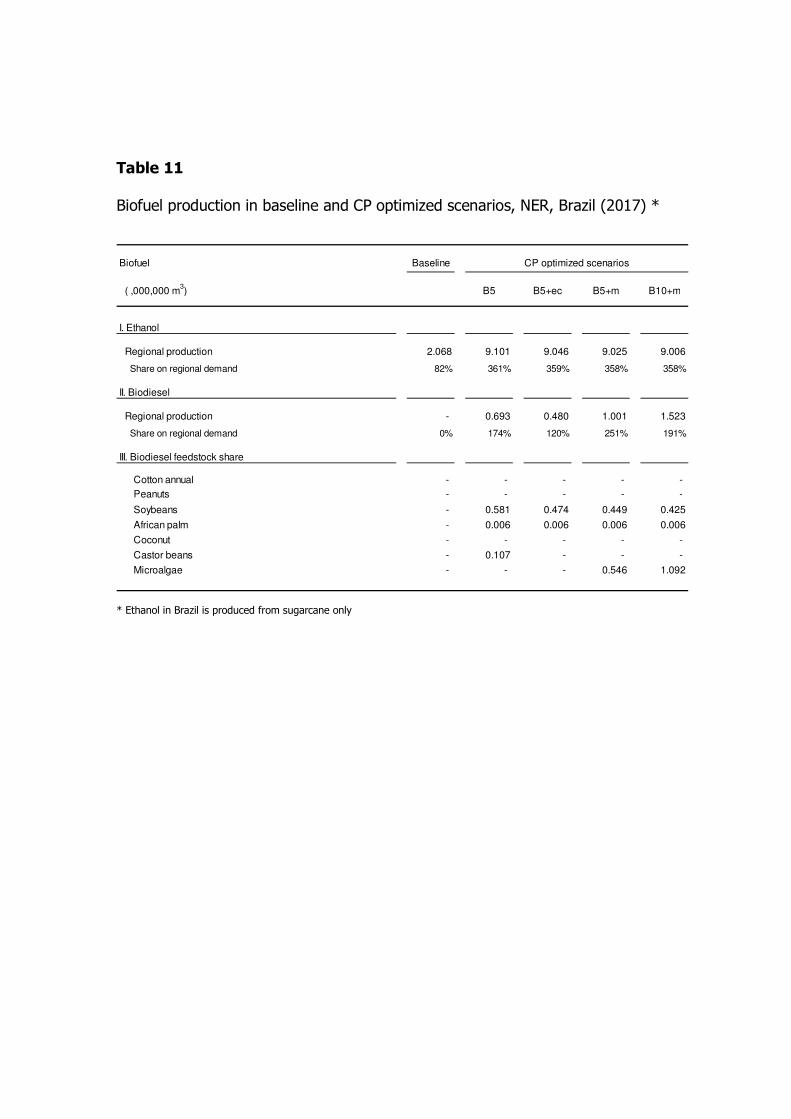
Table 11
Biofuel production in baseline and CP optimized scenarios, NER, Brazil (2017) *
Biofuel Baseline CP optimized scenarios
( ,000,000 m3) B5 B5+ec B5+m B10+m
I. Ethanol
Regional production 2.068 9.101 9.046 9.025 9.006
Share on regional demand 82% 361% 359% 358% 358%
II. Biodiesel
Regional production - 0.693 0.480 1.001 1.523
Share on regional demand 0% 174% 120% 251% 191%
III. Biodiesel feedstock share
Cotton annual - - - - -
Peanuts - - - - -
Soybeans - 0.581 0.474 0.449 0.425
African palm - 0.006 0.006 0.006 0.006
Coconut - - - - -
Castor beans - 0.107 - - -
Microalgae - - - 0.546 1.092
* Ethanol in Brazil is produced from sugarcane only

Table 12
Regional feedstock trade balances in baseline and four CP optimized scenarios
for the NER, Brazil (2017)
Economic indicator Baseline CP optimized scenarios
B5 B5+ec B5+m B10+m
Staple food feedstock -6,313 -3,976 -3,948 -3,937 -3,927
Commodity export 6,429 2,499 2,892 2,943 2,991
Biofuel feedstock 648 3,413 3,135 2,226 1,318
Fuel balance -5,890 -2,471 -2,629 -2,308 -1,987

Table 13
Baseline and CP multiple objective optimization results for four model objectives
applied to the NER, Brazil (2017)
Model objectives Baseline CP optimized scenarios
B5 B5+ec B5+m B10+m
Comprehensive feedstock economic impact ( ,000,000 R$) -5,126 -535 -549 -1,077 -1,605
Staple food feedstock autonomy (%) 66% 70% 70% 71% 71%
Fuel feedstock autonomy (%) 38% 74% 72% 76% 79%
Job positions @ farm level ( ,000 jobs) 1,257 1,528 1,528 1,532 1,537

Table 14
Farm land available in the NER (based on 2006 data; published in IBGE, 2009)
Region Land use availability ( ,000,000 ha)
Permanent Annual Rangeland Forest
crops crops /pasture /timber
Northeast (NE) 5.237 16.978 32.649 25.579
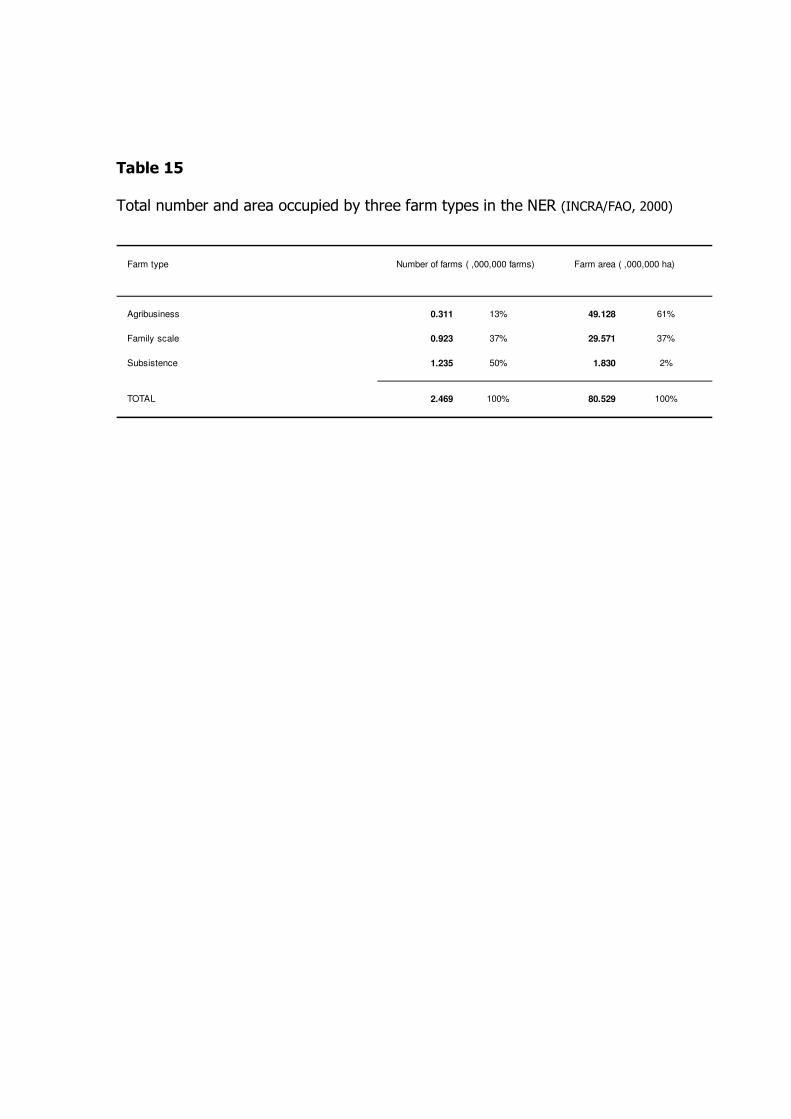
Table 15
Total number and area occupied by three farm types in the NER (INCRA/FAO, 2000)
Farm type Number of farms ( ,000,000 farms) Farm area ( ,000,000 ha)
Agribusiness 0.311 13% 49.128 61%
Family scale 0.923 37% 29.571 37%
Subsistence 1.235 50% 1.830 2%
TOTAL 2.469 100% 80.529 100%

Figure 1 Simplified diagram showing the relations between available cropland,
cropland use, farm type and feedstock destinations as followed in this study
Available cropland
Annual
Perennial
Agribusiness farms
Family scale farms
Subsistence farms
Commodity export
Staple food
Biofuel

-
1.00
2.00
3.00
4.00
5.00
6.00
-
2.00
4.00
6.00
8.00
10.00
12.00
Pere
nnia
l cro
pla
nd
( ,
000,0
00 h
a)
Annual cro
pla
nd
( ,
000,0
00 h
a)
Annual
Permanent
Figure 2 Historical annual and perennial cropland evolution in the NER,
Brazil (IBGE, 2009)

-
20,000
40,000
60,000
80,000
1999 2000 2001 2002 2003 2004 2005 2006 2007 2008
,00
0 b
oe
Land
Ocean
Total
Figure 3 Petroleum extraction evolution in the NER, Brazil (ANP, 2009)

0%
10%
20%
30%
40%
50%
60%
70%
80%
90%
100%
Baseline CP optimized scenarios
Beans
Cassava
Corn
Rice
Sugarcane
Figure 4 Average regional staple food autonomy results for selected crops in
baseline and four CP scenarios, NER, Brazil (2017)

-1.500
-1.000
-0.500
0.000
0.500
1.000
1.500
2.000
Baseline CP scenarios Difference
I. Sugarcane
Staple food
Biofuel
Export
-1.000
-0.500
0.000
0.500
1.000
1.500
2.000
Baseline CP scenarios Difference
II. Soybeans
Staple food
Biofuel
Export
Figure 5 Average cropland allocation shifts between the baseline and CP
optimized scenarios for the NER, Brazil (2017): I. Sugarcane; II. Soybeans

0.000
0.200
0.400
0.600
0.800
1.000
1.200
B5 B5+ec B5+m B10+m
CP scenarios
Soybeans
African palm
Castor beans
Microalgae
Figure 6 Biodiesel feedstock sources cropland allocations in four CP scenarios
for the NER, Brazil (2017)

16%
4% 2% 1%
0%
10%
20%
30%
40%
50%
60%
70%
80%
90%
100%
B5 B5+ec B5+m B10+m
CP scenarios
Agribusiness
type
Family scale
type
Figure 7 Farm type participation in biodiesel feedstock production in four CP
scenarios outlined for the NER, Brazil (2017)