BIOINF525: INTRODUCTION TO BIOINFORMATICS LAB SESSION 3

Protein Structure Visualization and Small Molecule Dockinghttp://bioboot.github.io/bioinf525_w17/module1/#1.3

Dr. Barry GrantJan 2017

Section 1: Introduction to the RCSB Protein Data Bank (PDB)The PDB archive is the major repository of information about the 3D structures of large biological molecules, including proteins and nucleic acids. Understanding the shape of these molecules helps to understand how they work. This knowledge can be used to help deduce a structure's role in human health and disease, and in drug development. The structures in the PDB range from tiny proteins and bits of DNA or RNA to complex molecular machines like the ribosome composed of many chains of protein and RNA.

In the first section of this lab we will interact with the main US based PDB website (note there are also sites in Europe and Japan).

Visit: http://www.rcsb.org/ and answer the following questions

NOTE: The “Analyze” -> “PDB Statistics” on the PDB home page should allow you to determine most of these answers.

Q1: What proportion of PDB entries does X-ray crystallography account for? What proportion of structures are protein?

Q2: Type HIV in the search box on the home page and determine how many HIV-1 protease structures are in the current PDB?

Now download the “PDB File” for the HIV-1 protease structure with the PDB identifier 1HSG. On the website you can “Display” the contents of this “PDF format” file. Alternatively, you can examine the contents of your downloaded file in a suitable text editor.

NOTE: On Windows you can use NotePad whilst on Mac you can try using the Terminal application. For the later open Terminal and try the following command:

> more ~/Downloads/1hsg.pdb ## (use ‘q’ to quit)

NOTE: You can type 1HSG in the PDB search box to jump to its entry and then click “Download Files” to the right of the top display. Selecting “Display Files” will allow you to view the PDB file directly in your browser window.

When viewing the file stop when you come the lines beginning with the word “ATOM”. We will discuss this ubiquitous PDB file format when you have got this far.

! 1

Section 2: Visualizing the HIV-1 protease structureThe HIV-1 protease [1] is an enzyme that is vital for the replication of HIV. It cleaves newly formed polypeptide chains at appropriate locations so that they form functional proteins. Hence, drugs that target this protein could be vital for suppressing viral replication. A handful of drugs - called HIV-1 protease inhibitors (saquinavir, ritonavir, indinavir, nelfinavir, etc.) [2] - are currently commercially available that inhibit the function of this protein, by binding in the catalytic site that typically binds the polypeptide.

Figure 1. HIV-1 protease structure in complex with the small molecule indinavir.

In this section we will use the 2Å resolution X-ray crystal structure of HIV-1 protease with a bound drug molecule indinavir (PDB ID: 1HSG) [3]. We will use the VMD molecular viewer to visually inspect the protein, the binding site and the drug molecule. After exploring features of the complex we will move on to computationally dock a couple of drug molecules into the binding site of HIV-1 protease to see how well computational docking can reproduce the crystallographically observed binding pose. If time permits, we will also explore the conformational dynamics and flexibility of the protein - important for it’s function and for considering during drug design.

Open VMD and load 1hsg.pdb by using the VMD Main window and going to "File" -> "New Molecule” and then from the new window that appears click “Browse” and select your downloaded 1hsg.pdb file. Then click “Load”.

You should now see the protein structure displayed as lines and water molecules as little red dots. Use the mouse to zoom and rotate. Once you have the hang of rotation we will start exploring different “Graphical Representations”.

VMD can display molecules in various ways by choosing different options in the Graphical Representations window shown in Figure 2. You can access this window by clicking Graphics > Representations from the small VMD Main window.

! 2

NOTE. Each representation is defined by three main parameters: (1) the drawing method, (2) the selected atoms to be included in the representation, and (3) the coloring method (see Figure 2 labels 1-3)

Figure 2. The VMD graphical Representation window. Note that (1) the drawing method defines which graphical representation is used and (2) the selection determines which part of the molecule is drawn, and (3) defines the color it is displayed with. You are encouraged to explore different drawing styles (Drawing Methods - labeled 1) including Licorice, Tube and NewCartoon (see below for examples A-C).

Also try different selections by entering text in the (Selected Atoms box - labeled 2). Some examples to try include: chain A and backbone resname ASP within 5 of resname MK1

Using Atom SelectionsNow type “protein” in the Selected Atoms text box (labeled 2 in Figure 2) and show the protein using the Cartoon representation and color by chain (see label 3 in Figure 2.)

Lets add a new representation by clicking the “Create Rep” (circled in Figure 2) and using the selection text “not protein and not water”

Add more representations (by clicking the “Create Rep” button) and hiding (by double clicking) or deleting previous ones (with the “Delete Rep” button) to explore different representations for both the ligand and the protein.

NOTE: you can use the residue name of the ligand “resname MK1” to select just the ligand.

Water molecules have the residue name HOH. Select and display all water molecules as red spheres. If you think the spheres are too big, how would you reduce their size?

! 3

3

Q3: Water molecules normally have 3 atoms. Why do we see just one atom per water molecule in this structure?

Q4: There is a conserved water molecule in the binding site. Can you identify this water molecule? What residue number does this water molecule have (see note below)?

NOTE: From the VMD Main window click Mouse > Label > Atoms and then click on the water in question to display its residue number. A short cut is to press the #1 key when your mouse is active in the OpenGL window.

Now you should be able to produce an image similar or even superior to Figure 1 and save it to an image file on disk with VMD Main window, File > Render > Start Rendering.

NOTE: You can chose different rendering engines including Tachyon (internal), which is commonly used for publication quality images.

Optional: Generate and save a figure clearly showing the two distinct chains of HIV-protease along with the ligand. You might also consider showing the catalytic residues ASP 25 in each chain (we recommend Licorice for these side-chains). Email this figure to bjgrant@umich.edu for grading.

Discussion Topic: Can you think of a way in which indinavir, or even larger ligands and substrates, could enter the binding site?

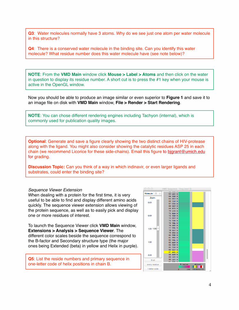
Sequence Viewer ExtensionWhen dealing with a protein for the first time, it is very useful to be able to find and display different amino acids quickly. The sequence viewer extension allows viewing of the protein sequence, as well as to easily pick and display one or more residues of interest.

To launch the Sequence Viewer click VMD Main window, Extensions > Analysis > Sequence Viewer. The different color scales beside the sequence correspond to the B-factor and Secondary structure type (the major ones being Extended (beta) in yellow and Helix in purple).

Q5: List the reside numbers and primary sequence in one-letter code of helix positions in chain B.

! 4

Q6: As you have hopefully observed HIV protease is a homodimer (i.e. it is composed of two identical chains). With the aid of the graphic display and the sequence viewer extension can you identify secondary structure elements that are likely to only form in the dimer rather than the monomer?

Section 3: In silico docking of drugs to HIV-1 protease Docking algorithms require each atom to have a charge and an atom type that describes its properties. However, typical PDB structures don’t contain this information. We therefore have to ‘prep’ the protein and ligand files to include these values along with their atomic coordinates. All this will be done in a tool called AutoDock Tools (adt).

3.1 Prepare the proteinThe PDB file (1hsg.pdb) contains protein, ligand and water oxygen atoms. First we have to extract just the protein atoms, which are the lines that start with the keyword ATOM. Each protein chain is terminated with a line that starts with TER. (If you would like to confirm this, open 1hsg.pdb in a text editor and scroll through the text.) You could copy and paste the protein portion of the original PDB file into a new file. Here we will use VMD to save a new protein only PDB format file.

To keep your work organized, first create a new folder or directory on your Desktop called lab3.

Then from the VMD Main window make sure your 1hsg molecule is selected by clicking on it. Then select File > Save Coordinates... Type "protein" under selected atoms and save a new PDB file to your lab3 folder called “1hsg_protein.pdb".

Launch AutoDock Tools (ADT) from the Desktop icon on Windows or using the Finder on Mac (from Applications > MGLTools > AutoDocTools ).

NOTE: First time opening of ADT can be a rather slow process as it completes some initial configuration. Be patient and resist the urge to click many times and thus open multiple instances.

In ADT load the protein using File > Read Molecule. Select 1hsg_protein.pdb. Click Open.

Note: In ADT, you can translate the molecule by clicking and holding down the right mouse button while moving the mouse, rotate by clicking and holding down the middle button and zoom in/out by using the scroll wheel of the mouse.

Bonds and atoms are shown in white. For better visualization, color the structure by atom type - Color > By Atom Type. Click All Geometries and then OK.

! 5

Q7: Can you locate the binding site visually? Note that crystal structures normally lack hydrogen atoms, why?

As we have already noted (remind me if we haven’t) crystal structures normally lack hydrogen atoms. However, hydrogen atoms are required for appropriate treatment of electrostatics during docking so we need to add hydrogen atoms to the structure using Edit > Hydrogen > Add. Click OK. You should see a lot of white dashes where the hydrogens were added.

Now we need to get ADT to assign charges and atom type to each atom in the protein. We do this with Grid > Macromolecule > Choose.... Choose 1hsg_protein in the popup window and click Select Molecule.

ADT will merge non-polar hydrogens, assign charges and prompt you to save the macromolecule.

Save this molecule to your lab3 folder with the default file extension of “pdbqt” (i.e. a new file called 1hsg_protein.pdbqt). Open this in a text editor and look at the last two columns - these should be the charge and atom type for each atom.

Q8: Look at the charges. Does it make sense (e.g. based on your knowledge of the physiochemical properties of amino acids)?

Now, we need to define the 3D search space were ligand docking will be attempted. Remember the binding site that you observed in one of the earlier steps. Ideally, if we do not know the binding site, we will either define a box that encloses the whole protein or perhaps a specific region of the protein. In this case, to speed up the docking process, we will define a search space that encloses the known binding site.

To define the box, use Grid > Grid Box.... This will draw a box with opposite faces colored in red, green and blue. Fiddle with the dials and see how you can enclose regions of the protein. In this instance we will use a Spacing (angstrom) of 1Å (this is essentially a scaling factor). So set this dial to 1.000. So that we all get consistent results, let us set the (x, y, z) center as (16, 25, 4) and the number of points in (x, y, z)-dimension as (30, 30, 30). Make a note of these values. We will need it later.

Close the Grid Options dialog by clicking File > Close w/out saving.

That is all we need to do with the protein file. Delete it from the display using Edit > Delete > Delete Molecule and select 1HSG_protein. Click Delete Molecule and CONTINUE.

! 6

3.2 Prepare the ligandLike the protein, the ligand lacks hydrogen atoms. We need to add hydrogen atoms and also optionally define rotatable bonds that can be used for ‘flexible docking’. You can run through this yourself using the instructions in Appendix 1. However, to expedite your progress we have already done this for you. You can download the file from:

http://bioboot.github.io/bioinf525_w17/class-material/indinavir.pdbqt

Move this file to your lab3 folder.

3.3 Prepare a docking configuration fileBefore we can perform the actual docking, we need to create an input file that defines the protein, ligand and the search parameters. We will create the input file in a text editor.If you have used Unix/Linux before, open your favorite text editor (e.g. vi, emacs, nano) or use a GUI based editor such as gedit. Windows users can use NotePad.

The input file should look something like:

receptor = 1hsg_protein.pdbqtligand = indinavir.pdbqt

num_modes = 50

out = all.pdbqt

center_x = XXcenter_y = XXcenter_z = XX

size_x = XXsize_y = XXsize_z = XX

seed = 2009

This defines your protein (receptor), ligand (ligand) number of docking modes to generate (num_modes). All the docked modes will be collated in a file defined by out (all.pdbqt). You should replace the XX with the center of your 3D search space (center_x/y/z) and the size of the box (size_x/y/z) that you defined in Section 3.1 “Prepare the protein" above.

Save the file as config.txt in your lab3 folder.

Again if necessary you can download a pre-prepared file from here: http://bioboot.github.io/bioinf525_w17/class-material/config.txt

! 7

3.4 Docking indinavir into HIV-1 protease For this portion of the practical, we will use a program called Autodock Vina [4]. Autodock Vina is a fast docking program that requires minimal user intervention and is often employed for high-throughput virtual screening. We will run it from a terminal.

Make sure you are in your lab3 folder containing the three files 1hsg_protein.pdbqt, indinavir.pdbqt and config.txt files.

On Mac you can use the Unix commands below to change directory and list files respectively:

> cd ~/Desktop/lab3 > ls

On Windows you can use these equivalent commands:

> CD Desktop/lab3 > dir

Now we are ready to run vina to perform the docking. We will keep a log of all program output in a file log.txt

Again the commands to run the program are different on Mac and Windows. For Mac use:

> ~/Downloads/autodock_vina_1_1_2_mac/bin/vina --config config.txt --log log.txt

On Windows use:

> "\Program Files\The Scripps Research Institute\Vina\vina.exe" --config config.txt --log log.txt

NOTE: This will take a few minutes depending on how fast your computer is. While you wait, if you are interested, read [1] for a review on HIV-1 protease structure, function and drug discovery.

Once the run is complete, you should have two new files all.pdbqt, which contains all the docked modes, and log.txt, which contains a table of calculated affinities based on AutoDock Vina's scoring function [4]. The best docked mode, according to AutoDock Vina, is the first entry in all.pdbqt.

! 8

In order to visualize the docks and compare to the crystal conformation of the ligand we will process the all.pdbqt to a PDB format file that can be loaded into VMD. To do this we will use the following commands:

On Mac:

> egrep "^(MODEL|ENDMDL|HETATM)" all.pdbqt > results.pdb

On Windows:

> FINDSTR /c:"MODEL" /c:"ENDMDL" /c:"HETATM" all.pdbqt > results.pdb

NOTE: If these commands don't work for you then you can manually remove all lines in the all.pdbqt file that do not begin with the words MODEL, ENDMDL or HETATM.

Now load both the original 1hsg.pdb file and your new results.pdb file into VMD. You will need to use VMD Main > File > New Molecule for each file.

Begin by displaying the protein in cartoon representation, indinavir in licorice (also called stick representation) and the docked conformations as licorice as well.

Cycle through the docks by clicking the playback control buttons on the lower right hand corner of the VMD Main window.

Q9: Qualitatively, how good are the docks? Is the crystal binding mode reproduced? Is it the best conformation according to AutoDock Vina?

NOTE: To assess the results quantitatively we could calculate the RMSD (root mean square distance) between each of the docking results and the known crystal structure (see for example Extensions > Analysis > RMSD Calculator). However, for most applications we wont know the answer a priori so the calculated binding affinity (see your log.txt file for details), scoring function and additional docking energy assessments become all-important.

Q10: What one part of this lab or associated lecture material is still confusing? If appropriate please also indicate the question number from this lab instruction pdf and answer the question in the following anonymous form: http://tinyurl.com/bioinf525-lab1-3

! 9

(Optional) Section 4: Exploring the conformational dynamics of proteinsVisit the new web application Bio3D-web: http://thegrantlab.org/bio3d/webapps watch the introduction video and and click start analysis to begin exploring the conformational dynamics and flexibility of protein structures.

Concluding remarksIn this practical, we have looked at how small molecules could be docked into a protein. This approach is widely used to detect binding sites and also to screen a library of small molecules to find potential drugs that could bind to a known binding site. Scoring functions play an important role in identifying a "good dock" and as such remains an area of active research. Several other considerations are worth noting including water molecules and ions in the binding site, flexibility of binding site residues, etc. Some docking programs (including AutoDock Vina) allow you to define a subset of flexible sidechains. Whilst this permits binding site rearrangement to accommodate distinct ligands, the computational search space increases many fold. Defining water molecules that are important in the binding site also remains an area of active research. In this practical, we have considered only protein-ligand docking. Protein-protein docking is also widely used, but not considered here due to the significantly higher search space that has to be considered. As the number of solved protein structures continues to grow, in silico docking will play an increasingly important role in the drug discovery process.

References:1. Brik A, Wong CH. "HIV-1 protease: mechanism and drug discovery". Org. Biomol. Chem.

(2003) 1:5–14. http://pubs.rsc.org/en/Content/ArticleLanding/2003/OB/b208248a

2. Wensing AM, van Maarseveen NM, Nijhuis M. "Fifteen years of HIV Protease Inhibitors: raising the barrier to resistance." Antiviral Res. (2009).http://www.sciencedirect.com/science/article/pii/S0166354209004902

3. Chen Z, Li Y, Chen E, Hall DL, Darke PL, Culberson C, Shafer JA, Kuo LC. "Crystal structure at 1.9-A resolution of human immunodeficiency virus (HIV) II protease complexed with L-735,524, an orally bioavailable inhibitor of the HIV proteases." J. Biol. Chem. (1994) 269:26344-26348.http://www.jbc.org/content/269/42/26344.long

4. Trott O, Olson AJ. "AutoDock Vina: improving the speed and accuracy of docking with a new scoring function, efficient optimization and multithreading", J. Comput. Chem. (2009).http://onlinelibrary.wiley.com/doi/10.1002/jcc.21334/abstract

5. Baker NA, Sept D, Joseph S, Holst MJ, McCammon JA. "Electrostatics of nanosystems: application to microtubules and the ribosome." Proc. Natl. Acad. Sci. (2001) 98:10037-10041.http://www.pnas.org/content/98/18/10037

! 10

Appendix I:

First, extract the ligand atoms from the PDB 1hsg.pdb. As mentioned in Exercise 2, the ligand residue name for indinavir in the PDB file is MK1 and the lines start with the keyword HETATM for heteroatoms. In a terminal type:

> grep "^HETATM.*MK1" 1hsg.pdb > indinavir.pdb

Load the ligand structure into ADT using File > Read Molecule and select indinavir.pdb

Again, color by atom type. Color > By Atom Type. Click All Geometries and then OK.

Now we have to add polar hydrogen atoms. Add all hydrogen atoms initially. Non polar hydrogens will be merged in the next step. Edit > Hydrogens > Add. Select All Hydrogens and click OK.

Define this as the ligand in ADT so that ADT assigns partial charges and sets rotatable ligand bonds using Ligand > Input > Choose.... Select indinavir and click Select Molecule for AutoDock4. You should see a message that confirms that non-polar hydrogens have been merged, charges added and rotatable bond detected. Click OK. The ligand will now have only polar hydrogens.

To check the rotatable bonds detected by ADT, go to Ligand > Torsion Tree > Choose Torsions.... You should see 14 rotatable bonds.

Click Done and save the ligand file in PDBQT format. Do this using Ligand > Output > Save as PDBQT.... Click Save to save the file as indinavir.pdbqt.Quit ADT using File > Exit > OK.

Appendix II: Useful resources/links

This document and all associated input and output files are available online at http://thegrantlab.org/teaching/ under “BIOINF525/524 (Module 1, Lab 1.3, Structural Bioinformatics)”. All required software is freely available from the sites listed below.

VMD http://www.ks.uiuc.edu/Research/vmd/AutoDock Tools http://mgltools.scripps.edu/downloadsAutoDock Vina http://vina.scripps.edu/download.html

NOTE: For installing AutoDock Tools on newer mac OS versions you will need to “control-click” (i.e. hold down the control key as you click your mouse on the downloaded .dmg file) to open the disc image and then select Open to begin the install.

! 11

Appendix III: Basic Unix commands

ls # list files in current directory.cd dir # change directory to the directory 'dir'pwd # print the current working directory on the screenrm file # delete (remove) 'file'mv file newfile # rename file to newfilecat file # print the contents of file to the screenmore file # print file to the screen with more navigationmkdir dirname # make a new directory/folder

Windows equivalents

dir # list files in current directoryCD dir # change directory to the directory 'dir'cd # print the current working directory on the screendel file # delete (remove) 'file'MD dirname # make a new directory/folder

! 12