biologically inspired dynamic textures for probing...
TRANSCRIPT
Biologically Inspired Dynamic Texturesfor Probing Motion Perception
Jonathan VacherCNRS UNIC and Ceremade
Univ. Paris-Dauphine75775 Paris Cedex 16, FRANCE
Andrew Isaac MesoInstitut de Neurosciences de la Timone
UMR 7289 CNRS/Aix-Marseille Universite13385 Marseille Cedex 05, [email protected]
Laurent PerrinetInstitut de Neurosciences de la Timone
UMR 7289 CNRS/Aix-Marseille Universite13385 Marseille Cedex 05, FRANCE
Gabriel PeyreCNRS and CeremadeUniv. Paris-Dauphine
75775 Paris Cedex 16, [email protected]
Abstract
Perception is often described as a predictive process based on an optimal inferencewith respect to a generative model. We study here the principled constructionof a generative model specifically crafted to probe motion perception. In thatcontext, we first provide an axiomatic, biologically-driven derivation of the model.This model synthesizes random dynamic textures which are defined by stationaryGaussian distributions obtained by the random aggregation of warped patterns.Importantly, we show that this model can equivalently be described as a stochasticpartial differential equation. Using this characterization of motion in images, itallows us to recast motion-energy models into a principled Bayesian inferenceframework. Finally, we apply these textures in order to psychophysically probespeed perception in humans. In this framework, while the likelihood is derivedfrom the generative model, the prior is estimated from the observed results andaccounts for the perceptual bias in a principled fashion.
1 Motivation
A normative explanation for the function of perception is to infer relevant hidden parameters fromthe sensory input with respect to a generative model [7]. Equipped with some prior knowledgeabout this representation, this corresponds to the Bayesian brain hypothesis, as has been perfectlyillustrated by the particular case of motion perception [19]. However, the Gaussian hypothesisrelated to the parameterization of knowledge in these models —for instance in the formalizationof the prior and of the likelihood functions— does not always fit with psychophysical results [17].As such, a major challenge is to refine the definition of generative models so that they conform tothe widest variety of results.
From this observation, the estimation problem inherent to perception is linked to the definition of anadequate generative model. In particular, the simplest generative model to describe visual motionis the luminance conservation equation. It states that luminance I(x, t) for (x, t) ∈ R2 × R isapproximately conserved along trajectories defined as integral lines of a vector field v(x, t) ∈ R2 ×R. The corresponding generative model defines random fields as solutions to the stochastic partialdifferential equation (sPDE),
〈v, ∇I〉+∂I
∂t= W, (1)
1
where 〈·, ·〉 denotes the Euclidean scalar product in R2, ∇I is the spatial gradient of I . To matchthe statistics of natural scenes or some category of textures, the driving term W is usually definedas a colored noise corresponding to some average spatio-temporal coupling, and is parameterizedby a covariance matrix Σ, while the field is usually a constant vector v(x, t) = v0 accounting for afull-field translation with constant speed.
Ultimately, the application of this generative model is essential for probing the visual system, forinstance to understand how observers might detect motion in a scene. Indeed, as shown by [9, 19],the negative log-likelihood corresponding to the luminance conservation model (1) and deter-mined by a hypothesized speed v0 is proportional to the value of the motion-energy model [1]||〈v0, ∇(K ? I)〉 + ∂(K?I)
∂t ||2, where K is the whitening filter corresponding to the inverse of Σ,and ? is the convolution operator. Using some prior knowledge on the distribution of motions, forinstance a preference for slow speeds, this indeed leads to a Bayesian formalization of this inferenceproblem [18]. This has been successful in accounting for a large class of psychophysical observa-tions [19]. As a consequence, such probabilistic frameworks allow one to connect different modelsfrom computer vision to neuroscience with a unified, principled approach.
However the model defined in (1) is obviously quite simplistic with respect to the complexity of natu-ral scenes. It is therefore useful here to relate this problem to solutions proposed by texture synthesismethods in the computer vision community. Indeed, the literature on the subject of static texturessynthesis is abundant (see [16] and the references therein for applications in computer graphics).Of particular interest for us is the work of Galerne et al. [6], which proposes a stationary Gaussianmodel restricted to static textures. Realistic dynamic texture models are however less studied, andthe most prominent method is the non-parametric Gaussian auto-regressive (AR) framework of [3],which has been refined in [20].
Contributions. Here, we seek to engender a better understanding of motion perception by im-proving generative models for dynamic texture synthesis. From that perspective, we motivate thegeneration of optimal stimulation within a stationary Gaussian dynamic texture model. We base ourmodel on a previously defined heuristic [10, 11] coined “Motion Clouds”. Our first contribution is
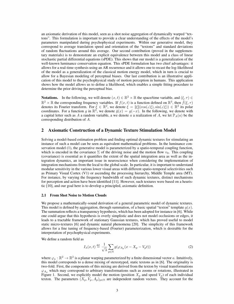
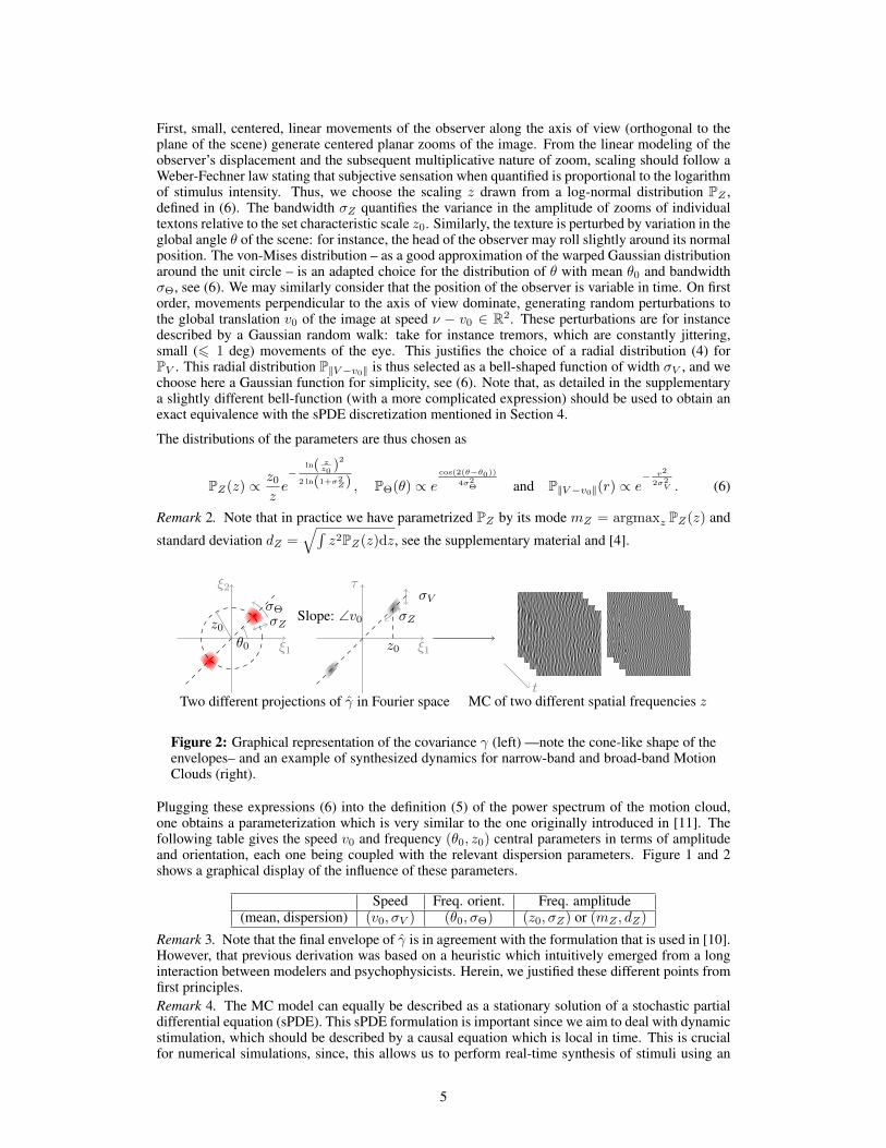
Figure 1: Parameterization of the class of Motion Clouds stimuli. The illustration relates theparametric changes in MC with real world (top row) and observer (second row) movements.(A) Orientation changes resulting in scene rotation are parameterized through θ as shown inthe bottom row where a horizontal a and obliquely oriented b MC are compared. (B) Zoommovements, either from scene looming or observer movements in depth, are characterised byscale changes reflected by a scale or frequency term z shown for a larger or closer object bcompared to more distant a. (C) Translational movements in the scene characterised by Vusing the same formulation for static (a) slow (b) and fast moving MC, with the variability inthese speeds quantified by σV . (ξ and τ) in the third row are the spatial and temporal frequencyscale parameters. The development of this formulation is detailed in the text.
2
an axiomatic derivation of this model, seen as a shot noise aggregation of dynamically warped “tex-tons”. This formulation is important to provide a clear understanding of the effects of the model’sparameters manipulated during psychophysical experiments. Within our generative model, theycorrespond to average translation speed and orientation of the “textons” and standard deviationsof random fluctuations around this average. Our second contribution (proved in the supplemen-tary materials) is to demonstrate an explicit equivalence between this model and a class of linearstochastic partial differential equations (sPDE). This shows that our model is a generalization of thewell-known luminance conservation equation. This sPDE formulation has two chief advantages: itallows for a real-time synthesis using an AR recurrence and it allows one to recast the log-likelihoodof the model as a generalization of the classical motion energy model, which in turn is crucial toallow for a Bayesian modeling of perceptual biases. Our last contribution is an illustrative appli-cation of this model to the psychophysical study of motion perception in humans. This applicationshows how the model allows us to define a likelihood, which enables a simple fitting procedure todetermine the prior driving the perceptual bias.
Notations. In the following, we will denote (x, t) ∈ R2 × R the space/time variable, and (ξ, τ) ∈R2 × R the corresponding frequency variables. If f(x, t) is a function defined on R3, then f(ξ, τ)denotes its Fourier transform. For ξ ∈ R2, we denote ξ = ||ξ||(cos(∠ξ), sin(∠ξ)) ∈ R2 its polarcoordinates. For a function g in R2, we denote g(x) = g(−x). In the following, we denote witha capital letter such as A a random variable, a we denote a a realization of A, we let PA(a) be thecorresponding distribution of A.
2 Axiomatic Construction of a Dynamic Texture Stimulation Model
Solving a model-based estimation problem and finding optimal dynamic textures for stimulating aninstance of such a model can be seen as equivalent mathematical problems. In the luminance con-servation model (1), the generative model is parameterized by a spatio-temporal coupling function,which is encoded in the covariance Σ of the driving noise and the motion flow v0. This coupling(covariance) is essential as it quantifies the extent of the spatial integration area as well as the in-tegration dynamics, an important issue in neuroscience when considering the implementation ofintegration mechanisms from the local to the global scale. In particular, it is important to understandmodular sensitivity in the various lower visual areas with different spatio-temporal selectivities suchas Primary Visual Cortex (V1) or ascending the processing hierarchy, Middle Temple area (MT).For instance, by varying the frequency bandwidth of such dynamic textures, distinct mechanismsfor perception and action have been identified [11]. However, such textures were based on a heuris-tic [10], and our goal here is to develop a principled, axiomatic definition.
2.1 From Shot Noise to Motion Clouds
We propose a mathematically-sound derivation of a general parametric model of dynamic textures.This model is defined by aggregation, through summation, of a basic spatial “texton” template g(x).The summation reflects a transparency hypothesis, which has been adopted for instance in [6]. Whileone could argue that this hypothesis is overly simplistic and does not model occlusions or edges, itleads to a tractable framework of stationary Gaussian textures, which has proved useful to modelstatic micro-textures [6] and dynamic natural phenomena [20]. The simplicity of this frameworkallows for a fine tuning of frequency-based (Fourier) parameterization, which is desirable for theinterpretation of psychophysical experiments.
We define a random field as
Iλ(x, t)def.=
1√λ
∑p∈N
g(ϕAp(x−Xp − Vpt)) (2)
where ϕa : R2 → R2 is a planar warping parameterized by a finite dimensional vector a. Intuitively,this model corresponds to a dense mixing of stereotyped, static textons as in [6]. The originality istwo-fold. First, the components of this mixing are derived from the texton by visual transformationsϕAp which may correspond to arbitrary transformations such as zooms or rotations, illustrated inFigure 1. Second, we explicitly model the motion (position Xp and speed Vp) of each individualtexton. The parameters (Xp, Vp, Ap)p∈N are independent random vectors. They account for the
3
variability in the position of objects or observers and their speed, thus mimicking natural motions inan ambient scene. The set of translations (Xp)p∈N is a 2-D Poisson point process of intensity λ > 0.The following section instantiates this idea and proposes canonical choices for these variabilities.The warping parameters (Ap)p are distributed according to a distribution PA. The speed parameters(Vp)p are distributed according to a distribution PV on R2. The following result shows that themodel (2) converges to a stationary Gaussian field and gives the parameterization of the covariance.Its proof follows from a specialization of [5, Theorem 3.1] to our setting.Proposition 1. Iλ is stationary with bounded second order moments. Its covariance isΣ(x, t, x′, t′) = γ(x− x′, t− t′) where γ satisfies
∀ (x, t) ∈ R3, γ(x, t) =
∫ ∫R2
cg(ϕa(x− νt))PV (ν)PA(a)dνda (3)
where cg = g ? g is the auto-correlation of g. When λ → +∞, it converges (in the sense of finitedimensional distributions) toward a stationary Gaussian field I of zero mean and covariance Σ.
2.2 Definition of “Motion Clouds”
We detail this model here with warpings as rotations and scalings (see Figure 1). These account forthe characteristic orientations and sizes (or spatial scales) in a scene with respect to the observer
∀ a = (θ, z) ∈ [−π, π)× R∗+, ϕa(x)def.= zR−θ(x),
where Rθ is the planar rotation of angle θ. We now give some physical and biological motivationunderlying our particular choice for the distributions of the parameters. We assume that the distribu-tions PZ and PΘ of spatial scales z and orientations θ, respectively (see Figure 1), are independentand have densities, thus considering ∀ a = (θ, z) ∈ [−π, π) × R∗+, PA(a) = PZ(z)PΘ(θ). Thespeed vector ν is assumed to be randomly fluctuating around a central speed v0, so that
∀ ν ∈ R2, PV (ν) = P||V−v0||(||ν − v0||). (4)
In order to obtain “optimal” responses to the stimulation (as advocated by [21]), it makes sense todefine the texton g to be equal to an oriented Gabor acting as an atom, based on the structure ofa standard receptive field of V1. Each would have a scale σ and a central frequency ξ0. Since theorientation and scale of the texton is handled by the (θ, z) parameters, we can impose without loss ofgenerality the normalization ξ0 = (1, 0). In the special case where σ → 0, g is a grating of frequencyξ0, and the image I is a dense mixture of drifting gratings, whose power-spectrum has a closed formexpression detailed in Proposition 2. Its proof can be found in the supplementary materials. We callthis Gaussian field a Motion Cloud (MC), and it is parameterized by the envelopes (PZ ,PΘ,PV ) andhas central frequency and speed (ξ0, v0). Note that it is possible to consider any arbitrary textonsg, which would give rise to more complicated parameterizations for the power spectrum g, but wedecided here to stick to the simple case of gratings.
Proposition 2. When g(x) = ei〈x, ξ0〉, the image I defined in Proposition 1 is a stationary Gaussianfield of covariance having the power-spectrum
∀ (ξ, τ) ∈ R2 × R, γ(ξ, τ) =PZ (||ξ||)||ξ||2 PΘ (∠ξ)L(P||V−v0||)
(−τ + 〈v0, ξ〉
||ξ||
), (5)
where the linear transform L is such that ∀u ∈ R,L(f)(u) =∫ π−π f(−u/ cos(ϕ))dϕ.
Remark 1. Note that the envelope of γ is shaped along a cone in the spatial and temporal domains.This is an important and novel contribution when compared to a Gaussian formulation like a clas-sical Gabor. In particular, the bandwidth is then constant around the speed plane or the orientationline with respect to spatial frequency. Basing the generation of the textures on all possible transla-tions, rotations and zooms, we thus provide a principled approach to show that bandwidth should beproportional to spatial frequency to provide a better model of moving textures.
2.3 Biologically-inspired Parameter Distributions
We now give meaningful specialization for the probability distributions (PZ ,PΘ,P||V−v0||), whichare inspired by some known scaling properties of the visual transformations relevant to dynamicscene perception.
4
First, small, centered, linear movements of the observer along the axis of view (orthogonal to theplane of the scene) generate centered planar zooms of the image. From the linear modeling of theobserver’s displacement and the subsequent multiplicative nature of zoom, scaling should follow aWeber-Fechner law stating that subjective sensation when quantified is proportional to the logarithmof stimulus intensity. Thus, we choose the scaling z drawn from a log-normal distribution PZ ,defined in (6). The bandwidth σZ quantifies the variance in the amplitude of zooms of individualtextons relative to the set characteristic scale z0. Similarly, the texture is perturbed by variation in theglobal angle θ of the scene: for instance, the head of the observer may roll slightly around its normalposition. The von-Mises distribution – as a good approximation of the warped Gaussian distributionaround the unit circle – is an adapted choice for the distribution of θ with mean θ0 and bandwidthσΘ, see (6). We may similarly consider that the position of the observer is variable in time. On firstorder, movements perpendicular to the axis of view dominate, generating random perturbations tothe global translation v0 of the image at speed ν − v0 ∈ R2. These perturbations are for instancedescribed by a Gaussian random walk: take for instance tremors, which are constantly jittering,small (6 1 deg) movements of the eye. This justifies the choice of a radial distribution (4) forPV . This radial distribution P||V−v0|| is thus selected as a bell-shaped function of width σV , and wechoose here a Gaussian function for simplicity, see (6). Note that, as detailed in the supplementarya slightly different bell-function (with a more complicated expression) should be used to obtain anexact equivalence with the sPDE discretization mentioned in Section 4.
The distributions of the parameters are thus chosen as
PZ(z) ∝ z0
ze−
ln( zz0
)2
2 ln(1+σ2Z) , PΘ(θ) ∝ e
cos(2(θ−θ0))
4σ2Θ and P||V−v0||(r) ∝ e
− r2
2σ2V . (6)
Remark 2. Note that in practice we have parametrized PZ by its mode mZ = argmaxz PZ(z) and
standard deviation dZ =√∫
z2PZ(z)dz, see the supplementary material and [4].
z0
σZ
σV
ξ1
τ
Slope: ∠v0
ξ2
ξ1θ0
z0
σΘ
σZ
Two different projections of γ in Fourier spacet
MC of two different spatial frequencies z
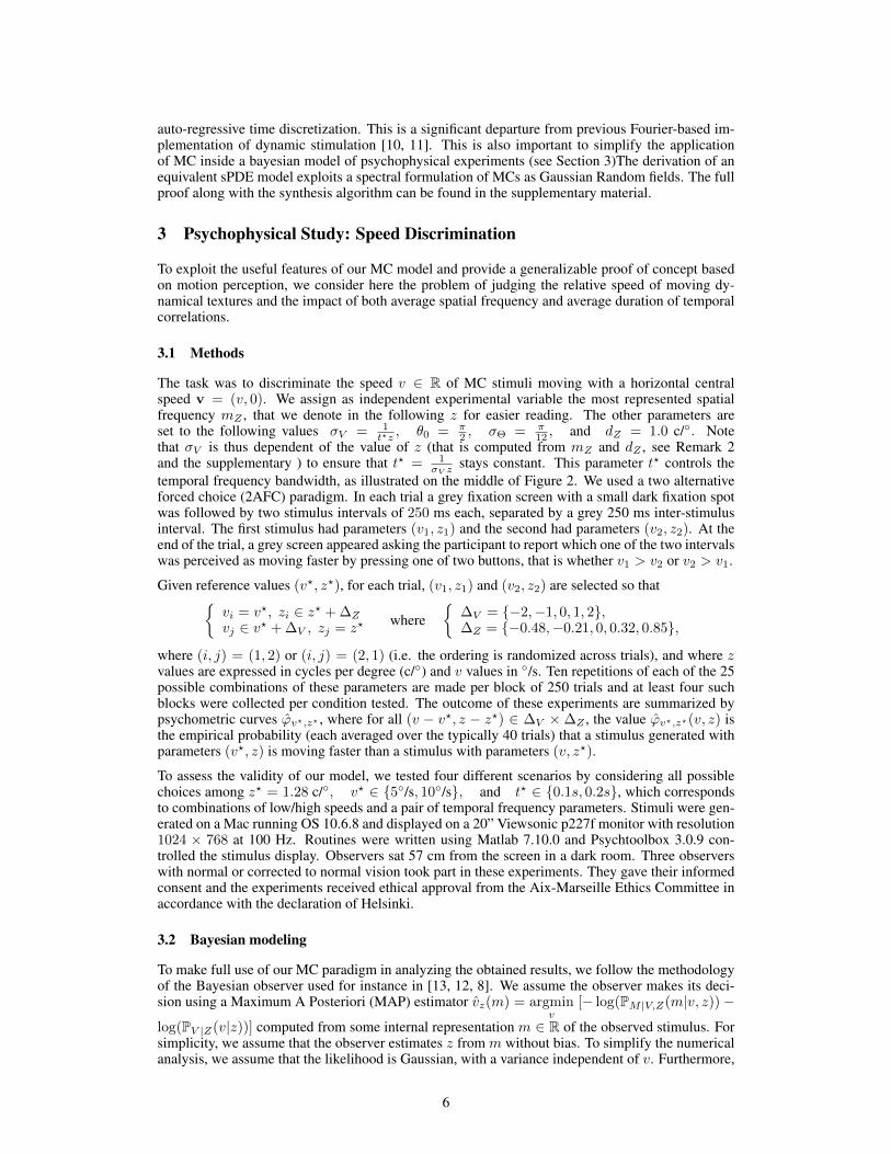
Figure 2: Graphical representation of the covariance γ (left) —note the cone-like shape of theenvelopes– and an example of synthesized dynamics for narrow-band and broad-band MotionClouds (right).
Plugging these expressions (6) into the definition (5) of the power spectrum of the motion cloud,one obtains a parameterization which is very similar to the one originally introduced in [11]. Thefollowing table gives the speed v0 and frequency (θ0, z0) central parameters in terms of amplitudeand orientation, each one being coupled with the relevant dispersion parameters. Figure 1 and 2shows a graphical display of the influence of these parameters.
Speed Freq. orient. Freq. amplitude(mean, dispersion) (v0, σV ) (θ0, σΘ) (z0, σZ) or (mZ , dZ)
Remark 3. Note that the final envelope of γ is in agreement with the formulation that is used in [10].However, that previous derivation was based on a heuristic which intuitively emerged from a longinteraction between modelers and psychophysicists. Herein, we justified these different points fromfirst principles.Remark 4. The MC model can equally be described as a stationary solution of a stochastic partialdifferential equation (sPDE). This sPDE formulation is important since we aim to deal with dynamicstimulation, which should be described by a causal equation which is local in time. This is crucialfor numerical simulations, since, this allows us to perform real-time synthesis of stimuli using an
5
auto-regressive time discretization. This is a significant departure from previous Fourier-based im-plementation of dynamic stimulation [10, 11]. This is also important to simplify the applicationof MC inside a bayesian model of psychophysical experiments (see Section 3)The derivation of anequivalent sPDE model exploits a spectral formulation of MCs as Gaussian Random fields. The fullproof along with the synthesis algorithm can be found in the supplementary material.
3 Psychophysical Study: Speed Discrimination
To exploit the useful features of our MC model and provide a generalizable proof of concept basedon motion perception, we consider here the problem of judging the relative speed of moving dy-namical textures and the impact of both average spatial frequency and average duration of temporalcorrelations.
3.1 Methods
The task was to discriminate the speed v ∈ R of MC stimuli moving with a horizontal centralspeed v = (v, 0). We assign as independent experimental variable the most represented spatialfrequency mZ , that we denote in the following z for easier reading. The other parameters areset to the following values σV = 1
t?z , θ0 = π2 , σΘ = π
12 , and dZ = 1.0 c/◦. Notethat σV is thus dependent of the value of z (that is computed from mZ and dZ , see Remark 2and the supplementary ) to ensure that t? = 1
σV zstays constant. This parameter t? controls the
temporal frequency bandwidth, as illustrated on the middle of Figure 2. We used a two alternativeforced choice (2AFC) paradigm. In each trial a grey fixation screen with a small dark fixation spotwas followed by two stimulus intervals of 250 ms each, separated by a grey 250 ms inter-stimulusinterval. The first stimulus had parameters (v1, z1) and the second had parameters (v2, z2). At theend of the trial, a grey screen appeared asking the participant to report which one of the two intervalswas perceived as moving faster by pressing one of two buttons, that is whether v1 > v2 or v2 > v1.
Given reference values (v?, z?), for each trial, (v1, z1) and (v2, z2) are selected so that{vi = v?, zi ∈ z? + ∆Z
vj ∈ v? + ∆V , zj = z?where
{∆V = {−2,−1, 0, 1, 2},∆Z = {−0.48,−0.21, 0, 0.32, 0.85},
where (i, j) = (1, 2) or (i, j) = (2, 1) (i.e. the ordering is randomized across trials), and where zvalues are expressed in cycles per degree (c/◦) and v values in ◦/s. Ten repetitions of each of the 25possible combinations of these parameters are made per block of 250 trials and at least four suchblocks were collected per condition tested. The outcome of these experiments are summarized bypsychometric curves ϕv?,z? , where for all (v − v?, z − z?) ∈ ∆V ×∆Z , the value ϕv?,z?(v, z) isthe empirical probability (each averaged over the typically 40 trials) that a stimulus generated withparameters (v?, z) is moving faster than a stimulus with parameters (v, z?).
To assess the validity of our model, we tested four different scenarios by considering all possiblechoices among z? = 1.28 c/◦, v? ∈ {5◦/s, 10◦/s}, and t? ∈ {0.1s, 0.2s}, which correspondsto combinations of low/high speeds and a pair of temporal frequency parameters. Stimuli were gen-erated on a Mac running OS 10.6.8 and displayed on a 20” Viewsonic p227f monitor with resolution1024 × 768 at 100 Hz. Routines were written using Matlab 7.10.0 and Psychtoolbox 3.0.9 con-trolled the stimulus display. Observers sat 57 cm from the screen in a dark room. Three observerswith normal or corrected to normal vision took part in these experiments. They gave their informedconsent and the experiments received ethical approval from the Aix-Marseille Ethics Committee inaccordance with the declaration of Helsinki.
3.2 Bayesian modeling
To make full use of our MC paradigm in analyzing the obtained results, we follow the methodologyof the Bayesian observer used for instance in [13, 12, 8]. We assume the observer makes its deci-sion using a Maximum A Posteriori (MAP) estimator vz(m) = argmin
v[− log(PM |V,Z(m|v, z))−
log(PV |Z(v|z))] computed from some internal representation m ∈ R of the observed stimulus. Forsimplicity, we assume that the observer estimates z from m without bias. To simplify the numericalanalysis, we assume that the likelihood is Gaussian, with a variance independent of v. Furthermore,
6
we assume that the prior is Laplacian as this gives a good description of the a priori statistics ofspeeds in natural images [2]:
PM |V,Z(m|v, z) =1√
2πσze− |m−v|
2
2σ2z and PV |Z(v|z) ∝ eazv1[0,vmax](v). (7)
where vmax > 0 is a cutoff speed ensuring that PV |Z is a well defined density even if az > 0.Both az and σz are unknown parameters of the model, and are obtained from the outcome of theexperiments by a fitting process we now explain.
3.3 Likelihood and Prior Estimation
Following for instance [13, 12, 8], the theoretical psychophysical curve obtained by a Bayesiandecision model is
ϕv?,z?(v, z)def.= E(vz?(Mv,z?) > vz(Mv?,z))
where Mv,z ∼ N (v, σ2z) is a Gaussian variable having the distribution PM |V,Z(·|v, z).
The following proposition shows that in our special case of Gaussian prior and Laplacian likelihood,it can be computed in closed form. Its proof follows closely the derivation of [12, Appendix A], andcan be found in the supplementary materials.Proposition 3. In the special case of the estimator (3.2) with a parameterization (7), one has
ϕv?,z?(v, z) = ψ
(v − v? − az?σ2
z? + azσ2z√
σ2z? + σ2
z
)(8)
where ψ(t) = 1√2π
∫ t−∞ e−s
2/2ds is a sigmoid function.
One can fit the experimental psychometric function to compute the perceptual bias term µz,z? ∈ Rand an uncertainty λz,z? such that ϕv?,z?(v, z) ≈ ψ
(v−v?−µz,z?
λz,z?
).
Remark 5. Note that in practice we perform a fit in a log-speed domain ie we consider ϕv?,z?(v, z)where v = ln(1 + v/v0) with v0 = 0.3◦/s following [13].
By comparing the theoretical and experimental psychopysical curves (8) and (3.3), one thus obtainsthe following expressions σ2
z = λ2z,z? − 1
2λ2z?,z? and az = az?
σ2z?
σ2z− µz,z?
σ2z. The only remaining
unknown is az? , that can be set as any negative number based on previous work on low speed priorsor, alternatively estimated in future by performing a wiser fitting method.
3.4 Psychophysic Results
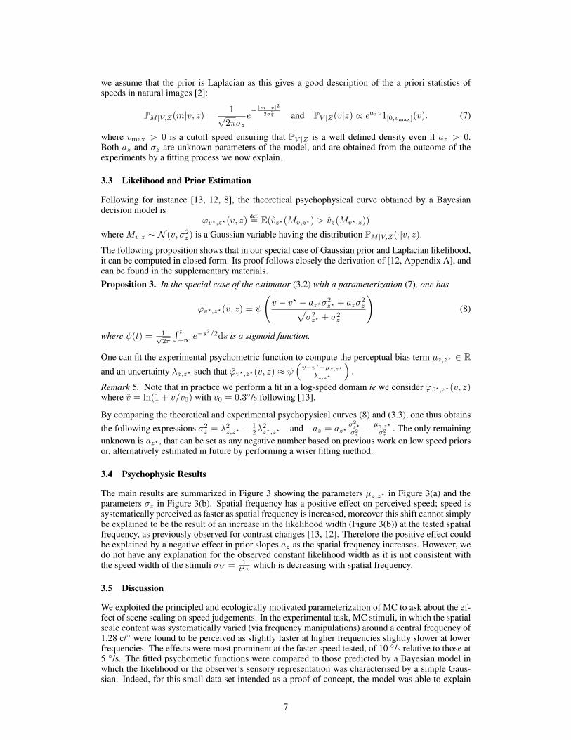
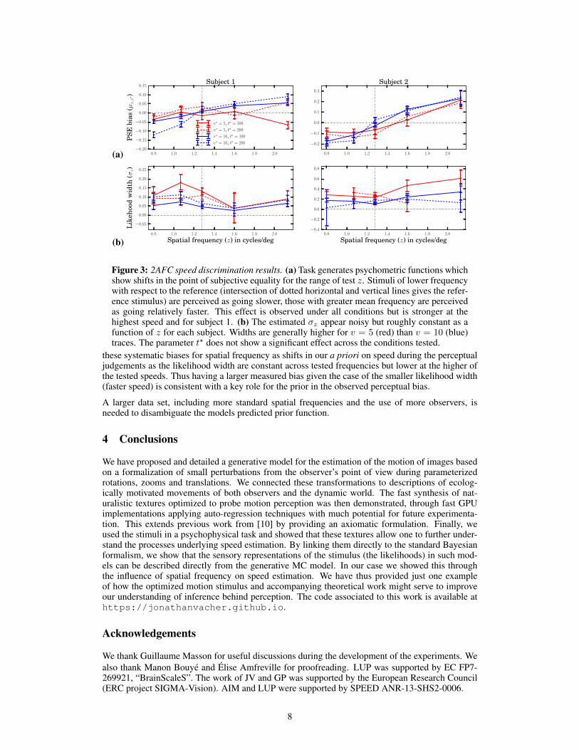
The main results are summarized in Figure 3 showing the parameters µz,z? in Figure 3(a) and theparameters σz in Figure 3(b). Spatial frequency has a positive effect on perceived speed; speed issystematically perceived as faster as spatial frequency is increased, moreover this shift cannot simplybe explained to be the result of an increase in the likelihood width (Figure 3(b)) at the tested spatialfrequency, as previously observed for contrast changes [13, 12]. Therefore the positive effect couldbe explained by a negative effect in prior slopes az as the spatial frequency increases. However, wedo not have any explanation for the observed constant likelihood width as it is not consistent withthe speed width of the stimuli σV = 1
t?z which is decreasing with spatial frequency.
3.5 Discussion
We exploited the principled and ecologically motivated parameterization of MC to ask about the ef-fect of scene scaling on speed judgements. In the experimental task, MC stimuli, in which the spatialscale content was systematically varied (via frequency manipulations) around a central frequency of1.28 c/◦ were found to be perceived as slightly faster at higher frequencies slightly slower at lowerfrequencies. The effects were most prominent at the faster speed tested, of 10 ◦/s relative to those at5 ◦/s. The fitted psychometic functions were compared to those predicted by a Bayesian model inwhich the likelihood or the observer’s sensory representation was characterised by a simple Gaus-sian. Indeed, for this small data set intended as a proof of concept, the model was able to explain
7
(a) 0.8 1.0 1.2 1.4 1.6 1.8 2.0−0.20
−0.15
−0.10
−0.05
0.00
0.05
0.10
0.15
PSE
bias
(µz,z∗ )
Subject 1
v∗ = 5, t∗ = 100
v∗ = 5, t∗ = 200
v∗ = 10, t∗ = 100
v∗ = 10, t∗ = 200
0.8 1.0 1.2 1.4 1.6 1.8 2.0
−0.2
−0.1
0.0
0.1
0.2
0.3
Subject 2
(b)0.8 1.0 1.2 1.4 1.6 1.8 2.0
Spatial frequency (z) in cycles/deg
−0.05
0.00
0.05
0.10
0.15
0.20
0.25
Lik
ehoo
dw
idth
(σz)
0.8 1.0 1.2 1.4 1.6 1.8 2.0
Spatial frequency (z) in cycles/deg
−0.4
−0.2
0.0
0.2
0.4
0.6
0.8
Figure 3: 2AFC speed discrimination results. (a) Task generates psychometric functions whichshow shifts in the point of subjective equality for the range of test z. Stimuli of lower frequencywith respect to the reference (intersection of dotted horizontal and vertical lines gives the refer-ence stimulus) are perceived as going slower, those with greater mean frequency are perceivedas going relatively faster. This effect is observed under all conditions but is stronger at thehighest speed and for subject 1. (b) The estimated σz appear noisy but roughly constant as afunction of z for each subject. Widths are generally higher for v = 5 (red) than v = 10 (blue)traces. The parameter t? does not show a significant effect across the conditions tested.
these systematic biases for spatial frequency as shifts in our a priori on speed during the perceptualjudgements as the likelihood width are constant across tested frequencies but lower at the higher ofthe tested speeds. Thus having a larger measured bias given the case of the smaller likelihood width(faster speed) is consistent with a key role for the prior in the observed perceptual bias.
A larger data set, including more standard spatial frequencies and the use of more observers, isneeded to disambiguate the models predicted prior function.
4 Conclusions
We have proposed and detailed a generative model for the estimation of the motion of images basedon a formalization of small perturbations from the observer’s point of view during parameterizedrotations, zooms and translations. We connected these transformations to descriptions of ecolog-ically motivated movements of both observers and the dynamic world. The fast synthesis of nat-uralistic textures optimized to probe motion perception was then demonstrated, through fast GPUimplementations applying auto-regression techniques with much potential for future experimenta-tion. This extends previous work from [10] by providing an axiomatic formulation. Finally, weused the stimuli in a psychophysical task and showed that these textures allow one to further under-stand the processes underlying speed estimation. By linking them directly to the standard Bayesianformalism, we show that the sensory representations of the stimulus (the likelihoods) in such mod-els can be described directly from the generative MC model. In our case we showed this throughthe influence of spatial frequency on speed estimation. We have thus provided just one exampleof how the optimized motion stimulus and accompanying theoretical work might serve to improveour understanding of inference behind perception. The code associated to this work is available athttps://jonathanvacher.github.io.
Acknowledgements
We thank Guillaume Masson for useful discussions during the development of the experiments. Wealso thank Manon Bouye and Elise Amfreville for proofreading. LUP was supported by EC FP7-269921, “BrainScaleS”. The work of JV and GP was supported by the European Research Council(ERC project SIGMA-Vision). AIM and LUP were supported by SPEED ANR-13-SHS2-0006.
8
References[1] Adelson, E. H. and Bergen, J. R. (1985). Spatiotemporal energy models for the perception of
motion. Journal of Optical Society of America, A., 2(2):284–99.[2] Dong, D. (2010). Maximizing causal information of natural scenes in motion. In Ilg, U. J. and
Masson, G. S., editors, Dynamics of Visual Motion Processing, pages 261–282. Springer US.[3] Doretto, G., Chiuso, A., Wu, Y. N., and Soatto, S. (2003). Dynamic textures. International
Journal of Computer Vision, 51(2):91–109.[4] Field, D. J. (1987). Relations between the statistics of natural images and the response properties
of cortical cells. J. Opt. Soc. Am. A, 4(12):2379–2394.[5] Galerne, B. (2011). Stochastic image models and texture synthesis. PhD thesis, ENS de Cachan.[6] Galerne, B., Gousseau, Y., and Morel, J. M. (2011). Micro-Texture synthesis by phase random-
ization. Image Processing On Line, 1.[7] Gregory, R. L. (1980). Perceptions as hypotheses. Philosophical Transactions of the Royal
Society B: Biological Sciences, 290(1038):181–197.[8] Jogan, M. and Stocker, A. A. (2015). Signal integration in human visual speed perception. The
Journal of Neuroscience, 35(25):9381–9390.[9] Nestares, O., Fleet, D., and Heeger, D. (2000). Likelihood functions and confidence bounds for
total-least-squares problems. In IEEE Conference on Computer Vision and Pattern Recognition.CVPR 2000, volume 1, pages 523–530. IEEE Comput. Soc.
[10] Sanz-Leon, P., Vanzetta, I., Masson, G. S., and Perrinet, L. U. (2012). Motion clouds: model-based stimulus synthesis of natural-like random textures for the study of motion perception. Jour-nal of Neurophysiology, 107(11):3217–3226.
[11] Simoncini, C., Perrinet, L. U., Montagnini, A., Mamassian, P., and Masson, G. S. (2012). Moreis not always better: adaptive gain control explains dissociation between perception and action.Nature Neurosci, 15(11):1596–1603.
[12] Sotiropoulos, G., Seitz, A. R., and Series, P. (2014). Contrast dependency and prior expecta-tions in human speed perception. Vision Research, 97(0):16 – 23.
[13] Stocker, A. A. and Simoncelli, E. P. (2006). Noise characteristics and prior expectations inhuman visual speed perception. Nature Neuroscience, 9(4):578–585.
[14] Unser, M. and Tafti, P. (2014). An Introduction to Sparse Stochastic Processes. CambridgeUniversity Press, Cambridge, UK. 367 p.
[15] Unser, M., Tafti, P. D., Amini, A., and Kirshner, H. (2014). A unified formulation of gaus-sian versus sparse stochastic processes - part II: Discrete-Domain theory. IEEE Transactions onInformation Theory, 60(5):3036–3051.
[16] Wei, L. Y., Lefebvre, S., Kwatra, V., and Turk, G. (2009). State of the art in example-basedtexture synthesis. In Eurographics 2009, State of the Art Report, EG-STAR. Eurographics Asso-ciation.
[17] Wei, X.-X. and Stocker, A. A. (2012). Efficient coding provides a direct link between priorand likelihood in perceptual bayesian inference. In Bartlett, P. L., Pereira, F. C. N., Burges, C.J. C., Bottou, L., and Weinberger, K. Q., editors, NIPS, pages 1313–1321.
[18] Weiss, Y. and Fleet, D. J. (2001). Velocity likelihoods in biological and machine vision. In InProbabilistic Models of the Brain: Perception and Neural Function, pages 81–100.
[19] Weiss, Y., Simoncelli, E. P., and Adelson, E. H. (2002). Motion illusions as optimal percepts.Nature Neuroscience, 5(6):598–604.
[20] Xia, G. S., Ferradans, S., Peyre, G., and Aujol, J. F. (2014). Synthesizing and mixing stationarygaussian texture models. SIAM Journal on Imaging Sciences, 7(1):476–508.
[21] Young, R. A. and Lesperance, R. M. (2001). The gaussian derivative model for spatial-temporalvision: II. cortical data. Spatial vision, 14(3):321–390.
9