biomechanical modeling of ray pectoral fins to inform the

Biomechanical modeling of ray pectoral fins

to inform the design of AUV propulsion systems

A Dissertation Presented to the

Faculty of the School of Engineering and Applied Science

University of Virginia

In Partial Fulfillment

of the Requirements for the Degree of

Doctor of Philosophy

Mechanical and Aerospace Engineering

Robert Scott French Russo

December 2012

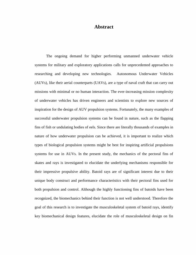
Abstract

The ongoing demand for higher performing unmanned underwater vehicle

systems for military and exploratory applications calls for unprecedented approaches to

researching and developing new technologies. Autonomous Underwater Vehicles

(AUVs), like their aerial counterparts (UAVs), are a type of naval craft that can carry out

missions with minimal or no human interaction. The ever-increasing mission complexity

of underwater vehicles has driven engineers and scientists to explore new sources of

inspiration for the design of AUV propulsion systems. Fortunately, the many examples of

successful underwater propulsion systems can be found in nature, such as the flapping

fins of fish or undulating bodies of eels. Since there are literally thousands of examples in

nature of how underwater propulsion can be achieved, it is important to realize which

types of biological propulsion systems might be best for inspiring artificial propulsions

systems for use in AUVs. In the present study, the mechanics of the pectoral fins of

skates and rays is investigated to elucidate the underlying mechanisms responsible for

their impressive propulsive ability. Batoid rays are of significant interest due to their

unique body construct and performance characteristics with their pectoral fins used for

both propulsion and control. Although the highly functioning fins of batoids have been

recognized, the biomechanics behind their function is not well understood. Therefore the

goal of this research is to investigate the musculoskeletal system of batoid rays, identify

key biomechanical design features, elucidate the role of musculoskeletal design on fin

kinematics and hydrodynamics, and to apply the lessons learned to the design of AUV

propulsion systems.

Computerized Tomography (CT) scans of the cownose ray (Rhinoptera bonasus)

and Atlantic ray (Dasyatis sabina) skeletons reveal a complex system of cartilaginous

joints and segments that provide for the support structure of batoid fins. Features of the

skeletal design believed to be important for kinematics and propulsion were identified. A

biomechanical model of the skeletal structure was developed to simulate ray swimming

kinematics and uncover the role of skeletal design on kinematics. The biomechanical

model was then interfaced with an advanced panel method Computational Fluid

Dynamics (CFD) model to establish a link between the skeletal structure and

hydrodynamic performance, and an investigation into the role of skeletal design on

hydrodynamics was conducted. Lastly, the applicability of skeletal design features of

biology to the design of AUV propulsion systems was explored through the design,

fabrication, and testing of bio-inspired artificial pectoral fin skeletons.

The development of the biomechanical model with fluid-structure interaction can

be used as a tool for transferring the biological design principles of ray fins to the design

of artificial systems for AUV propulsion. Ultimately, the objective of this work was to

establish an interface between biology and engineering to aid in the development of next

generation AUV technology. The present study introduced an approach of first analyzing

the biomechanics of ray pectoral fins, gaining knowledge of how the real biological

system works through fluid-structure modeling, then using this new knowledge to drive

the design of simplified artificial versions of ray pectoral fins for underwater propulsion.

The latter was done to test whether or not the biomechanical design approach of pectoral

fin propulsion systems found in nature could be an effective approach for the design of

artificial fins, as well as to learn if the form and function relationships revealed through

computational modeling can hold for simplified, artificial structures, that could be used

for propulsions and control of next generation AUVs.

i

Acknowledgements

I have had an extremely fulfilling and positive experience as a graduate student

and would like to acknowledge several individuals who have been a part of journey. I

would like to thank my fellow graduate students and lab mates Nic Fiorentino, Geoff

Handsfield, Chris Zirker, Bahar Sharifi, and Mike Rehorn of the Multi-scale Muscle

Mechanics lab for their support and feedback along the way. I would like to acknowledge

Shawn Russell for his help in creating LabView programs and setting up and configuring

experimental hardware. I would like to thank Trevor Kemp and Joe Zhu for offering their

advice on fabrication techniques and collaborating on research results. I would like to

thank Keith Moored for sharing his CFD MATLAB code and modeling expertise which

was essential in my research. I would also like to acknowledge undergraduate Kyle

Chadwick for his invaluable assistance and enthusiasm. I would like to thank Mehdi

Saadat for his willingness to always discuss our progress on ray modeling and for sharing

new ideas. I would also like to acknowledge Frank Fish for providing insight into ray

swimming from a biological perspective and for providing data that provided a

foundation for my work. I would also like to thank Hossein Haj-Hariri for providing

insight into the hydrodynamics of ray swimming help on interpreting results. I would like

to thank Silvia Blemker and Hilary Bart-Smith for their guidance and oversight during

my time as a graduate student, and for helping me navigate my way through the PhD

program. I greatly appreciate the freedom I was given to define my own research path

and positive feedback and encouragement I received proved to be invaluable in helping

me progress in my studies. I could not have been more pleased with my faculty advisors.

ii

I would like to thank my mother and father for their support over the years as well as my

brothers, Alex, Chris, and Matthew. I would also like to thank my four month old

daughter, Sadie, who most likely without any knowledge, has helped me get through the

days leading up to my defense. I would also like to extend special thanks to my wife,

Kristin, who has been with me all the way, supporting me, encouraging me, and sharing

in my success, as I have shared in hers. I am truly blessed to have her in my life and

could not have gotten this far without her.

iii

Contents Acknowledgements………………………………………………………………………...i

List of figures………………………………………………………………………….….vi

List of tables…………………………………………………………………………...….ix

Nomenclature……………………………………………………………………………...x

1 Project Overview

1.1 Introduction………………………………………………………………………....…1

1.2 Background of AUV technology and state-of-the-art research…………………….…3

1.3 Biological Foundation………………………………………………………………....6

1.4 Hydrodynamic Background……………………………………………………….......7

1.5 Structural Background (biological and artificial)…………………………………......8

1.6 Summary……………………………………………………………………………..10

2 Biomechanical model of skeletal architecture and kinematics……………….…..…....12

2.1 Materials and methods

2.1.1 Ray species selection…………………………………………….…….......13

2.1.2 CT Investigation…………………………………………………………....14

2.1.3 Biomechanical model development……………………….…………….…16

2.1.4 in vivo ray swimming comparison……………………………….…..….…19

2.1.5 Biomaterial testing………………………………………………………....23

2.1.6 Perturbation studies……………………………………….……………......25

2.2 Results

2.2.1 Skeletal parameter measurements………………….………………..…..…27

iv

2.2.2 Validation………………………………………………………………..…27

2.2.3 Biomaterial strain thresholds………………………………………….…...30

2.2.4 Perturbation study results…………………………………………………..32

2.3 Discussion…………………………………………………………………..………..36

3 Fluid Structure Interaction (FSI)………………………………………………….……40


3.1.1 Unsteady panel method………………………………………………....….41

3.1.2 Joint displacement to panel node displacement mapping……………...…..42

3.1.3 Biomechanical model and CFD model integration…………………….…..44

3.1.4 Hydrodynamic performance metrics………………………………..…..….46

3.1.5 Perturbation studies (Hydrodynamic test matrix)……………………….....48

3.2 Results (perturbation study hydrodynamics)

3.2.1 Perturbation study results for in vivo prescribed motions…………….…...50

3.2.2 Perturbation study 1 results for full test matrix……………………….…...58

3.2.3 Perturbation study 2 results for full test matrix………………………..…..66

3.3 Discussion………………………………………………………………………..…..67

4 Parameterized modeling of ray-like skeletal structures………………………...…...…71


4.1.1 Parameterized model development……………………………………...…72

4.1.2 Inter-radial joint pattern (IRJP) angle study………...………………….….74

4.1.3 Fanning angle study………………………………………..…….…….…..76

4.1.4 Simplified structure IRJP angle study………………………………..….....77

4.2 Results – (parameterized modeling FSI)

v

4.2.1 IRJP angle study results………………………………………...………….78

4.2.2 Fanning angle study results………………………………………...…..…..87

4.2.3 Simplified structure IRJP angle study results………………………...……89

4.3 Discussion………………………………………………………………………..…..93

5 Bio-inspired design of artificial pectoral fin skeletal system………………………......96


5.1.1 Artificial structure design and actuation platform……………………....…97

5.1.2 Structure motion control…………………………………………....….....100

5.1.3 Hydrodynamic experimentation……………………………………..…....104

5.2 Results – (artificial structure testing)………………………………………….…....107

5.3 Discussion……………………………………………………………...………..….109

6 Conclusions and future work…………………………………………………………112

vi

List of Figures

1.1 Global Outlook on study……………….………………………………………...……4

1.2 Current state-of-the-art AUVs…………………………………………………..….…5

1.3 Underwater photographs of the Manta-ray, cownose ray, and Atlantic sting-ray.…....6

2.1 Reconstructed CT scans of the cownse and Atlantic ray………………………….....15

2.2 Biomechanical model description…………………………………………….….…..17

2.3 in vivo swimming model comparison for the Atlantic ray…………………….….…20

2.4 in vivo swimming model comparison for the cownose ray……………….…..….….21

2.5 Specimen preparation for deformed fin CT scanning…………………………..…....22

2.6 Biomaterial sample preparation and test setup……………………………….……...24

2.7 Skeletal morphology perturbation study method - perturbation study 1 and 2….…...26

2.8 Results of deformed fin CT scans…………………………………………………....30

2.9 Biomaterial strain threshold test results………………………………………..….…31

2.10 Cownose v. Atlantic ray gait swapping results……………………………….….…33

2.11 Perturbation study 1 strain-displacement results………………………………..….34

2.12 Perturbation study strain-displacement results…………………………………......35

3.1 Biomechanical model and CFD model integration method……………………….....44

3.2 Computational flow of interfaced models……………………………………...….…45

3.3 Perturbation study performance comparisons for in vivo motions…………....……..51

3.4 Thrust distribution plots for perturbation study 1……………………………………54

3.5 Thrust distribution plots for perturbation study 2……………………………………55

3.6 Leading edge (LE) & trailing edge (TE) angle analysis for perturbation study 1...…57

3.7 Thrust production results for perturbation study 1 full test matrix…………...…..….59

vii

3.8 Propulsive efficiency results for perturbation study 1 full test matrix….………..…..60

3.9 Cruising economy results for perturbation study 1 full test matrix…………….……61

3.10 Strain predictions for perturbation study 1 full test matrix…………………….......62

3.11 Variable gait efficiency plots for the cownose ray……………………………...….64

3.12 Leading edge & trailing edge pitch angle v. strain for perturbation study………....65

3.13 Thrust and efficiency plots perturbation study 2 full test matrix………………..….67

3.14 Strain predictions for perturbation study 1 full test matrix…………….……….….68

4.1 Illustration of parameterized modeling approach…………....…………….…….…..74

4.2 Inter-radial joint pattern (IRJP) angle study method…………………………….…..75

4.3 Fanning angle study method………………………………………………………....76

4.4 Simplified structure IRJP angle study method……………………………………….77

4.5 IRJP angle study results for in vivo prescribed motions of the cownose ray….....….79

4.6 Thrust distribution plots for IRJP angle study………………………….…….……...80

4.7 Fin pitch angles v. IRJP angle v. thrust and efficiency………………………………81

4.8 Thrust production results for IRJP angle full test matrix…………………….......…..83

4.9 Propulsive efficiency results for IRJP angle full test matrix…………………...…....84

4.10 Cruising economy results for IRJP angle full test matrix………………….........….85

4.11 Fin pitch angle v. IRJP angle v. strain for full test matrix…………………...…..…87

4.12 Fanning angle study results for in vivo prescribed motions of the cownose ray...…88

4.13 Simplified IRJP angle study results for in vivo motions of the cownose ray............90

4.14 Fin pitch angles v. IRJP angle v. thrust and efficiency - simple v. complex fin…...92

5.1 Artificial musculoskeletal system design………………………………………..…...98

5.2 Artificial structure and actuation system integration………………………..…..….101

5.3 Control signal acquisition method using biomechanical model………………..…..103

5.4 Hydrodynamic experimentation setup…………………………………………..….105

viii

5.5 Artificial structure IRJP angle experimental test method………………….….…....107

5.7 Artificial structure IRJP angle experimental results…………………………….….108

ix

List of Tables

2.1 Cartilage structure data for the cownose and Atlantic ray………………….………..28

2.2 In vivo kinematic data for the cownose and Atlantic ray……………………………29

3.2 Test matrix for perturbation study 1..…………………………………………..……49

3.3 Test matrix for perturbation study 2………………………………………….….…..49

x

Nomenclature

𝜃𝑟𝑠 Joint angle matrix

r Radial element position index

s Radial segment position index

𝜃𝑚𝑎𝑥 Maximum joint angle (i.e., amplitude of oscillation)

𝛷 Angular phase between adjacent radial elements

𝛹 Angular phase between connecting radial segments

𝜔 Frequency of oscillation

𝑡 time in seconds

δ Joint angle offset for asymmetric flapping

𝑁𝑐 Chord-wise traveling wave number

𝑅 Total number of radial elements

𝑁𝑠 Span-wise traveling wave number

𝑆 Total number of radial segments of the longest radial element

𝑽𝑟𝑠 Joint displacement field

𝑼𝑟𝑠 Joint position vector field

𝑥𝑟𝑠 Joint x-coordinate

xi

𝑦𝑟𝑠 Joint y-coordinate

𝑧𝑟𝑠 Joint z-coordinate

𝐿𝑟𝑠 Radial segment length matrix

𝛽𝑟𝑠 Radial segment transverse angle matrix

𝜀𝑟𝑠 Adjacent radial strain matrix

𝑸𝑖𝑗 Panel node position vector field

i Chord-wise panel node position index

j Span-wise panel node position index

𝜦𝑖𝑗𝑚 Barycentric coordinate matrix

m Triangular element identification index

𝑁𝑚 Triangular element node position matrix

�̂�𝑥 Basis vector along x

�̂�𝑦 Basis vector along y

�̂�𝑧 Basis vector along z

𝒖1𝒎 Joint position vector corresponding to node 1 of element m


xii


𝐹𝑥 Hydrodynamic force along x

𝑇 Thrust

𝑎 Acceleration

𝑛 Simulation time step index

𝑀𝑟𝑎𝑦 Body mass of ray

𝑉∞ Free stream velocity

𝛥𝑡 Simulation time step duration

𝑋 Vector of body positions along x

f Gait cycle frequency

𝑇𝑎𝑣𝑔 Average thrust

𝑉𝑎𝑣𝑔 Average velocity

𝑃𝑎𝑣𝑔 Average hydrodynamic power

𝜂𝑝 Propulsive efficiency

𝑐𝑦𝑐𝑙𝑒0.5 Half-cycle period index

𝑁𝑠𝑡𝑒𝑝 Number of time steps per cycle

𝐸𝑠𝑠 Steady state economy

xiii

𝑉𝑠𝑠 Steady state velocity

𝑃𝑠𝑠 Cycle average hydrodynamic power at steady state

𝑝𝐿𝐸𝑗 Vector of leading edge pitch angle values

𝑝𝑇𝐸𝑗 Vector of trailing edge pitch angle values

𝑷𝑖𝑗 Panel node position vector field

𝛾𝑠 IRJP angle vector

𝛾𝑚𝑎𝑥 Maximum IRJP angle

𝜁𝑟 Fanning angle vector

𝜁𝑚𝑎𝑥 Maximum fanning angle

𝚾 Matrix containing planform shape vertices

𝑮𝑟𝑠 Joint position vector field for parameterized structure

∆𝑥 Chord-wise joint spacing

∆𝑦 Span-wise joint spacing

𝐿𝑐ℎ𝑜𝑟𝑑 Fin chord length

𝐿𝑠𝑝𝑎𝑛 Fin span length

𝛺2 Two-dimensional rotation matrix

𝛺3 Three-dimensional rotation matrix

xiv

𝐼3 Three-dimensional identity matrix

𝐸𝑟𝑠 Moment arm orientation matrix

𝑴𝑟𝑠 Cable attachment point position vector field

𝑚𝑟𝑠 Moment arm length matrix

𝐶𝑟𝑠 Cable travel magnitude matrix

𝐴𝑟𝑠𝑒𝑟𝑣𝑜 Servo amplitude vector

1

Chapter 1

Project Overview

1.1 Introduction

The shift toward developing unmanned vehicles for military and exploratory

applications has motivated research of bio-inspired technologies in recent years.

Autonomous Underwater Vehicles (AUVs) represent a class of unmanned vehicle

intended for naval and research applications. The increasing demand in vehicle

performance has driven engineers and scientists to explore novel avenues in the research

and development of AUV propulsion systems [1][20]. Fortunately, nature has provided a

source of inspiration, with thousands of examples of successful propulsion systems found

in fish and marine mammals. As such, bioinspired AUVs, or BAUVs, is a particular class

of underwater vehicle that attempts to take advantage of propulsion principles employed

by nature. In particular, the pectoral-fin-based propulsion systems found in skates and

rays is an attractive design model for BAUVs. The order of rays, Myliobatiformes, is of

significant interest due to their unique body construct and performance characteristics.

Myliobatiformes (i.e., batoid rays) exhibit extreme dorsiventral flattening of their bodies

with diminished tails leaving the pectoral fins as their only means of generating

propulsion in the majority of species [1]. They have a pair of pectoral fins attached to a

central body, which remains relatively rigid during swimming. The fins serve as both the

propulsive mechanisms as well as the control surfaces of the ray. The integration of

2

propulsion and control into a pair of pectoral fins, combined with a center positioned

rigid body, make batoid rays an attractive model for a BAUV design.

In addition to the desirable body-fin platform design, the hydrodynamic

performance exhibited by batoids is superior to that of state of the art AUVs to date [2].

Some of the sought after performance characteristics include:

1) Superior low speed maneuverability

2) High bursts of acceleration from rest

3) Station keeping ability

4) Propulsion and control blended into one system (i.e., the fin)

5) Low noise signature associated with propulsion system

6) High propulsive efficiency and cruising endurance

Many of these performance attributes are achieved solely through the use of the

ray’s pectoral fins [4][5], making it clear that successful pectoral fin propulsion systems

are possible in nature. Understanding the biomechanical design principles of real,

biological ray fins, is an essential step in establishing a foundation for informing the

design of artificial pectoral fin systems for use in AUVs.

Research in the area of bioinspired engineering is a multidisciplinary subject

requiring experts from both the physical and life sciences [2,20]. In the case of

developing BAUVs, both biologists and engineers offer unique perspectives on how to

approach this problem. The musculoskeletal system found in rays is a highly complex

mechanical system that is capable of deforming to extreme shapes during swimming and

3

maneuvering. Biologists and zoologists have observed and documented the swimming

characteristics of batoids in the past [3,4,5,6,9,14], and some research into the

musculoskeletal anatomy was performed [4,8]. However, focus is limited to explain how

the musculoskeletal system functions mechanically to achieve the motions seen in nature

and create propulsion. On the other hand, engineers have designed and built bioinspired

artificial pectoral fin systems, and carried out research into their potential for use in

AUVs [10,12,13,15,21], but the current systems fall short in their ability to fully

reproduce the performance characteristics of pectoral-fin-based swimmers found in

nature.

Analyzing the musculoskeletal biomechanics of batoid rays quantitatively will

help uncover and elucidate the biological design principles behind their propulsion. The

goals of this dissertation are therefore to 1) establish an interface between biology

and engineering through biological investigation and biomechanical modeling, 2)

gain an understanding of the biological design principles behind pectoral-fin-based

propulsion by integrating the biomechanical modeling with Computational Fluid

Dynamics (CFD) modeling, and 3) investigate the applicability of the biological

principles to the design and performance of artificial pectoral fin systems for use in

AUVs.

1.2 Background of AUV technology and state-of-the-art research

Contemporary AUVs in service today are typically scaled down versions of

larger, manned, vehicles such as naval submarines or submersible rescue vehicles [2].

4

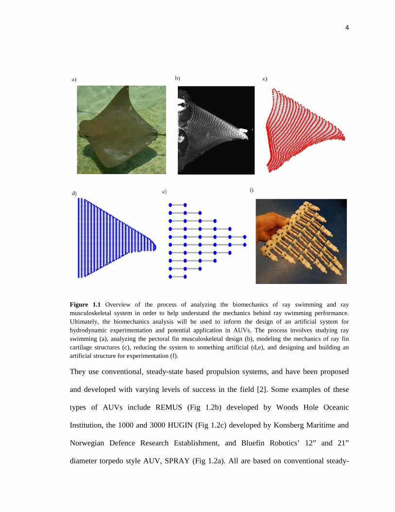
Figure 1.1 Overview of the process of analyzing the biomechanics of ray swimming and ray musculoskeletal system in order to help understand the mechanics behind ray swimming performance. Ultimately, the biomechanics analysis will be used to inform the design of an artificial system for hydrodynamic experimentation and potential application in AUVs. The process involves studying ray swimming (a), analyzing the pectoral fin musculoskeletal design (b), modeling the mechanics of ray fin cartilage structures (c), reducing the system to something artificial (d,e), and designing and building an artificial structure for experimentation (f).

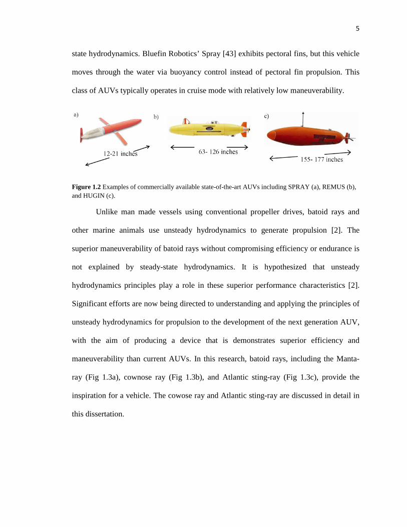
They use conventional, steady-state based propulsion systems, and have been proposed

and developed with varying levels of success in the field [2]. Some examples of these

types of AUVs include REMUS (Fig 1.2b) developed by Woods Hole Oceanic

Institution, the 1000 and 3000 HUGIN (Fig 1.2c) developed by Konsberg Maritime and

Norwegian Defence Research Establishment, and Bluefin Robotics’ 12” and 21”

diameter torpedo style AUV, SPRAY (Fig 1.2a). All are based on conventional steady-

5

state hydrodynamics. Bluefin Robotics’ Spray [43] exhibits pectoral fins, but this vehicle

moves through the water via buoyancy control instead of pectoral fin propulsion. This

class of AUVs typically operates in cruise mode with relatively low maneuverability.

Figure 1.2 Examples of commercially available state-of-the-art AUVs including SPRAY (a), REMUS (b), and HUGIN (c).

Unlike man made vessels using conventional propeller drives, batoid rays and

other marine animals use unsteady hydrodynamics to generate propulsion [2]. The

superior maneuverability of batoid rays without compromising efficiency or endurance is

not explained by steady-state hydrodynamics. It is hypothesized that unsteady

hydrodynamics principles play a role in these superior performance characteristics [2].

Significant efforts are now being directed to understanding and applying the principles of

unsteady hydrodynamics for propulsion to the development of the next generation AUV,

with the aim of producing a device that is demonstrates superior efficiency and

maneuverability than current AUVs. In this research, batoid rays, including the Manta-

ray (Fig 1.3a), cownose ray (Fig 1.3b), and Atlantic sting-ray (Fig 1.3c), provide the

inspiration for a vehicle. The cowose ray and Atlantic sting-ray are discussed in detail in

this dissertation.

6

Figure 1.3 Underwater clips of the Manta-ray (a), cownose ray (b), and Atlantic stingray (c).

1.3 Biological Foundation

Batiod rays are cartilaginous fishes having dorsaventrally flattened bodies with

pectoral fins that are greatly expanded and fused to the head [5], and can range in

planform shape from circular to rhomboidal [16]. Their pectoral fins are highly modified

and are often used as the primary locomotor propulsors capable of deforming to various

shapes during ray swimming [4,17]. The fins are supported by highly complex skeletal

structures which consist of an array of serially repeating cartilaginous elements composed

of cartilage segments connected in series by joints [8] (Fig 2.1c). These radial elements

originate at the pectoral girdle, or fin root, and extend outward to the edge of the fin and

repeat along the ray body [8]. Mechanical connections between radial elements are found

in the form of adjacent radial cross-bracing or soft tissue connective membrane [8].

Though these cartilaginous joints, segments, and adjacent radial connections are common

components shared between all ray species, the assembly of these components varies

considerably. Schaefer and Summers, 2005, identified such morphological differences

(i.e., morphological parameters) reporting variations in radial element length and

orientation in association with planform shape, the presence of cross-bracing versus soft

7

tissue adjacent radial connections, and variations in internal joint patterns between radial

elements [8].

Pectoral-fin-based locomotion is classified within two extremes of swimming

style, undulatory (rajiform) and oscillatory (mobuliform) [1,3,9,16,19]. With respect to

ray locomotion, oscillation typically refers to high-amplitude flapping motion with

significant span-wise curvature [15,4,12], and undulation refers to motion in which a

wave propagates down the pectoral fin from anterior to posterior [14] with a frequency of

one or higher [9]. Many rays, however, fall somewhere between these two extremes and

therefore cannot clearly be categorized as undulators or oscillators [5]. Rosenberger, et al.

in 2001 developed a swimming mode continuum, which categorizes all forms of pectoral-

fin-based locomotion by the number of undulatory waves (i.e., undulatory wave number)

that travel along the chord of the fin [5]. In species that display larger oscillation, such as

the manta-ray, undulation in the span-direction of the fin is also observed. Consequently,

a key objective of the present research was to understand how the underlying skeletal

architecture affects the observed swimming kinematics of batoid rays.

1.4 Hydrodynamics background

As fish and other marine wildlife are observed to flap or undulate their fins to

produce thrust and lift [1,3,4,5,9], significant effort has been directed towards

investigating the hydrodynamics of heaving and pitching airfoils to begin understanding

how this form of propulsion works [22]. High propulsive efficiencies, up to 87%, were

reported by Anderson et al [22] who studied the vortices that develop from pitching and

heaving airfoils. It was further identified that the phase between heaving and angular

8

twisting motions is an important factor in optimizing the motion for hydrodynamic

efficiency [15,28,30,31,32]. The heaving and angular twisting motions can be considered

simplified reproductions of the oscillatory and undulatory motions of ray fins. The

importance of vortex shedding and flapping frequency and amplitude have been

demonstrated [29,30]. In particular, Lewin and Haj-Hariri [28] showed that the frequency

of heaving motion and the interaction between leading and trailing edge vortices play

important roles in hydrodynamic efficiency, and that these principles extend to

undulatory swimming also [30]. As the motion of ray pectoral fins is much more complex

than a heaving and pitching airfoil, Heathcote et al [23] studied the hydrodynamics of an

oscillating foil with passive flexibility. This study revealed that flexibility in the fin leads

to some span-wise curvature, which if smartly induced can increase thrust and propulsive

efficiency. Numerical modeling of flexible body hydrodynamics has been successfully

implemented and the benefits of fin flexion control were reinforced [32,33,34]. More

recently, the importance to the hydrodynamics of chord-wise traveling waves (shown by

Rosenberger, 2001 [5]) has been shown where chord-wise traveling wave motion is

important in wake structure formation and hydrodynamic performance [15,37,39].

1.5 Structural background (biological and artificial)

Many concepts for designing bio-inspired propulsion platforms have been

presented which replicate the motion of fish [44,45,46,47], dolphins [50,51], and eels

[48][49]. With respect to rays, artificial pectoral fin designs have become more refined

with actuators and active support structures that can better reproduce the motions seen in

9

nature. Moored and Bart-smith explored tensegrity beam based actuation systems as a

potential candidate for use in BAUVs with pectoral fin propulsion [10,12]. Incorporating

multiple tensegrity beams has been explored which allows for the dominant

characteristics of ray locomotion to be reproduced including oscillation, span-wise

curvature and undulatory motion through a phase delay between adjacent beams [10,36].

Furthermore, coupling an active beam with passive fin structures have also shown to be

effective in optimizing thrust production [15,23,36]. Additionally, prior work

investigating real biological specimens reveal that both active and passive mechanisms

are involved in fish and marine mammal propulsion [25,26,14,19]. Though much

improvement has been made in designing artificial pectoral fin support structures with

actuation potential, the current designs still fall short of being able to achieve the motions

observed in nature. To bridge this gap, the present research explores the mechanics of ray

pectoral-fin musculoskeletal systems, with the goal of using the results to inform next

generation AUV propulsors. The morphology behind these musculoskeletal systems is

believed to play an important role in the achievement of the fin kinematics required for

the optimal hydrodynamic performance. However, little work has been done to explain

the mechanics behind the functionality of ray pectoral fin musculoskeletal systems. If the

mechanisms that enable pectoral fin function can be described and understood, then the

lessons learned can be applied to the design of artificial pectoral fin systems to bridge the

performance gap between current artificial designs and the real biological systems.

10

1.6 Summary

In this dissertation, I investigated the biomechanics of rays in order to determine

how pectoral fin propulsion system functions to achieve its impressive performance

characteristics. This study demonstrates that the configuration of the underlying cartilage

structure is important in achieving fin kinematics that produces performance advantages.

The biomechanical/CFD integrated modeling approach uncovered the relationships

between the design of a given skeletal structure, fin kinematics, and underwater

propulsion. The results of this research demonstrate that fin skeletal design affects the

structural mechanics, as well as the fluid mechanics, of pectoral-fin-based propulsion

systems. Furthermore, it is experimentally shown that the biological design principles

observed in batoid rays can be leveraged in the design of artificial systems to achieve

gains in swimming performance.

The following chapters (2-5) explain the methods, results, and conclusions of this

work and discuss the contributions to both biology and engineering. Chapter 2 explains

the methods for examining the skeletal morphometry, identifying skeletal design

parameters, and developing a biomechanical kinematic model to explore the link between

skeletal design and locomotion. Chapter 3 introduces a fluid modeling component, in

which a method for interfacing the biomechanical model with a computational fluid

dynamics (CFD) model is introduced to complete the loop between skeletal design,

kinematics, and hydrodynamic performance. In chapter 4, a parameterized model is

introduced to quantify the effects of skeletal parameter manipulation on performance,

which leads to experimental work discussed in chapter 5 in which simplified versions or

ray skeletal structures are design, fabricated, and tested. The contributions of this work,

11

comparisons to other researchers who have conducted similar studies, and future work

are discussed in chapter 6.

12

Chapter 2

Biomechanical model of skeletal architecture and kinematics

The fins of batoid rays are composed of an array of cartilage segments connected

in series by joints to form finger-like structures called radial elements (Fig 2.1) [8], with

adjacent connections running chord-wise to hold the radial elements together. All rays

have these features, however the assembly of these components has been shown to vary

considerably [8]. For example, radial element lengths and orientations as well internal

joint patterns between radial elements have been shown to vary across different ray

species [8]. Though these variations in the skeletal design have been identified, it is

currently unclear how such variations affect ray locomotion. Therefore to address this

problem, we have examined the effect of three skeletal design parameters on fin

kinematics including 1) inter-radial joint pattern (IRJP), 2) fanning angle, and 3)

planform shape (Fig 2.1).

A numerical solution was developed to describe the motion of different ray

skeletal structures. Computational models were developed based on mathematical

descriptions of the motions of cartilage segments (both spatially and temporally) in order

to simulate how a real ray skeletal structure would have to operate in order to achieve the

motions of the whole fin observed in nature. Through this approach, the influence of

skeletal design parameters (i.e., IRJP, fanning angle, planform) on ray swimming

kinematics was examined. The computational approach was adopted because it allows for

the internal features of the ray skeleton (i.e., IRJP and fanning angle) to be decoupled

from the external features (i.e., planform). This ability enables the effects of planform

13

shape and internal cartilage arrangement to be studied independently, and allow

conditions to be tested through simulations that would be impossible to test

experimentally. The specific aims of this chapter were to: (i) develop a computational

biomechanical model to simulate how the ray skeletal structure would function to achieve

ray locomotion observed in nature, (ii) validate the model through in vivo ray swimming

comparison and CT imaging, and (iii) conduct perturbation studies to study how

variations in skeletal architecture and planform shape affect fin kinematics. The analysis

was carried out by quantifying differences in joint displacement and mechanical strain as

a function of the skeletal design parameters. The results show that the arrangement of

cartilage joints plays a role in determining the deformation characteristics of a given fin

structure, and further highlighted that the joint arrangement can be an effective method

for altering the structural deformation without additional structural strain. Ultimately,

insights gained from this work can be used to inform the mechanical design of artificial

pectoral fins for AUV propulsion systems.


2.1.1 Ray Species Selection

Two species of rays were selected for this study: Atlantic stingray (Dasyatis

Sabina, Fig 1.3c), and cownose ray (Rhinoptera bonasus, Fig 1.3b). Both the Atlantic and

cownose ray belong to the taxonomic group Batoidea [4]; however, they are at opposite

ends of the swimming mode continuum [5]. The cownose ray is considered to be an

oscillator and the Atlantic ray an undulator [5,8]. By choosing species that are

14

taxonomically related, but exhibit different swimming styles, the explanation of the

kinematic differences between the two species can be limited to only differences relating

pectoral fin skeletal morphology.

2.1.2 CT imaging of skeletal architecture

A series of Computed Tomography (CT) scans were taken to create a three-

dimensional (3D) reconstruction of the underlying cartilage structure of the Atlantic and

cownose rays (Fig. 2.1a,b). Scans were taken with their bodies flattened against the

scanning platform as in an in vivo rest position. The cownose ray specimen was

approximately 344mm in chord-length and 279mm in span, and the Atlantic ray

specimen was 343mm in chord-length and 162mm in span, where span is measured from

the body midline to the fin tip. The scans were taken along the span of each ray on a

Siemens Volume Zoom CT scanner, beginning at one fin tip and progressing over the

entire body to the other fin tip. Spiral protocols for data acquisitions with 100mAs,

120kV, 0.5 detector collimation at 0.5mm/sec table feeds and 1sec tube rotations were

used. All images were reconstructed in both soft tissue (U40u) and ultra-high resolution

(U90u) kernels. Three-dimensional reconstructions of the ray skeleton were digitally

rendered from the DICOM images of the CT scans using Osirix Imaging Software

(Advanced Open-Source PACS Workstation DICOM Viewer, www.osirix-viewer.com).

For each specimen, the three-dimensional location of each cartilage joint was digitized

based on the 3D reconstructions in Osirix (Fig. 2.1c,d). The connectivity between joints

in each radial also was recorded.

15

Figure 2.1 Reconstructed CT images of the Atlantic ray (a) and cownose ray (b) from the dorsal perspective to reveal the anatomical components of the skeleton; including radial segments, joints, and adjacent radial connective tissues. Skeletal morphometry was quantified by digitizing CT images and obtaining the coordinates of cartilage joint positions (c), (d) – green. Skeletal patterns were identified from the images including palnform (red), inter-radial joint pattern (IJRP) (blue), and fanning angle (c-magenta).

16

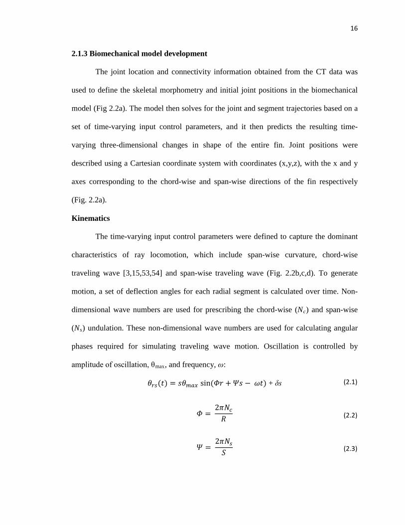
2.1.3 Biomechanical model development

The joint location and connectivity information obtained from the CT data was

used to define the skeletal morphometry and initial joint positions in the biomechanical

model (Fig 2.2a). The model then solves for the joint and segment trajectories based on a

set of time-varying input control parameters, and it then predicts the resulting time-

varying three-dimensional changes in shape of the entire fin. Joint positions were

described using a Cartesian coordinate system with coordinates (x,y,z), with the x and y

axes corresponding to the chord-wise and span-wise directions of the fin respectively

(Fig. 2.2a).

Kinematics

The time-varying input control parameters were defined to capture the dominant

characteristics of ray locomotion, which include span-wise curvature, chord-wise

traveling wave [3,15,53,54] and span-wise traveling wave (Fig. 2.2b,c,d). To generate

motion, a set of deflection angles for each radial segment is calculated over time. Non-

dimensional wave numbers are used for prescribing the chord-wise (Nc) and span-wise

(Ns) undulation. These non-dimensional wave numbers are used for calculating angular

phases required for simulating traveling wave motion. Oscillation is controlled by

amplitude of oscillation, θmax, and frequency, ω:

𝜃𝑟𝑠(𝑡) = 𝑠𝜃𝑚𝑎𝑥 sin(𝛷𝑟 + 𝛹𝑠 − 𝜔𝑡) + δs

𝛷 = 2𝜋𝑁𝑐𝑅

𝛹 = 2𝜋𝑁𝑠𝑆

(2.1)

(2.2)

(2.3)

17

Figure 2.2 Summary of model inputs including xy coordinates representing joint locations with joints represented as red dots and cartilage segments represented as gray line segments (a), Kinematic inputs and method for achieving spanwise curvature (b), non-dimensional wave numbers for chordwise traveling wave (i.e., undulation) (c) and spanwise traveling wave (d).

18

where ω = 2πf, and f is the frequency of oscillation. R and S are the total number of radial

elements and segments of the longest radial element, respectively. The indices r and s

denote the position of cartilage segment, s, relative to the fin root of radial element, r,

relative to the leading edge. Nc refers to the number of waves traveling along the chord of

the fin, while Ns is the span-wise traveling wave number. Both Nc and Ns are kinematic

variables used for calculating time independent angular phases Φ and Ψ to achieve

traveling wave motion. A scalar term, δ, is included for achieving asymmetric flapping

where any non-zero value of δ will result in a vertical shift in the y-axis of the deflection

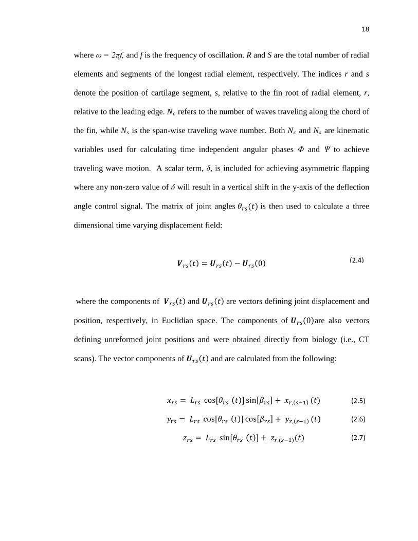
angle control signal. The matrix of joint angles 𝜃𝑟𝑠(𝑡) is then used to calculate a three

dimensional time varying displacement field:

𝑽𝑟𝑠(𝑡) = 𝑼𝑟𝑠(𝑡) − 𝑼𝑟𝑠(0)

where the components of 𝑽𝑟𝑠(𝑡) and 𝑼𝑟𝑠(𝑡) are vectors defining joint displacement and

position, respectively, in Euclidian space. The components of 𝑼𝑟𝑠(0)are also vectors

defining unreformed joint positions and were obtained directly from biology (i.e., CT

scans). The vector components of 𝑼𝑟𝑠(𝑡) and are calculated from the following:

𝑥𝑟𝑠 = 𝐿𝑟𝑠 cos[𝜃𝑟𝑠 (𝑡)] sin[𝛽𝑟𝑠] + 𝑥𝑟,(𝑠−1) (𝑡)

𝑦𝑟𝑠 = 𝐿𝑟𝑠 cos[𝜃𝑟𝑠 (𝑡)] cos[𝛽𝑟𝑠] + 𝑦𝑟,(𝑠−1) (𝑡)

𝑧𝑟𝑠 = 𝐿𝑟𝑠 sin[𝜃𝑟𝑠 (𝑡)] + 𝑧𝑟,(𝑠−1)(𝑡)

(2.5) (2.6) (2.7)

(2.4)

19

beginning with s = 2 and extending out along each radial element r. The matrices L and β

are radial segment length and transverse segment angle respectively, where the transverse

angle refers to the angle of the cartilage segment rs in the xy-plane relative to the x-axis.

The cartilage segments are represented as rigid bodies and joints are represented as hinge

joints constrained to a single rotational degree of freedom (Fig 2.2b). These kinematic

constraints are enforced by measuring the values of L and β for the fin at rest and holding

them constant. These two assumptions give rise to the system’s kinematic constraints and

are essential to solving the kinematics.

Strain and displacement analysis

In order to quantify the physical consequences of forcing a given structure to

perform different motions, the joint displacements and subsequent mechanical strain that

develops between adjacent radials was calculated (Fig. 2.1c – magenta) from the

following expression:

𝜀𝑟𝑠(𝑡) = �𝑼𝑟𝑠(𝑡) − 𝑼(𝑟+1),𝑠(𝑡) − 𝑼𝑟𝑠(0) + 𝑼(𝑟+1),𝑠(0)�

�𝑼𝑟𝑠(0) − 𝑼(𝑟+1),𝑠(0)�

for which all variables are calculated by the model using equations 2.4 through 2.7.

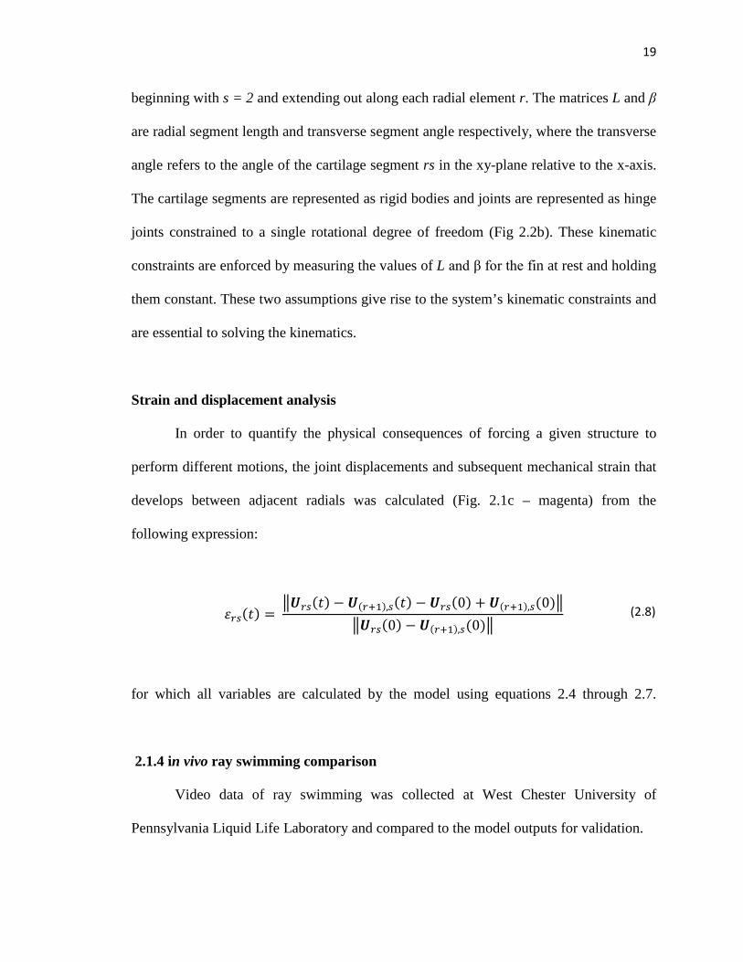
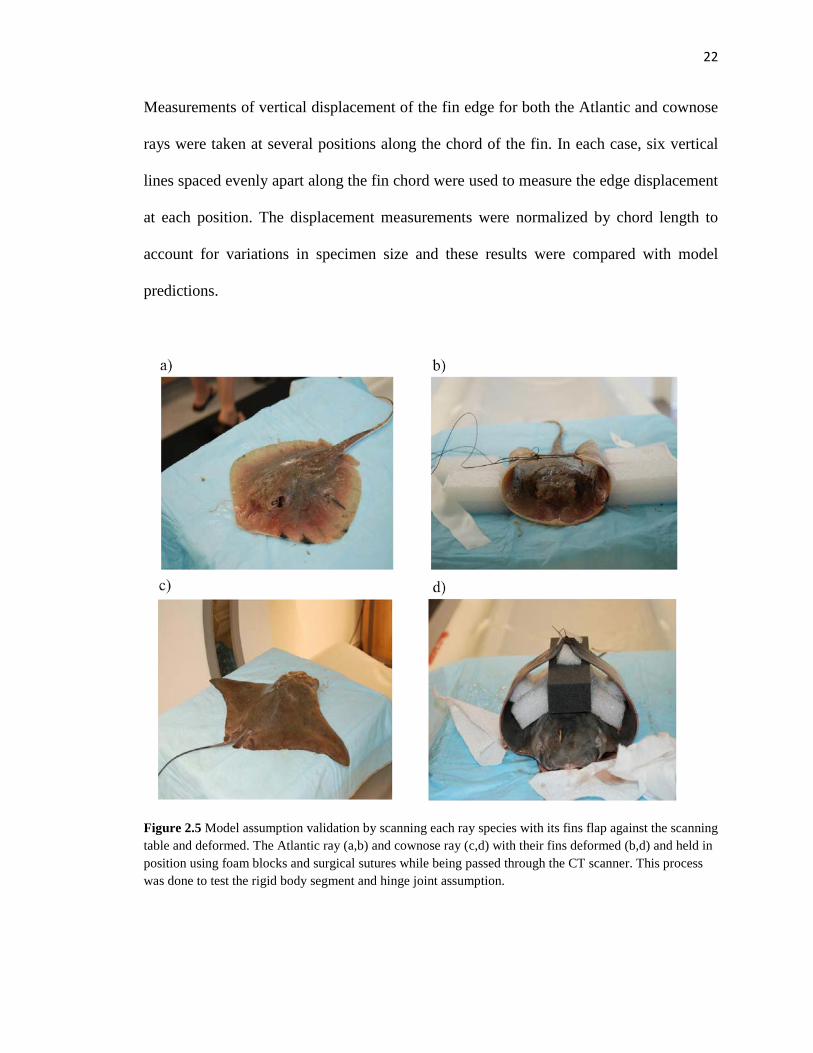
2.1.4 in vivo ray swimming comparison

Video data of ray swimming was collected at West Chester University of

Pennsylvania Liquid Life Laboratory and compared to the model outputs for validation.

(2.8)

20

Figure 2.3 Comparison between the model outputs for the Atlantic ray and in vivo swimming data with qualitative comparisons (a), and quantitative comparisons (b). The motion was tracked in time with three time points reported and displayed as a percentage of the gait cycle.

21

Figure 2.4 Comparison between the model outputs for the cownose ray and in vivo swimming data with qualitative comparisons (a) and quantitative comparisons (b).

22

Measurements of vertical displacement of the fin edge for both the Atlantic and cownose

rays were taken at several positions along the chord of the fin. In each case, six vertical

lines spaced evenly apart along the fin chord were used to measure the edge displacement

at each position. The displacement measurements were normalized by chord length to

account for variations in specimen size and these results were compared with model

predictions.

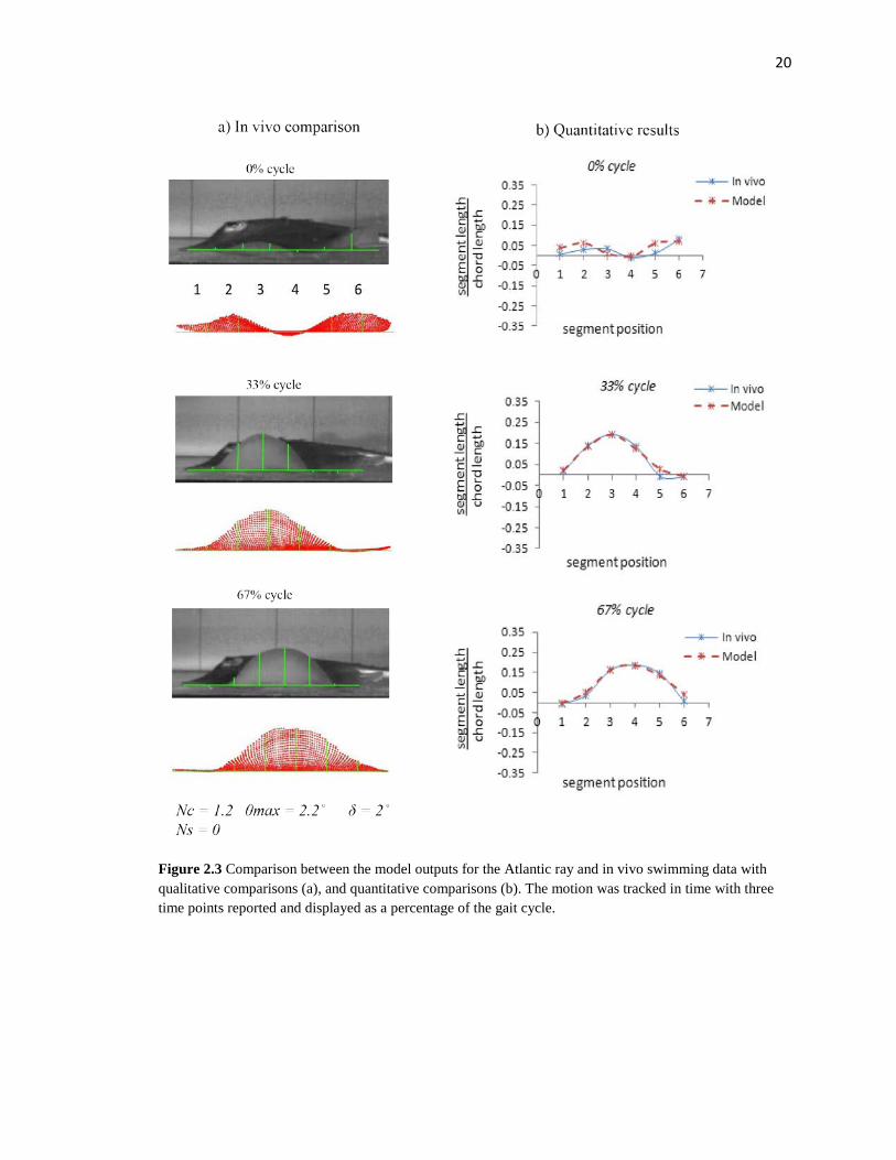
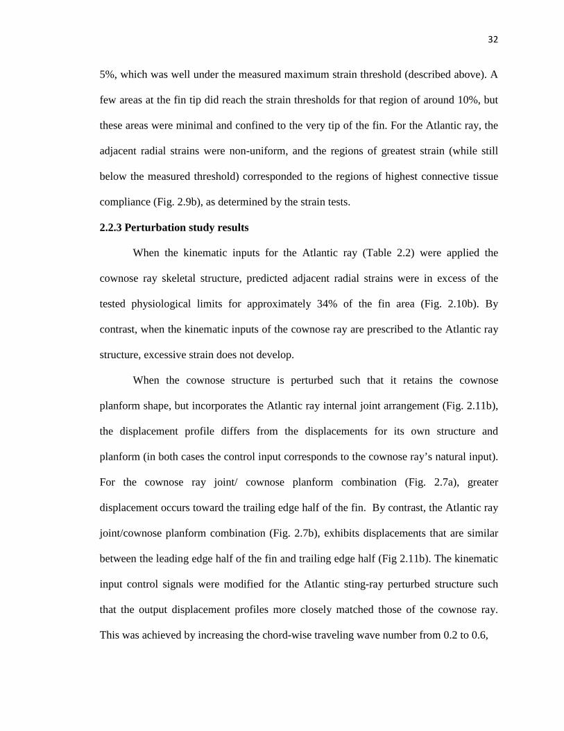
Figure 2.5 Model assumption validation by scanning each ray species with its fins flap against the scanning table and deformed. The Atlantic ray (a,b) and cownose ray (c,d) with their fins deformed (b,d) and held in position using foam blocks and surgical sutures while being passed through the CT scanner. This process was done to test the rigid body segment and hinge joint assumption.

23

The rigid body/hinge joint assumptions were validated via further CT imaging of

the two candidate rays while in a deformed configuration. The fins of each ray were

placed into a position with their fins flexed upward, as seen during oscillatory motion,

and passed through the scanner with the fins held in this position (Fig. 2.5). Each fin was

positioned in a fully flexed state, which corresponded to an apparent non-injurious

physiological limit of the fin. OsiriX Imaging Software was used to digitize the cartilage

structure in both the flat and deformed configurations. To provide a quantitative

assessment of the assumption that segments behave as rigid bodies, a rigid body rotation

analysis was performed for a single radial element that was sectioned out of the CT

reconstructions. The spatial coordinates (xyz) of each cartilage joint were digitized from

the images of the fin when flat and deformed. Using the biomechanical model, deflection

angles were applied to the radial segments (assuming rigid body motion of the segments)

and the results compared to the CT images.

2.1.5 Biomaterial Testing

To determine the implications of the adjacent radial strain calculations, uniaxial

tensile tests were carried out to quantify the failure strain of the adjacent radial

connective tissue. Sections of the underlying cartilage were dissected from cownose rays

(n=4) and Atlantic ray (n=5) fin specimens for mechanical load testing. A 15-gage

scalpel was used to remove the ray skin and muscle from the ray skeleton leaving behind

just the radial elements with adjacent radial connective tissue still intact. The whole

cartilage structure was segmented into samples for testing (Fig. 2.6a). The ends of the

cartilage samples were inserted into clamps that were custom manufactured using a

24

Dimension 1200es Series 3D-printer and were made compatible with an Instron

Microtester (Fig. 2.6a). Tensile loading was applied to the cartilage section in the

direction perpendicular to the long axis of the cartilage segments, resulting in uniaxial

straining of the adjacent radial connective tissue. Extension continued until failure of the

connective tissue was reached as determined by an abrupt drop in load. Load and

displacement measurements were recorded and applied strain to the sample was

measured by tracking the displacement between two reflective tags using a laser

extensometer (Fig. 2.6b) calibrated for a tag displacement range of 0-5mm. Multiple

cartilage samples were extracted from each fin at different locations so that the strain

thresholds throughout the fin could be determined.

Figure 2.6 Samples of cartilage were dissected out of the ray (a) and inserted into a custom testing apparatus (b). Tension was applied in the direction perpendicular to the radial segment’s long axis (a-yellow). Load and displacement measurements were taken with load measured using a built in load cell and displacement measured using a laser extensometer in which a laser beam was used to track distance between two reflective tags. Force and strain data were acquired for analysis (c).

25

The chord length at the fin root of the cownose ray specimens was approximately

42+2cm. Each of the Atlantic ray specimens had a chord length of approximately

20+2cm. The cownose ray specimens, being considerably larger than the Atlantic rays,

provided 10 samples per fin and the Atlantic ray provided 4 samples per fin.

2.1.6 Perturbation Studies

Perturbation studies were carried out to determine the influence of skeletal

morphology on kinematics. To conduct this analysis, kinematic inputs were found for

both the Atlantic and cownose rays performing their respective natural swimming gaits

(Figs. 2.3,2.4). Each set of kinematics was applied to both skeletal structures, where the

skeletal structure of the Atlantic ray was forced to perform motions of the cownose ray

and vice versa. Two perturbation studies involving the skeletal morphology were also

simulated. In perturbation study 1, a cownose ray cartilage structure (Fig. 2.7c) was

compared to an Atlantic sting-ray skeletal structure (Fig. 2.7a) that was artificially altered

such that the overall planform matched that of the cownose ray while preserving the

Atlantic ray's internal cartilage structure (Fig 2.7b). In perturbation 2, the converse was

conducted where an Atlantic ray cartilage structure was compared to the cownose ray

structure that was altered to have the planform of the Atlantic ray (Fig 2.7d). The two

biological structures, cownose ray, and Atlantic sting-ray may also be referred to later in

this text as CR and ASR respectively. For the perturbed structures, the cownose ray

perturbed, and Atlantic sting-ray perturbed structures may also be referred to as CRP and

ASRP respectively. In perturbation study 1, radial segments and joints were added on to

the edge of the naturally occurring Atlantic ray cartilage structure to alter its planform

26

Figure 2.7 Perturbation study structures with the unaltered Atlantic ray structure (a), perturbed to have the same planform as the cownose ray (b), for comparison to the unaltered cownose ray structure (c). The same was done for the converse perturbation study in which the Atlantic ray structure (a) was compared to the cownose ray structure perturbed to have the planform of the Atlantic ray (d).

shape. Radial elements were then removed so that each structure had the same total

number of radial elements, followed by removing every other column of joints so that the

total number of segments running along the span at the mid-chord position was as close

as possible between the two structures. Finally, the artificial structure was scaled in both

chord-wise and span-wise directions so that its span and aspect ratio matched those of the

cownose ray. For perturbation study 2, joints were removed from the cownose ray

27

structure to reduce the planform down to match that of the Atlantic sting-ray. Radial

elements, instead of being removed as in perturbation study 1, were added to the leading

and trailing edge to match the total number of radial elements between the two structures.

This was also necessary to build up the cownose ray structure at the leading and trailing

edge in order to match the Atlantic sting-ray planform.

2.2 Results

2.2.1 Skeletal parameter measurements

Measurements quantifying the skeletal parameter values for the cownose and

Atlantic ray cartilage structures were taken from the digitized CT scans (Fig 2.1). The

results on the IRJP angle, fanning angle, and planform dimensions were recorded and are

provided in table 2.1.

2.2.2 Validation

The kinematics derived from the model for both the Atlantic and cownose rays

compared favorably with the in vivo ray swimming measurements. The error between the

measured displacements and the model predictions was 4.3% for the cownose ray and

8.4% for the Atlantic ray; where percent values are obtained by calculating displacement

error and normalizing by flapping amplitude (Fig. 2.3, 2.4). The parameter inputs

Table 2.1: Skeletal parameter measurements for the cownose and Atlantic ray specimens

28

Morphometrics cownose ray Atlantic ray

R 87 108

S 26 22

Total No. of Joints 1202 1645

Span length 279mm 162mm

Chord length 344mm 343mm

Planform Area 28347 mm2 22991 mm2

Skeletal Parameters

IRJP angle (root/mid/distal) 6°/31°/52° 0°/2°/6°

Fanning angle (fore/mid/aft) 8°/-6°/-74° 104°/2 °/-81°

necessary for the cownose and Atlantic rays (Table 2.2) to give rise to favorable matches

with the in vivo data are consistent with the previous descriptions of each species’

swimming patterns [5,9]. The cownose ray required equal parts span- and chord-wise

traveling wave numbers while no span-wise traveling wave was required for the Atlantic

ray for a good kinematic match. Asymmetric flapping was observed for both species with

approximately a 2:1 ratio of upward flap to downward flap for the cownose ray and

nearly upward flap only for the Atlantic ray.

The CT images of the fins in a deformed configuration confirm the cartilage

segments behave as rigid beams. Qualitatively, the segments were not observed to bend

in order to achieve the necessary span-wise curvature (Fig 2.8a, b, e, f) with deformation

held to rotation at the joints. The quantitative assessment demonstrated that the model,

assuming rigid body motion, provided a high level of agreement with the observed joint

29

motions. The differences between the predictions from the rigid-body model and the

observed displacements were less than 2% for both the cownose ray and the Atlantic ray.

Table 2.2: In vivo kinematic inputs for cownose and Atlantic ray

Kinematic parameter cownose ray Atlantic ray

Amplitude of oscillation (θmax) 1.45° 2.20°

Chord-wise traveling wave number (Nc) 0.2 1.2

Span-wise traveling wave number (Ns) 0.2 0.0

Asymmetric shift (δ) 0.5° 2.0°

2.2.2 Biomaterial strain thresholds

The material testing results revealed how the compliance of the adjacent radial

connective tissue varies throughout the fin, and by species (Fig. 2.9). The average strain

threshold for the cownose ray was 9.89% (standard deviation 2.64%) and 16.52%

(standard deviation 5.01%) for the Atlantic ray, with “threshold” referring to the strain

level where failure occurred. Compliance of the connective tissue of the cownose ray

increased from leading to trailing edges for more proximal regions of the fin. A slight

increase in compliance was also observed toward the most distal regions of the fin (Fig.

2.9a). With an average strain threshold value of 16.52%, the Atlantic ray connective

tissue was nearly twice as compliant as that of the cownose ray. The compliance for the

Atlantic ray also differed by region, where the most significant increases in compliance

30

Figure 2.8 Single radial elements sectioned out of the reconstructed CT images of the Cownose ray (a,b) and Atlantic ray (e,f) with virtual representations of the radial element from the flat fin (blue) and the in situ deformed fin (maroon). Both cases for each species were plotted against one another (c,g). Rigid body rotation was then applied to the radial segments of the flat radial element such that the radial element from the flat case matched the curvature of the radial element of the deformed case (d,h).

was located near the distal trailing edge, where a strain threshold of 24% was measured

(Fig 2.9b). The results of this testing proved important for interpreting the modeling

results as they provided values of acceptable strain level. The strain thresholds were also

used to determine the kinematic limits of a given skeletal structure which allowed for the

range of motion of a given skeletal structure to be defined.

2.2.3 Biomaterial strain thresholds

When each of the ray’s kinematic inputs were applied to its corresponding

skeletal structure, the displacement and strain profiles clearly differed between the two

31

Figure 2.9 Results of material tests of the adjacent radial connective tissue with strain thresholds reported in accordance with position throughout the fin. Tests were performed on 4 cownose ray fins at 10 locations (a) and on 5 Atlantic ray fins at 4 locations (b). Samples were taken from the shaded yellow regions with specific areas indicated by numbers which correspond to the bar graphs.

species as expected (Fig. 2.10). For the cownose ray, the adjacent radial strains were

relatively uniform, where the majority of peak adjacent radial strain levels were less than

32

5%, which was well under the measured maximum strain threshold (described above). A

few areas at the fin tip did reach the strain thresholds for that region of around 10%, but

these areas were minimal and confined to the very tip of the fin. For the Atlantic ray, the

adjacent radial strains were non-uniform, and the regions of greatest strain (while still

below the measured threshold) corresponded to the regions of highest connective tissue

compliance (Fig. 2.9b), as determined by the strain tests.

2.2.3 Perturbation study results

When the kinematic inputs for the Atlantic ray (Table 2.2) were applied the

cownose ray skeletal structure, predicted adjacent radial strains were in excess of the

tested physiological limits for approximately 34% of the fin area (Fig. 2.10b). By

contrast, when the kinematic inputs of the cownose ray are prescribed to the Atlantic ray

structure, excessive strain does not develop.

When the cownose structure is perturbed such that it retains the cownose

planform shape, but incorporates the Atlantic ray internal joint arrangement (Fig. 2.11b),

the displacement profile differs from the displacements for its own structure and

planform (in both cases the control input corresponds to the cownose ray’s natural input).

For the cownose ray joint/ cownose planform combination (Fig. 2.7a), greater

displacement occurs toward the trailing edge half of the fin. By contrast, the Atlantic ray

joint/cownose planform combination (Fig. 2.7b), exhibits displacements that are similar

between the leading edge half of the fin and trailing edge half (Fig 2.11b). The kinematic

input control signals were modified for the Atlantic sting-ray perturbed structure such

that the output displacement profiles more closely matched those of the cownose ray.

This was achieved by increasing the chord-wise traveling wave number from 0.2 to 0.6,

33

Figure 2.10 Motion simulations for each structure performing the motions of one another. Kinematic inputs for the Atlantic ray were applied to both structures with qualitative outputs from the model (a), and associated adjacent radial strain distribution (b). The same was repeated for the kinematic inputs for the cownose ray with qualitative outputs (c), and strain distributions (d).

34

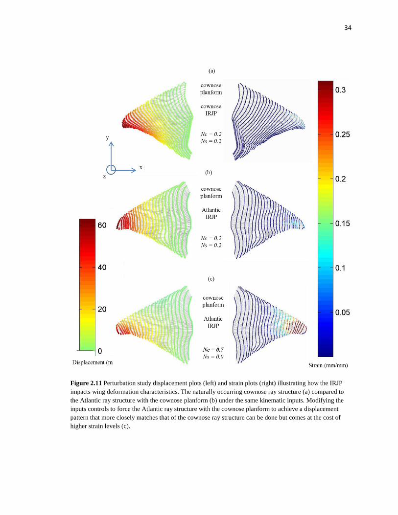
Figure 2.11 Perturbation study displacement plots (left) and strain plots (right) illustrating how the IRJP impacts wing deformation characteristics. The naturally occurring cownose ray structure (a) compared to the Atlantic ray structure with the cownose planform (b) under the same kinematic inputs. Modifying the inputs controls to force the Atlantic ray structure with the cownose planform to achieve a displacement pattern that more closely matches that of the cownose ray structure can be done but comes at the cost of higher strain levels (c).

35

and decreasing the span-wise traveling wave number to 0.0 (Fig. 2.11c). However in this

scenario, the resulting excessive adjacent radial strains were far greater than the

experimentally determined threshold limits found in the tension experiments.

Figure 2.12 Perturbation study 2 displacement plots (left) and strain plots (right). The Atlantic ray structure (a) was compared to the cownose ray structure with the Atlantic planform (b) under the same kinematic inputs. The fin structure was plotted in the non-deformed state to aid in the proper visual representation of the strain distribution. This was not done for the displacement plots which explain the differences in the outline appearance between the fins.

The Atlantic ray structure (Fig 2.12a) was compared to the cownose ray structure

with the Atlantic ray planform (i.e., cownose ray perturbed) (Fig 2.12b). A similar trend

observed in perturbation study 1, where the skeletal patterns of the cownose ray direct

more of the joint displacement toward the trailing edge, seemed to occur for perturbation

study 2 also. The strains observed were slightly higher for the Atlantic ray structure but

36

both fins strain levels were within the tested threshold with the exception of a few areas

toward the outer fin edges.

2.3 Discussion

The biomechanical model presented in this study couples a given ray cartilage

structure with prescribed kinematics, and is shown to be capable of accurately

reproducing the natural motions observed for the cownose and Atlantic rays. It was

demonstrated how the skeletal structure of real rays would have to function in order to

accommodate swimming gaits. It was also show that the model helps provide an

explanation of the link between the internal cartilage patterns in rays and the kinematics

associated with these patterns. The predictions of the adjacent radial strain required to

accommodate certain motions provided insight into the physical limits of a given fin

structure. The biomaterial testing further allowed for the model’s strain predictions to be

better interpreted, and for kinematic limits of a given fin structure to be known.

The modeling results for skeletal perturbation study 1(Fig. 2.11), show that both

skeletal structure and planform shape affect fin kinematics. The modeling results

demonstrated that the internal cartilage arrangement is important, and that it has an effect

on the strain-displacement relationship of the fin structure (Fig 2.11, 2.12). The skeletal

perturbation studies revealed that the inter-radial joint pattern (IRJP) impacts deformation

characteristics of the fin, and that this pattern can be a mechanism for altering fin flexion

properties without requiring changes in planform or higher levels of adjacent radial strain

(Fig. 2.11). A more angled IRJP, where the pattern converges toward the tail (Figure

37

2.11a), seems to direct the fin flexion towards the trailing edge. Conversely, the Atlantic

ray perturbed structure curls up about an axis that is parallel to the direction of the IRJP.

These results show how altering the internal joint patterns can be an effective method of

achieving some desired fin displacement. Prior research on the effects of this pattern [18]

agrees with this concept; however analyses involving in situ skeletal morphometry were

not conducted, nor were adjacent radial strain levels considered. The kinematic effects of

variations in the internal cartilage arrangement will most likely have an impact on the

hydrodynamic performance. To explore this hypothesis, it was necessary to incorporate a

fluid mechanics model into the study, and Chapter 3 explains how this was done to

establish a link between skeletal design and swimming performance.

Understanding the implications of the predicted strain levels is important when

analyzing the kinematic potential of a given fin structure. The strain analysis of the

motion perturbation study (Fig. 2.10) illustrate that the cownose ray develops adjacent

radial strain levels in excess of the physiological limits if forced to perform the

undulatory motions of the Atlantic ray (see Fig. 2.9). This kinematic pattern implies that

this motion would not be feasible for a cownose ray, and such undulatory gaits could

therefore not be achieved. Furthermore, strain distribution plots of the Atlantic ray

performing its intended natural motion (Fig. 2.10b – left), when compared to the tested

strain thresholds (Fig. 2.9b), shows that the highest strain levels correspond to the area of

greatest compliance in the Atlantic ray fin (Fig. 2.9b). These results suggest that Atlantic

ray may have evolved to accommodate this strain requirement by increasing the

compliance and failure strain limits of the connective tissue in select regions.

38

Perturbation study 1 (Fig 2.11), demonstrated that for the perturbed ASRP structure, a

displacement profile that matches that of the cownose ray can be achieved through

manipulating the input kinematics (Fig. 2.11c – left). However, this comes at the expense

of higher levels of adjacent radial strain (Fig. 2.11c – right). This sets up the hypothesis

that the skeletal structure of the cownose ray can achieve a kinematic profile that may

carry performance advantages without requiring high strain levels.

Although many insights can be gained from modeling the kinematics of the

underlying skeletal structure, there are many other factors at play with regard to the

whole pectoral fin system that cannot be explained with the model introduced in this

study. The model shows that skeletal morphology impacts kinematics. To understand

how kinematic variations, as a result of skeletal variations, affect swimming performance,

it was necessary to incorporate a computational fluid dynamics (CFD) component. In the

following chapter, a method for coupling the biomechanical model with CFD is

introduced which allowed for the motion and morphology perturbation studies to be

revisited from a hydrodynamics perspective, where metrics such as thrust production,

propulsive efficiency, swimming speed, and cruising economy can be used to quantify

the effect of skeletal design on the hydrodynamic performance.

Prior studies have shown that undulation and oscillation are correlated with very

different swimming performance characteristics [7,8,11] and body shapes [5,8,17], which

can be incorporated into the design of an artificial fin. Techniques for simulating the

motion of a fin, from both internal and external perspectives [27,55] have been explored,

but none have shown how the actual biological structure can function mechanically to

create this motion. Through this approach, the skeletal designs observed in nature can be

39

explained and, where appropriate, applied to the mechanical design of artificial systems.

The results of the skeletal perturbation studies (Fig. 2.11, 2.12) show that the input

kinematics (e.g., Nc, Ns, θmax) and the internal cartilage arrangement are both

mechanisms for determining ray locomotion. The results regarding the strain-

displacement relationship as a function of internal cartilage arrangement can be used to

inform the placement of the nodes of artificial structures, such as those proposed by other

researchers [12,15,36], to assist in achieving desired fin kinematics while keeping strain

levels to a minimum. In such applications the biomechanical model can be used to

determine where high levels of compliance may be needed in an artificial fin or how

rearrangement of the structure nodes can induce kinematic change without leading to an

increase in fin strain or compliance requirement. To further explain and understand these

concepts, the effects of the skeletal design parameters (i.e., IRJP angle and fanning angle)

on system performance (i.e., kinematics and hydrodynamics) are quantified

independently through the parameterized modeling studies discussed in chapter 4, and the

follow on experimental work discussed in chapter 5 explores how the biomechanical

model can be used to drive the design of artificial fins.

40

Chapter 3

Fluid-Structure-Interaction (FSI) modeling

A method for interfacing the biomechanical model with a CFD model is

introduced, and the perturbation studies are revisited from a hydrodynamics perspective.

In Chapter 2, it was shown that the internal cartilage arrangement influences fin

kinematics regardless of planform shape. In this chapter, the relationship between skeletal

design and hydrodynamic performance is explored through the integration of a

biomechanical model of ray musculoskeletal systems with an advanced panel method,

free-swimming, CFD model. The effect of skeletal variations on fin kinematics and

propulsion is explored through the skeletal perturbation studies discussed in chapter 2.

With the CFD coupling in place, the link between skeletal design and hydrodynamic

performance can be established. Performance metrics including thrust production,

propulsive efficiency, steady-state swimming speed, and cruising economy are calculated

for both normal and perturbed skeletal structures.

The specific objectives for this chapter were to 1) develop a method for

interfacing the biomechanical model with an advanced panel method CFD mode, 2)

expand the perturbation studies of chapter 2 to include hydrodynamics in order

complete the loop between skeletal design, kinematics, and propulsion, and 3)

identify potential aspects of the biological systems that could be leveraged in the

design of artificial pectoral fin systems for use in AUVs. The fluid structure modeling

results show that particular patterns in the skeletal structure can enable preferential fin

41

deformation characteristics, leading to increased low speed thrust production and greater

propulsive efficiency over a range of stream-wise swimming velocities. Results also

showed that particular skeletal designs may be necessary to achieve efficient swimming

gaits without requiring excessive structural strain between skeletal elements. The

importance of swimming gait selection for efficient acceleration and cruising was also

analyzed.

3.1 Materials and Methods

3.1.1 Unsteady Panel Method

Since batoid rays swim using unsteady hydrodynamics, an unsteady CFD model

must be used. A previously developed panel method and code [52], in which a series of

rectangular panels are connected to form a three dimensional body, was adopted in this

research to simulate interaction with a fluid environment. Discretization of the ray fin,

body and associated wake structure is used compute the forces acting on the fin and body

and works for both free-swimming and fixed velocity cases. The method works by

implementing the unsteady Bernoulli equation for solving for the pressure solution over

each panel. Since this is solved for each panel separately, as opposed to solving for the

entire flow field (i.e., near and off body), the method is computationally efficient.

Additionally, the panel method incorporates a viscous drag correction for improved

accuracy can also model the free-wake structure that contributes to the forces acting on

the body. The computational speed, wake formation modeling capability, and

42

incorporation of viscous drag make the panel method ideal for application to the present

research by allowing for fast yet detailed analysis of the hydrodynamics.

3.1.2 Joint displacement to panel node displacement mapping

The panel method depends on a set of known panel kinematics in order to

function. To establish an interface between the biomechanical model and panel method

CFD model, a technique for transforming the biomechanical model kinematics to panel

kinematics was needed. To solve this problem, a method for mapping time varying

displacement of skeletal joints was developed. This resulted in a system in which the

motion of the underlying skeletal structure was used to drive the motion of an overlaying

three dimensional body composed from a series of connected panels.

A shape function interpolation method was used in which a two-dimensional

mesh of triangular elements was used to represent the skeletal structure. In this

application, the element nodes were the same as the skeletal joint positions, which

amounted to a system in which the triangular element node displacements were solved

concomitantly with skeletal joint displacement. To begin solving for panel node

positions, an array or grid points is generated and overlain on the fin cartilage structure.

Each panel corner point contained within the fin area will fall into one of the triangular

elements (see Fig 3.1). Since the biomechanical model has already been used to define

the displacements of every joint at each time step, then the displacement of the each

triangular element is also known, as joint positions double as element nodes. The relative

43

displacements between the nodes of each element were therefore used to solve for the

corresponding displacement of each panel corner point from the equation:

𝑸𝑖𝑗(𝑡) = 𝜦𝑖𝑗𝑚�̂�𝑥 ∙ 𝑁𝑚(𝑡)�̂�𝑥 + 𝜦𝑖𝑗𝑚�̂�𝑦 ∙ 𝑁𝑚(𝑡)�̂�𝑦 + 𝜦𝑖𝑗𝑚�̂�𝑧 ∙ 𝑁𝑚(𝑡)�̂�𝑧

where 𝑁𝑚(𝑡) is a (3x3) matrix whose columns are the position vectors of each node of

triangular element m that contains panel corner point 𝑷𝑖𝑗, and the matrix 𝜦𝑖𝑗𝑚 contains

row vector representations of the barycentric coordinates of panel corner point 𝑷𝑖𝑗 , with

respect to the nodes of element m, and since the joint positions double as the element

node positions such that:

𝑁𝑚(𝑡)�̂�𝑥 = 𝒖1𝒎(𝑡)

𝑁𝑚(𝑡)�̂�𝑦 = 𝒖2𝒎(𝑡)

𝑁𝑚(𝑡)�̂�𝑧 = 𝒖3𝒎(𝑡)

where 𝒖1𝒎(𝑡), 𝒖2𝒎(𝑡), 𝒖3m(𝑡) ∈ 𝑼𝑟𝑠(𝑡), and are vectors defining the cartilage joint

displacements that correspond to the nodes of elements m, required for solving the time

varying displacement field 𝑸𝑖𝑗(𝑡) that defines panel kinematics.

(3.1)

(3.2)

(3.3)

(3.4)

44

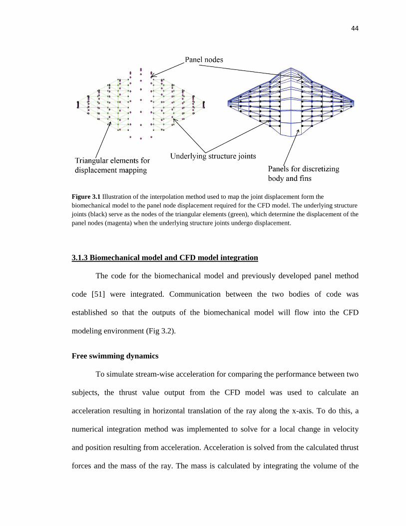
Figure 3.1 Illustration of the interpolation method used to map the joint displacement form the biomechanical model to the panel node displacement required for the CFD model. The underlying structure joints (black) serve as the nodes of the triangular elements (green), which determine the displacement of the panel nodes (magenta) when the underlying structure joints undergo displacement.

3.1.3 Biomechanical model and CFD model integration

The code for the biomechanical model and previously developed panel method

code [51] were integrated. Communication between the two bodies of code was

established so that the outputs of the biomechanical model will flow into the CFD

modeling environment (Fig 3.2).

Free swimming dynamics

To simulate stream-wise acceleration for comparing the performance between two

subjects, the thrust value output from the CFD model was used to calculate an

acceleration resulting in horizontal translation of the ray along the x-axis. To do this, a

numerical integration method was implemented to solve for a local change in velocity

and position resulting from acceleration. Acceleration is solved from the calculated thrust

forces and the mass of the ray. The mass is calculated by integrating the volume of the

45

body and fin regions and multiplying by body density, where density was assumed to be

equal to that of water.

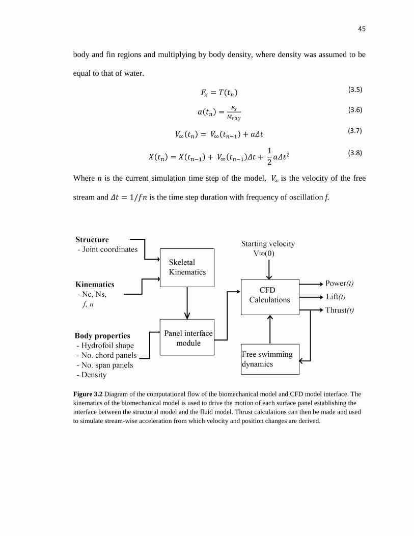
𝐹𝑥 = 𝑇(𝑡𝑛)

𝑎(𝑡𝑛) = 𝐹𝑥𝑀𝑟𝑎𝑦

𝑉∞(𝑡𝑛) = 𝑉∞(𝑡𝑛−1) + 𝑎𝛥𝑡

𝑋(𝑡𝑛) = 𝑋(𝑡𝑛−1) + 𝑉∞(𝑡𝑛−1)𝛥𝑡 + 12𝑎𝛥𝑡2

Where n is the current simulation time step of the model, 𝑉∞ is the velocity of the free

stream and 𝛥𝑡 = 1/𝑓𝑛 is the time step duration with frequency of oscillation f.

Figure 3.2 Diagram of the computational flow of the biomechanical model and CFD model interface. The kinematics of the biomechanical model is used to drive the motion of each surface panel establishing the interface between the structural model and the fluid model. Thrust calculations can then be made and used to simulate stream-wise acceleration from which velocity and position changes are derived.

(3.5)

(3.6)

(3.7)

(3.8)

46

3.1.4 Hydrodynamic performance metrics

Simulation results were analyzed by comparing the thrust production, propulsive

efficiency, cruising speed, and cruising economy for each of the four structures. Each

simulation was initiated at a stream-wise flow velocity of near zero to approximate

acceleration from rest. The simulation was continued for 10 cycles for each structure,

which allowed sufficient time for the body to accelerate from rest to a steady-state

velocity. Thrust production and propulsive efficiency was analyzed for the transient

period in which acceleration is present. Thrust and efficiency quantities were computed

across increasing velocities during the acceleration period. This allowed for the thrust

generating capacity, and efficiency in doing so, to be compared between multiple

structures at various velocities. Thrust, hydrodynamic power, and velocity values were

sampled at each time step and reported values for thrust, velocity, and efficiency were

obtained by computing the average values across every half-cycle during a 10 cycle

simulation. This was done along the entire acceleration period until steady-state velocity

was reached; at which point the cycle averaged thrust production is zero. Reported thrust,

propulsive efficiency, and stream-wise velocity were computed by numerical integration

as follows:

𝑇𝑎𝑣𝑔(𝑐𝑦𝑐𝑙𝑒0.5) = 2𝑁𝑠𝑡𝑒𝑝

∙ ∑ 𝑇(𝑡𝑛)𝑖+ 𝑁𝑠𝑡𝑒𝑝

2 𝑛= 𝑖

𝑉𝑎𝑣𝑔(𝑐𝑦𝑐𝑙𝑒0.5) = 2𝑁𝑠𝑡𝑒𝑝

∙ ∑ 𝑉∞(𝑡𝑛)𝑖+ 𝑁𝑠𝑡𝑒𝑝

2 𝑛= 𝑖

𝑃𝑎𝑣𝑔(𝑐𝑦𝑐𝑙𝑒0.5) = 2𝑁𝑠𝑡𝑒𝑝

∙ ∑ 𝑃(𝑡𝑛)𝑖+ 𝑁𝑠𝑡𝑒𝑝

2 𝑛= 𝑖

(3.9)

(3.10)

(3.11)

47

𝜂𝑝(𝑐𝑦𝑐𝑙𝑒0.5) = 𝑇𝑎𝑣𝑔

(𝑐𝑦𝑐𝑙𝑒0.5)∙ 𝑉𝑎𝑣𝑔(𝑐𝑦𝑐𝑙𝑒0.5)𝑃𝑎𝑣𝑔(𝑐𝑦𝑐𝑙𝑒0.5)

where, 𝑖 = 12𝑁𝑠𝑡𝑒𝑝( 𝑐𝑦𝑐𝑙𝑒0.5 − 1) + 1 , 𝑐𝑦𝑐𝑙𝑒0.5 denotes the half-cycle being integrated,

and 𝑁𝑠𝑡𝑒𝑝 is the total number of time steps per cycle. Since the cycle averaged thrust

production decays to zero once steady-state velocity is reached, the propulsive efficiency,

being the product of thrust and velocity, also decays to zero. Therefore at steady-state

swimming, the propulsive efficiency of the whole system, calculated as the ratio of the

propulsive power to overall power, is also zero and no longer a meaningful metric. In

order to analyze the performance of swimming at steady-state (i.e., cruising), a different

metric was used, steady-state economy. The steady-state economy is defined as the unit

of distance traveled per unit of energy expended. In this case, economy is expressed in

units of body lengths (BL) per Joule. This is equivalent to the familiar metric of miles per

gallon used in the automobile industry, and was used to compare cruising performance

between different fin designs. Economy was calculated from the cycle-averaged power

and cycle-averaged velocity as follows:

𝐸𝑠𝑠 = 𝑉𝑠𝑠𝑃𝑠𝑠

where 𝑉𝑠𝑠 = 1𝑁𝑠𝑡𝑒𝑝 ∆𝑡

∙ ∫ 𝑉∞(𝑡)𝑑𝑡, and 𝑃𝑠𝑠 = 1𝑁𝑠𝑡𝑒𝑝 ∆𝑡

∙ ∫ 𝑃(𝑡)𝑑𝑡, and is evaluated

over the last cycle after steady-state velocity has been reached.

(3.12)

(3.13)

48

3.1.5 Perturbation studies (Hydrodynamics)

Hydrodynamic simulations were run for the four skeletal structures involved in

the perturbation studies. Both the oscillating structures of perturbation study 1, and

undulating structures of perturbation study 2, were revisited from a hydrodynamic

perspective. Simulations were run with the in vivo observed kinematics prescribed and

the resulting performance was compared. To further explore the parameter space,

kinematics was prescribed for a range of chord- and span-wise traveling wave numbers

(Nc & Ns) near those for the in vivo matched cases. This was done to examine the effect

of gait control on performance as it is feasible that rays have the ability to modify their

swimming gait to maintain good performance as conditions vary.

Perturbation study 1

The cownose ray structure (Fig 2.7c) was compared to the Atlantic ray structure

that was perturbed to have the same planform as the cownose ray (Fig 2.7b). Simulations

were run for each structure over a range of kinematic parameters, including the in vivo

case of chord- and span-wise traveling wave numbers of 0.2 waves (i.e., Nc=0.2, Ns=0.2,

see Fig 2.4). The full test matrix for perturbation study 1 is provided in Table 3.1.

Perturbation study 2 – hydrodynamic simulations

Conversely, the Atlantic ray structure (Fig 2.7a) was compared to the cownose ray

structure that was perturbed to have the same planform as the Atlatnic ray (Fig 2.7d).

Simulations were run for each structure over a range of kinematic parameters, including

49

the in vivo case of a chord-wise traveling wave number of 1.2 waves (i.e., Nc = 1.2, Ns =

0.0, see Fig 2.3). Since the video analysis discussed in Chapter 2 showed that the addition

of a span-wise traveling wave was not needed for a kinematic match in this case, only

motions involving chord-wise traveling waves were simulated for perturbation study 2.

The full test matrix for perturbation study 2 is provided in Table 3.2.

Table 3.1: Test matrix for perturbation study 1 (Hydrodynamics)

Kinematic parameter Test Range

Nc, chord-wise traveling wave number 0.0 – 0.4 by increments of 0.2

Ns, span-wise traveling wave number 0.0 – 0.4 by increments of 0.2

f, frequency of oscillation 1 Hz

Table 3.2: Test matrix for perturbation study 2 (Hydrodynamics)

Kinematic parameter Test Range

Nc, chord-wise traveling wave number 0.8 – 1.2 by increments of 0.2

Ns, span-wise traveling wave number 0.0

f, frequency of oscillation 1 Hz

For both perturbation studies, the amplitude was set to the peak-to-peak amplitude

that was recorded from the in vivo video analysis, which corresponded to the fin tip

flapping amplitude equal to approximately 50% of the span length. The frequency of 1Hz

was selected because it falls in the middle of the range of swimming frequencies

previously reported for both the cownose and Atlantic ray [4, 5]. As the primary focus of

50

this work was to examine the effects of skeletal design on performance, the frequency

and amplitude were held constant to keep the motion parameter space from

overshadowing the skeletal parameter space.

3.2 Results – (perturbation study hydrodynamics)

3.2.1 Perturbation study 1 & 2 results for in vivo prescribed motions

Comparisons between the two oscillating structures and two undulating structures

were made first for the in vivo prescribed motions discussion in Chapter 2 (see Fig 2.3,

2.4), as these cases were of special interest since the kinematic inputs were obtained

directly from biology. Free-swimming simulations were run and comparisons in thrust

production, propulsive efficiency, cruising speed and economy are presented in Fig.3.3.

As shown in Fig. 3.3, the oscillating structures have much higher thrust production and

top speed than the undulating structures. For the non-perturbed “natural” structures, the

cownose ray (CR) produces up to 11.7 times more thrust, and is 1.7 times more efficient

than the Atlantic sting-ray (ASR) when comparing their respective maximum thrust and

efficiency values. At steady state, the cownose ray achieves a cruising speed of 1.36

BL/sec, which is 2.6 times faster than the Atlantic ray’s cruising speed of 0.52 BL/sec.

The Atlantic ray, however, cruises at 0.52 BL/sec with an economy of 411.86 BL/Joule,

which is 7.4 times that of the cownose ray cruising economy of 54.96 BL/Joule (keeping

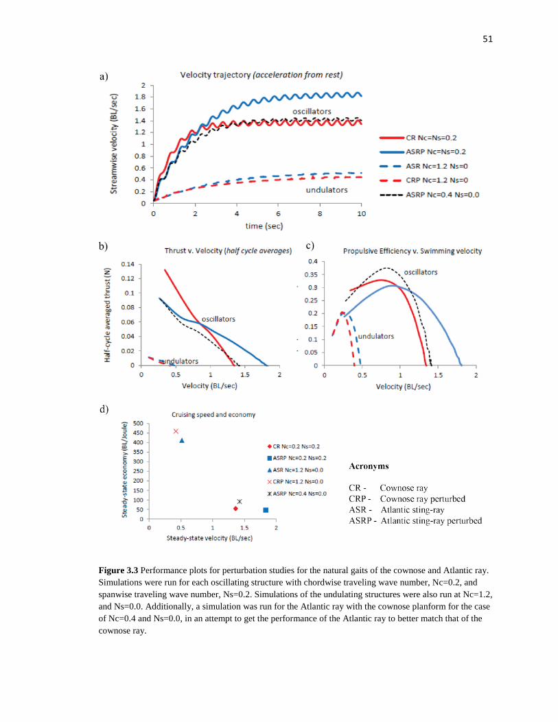
51

Figure 3.3 Performance plots for perturbation studies for the natural gaits of the cownose and Atlantic ray. Simulations were run for each oscillating structure with chordwise traveling wave number, Nc=0.2, and spanwise traveling wave number, Ns=0.2. Simulations of the undulating structures were also run at Nc=1.2, and Ns=0.0. Additionally, a simulation was run for the Atlantic ray with the cownose planform for the case of Nc=0.4 and Ns=0.0, in an attempt to get the performance of the Atlantic ray to better match that of the cownose ray.

52

in mind the small scale of the ray’s being simulated when comprehending the magnitude

of the economy values).

When comparing between the oscillating structures only, the cownose ray

structure produces much greater thrust with higher efficiency levels than the ASRP

structure for velocities at or below 0.8 BL/sec. At the lower velocities, the cownose ray

produces up to 42% more thrust, and is up to 35% more efficient than the Atlantic sting-

ray perturbed. However, the ASRP thrust production overtakes that of the cownose ray at

approximately 0.8 BL/sec, and maintains greater thrust production to achieve a steady

state velocity that is 24.1% faster than the cownose ray. The ASRP structure eventually

achieves a cruising speed of 1.84 BL/sec, compared to the cownose ray’s cruising speed

of 1.36 BL/sec. The cruising economy of the perturbed Atlantic ray was 47.46 BL/Joule,

which is 13.7% less than the cownose ray’s cruising economy of 54.96 BL/Joule, but the

perturbed Atlantic ray is swimming 26.1% faster. Thrust values for the undulating

structures were nearly the same for the in vivo case at the lower velocities, with the

Atlantic ray maintaining slightly higher thrust levels as velocity increased to eventually

achieve a cruising speed of 0.52 BL/sec compared to .42 BL/sec for the cownose ray

perturbed (CRP). The cruising economy of 411.86 BL/Joule for the Atlantic ray was less

than that of the cownose ray perturbed structure of 459.54 BL/Joule, a 10.4% difference,

and similar to the difference calculated between the oscillating structures.

To further understand why differences in performance are observed for structures

that have the same planform shape, but different underlying cartilage patterns, plots of

the source of thrust throughout the fin were generated for both perturbation studies. In

Fig. 3.4, the distribution of thrust forces shown at two critical points for both the cownose

53

ray (CR) and Atlantic sting-ray perturbed (ASRP) (Fig 3.4a). At the point of initial

acceleration (time point 1), both structures show thrust contribution from leading edge

suction, but the cownose ray is getting additional thrust contribution from the trailing

edge which is absent from the Atlantic sting-ray perturbed (Fig 3.4b,d). However, at the

point at which the velocity of the Atlantic sting-ray perturbed structure overtakes that of

the cownose ray (time point 2), we can see that the leading edge suction is less for the

cownose ray, and also added drag has been induced at the trailing edge, which was absent

at the lower velocity (Fig 3.4c,e). The additional thrust contribution from the cownose ray

results in higher overall thrust for the lower velocities, but also causes added drag at

higher velocities suggesting that the very aspect of the system that is leading to improved

performance at the lower speeds is the same thing that is degrading the performance at

the higher speeds.

A similar trend is observed for the Atlantic sting-ray compared the cownose ray

perturbed (Fig 3.5), but the difference in low speed thrust production is not present as it

was in perturbation study 1. It is interesting that the although the total net thrust

production is almost equal for the ASR and CRP structures at the lower speeds, there are

regions of higher thrust production for the CRP structure. However, there are also regions

of higher drag for the CRP structure which seems to counteract the regions of higher

thrust.

In Chapter 2, the joint displacement fields were plotted for each perturbation

study showing differences in joint displacement patterns for similar strain levels,

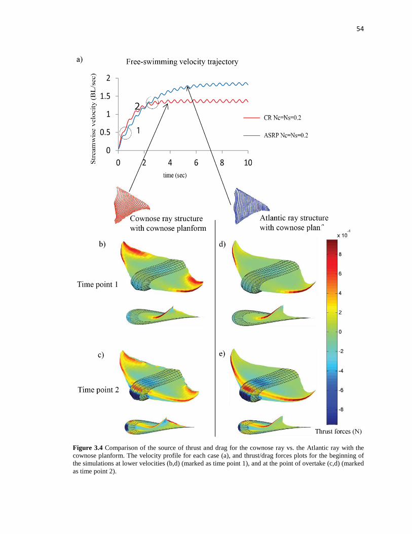
54

Figure 3.4 Comparison of the source of thrust and drag for the cownose ray vs. the Atlantic ray with the cownose planform. The velocity profile for each case (a), and thrust/drag forces plots for the beginning of the simulations at lower velocities (b,d) (marked as time point 1), and at the point of overtake (c,d) (marked as time point 2).

55

Figure 3.5 Comparison of the source of thrust and drag for the Atlantic ray vs. the cownose ray with the Atlantic ray planform. The velocity profile for each case (a), and thrust/drag forces plots for the beginning of the simulations at lower velocities (b,d) (marked as time point 1), and at the point of overtake (c,d) (marked as time point 2).

56

revealing that the joint pattern can be arranged in such a way to change the deformation

of the fin without inducing additional adjacent radial strain levels (see Fig 2.11, and Fig

2.12). It is the airfoil shape, however, and the way it changes with fin position and time

that matters in determining swimming performance. Therefore, quantifying how

differences in joint displacement patterns translate to differences in airfoil kinematics is

important. To connect joint displacement with airfoil kinematics,, the leading edge (LE)

and trailing edge (TE) pitch angles of the fin were calculated at different throughout the

gait cycle. The pitch angle is measured relative to the horizontal at the leading edge point

to the thickest part of the airfoil for the LE calculations, and from approximately two-

thirds the chord-span to the trialing cusp for the TE calculations (Fig 3.6b); LE and TE

pitch angles are calculated from:

𝑝𝐿𝐸𝑗(𝑡) = 90 − cos−1 � [𝑷𝑡_𝑚𝑎𝑥,𝑗(𝑡)− 𝑷1,𝑗(𝑡)]∙�̂�𝑧) �𝑷𝑡_𝑚𝑎𝑥,𝑗(𝑡)− 𝑷1,𝑗(𝑡)�‖�̂�𝑧‖

�

𝑝𝑇𝐸𝑗(𝑡) = 90 − cos−1 �[𝑷𝑐_𝑚𝑎𝑥,𝑗(𝑡)− 𝑷2

3𝑐_𝑚𝑎𝑥,𝑗(𝑡)]∙�̂�𝑧

�𝑷𝑐_𝑚𝑎𝑥,𝑗(𝑡)− 𝑷23𝑐_𝑚𝑎𝑥,𝑗

(𝑡)�‖�̂�𝑧‖�

where t_max and c_max denote the chord position where maximum thickness occurs and

where the trailing edge cusp occurs, respectively. For the present case, t_max = 7, and

c_max = 32, since the maximum chord thickness occurs at a chord-wise panel node

position of 7 when 32 chord-wise panels are used.

Figure 3.6 demonstrates the process of connecting joint kinematics with airfoil

kinematics, and shows the LE and TE pitch angles throughout the gait cycle (Fig 3.6c,d)

for both middle and distal span positions (Fig 3.6a). This analysis offers a kinematic

(3.14)

(3.15)

57

Figure 3.6 Kinematic explanation for the hydrodynamic performance differences between t he cownose ray and perturbed Atlantic ray. Recap of results on the joints displacements from previous studies (a), with 3D visualization of how the joint displacement variations translate into changes in airfoil shape (b). Quantitative data on the time varying leading (c) and trailing (d) edge pitch angles are also reported, showing the greatest difference being at the distal trailing edge.

explanation for the observed differences in hydrodynamic performance. As shown in

figure 3.6c, the maximum pitch angle is slightly higher for the cownose ray for leading

edge. However, a much higher pitch angle of 28.87 degrees is achieved at the trailing

edge of the cownose ray, as compared to 9.22 degrees for the ASRP structure (Fig 3.6d)

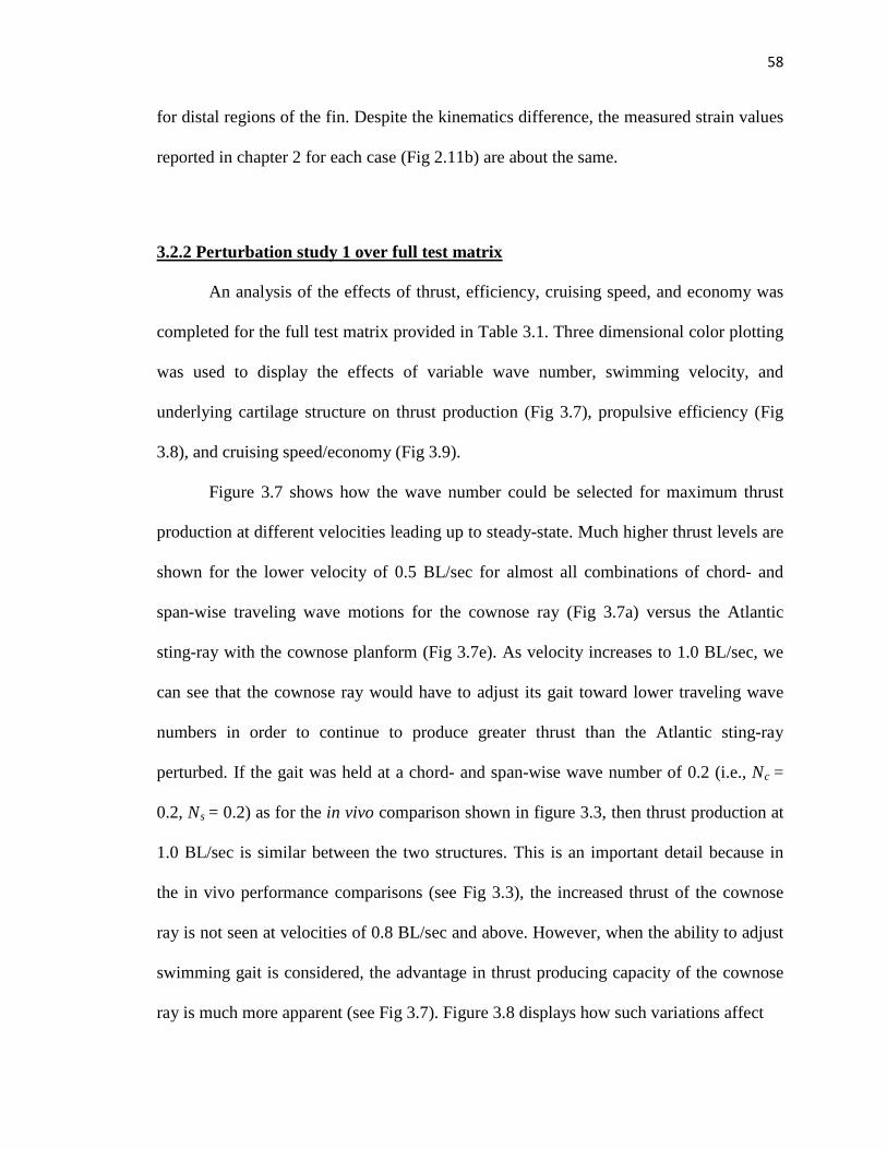
58

for distal regions of the fin. Despite the kinematics difference, the measured strain values

reported in chapter 2 for each case (Fig 2.11b) are about the same.

3.2.2 Perturbation study 1 over full test matrix

An analysis of the effects of thrust, efficiency, cruising speed, and economy was

completed for the full test matrix provided in Table 3.1. Three dimensional color plotting

was used to display the effects of variable wave number, swimming velocity, and

underlying cartilage structure on thrust production (Fig 3.7), propulsive efficiency (Fig

3.8), and cruising speed/economy (Fig 3.9).

Figure 3.7 shows how the wave number could be selected for maximum thrust

production at different velocities leading up to steady-state. Much higher thrust levels are

shown for the lower velocity of 0.5 BL/sec for almost all combinations of chord- and

span-wise traveling wave motions for the cownose ray (Fig 3.7a) versus the Atlantic

sting-ray with the cownose planform (Fig 3.7e). As velocity increases to 1.0 BL/sec, we

can see that the cownose ray would have to adjust its gait toward lower traveling wave

numbers in order to continue to produce greater thrust than the Atlantic sting-ray

perturbed. If the gait was held at a chord- and span-wise wave number of 0.2 (i.e., Nc =

0.2, Ns = 0.2) as for the in vivo comparison shown in figure 3.3, then thrust production at

1.0 BL/sec is similar between the two structures. This is an important detail because in

the in vivo performance comparisons (see Fig 3.3), the increased thrust of the cownose

ray is not seen at velocities of 0.8 BL/sec and above. However, when the ability to adjust

swimming gait is considered, the advantage in thrust producing capacity of the cownose

ray is much more apparent (see Fig 3.7). Figure 3.8 displays how such variations affect

59

Figure 3.6 Kinematic explanation for the hydrodynamic performance differences between t he cownose ray and perturbed Atlantic ray. Recap of results on the joints displacements from previous studies (a), with 3D visualization of how the joint displacement variations translate into changes in airfoil shape (b). Quantitative data on the time varying leading (c) and trailing (d) edge pitch angles are also reported, showing the greatest difference being at the distal trailing edge.

propulsive efficiency along the stream-wise acceleration curve. Peaks in efficiency for

the cownose ray structure are seen at the lowest sampled velocity of 0.5 BL/sec (Fig

3.8a), as compared to 1.0 BL/sec for the Atlantic sting-ray perturbed (Fig 3.8b).

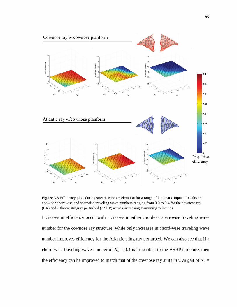
60

Figure 3.8 Efficiency plots during stream-wise acceleration for a range of kinematic inputs. Results are chow for chordwise and spanwise traveling wave numbers ranging from 0.0 to 0.4 for the cownose ray (CR) and Atlantic stingray perturbed (ASRP) across increasing swimming velocities.

Increases in efficiency occur with increases in either chord- or span-wise traveling wave

number for the cownose ray structure, while only increases in chord-wise traveling wave

number improves efficiency for the Atlantic sting-ray perturbed. We can also see that if a

chord-wise traveling wave number of Nc = 0.4 is prescribed to the ASRP structure, then

the efficiency can be improved to match that of the cownose ray at its in vivo gait of Nc =

61

0.2/Ns = 0.2, however this would come at the cost of increased adjacent radial strain (Fig

3.10) that exceed the measured strain thresholds reported in Chapter 2 (see Fig 2.9a).

Figure 3.9 Cruising economy plotsf the the steady-state regime of each structure over a range of kinematic inputs. Results are shown for chordwise and spanwise traveling wave numbers ranging from 0.0 to 0.4 for the cownose ray (CR) and Atlantic stingray perturbed (ASRP). The color represents the steady-state economy calculated from the cycle averaged power and steady-state velocity.

The effects of wave number manipulation on cruising speed and economy (Fig

3.9) reveal that increases in both chord- and span-wise wave number causes an increase

in cruising economy, but a decrease in cruising speed. The plots also show that for a

given selected cruising speed, the gait could be varied (in terms of chord- and span-wise

traveling waver number) to achieve the greatest economy for that speed.

It is important to keep in mind that increases in chord-wise traveling wave

number (Nc) correspond to exponential increases in adjacent radial strain Fig 3.10), and

at some point will exceed the physiological limits (see Fig 2.9a). If it is assumed that only

62

Figure 3.10 Adjacent radial strain plots as predicted by the biomechanical model for perturbation study 1. Each structure was exposed to a range of undulatory motions prescribed along the chordwise and spanwise directions. Wave numbers were varied between 0.0 and 0.4 to observe the point at which the strain becomes excessive (i.e., exceeds the measured strain limits).

gaits with corresponding strain levels at or below the tested physiological limits are

feasible, and that any feasible gait was available at any time during ray locomotion, then

we can see how variable gait selection could be used as means to maintain maximal

thrust and/or propulsive efficiency while staying within strain limits. The effect of gait

selection on adjacent radial strain levels, shown in figure 3.10, indicates that a gait with a

chord-wise traveling wave number up to 0.2, and a span-wise traveling wave number

over the full spectrum, could be selected without inducing excessive strain. Therefore it is

feasible that the gait could be continuously varied within these limits to maintain

63

maximal performance during the acceleration period. Figure 3.11 displays the velocity,

and efficiency-velocity trends for various gait selections that all correspond to acceptable

strain levels (see Fig 3.10). To test the effects of a continuously variable gait (CVG), a

simulation was run in which the chord- and span-wise traveling wave numbers were set

as high as possible (without causing excessive strain) then continuously decreased to zero

linearly with time over the first few cycles. The result is an efficiency curve (Fig 3.11b –

black dotted line) that runs just above the peaks of the feasible fixed gait simulations. We

also see that a plateau in thrust production can also be achieved (Fig 3.11a – black dotted

line). This result supports that CVG is effective in maintaining higher performance

across different swimming speeds, and is something that should be considered in a

vehicle design.

Figure 3.6 shows how the differences in joint displacement patterns translate to

differences in the maximum pitch angles, and subsequently performance. This shows that

the underlying structure design can be used as a mechanism for achieving increases or

64

Figure 3.11 Thrust and efficiency plots for feasible gaits which suggest the utility of variable gait for maximizing performance over a range of velocities. The black dotted line represents simulations of a continuously variable gait (CVG) case, in which the traveling wave numbers were linearly varied with time (from high to low), demonstrating the possible advantage variable gait control during the times of acceleration.

decreases in fin pitch angles, and therefore performance. However, Fig. 3.10 highlights

the induced strain consequences of these variations. Fig. 3.12 shows how the LE (Fig

3.12a) and TE (Fig 3.12b) pitch angles, and corresponding strain levels, are affected by

wave number manipulation for both the cownose ray and Atlantic sting-ray perturbed.

There is a strong difference in LE v. TE angles for the cownose ray across different wave

numbers, but not for the perturbed Atlantic sting-ray. We can also see that the maximum

65

Figure 3.12 Leading edge and trailing edge pitch angles for the cownose ray and Atlantic sting-ray perturbed. The corresponding average adjacent radial strain levels are also shown through color representation.

TE pitch angles for the cownose ray are much higher, with a peak of 42.15 degrees versus

17.07 degrees for the Atlantic sting-ray perturbed. Despite the much higher TE pitch

angles, however, the strain levels for each structure across the different wave number

66

combinations are predominantly equal with only slightly higher strains calculated for the

ASRP structure. The take away message from this analysis is that there are ways to

design an underlying fin structure that allows for a greater range of pitch angles, and

therefore performance, but without the accompaniment of high adjacent radial strain.

3.2.3 Perturbation study 2 over full test matrix

For perturbation study 2, chord-wise traveling wave numbers were varied as

reported in Table 3.2. Figure 3.13 shows that in terms of thrust production, the low speed

levels are almost identical but the cownose ray perturbed (CRP) thrust production drops

off more quickly that the Atlantic sting-ray. In terms of efficiency, we see that for the

highest wave number of 1.2, there is no advantage of the cownose ray perturbed over the

Atlantic sting-ray, and rather there is a disadvantage as velocity increases. However, as

wave number is decreased from 1.2 to 0.8, a trend similar to that seen in perturbation

study 1 is observed, where the low speed efficiency for the CRP structure is higher than

that of the ASR structure.

In terms of strain levels, Fig. 3.14 shows that both structures stay at or within the

tested strain limits for the Atlantic sting-ray (see Fig 2.9b), and decrease as wave number

decreases as expected. Slightly higher strain levels are seen for the ASR structure than for

the CRP structure, but both are within tested limits.

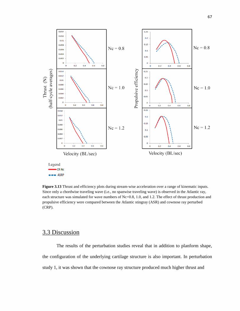
67

Figure 3.13 Thrust and efficiency plots during stream-wise acceleration over a range of kinematic inputs. Since only a chordwise traveling wave (i.e., no spanwise traveling wave) is observed in the Atlantic ray, each structure was simulated for wave numbers of Nc=0.8, 1.0, and 1.2. The effect of thrust production and propulsive efficiency were compared between the Atlantic stingray (ASR) and cownose ray perturbed (CRP).

3.3 Discussion

The results of the perturbation studies reveal that in addition to planform shape,

the configuration of the underlying cartilage structure is also important. In perturbation

study 1, it was shown that the cownose ray structure produced much higher thrust and

68

Figure 3.14 Adjacent radial strain plots as predicted by the biomechanical model for perturbation study 2. Each structure was exposed to a range of undulatory motions in the chordwise direction only with wave numbers varied between 0.8 and 1.2. The corresponding strain levels are shown for both the Atlantic sting-ray (ASR) and cownose ray perturbed (CRP).

achieved greater propulsive efficiencies than the ASRP structure, especially at the lower

velocities. The kinematic analysis of the three-dimensional airfoil shaped body explains

why these differences in performance occur, as much greater trailing edge pitch angles

along with chord-wise curvature was achieved by the cownose ray structure. Since the

differences were limited to the underlying structure configuration, we can conclude that it

is the design of the structure itself that is responsible. In Chapter 2, fanning angle, IRJP

angle, and planform were defined as the three skeletal design parameters that appeared to

have the greatest influence on fin construct. Since the planform was the same for both

structures, it follows that it must be the IRJP angle, fanning angle, or both that are

responsible for causing the differences in fin pitch angles, and subsequently swimming

performance. However, the results of perturbation study 2, where the cownose ray

structure was paired with the planform of the Atlantic ray, the benefits of the cownose ray

architecture are suppressed. This suggests that particular skeletal design features may

69

only be beneficial if paired with the right planform To reiterate the conclusions of chapter

2, it is further demonstrated in chapter 3 that the kinematic differences between the

cownose ray structure and the perturbed Atlantic (for the same prescribed chord- and

span-wise traveling wave numbers) occurs without any appreciable difference in adjacent

radial strain levels. It is this concept that is important to keep in mind when interpreting

the performance differences and using the results to inform AUV design.

In addition to the greater thrust predictions for the cownose ray, the model also

predicted that the source of thrust varies with kinematic differences, and therefore

ultimately the structural differences. The additional thrust contribution from the trailing

edge for the cownose ray structure, which was absent in the perturbed Atlantic ray

structure, may not only be important to achieving greater thrust, but may also be

important once the structural dynamics are considered. It is possible that this change in

the distribution of thrust production is important so that the total fluid loading acting on

the fin is not borne by one particular region of the fin (e.g., leading edge), but rather

distributed of a greater area. However, the addition of structural dynamic modeling would

be needed to address this issue.

The adjacent radial strain analysis across the entire test matrix (i.e., Nc and Ns

variations) shows that excessive strain requirement would limit the oscillating fins from

reaching high chord-wise traveling wave numbers. An Nc value above 0.2 causes strain

levels that begin to exceed the tested strain limits discussed in Chapter 2. Therefore we

can conclude that for the biological structures, the gaits would be constrained by a strain

threshold between adjacent radial elements. With regard to strain threshold, previous

work has discusses the presence of radial element bi-furcation [8], and can be seen in the

70

CT scans of Fig. 2.1. Since the higher stain levels occur toward the tip of the fins, which

is the same area where bi-furcation is found, it is hypothesized that bi-furcation could be

a mechanism for increasing the strain threshold, and subsequently increasing the feasible

gaits for a given structure. Modeling in radial element bi-furcation and investigating the

effect of it of strain level is an area for future work. The results on efficiency and thrust

production show how gait manipulation could be used as a mechanism for maintaining

maximal performance output across a range of swimming velocities. Although this is an

interesting insight into biology alone, the concept of continuously variable gait (CVG) is

an important idea that should be considered when designing artificial systems for AUVs.

If a vehicle mission requires frequent changes in speed and direction, then having CVG

capability might be extremely important and investigating ways to achieve this artificially

would be recommended.

Although the results of chapter 3 show that the skeletal architecture does

influence performance, the effects of each skeletal parameter (e.g., IRJP angle, fanning

angle) on performance should be studied independently; where differences in structure

designs can be better controlled, with changes in fin design confined to the manipulation

of a single parameter value. Therefore in chapter 4, a parameterized modeling approach is

introduced and to study demonstrate how each parameter influences performance

independently.

71

Chapter 4

Parameterized modeling of ray-like skeletal structures

A parameterized approach to modeling ray-like skeletal structures is presented,

which allowed for the influence of the previously identified skeletal design parameters to

be studied independently, and in a systematic fashion. The fluid-structure analysis

presented in the previous chapter focused on the real skeletal structures of the cownose

and Atlantic rays, which are extremely complex and would not be feasible to replicate

synthetically. If the principles behind the biomechanics of rays are to be leveraged in the

design of artificial systems, it is important to understand how the skeletal design

parameters (discussed in chapter 2 and highlighted in Fig 2.1) impact performance

independently. Only then can we identify which parameter is most important when trying

to reproduce a particular performance outcome. In this chapter, a parameterized approach

to modeling ray-like skeletal structures is introduced which allows the influence of the

previously identified skeletal design parameters to be studied independently, and in a

systematic fashion. To facilitate this study, a numerical model was developed to generate

artificial structures that were similar in complexity to the real biological rays skeletons

(i.e., similar number of radial elements and joints). The parameterized model was also

designed to generate simplified structures with many fewer radial elements and joints that

can be designed and fabricated for experimenting with artificial systems. Therefore, this

chapter is two-fold, involving parameterized modeling to quantify the effects of skeletal

72

parameter manipulation on hydrodynamic performance, as well as a bio-inspired design

component in which the numerical modeling is used to inform the design of simplified

structure. The specific objectives of chapter 4 were to 1) quantify the effects of skeletal

design parameters, including IRJP and fanning angle, on swimming performance

on complex fins that are comparable to biology, 2) determine if performance

advantages related to these parameters hold for simplified structures that can be

built, and 3) test the modeling insights through the design of functional artificial

structures, for hydrodynamic experimentation.


4.1.1 Parameterized model development

The parameterized model was designed to generate “ray-like” skeletal structures

of various levels of complexity. The inputs are desired number of radial elements, R,

desired number of segments of the longest radial element, S (i.e., root-to-tip mid-chord),

IRJP angle (𝛾), fanning angle (𝜁), and planform shape (𝚾). The output of the model is a

set of (x,y) coordinates representing initial joint positions. In Chapter 2, the initial joint

coordinates 𝑼𝑟𝑠(0), introduced in equation (4), was obtained directly from biology via

the CT reconstructions, in which 𝛾, 𝜁,𝚾 were inherent to the cartilage structure (see Fig.

2.3). In this parameterized case, however, the skeletal parameters are prescribed such that

𝑼𝑟𝑠(0) = 𝑓( 𝛾, 𝜁,𝚾), and was calculated from the following:

73

𝑮𝑟𝑠 = 𝑓�𝐿𝑠𝑝𝑎𝑛, 𝐿𝑐ℎ𝑜𝑟𝑑�, 𝑤ℎ𝑒𝑟𝑒 𝐆𝑟𝑠 ∈ ℝ2

𝑮𝑥𝑠 = ∀𝑠: [0 ∆𝑥 2∆𝑥 3∆𝑥 ⋯𝐿𝑐ℎ𝑜𝑟𝑑]𝑇

,𝑤ℎ𝑒𝑟𝑒 ∆𝑥 = 𝐿𝑐ℎ𝑜𝑟𝑑𝑅

𝑮𝒚𝑟 = ∀𝑟: .25𝐿𝑠𝑝𝑎𝑛 + [0 ∆𝑦 2∆𝑦 3∆𝑦 ⋯𝐿𝑠𝑝𝑎𝑛]

,𝑤ℎ𝑒𝑟𝑒 ∆𝑦 = 𝐿𝑠𝑝𝑎𝑛𝑆

𝑮𝑠′ = 𝛺2(𝛾𝑠) ∙ 𝑮𝑠 ,𝑤ℎ𝑒𝑟𝑒 𝛾𝑠 = [0 ∆𝛾 2∆𝛾 3∆𝛾 ⋯𝛾𝑚𝑎𝑥]𝑇

,𝑎𝑛𝑑 ∆𝛾 = 𝛾𝑚𝑎𝑥𝑆

𝑮𝑟′ = 𝛺2(𝜁𝑟) ∙ G𝑥𝑦𝑟 ,𝑤ℎ𝑒𝑟𝑒 𝜁𝑟 = [−𝜁𝑚𝑎𝑥 −(𝑅 − 1)∆𝜁 ⋯0 ∆𝜁 2∆𝜁 ⋯𝜁𝑚𝑎𝑥]

,𝑎𝑛𝑑 ∆𝜁 = 2𝜁𝑚𝑎𝑥𝑅

𝑼𝑟𝑠𝑥𝑦(0) = [𝐆𝑟𝑠′ ∩ 𝚾 ], and 𝑼𝑟𝑠

𝑧 (0) = 0, 𝑤ℎ𝑒𝑟𝑒 𝑤ℎ𝑒𝑟𝑒 𝑼𝑟𝑠 ∈ ℝ3

where 𝛾𝑚𝑎𝑥 and 𝜁𝑚𝑎𝑥 are the prescribed values to define the desired IRJP angle and

fanning angle, respectively, and 𝚾 ∈ ℝ2 , and is a matrix containing vertices in (x,y) that

defines the planform shape.

Figure 4.1 illustrates the parameterized modeling process in which the joint

pattern inputs are selected (Fig. 4.1 – step 1), then used to generate a grid of points that

will function as joint locations (Fig. 4.1 – step 2), on which a desired planform shape is

sketched overtop of the grid (Fig. 4.1 – step 3), and finally the points that fall outside of

the planform are filtered out leaving behind a matrix of joint positions that defines an

(4.2)

(4.1)

(4.6)

(4.5)

(4.4)

(4.3)

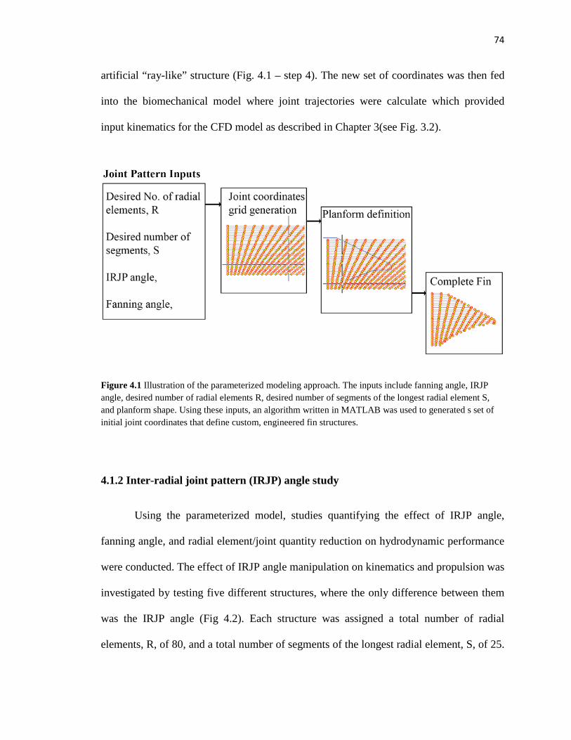
74

artificial “ray-like” structure (Fig. 4.1 – step 4). The new set of coordinates was then fed

into the biomechanical model where joint trajectories were calculate which provided

input kinematics for the CFD model as described in Chapter 3(see Fig. 3.2).

Figure 4.1 Illustration of the parameterized modeling approach. The inputs include fanning angle, IRJP angle, desired number of radial elements R, desired number of segments of the longest radial element S, and planform shape. Using these inputs, an algorithm written in MATLAB was used to generated s set of initial joint coordinates that define custom, engineered fin structures.

4.1.2 Inter-radial joint pattern (IRJP) angle study

Using the parameterized model, studies quantifying the effect of IRJP angle,

fanning angle, and radial element/joint quantity reduction on hydrodynamic performance

were conducted. The effect of IRJP angle manipulation on kinematics and propulsion was

investigated by testing five different structures, where the only difference between them

was the IRJP angle (Fig 4.2). Each structure was assigned a total number of radial

elements, R, of 80, and a total number of segments of the longest radial element, S, of 25.

75

This was chosen as it closely approximated the totals observed in the real cownose ray

structure, where R=87 and S=26. The IRJP angle was varied from 0 degrees to 50 degrees

by increments of 12.5 degrees. The planform shape was held constant (i.e., 𝚾 ≠ 𝑓(𝛾, 𝜁) )

and was taken from the cownose ray.

Figure 4.2 Method for examining the effect of the inter-radial joint pattern (IRJP) on kinematics and propulsion. Five structures were generated using the parameterized model, and fluid structure simulations were run over a range of chordwise and spanwise traveling wave numbers, ranging from 0.0 to 0.4.

As conducted in chapter 3, free-swimming simulations were run for each structure

over a range of kinematics inputs. The test matrix used for this study was the same as that

used in perturbation study 1, and is displayed in Table 3.1. The performance effects of

increasing the IRJP angle (𝛾), were analyzed using the same methods presented in the

perturbation studies of chapter 3, in which thrust production, propulsive efficiency,

cruising speed, and cruising economy were calculated. The kinematic effects were also

analyzed using the same methods of Chapter 3, in which the LE and TE pitch angles were

calculated and correlated with IRJP angle. As done in perturbation study 1, this kinematic

analysis included the consequences on adjacent radial strain as a function of IRJP angle

and prescribed motions.

76

4.1.3 Fanning angle study

The effect of fanning angle(𝜁) on performance was investigated by comparing

five identical structures but with increasing levels of fanning angle. The fanning angle

was varied between 0 degrees and 80 degrees by increments of 20 degrees; where for

example, a fanning angle of 80 degrees means that the total range of fanning angle from

leading edge to trailing edge is 160 degrees, starting at +80 degrees for the leading most

radial element, and ending at -80 degrees at the trailing most radial element, measured

relative to the span-wise axis. This compares with the fanning angle range and

distribution of the real Atlantic ray of a leading edge start angle of approximately + 104

degrees, and a trailing edge end angle of approximately -83 degrees, corresponding to a

total fanning angle range of approximately 187 degrees. The 80 degree limit was chosen

because as 90 degrees is approached the radial element will begin to overlap each other

on a single line, and would cause numerical errors in the fluid-structure mapping

algorithm. The effect of fanning angle manipulation on performance was examined using

the same approach as the IRJP angle study.

Figure 4.3 Method for examining the effect of the fanning angle on kinematics and propulsion. Fie structures were generated using the parameterized model, and fluid structure simulations were run in the in vivo kinematics of the cownose ray prescribed.

77

4.1.4 Simplified structure study

As the ultimate objective of this work is to inform the design of AUV propulsion

systems, a study was done to investigate whether or not the biological features observed

in the real ray skeletal structures are applicable to simplified structures that could be used

in an underwater vehicle. The IRJP angle was chosen as the parameter to test on

simplified structures as it was determined that this could be most easily replicated and

tested in an artificial fin, allowing for comparisons between modeled fins and artificial

fins to be made. As done in the complex study, the IRJP angle was increased from 0

degrees to 50 degrees. Three structures were tested, 0, 25, and 50 degrees. The analysis

method for the complex study was again used in the simplified structure study.

Figure 4.4 Method for examining the effect of the inter-radial joint pattern (IRJP) on kinematics and propulsion for simplified structures with the potential for manufacture. Three structures were generated using the parameterized model, and fluid structure simulations were run for select prescribed motions.

78

4.2 Results – (parameterized modeling FSI)

4.2.1 IRJP angle study results

- in vivo prescribed kinematics (cownose ray)

To begin analyzing the effect of IRJP angle on performance, preference was given

to the case in which the in vivo kinematics of the cownose ray, discussed in chapter 2,

were prescribed where the chord- and span-wise traveling wave numbers were both set to

0.2 waves. Simulations were run on all five structures to show that an increase in IRJP

angle directly alters performance. Figure 4.5 shows that increasing the IRJP angle

increases the thrust production for the lower speeds of about 1.0 BL/sec or less (Fig 4.5a).

Increases in low speed propulsive efficiency were also observed (Fig 4.5b). Cruising

speeds decreased with increasing IRJP angle (Fig 4.5c) with a peak in cruising economy

occurring for the structure with an intermediate IRJP angle of 25 degrees. The velocity

trajectory plots for the extremes (i.e., 0-deg and 50-deg IRJP angles, Fig 4.5d) show that

the structure with the maximum IRJP angle behaves similarly to the real cownose ray

structure with the same prescribed motions, where the 0-deg IRJP angle structure behaves

very similar to the Atlantic sting-ray perturbed structure (see Fig 3.3a).

The results of perturbation study 1, discussed in chapter 3, demonstrated similar

results of increased low speed performance (see Fig 3.3). It was also shown that the

cownose ray structure, which has an IRJP angle of approximately 52° degrees, was

getting additional thrust contribution from the trailing edge. Figure 4.6 shows how

increasing the IRJP angle has the same effect of gaining additional thrust contribution

79

Figure 4.5 Performance plots for the IRJP study for the natural gaits observed for the cownose ray. Simulations were run for a chordwise and spanwise traveling wave number of 0.2. Thrust and propulsive efficiency are plotted for stream-wise free swimming cases. The performance for three structures is shown to demonstrate the relationship between increasing IRJP angle and low speed thrust production and efficiency. Five structures were computationally tested with IRJP angles ranging from 0 to 50 degrees.

80

from the trailing edge (Fig 4.6b). It is also shown that added drag at the trailing edge also

occurs to the structures with higher IRJP angles (Fig 4.6c), which agrees with the results

of perturbation study 1 (see Fig 3.4c).

Figure 4.6 The effect of increasing IRJP angle from 0 to 50 degrees (a) on altering the source of thrust production (b,c). The plots show the distribution of thrust forces where red corresponds to high positive thrust and blue to negative thrust (i.e., high drag). Both isometric (b) and lateral (c) views are shown.

Increasing the IRJP angle had the effect of increasing trailing edge pitch angles,

which was consistent with the results of perturbation study 1. Figure 4.7a shows the

relationship between increasing IRJP angle and changes in leading and trailing edge pitch

angles. The leading edge pitch angles remain relatively unchanged, while the trailing

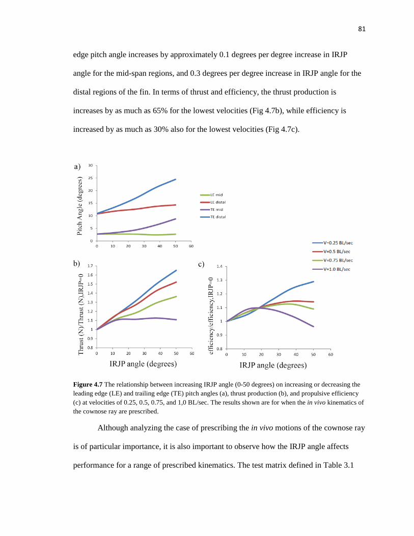
81

edge pitch angle increases by approximately 0.1 degrees per degree increase in IRJP

angle for the mid-span regions, and 0.3 degrees per degree increase in IRJP angle for the

distal regions of the fin. In terms of thrust and efficiency, the thrust production is

increases by as much as 65% for the lowest velocities (Fig 4.7b), while efficiency is

increased by as much as 30% also for the lowest velocities (Fig 4.7c).

Figure 4.7 The relationship between increasing IRJP angle (0-50 degrees) on increasing or decreasing the leading edge (LE) and trailing edge (TE) pitch angles (a), thrust production (b), and propulsive efficiency (c) at velocities of 0.25, 0.5, 0.75, and 1,0 BL/sec. The results shown are for when the in vivo kinematics of the cownose ray are prescribed.

Although analyzing the case of prescribing the in vivo motions of the cownose ray

is of particular importance, it is also important to observe how the IRJP angle affects

performance for a range of prescribed kinematics. The test matrix defined in Table 3.1

82

was applied again in the IRJP angle study and effects of IRJP angle for various input

motions were simulated. Figure 4.8 shows the thrust production at three different

velocities for three structures differing only by IRJP angles of 0-deg, 25-deg, and 50-deg.

This includes the two structures at the extremes as well as the intermediate IRJP angle

structure. Results shows a dramatic increase in low speed thrust production with

increasing IRJP angle, and also shows how the gait could be adjusted as velocity

increases to maintain peak thrust production. It was further shown that with proper gait

selection, the structure with the highest IRJP angle of 50-deg can match the thrust

production of the other structures, indicating that when coupled with variable gait control,

the 50-deg IRJP angle structure provides the best performance over the greatest range of

swimming speeds. The effect on propulsive efficiency over a range of motions is shown

in Fig. 4.9, where the structure with 0-deg IRJP angle has lower all around low speed

efficiency than the structure with a 50-deg IRJP angle, but is more efficient overall at the

highest sampled velocity of 1.5 BL/sec.

Once steady-state velocity was reached, the cruising speed and cruising economy

were evaluated over the same range of motions as for the thrust and efficiency analysis.

Figure 4.10 displays both the cruising speed and economy for the two extreme and

middle structures for a range of wave number combinations. As seen in the perturbation

studies, the highest cruising speed occurs at the lowest wave numbers, but this is also

83

Figure 4.8 Thrust plots during streamwise acceleration for a range of kinematic inputs. Results are shown for the chord wise and spanwise traveling wave numbers ranging from 0.0 to 0.4 for artificially generated structures with increasing IRJP angles of 0, 25, and 50 degrees. The color represents the thrust force produced across increasing velocities of 0.5 BL/sec (a), 1.0 BL/sec (b), and 1.5 BL/sec (c).

84

Figure 4.9 Efficiency plots during streamwise acceleration for a range of kinematic inputs. Results are shown for the chord wise and spanwise traveling wave numbers ranging from 0.0 to 0.4 for artificially generated structures with increasing IRJP angles of 0, 25, and 50 degrees. The color represents the thrust force produced across increasing velocities of 0.5 BL/sec (a), 1.0 BL/sec (b), and 1.5 BL/sec (c).

85

where the lowest economy occurs. It is difficult to draw conclusions about which fins are

more economical than others if their respective cruising speeds are different. However,

the plots in figure 4.10, if comparisons are made for a single velocity, for example 1.5

BL/sec, we can see that for that velocity, the middle structure is considerably more

economical. This is especially true when combined with the optimal gait selection, such

as the middle structure with an Nc/Ns combination of 0.4/0.0.

Figure 4.10 Cruising economy plots for the steady-state regime for identical fins but with increasing IRJP angle. Results are shown for the chordwise and spanwise traveling wave numbers between 0.0 and 0.4 for the structure with 0-deg, 25-deg, and 50-deg IRJP angles. The color represents the steady-state economy calculated from the cycle averaged power and steady-state velocity.

In the analysis of the in vivo prescribed motions of the cownose ray, it was shown

that increases in IRJP angle lead to increases in trailing edge pitch angles of the fin.

However this was only shown for one prescribed motion and not for the full test matrix.

It was shown in perturbation study 1 that both internal cartilage patterns (e.g., IRJP) and

wave number combinations are important in determining fin pitch angles. It was also

shown how the adjacent radial strain is affected by the same thing. Therefore an analysis

86

on the effect of increasing IRJP angle on leading/trailing edge pitch angle, and adjacent

radial strain was conducted. Figure 4.11 shows the leading edge (LE) and trailing edge

(TE) pitch angles, as well as the corresponding impact of adjacent radial strain. The strain

is reported as the average over the entire fin. The average values are generally much

lower than the peak strain levels, but was found to be a good metric for analyzing how

changes in skeletal architecture and prescribed motion increase or decrease strain levels.

From figure 4.11, we can see that increases in IRJP angle causes increases in both

LE and TE pitch angles, but increases TE pitch angle at a much greater rate. The LE pitch

angles were observed in increase with IRJP angle at approximately 0.2 degrees per

degree increase in IRJP angle, as compared to 0.4 degrees increase in TE pitch angle per

degree increase in IRJP angle, which is nearly double the rate of increase of the LE pitch

angle. It is also important to note that the LE and TE pitch angle is the same for the 0-deg

IRJP angle structure, but is not the same for the 25 and 50-deg IRJP angle structures. For

the 25-deg structure, the pitch angle increase by about 5 degrees between the leading and

trailing edge, and by about 10 degrees between leading and trailing edge for the 50-deg

structure. This implies that chord-wise curvature occurs when the IRJP angled is

increases above zero, where the amount of curvature is positively correlated with IRJP

angle. With an increase in the difference between leading and trailing edge pitch angles

of 0 degrees for the 0-deg structure, to 10 degrees for the 50-deg structure, the difference

in leading and trailing edge pitch angle is proportional to IRJP angle by a factor of .2

degrees per degree increase in IRJP angle.

87

Figure 4.11 Leading edge (LE) and trailing edge (TE) pitch angles as a function of increasing IRJP angle, and compared to the corresponding average strain levels for different prescribed motions. Results are shown for chordwise and spanwise traveling wave numbers ranging from 0.0 to 0.4 for identical structures but with increasing IRJP angles. The color represents the average adjacent radial strain that corresponds to each wave number combination.

4.2.3 Fanning angle study results

The results of the fanning angle study, presented in Fig. 4.12, show that

increasing the fanning angle seems to cause an increase in overall thrust production

across all velocities up to steady-state, up until the 60-deg fanning angle structure, at

88

Figure 4.12 Performance plots for the fanning angle study for the natural gait of the cownose ray. Simulations were run for a chordwise and spanwise traveling wave number of 0.2. Thrust and propulsive efficiency are plotted for free swimming cases. Five structures were computationally tested with fanning angles ranging from 0 to 80 degrees by increments of 20 degrees.

89

which point the thrust dropped off suddenly between the 60 and 80-deg structure (Fig

4.12a). When comparing the extremes, however, the structure with 0-deg fanning angle

produces slightly higher low speed thrust, with the 80-deg structure slightly higher at the

higher velocities. The efficiency decreased with increasing fanning angle for all

structures at the lower velocities, with slight advantages in efficiency at the higher

velocities as fanning angle increased. In terms of cruising speed and economy, the speed

increased with increasing fanning angle while the economy decreased, but again only up

until the 60-deg structure (Fig 4.12c). When comparing the velocity trajectories of the

two extreme structures (i.e., 0-deg and 80-deg fanning angle, Fig 4.12d), a slight

advantage in acceleration is seen for the 0-deg structure over the 80-deg structure, but the

80-deg structure eventually reaches a higher velocity. This result is similar to that seen in

perturbation study 1, but with much less of a difference between the two structures. It is

hypothesized that this happens because the 0-deg structure is closer to the cownose ray

design, while the 80-deg structure is closer to the Atlantic sting-ray perturbed design, but

they are not different enough to cause for the same magnitude in performance differences

as seen in perturbation study 1.

4.2.3 IRJP angle study for simplified structure results

The IRJP angle study for the simplified structures revealed that the effect of

increasing the IRJP angle still holds for structures with only 10 radial elements, and 5

mid-chord segments, versus 80 and 25 for the complex counterparts, respectively. Fig.

4.13 shows that increasing the IRJP angle translates to increases in low speed thrust

production (Fig. 4.13a) and efficiency (Fig. 4.13b), just as was observed for the complex

fins.

90

Figure 4.13 Performance plots for the IRJP study for the simplified structures for chordwise and spanwise traveling wave numbers of 0.2. Three structures were studied with results demonstrating that even for simplified structures, an increasing IRJP angle can lead to increases in low speed thrust production and propulsive efficiency.

91

However, the level of increase in relation to IRJP angle increase was considerably less

than that for the complex fins. Figure 4.14 shows the comparison in the effect of IRJP

angle on LE and TE pitch angles for both the complex and simplified structures. The

corresponding effect on thrust production and propulsive efficiency is also reported. The

results support the idea that the biological design features can indeed be leveraged in the

design of simplified, biomimetic structures that function in a similar way as the real

biological systems. However, the influence of particular skeletal parameters on

performance, such as the IRJP angle, is shown to be sensitive to fin complexity level (i.e,

total number of radial elements and joints). Figure 4.14 shows the comparison between

the complex and simplified fin pitch angles (Fig 4.14a), thrust production (Fig 4.14b),

and propulsive efficiency (Fig 4.14c). The performance gain of increasing IRJP angle,

though still present for the simplified structures, was reduced along with the reduction in

total number of radial elements and joints. In terms of thrust production, the maximum

increase in thrust production for the lowest velocity (0.25 BL/sec) was 65% for the

complex structure as compared to 44% for the simplified structure. As velocity increases,

this becomes 52% for the complex structure and 29% for the simplified structure at 0.5

BL/sec, 36% for complex and 10% for simplified at 0.75 BL/sec, and 10% versus -4% at

1.0 BL/sec. These results show that though the boost in thrust production with increasing

IRJP angle does still occur for simplified structures, the advantage was lessened for the

lowest velocities, and disappears completely at some of the higher velocities as indicated

by the 10% versus -4% changes in thrust production for the complex versus the

simplified structure at 1.0 BL/sec. The explanation for this can be found in the leading

and trailing edge pitch angle analysis for both the complex and simplified structures and

92

Figure 4.14 Comparisons between the effects of IRJP angle on kinematics and propulsive for complex and simplified fin structures. The relative difference in LE and TE pitch angles are also shown (a), as well as the comparison of IRJP angle effects of thrust production (b), and propulsive efficiency (c).

how they compare (Fig 4.14a). The pitch angles are close to the same for the mid-span

regions (Fig 4.14a – green & magenta). For the distal fin regions, however, the maximum

LE pitch angle was 14.3 degrees for the complex, 50-deg IRJP angle structure, versus

10.5 degrees for the simplified, 50-deg IRJP angle structure. The TE pitch angle for the

distal regions was 24.5 degrees for the complex, 50-deg IRJP angle structure, as

compared to 20.1 degrees for the simplified structure. This correlates to a 27% difference

in LE pitch angle, and 18% difference in TE pitch angle.

93

4.3 Discussion

The parameterized modeling results show that there is a clear cause and effect

between IRJP angle and performance. The model shows that by increasing the IRJP

angle, the leading edge and trailing edge pitch angles can be increased without changing

the input chord- and span-wise traveling wave numbers. In addition to increasing these

angles, the IRJP angle induces chord-wise curvature where the leading edge and trailing

edge pitch angles are not equal. This change in kinematics caused increases in low speed

thrust production and propulsive efficiency (see Fig. 4.8, 4.9), as well as a redistribution

of the source of thrust production throughout the fin (see Fig 4.6). Furthermore, the effect

on IRJP angle on cruising performance shows how particular combinations of chord- and

span-wise traveling wave number can be paired with the right structure to achieve peak

cruising economy for a selected cruising speed (see Fig 4.10). For example, the middle

structure (i.e., 25-deg IRJP angle) demonstrated the best overall economy, but with the

proper gait selection, the other structures can function at similar economy level. Of

course, the performance gains of the higher IRJP angle structure should be considered as

well. For instance, if the greater low speed thrust production is a priority over cruising

economy, then the 50-deg IRJP angle structure would be a better option. However, if

economy takes precedence, then the 25-deg structure offers the best performance. It is

this type of trade off that would need to be considered when selecting a fin design and

with a quantitative description of how IRJP angle influences performance, mathematical

descriptions equating structural features to performance can be derived and used in

designing new fins to achieve a desired performance outcome.

94

The fanning angle study did reveal that manipulating this parameter can alter

performance, but there is no clear advantage for oscillating fins. Although the model

shows that the thrust production increased slightly with increasing fanning angle,

decreases occurred for both efficiency and economy, demonstrating that the fanning

angle was not the parameter most effective for improving performance for the oscillating

fins. Instead, the IRJP angle was more effective, and can be manipulated to predictably

alter performance. Since structures in nature with high fanning angles tend to be

undulating ones, the benefit of increasing the fanning angle may only present itself for

undulating structures with more circular planforms. This is an area for future

investigation.

The results of examining the IRJP angle effects on simplified structures shows

that the features of ray skeletal architecture can not only work for the complex biological

fins, but also for simplified fins with many fewer radial elements and joints that could

actually be built and tested. However, the results also demonstrated that the amount of

performance gain, in correlation with increasing IRJP angle, was reduced as the quantity

of radial elements and joints was reduced. Although the performance advantages of IRJP

angle were less for simplified structures (see Fig 4.14b,c), they are still considerable, and

the choice of whether or not to take advantage of this in the design of an artificial system

will depend on how important the performance advantage is for a given vehicle mission.

The modeling suggest that the way pectoral fin structures are built in nature could

still function for artificial fins, where essentially simplified versions of the biological

structures are designed and fabricated for use in an underwater vehicle. In chapter 4, this

idea will be investigated through an experimental approach to testing artificial pectoral

95

fins with simplified skeletal structures functioning to actuate the fin to generate

propulsion. The results of the IRJP angle study for simplified fins suggests that not only

can simplified structures still perform well, but the effects of skeletal parameter

manipulation on performance can work as well. An experimental approach to confirming

this hypothesis is introduced in Chapter 5, and IRJP angle tests on real, physical

structures, are conducted.

96

Chapter 5

Bio-inspired design of artificial pectoral fin skeletal system

The results of chapter 4 demonstrate how the skeletal design parameters influence

kinematics and hydrodynamic performance for both complex structure like those of real

rays, and simplified structures that can be manufactured and potentially used for an

underwater vehicle. As the motivation for this work is to advance underwater vehicle

technology, it is important to not lose sight of our overall objective, which is to study

nature’s propulsion systems, learn from them, and apply the lessons learned to the design

of artificial systems for use in AUVs. Therefore, this chapter introduced an approach to

designing and fabricating artificial structures inspired by the anatomy of real ray

skeletons and to test the viability of that design methodology in underwater vehicle

propulsion. The modeling results for the simplified structures discussed in Chapter 4

supported the idea that not only can these be used to reproduce the performance of rays,

but also that the advantages of skeletal design parameter manipulation can still hold for

these simplified ones. Furthermore, the IRJP analyses of chapter 4 showed that the

increase in low speed performance, as a function of an IRJP angle increase, can work for

both complex and simplified structures (see Fig 4.14). However, without experimentally

testing this hypothesis, it is difficult to draw conclusions with confidence. The objectives

of chapter 5 were to: 1) develop a design and fabrication method for constructing and

testing ray-inspired artificial skeletal structures, and 2) experimentally test the

97

value of skeletal design parameter manipulations for artificial structures by testing

two artificial structures with different IRJP angles.

5.1 Materials and Methods (Chapter 5)

5.1.1 Artificial structure design and actuation platform

In order to maintain connectivity with the numerical modeling, the design

approach for the artificial systems was to create artificial biomimetic structures where the

individual components were direct artificial counterparts of real ray anatomical features.

As discussed in chapter 2, the ray fin consists of a series of cartilage segments connected

in series by joints to form radial elements (see Fig 2.1). Therefore, artificial segments

were designed and connected in series by joints to form artificial radial elements. The

total number of elements and joints was decided based on the numerical modeling results

from chapter 4 on the simplified structures, in which 10 radial elements were used with a

design target of 5 segments included in the mid-chord radial element.

The individual cartilage segments of the biological structures (Fig 5.1a), were

used as inspiration for artificial segments (Fig 5.1b). The artificial segments were

designed using SolidWorks computer aided design (CAD) software, and manufactured on

a Dimension sst 1200es 3D printer. The segments were designed to be hinge-jointed

together in series using 4-40 Stainless Steel axle bolts (Fig 5.1c). By controlling the total

number of segments connected, and the length of each segment, radial element length of

was set as desired.

98

Figure 5.1 Design and fabrication of an artificial ray pectoral fin musculoskeletal system to experimentally study fluid structure mechanics. The hinge jointed cartilage segments found in the real biological fins (a), were used as inspiration for designing artificial segments (b). The segments were designed using SolidWorks, manufactured on a Dimensions 1200es 3D printer, and linked together to form artificial radial elements (c). The cross-bracing between the radial elements (a) was synthesized using O-ring chord stock elastomer with the same done above and below each radial element (d). The radial elements were mounted to a root structure and repeated chordiwse to form the whole structure (e).

99

The connections between the radial elements (i.e., cross-bracing, see Fig. 5.1a, Fig. 2.1b)

were established by running O-ring chord stock (Fig. 5.1d) through holes designed into

the middle area of each segment (Fig. 5.1b), which extended all the way from the leading

edge to the trailing edge. The assembly of 10 radial elements was then mounted to a rigid

root structure which was also manufactured using a 3D printer (Fig. 5.1e). The design

allowed for span-wise curvature to be achieved through radial element joint rotation, just

as in the biomechanical model, and also allowed for chord-wise undulation to be

accomplished to phase control between adjacent radial elements. Since the artificial

cross-bracing (i.e., O-ring chord stock) is elastic, adding undulations into the system

leads to the development of strain between the radial elements in the same way as the the

biological structures of real ray. Designing the artificial structure such that the individual

components had direct biological counterparts was an effective approach to ensure

connectivity with the numerical modeling was maintained.

To actuate the structure, a rotary-based cable drive system was integrated with the

artificial skeletal structure. Cables were run along the top and bottom of each radial

element and attached to the proximal end of the segments. A cable attachment point was

positioned at the top and bottom of each segment, translating to a total number of cables

per radial element to be equal to the total number of joints in the radial element (Fig 5.2).

The fin structure was then mounted to a custom built aluminum chassis designed to house

10 independently controlled rotary actuators, providing independent control of each

radial element (Fig 5.2a).Ten Hitec HS-7245MH hobby servos (Fig 5.2c,

www.hitecrcd.com) were selected as the actuator units and were used to drive custom

cable drive wheels. Multiple cables were attached to a single drive wheel (ranging from

100

one to five cables depending on the number of segments in the radial element being

actuated), routed through guide holes designed into the root structure, then attached to the

individual segments using copper cable crimps (Fig 5.2b,d). The servo control and power

was delivered using a Parallax Propeller controller USB unit with P8X32A-M44

Propeller chip on-board with 80 MHz clock speed, 64KB EEPROM, and 16 channels

(Fig 5.2e).

5.1.2 Structure motion control

Control signals were generated using the biomechanical model which calculated a

target set of time varying joint angles for the artificial structures; a process developed for

simulating the motion of biological structures, and is described in Chapter 2 and

illustrated in Fig. 2.2. Once the target set of joint angles was calculated, a kinematic

modeling approach was used to convert time-position signal controlling joint angles, to a

time-position signal for the servo wheel control that would be required to achieve the

same target set of joint angles for the artificial structure. In real rays, muscle fascicles

(i.e., individual contractile elements) run long the top and bottoms of every radial element

[8,56]. To model this, moment arms were introduced to each segment extending above

and below each segment’s proximal joint. The cable routing was modeled as line

segments which ran above and below each radial element from root to tip and was

attached to the underlying structure through moment arms. The kinematics of the

underlying structure was extended to solve for the time varying displacement of cable

attachment points. The information on the structure geometry and joint angles were

101

Figure 5.2 System integration to achieve a structure that can be actuated a tested. The structure was assembled as illustrated in figure 5.1 then attached to an airfoil shaped root structure and mounted to an aluminum chassis (a). Ten Hitec HS-7245MH servos (c) were mounted to the frame with attached tapering wheel cranks for driving multiple cables (d). Cables were routed through the root structure (d) and attached to the individual segments to actuate the structure (b). Servo control was provided by a 16 channel Parallax Propeller controller (e) with USB interface to receive instructions generated by Labview.

102

provided by the biomechanical model and combined with matrix based multi-body

mechanics to solve for cable attachment point displacement as follows:

𝐸𝑟𝑠(𝑡) = 𝛺3�𝜃𝑟𝑠(𝑡)� 𝛺3(𝛽𝑟𝑠)𝐼3

𝑴𝑟𝑠(𝑡) = 𝑼𝑟𝑠(𝑡) + 𝑚𝑟𝑠 𝐸𝑟𝑠(𝑡)𝑇 ∙ �̂�𝑧

from which the required amount of cable travel to achieve the target set of joint angles

𝜃𝑟𝑠(𝑡), and was calculated from:

𝐶𝑟𝑠(𝑡) = ∑ 𝑴𝑟𝑠(𝑡)𝑠1 , 𝑒𝑣𝑎𝑙𝑢𝑎𝑡𝑒𝑑 𝑓𝑟𝑜𝑚 𝑟 = 1 𝑡𝑜 𝑟 = 𝑅

where 𝐶𝑟𝑠 is the amount of required cable travel for the cable connected to radial segment

s of radial element r.

The final step in the conversion of joint rotation to servo wheel rotation involves

using the cable travel lengths to solve for the amplitude of oscillation of the servo wheel

required to give rise to the target joint angles, 𝜃𝑟𝑠 (𝑡) . Using the calculated cable travel

required for the longest radial element, which has 5 segments in this case, the amplitude

of oscillation for the servos is solved by:

𝐴𝑟𝑠𝑒𝑟𝑣𝑜 = ∀ 𝑠: 𝐶𝑟𝑠𝑏𝑠

where b is the radius of the servo crank wheel that is driving the cable attached to

segment s. Since there was only one actuator per radial element, then only one amplitude

(5.1)

(5.2)

(5.3)

(33)

103

Figure 5.3 Process of using the biomechanical model to solve for the amount of required cable travel to achieve desired amplitude of flapping. Line segments representations of muscle are attached to each radial element in the whole structure (a), and run along the top and bottom (b). The line segments shorten as joint rotation occurs, and the shortening length is equated to cable travel. The cable travel, in combination with the radii of the tapered servo wheel (d), is used to solve for the servo wheel angular amplitude.

value could be used for driving all segments within the radial element. However the

amount of cable travel required for each segment varies depending on the segment

position relative to the fin root. To accommodate this, the servo crank wheel was tapered

with a variable pulley radii, which was smallest for the most proximal segment cable, and

increased linearly to the largest radius pulley used for driving the cable attached to the

distal-most segment. A constant moment arm was used for all segments in the fin

structure to simplify the cable drive system and allow for the wheel radii to increase

linearly from the cable driving the root segment to the cable driving the tip segment.

In addition to amplitude control, the ability to actively undulate the fin was

achieved through phase control over the oscillatory motion of adjacent radial elements.

The phase was solved just as done in the biomechanical model (see Eq. 2.1) in order to

achieve chord-wise traveling wave motion. The amplitude and phase require for a target

104

fin motions were calculated first within the MATLAB environment and provided input

into a LabView program developed to control the servo motion. The LabView program

used the input angular amplitude and phase to calculate the target time varying angular

positions for all 10 servos. This signal was the converted into pulse-width values that can

be interpreted by the servos. The pulse-width instructions are then written to the Parallax

Controller via a USB connection, which then sends a voltage to each servo for a time

defined by the pulse-width value. Each servo has a built in PID controller that

continuously monitors servo position and makes adjustments to torque output as required

to maintain good motion tracking.

5.1.3 Hydrodynamic experimentation

To test the hydrodynamic performance of the artificial fins, a flexible polymer

skin, molded into an airfoil shape, was designed to sleeve over the skeletal structure to

interface the fin with the surrounding fluid environment. The mold was designed using

SolidWorks 2011 CAD software and machined out of clear Acrylic plastic on a Roland

DGA MDX-650 milling machine, with each half was machined separately. A two-part

Ecoflex® Supersoft Silicone mixture, with Shore 00-30 hardness was used to create the

skin over-mold. The mixture was poured into the mold assembly with a space keeper

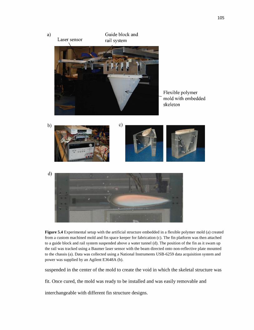
105

Figure 5.4 Experimental setup with the artificial structure embedded in a flexible polymer mold (a) created from a custom machined mold and fin space keeper for fabrication (c). The fin platform was then attached to a guide block and rail system suspended above a water tunnel (d). The position of the fin as it swam up the rail was tracked using a Baumer laser sensor with the beam directed onto non-reflective plate mounted to the chassis (a). Data was collected using a National Instruments USB-6259 data acquisition system and power was supplied by an Agilent E3648A (b).

suspended in the center of the mold to create the void in which the skeletal structure was

fit. Once cured, the mold was ready to be installed and was easily removable and

interchangeable with different fin structure designs.

106

The fin structure, mold, and actuation platform were mounted on a sliding guide

block and rail unit attached to a U-channel aluminum beam. The aluminum beam was

suspended above a Rolling Hills Research Corporation Model 1520-HK Eidetics’ Flow

Visualization Water Tunnel. The rig was suspended over the water tunnel such that only

the over molded portion of the fin was submerged. Since free-swimming simulations

were run in the numerical modeling studies, the test rig was allowed to freely swim up

the rail. The change in position of the rig as it swam up the rail was measured using a

Baumer® laser sensor and the collected data enabled velocity and acceleration

calculations to be made. The total electrical power required to power the rig up the rail

was also monitored through sampling the electrical current between the power source and

Parallax board.

Artificial Structure Experimental Tests

Two artificial fin structures were tested, where each structure was the same with

the exception of the IRJP angle. A structure with a 0-deg IRJP angle structure was tested

as well as a 35-deg IRJP angle structure (Fig 5.5). The 25 degree limit was due to space

constraints where higher angles would lead to an inadequate amount of space between the

axles bolts of connecting segments. Each structure was tested over a narrow range of

prescribed motions, with chord-wise traveling wave number, Nc varied between 0.0 and

0.4. A flapping frequency of 0.75 Hz was selected for each test because ample

acceleration could be achieved at this frequency without inducing excessive loads onto

the system, where the servos would struggle to produce enough torque for good motion

tracking. The two structures were tested for the aforementioned range of motions and

107

were allowed to freely swim up the rail. The velocity data was acquired by taking the

derivative of the time-position data from the Baumer® laser sensor. Second derivative

computations allowed for acceleration values to be calculated which was used in

combination with the measured mass of the test rig and obtain estimates on thrust

production.

Figure 5.5 Artificial fins with different IRJP angles including the baseline artificial fin and modeled counterpart with no IRJP angle (a). This fin was compared to an artificial fin and modeled counterpart with an IRJP angle of 35 degrees (b).

5.2 Results

The experimental results shows that the structure with an increased IRJP angle of

35-degrees accelerated up the rail more quickly than the 0-deg structure which implies

higher thrust production as each structure was attached to the same test rig of the same

mass. The greatest thrust production advantage for the 35-deg over the 0-deg structure

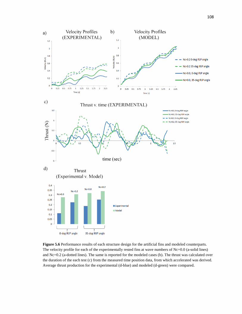
108

Figure 5.6 Performance results of each structure design for the artificial fins and modeled counterparts. The velocity profile for each of the experimentally rested fins at wave numbers of Nc=0.0 (a-solid lines) and Nc=0.2 (a-dotted lines). The same is reported for the modeled cases (b). The thrust was calculated over the duration of the each test (c) from the measured time position data, from which accelerated was derived. Average thrust production for the experimental (d-blue) and modeled (d-green) were compared.

109

was observed for the case in which only flapping motion was prescribed (i.e., no

undulation, Nc = 0.0), in which the 35-deg structure produces approximately 66% more

thrust on average while the fin is accelerating up the rail. At the higher wave number, Nc

= 0.2, the thrust production increase was much less, at approximately 12% on average.

5.3 Discussion

The experimental results show that the IRJP angle leads to gains in thrust

production, which agrees with the modeling results, and further supports the hypothesis

that IRJP angle influences performance. The fin design with an 25-degree IRJP angle was

observed to generate higher thrust than the 0-deg structure, which shows that the skeletal

architecture is not only important for biological fins, but can also be an important design

feature for artificial systems. This is extremely important because it verifies that the

predictions of the model are correct and supports the hypothesis brought forward in

Chapter 2 that the skeletal architecture influences performance.

The results also show that there is a considerable increase in acceleration when

the undulation is increased even slightly from 0.0 to 0.2 waves. Though the modeling

work shows this to be the case also, the increase in thrust production associated with the

transition from 0.0 to 0.2 chord-wise traveling waves, was observed to be much greater in

the experiments than in the modeling. The magnitude of acceleration and velocity were

also higher for the modeled fins than for the experimental fins. This is likely due to a

combination of factors such as friction between the guide block and rail that changes with

110

loading conditions. It is also hypothesized that leading edge separation might be

responsible as increased drag occurs at the onset of flow separation. Since the point at

which flow separation occurs is a function of leading edge angle-of-attack [57,58,59,60],

then it is also a function of leading edge pitch angle, which increases with chord-wise

traveling wave number. Therefore if the change in pitch angle, that follows the addition

of a chord-wise traveling wave, leads to a delay or prevention of leading edge separation,

then this could be the reason behind why a greater disparate in thrust production increases

with increasing wave number is observed in the experiments than in the model, as the

model does not consider leading edge separation. It is also worth discussing the

limitations of using the rail and guide block system as opposed to a fully free swimming

platform. The real rays operate using a pair of fins which are fully submerged and

attached to a body that is also submerged. Therefore the best comparison would be to test

a pair of fins attached to a fully free swimming body that is allowed to translate and

rotate in all directions. The test setup presented in this chapter was vulnerable to the

results being affected by friction between the guide block and rail, as well as any

boundary effects at the point where the fin inserts into the water. The frictional forces

also change through the cycle as both lateral and vertical transient loads are applied to

guide block, leading to an increase in normal force, and therefore frictional force.

Therefore if particular gaits translate to higher normal forces acting on the guide block

than other gaits, that increases the difficulty in making comparisons because one gait

might be burdened by higher rail friction than another. These concerns would be

alleviated, or even eliminated, if a fully free swimming dual fin experimental platform

was used.

111

Despite the differences in thrust values, the performance trends observed for both

the modeling and experimental results are consistent, where both predict increases in

thrust production for fins with a swept-back IRJP. This is a powerful result because both

the computational and experimental tests lead to the same conclusion. They both show

that the underlying skeletal architecture influences performance, and in particular, that

the IRJP angle is related to gains in thrust production. This brings a lot of confidence to

the modeling by reinforcing that the predictions of the model are accurate and further

shows that the model can be used to guide the design of artificial fins to achieve a desired

performance outcome.

112

Chapter 6

Conclusions and future work

Successfully engineering highly functioning AUVs utilizing pectoral-fin-based

propulsion will require contributions from experts in both the physical and life sciences.

Studying the skeletal structure of rays can be an effective route to designing underwater

vehicles [5], however the level of complexity associated with biological systems is often

overwhelming making it difficult or impossible to fully replicate synthetically. Despite

this, principles of the biological system can still be integrated into the design of an

artificial pectoral fin. The objective is to determine which features of the skeletal

structure are most essential to ray swimming performance and for what reason. Once this

foundation has been established, engineers can be selective in choosing which features of

the biological system to leverage in the design of artificial systems. Through

biomechanics, an interface is established between biology and engineering where

computational modeling techniques are used to bridge the gap between biology and

engineering.

Contributions

The present dissertation results in contributions to both biology and engineering.

The knowledge of ray swimming mechanics and associated physiology was further

explained, a link between biology and engineering was established, and the results of this

113

work lead to novel ideas about approaching bio-inspired engineering problems. The

contributions of this work are broken down into components as follows:

1) Explanation of how the actual biological systems of ray pectoral fins function,

and how skeletal architecture influences locomotion

The biomechanical modeling provides insight into ray swimming from a

mechanistic perspective, and further demonstrates that the ray skeletal morphometry is

important in determining the motion that a given ray can achieve. The strain and

displacement analyses discussed in chapter 2 demonstrate that the configuration of the

underlying cartilage structure is an important consideration when it comes to achieving a

desired kinematic profile. This is a contribution to biology as it explains why certain

skeletal patterns appear in some rays and not others. Furthermore, the parameterized

modeling work discussed in chapter 4 shows how each skeletal parameter affects

kinematic performance quantitatively. Reducing the form and function relationships

between skeletal design and performance down to hard metrics, such as the ratio of LE

and TE pitch angle increase with IRJP angle increase, puts the results into a form that not

only provides insight into biology, but can also be used by engineers developing bio-

inspired propulsion systems.

2) Method of integrating a structural model with a CFD model for studying the

fluid-structure-interaction (FSI) of unsteady flow and free-swimming systems

114

The FSI model has not only proven to be a valuable research tool for this work,

but is an approach that could be extended to many other systems as well in which

understanding fluid structure interactions is important. The interface method takes a

structure that is deforming, connects that structure to a surrounding body which interfaces

with a surrounding fluid. As long as the structure involved in the system is defined by a

set of nodes, and if the motion of those nodes can be solved, then the FSI method

introduced in this dissertation can be extended to a wide range of applications. For

example, the propulsive mechanisms of other types of swimming and/or flying organisms

could be modeled, as well the hydrodynamic and/or aerodynamic mechanisms for land

and sea vehicles. Furthermore, when considering the computational efficiency of the

advanced panel code, the utility of this FSI model as a research and analysis tool becomes

even more attractive. The experimental approach can also be extended to be used beyond

the scope of the present dissertation.

3) Quantitative a description of the effect of skeletal design on performance to

inform AUV design

The parameterized modeling discussed in chapter 4 established mathematical

relationships between skeletal design and hydrodynamic performance. In this form, the

metrics can be used by engineers to inform the design of artificial ray-inspired

propulsions systems. For example, the relationship between IRJP angle, LE and TE pitch

angle, and gains in thrust production can provide for a reference on how to achieve a

desired performance outcome. This parameterized modeling also uncovers considerations

such as the development of mechanical strain associated with particular motions.

115

Therefore if a particular performance criterion is desired, that requires a particular

kinematic profile, and the model could be used to find a structure design solution that will

best accommodate the target motion (e.g., required strain levels could be calculated and

materials can be chosen based on the results).

4) Provides design solutions for building and testing artificial structures for

experimental research

It is also important to understand that the successful design and testing of the

experimental rig is alone a contribution as it provides a solution to researching the

physics of ray propulsion experimentally. In the present study, the experimental rig was

only used to conduct a few tests which were used to check the predictions of the

biomechanical fluid structure modeling, and support modeling results. However, the

potential of the test rig is far greater. The level of control and dexterity inherent to the

design would allow for much more extensive and diverse experiments to be run. For

instance, a lot of previous work on bio-inspired underwater propulsion focuses on the

oscillating structures where tests on pitching and heaving airfoils, or flapping flexible

plates, were conducted to learn more about how oscillating propulsion systems function.

However, there is much work that can be done on propulsions systems based more on

undulatory motion. Since the fin design presented in this study allows for a much greater

active control over the fin, tests on undulatory structures with high traveling wave

numbers is well within the limits of the test rig. The system also allows for the level of

undulation in the fin to be controlled independently without being a function of frequency

and amplitude. Previous work has been done on testing the performance of flexible

116

underwater propulsors [refs], where undulation occurs only though passive responsive to

fluid loading. And since fluid loading increases with frequency and amplitude, so does

the fin flexion, and therefore undulation. For these cases studying the effects of

undulation alone is not possible, but is possible, however, for the experimental approach

presented in the present study. Furthermore, the success of the system was the result of

combining the knowledge of ray biomechanics acquired in this study with the knowledge

of artificial pectoral fin design and fabrication introduced by other researchers. It is a

testament to the validity of the biomechanics approach to studying a biological system,

and then using the knowledge gained to drive the design of an artificial biological system,

and should be considered by other scientists and engineers as an appropriate method for

solving other bio-inspired engineering problems.

The tensegrity beam fin actuation platforms proposed by other researchers

[10,12,14]] could benefit from this work as the orientation of the tensegrity structures, or

node staggering between multiple beams (i.e., artificial IRJP), could be informed to

achieve optimal kinematics while keeping strain levels acceptable. The modeling results

also show that an increase in flapping amplitude of the fin tip can be achieved by either

increasing the amplitude of oscillation of each segment (θmax), or by holding the

amplitude of oscillation constant and adding segments onto the radial elements. This

approach can also be applied in cases where an increase in fin tip amplitude is desired,

but the actuators at the fin root are constrained to maximum amplitude of oscillation. The

CT images (Fig. 2.1) suggest that radial elements are made longer through segment

addition as opposed to segment lengthening. From a kinematics perspective, this allows

117

larger amplitude flapping without requiring higher levels of angular deflection (i.e., θmax)

between connecting segments of a single radial element.

Future work

The FSI model in its current state is already an extremely useful tool, but adding

structural dynamics into the modeling process would make the model even more

powerful. Currently, the FSI model just solves for the kinematics of the underlying

structure and the surrounding body, and the structural dynamics are not considered. It is

possible that the reasons behind the differences in skeletal architecture will only present

themselves when the structural dynamics are considered. Modeling the dynamics would

enable things like structural stability and resonance to be included in an analysis. Some

dynamic modeling of batoid fins has been done [62,63], however the fluid models used

are simple and only work on infinitesimally thin representations of a fin, and not 3D fins

with volume. Techniques for incorporating the dynamics into the system are already

being explored at the University of Virginia through the integration of MSC ADAMS

software with MATLAB-Simulink. The ADAMS-MATLAB co-simulation approach has

been done before to treat problems in human biomechanics [63], and a similar approach

is currently being adapted to ray swimming. The technique involves performing inverse

dynamics, where in this case, the fin kinematics and associated fluid reaction forces are

known ahead of time, and the equations of motion are solved to find the applied forces

(in this case input joint torques or muscle forces) that would be required to give rise to

the system kinematics. Computational methods for extracting the input forces from the

CFD simulations, and mapping those forces to the underlying structure have already been

118

added to the fluid-structure code, and is primed for computational dynamics studies to be

conducted.

Incorporating the muscle mechanics into the study is another area for future

work. It was shown that the skeletal architecture is important in determining kinematics

in terms of the fin deformation that can achieved, and that these kinematics differences

affect performance. However, it is also possible that the ray skeletal architecture is

selected to help accommodate optimal muscle function. There has been a lot of work on

muscle mechanics which shows that there are optimal lengths and shortening velocities of

muscle where peaks in force and power occur [65,66,67]. Perhaps the skeletal

architecture is a mechanism for tuning the system such that the optimal fin kinematics

from a hydrodynamics perspective aligns with the kinematics required for optimal muscle

function. For example, if the structure could be designed such that peak hydrodynamic

efficiency occurs at the same kinematic profile as required for optimal muscle shortening

velocity, then gains in efficiency could be realized from both a hydrodynamic and

structural perspective simultaneously. Future work, some of which is already in progress

at West Chester University in Pennsylvania, will involve researching the anatomy and

physiology of ray muscle including among other things, muscle volume measurement and

muscle fiber typing. Once completed, a well-informed muscle model can be incorporated

into the system to address how muscle architecture affects performance.

Expanding on the scope of the experimental tests and refining the

experimental setup is also an area where future can be conducted. The experimental

work was limited to testing just two structures with different IRJP angles. However, the

119

design space of the artificial structures is vast. Not only can IRJP angle be tested on

oscillating fin structures, but undulating fins can be designed and attached to the existing

actuation platform. This would facilitate experimental investigations of other system

parameters, like fanning angle and circular planform, on hydrodynamic performance. The

10 actuator design provides for complete control over the fin motion, and is capable of

reproducing motions with undulatory (Nc) wave numbers of 1.0 or higher, while still

maintaining span-wise curvature. The level of dexterity in the artificial structure design

artificial lends itself to being able to prescribe a wide range of motions, to a wide range of

artificial skeleton designs. There is much room to improve the quality of the

experimentation by adding more instrumentation. For example, including a torque sensor

at the output of each servo would have allowed for direct measurements of the

mechanical power being delivered into the structure. This would allow for fluid-structure

propulsive efficiency calculations to be made in which the mechanical power delivered

into the structure is measured directly and is compared to the propulsive power. Refining

the design of the experimental platform is another area of future work. And when coupled

with the existing capabilities and design foundation, the experimental methods introduced

in this study can be greatly expanded and used to conduct a broad range of tests.

Concluding remarks

The research presented in this dissertation elucidates some of the principles

behind the complexity of pectoral fin designs observed in nature, and puts those

principles in terms that can be used to inform the design of artificial systems for AUV

propulsion. This work establishes an interface between Biology and Engineering will

120

enhance communication between experts with the physical and life sciences. Concepts

from both fields can then be integrating together much more effectively for improving

AUV technology development processes. Furthermore, the proposed research will

demonstrate the viability of adopting a biomechanics approach to analyzing batoid

swimming mechanics and methods for designing batoid inspired artificial fins.

Understanding the function of the real ray skeleton, attached muscle, and controls lays

the foundation for ray inspired AUV design as it provides a base of knowledge that

engineer’s and scientist can access in researching how to design and build next

generation AUVs. The present work demonstrates this idea and shows that the

biomechanics approach is a good one, and that the methods used can be extended beyond

ray inspired technology to benefit any bio-inspired engineering project.

121

References

[1] C.C. Lindsey. Form, function, and locomotory habits in fishes. in fish physiology vol. 7, locomotion (ed. w.s. hoar and d.j. randall). New York: Academic Press, pages 1{100, (1978). [2] P. R. Bandyopadhyay, Trends in biorobotic autonomous undersea vehicles, IEEE Journal of Ocean Engineering 30 (1) (2005) 109–139. [3] C.M. Breder. The locomotion of fishes. Zoologica (n.Y.), 4:159{256, (1926). [4] C. Heine. Mechanics of flapping fin locomotion in the cownose ray, rhinoptera bonasus (elasmobranchii: Myliobatidae). PhD dissertation, Duke University, Durham, NC, USA., (1992). [5] Rosenberger LJ. Pectoral fin locomotion in batoid fishes: undulation versus oscillation. J. Exp. Biol,204:379{394, (2001). [6] Drucker GD Walker JA Westneat MW. Mechanics of pectoral fin swimming in fishes. Fish Physiology, 23:369{423, (2005). [7] Westneat MW Rosenberger LJ. Functional morphology of undulatory pectoral fin locomotion in the stingray, taeniura lymma (chondrichthyes: Dasyatidae). J Exp Biol 202:3523-3539, (1999). [8] JT Schaefer AJ Summers. Batoid wing skeletal structure: Novel morphologies, mechanical implications, and phylogenetic patterns. Journal of Morphology, 264:298{313. doi: 10.1002/jmor.10331, (2005). [9] P.W.Webb. The biology of fish swimming. Mechanics and Physiology of Animal Swimming (ed. L. Maddock, Q. Bone and J.M.V Rayner), Cambridge University Press, pages 45{62, (1994). [10] Moored KW Bart-Smith H. The analysis of tensegrity structures for the design of a morphing wing. J.Appl. Mech. 74, 668 (2007), DOI:10.1115/1.2424718, (2007). [11] Moored KW Fish FE Bart-Smith H. Analytical model to describe pectoral fin kinematics of the mantabirostris: implications for bio-inspired design. TBA, 2010. [12] Moored KW Smith W Hester JM Chang W Bart-Smith H. Investigating the thrust production of myliobatoid-inspired oscillating wing. Advances in Science and Technology, Vol. 58(Mining Smartness from Nature):25{30, (2008). [13] D. Barrett, M. Grosenbaugh, M. Triantafyllou, The optimal control of a flexible hull robotic undersea vehicle propelled by an oscillating foil, Autonomous Underwater

122

Vehicle Technology, 1996. AUV’96.,Proceedings of the 1996 Symposium on (1996) 1–9. [14] A. P. Summers, Stiffening the stingray skeleton an investigation of durophagy in myliobatid stingrays(chondrichthyes, batoidea, myliobatidae), Journal of Morphology 243 (2) (2000) 113–126. [15] R. P. Clark, A. J. Smits, Thrust production and wake structure of a batoid-inspired oscillating fin, Journal of Fluid Mechanics 562 (2006) 415–429. [16] L.J.V. Campagno. Systematics and body form. in sharks, in: Hamlett, w.c. (ed.), skates and rays: The biology of elasmobranch _shes. Johns Hopkins University Press, Baltimore, pages 1{42, (1999). [17] W. Klausewitz. Der lokomotionsmodus der ugelrochen (myliobatoidei). Zool Anz 173:111120, (1964). [18] LJV Campagno. Phyletic relationships of living sharks and rays. Am. Zool., 17:303 { 322, (1977). [19] C.C. Lindsey. Form, function, and locomotory habits in fishes. in fish physiology vol. 7, locomotion (ed. w.s. hoar and d.j. randall). New York: Academic Press, pages 1{100, (1978). [20] J. E. Colgate, K. M. Lynch, Mechanics and control of swimming: a review, Oceanic Engineering, IEEE Journal of 29 (3) (2004) 660–673. [21] M. Fluidic Muscle, Festo Brochure. [22] J. M. Anderson, K. Streitlien, D. S. Barrett, M. S. Triantafyllou, Oscillating foils of high propulsive efficiency, Journal of Fluid Mechanics 360 (1998) 41–72. [23] S. Heathcote, Z. Wang, I. Gursul, Effect of spanwise flexibility on flapping wing propulsion, 36th AIAA Fluid Dynamics Conference and Exhibit. [24] F. E. Fish, G. V. Lauder, Passive and active flow control by swimming fishes and mammals, Ann. Rev. Fluid Mech 38 (2006) 193224. [25] J. E. Colgate, K. M. Lynch, Mechanics and control of swimming: a review, Oceanic Engineering, IEEE Journal of 29 (3) (2004) 660–673. [26] F. Fish L. Howle M. Murray Hydrodynamic flow control in marine mammals, Integr. Comp. Biol. (2008) 48 (6): 788-800. doi: 10.1093/icb/icn029 [27] Moored KW Fish FE Bart-Smith H. Analytical model to describe pectoral fin kinematics of the manta birostris: implications for bio-inspired design. TBA, 2010.

123

[28] Lewin GC Haj-hariri H. Modelling thrust generation of a two-dimensional heaving airfoil in a viscous flow. J. Fluid Mech. (2003), vol. 492, pp 339-362 DOI: 10.1017/S0022112003005743 [29] Wang ZJ. Vortex shedding and frequency selection in flapping flight. J. Fluid Mech. (2000), vol, 410, pp. 323-341 [30] Von Ellenrieder KD Parker K Sorio J. Flow structures behind a heaving and pitching finite-span wing. J. of Fluid Mech. (2003), 490: pp 129-138 DOI: 1017/S0022112003005408 [31] Lewin GC Haj-hariri H. Heaving flapping and its extension to undulatory swimming. American Physical Society, 53rd annual meeting of the vidision of fluid dynamics 19-21, 2000 Washington, DC [32] Perderzani J Haj-hariri H A numerical method for the analysis of flexible bodies in unsteady viscous flows. International Journal for Numerical Methods in Engineering (2006) Vol 68, Issue 10, pp 1096-1112 [33] Tay WB Lim KB Numerical analysis of active chordwise flexibility on performance of non-symmetrical flapping foils. J. of Fluids and Structures, vol 26, issue 1 (2010), pp 74-91 [34] Shin S Yong Bae S Chul Kim I Jig Kim Y Effects of flexibility on propulsive force acting on a heaving foil. J. of Ocean Engineering, vol 36, issues 3-4, (2009), pp 285-294 [35] Zhu Q Kouroush S Propulsion performance of a skeleton-strengthened fin. J. of Experimental Biology 211, (2008), pp 2087-2100 DOI: 10.1242/jeb .016279 [36] Moored KW Kemp TH Houle NE Bart-Smith H. Analytical predictions, optimization, and design of a tensegrity-based artificial pectoral fin. International Journal of Solids and Structures, (2011), vol 48, issues 22-23, pp 3142-3159 [37] Buchholz JHJ Clark RP Smits AJ. Thrust performance of unsteady propulsors using a novel measurement systems, and corresponding wake patterns. Experiments in Fluids, vol 45, pp 461-472 [38] Cai Y Bi S Zheng L. Design and experiments of a robotic fish imitating cow-nosed ray. J. of Bionic Engineering, vol 7, issue 2, (2010), pp 120-126 [39] Dewey PA Carriou A Smits AJ. On the relationship between efficiency and wake structure of a batoid-inspired oscillating fin. J. of Flui Mech (2011), pp 1-22

124

[40] Moored KW Dewey PA Leftwich MC Bart-Smith H Smits AJ. Bioinspired propulsion mechanisms based on manta ray locomotion. Marine Technology Society Journal, (2011), vol 45, pp. 110-118(9) [41] Remus AUV, Woods Hole Oceanic Institute http://www.whoi.edu/page.do?pid=38175 [42] HUGIN AUV, Konsberg Maritime [43] Blue fin Robotics AUVs http://www.bluefinrobotics.com/ [44] Liu J, Dukes I, Hu H. Novel mechtroncis design for robotic fish. Intelligent Robots and Systems (2005) IEEE/RSJ International Conference [45] Low KH. Biomimetic motion planning of an undulating robotic fish fin. J. of Vibration and Control (2006), vol 12 [46] Liu J, Hu H. Mimicry of sharp turning behaviours in a robotic fish. Robotics and Automation (2005). ICRA, pp 3318-3323 DOI: 10.1109/ROBOT.2005.1570622 [47] Chen Z, Shatara S, Tan X. Modeling of biomimetic robotic fish propelled by an ionic polymer-metal composite caudal fin. Mechatronics, IEEE/ASME, vol 15, pp448-459 DOI: 10.1109/TMECH.2009.2027812 [48] McIsaac KA, Ostrowski JP. Motion planning for dynamic eel-like robots. Robotics and Automation (2000), vol 2, pp 1695-1700, DOI: 10.1109/ROBOT.2000.844840 [49] McIsaac KA, Ostrowski JP. Experiments in closed-loop control for an underwater eel-like robot. Robotics and Automation (2002), vol 1, pp 750-755, DOI: 10.1109/ROBOT.2002.1013448 [50] Yu, Junzhi; Hu, Yonghui; Fan, Ruifeng; Wang, Long; Huo, Jiyan. Mechanical design and motion control of a biomimetic robotic dolphin. Advance Robotics, (2007) vol 21, pp 499-513(15) [51] Dogangil G, Ozcicek E, Kuzucu A. Mechatronics and Automation, (2005), Vol 2, pp 952-957, DOI: 10.1109/ICMA.2005.1626680 [52] Moored KW. Analytical model to describe the pectoral fin kinematics of batoid rays: a comparison of swimming performance. TBA [53] L.J.V. Campagno. Systematics and body form in sharks, in: Hamlett, w.c. (ed.), skates and rays: The biology of elasmobranch fishes. Johns Hopkins University Press, Baltimore, pages 1{42, (1999). [54] UC Santa Barbara Masters thesis (Get info)

http://www.whoi.edu/page.do?pid=38175

http://www.bluefinrobotics.com/

125

[55] Han X Yang S, Qiu J. Kinematics modeling and experiments of pectoral oscillation propulsion robotic fish. Journal of Bionic Engineering, 6:174{179, (2009). [56] Calvert RA Comparative anatomy and function morphology of the pectoral fin of stingrays. Dissertation, Department of Zoology, Duke University (1983) [57] Carr LW, McAlister KW, McCroskey WJ. Analysis of the development of dynamic stall based on oscillating airfoil experiments (1977) [58] Vatsa VN, Carter JE. Analysis of airfoil leading-edge separation bubbles, Cost Engineering (1984) [59] Orlov DM, Apker T, He C, Othman H, Corke TC. Modeling and experiment of leading edge separation control using SDBD plasma actuators. The American Institute of Aeronautics and Astronautics (AIAA), (2007) [60] Post ML, Corke TC. Separation control on high angle of attack airfoil using plasma actuators. The American Institute of Aeronautics and Astronautics (AIAA), (2004) [61] Moored KW, Fish FE, Kemp TH. Batoid fishes: Inspiration for the Next Generation of underwater Robots. Marine Technology Society Journal (2011),Vol 45,No.4, pp99-109 [62] Blair JT, Optimal locomotion of mechanical rectifier systems. Dissertation, University of Virginia, 2011 [63] Russell SD, Zirker CA, Blemker SS. A framework for measurement and modeling human climbing. University of Virginia, VA USA [64] Zirker CA, Russell SD, Blemker SS. Variations in climbing strategies between experienced and inexperienced rock climbers. University of Virginia, VA USA [65] Askew GN, Marsh RL. Optimal shortening velocity (V/Vmax) of skeletal muscle during cyclical contractions:length-force effects and velocity-dependent activation and deactivation. Journal of experimental biology (1998) [66] FE Zajac. Muscle and tendon: properties, models, scaling, and application to biomechanics and motor control. Critical reviews in biomedical engineering (1989), 17(4):359-411 [67] Hill AV, The heat of shortening and the dynamic constants of muscle. Proceedings of the Royal Society of London, Series B, (1938)

biomechanical modeling of ray pectoral fins to inform the

Documents