Monte Carlo Integration

Biostatistics 615/815Lecture 22

Reminders

No lecture on Thursday, November 30

Project due on by December 8• Short descriptive report (about 2 pages)• Code and instructions on how to use it

Review session on December 7

Midterm on December 12

Midterm TopicsRandom number generation

Numerical optimization• Golden search• Parabolic interpolation• Nelder Mead simplex method• Simulated annealing• Gibbs sampler

Numerical Integration• Classical methods• Monte-Carlo integration

Last Lecture …

Numerical integration

Classical strategies, with equally spaced abscissas

Discussion of quadrature methods and Monte-Carlo methods

The ProblemEvaluate:

When no analytical solution is readily available

Evaluate f(x) as few times as necessary

Things to consider:• The choice of abscissas• The choice of weights for combining results

dxxfIb

a∫= )(

The Basic Approach

Classical Solutions

Trapezoidal RuleSimpson’s rule

Adaptive integration• Doubled the number of points at each round…

Gaussian quadrature methods• Improved accuracy for smooth functions

Today: Monte Carlo Integration

Basic Monte Carlo Integration

Consider a multidimensional volume V

Consider N random points within V• x1, x2, … xN

Evaluate the function f at each point …

… use observed average to estimate integral

Definitions

The average function value

The average squared function value

Estimate of the integrand (+/- standard error)

Simple Monte Carlo Integration

Sample points within ACalculate proportion π of points in region of interestArea under the curve is the area A π

C Code: Sampling a Point// This code assumes the Random() function returns a// uniformly distributed random number between zero and// one. It then samples a random point within a// multidimensional “rectangular” space.

void SamplePoint(double * point, double * lo, double * hi,int dim)

{for (int i = 0; i < dim; i++)

point[i] = lo[i] + Random() * (hi[i] - lo[i]);}

C Code: Monte Carlo Integraldouble Integrate(double (*f)(double *, int),

double * lo, double * hi, int dim, double N){double * point = alloc_vector(dim);double sum = 0.0, sumsq = 0.0;

for (int i = 0; i < N; i++){SamplePoint(point, lo, hi, dim);

double fx = f(point, dim);sum += fx;sumsq += fx * fx;}

double volume = 1.0;for (int i = 0; i < dim; i++)

volume *= (hi[i] - lo[i]);

free_vector(point, dim);return volume * sum / N;}

Sampling Points

We saw how to sample points from a simple “rectangular” region …

… what if the region of interest as a complicated shape?

Do you have any ideas?

A Complicated Target Region

Numerical Recipes usesthis volume as an exampleof Monte Carlo integration.

The Error Term …

In simple Monte-Carlo integration the error term decreases with

This is not quite as good as with our classic formulas which used equally spaced points…• In those formulas, error is generally proportional to 1/N

N

Challenge

Flexibility of Monte Carlo integration …• Easy to add more points as needed

Efficiency of solutions based on equally spaced points• Accuracy increases faster than

Solution is to sample points “randomly” but also• … “equally spaced”• … avoiding clustering

N

Halton’s Sequence

A quasi-random sequence that fills space

To obtain the jth number in series…• Consider a prime number b• Write j in base b• Reverse the digits of j • Add a leading decimal

In n-dimensions, consider n different primes

Halton’s Sequence (b = 2)

Digits Reversed Base 100 .0 0.0001 .1 0.500

10 .01 0.25011 .11 0.750

100 .001 0.125101 .101 0.625110 .011 0.375111 .111 0.875

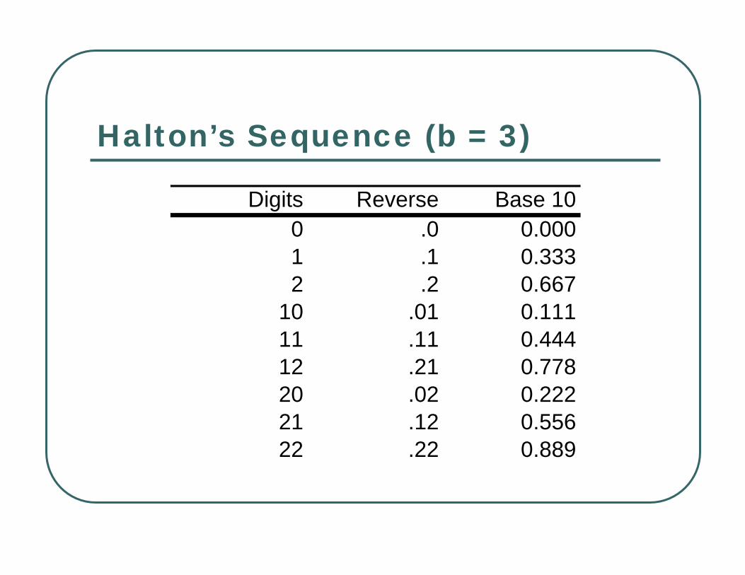
Halton’s Sequence (b = 3)

Digits Reverse Base 100 .0 0.0001 .1 0.3332 .2 0.667

10 .01 0.11111 .11 0.44412 .21 0.77820 .02 0.22221 .12 0.55622 .22 0.889

Sobol’s Sequence

Advantages of Quasi-Random Sequences

Quasi-Random Sequences

Although Halton’s sequence is intuitive, it is a bit cumbersome to code

Other sequences (such as Sobol’s sequence) are more commonly used in practice

They can all greatly improve accuracy of Monte-Carlo integrals

So far …

Random sampling of points is simplest…… but quasi-random sampling is better

Let’s examine why in a bit more detail.

Stratified Sampling, 2 regions

Use random sampling within each one

The estimated average of the function is …

With variance …

Stratified Sampling Improves Accuracy!

Without stratifying, variance would be:

Extra term reflects differences in region specific means

<<>> operator denotes true average

Stratified Sampling, with Different Numbers of Points

In this setting, expected variance of stratified estimate is:

Which is minimized when:

Recursive Stratified Sampling

Given total number of evaluations N

Sample a few points at randomIdentify optimal bisectionIntegrate each half separately• Repeating the steps above in each half that is

not too small…

Practical Nuances

Instead of examining variance in each half• Check minimum and maximum function values

Weights for allocating points are heuristic• Attenuated compared to idealized weights

Should the splits generate equal halves?

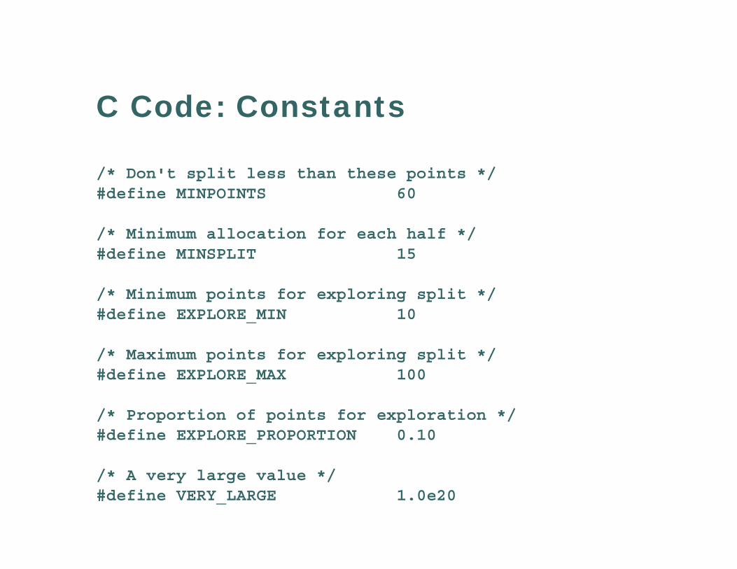
C Code: Constants

/* Don't split less than these points */#define MINPOINTS 60

/* Minimum allocation for each half */#define MINSPLIT 15

/* Minimum points for exploring split */#define EXPLORE_MIN 10

/* Maximum points for exploring split */#define EXPLORE_MAX 100

/* Proportion of points for exploration */#define EXPLORE_PROPORTION 0.10

/* A very large value */#define VERY_LARGE 1.0e20

C Code: Recursive Integration (I)double RecursiveIntegration(double (* f)(double *, int),

double * lo, double * hi, int dim, int N){int RandD; double save, result, totalvar, var0;double * midpoint = alloc_vector(dim);double ** min = alloc_matrix(2, dim);double ** max = alloc_matrix(2, dim);

if (N < MINPOINTS) return Integrate(f, lo, hi, dim, N);

SetupIntegration(lo, hi, midpoint, min, max, dim, N, RandD);ExploreIntegral(f, lo, hi, midpoint, min, max, dim, RandD);int split = ChooseSplit(min, max, dim, totalvar, var0);

int points0 = N * var0 / totalvar;if (points0 < MINSPLIT) points0 = MINSPLIT;

C Code: Recursive Integration (II)save = hi[split]; hi[split] = midpoint[split];result = RecursiveIntegration(f, lo, hi, dim, points0);hi[split] = save;

save = lo[split]; lo[split] = midpoint[split];result += RecursiveIntegration(f, lo, hi, dim, N - points0);lo[split] = save;

free_vector(midpoint, dim);free_matrix(min, 2, dim);free_matrix(max, 2, dim);

return result;}

Helper Functions…The main code delegates nearly all its tasks

SetupIntegration()• Initialize variables • Decide how many points to invest in R&D

ExploreIntegral()• Sample points and collect information for bisection

ChooseSplit()• Decide how best to divide volume

Helper Function Ivoid SetupIntegration(double * lo, double * hi, double * midpoint,

double ** min, double ** max, int dim, int & N, int & RandD){// Calculate midpoint for the current regionfor (int j = 0; j < dim; j++)

{midpoint[j] = 0.5 * (lo[j] + hi[j]);min[0][j] = min[1][j] = VERY_LARGE;max[0][j] = max[1][j] = -VERY_LARGE;}

// Allocate some points to explore the function...RandD = N * EXPLORE_PROPORTION;

if (RandD < EXPLORE_MIN) RandD = EXPLORE_MIN;if (RandD > EXPLORE_MAX) RandD = EXPLORE_MAX;

N -= RandD;}

Helper Function IIvoid ExploreIntegral(double (*f)(double *, int),

double * lo, double * hi, double * midpoint, double ** min, double ** max, int dim, int N)

{double * point = alloc_vector(dim);

for (int n = 0; n < N; n++){SamplePoint(point, lo, hi, dim);double fx = f(point, dim);

for (int j = 0; j < dim; j++){int half = point[j] > midpoint[j];

max[half][j] = fx > max[half][j] ? fx : max[half][j];min[half][j] = fx < min[half][j] ? fx : min[half][j];}

}free_vector(point, dim);}

Helper Function IIIint ChooseSplit(double ** min, double ** max, int dim,

double & var, double & var0){int split = -1;

// Choose the region giving biggest reduction in the variancefor (int j = 0; j < dim; j++)

// have we got two points on each half of the region?if (max[0][j] > min[0][j] && max[1][j] > min[1][j])

{// The lines below use the empirical weightingdouble sigma0 = pow(max[0][j] - min[0][j], 2.0 / 3.0);double sigma1 = pow(max[1][j] - min[1][j], 2.0 / 3.0);

double sigma = sigma0 + sigma1;

if (split == -1 || sigma < var){ split = j; var = sigma; var0 = sigma0; }

}

if (split == -1){ var0 = 1.0; var = 2.0; split = Random() * dim; }

return split;}

Test Results

Integrating a bivariate normal distribution

Simple Monte-Carlo Integration• 100, 1000, 10000, 100000 evaluations• .002, .0006, .0002, .00006 standard error

Recursive stratified sampling• 100, 1000, 10000, 100000 evaluations• .001, .0001, .00001, .000001 standard error

Enhancements

Randomize splits a little bit …

Use Halton’s sequence (or similar) to select points

Today

Monte Carlo Integration• Randomly distributed points

• Points selected to fill space

• Points targeted to high variance regions

The last two strategies can be combined!

Recommended Reading

Numerical Recipes• Chapter 7.6 – 7.8

Available online at:• http://www.nr.com