Biostatistics

Lecture 16 6/8 & 6/9/2015

Ch 15 – Contingency Tables

Outline

• When working with nominal data (or categorical data) that have been grouped into categories, we often arrange the counts in a tabulated format known as contingency tablecontingency table.

• In the simplest case, two dichotomous two dichotomous random variablesrandom variables are involved; the rows of the table represent the outcomes of one variable, and the columns represent the outcomes of the other one.

• A contingency table is often referred as a two-way frequency tabletwo-way frequency table too.

Testing a contingency table• Hypothesis testing can test a table to see

whether a row variable is independent of its column variable.

• H0 assumes that column and row outcomes are independent.

• A test statistic called 2 (read as kai-square, and spelled as Chi-square) is computed, which is a random variable having its own probability density function.

Example #1

• 100 individuals are randomly sampled from a very large population.– Male vs female – Right-handed vs left-handed.

• Here the two dichotomous random variables are “gender” (taking two values “male” and “female”) and “handedness” (taking two values “left-handed” and “right-handed”)

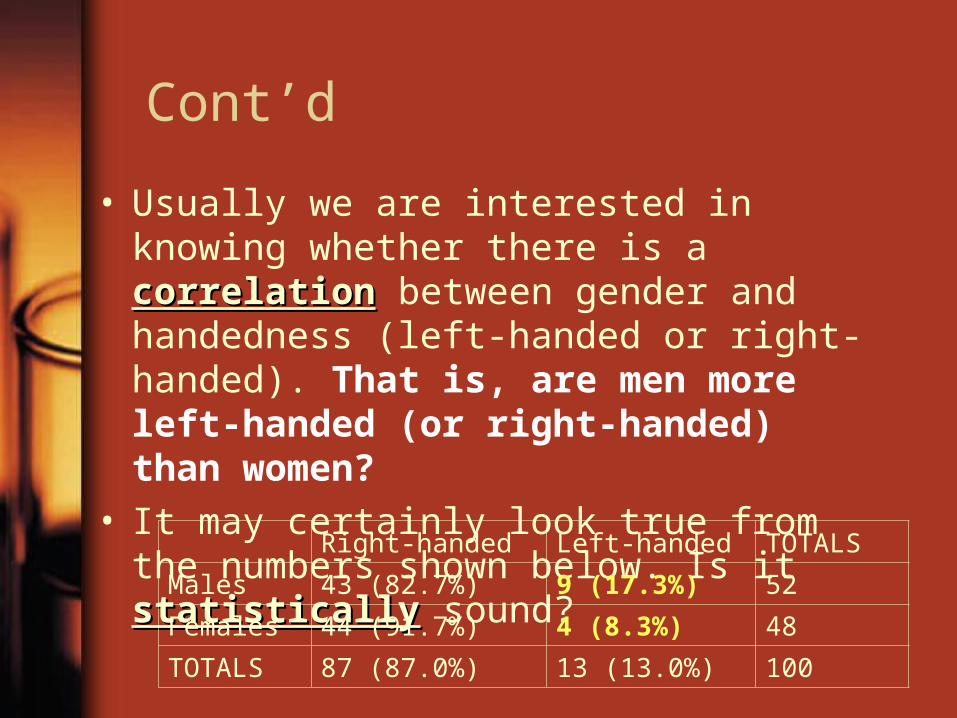
Right-handed Left-handed TOTALS

Males 43 (82.7%) 9 (17.3%) 52Females 44 (91.7%) 4 (8.3%) 48TOTALS 87 (87.0%) 13

(13.0%))100

• We see that the proportion of men who are right-handed (43/52=82.7%) is about about the samethe same as the proportion of women who are right-handed (44/48=91.7%) although the proportions are not identical.

Cont’d

• Usually we are interested in knowing whether there is a correlationcorrelation between gender and handedness (left-handed or right-handed). That is, are men more left-handed (or right-handed) than women?

• It may certainly look true from the numbers shown below. Is it statisticallystatistically sound?

Right-handed Left-handed TOTALS

Males 43 (82.7%) 9 (17.3%) 52

Females 44 (91.7%) 4 (8.3%) 48

TOTALS 87 (87.0%) 13 (13.0%) 100

Cont’d

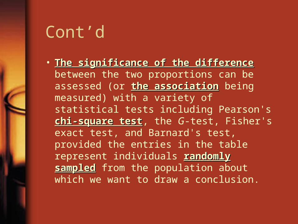
• The significance of the differenceThe significance of the difference between the two proportions can be assessed (or the associationthe association being measured) with a variety of statistical tests including Pearson's chi-square chi-square testtest, the G-test, Fisher's exact test, and Barnard's test, provided the entries in the table represent individuals randomly randomly sampledsampled from the population about which we want to draw a conclusion.

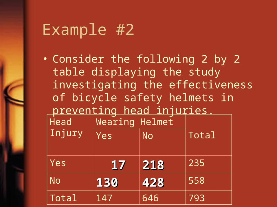
Example #2

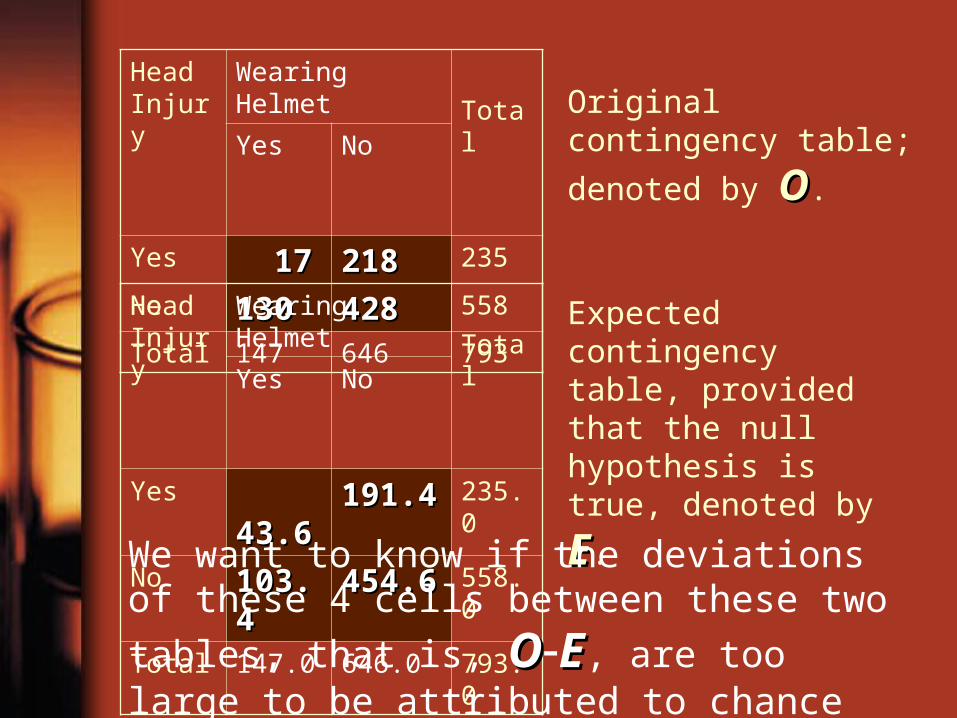
• Consider the following 2 by 2 table displaying the study investigating the effectiveness of bicycle safety helmets in preventing head injuries.

Head Injury

Wearing Helmet

TotalYes No

Yes 1717 218218 235

No 130130 428428 558

Total 147 646 793

Cont’d

• To examine the effectiveness of helmet wearing, we test the null hypothesis at =0.05 level of significance:

– H0: The proportion of persons suffering head injuries for people who wore helmets at the time of accident is the samethe same as the people who did not wear helmet. (有戴與沒戴 , 在意外發生時 , 都一樣會受傷 )

– HA: There is a differencedifference between wearing and not wearing helmet

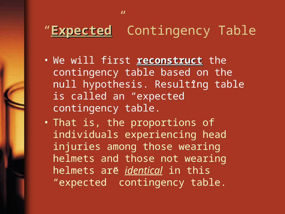
“ExpectedExpected” Contingency Table

• We will first reconstructreconstruct the contingency table based on the null hypothesis. Resulting table is called an “expected” contingency table.

• That is, the proportions of individuals experiencing head injuries among those wearing helmets and those not wearing helmets are identical in this “expected” contingency table.

Head Injury

Wearing Helmet

TotalYes No

Yes 17 218 235 (29.6%29.6%)

No 130 428 558 (70.4%70.4%)

Total 147147 646646 793

We begin by looking at the total column, in which the count of head injury or not is summarized without knowing/concerning whether a helmet was wore or not.

For 793 people, 29.6% had head injury For 793 people, 29.6% had head injury and 70.4% (or the remaining people out and 70.4% (or the remaining people out of the aforementioned 29.6%) did not.of the aforementioned 29.6%) did not.

• Consider the following two groups of individuals now:– For 147 wearing helmetsFor 147 wearing helmets, we’d expect:

• 14729.6%29.6%=43.6 get their heads injured; and 14770.4%70.4%=103.4 not injured.

– For 646 not wearing helmetsFor 646 not wearing helmets, we’d expect:• 64629.6%29.6%=191.4 get their heads injured;

and 64670.4%70.4%=454.6 not injured.

Head Injury Wearing Helmet

TotalYes No

Yes 17 218 235 (29.6%29.6%)

No 130 428 558 (70.4%70.4%)

Total 147147 646646 793

Head Injury

Wearing Helmet

TotalYes No

Yes 1717 218218 235

No 130130 428428 558

Total 147 646 793Head Injury

Wearing Helmet

TotalYes No

Yes 43.643.6 191.4191.4 235.0

No 103.4103.4 454.6454.6 558.0

Total 147.0 646.0 793.0

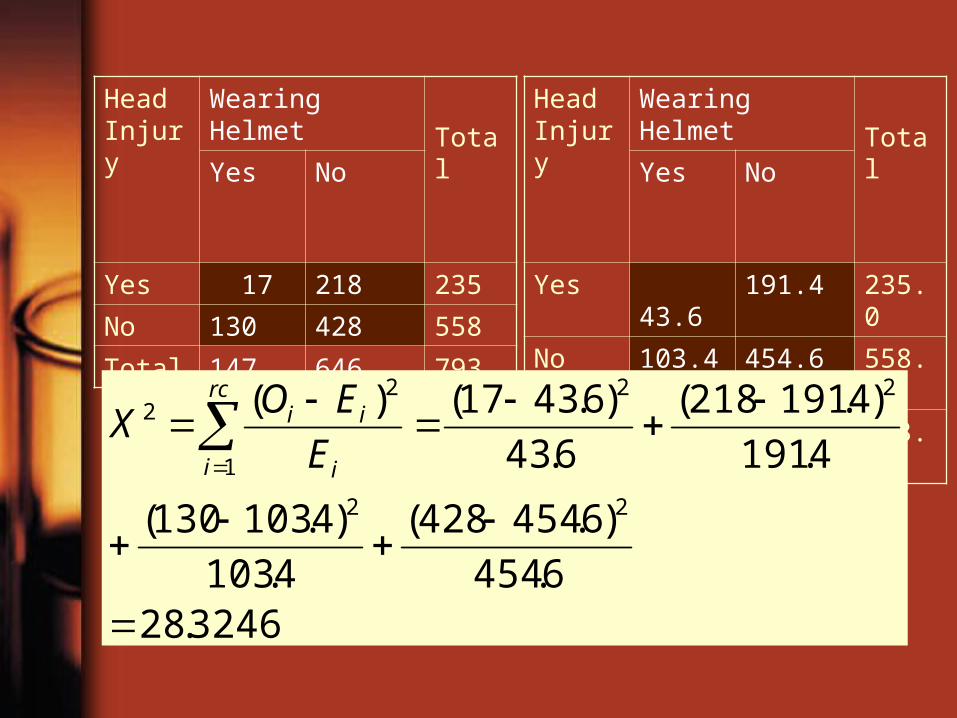
Original contingency

table; denoted by OO.

Expected contingency table, provided that the null hypothesis is true,

denoted by EE.

We want to know if the deviations of these 4

cells between these two tables, that is, OOEE, are too large to be attributed to chance alone.

Chi-Square Test

• The chi-square test compares the observed frequencies (counts) in each category of the contingency table with the expected frequencies given that the null hypothesis is true.

• It is denoted by the following formula, where rc is the number of cells in the table.

rc

i i

ii

E

EOX

1

22 )(

Cont’d

• The probability distribution of this sum is approximated by a chi-square (2) distribution with (r1)(c1) degrees of freedom, with a table of r rows and c columns.

• So a 2 by 2 table will have df= (21)(21)=1, and 3 by 4 table will have df= (31)(41)=6.

• A chi-square distribution is not symmetric.

• The test is The test is one-tailedone-tailed.

>> help chi2pdf chi2pdf CHI2PDF Chi-square probability density function (pdf). Y = CHI2PDF(X,V) returns the chi-square pdf with V degrees of freedom at the values in X.

>> x=0:0.01:20;>> y1=chi2pdf(x,1);>> y6=chi2pdf(x,6);>> plot(x,y1,x,y6)>>

Y1: blue lineY6: green line

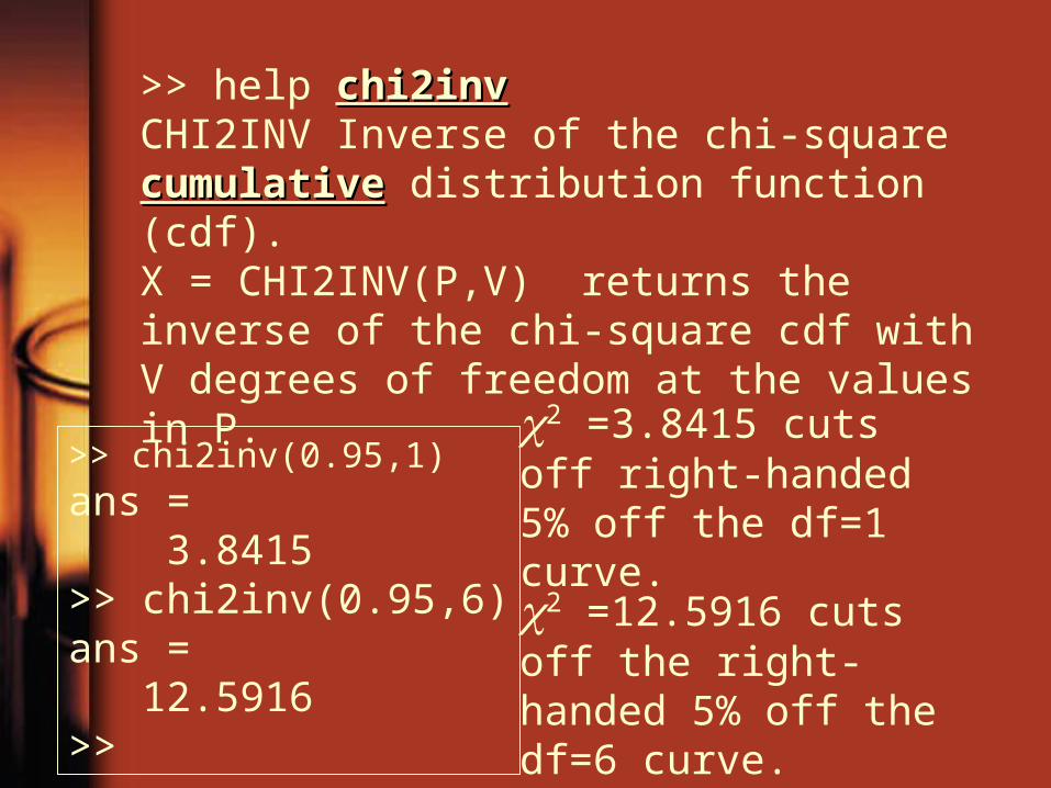
>> help chi2invchi2invCHI2INV Inverse of the chi-square cumulativecumulative distribution function (cdf). X = CHI2INV(P,V) returns the inverse of the chi-square cdf with V degrees of freedom at the values in P.

>> chi2inv(0.95,1)ans = 3.8415>> chi2inv(0.95,6)ans = 12.5916>>

2 =3.8415 cuts off right-handed 5% off the df=1 curve.

2 =12.5916 cuts off the right-handed 5% off the df=6 curve.

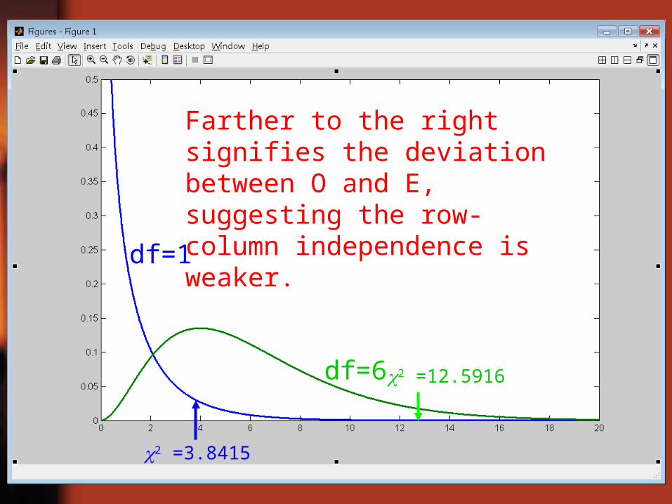
df=1

df=6

2 =3.8415

2 =12.5916

Farther to the right signifies the deviation between O and E, suggesting the row-column independence is weaker.

Head Injury

Wearing Helmet

TotalYes No

Yes 17 218 235

No 130 428 558

Total 147 646 793

Head Injury

Wearing Helmet

TotalYes No

Yes 43.6 191.4 235.0

No 103.4 454.6 558.0

Total 147.0 646.0 793.0

3246.286.454

)6.454428(

4.103

)4.103130(

4.191

)4.191218(

6.43

)6.4317()(

22

22

1

22

rc

i i

ii

E

EOX

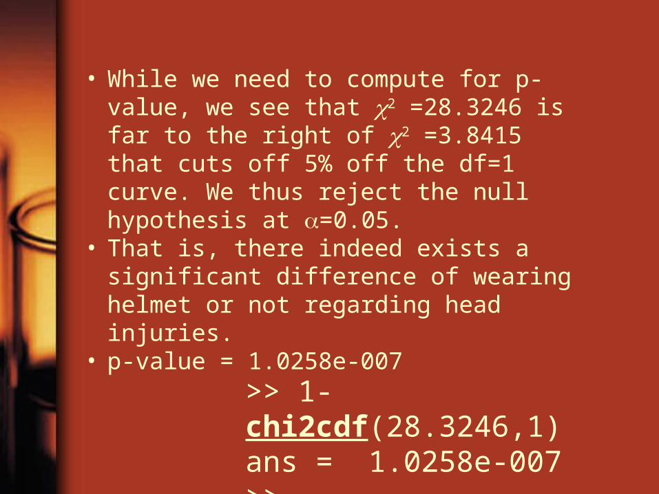
• While we need to compute for p-value, we see that 2 =28.3246 is far to the right of 2 =3.8415 that cuts off 5% off the df=1 curve. We thus reject the null hypothesis at =0.05.

• That is, there indeed exists a significant difference of wearing helmet or not regarding head injuries.

• p-value = 1.0258e-007

>> 1-chi2cdf(28.3246,1)ans = 1.0258e-007>>

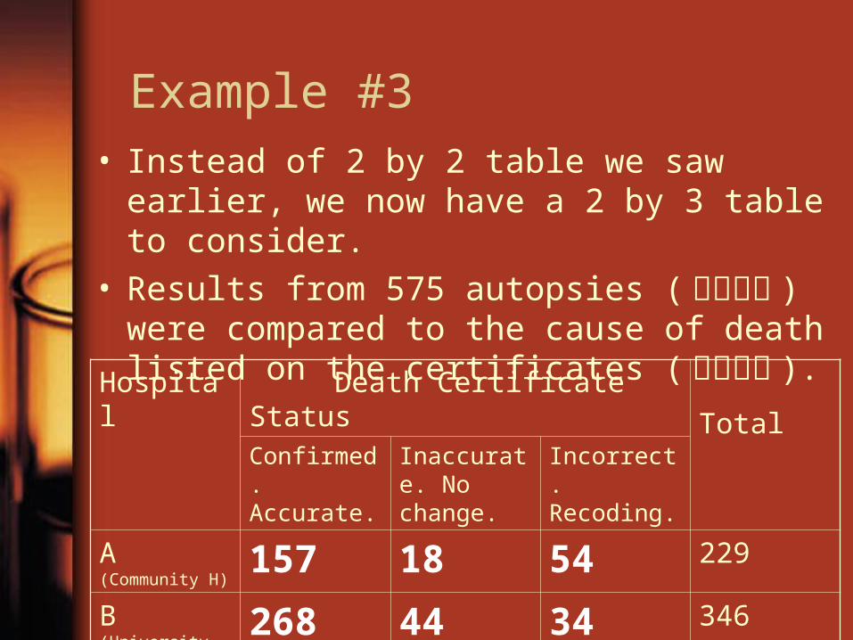
Example #3• Instead of 2 by 2 table we saw earlier, we now

have a 2 by 3 table to consider.• Results from 575 autopsies (解剖驗屍 ) were

compared to the cause of death listed on the certificates (死亡證明 ).

Hospital Death Certificate Status

TotalConfirmed. Accurate.

Inaccurate. No change.

Incorrect. Recoding.

A (Community H)

157 18 54 229

B (University H) 268 44 34 346

Total 425 62 88 575

Cont’d

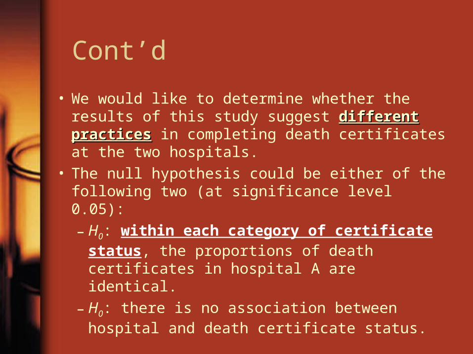
• We would like to determine whether the results of this study suggest different practicesdifferent practices in completing death certificates at the two hospitals.

• The null hypothesis could be either of the following two (at significance level 0.05):

– H0: within each category of certificate status, the proportions of death certificates in hospital A are identical.

– H0: there is no association between hospital and death certificate status.

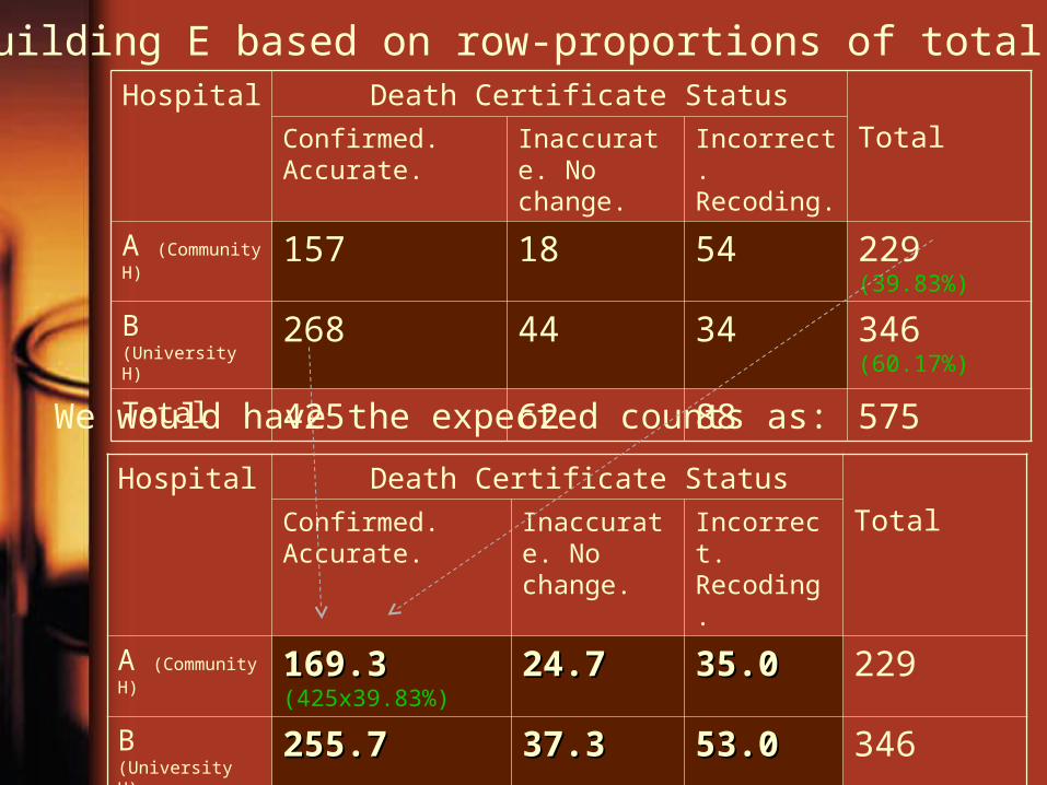
Hospital Death Certificate Status

TotalConfirmed. Accurate.

Inaccurate. No change.

Incorrect. Recoding.

A (Community H)

169.3169.3 (425x39.83%)

24.724.7 35.035.0 229

B (University H) 255.7255.7 37.337.3 53.053.0 346Total 425.0 62.0 88.0 575

We would have the expected counts as:

Hospital Death Certificate Status

TotalConfirmed. Accurate.

Inaccurate. No change.

Incorrect. Recoding.

A (Community H)

157 18 54 229 (39.83%)

B (University H) 268 44 34 346 (60.17%)

Total 425 62 88 575

Building E based on row-proportions of total.

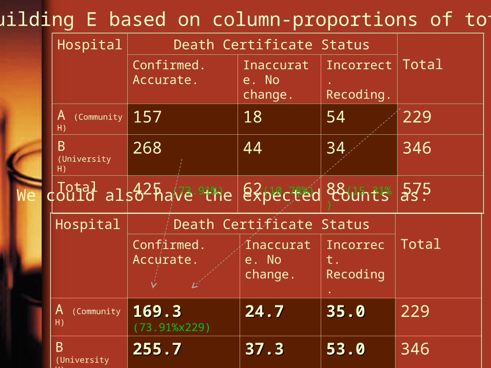
Hospital Death Certificate Status

TotalConfirmed. Accurate.

Inaccurate. No change.

Incorrect. Recoding.

A (Community H)

169.3169.3 (73.91%x229)

24.724.7 35.035.0 229

B (University H) 255.7255.7 37.337.3 53.053.0 346Total 425.0 62.0 88.0 575

We could also have the expected counts as:

Hospital Death Certificate Status

TotalConfirmed. Accurate.

Inaccurate. No change.

Incorrect. Recoding.

A (Community H)

157 18 54 229

B (University H) 268 44 34 346 Total 425 (73.91%) 62(10.78%) 88(15.31%) 575

Building E based on column-proportions of total.

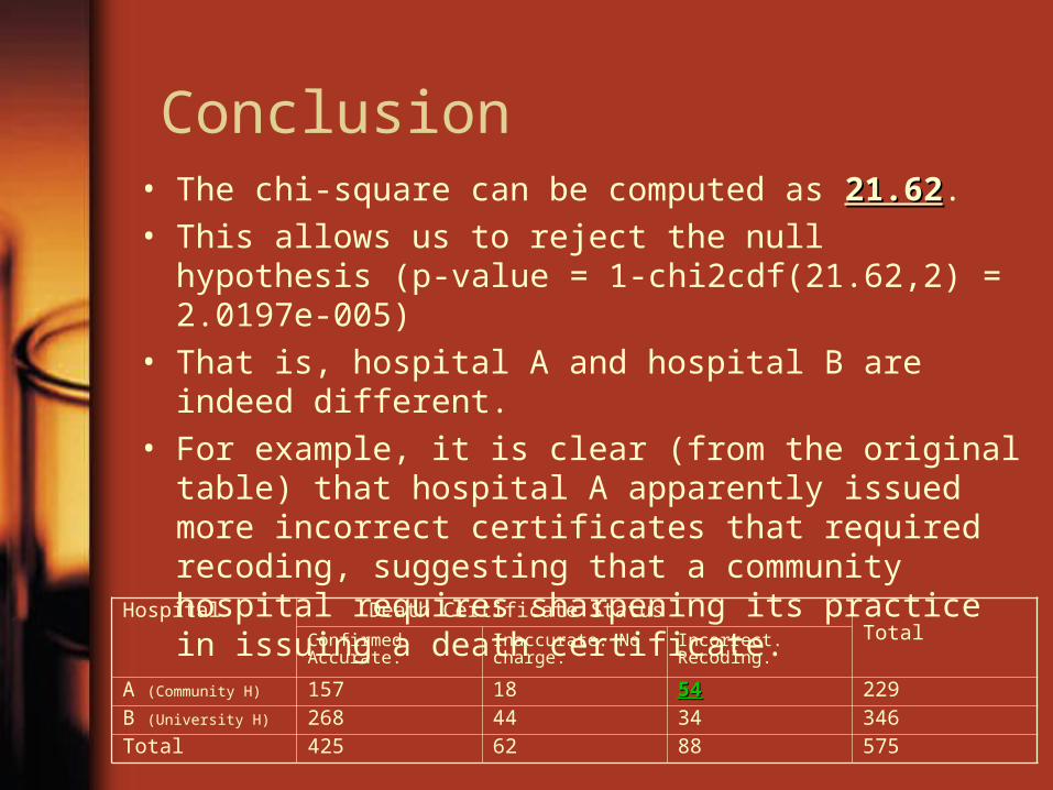
Conclusion• The chi-square can be computed as 21.6221.62. • This allows us to reject the null hypothesis (p-value =

1-chi2cdf(21.62,2) = 2.0197e-005) • That is, hospital A and hospital B are indeed different. • For example, it is clear (from the original table) that

hospital A apparently issued more incorrect certificates that required recoding, suggesting that a community hospital requires sharpening its practice in issuing a death certificate.

Hospital Death Certificate StatusTotalConfirmed.

Accurate.Inaccurate. No charge.

Incorrect. Recoding.

A (Community H) 157 18 5454 229B (University H) 268 44 34 346Total 425 62 88 575

Comments

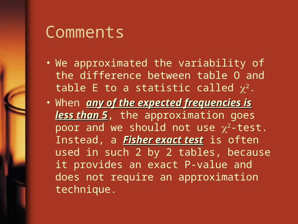
• We approximated the variability of the difference between table O and table E to a statistic called 2.

• When any of the expected frequencies any of the expected frequencies is less than 5is less than 5, the approximation goes poor and we should not use 2-test. Instead, a Fisher exact testFisher exact test is often used in such 2 by 2 tables, because it provides an exact P-value and does not require an approximation technique.

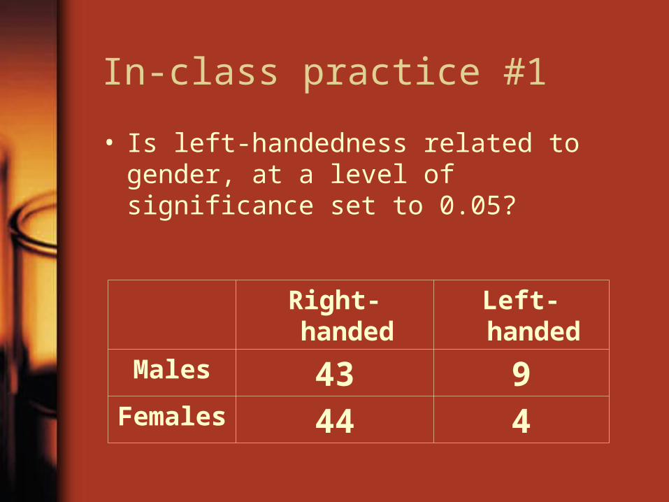
In-class practice #1

• Is left-handedness related to gender, at a level of significance set to 0.05?

Right-handed Left-handed

Males 43 9Females 44 4

Right-handed Left-handed TOTALS

Males 43 (82.7%) 9 (17.3%) 52

Females 44 (91.7%) 4 (8.3%) 48

TOTALS 87 (87.0%) 13 (13.0%)) 100

Right-handed Left-handed TOTALS

Males 52

Females 48

TOTALS 87 (87.0%) 13 (13.0%)) 100

Original table:

Expected table:

Chi-square = ? P-value = ?Conclusion = ?

Right-handed Left-handed TOTALS

Males 43 (82.7%) 9 (17.3%) 52

Females 44 (91.7%) 4 (8.3%) 48

TOTALS 87 (87.0%) 13 (13.0%) 100

Right-handed Left-handed TOTALS

Males E1=87*52/100 E2=13*52/100 52

Females E3=87-E1 E4=13-E2 48

TOTALS 87 (87.0%) 13 (13.0%) 100

Original table:

Expected table:

Chi-square = ? P-value = ?Conclusion = ?

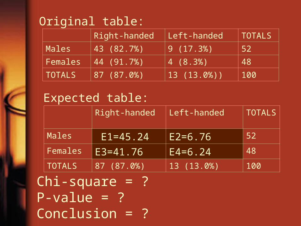
Right-handed Left-handed TOTALS

Males 43 (82.7%) 9 (17.3%) 52

Females 44 (91.7%) 4 (8.3%) 48

TOTALS 87 (87.0%) 13 (13.0%)) 100

Right-handed Left-handed TOTALS

Males E1=45.24 E2=6.76 52

Females E3=41.76 E4=6.24 48

TOTALS 87 (87.0%) 13 (13.0%) 100

Original table:

Expected table:

Chi-square = ? P-value = ?Conclusion = ?

>> O=[43 9 44 4];>> E=[45.24 6.76 41.76 6.24];>> (O-E).^2./Eans = 0.1109 0.7422 0.1202 0.8041>> X2=sum(ans)X2 = 1.77741.7774

>> 1-chi2cdf(X2,1)ans = 0.18250.1825>>

Chi-square statistic = 1.7774. The P-value is 0.1825, which greater than 0.05. We thus did not reject the null hypothesis, which claims no association between gender and handedness.

In-class practice #2

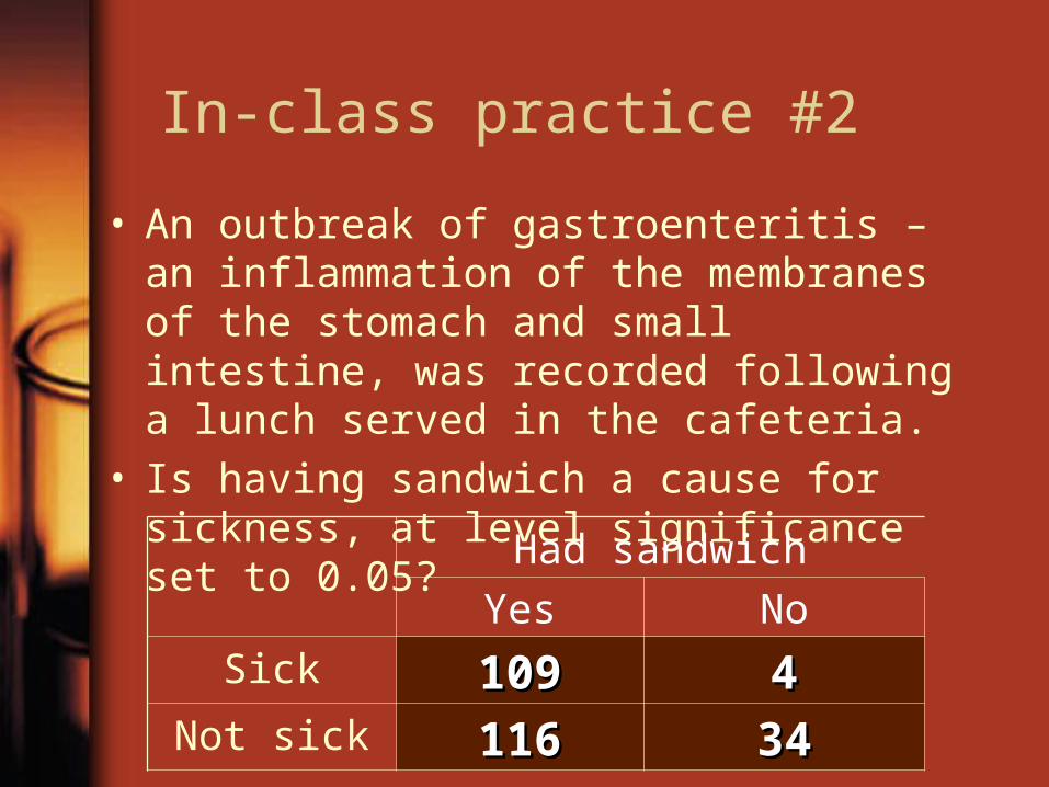
• An outbreak of gastroenteritis – an inflammation of the membranes of the stomach and small intestine, was recorded following a lunch served in the cafeteria.

• Is having sandwich a cause for sickness, at level significance set to 0.05?

Had sandwich

Yes No

Sick 109109 44Not sick 116116 3434

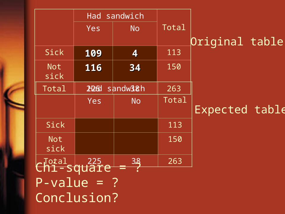
Had sandwich

TotalYes No

Sick 109109 44 113

Not sick 116116 3434 150

Total 225 38 263Had sandwich

TotalYes No

Sick 113

Not sick 150

Total 225 38 263

Original table

Expected table

Chi-square = ? P-value = ?Conclusion?

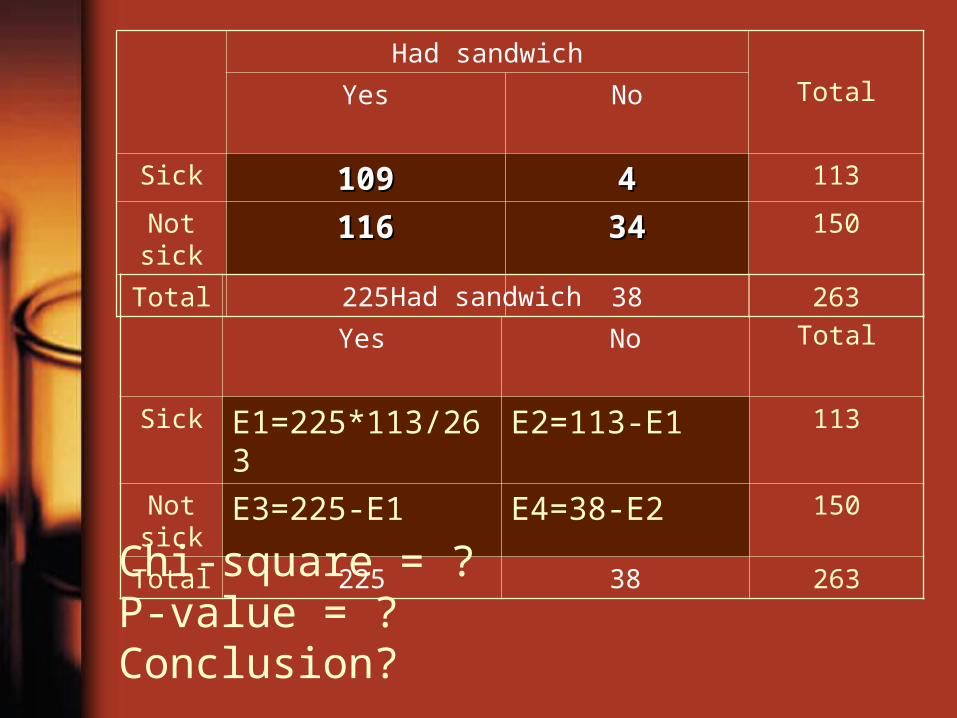
Had sandwich

TotalYes No

Sick 109109 44 113

Not sick

116116 3434 150

Total 225 38 263Had sandwich

TotalYes No

Sick E1=225*113/263 E2=113-E1 113

Not sick

E3=225-E1 E4=38-E2 150

Total 225 38 263Chi-square = ? P-value = ?Conclusion?

Had sandwich

TotalYes No

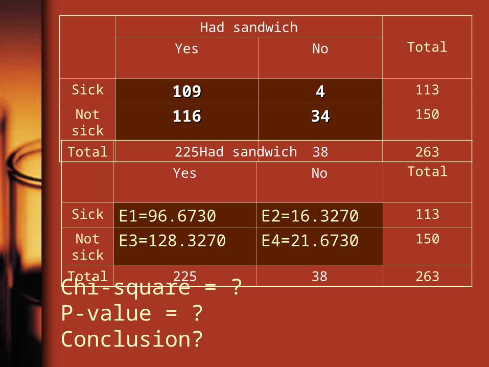
Sick 109109 44 113

Not sick

116116 3434 150

Total 225 38 263Had sandwich

TotalYes No

Sick E1=96.6730 E2=16.3270 113

Not sick

E3=128.3270 E4=21.6730 150

Total 225 38 263Chi-square = ? P-value = ?Conclusion?

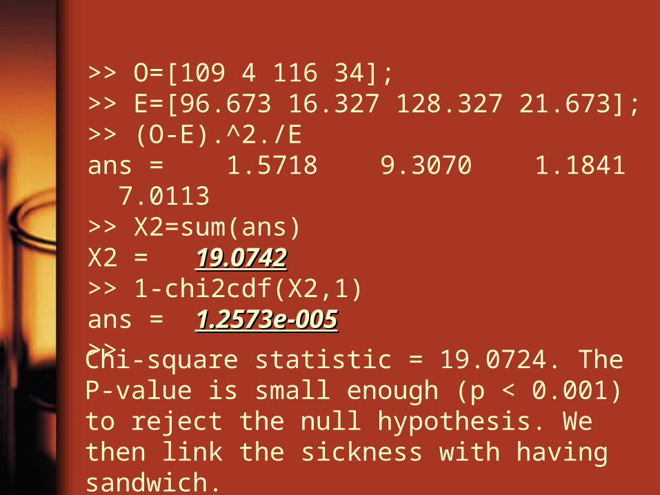
>> O=[109 4 116 34];>> E=[96.673 16.327 128.327 21.673];>> (O-E).^2./Eans = 1.5718 9.3070 1.1841 7.0113>> X2=sum(ans)X2 = 19.074219.0742>> 1-chi2cdf(X2,1)ans = 1.2573e-0051.2573e-005>>

Chi-square statistic = 19.0724. The P-value is small enough (p < 0.001) to reject the null hypothesis. We then link the sickness with having sandwich.