lecture 6: contingency tables continuedpeople.musc.edu/~bandyopd/bmtry711.11/lecture_06.pdf ·...

Lecture 6: Contingency Tables continued

Dipankar Bandyopadhyay, Ph.D.

BMTRY 711: Analysis of Categorical Data Spring 2011

Division of Biostatistics and Epidemiology

Medical University of South Carolina

Lecture 6: Contingency Tables continued – p. 1/59

Recall from previous lecture

• For a contingency table resulting from a prospective study, we derived

Eij =[ith row total] · [jth column total]

[total sample size (n1 + n2) ]

• and the corresponding likelihood ratio test

G2 = 22X

i=1

2X

j=1

Oij log

„Oij

Eij

«

• where Oij is the observed cell count in cell i, j


PEARSON’S CHI-SQUARE

• Another Statistic which is a function of the Oij ’s and Eij ’s is PEARSON’SCHI-SQUARE.

• However, as we will see, Pearson’s Chi-Square is actually just a Z−statistic for testing

H0:p1 = p2 = p versus HA:p1 6= p2 ,

where the standard error is calculated under the null.


• Recall, the WALD statistic is

ZW =(bp1 − bp2) − 0q

n−11 bp1(1 − bp1) + n−1

2 bp2(1 − bp2)

• Note that we used the variance of (bp1 − bp2) calculated under the alternative p1 6= p2.

• Under the null p1 = p2 = p, the variance simplifies to

V ar(bp1 − bp2) =p1(1−p1)

n1+

p2(1−p2)n2

= p(1 − p)h

1n1

+ 1n2

i


• Then, we can use the following test statistic (with the variance estimated under thenull),

ZS =(bp1 − bp2) − 0q

p(1 − p)[n−11 + n−1

2 ]∼ N(0, 1)

where the pooled estimate is used in the variance

p =

„Y1 + Y2

n1 + n2

«


• If we square ZS , we get

X2 = Z2S =

0B@

bp1 − bp2qp(1 − p)[n−1

1 + n−12 ]

1CA

2

∼ χ21

under the null hypothesis.

• After some algebra (i.e., pages), we can write X2 in terms of the Oij ’s and Eij ’s .

• Instead of pages of algebra, how about an empirical proof?


• Consider the following example

Success Failure

Group 1 15 135 150Group 2 10 40 50

Totals 25 175 200

• Herep = (15 + 10)/200 = 0.125

• With SE under the null as

SE0(bp2 − bp1) =q

0.125 ∗ (1 − 0.125) ∗ (150−1 + 50−1) = 0.054006

• Then

Zs =(10/50 − 15/150)

0.054006=

0.1

0.054006= 1.8516402

• andZ2 = 3.428571


Pearson Chi Square

• Likewise, we can use the previous definition of the observed (Oij ) and expected (Eij )to calculate

X2 =2X

i=1

2X

j=1

(Oij − Eij)2

Eij,

which is known as ‘Pearson’s Chi-Square’ for a (2 × 2) table.

• Note, ‘Pearson’s Chi-Square’ measures the discrepancy between the observed counts,and the estimated expected counts under the null; if they are similar, you would expectthe statistic to be small, and the null not to be rejected.


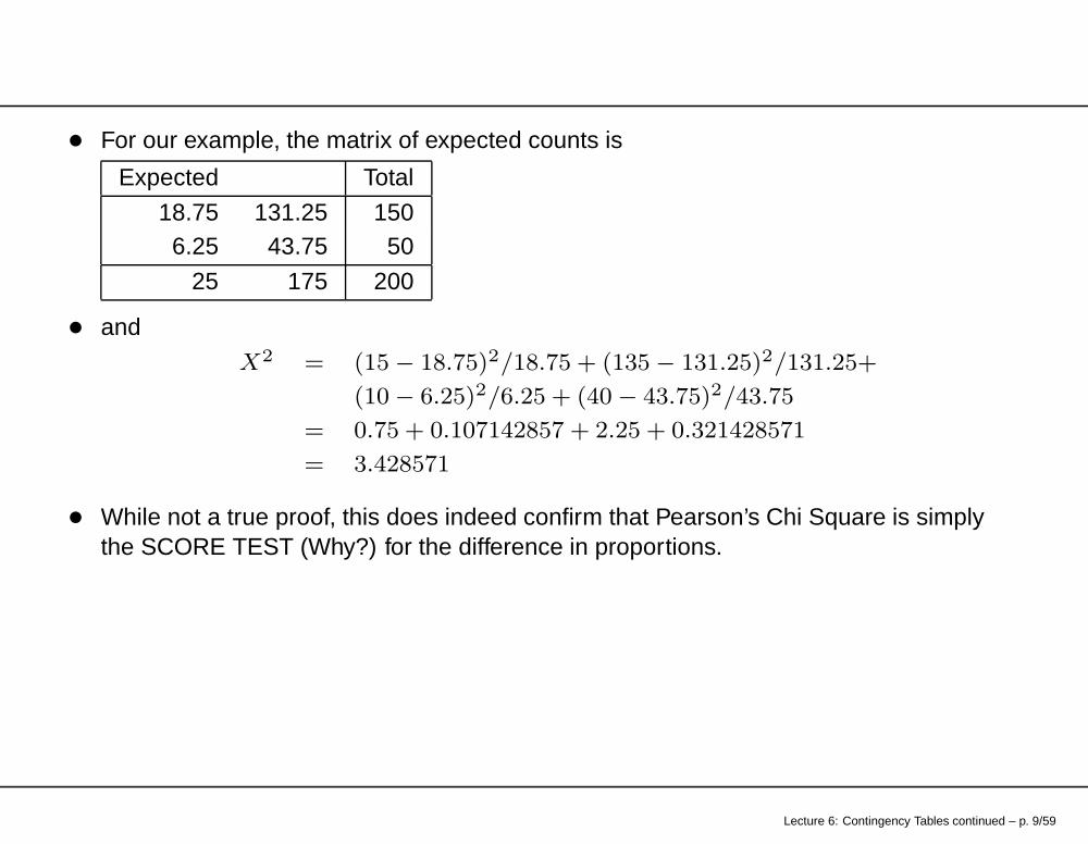
• For our example, the matrix of expected counts is

Expected Total

18.75 131.25 1506.25 43.75 50

25 175 200

• and

X2 = (15 − 18.75)2/18.75 + (135 − 131.25)2/131.25+

(10 − 6.25)2/6.25 + (40 − 43.75)2/43.75

= 0.75 + 0.107142857 + 2.25 + 0.321428571

= 3.428571

• While not a true proof, this does indeed confirm that Pearson’s Chi Square is simplythe SCORE TEST (Why?) for the difference in proportions.


Example using SAS– MI Example

• Recall our MI example from the previous lecture

Myocardial InfarctionFatal Attack or NoNonfatal attack Attack

Placebo 189 10845

Aspirin 104 10933

• We want to investigate whether or not Aspirin is beneficial in the prevention of an MI


Using SAS

Now we can use SAS,data one;input trt $ out $ y;cards;1(P) HA 1891(P) NHA 108452(A) HA 1042(A) NHA 10933;

proc freq;table trt * out / expected chisq measures;weight y; / * tells SAS how many obs. * /

/ * in each cell of 2x2 table * /run;


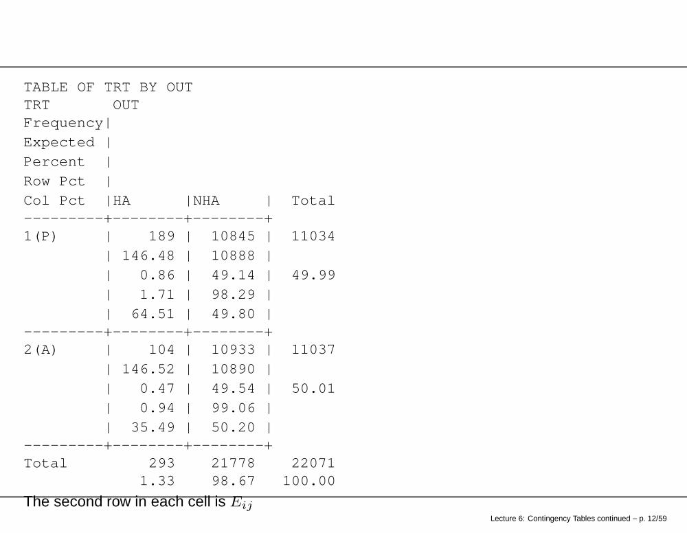
TABLE OF TRT BY OUTTRT OUTFrequency|Expected |Percent |Row Pct |Col Pct |HA |NHA | Total---------+--------+--------+1(P) | 189 | 10845 | 11034

| 146.48 | 10888 || 0.86 | 49.14 | 49.99| 1.71 | 98.29 || 64.51 | 49.80 |

---------+--------+--------+2(A) | 104 | 10933 | 11037

| 146.52 | 10890 || 0.47 | 49.54 | 50.01| 0.94 | 99.06 || 35.49 | 50.20 |

---------+--------+--------+Total 293 21778 22071

1.33 98.67 100.00

The second row in each cell is EijLecture 6: Contingency Tables continued – p. 12/59

Estimated Expected Cell Counts

• If you work thru the (2 × 2) table, you will see

E11 = 146.48

=[1st row total] · [1st column total]


=(11034)(293)

22071

E12 = 10888

=[1st row total] · [2nd column total]


=(11034)(21778)

22071


E21 = 146.52

=[2nd row total] · [1st column total]


=(11037)(293)

22071

and

E21 = 10890

=[2nd row total] · [2nd column total]


=(11037)(21778)

22071


More SAS PROC FREQ OUTPUT

STATISTICS FOR TABLE OF TRT BY OUT

Statistic DF Value Prob--------------------------------------------------- ---Chi-Square 1 25.014 0.000<=(Pearson’s,Score)Likelihood Ratio Chi-Square 1 25.372 0.000<=LR STATContinuity Adj. Chi-Square 1 24.429 0.000Mantel-Haenszel Chi-Square 1 25.013 0.000Fisher’s Exact Test (Left) 1.000

(Right) 3.25E-07(2-Tail) 5.03E-07

Phi Coefficient 0.034Contingency Coefficient 0.034Cramer’s V 0.034


Estimates of the Relative Risk (Row1/Row2)

95%Type of Study Value Confidence Bounds--------------------------------------------------- --Case-Control 1.832 1.440 2.331 <=(OR, using logOR)Cohort (Col1 Risk) 1.818 1.433 2.306 <=(RR, using logRR)Cohort (Col2 Risk) 0.992 0.989 0.995

Sample Size = 22071


Comparing Test Statistics

• We want to compare test statistics for

H0:p1 = p2 = p versus HA:p1 6= p2

• Recall our results from the previous lecture,

Estimated Z−StatisticParameter Estimate Standard Error (Est/SE)

RISK DIFF .0077 .00154 5.00

log(RR) .598 .1212 4.934(RR=1.818)

log(OR) .605 .1228 4.927(OR=1.832)


• Looking at the (square of the) WALD statistics from earlier, as well as the LikelihoodRatio and Pearson’s Chi-Square calculated by SAS, we have

STATISTIC VALUE

WALD

RISK DIFF 25.00

log(RR) 24.34

log(OR) 24.28

LR 25.37

Pearson’s 25.01


• We see that all of the statistics are almost identical. We would reject the null using anyof them (the .05 quantile is 3.84 = 1.962.

• All of the test statistics are approximately χ21 under the null, and are actually equivalent

at n1 = ∞ and n2 = ∞.

• Under a given alternative, all will have high power (although not exactly identical).

• Note, the likelihood ratio and Pearson’s Chi-Square statistic just depend on thepredicted probabilities (i.e., the ‘Estimated Expected Cell Counts’). and not how wemeasure the treatment difference.

• However, the WALD statistic does depend on what treatment difference (RiskDifference, log OR, or log RR) we use in the test statistic.

• In other words, the WALD test statistics using the Risk Difference, log OR, and log RRwill usually be slightly different (as we see in the example).


Empirical Logits

• Recall, we can write the estimated log-odds ratio as

logdOR = log“

bp11−bp1

”− log

“bp2

1−bp2

”

= log“

y1/n1(n1−y1)/n1

”− log

“y2/n2

(n2−y2)/n2

”

= log“

y1n1−y1

”− log

“y2

n2−y2

”

= log(y1) − log(n1 − y1)

− log(y2) + log(n2 − y2)

• Question: What happens if y1 = 0, or y1 = n1, (n1 − y1 = 0) or y2 = 0, or y2 = n2,

(n2 − y2 = 0), so that logdOR is indeterminate ?

• How will you adjust?


• Instead of „yt

nt − yt

«

use „yt + a

(nt − yt) + a

«

where the constant a > 0 is chosen so that, as nearly as possible,

E

„yt + a

(nt − yt) + a

«=

pt

1 − pt


• Haldane (1956) showed by a first order Taylor Series approximation,

a = .5

• The quantity

log

„yt + .5

(nt − yt) + .5

«

is called an “empirical logit",

• The “empirical logit" has smaller finite sample bias than the usual logit.


• Using empirical logits is like adding .5 to each cell of the (2 × 2) table, and get

dORE

=(Y1 + .5)(n2 − Y2 + .5)

(Y2 + .5)(n1 − Y2 + .5)

and

dV ar{log[dORE

]} =1

y1 + .5+

1

n1 − y1 + .5+

1

y2 + .5+

1

n2 − y2 + .5

• The empirical logit was used more before exact computer methods became available(we will discuss these later).

• Not always liked because, some investigators feel that you are adding ‘fake’ data, eventhough, it does have smaller finite sample bias, and, is asymptotically the same as theusual estimate of the log odds ratio.


Case-Control Studies

Lecture 06 - Part B


Probability Structure for a Case-Control Study

• Alcohol Consumption and occurrence of esophageal cancer (Tuyms et al., Bulletin ofCancer, 1974)

• It is not ethical to randomize patients in a prospective study

STATUS

|CASE |CONTROL | TotalA ---------+--------+--------+L 80+ | | |C (gm/day) | 96 | 109 | 205O | | |H ---------+--------+--------+O 0-79 | | |L (gm/day) | 104 | 666 | 770

| | |---------+--------+--------+Total 200 775 975

ˆ ˆ| |----------(fixed by design)


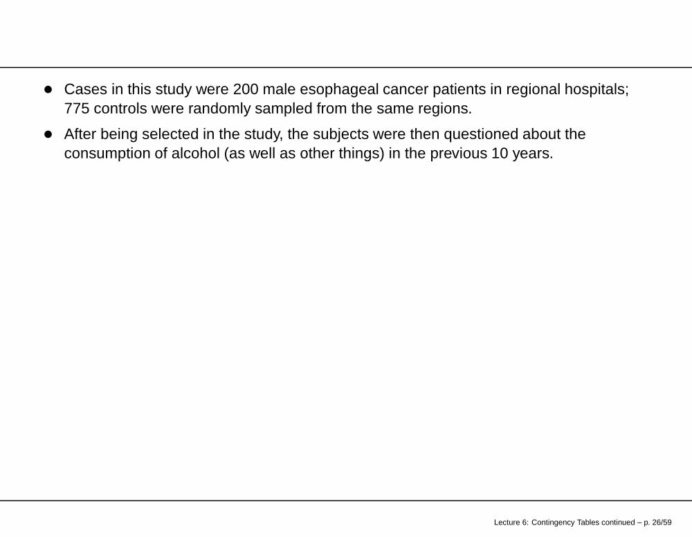
• Cases in this study were 200 male esophageal cancer patients in regional hospitals;775 controls were randomly sampled from the same regions.

• After being selected in the study, the subjects were then questioned about theconsumption of alcohol (as well as other things) in the previous 10 years.


Case-Control Design

• Number of cases and controls (usually the outcomes) are fixed by design andexposures are random.

• Columns are independent binomials.

• Question of interest:Does alcohol exposure vary among cases and controls?Is alcohol exposure associated with esophageal cancer?


Comparison to Prospective Design

• Suppose you use SAS as if the data were a prospective study.

• Would your analyses be OK ?

data one;input exp $ ca $ count;cards;1 1 961 2 1092 1 1042 2 666;

proc freq;table exp * ca / expected chisq measures;weight count; / * tells SAS how many obs. * /

/ * in each cell of 2x2 table * /run;


Selected Results

EXP CAFrequency|Expected |Percent |Row Pct |Col Pct |1 |2 | Total---------+--------+--------+1 | 96 | 109 | 205

| 42.051 | 162.95 || 9.85 | 11.18 | 21.03| 46.83 | 53.17 || 48.00 | 14.06 |

---------+--------+--------+2 | 104 | 666 | 770

| 157.95 | 612.05 || 10.67 | 68.31 | 78.97| 13.51 | 86.49 || 52.00 | 85.94 |

---------+--------+--------+Total 200 775 975

20.51 79.49 100.00


STATISTICS FOR TABLE OF EXP BY CA

Statistic DF Value Prob--------------------------------------------------- ---Chi-Square 1 110.255 0.000 (Pearson’s)Likelihood Ratio Chi-Square 1 96.433 0.000 (Gˆ2)Continuity Adj. Chi-Square 1 108.221 0.000Mantel-Haenszel Chi-Square 1 110.142 0.000Fisher’s Exact Test (Left) 1.000

(Right) 1.03E-22(2-Tail) 1.08E-22

Phi Coefficient 0.336Contingency Coefficient 0.319Cramer’s V 0.336

Estimates of the Relative Risk (Row1/Row2)95%

Type of Study Value Confidence Bounds--------------------------------------------------- ---Case-Control 5.640 4.001 7.951 (OR)Cohort (Col1 Risk) 3.467 2.753 4.367Cohort (Col2 Risk) 0.615 0.539 0.701


General Case Control Study

• Disease Status is known and fixed in advance:

• First, you go to a hospital and get patients with lung cancer (case) and patients withoutlung cancer (control)

• Conditional on CASE/CONTROL status, exposure is the response:Go back in time to find exposure, i.e., smoked (exposed) and didn’t smoke(unexposed).


Summary Counts

DISEASE STATUSCase Control

YESEXPOSED

NO

Y1 Y2

n1 − Y1 n2 − Y2

n1 n2


Setting is similar to a prospective study

• n1 and n2 (columns) are fixed by design

• Y1 and Y2 are independent with distributions:

Y1 ∼ Bin(n1, π1) and Y2 ∼ Bin(n2, π2)

where

π1 = P [Exposed|Case] and π2 = P [Exposed|Control]

• The (2 × 2) table of probabilities are

DISEASE1 2 total

1 π1 π2 (π1 + π2)

EXPOSE2 (1 − π1) (1 − π2) [2 − (π1 + π2)]

total 1 1 2


• In a case-control study, π1, π2 and any parameters that can be expressed as functionsof π1 and π2 can be estimated.

• However, the quantities of interest are not π1, π2 but, instead, are

p1 = P [Case|Exposed] and p2 = P [Case|Unexposed],

in the (2 × 2) table:

DISEASE1 2

1 p1 (1 − p1) 1EXPOSE

2 p2 (1 − p2) 1

• In the CASE-CONTROL study, we want to know:Does exposure affect the risk of (subsequent) disease ?

• Problem: p1 and p2 cannot be estimated from this type of design (i.e., neither can beexpressed as functions of the quantities which can be estimated, π1 and π2).


• Since we are allowed to choose the number of cases and controls in the study, wecould just as easily have chosen 775 cases and 200 controls.

• Thus, the proportion of cases is chosen by design, and could have nothing to do withthe real world. Esophageal cancer is a rare disease. There is no way that theprobability of Esophageal cancer in the population is

bP [Case] =200

975= .205

• Further, the estimates

bp1 = bP [Case|Exposed] =96

205= .47

and

bp2 = bP [Case|Unexposed] =104

770= .14

are not even close to what they are in the real world.

• Bottom line: cannot estimate p1 and p2 with case-control data.


ODDS RATIO

• However, we will now show that, even though p1 and p2 can not be estimated, the“odds ratio” as if the study were prospective, can be estimated from a case-controlstudy, i.e., we can estimate

OR =p1/(1 − p1)

p2/(1 − p2)=

p1(1 − p2)

p2(1 − p1)

• We will use Baye’s Rule to show that you can estimate the OR from a case-controlstudy. Baye’s rule states that

P [A|B] =P [AB]

P [B]=

P [B|A]P [A]

P [B]

=P [B|A]P [A]

P [B|A]P [A] + P [B|not A]P [not A]


• For example, applying Baye’s rule to

p1 = P [Case|Exposed],

we get

p1 = P [Case|Exposed]

=P [Exposed|Case]P [Case]

P [Exposed]

= π1

„P [Case]

P [Exposed]

«,

where, recall

π1 = P [Exposed|Case]

• By applying Baye’s rule to each of the probabilities in the odds ratio for a prospectivestudy, p1, (1 − p1), p2 and (1 − p2), you can show that


The odds ratio for a prospective study equals

p1/(1−p1)p2/(1−p2)

=

“π1π2

”»P [Case]

P [Control]

–

“1−π11−π2

”»P [Case]

P [Control]

–

=π1/(1−π1)π2/(1−π2)

= OR from case-control (2 × 2) table

whereπ1/(1 − π1)

is the “odds” of being exposed given a case, and

π2/(1 − π2)

is the “odds” of being exposed given a control.


Thus, we can estimate

OR =p1/(1 − p1)

p2/(1 − p2)

with an estimate of

OR =π1/(1 − π1)

π2/(1 − π2)

since the OR can be equivalently defined in terms of the p’s or the π’s.


Proof

Using Baye’s Rule, first, let’s rewrite

p1

1 − p1=

P [Case|Exposed]

P [Control|Exposed]

Now,

p1 = P [Case|Exposed]

=P [Exposed|Case]P [Case]

P [Exposed]

= π1

“P [Case]

P [Exposed]

”

and

1 − p1 = P [Control|Exposed]

=P [Exposed|Control]P [Control]

P [Exposed]

= π2

“P [Control]

P [Exposed]

”


Then

p11−p1

=“

π1π2

”»P [Case]/P [Exposed]

P [Control]/P [Exposed]

–

=“

π1π2

” hP [Case]

P [Control]

i

Similarly, you can show that

p21−p2

=“

1−π11−π2

”»P [Case]/P [Unexposed]

P [Control]/P [Unexposed]

–

=“

1−π11−π2

” hP [Case]

P [Control]

i


Then, the odds ratio is

p1/(1−p1)p2/(1−p2)

=

“π1π2

”»P [Case]

P [Control]

–

“1−π11−π2

”»P [Case]

P [Control]

–

=π1/(1−π1)π2/(1−π2)

= OR from case-control (2 × 2) table,

whereπ1/(1 − π1)

is the “odds” of being exposed given a case, and

π2/(1 − π2)

is the “odds” of being exposed given a control.


Notes

• OR in terms of (p1, p2) is the same as OR in terms of (π1, π2)

• OR, which measures how much p1 and p2 differ, can be estimated from a case-controlstudy, even though p1 and p2 cannot.

• We can make inferences about OR, without being able to estimate p1 and p2.

• If we have additional information on P [Case] or P [Exposed], then we can estimate p1

and p2.

• Then for a case-control study, we usually are only interested in estimating the OR andtesting if it equals some specified value (usually 1).


Estimates

The likelihood is again product binomial (the 2 columns are independent binomials):

L(π1, π2) = P (Y1 = y1|π1)P (Y2 = y2|π2)

=

n1

y1

! n2

y2

!πy11 (1 − π1)n1−y1πy2

2 (1 − π2)n2−y2


Question of interest

Are exposure and case control status associated?

Estimating the OR to look at this association is of the most interest, but to estimate the

OR =π1/(1 − π1)

π2/(1 − π2),

we must first estimateπ1 = P [Exposed|Case]

andπ2 = P [Exposed|Control]


• Going thru the same likelihood theory as we did for estimating (p1, p2) from twoindependent binomials in a prospective study, the MLE’s of (π1, π2) are theproportions exposed given case and control, respectively,

bπ1 =Y1

n1and bπ2 =

Y2

n2

• Then,

dOR =bπ1/(1 − bπ1)

bπ2/(1 − bπ2)

=(y1/n1)/[1 − (y1/n1)]

(y2/n2)/[1 − (y2/n2)]

=y1(n2 − y2)

y2(n1 − y1)


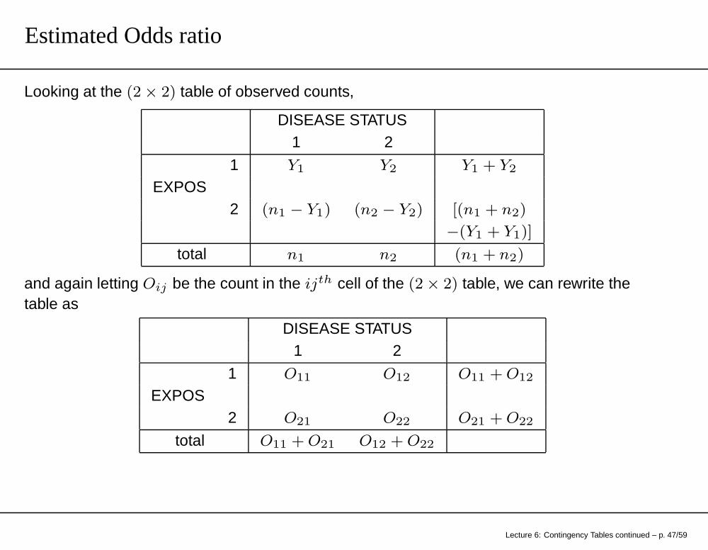
Estimated Odds ratio

Looking at the (2 × 2) table of observed counts,

DISEASE STATUS1 2

1 Y1 Y2 Y1 + Y2

EXPOS2 (n1 − Y1) (n2 − Y2) [(n1 + n2)

−(Y1 + Y1)]

total n1 n2 (n1 + n2)

and again letting Oij be the count in the ijth cell of the (2 × 2) table, we can rewrite thetable as

DISEASE STATUS1 2

1 O11 O12 O11 + O12

EXPOS2 O21 O22 O21 + O22

total O11 + O21 O12 + O22


The estimated odds ratio equals

dOR =y1(n2 − y2)

y2(n1 − y1)

=O11O22

O12O21,

which is the same thing we would get if we treated the case-control data as if it wasprospective data.


Testing

The null hypothesis of no association is or, usually,

H0:OR = 1

and the alternative isHA:OR 6= 1

Where,

dOR =y1(n2 − y2)

y2(n1 − y1)=

O11O22

O12O21,

(which is the same as if the study was a prospective study.)


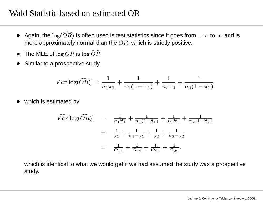
Wald Statistic based on estimated OR

• Again, the log(dOR) is often used is test statistics since it goes from −∞ to ∞ and ismore approximately normal than the OR, which is strictly positive.

• The MLE of log OR is logdOR

• Similar to a prospective study,

V ar[log(dOR)] =1

n1π1+

1

n1(1 − π1)+

1

n2π2+

1

n2(1 − π2)

• which is estimated by

dV ar[log(dOR)] = 1n1bπ1

+ 1n1(1−bπ1)

+ 1n2bπ2

+ 1n2(1−bπ2)

= 1y1

+ 1n1−y1

+ 1y2

+ 1n2−y2

= 1O11

+ 1O12

+ 1O21

+ 1O22

,

which is identical to what we would get if we had assumed the study was a prospectivestudy.


• The WALD statistic for H0 : OR = 1, i.e.,H0 : log(OR) = 0, is

Z =log(dOR) − 0qdV ar(log(dOR))

,

• Also, a 95% confidence interval for the odds ratio is

exp{log(dOR) ± 1.96

qdV ar[log(dOR)]}

• The bottom line here is that you could treat case-control data as if it came from aprospective study and get the same test statistic and confidence interval describedhere.


Cross-sectional Studies

Lecture 06 - Part C


Double Dichotomy or Cross-sectional

Job SatisfactionDissatisfied Satisfied

Income < $15, 000 104 391 495≥ $15, 000 66 340 406

170 731 901

• Neither margin is fixed by design, although the total sample size n (901) is fixed

• Study Design–Randomly select n (fixed) independent subjects and classify each subjecton 2 variables, say X and Y, each with two levels

• For example,

X = Income =

(1 if < $15, 000

2 if ≥ $15, 000

Y = JOB SATISFACTION =

(1 if Not Satisfied2 if Satisfied


Question of interest

• Are X and Y associated or are they independent ?

• Under independence,

P [(X = i), (Y = j)] = P [X = i] · P [Y = j],

i.e.,

pij = pi·p·j

• Then, the null hypothesis is

H0:pij = pi·p·j for i, j = 1, 2.

and the alternative isHA:pij 6= pi·p·j


Parameters of interest

• We are interested in the association between X and Y.

• We may ask: Are X and Y independent ?

• In the Double Dichotomy, if one variable is thought of as an outcome (say Y ), and theother as a covariate, say X, then we can condition on X, and look at the riskdifference, the relative risk and the odds ratio, just as in the prospective study.

• In the prospective study, p1 was the probability of outcome 1 (Y = 1) given treatment1 (X = 1), which, in terms of the probabilities for the Double Dichotomy, is

p1 = P [Y = 1|X = 1] =P [(X = 1), (Y = 1)]

P [X = 1]=

p11

p1·

• Similarly,

p2 = P [Y = 1|X = 2] =P [(X = 2), (Y = 1)]

P [X = 2]=

p21

p2·


The RELATIVE RISK

• Then, the RELATIVE RISK is

RR =p1

p2=

[p11/p1·]

[p21/p2·]

• Now, suppose X and Y are independent, i.e.,

pij = pi·p·j

thenp1p2

=[p11/p1·][p21/p2·]

=[p1·p·1/p1·][p2·p·1/p2·]

= p·1

p·1

= 1

• Then, when X and Y are independent (the null), the relative risk is

RR = 1.


The Odds Ratio

• In general, if X and Y are not independent, the odds ratio, in terms of p1 and p2, is

OR =p1/(1−p1)p2/(1−p2)

=(p11/p1·)/(1−(p11/p1·)(p21/p2·)/(1−(p21/p2·)

=(p11/p1·)/(p12/p1·)(p21/p2·)/((p22/p2·)

= p11p22p21p12


• Similarly, if we instead condition on the columns, as would result from a case-controlstudy,

π1 = P [X = 1|Y = 1] =P [(X = 1), (Y = 1)]

P [Y = 1]=

p11

p·1

and

π2 = P [X = 1|Y = 2] =P [(X = 1), (Y = 2)]

P [Y = 2]=

p12

p·2,

then

OR =π1/(1−π1)π2/(1−π2)

=(p11/p

·1)/(1−(p11/p·1))

(p12/p·2)/(1−(p12/p

·2))

=(p11/p

·1)/(p21/p·1)

(p12/p·2)/((p22/p

·2)

= p11p22p21p12


• Thus, if we condition on the rows or columns, we get the same odds ratio (as seen inprospective and case-control studies).

• If we do not make the analogy to the prospective or case-control studies, then the oddsratio can be thought of as a ‘measure of association’ for a cross-sectional, and issometimes called a ‘cross-product ratio’, since it is formed from the cross products ofthe (2 × 2) table.

OR =p11p22

p21p12


lecture 6: contingency tables continuedpeople.musc.edu/~bandyopd/bmtry711.11/lecture_06.pdf ·...

Documents