UNIVERSITA DEGLI STUDI DI PADOVA

DIPARTIMENTO DI INGEGNERIA DELL’INFORMAZIONE

CORSO DI LAUREA TRIENNALE IN

INGEGNERIA DELLE TELECOMUNICAZIONI

TESI DI LAUREA

BIT-INTERLEAVED CODED

MODULATION

RELATORE: Prof. Nevio Benvenuto

LAUREANDO: Alberto Desidera

Padova, 30 settembre 2010

ii

Opera in modo che la massima della tua volonta

possa sempre valere in ogni tempo come principio

di una legislazione universale.

(Immanuel Kant)

iv

Contents

Abstract 1

1 Introduction 3

2 System model 5

2.1 Channel model . . . . . . . . . . . . . . . . . . . . . . . . . . . . 5

2.2 Coded modulation . . . . . . . . . . . . . . . . . . . . . . . . . . 6

2.3 Bit-interleaved coded modulation . . . . . . . . . . . . . . . . . . 7

3 BICM analysis and approximations 9

3.1 Preliminaries . . . . . . . . . . . . . . . . . . . . . . . . . . . . . 9

3.2 Error-rate approximation using Union Bounding and Saddlepoint

Approximation . . . . . . . . . . . . . . . . . . . . . . . . . . . . 11

3.3 Closed-form expressions for results . . . . . . . . . . . . . . . . . 15

3.4 Numerical results and discussions . . . . . . . . . . . . . . . . . . 20

4 Introduction of iterative decoding 23

4.1 System description . . . . . . . . . . . . . . . . . . . . . . . . . . 23

4.2 Conventional decoding . . . . . . . . . . . . . . . . . . . . . . . . 26

4.3 Iterative decoding with hard-decision feedback . . . . . . . . . . . 26

4.4 Signal labelling . . . . . . . . . . . . . . . . . . . . . . . . . . . . 27

4.5 Simulation results . . . . . . . . . . . . . . . . . . . . . . . . . . . 27

5 Applications 31

5.1 Non-coherent demodulation . . . . . . . . . . . . . . . . . . . . . 31

5.2 Block-fading . . . . . . . . . . . . . . . . . . . . . . . . . . . . . . 34

5.3 MIMO - Multiple Input Multiple Output . . . . . . . . . . . . . . 37

v

6 Conclusion 45

A Viterbi Algorithm 47

B Turbo-code 49

Bibliography 51

vi

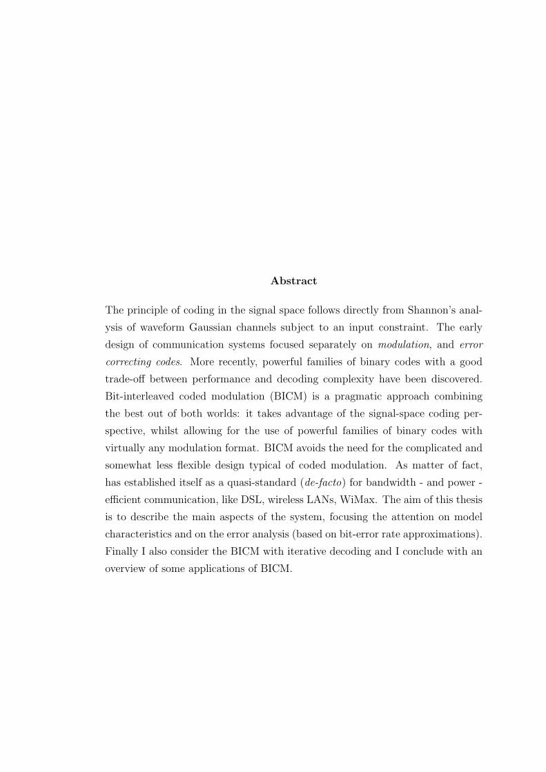
Abstract

The principle of coding in the signal space follows directly from Shannon’s anal-

ysis of waveform Gaussian channels subject to an input constraint. The early

design of communication systems focused separately on modulation, and error

correcting codes. More recently, powerful families of binary codes with a good

trade-off between performance and decoding complexity have been discovered.

Bit-interleaved coded modulation (BICM) is a pragmatic approach combining

the best out of both worlds: it takes advantage of the signal-space coding per-

spective, whilst allowing for the use of powerful families of binary codes with

virtually any modulation format. BICM avoids the need for the complicated and

somewhat less flexible design typical of coded modulation. As matter of fact,

has established itself as a quasi-standard (de-facto) for bandwidth - and power -

efficient communication, like DSL, wireless LANs, WiMax. The aim of this thesis

is to describe the main aspects of the system, focusing the attention on model

characteristics and on the error analysis (based on bit-error rate approximations).

Finally I also consider the BICM with iterative decoding and I conclude with an

overview of some applications of BICM.

Chapter 1

Introduction

Since Shannon’s landmark 1948 paper [1], approaching the capacity of the addi-

tive white Gaussian noise (AWGN) channel has been one of the more relevant

topics in information theory and coding theory. Shannon’s promise that rates up

to the channel capacity can be reliably transmitted over the channel comes to-

gether with the design challenge of effectively constructing coding schemes achiev-

ing these rates with limited encoding and decoding complexity. A simply way

of constructing codes for the Gaussian channel consists of fixing the modulator

signal set, and then considering codewords obtained as sequences over the fixed

modulator signal set, or alphabet.

Starting from the trellis-coded modulation analysed in [2], it has been generally

accepted that modulation and coding should be combined in a single entity for

improved performance, based on the combination of trellis codes and discrete

signal constellations through set partitioning. The code performance in this sit-

uation depends strongly, rather than on the minimum Euclidean distance of the

code, on its minimum Hamming distance (the ’code diversity’).

The discovery of turbo-codes and the re-discovery of low-density parity-check

(LDPC) codes, with their corresponding iterative decoding algorithms marked a

new era in coding theory. These modern codes approach the capacity of binary-

input channels with low-complexity. The analysis of iterative decoding also led

to new methods for their efficient design.

In contrast with findings in [2], in [3] is proposed the bit-interleaved coded modu-

lation (BICM) as a pragmatic approach to coded modulation. Here is recognized

that the code diversity, and hence the reliability of coded modulation over the

3

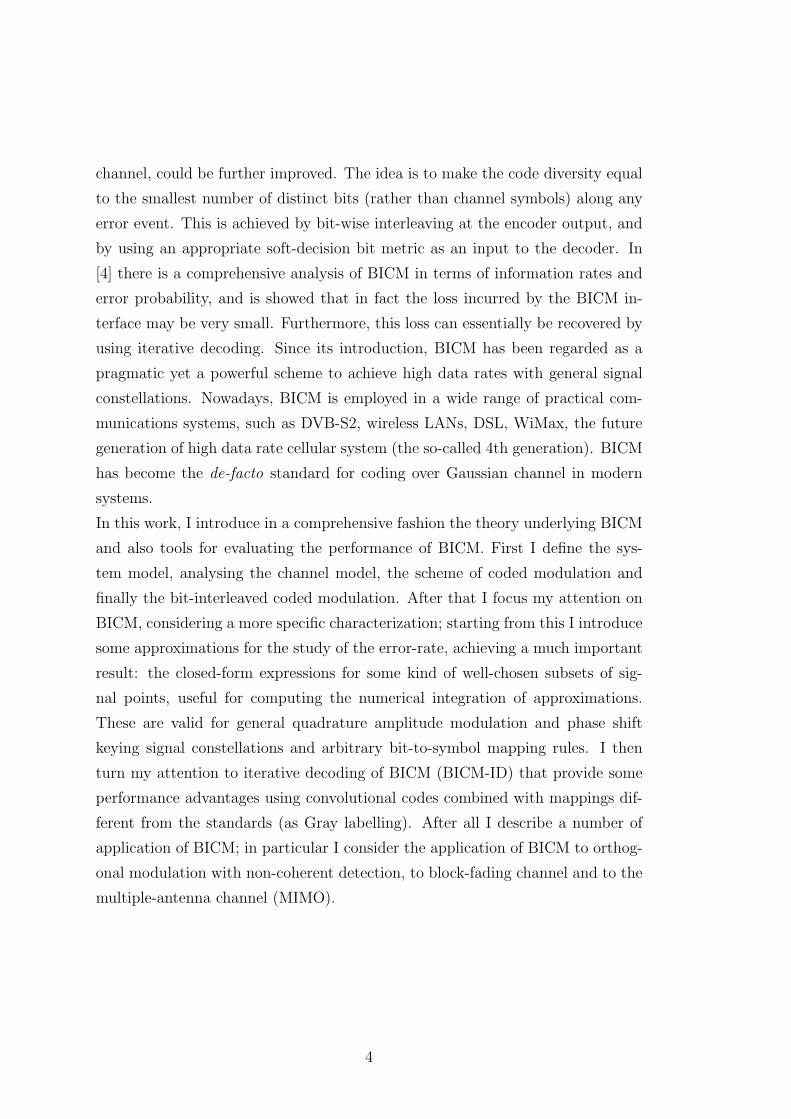
channel, could be further improved. The idea is to make the code diversity equal

to the smallest number of distinct bits (rather than channel symbols) along any

error event. This is achieved by bit-wise interleaving at the encoder output, and

by using an appropriate soft-decision bit metric as an input to the decoder. In

[4] there is a comprehensive analysis of BICM in terms of information rates and

error probability, and is showed that in fact the loss incurred by the BICM in-

terface may be very small. Furthermore, this loss can essentially be recovered by

using iterative decoding. Since its introduction, BICM has been regarded as a

pragmatic yet a powerful scheme to achieve high data rates with general signal

constellations. Nowadays, BICM is employed in a wide range of practical com-

munications systems, such as DVB-S2, wireless LANs, DSL, WiMax, the future

generation of high data rate cellular system (the so-called 4th generation). BICM

has become the de-facto standard for coding over Gaussian channel in modern

systems.

In this work, I introduce in a comprehensive fashion the theory underlying BICM

and also tools for evaluating the performance of BICM. First I define the sys-

tem model, analysing the channel model, the scheme of coded modulation and

finally the bit-interleaved coded modulation. After that I focus my attention on

BICM, considering a more specific characterization; starting from this I introduce

some approximations for the study of the error-rate, achieving a much important

result: the closed-form expressions for some kind of well-chosen subsets of sig-

nal points, useful for computing the numerical integration of approximations.

These are valid for general quadrature amplitude modulation and phase shift

keying signal constellations and arbitrary bit-to-symbol mapping rules. I then

turn my attention to iterative decoding of BICM (BICM-ID) that provide some

performance advantages using convolutional codes combined with mappings dif-

ferent from the standards (as Gray labelling). After all I describe a number of

application of BICM; in particular I consider the application of BICM to orthog-

onal modulation with non-coherent detection, to block-fading channel and to the

multiple-antenna channel (MIMO).

4

Chapter 2

System model

In this chapter I recall the baseline model of coded modulation(CM) and introduce

the model of bit-interleaved coded modulation(BICM). Here I consider a generic

stationary finite-memory vector channel, that in the next analysis will be more

specified.

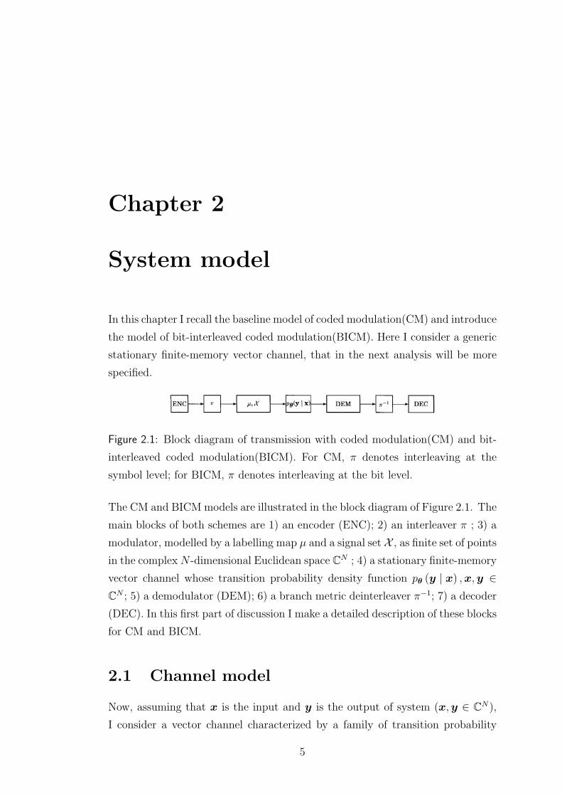
Figure 2.1: Block diagram of transmission with coded modulation(CM) and bit-

interleaved coded modulation(BICM). For CM, π denotes interleaving at the

symbol level; for BICM, π denotes interleaving at the bit level.

The CM and BICM models are illustrated in the block diagram of Figure 2.1. The

main blocks of both schemes are 1) an encoder (ENC); 2) an interleaver π ; 3) a

modulator, modelled by a labelling map µ and a signal set X , as finite set of points

in the complexN -dimensional Euclidean space CN ; 4) a stationary finite-memory

vector channel whose transition probability density function pθ (y | x) ,x,y ∈CN ; 5) a demodulator (DEM); 6) a branch metric deinterleaver π−1; 7) a decoder

(DEC). In this first part of discussion I make a detailed description of these blocks

for CM and BICM.

2.1 Channel model

Now, assuming that x is the input and y is the output of system (x,y ∈ CN),

I consider a vector channel characterized by a family of transition probability

5

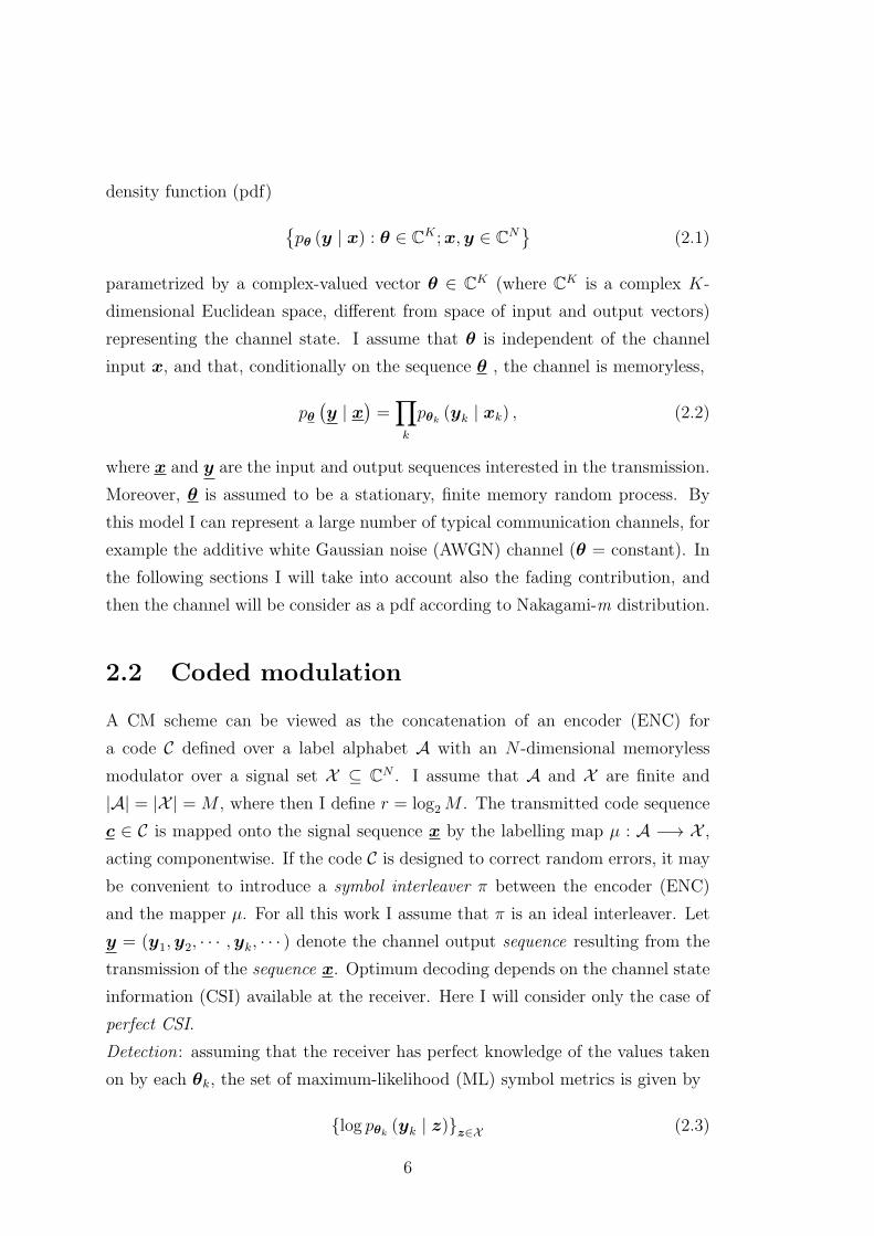
density function (pdf) {pθ (y | x) : θ ∈ CK ;x,y ∈ CN

}(2.1)

parametrized by a complex-valued vector θ ∈ CK (where CK is a complex K-

dimensional Euclidean space, different from space of input and output vectors)

representing the channel state. I assume that θ is independent of the channel

input x, and that, conditionally on the sequence θ , the channel is memoryless,

pθ(y | x

)=∏k

pθk(yk | xk) , (2.2)

where x and y are the input and output sequences interested in the transmission.

Moreover, θ is assumed to be a stationary, finite memory random process. By

this model I can represent a large number of typical communication channels, for

example the additive white Gaussian noise (AWGN) channel (θ = constant). In

the following sections I will take into account also the fading contribution, and

then the channel will be consider as a pdf according to Nakagami-m distribution.

2.2 Coded modulation

A CM scheme can be viewed as the concatenation of an encoder (ENC) for

a code C defined over a label alphabet A with an N -dimensional memoryless

modulator over a signal set X ⊆ CN . I assume that A and X are finite and

|A| = |X | = M , where then I define r = log2 M . The transmitted code sequence

c ∈ C is mapped onto the signal sequence x by the labelling map µ : A −→ X ,

acting componentwise. If the code C is designed to correct random errors, it may

be convenient to introduce a symbol interleaver π between the encoder (ENC)

and the mapper µ. For all this work I assume that π is an ideal interleaver. Let

y = (y1,y2, · · · ,yk, · · · ) denote the channel output sequence resulting from the

transmission of the sequence x. Optimum decoding depends on the channel state

information (CSI) available at the receiver. Here I will consider only the case of

perfect CSI.

Detection: assuming that the receiver has perfect knowledge of the values taken

on by each θk, the set of maximum-likelihood (ML) symbol metrics is given by

{log pθk(yk | z)}z∈X (2.3)

6

After metric deinterleaving (denoted by π−1 in Figure 2.1), ML decision about

the transmitted code sequence is made according to the rule,

c = argmaxc∈C

∑k

log pθk(yk | µ(ck)) (2.4)

where the summation runs over the whole sequence. This equation represents the

ML decision rule also with finite-depth or with no interleaving, since conditionally

on θ, the channel is memoryless.

2.3 Bit-interleaved coded modulation

BICM can be obtained by concatenating an encoder ENC for binary code C, withan N -dimensional memoryless modulator over a signal set X ⊆ CN of size |X | =M = 2r, through a bit interleaver π and a one-to-one binary labelling map µ :

{0, 1}r → X . The code sequence c is first interleaved by π. Next, the interleaved

sequence π (c) is broken into subsequences of r bits each, which are mapped onto

signals in X . Finally, the resulting signal sequence x is transmitted over the

vector channel. The bit interleaver can be seen as a one-to-one correspondence

π :→ (k′, i), where k denotes the time ordering of the coded bits ck, k′ denotes

the time ordering of the signals x′k transmitted over the vector channel, and i

indicates the position of the bit ck in the label of x′k. From here I assume ideal

bit interleaving to make simplified analysis. Let l i (x) denote the ith bit of the

label of x, and X ib the subset of all the signals x ∈ X whose label has the value

b ∈ {0, 1} in position i. Further, let b denote the complement of b and y the

channel output resulting from the transmission of x. The conditional pdf of y,

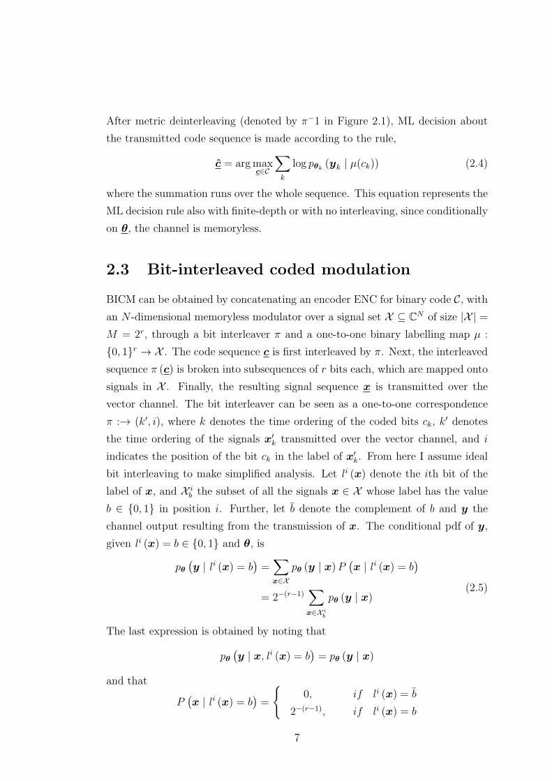
given l i (x) = b ∈ {0, 1} and θ, is

pθ(y | l i (x) = b

)=∑x∈X

pθ (y | x)P(x | l i (x) = b

)= 2−(r−1)

∑x∈X i

b

pθ (y | x)(2.5)

The last expression is obtained by noting that

pθ(y | x, l i (x) = b

)= pθ (y | x)

and that

P(x | l i (x) = b

)=

{0, if l i (x) = b

2−(r−1), if l i (x) = b

7

where I assume uniform input distribution

P (b = 0) = P (b = 1) =1

2

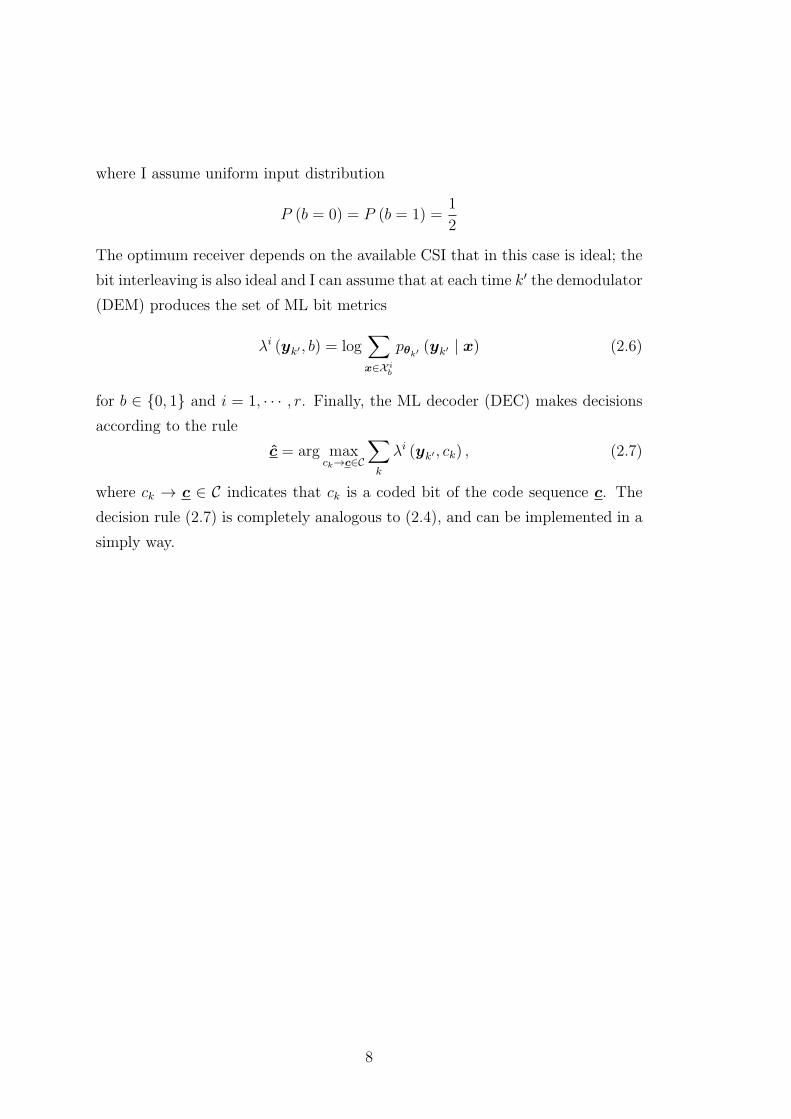
The optimum receiver depends on the available CSI that in this case is ideal; the

bit interleaving is also ideal and I can assume that at each time k′ the demodulator

(DEM) produces the set of ML bit metrics

λi (yk′ , b) = log∑x∈X i

b

pθk′(yk′ | x) (2.6)

for b ∈ {0, 1} and i = 1, · · · , r. Finally, the ML decoder (DEC) makes decisions

according to the rule

c = arg maxck→c∈C

∑k

λi (yk′ , ck) , (2.7)

where ck → c ∈ C indicates that ck is a coded bit of the code sequence c. The

decision rule (2.7) is completely analogous to (2.4), and can be implemented in a

simply way.

8

Chapter 3

BICM analysis and

approximations

After the introduction to the system model of previous chapter, I want to get

a more specific characterization for BICM systems. As in my analysis I will

consider the transmission performances over fading channels, I use a Nakagami-

m distribution to model the channel aspects. Assuming this, I evaluate some

approximations for the error-rate, comparing the results with union bound found

in [4]. This work is very useful for the system design and in next sections I will

derive other simplified expressions for this purpose.

Figure 3.1: Block diagram of BICM transmission over a fading AWGN channel.

3.1 Preliminaries

Figure 3.1 shows the block diagram of equivalent BICM transmission system:

Transmitter: The BICM codeword x = [x1, x2, · · · , xL] ∈ C comprises L complex

9

valued symbols and is obtained by first interleaving (π) the output of a binary

encoder c = [c1, c2, · · · , cN ] into cπ = [cπ1 , cπ2 , · · · , cπN ] and a subsequent mapping

µ : {0, 1}r → X of each r = log2 (M) bits. While the pdf approximation that

I will present next is applicable to arbitrary signal constellations, for practical

relevance I assume that X is an M -ary QAM or PSK constellation with average

unit symbol energy. As usual, the coding and mapping results in a uniform dis-

tribution signal points. When presenting numerical results next, I consider set

Figure 3.2: 16QAM signal set with (a) a suitable set partitioning labelling and

(b) Gray Labelling.

partitioning labelling (SPL), semi set partitioning labelling (SSPL), modified set

partitioning labelling (MSPL), and mixed labelling (ML), in addition to popular

Gray labelling (GL) for QAM and PSK signal constellations. As Gray labelling

plays a key role in BICM theory, I restate here its definition in term of BICM

notation: let X denote a signal set of size M = 2r, with minimum Euclidean

distance dmin. A binary map µ : {0, 1}r → X is a Gray labelling for X if, for

all i = 1, · · · , r and b ∈ {0, 1}, each x ∈ X ib has at most one z ∈ X i

bat distance

dmin. Figure 3.2 shows a labelled 16QAM signal set.

Channel: I consider BICM transmission over AWGN channels. The equivalent

baseband discrete-time transmission model can be written as

yi =√γhixi + zi, (3.1)

where yi ∈ C is the received sample, hi ∈ R denotes the fading gain, zi ∈ C is

the additive noise sample at discrete-time i. The noise samples are independent

10

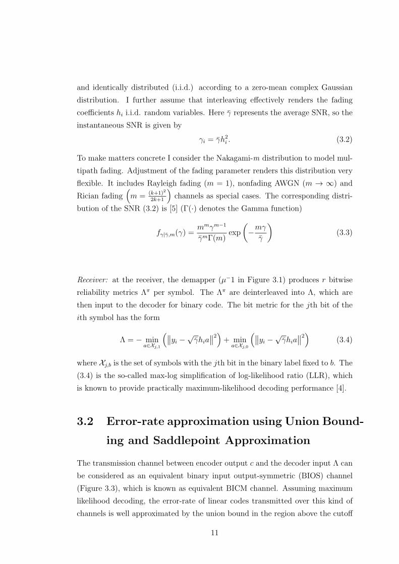
and identically distributed (i.i.d.) according to a zero-mean complex Gaussian

distribution. I further assume that interleaving effectively renders the fading

coefficients hi i.i.d. random variables. Here γ represents the average SNR, so the

instantaneous SNR is given by

γi = γh2i . (3.2)

To make matters concrete I consider the Nakagami-m distribution to model mul-

tipath fading. Adjustment of the fading parameter renders this distribution very

flexible. It includes Rayleigh fading (m = 1), nonfading AWGN (m → ∞) and

Rician fading(m = (k+1)2

2k+1

)channels as special cases. The corresponding distri-

bution of the SNR (3.2) is [5] (Γ(·) denotes the Gamma function)

fγ|γ,m(γ) =mmγm−1

γmΓ(m)exp

(−mγ

γ

)(3.3)

Receiver: at the receiver, the demapper (µ−1 in Figure 3.1) produces r bitwise

reliability metrics Λπ per symbol. The Λπ are deinterleaved into Λ, which are

then input to the decoder for binary code. The bit metric for the jth bit of the

ith symbol has the form

Λ = − mina∈Xj,1

(∥∥yi −√γhia

∥∥2)+ mina∈Xj,0

(∥∥yi −√γhia

∥∥2) (3.4)

where Xj,b is the set of symbols with the jth bit in the binary label fixed to b. The

(3.4) is the so-called max-log simplification of log-likelihood ratio (LLR), which

is known to provide practically maximum-likelihood decoding performance [4].

3.2 Error-rate approximation using Union Bound-

ing and Saddlepoint Approximation

The transmission channel between encoder output c and the decoder input Λ can

be considered as an equivalent binary input output-symmetric (BIOS) channel

(Figure 3.3), which is known as equivalent BICM channel. Assuming maximum

likelihood decoding, the error-rate of linear codes transmitted over this kind of

channels is well approximated by the union bound in the region above the cutoff

11

Figure 3.3: BIOS channel.

rate. As can be seen in [4], the BER union bound for a convolutional code of rate

Rc = kc/nc is given by

Pb ≤1

kc

∞∑dH=dH,min

wdHPEP (dH | γ,m) (3.5)

where wdH denotes total input weight of error events at Hamming distance dH ,

dH,min denotes the free distance of the convolutional code, and PEP (dH | γ,m)

is the pairwise error probability corresponding to an error event with Hamming

weight dH . For BIOS channels, the PEP can be considered as the tail probability

of a random variable generated by summing dH i.i.d LLRs Λ1, · · · ,ΛdH . Choosing

all-one codeword as reference codeword, I get

PEP (dH | γ,m) = P

(∆dH =

dH∑i=1

Λi < 0 | γ,m

). (3.6)

For computing such a probability, a common way is through the use of the Laplace

transform ΦΛ|γ,m (s) of the pdf of Λ. That is

P (∆dH < 0 | γ,m) =1

2πj

∫ α+∞

α−∞

[ΦΛ|γ,m (s)

]dH ds

s, (3.7)

where j is the imaginary unit and α ∈ R, 0 < α < αmax, is chosen in the region

of convergence of integral. The computation of this is often not straightforward

and invokes the use of numerical methods. For this reason in [6] are proposed a

few bounds and estimations; one of the most important for its simply form and

accuracy is the saddlepoint approximations, that get an approximation for the

previous result:

P (∆dH < 0 | γ,m) ≈(ΦΛ|γ,m (s)

)dH+0.5

s√2πdHΦ′′

Λ|γ,m (s), (3.8)

12

where Φ′′Λ|γ,m (s) denotes the second-order derivative of ΦΛ|γ,m (s) and s ∈ R+,

0 < s < αmax, is the saddlepoint defined through the first-order derivative as

Φ′Λ|γ,m (s) = 0. (3.9)

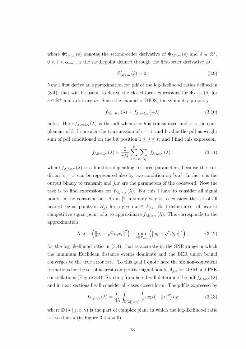
Now I first derive an approximation for pdf of the log-likelihood ratios defined in

(3.4), that will be useful to derive the closed-form expressions for ΦΛ|γ,m (s) for

s ∈ R+ and arbitrary m. Since the channel is BIOS, the symmetry property

fΛ|c=b,γ (λ) = fΛ|c=b,γ (−λ) (3.10)

holds. Here fΛ|c=b,γ (λ) is the pdf when c = b is transmitted and b is the com-

plement of b. I consider the transmission of c = 1, and I value the pdf as weight

sum of pdf conditioned on the bit position 1 ≤ j ≤ r, and I find this expression

fΛ|c=1,γ (λ) =2

rM

r∑j=1

∑x∈Xj,1

fΛ|j,x,γ (λ) . (3.11)

where fΛ|j,x,γ (λ) is a function depending to three parameters, because the con-

dition ’c = 1’ can be represented also by two condition on ’j, x’. In fact c is the

output binary to transmit and j, x are the parameters of the codeword. Now the

task is to find expressions for fΛ|j,x,γ (λ). For this I have to consider all signal

points in the constellation. As in [7] a simply way is to consider the set of all

nearest signal points in Xj,b for a given x ∈ Xj,b. So I define a set of nearest

competitive signal point of x to approximate fΛ|j,x,γ (λ). This corresponds to the

approximation

Λ ≈ −(∥∥yi −√

γhixi

∥∥2)+ mina∈Xj,xi

(∥∥yi −√γhia

∥∥2) , (3.12)

for the log-likelihood ratio in (3.4), that is accurate in the SNR range in which

the minimum Euclidean distance events dominate and the BER union bound

converges to the true error rate. To this goal I quote here the six non-equivalent

formations for the set of nearest competitive signal points Aj,x for QAM and PSK

constellations (Figure 3.4). Starting from here I will determine the pdf fΛ|j,x,γ (λ)

and in next sections I will consider all-cases closed-form. The pdf is expressed by

fΛ|j,x,γ (λ) =d

dλ

∫D(λ|j,x,γ)

1

πexp

(−∥z∥2

)dz (3.13)

where D (λ | j, x, γ) is the part of complex plane in which the log-likelihood ratio

is less than λ (in Figure 3.4 λ = 0)

13

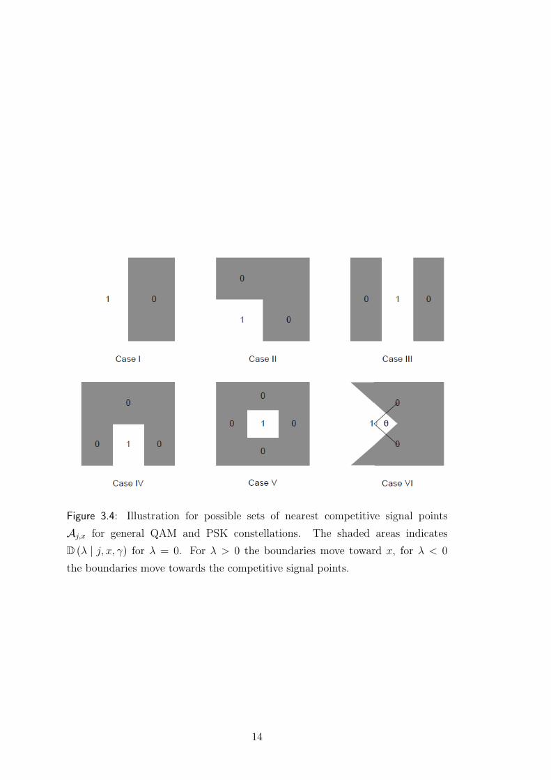
Figure 3.4: Illustration for possible sets of nearest competitive signal points

Aj,x for general QAM and PSK constellations. The shaded areas indicates

D (λ | j, x, γ) for λ = 0. For λ > 0 the boundaries move toward x, for λ < 0

the boundaries move towards the competitive signal points.

14

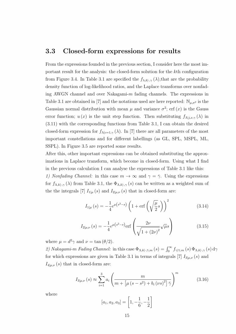
3.3 Closed-form expressions for results

From the expressions founded in the previous section, I consider here the most im-

portant result for the analysis: the closed-form solution for the kth configuration

from Figure 3.4. In Table 3.1 are specified the fλ,k|·,γ (λ),that are the probability

density function of log-likelihood ratios, and the Laplace transforms over nonfad-

ing AWGN channel and over Nakagami-m fading channels. The expressions in

Table 3.1 are obtained in [7] and the notations used are here reported: Nµ,σ2 is the

Gaussian normal distribution with mean µ and variance σ2; erf (x) is the Gauss

error function; u (x) is the unit step function. Then substituting fΛ|j,x,γ (λ) in

(3.11) with the corresponding functions from Table 3.1, I can obtain the desired

closed-form expression for fΛ|c=1,γ (λ). In [7] there are all parameters of the most

important constellations and for different labellings (as GL, SPL, MSPL, ML,

SSPL). In Figure 3.5 are reported some results.

After this, other important expressions can be obtained substituting the approx-

imations in Laplace transform, which become in closed-form. Using what I find

in the previous calculation I can analyse the expressions of Table 3.1 like this:

1) Nonfading Channel: in this case m → ∞ and γ = γ. Using the expressions

for fΛ,k|·,γ (λ) from Table 3.1, the ΦΛ,k|·,γ (s) can be written as a weighted sum of

the the integrals [7] I1|µ (s) and I2|µ,ν (s) that in closed-form are:

I1|µ (s) = −1

4eµ(s

2−s)(1 + erf

(õ

2s

))2

(3.14)

I2|µ,ν (s) = −1

4eµ(s

2−s)erf

2ν√1 + (2ν)2

õs

(3.15)

where µ = d2γ and ν = tan (θ/2).

2) Nakagami-m Fading Channel: in this case ΦΛ,k|·,γ,m (s) =∫∞0

fγ|γ,m (s) ΦΛ,k|·,γ (s) dγ

for which expressions are given in Table 3.1 in terms of integrals [7] I3|µ,ν (s) and

I4|µ,ν (s) that in closed-form are:

I3|µ,ν (s) ≈3∑

i=1

ai

(m

m+[µ (s− s2) + bi (νs)

2] γ)m

(3.16)

where

[a1, a2, a3] =

[1,−1

6,−1

2

]15

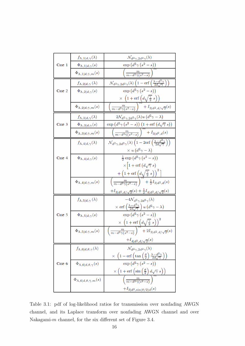
Table 3.1: pdf of log-likelihood ratios for transmission over nonfading AWGN

channel, and its Laplace transform over nonfading AWGN channel and over

Nakagami-m channel, for the six different set of Figure 3.4.

16

Figure 3.5: pdf of reliability metrics for BICM transmission over the nonfading

AWGN channel for different constellations and labelling. Lines are pdf approxi-

mations founded while markers represent the estimated histograms through sim-

ulative measurement.

17

and

[b1, b2, b3] =

[0, 1,

4

3

].

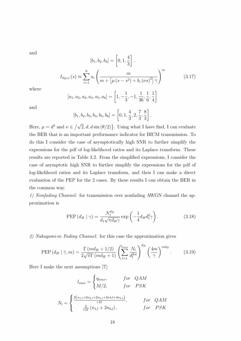
I4|µ,ν (s) ≈6∑

i=1

ai

(m

m+[µ (s− s2) + bi (νs)

2] γ)m

(3.17)

where

[a1, a2, a3, a4, a5, a6] =

[1,−1

3,−1,

1

36,1

6,1

4

]and

[b1, b2, b3, b4, b5, b6] =

[0, 1,

4

3, 2,

7

3,8

3

].

Here, µ = d2 and ν ∈/√

2, d, d sin (θ/2)}. Using what I have find, I can evaluate

the BER that is an important performance indicator for BICM transmission. To

do this I consider the case of asymptotically high SNR to further simplify the

expressions for the pdf of log-likelihood ratios and its Laplace transform. These

results are reported in Table 3.2. From the simplified expressions, I consider the

case of asymptotic high SNR to further simplify the expressions for the pdf of

log-likelihood ratios and its Laplace transform, and then I can make a direct

evaluation of the PEP for the 2 cases. By these results I can obtain the BER in

the common way.

1) Nonfading Channel: for transmission over nonfading AWGN channel the ap-

proximation is

PEP (dH | γ) = NdH1

d1√πdHγ

exp

(−1

4dHd

21γ

). (3.18)

2) Nakagami-m Fading Channel: for this case the approximation gives

PEP (dH | γ,m) =Γ (mdH + 1/2)

2√πΓ (mdH + 1)

(lmax∑l=1

Nl

d2ml

)dH (4m

γ

)mdH

. (3.19)

Here I make the next assumptions [7]:

lmax =

{qmax, for QAM

M/2, for PSK

Nl =

2(n1,l+2n2,l+2n3,l+3n4,l+4n5,l)

rM, for QAM

2rM

(n1,l + 2n6,l) , for PSK

18

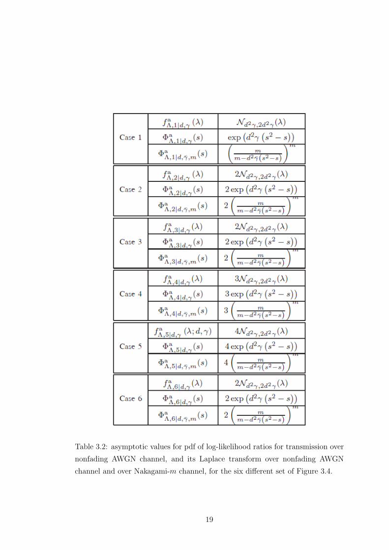
Table 3.2: asymptotic values for pdf of log-likelihood ratios for transmission over

nonfading AWGN channel, and its Laplace transform over nonfading AWGN

channel and over Nakagami-m channel, for the six different set of Figure 3.4.

19

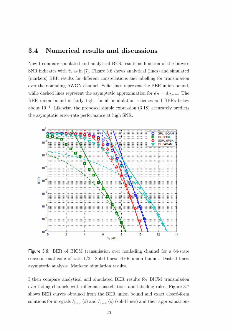
3.4 Numerical results and discussions

Now I compare simulated and analytical BER results as function of the bitwise

SNR indicates with γb as in [7]. Figure 3.6 shows analytical (lines) and simulated

(markers) BER results for different constellations and labelling for transmission

over the nonfading AWGN channel. Solid lines represent the BER union bound,

while dashed lines represent the asymptotic approximation for dH = dH,min. The

BER union bound is fairly tight for all modulation schemes and BERs below

about 10−4. Likewise, the proposed simple expression (3.18) accurately predicts

the asymptotic error-rate performance at high SNR.

Figure 3.6: BER of BICM transmission over nonfading channel for a 64-state

convolutional code of rate 1/2. Solid lines: BER union bound. Dashed lines:

asymptotic analysis. Markers: simulation results.

I then compare analytical and simulated BER results for BICM transmission

over fading channels with different constellations and labelling rules. Figure 3.7

shows BER curves obtained from the BER union bound and exact closed-form

solutions for integrals I3|µ,ν (s) and I4|µ,ν (s) (solid lines) and their approximations

20

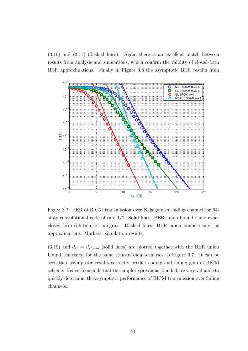
(3.16) and (3.17) (dashed lines). Again there is an excellent match between

results from analysis and simulations, which confirm the validity of closed-form

BER approximations. Finally in Figure 3.8 the asymptotic BER results from

Figure 3.7: BER of BICM transmission over Nakagami-m fading channel for 64-

state convolutional code of rate 1/2. Solid lines: BER union bound using exact

closed-form solution for integrals. Dashed lines: BER union bound using the

approximations. Markers: simulation results.

(3.19) and dH = dH,min (solid lines) are plotted together with the BER union

bound (markers) for the same transmission scenarios as Figure 3.7. It can be

seen that asymptotic results correctly predict coding and fading gain of BICM

scheme. Hence I conclude that the simple expressions founded are very valuable to

quickly determine the asymptotic performance of BICM transmission over fading

channels.

21

Figure 3.8: BER of BICM transmission over Nakagami-m fading channel for 64-

state convolutional code of rate 1/2. Solid lines: asymptotic analysis with (3.19).

Markers: BER union bound.

22

Chapter 4

Introduction of iterative decoding

In this chapter, I study BICM with iterative decoding (BICM-ID). Inspired by

the advent of turbo-codes and iterative decoding, BICM-ID was proposed in

order to improve the performance of BICM by exchanging messages between

the demodulator and the decoder of the underlying binary code. As illustrated

in Figure 4.1 and shown in [8], [9], BICM-ID can provide some performance

advantages using convolutional codes combined with mapping different from Gray.

With this kind of system with 8-state convolutional code of rate-2/3, and 8-

PSK modulation, using hard-decision feedback, achieves an improvement over the

conventional BICM scheme that exceeds 1 dB for a fully-interleaved Rayleigh flat-

fading channel and that exceeds 1.5 dB for a channel with additive white Gaussian

noise. This robust performance makes BICM with iterative decoding suitable for

both types of channels [8]. In this analysis I will use only a system with this

characteristics (8-state convolutional code of rate-2/3, and 8-PSK modulation);

the extension to other coding rates and modulation types is straightforward.

4.1 System description

The system block is shown in Figure 4.2. Note the addition of a feedback loop

compared with the conventional decoder. I represent the output of the encoder

by

C =[c10, c

20, c

30, · · · , c1t , c2t , c3t , · · ·

]= [C0, · · · , Ct, · · · ] (4.1)

where cit is the ith output bit at time position t and Ct = [c1t , c2t , c

3t ]. Three inde-

pendent bit interleavers permute bits to break the correlation of fading channels

23

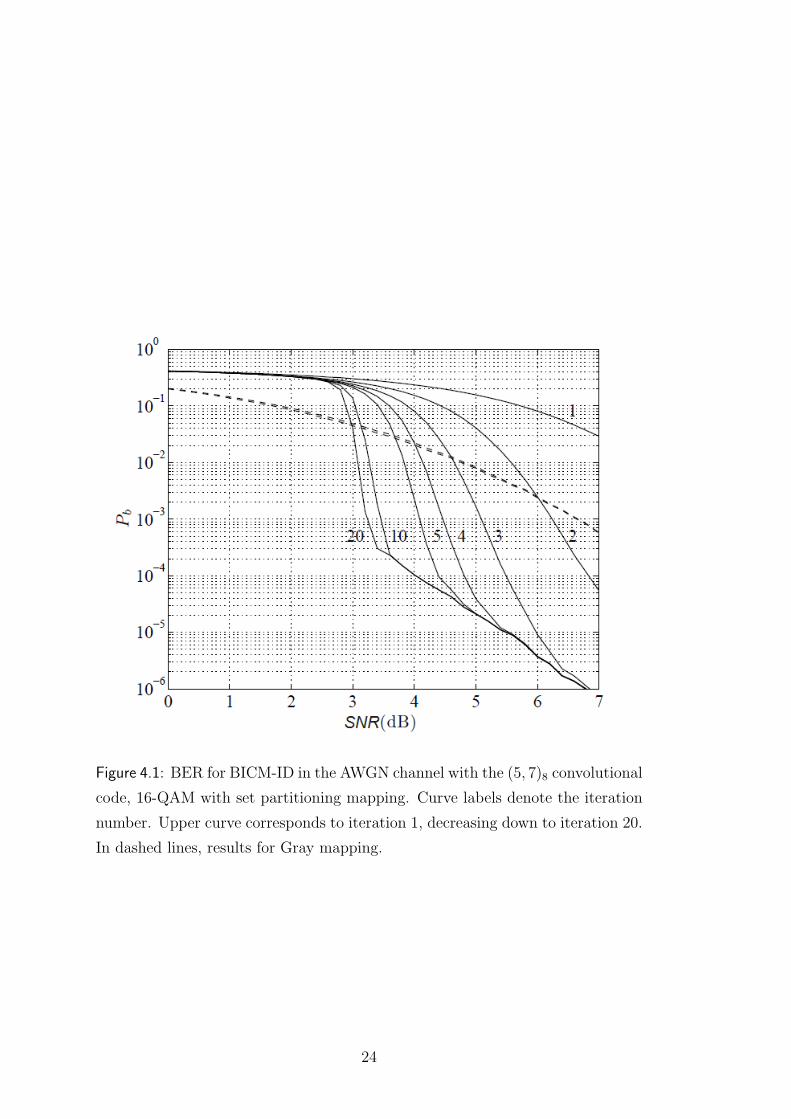
Figure 4.1: BER for BICM-ID in the AWGN channel with the (5, 7)8 convolutional

code, 16-QAM with set partitioning mapping. Curve labels denote the iteration

number. Upper curve corresponds to iteration 1, decreasing down to iteration 20.

In dashed lines, results for Gray mapping.

24

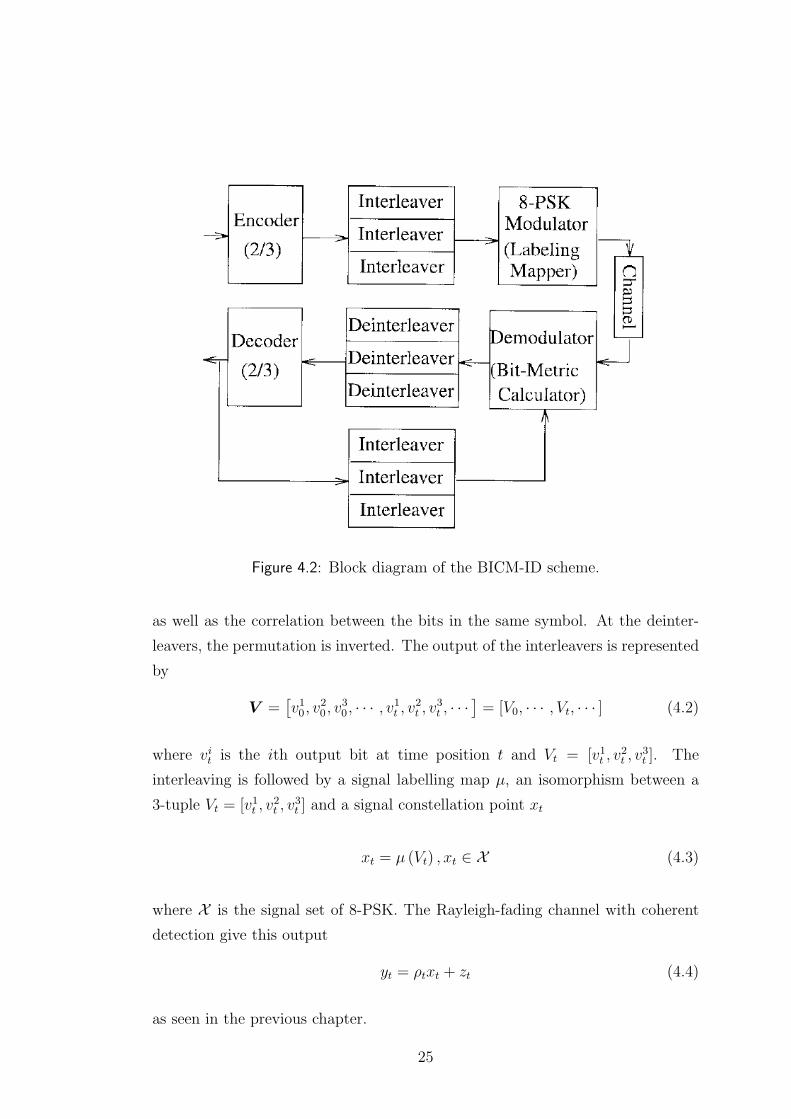
Figure 4.2: Block diagram of the BICM-ID scheme.

as well as the correlation between the bits in the same symbol. At the deinter-

leavers, the permutation is inverted. The output of the interleavers is represented

by

V =[v10, v

20, v

30, · · · , v1t , v2t , v3t , · · ·

]= [V0, · · · , Vt, · · · ] (4.2)

where vit is the ith output bit at time position t and Vt = [v1t , v2t , v

3t ]. The

interleaving is followed by a signal labelling map µ, an isomorphism between a

3-tuple Vt = [v1t , v2t , v

3t ] and a signal constellation point xt

xt = µ (Vt) , xt ∈ X (4.3)

where X is the signal set of 8-PSK. The Rayleigh-fading channel with coherent

detection give this output

yt = ρtxt + zt (4.4)

as seen in the previous chapter.

25

4.2 Conventional decoding

For each received signal yt, a log-likelihood function is calculated for the two

possible binary values of each coded bit

λ(vit = b

)= log

∑x∈X (i,b)

P (x | yt, ρt)

= log

∑x∈X (i,b)

P (yt | x, ρt)P (x)

,

i = 1, 2, 3; b = 0, 1

(4.5)

where the signal subset X (i, b) = {µ (v1, v2, v3) | vi = b} and the terms common

to all i and b are disregarded. In conventional decoding, the a priori probability

P (x) is assumed equal for any x ∈ X (i, b). Then, the bit metric becomes

λ(vit = b

)= log

∑x∈X (i,b)

P (yt | x, ρt)

≈ maxx∈X (i,b)

logP (yt | x, ρt)

= − minx∈X (i,b)

∥yt − ρtx∥2

(4.6)

where a constant scalar is disregarded and the approximation is good at high

SNR. At the decoder (as Viterbi decoder), the branch metric corresponding to

each of the eight possible 3-tuple is the sum of the corresponding bit metrics after

deinterleaving.

4.3 Iterative decoding with hard-decision feed-

back

Convolutional encoding introduces redundancy and memory into the signal se-

quence. Yet, the equally likely assumption made before fails to use this informa-

tion, primarily because it is difficult to specify in advance of any decoding. The

a priori information is reflected in the decoding results and therefore can be in-

cluded through iterative decoding. One approach is to use the Viterbi algorithm

(see Appendix A) with soft outputs, although this is computationally complex.

Instead, I consider only binary-decision feedback for the calculation of the bit

26

metrics in the second round of decoding. For example, to calculate λ (v1t = 0) I

assume, for any x = µ (v1 = 0, v2, v3) ∈ X (1, 0),

P (x) =

{1, if v1 = 0, v2 = v2t , v

3 = v3t

0, otherwise(4.7)

where v2t and v3t are the first-round decoding decisions. Then the bit metric with

the decision feedback becomes

λ(v1t = 0

)= −

∥∥yt − ρtµ(0, v2t , v

3t

)∥∥2 . (4.8)

The bit metrics for other bit positions and bit values follow similarly. Given the

feedback v2t and v3t the Euclidean distance between the signals µ (0, v2t , v3t ) and

µ (1, v2t , v3t ) can be significantly larger than the minimum Euclidean distance be-

tween the signals in the subset X (1, 0) and those X (1, 1). With an appropriate

signal labelling, the minimum Euclidean distance between coded sequences can

be made large for BICM-ID. This is the key that BICM-ID outperforms con-

ventional BICM. To avoid severe error propagation, the bits feedback should be

independent of the bit for which the bit metric is calculated. This is made possible

by independent bit interleavers - the three bits making up a channel symbol are

typically far apart in the coded sequence. This is clearly a feature not available

in a symbol-interleaved system.

4.4 Signal labelling

The performance of BICM-ID strongly depends on the signal labelling methods.

It can be seen that a mixed labelling method outperforms both Gray labelling

and set-partitioning labelling. With mixed labelling, the eight sequential labels

for 8-PSK signals are {000, 001, 010, 011, 110, 111, 100, 101}. The details of the

labelling design are discussed in [9]. Here I report only the results.

4.5 Simulation results

Now I show the BER performance of 8-PSK BICM-ID for both Rayleigh fading

and AWGN channels. Also other type of scheme are included for comparison.

The performance for Rayleigh fading channels is shown in Figure 4.3.

27

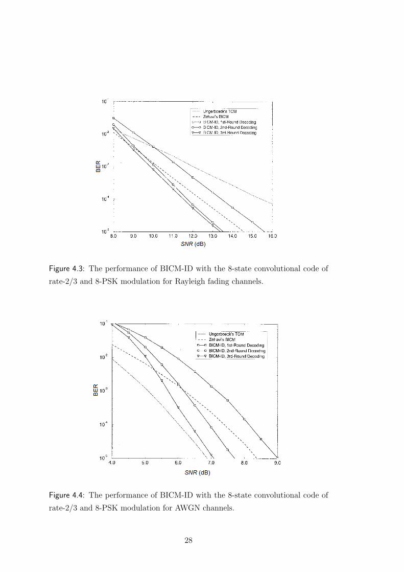
Figure 4.3: The performance of BICM-ID with the 8-state convolutional code of

rate-2/3 and 8-PSK modulation for Rayleigh fading channels.

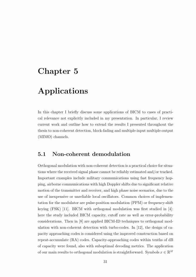
Figure 4.4: The performance of BICM-ID with the 8-state convolutional code of

rate-2/3 and 8-PSK modulation for AWGN channels.

28

Compared with BICM scheme proposed in Chapter 2, there is a 1 dB perfor-

mance degradation after the first round of decoding (without decision feedback)

of BICM-ID due to mixed labelling. However, with a second round of decoding,

BICM-ID quickly catches up and outperforms BICM by 1 dB. A third round of

decoding adds a slight improvement. The performance for AWGN channels is

shown in Figure 4.4. The SNR gap between BICM-ID and TCM scheme is only

0.2 dB. The gain of BICM-ID over BICM is more than 1.5 dB.

29

30

Chapter 5

Applications

In this chapter I briefly discuss some applications of BICM to cases of practi-

cal relevance not explicitly included in my presentation. In particular, I review

current work and outline how to extend the results I presented throughout the

thesis to non-coherent detection, block-fading and multiple-input multiple-output

(MIMO) channels.

5.1 Non-coherent demodulation

Orthogonal modulation with non-coherent detection is a practical choice for situa-

tions where the received signal phase cannot be reliably estimated and/or tracked.

Important examples include military communications using fast frequency hop-

ping, airborne communications with high Doppler shifts due to significant relative

motion of the transmitter and receiver, and high phase noise scenarios, due to the

use of inexpensive or unreliable local oscillators. Common choices of implemen-

tation for the modulator are pulse-position modulation (PPM) or frequency-shift

keying (FSK) [11]. BICM with orthogonal modulation was first studied in [4]:

here the study included BICM capacity, cutoff rate as well as error-probability

considerations. Then in [8] are applied BICM-ID techniques to orthogonal mod-

ulation with non-coherent detection with turbo-codes. In [12], the design of ca-

pacity approaching codes is considered using the improved construction based on

repeat-accumulate (RA) codes. Capacity-approaching codes within tenths of dB

of capacity were found, also with suboptimal decoding metrics. The application

of our main results to orthogonal modulation is straightforward. Symbols x ∈ RM

31

belong now to an orthogonal modulation constellation, x ∈ X = {e1, · · · , eM},where ek = (0, · · · , 0︸ ︷︷ ︸

k−1

, 1, 0, · · · , 0︸ ︷︷ ︸M−k−1

) is a vector has all zeros except in the k-th posi-

tion, where there is a one. The received signal over a fading channel can still be

expressed by (3.1), where now y, z ∈ CM , they are vectors of dimension M . The

channel transition probability becomes

Pθ (y | x, h) = 1

πMe−∥y−

√γxh∥2 . (5.1)

Depending on the knowledge of the channel coefficients at the receiver, the decod-

ing metric might vary. In particular, for coherent detection the symbol decoding

metric for hypothesis x = ek satisfies q (x = ek, y) ∝ Pθ (y | x, h). Here q (x, y)

is a function that represents∑

k λi (yk′ , ck) of (2.7). When no knowledge of the

carrier phase is available at the receiver, then the symbol decoding metric for

hypothesis x = ek with coded modulation becomes [11]

q (x = ek, y) ∝ I0(2√γ|h|yk

)(5.2)

where I0(·) is the zero-th order Bessel function of the first kind and with some

abuse of notation let yk denote the k-th entry of the received signal vector y. The

bit metrics are

qj (bj (x) = b,y) =∑k′∈X j

b

I0(2√γ|h|y′k

)(5.3)

where now the set X jb is the set of indices from {0, · · · ,M − 1} with bit b in the j-

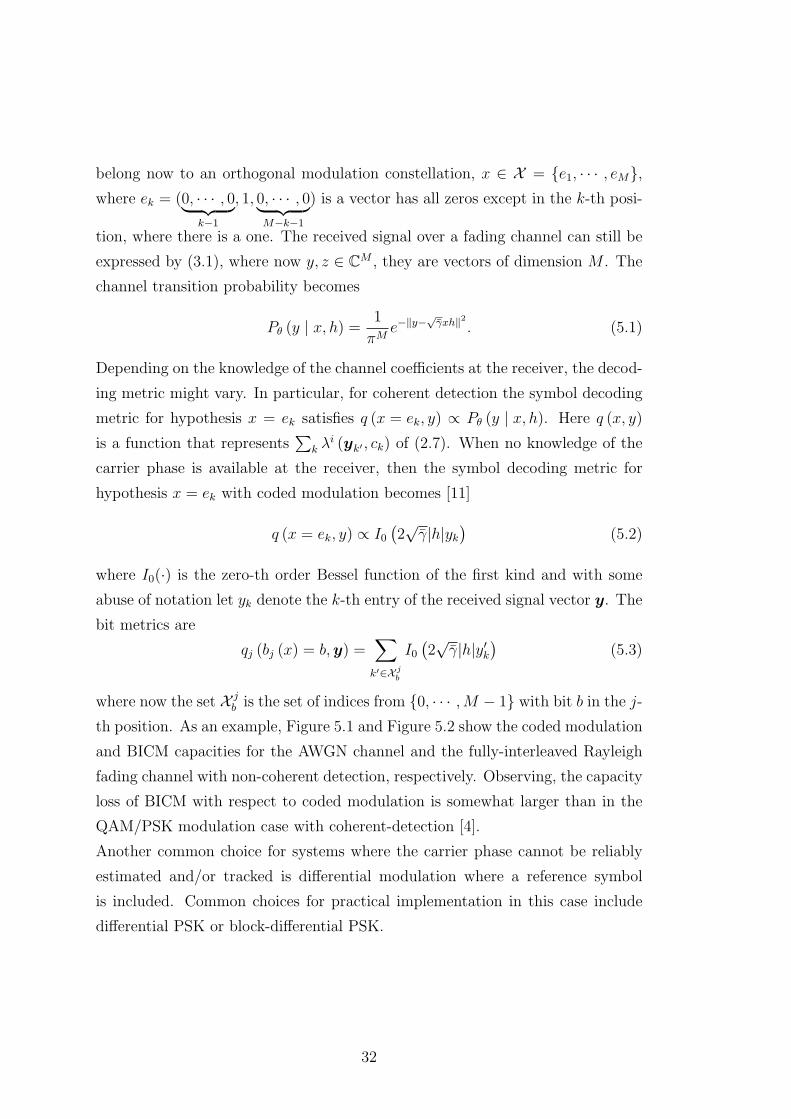
th position. As an example, Figure 5.1 and Figure 5.2 show the coded modulation

and BICM capacities for the AWGN channel and the fully-interleaved Rayleigh

fading channel with non-coherent detection, respectively. Observing, the capacity

loss of BICM with respect to coded modulation is somewhat larger than in the

QAM/PSK modulation case with coherent-detection [4].

Another common choice for systems where the carrier phase cannot be reliably

estimated and/or tracked is differential modulation where a reference symbol

is included. Common choices for practical implementation in this case include

differential PSK or block-differential PSK.

32

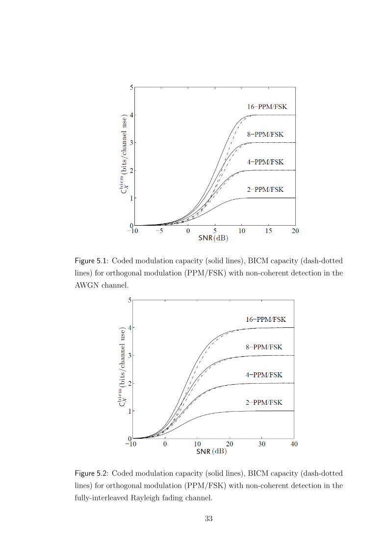
Figure 5.1: Coded modulation capacity (solid lines), BICM capacity (dash-dotted

lines) for orthogonal modulation (PPM/FSK) with non-coherent detection in the

AWGN channel.

Figure 5.2: Coded modulation capacity (solid lines), BICM capacity (dash-dotted

lines) for orthogonal modulation (PPM/FSK) with non-coherent detection in the

fully-interleaved Rayleigh fading channel.

33

5.2 Block-fading

The block-fading channel [13] is a useful channel model for a class of time - and/or

frequency - varying fading channels where the duration of a block-fading period

is determined by the product of the channel coherence bandwidth and the chan-

nel coherence time [11]. Within a block-fading period, the channel fading gain

remains constant. In this setting, transmission typically extends over multiple

block-fading periods. Frequency-hopping schemes as encountered in the Global

System for Mobile Communication (GSM) and the Enhanced Data GSM En-

vironment (EGDE), as well as transmission schemes based on OFDM, can also

conveniently be modelled as block-fading channels. The simplified model is math-

ematically tractable, while still capturing the essential features of the practical

transmission schemes over fading channels.

Denoting the number of block per codeword by B, the codeword transition prob-

ability in a block-fading channel can be expressed as

Pθ (y | x,h) =B∏i=1

N∏k=1

Pθi (yi,k | xi,k, hi) (5.4)

where xi,k, hi ∈ C are respectively the transmitted and received symbols at block

i and time k, and hi ∈ C is the channel coefficient corresponding to block i. The

symbol transition probability is given by

Pθi (yi,k | xi,k, hi) ∝ e−|yi,k−√γhixi,k|. (5.5)

The block-fading channel is equivalent to a set of parallel channels, each used a

fraction 1B

of the time. The block-fading channel is not information stable and

its channel capacity is zero. The corresponding information-theoretic limit is the

outage probability, and the design of efficient coded modulation schemes for the

block-fading channel is based on approaching the outage probability. In [14] it

was proved that the outage probability for sufficiently large SNR behaves as

Pout (SNR) = SNR−dsbK (5.6)

where dsb is the slope of the outage probability in a log-log scale and is given by

this bound

dsb = 1 +

⌊B

(1− R

r

)⌋. (5.7)

34

where the definition of r and R is the same that in Chapter 1. Hence, the error

probability of efficient coded modulation schemes in the block-fading channel

must have slope equal to this bound. Furthermore, this diversity is achievable by

coded modulation as well as BICM. As in Figure 5.3, the loss in outage probability

due to BICM is marginal. While the outage probability curves with Gaussian,

coded modulation and BICM inputs have the same slope dsb = 2 when B =

2, I note a change in the slope with coded modulation and BICM for B = 4.

This is due to the fact that while Gaussian inputs yield slope 4, the previous

bound gives dsb = 3. In [14] the family of blockwise concatenated codes based

on BICM was introduced. Improved binary codes for the block-fading channel

can be combined with blockwise bit interleaving to yield powerful BICM schemes.

Then, the error probability is averaged over the channel realizations. Similarly, in

order to characterize the error probability for the particular code constructions, I

need to calculate the error probability (or a bound) for each channel realization,

and average over the realizations. Unfortunately, the union bound averaged over

the channel realizations diverges, and improved bounds must be used. A simple,

yet very powerful technique, was proposed in [15], where the average over the

fading is performed once the union bound has been truncated at 1.

35

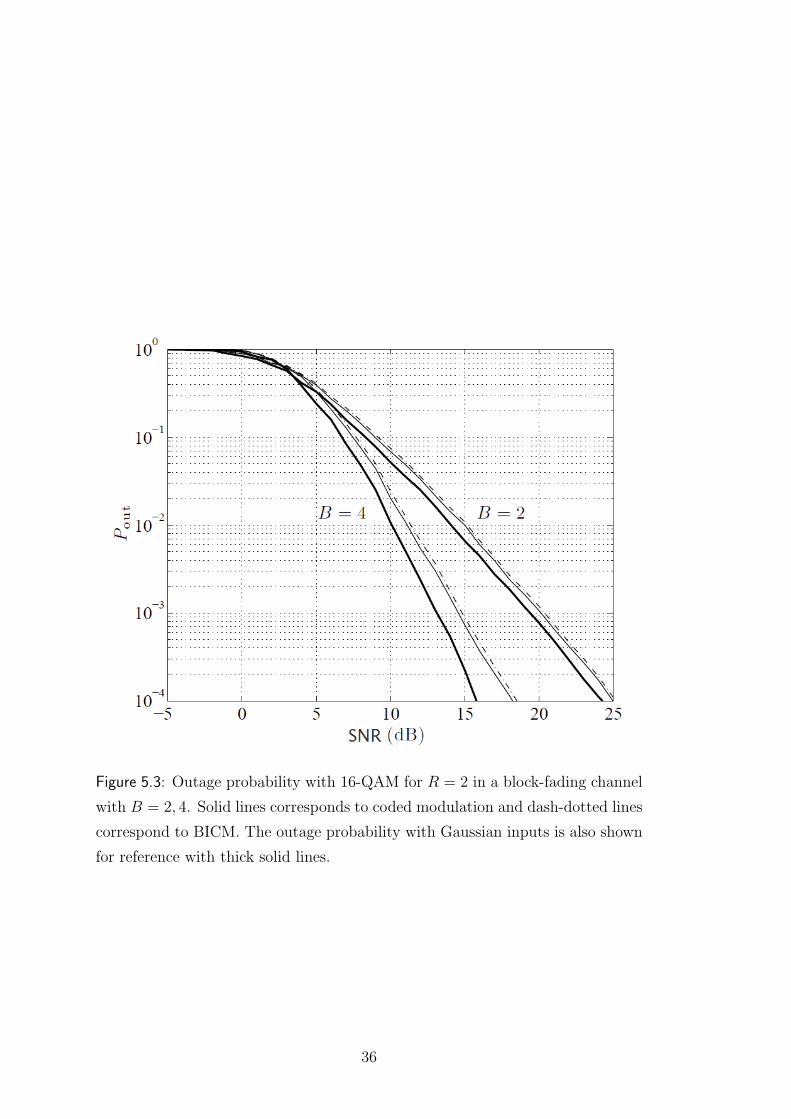
Figure 5.3: Outage probability with 16-QAM for R = 2 in a block-fading channel

with B = 2, 4. Solid lines corresponds to coded modulation and dash-dotted lines

correspond to BICM. The outage probability with Gaussian inputs is also shown

for reference with thick solid lines.

36

5.3 MIMO - Multiple Input Multiple Output

Channel fading often limits the reliability of wireless communications but diver-

sity can dramatically counteract the fading effects. Using several antennas at the

transmitter and at the receiver brings space diversity. Multiple-input multiple-

output (MIMO) systems can therefore offer an increased capacity and/or a better

transmission reliability. The target of most MIMO schemes is either to increase

the reliability by using the full diversity or to increase the bit rate by spatial mul-

tiplexing. Here I focus on a hybrid scheme. It is not a true spatial-multiplexing

scheme because redundant information is added in the sent signal by means of

bit-interleaved coded modulation [4]. This hybrid scheme can partially exploit

the transmit diversity but it cannot claim that it benefits from the full diversity.

It offers high flexibility because the encoder, the modulation and the number of

transmit antennas can be chosen independently.

Another recent powerful technique is iterative processing at the receiver. By

analogy with a turbo decoder, the iterations enable to jointly mitigate the inter-

ference and decode the bits (see Chapter 4). The turbo principle is well suited

to the MIMO BICM scheme because there is an encoder at the transmitter and

there is interference to deal with. Indeed, there is at least one kind of interference

with a MIMO BICM structure: it is the co-antenna interference (CAI), which is

due to the different signals that are simultaneously sent from the transmit an-

tennas. In the sequel, two low-complexity turbo receivers will be described. One

of them is well suited to a single-carrier (SC) modulation and the other one is

designed for an orthogonal frequency-division multiplexing (OFDM) modulation.

Then I show the ability of scheme to deal with the interference mitigation and

with the decoding, and to exploit the space diversity and the frequency diversity.

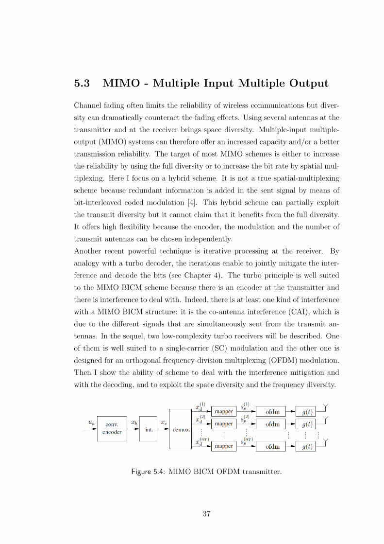
Figure 5.4: MIMO BICM OFDM transmitter.

37

Figure 5.5: MIMO BICM SC receiver.

Transmitter: The MIMO BICM transmitter is depicted in Figure 5.4. The infor-

mation bits are organized in frames. A frame of information bits is first encoded

by a rate-r convolutional encoder. The coded bits are then interleaved by a

random permutation. The frame of interleaved coded bits is then split into nT

sub-blocks, corresponding to the nT transmit antennas. Within each of these

sub-blocks, the interleaved coded bits are grouped and mapped to one of the

complex symbols in the considered multilevel/phase constellation. Figure 5.4

illustrates the OFDM transmitter. After the mapping, the symbols enter the

OFDM modulator and then the pulse-shaping filter. As far as the single-carrier

(SC) transmitter is concerned, the OFDM boxes have to be removed from the

figure and the pulse-shaping filter g (t) is applied before the SC modulation. Dur-

ing one symbol period T , nT symbols are transmitted: one per antenna. Since I

assume that the transmitter does not have any knowledge of the channel impulse

response, the antennas send signals with identical powers. They also use the same

shaping filter and the same modulation and mapping rule.

This transmitter enables to benefit from the transmit diversity because the coding

is performed before the frame is split between the antennas. Moreover, the pres-

ence of the bit-interleaver greatly reduces the correlation between successive coded

bits. The combination of the interleaver and the encoder enables to use the turbo

principle at the receiver. In the SC case, I can consider a bit-interleaved space-

time code because the redundant information added by the encoder is spread

over the space and time dimensions. In the OFDM case, I can consider a bit-

interleaved space-frequency code because this redundant information is spread

over the space and frequency dimensions. Note that both of these schemes offer

high flexibility because the encoder, the modulation and the number of transmit

antennas can be chosen independently.

38

Figure 5.6: MIMO BICM OFDM receiver.

Receiver: Both receivers follow the same outline. They are iterative and make use

of the turbo principle. They are made of the association of two soft-in soft-out

(SISO) stages, separated by bit (de)interleavers, exchanging soft extrinsic infor-

mation under the form of bit log-likelihood ratio’s. I assume, as before, perfect

channel knowledge and perfect synchronization.

The outer SISO stage performs optimal decoding with the algorithm of [16]. But

the inner SISO stage is not the same in both schemes. The SC inner SISO stage

has to deal jointly with the CAI and inter-symbol interference (ISI) mitigation

and the demodulation as shown in Figure 5.5. OFDM transforms the frequency-

selective MIMO channel into a set of frequency-flat MIMO channels. Therefore,

the OFDM inner SISO stage has only to mitigate the CAI on each sub-carrier and

to demodulate the symbols, as shown in Figure 5.6. The optimal inner stages need

a trellis with a huge number of state to be analysed. Here I use low-complexity

equalizers with linear filters based on the minimum mean square error (MMSE)

criterion [17].

Channel model and simulation parameters: The considered channels are frequency-

selective MIMO fading channels. The multipath channels are described by tap

delays and tap gains, which are chosen according to either the GSM typical ur-

ban (TU) channel model or the Hiperlan one. The tap gains and delays are given

in Figure 5.7. One tap does not represent one single path but the iteration of

many paths with about the same delays. Assuming that the tap amplitudes are

i.i.d. and that the number of paths is large enough, the taps are independent

zero-mean complex Gaussian random variables. Moreover, the channel impulse

responses between the various pairs of transmit and receive antennas are assumed

to be independent from each other. That is realistic if the antenna spacing and

39

Figure 5.7: Tap gains and delays for the GSM TU and Hiperlan channel models.

the number of scatterers are sufficient. I assume quasi-static fading, which means

that the channel taps remain constant over a frame length. It is reasonable as-

sumption for relatively small frames if the channel is not varying too fast.

The simulations are stopped after at least 100 frame error for each SNR. SNR

stands for the average bit energy to noise power spectral density ratio at each re-

ceive antenna. As in [18], for the SC modulation, the frame size is 400 information

bits. The modulation is 8-PSK with Gray mapping. Here I use a convolutional

encoder of rate 1/2 with constraint length 5 and generator polynomials [238, 358].

As in [18], for the OFDM modulation, the frame size is 574 bits. The modulation

is 8-PSK with set partitioning mapping. I use a convolutional encoder of rate

1/2 with constraint length 3 and generator polynomials [58, 78]. (Here I reported

the assumptions made in [18] for the analysis, in order to report the results and

make them comprehensible by the reader).

Space diversity: At first sight, it may seem silly to use several antennas that

transmit different information in the same frequency band and towards the same

direction: it creates CAI and therefore degrades the performance. However, that

is true in the non fading case but not over fading channels.

Fading is due to the multipath propagation. Depending on their relative phase,

the different paths interact constructively or destructively. Since the relative

phases of the paths may vary with the position of antenna, the channel gain be-

40

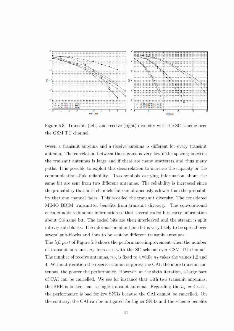
Figure 5.8: Transmit (left) and receive (right) diversity with the SC scheme over

the GSM TU channel.

tween a transmit antenna and a receive antenna is different for every transmit

antenna. The correlation between those gains is very low if the spacing between

the transmit antennas is large and if there are many scatterers and thus many

paths. It is possible to exploit this decorrelation to increase the capacity or the

communications-link reliability. Two symbols carrying information about the

same bit are sent from two different antennas. The reliability is increased since

the probability that both channels fade simultaneously is lower than the probabil-

ity that one channel fades. This is called the transmit diversity. The considered

MIMO BICM transmitter benefits from transmit diversity. The convolutional

encoder adds redundant information so that several coded bits carry information

about the same bit. The coded bits are then interleaved and the stream is split

into nT sub-blocks. The information about one bit is very likely to be spread over

several sub-blocks and thus to be sent by different transmit antennas.

The left part of Figure 5.8 shows the performance improvement when the number

of transmit antennas nT increases with the SC scheme over GSM TU channel.

The number of receive antennas, nR, is fixed to 4 while nT takes the values 1,2 and

4. Without iteration the receiver cannot suppress the CAI: the more transmit an-

tennas, the poorer the performance. However, at the sixth iteration, a large part

of CAI can be cancelled. We see for instance that with two transmit antennas,

the BER is better than a single transmit antenna. Regarding the nT = 4 case,

the performance is bad for low SNRs because the CAI cannot be cancelled. On

the contrary, the CAI can be mitigated for higher SNRs and the scheme benefits

41

from transmit diversity: the nT = 2 and nT = 4 curves at iteration 6 cross each

other at an SNR of abut 3 dB. Note that for a fixed SNR, the total transmit-

ted power and the bit rate are proportional to nT . Therefore, adding one more

transmit antenna increases the spectral efficiency with a linear growth of the total

transmitted power instead of the exponential growth that is usually needed.

The right part of Figure 5.8 shows the performance improvement when the num-

ber of receive antennas nR increases. There is only one transmit antenna (nT = 1)

while nR takes the values 1,2 and 4. The performance is dramatically improved

when nR increases. Two reasons can be identified. The first one is the array

gain. If we are able to constructively combine the signals coming from the receive

antennas and if the noises are independent, then each time nR is doubled, the

noise power is doubled too but the useful power of the signal is multiplied by four.

So each time nR is multiplied by two, the SNR increase is 3 dB what is called the

array gain. The second improvement is due to the receive diversity because not

all the receive antennas are likely to fade simultaneously.

Figure 5.9: Frequency diversity with the SC scheme (left) and the OFDM scheme

(right).

Frequency diversity: When the path delays are small with respect to the symbol

period, around the inverse of the bandwidth, the different paths can not be dis-

tinguished by the receiver. In the case, the channel is frequency flat and there is

no ISI. However, when the symbol period decreases, several groups of paths can

be distinguished by the receiver. There is then ISI and the channel is frequency

selective. Despite the ISI, this case offers an advantage. Indeed, if a distinguish-

42

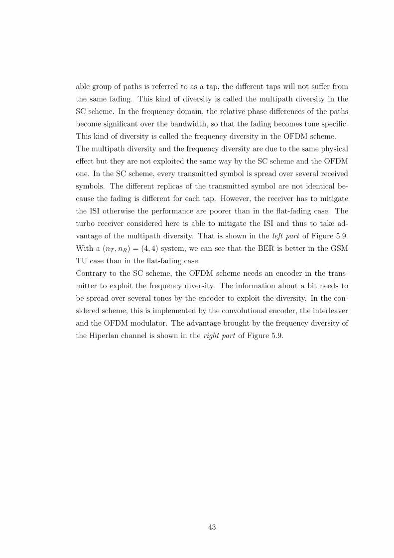
able group of paths is referred to as a tap, the different taps will not suffer from

the same fading. This kind of diversity is called the multipath diversity in the

SC scheme. In the frequency domain, the relative phase differences of the paths

become significant over the bandwidth, so that the fading becomes tone specific.

This kind of diversity is called the frequency diversity in the OFDM scheme.

The multipath diversity and the frequency diversity are due to the same physical

effect but they are not exploited the same way by the SC scheme and the OFDM

one. In the SC scheme, every transmitted symbol is spread over several received

symbols. The different replicas of the transmitted symbol are not identical be-

cause the fading is different for each tap. However, the receiver has to mitigate

the ISI otherwise the performance are poorer than in the flat-fading case. The

turbo receiver considered here is able to mitigate the ISI and thus to take ad-

vantage of the multipath diversity. That is shown in the left part of Figure 5.9.

With a (nT , nR) = (4, 4) system, we can see that the BER is better in the GSM

TU case than in the flat-fading case.

Contrary to the SC scheme, the OFDM scheme needs an encoder in the trans-

mitter to exploit the frequency diversity. The information about a bit needs to

be spread over several tones by the encoder to exploit the diversity. In the con-

sidered scheme, this is implemented by the convolutional encoder, the interleaver

and the OFDM modulator. The advantage brought by the frequency diversity of

the Hiperlan channel is shown in the right part of Figure 5.9.

43

44

Chapter 6

Conclusion

Coding in the signal space is dictated directly by Shannon capacity formula and

suggested by the random coding achievability proof. In early days of digital com-

munications, modulation and coding were kept separated because of complexity.

Modulation and demodulation treated the physical channel, waveform generation,

parameter estimation and symbol-by-symbol detection. Error correcting codes

were used to undo errors introduced by the physical modulation/demodulation

process. This paradigm changed radically with the advent of Coded Modulation.

Trellis-coded modulation was a topic significant research activities in the 80’s, for

approximately a decade. In the early 90’s, new families of powerful random-like

codes, such as turbo-codes and LDPC codes were discovered, along with very effi-

cient low-complexity Belief Propagation iterative decoding algorithms [10] which

allowed unprecedented performance close to capacity, at least for binary-input

channels. Roughly at the same time, bit-interleaved coded modulation emerged

as a very simple yet powerful tool to concatenate virtually any binary code to any

modulation constellation, with only minor penalty with respect to the traditional

joint modulation and decoding paradigm. Therefore, BICM and modern powerful

codes with iterative decoding were a natural marriage, and today virtually any

modern telecommunication system that seeks high spectral efficiency and high

performance, including DSL, digital TV and audio-broadcasting, wireless LANs,

WiMax, and next generation cellular systems use BICM as the central component

of their respective physical layers.

In the first part of the thesis the main theme is that on some channels the sep-

aration of demodulation and decoding might be beneficial, provided that the

45

encoder output is interleaved bitwise and a suitable soft-decision metric is used

in the Viterbi decoder. A comprehensive analysis of BICM, based on BER, shows

this. Optimum and simpler, sub-optimum bit metrics are derived for channels

with state information at the receiver. The central role of labelling map is also

pinpointed.

After that, I have presented a generalized method for analysing the performance

of BICM transmission. Its key element is a new approximation of the pdf of the

bitwise reliability metrics, which is a valuable contribution in its own right. This

approximation has led to closed-form expressions for Laplace transform of pdf,

in term of which BER and cutoff rate of BICM can be expressed. Notably, the

results are applicable to BICM with arbitrary QAM and PSK constellations and

labelling rules, and transmission over Nakagami-m fading channels for arbitrary

m. Furthermore, it was developed an asymptotic analysis which provides valuable

insights into the performance of BICM over fading channels namely expressions

for diversity order and asymptotic coding gain. Selected numerical results have

confirmed the accuracy of the proposed analytical results for SNR regions of in-

terest for convolutional coded BICM.

Then I have reviewed iterative decoding of BICM. In particular I have proved

that BICM-ID significantly outperforms conventional BICM and this makes it

suitable for both AWGN and Rayleigh fading channels.

In conclusion, reporting some applications for BICM, I have shown that in the real

systems this pragmatic approach outperforms a lot of situations, overall where the

old kind of systems are difficult to implement, and where is more constructively

the use of new codes, as turbo-codes.

46

Appendix A

Viterbi Algorithm

The Viterbi algorithm (VA) is a dynamic programming algorithm for finding

the most likely sequence of hidden states - called the Viterbi path - that results

in a sequence of observed events. This algorithm is widely used for estimation

and detection problems in digital communications and signal processing. It is

used to detect signals in communication channels with memory, and to decode

sequential error-control codes that are used to enhance the performance of digital

communication systems [19]. In this appendix I explain the basics of the Viterbi

algorithm as applied to digital communication systems.

Given a received sequence of symbols corrupted by AWGN, the VA finds the

sequence of symbols in the given trellis that is closest in distance to the received

sequence of noisy symbols. This sequence computed is the global most likely

sequence. When Euclidean distance is used as a distance measure, the VA is

the optimal maximum-likelihood detection method in AWGN. The use of this

algorithm in this case is focused on the convolutional codes (Figure A.1), for which

exists two way of decision decoding at the Viterbi decoder; one using Hamming

distance (hard decision decoding) and the other using Euclidean distance (soft

decision decoding). I consider here the second one [20].

To keep the information contained in the received noisy symbols, soft decision

decoding computes the branch metrics by using the noisy symbols directly instead

of quantizing them into bits. For each noisy symbol in the sequence, it calculates

the squared distance between each noisy symbol and the corresponding coded bit

in the coded bit sequence of the given transition, and then adds these distances

together to form the branch metric of the transition. That is, if the given noisy

47

Figure A.1: An example 4-state convolutional code of a rate 1/2.

symbol is x and the coded bits are represented by a and b, then the distance

to coded bits are (x− a)2 and (x− b)2, respectively. For a commonly used rate

k/n convolutional code with binary output symbols represented by, say −a and

a, one can use negation operations to compute the metric for each bit [20]. Since

there are n bits in the output (or coded) bit sequence of each transition, n noisy

symbols are received at the input of the Viterbi decoder at each recursion. Thus,

n negation operations are required to find the metric of all the received symbols

and (n− 1) additions are required to compute the branch metric for a given coded

bit sequence. Therefore, if m is the number of distinct coded bit sequences in the

given trellis, at most M(n−1) additions and n negations are required to compute

the branch metrics for all the transitions and m memory locations are required

to store these branch metrics.

48

Appendix B

Turbo-code

Forward-error-correcting (FEC) channel codes are commonly used to improve the

energy efficiency of wireless communication systems. On the transmitter side, an

FEC encoder adds redundancy to the data in the form of parity information.

Then at the receiver, a FEC decoder is able to exploit the redundancy in such a

way that a reasonable number of channel errors can be corrected. Because more

channel errors can be tolerated with than without an FEC code, coded systems

can afford to operate with a lower transmit power, transmit over longer distances,

tolerate more interference, use smaller antennas, and transmit at a higher data

rate. A binary FEC encoder takes in k bits at a time and produces an output

(or code word) of n bits, where n > k. While there are 2n possible sequences

of n bits, only a small subset of them, 2k to be exact, will be valid code words.

The ratio k/n is called the code rate and is denoted by r. Lower rate codes,

characterized by small values of r, can generally correct more channel errors

than higher rate codes and are thus more energy efficient. However, higher rate

codes are more bandwidth efficient than lower rate codes because the amount of

overhead (in the form of parity bits) is lower. Thus the selection of the code rate

involves a trade-off between energy efficiency and bandwidth efficiency. For every

combination of code rate r, code word length n, modulation format, channel type,

and received noise, there is a theoretic lower limit on the amount of energy that

must be expended to convey one bit of information. This limit is called channel

capacity or Shannon capacity. Since the dawn of information theory, engineers

and mathematicians have tried to construct codes that achieve performance close

to Shannon capacity.

49

The major advancement in coding theory occurred when a group of researchers

developed turbo codes. The initial results showed that turbo codes could achieve

energy efficiencies within only a half decibel of the Shannon capacity. After the

research focused on improving the practicality of turbo codes, which have some

peculiarities that make implementation less than straightforward.

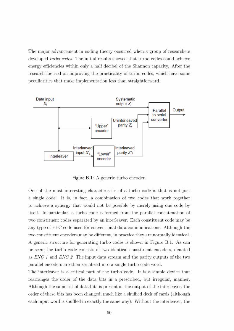
Figure B.1: A generic turbo encoder.

One of the most interesting characteristics of a turbo code is that is not just

a single code. It is, in fact, a combination of two codes that work together

to achieve a synergy that would not be possible by merely using one code by

itself. In particular, a turbo code is formed from the parallel concatenation of

two constituent codes separated by an interleaver. Each constituent code may be

any type of FEC code used for conventional data communications. Although the

two constituent encoders may be different, in practice they are normally identical.

A generic structure for generating turbo codes is shown in Figure B.1. As can

be seen, the turbo code consists of two identical constituent encoders, denoted

as ENC 1 and ENC 2. The input data stream and the parity outputs of the two

parallel encoders are then serialized into a single turbo code word.

The interleaver is a critical part of the turbo code. It is a simple device that

rearranges the order of the data bits in a prescribed, but irregular, manner.

Although the same set of data bits is present at the output of the interleaver, the

order of these bits has been changed, much like a shuffled deck of cards (although

each input word is shuffled in exactly the same way). Without the interleaver, the

50

two constituent encoders would receive the data in the exact same order and thus -

assuming identical constituent encoders - their outputs would be the same. This

would not make for a very interesting (or powerful) code. However, by using

an interleaver, the data Xi is rearranged so that the second encoder receives

it in a different order, denoted X ′i . Thus the output of the second encoder

will almost surely be different than the output of the first encoder - except in

the rare case that the data looks exactly the same after it passes through the

interleaver. Note that the interleaver used by a turbo code is quite different than

the rectangular interleavers that are commonly used in wireless systems to help

break up deep fades. While a rectangular channel interleaver tries to space the

data out according to a regular patter, a turbo code interleaver tries to randomize

the ordering of the data in an irregular manner.

51

Bibliography

[1] C.E. Shannon, A Mathematical Theory on Communication, Bell System

Technical Journal, vol. 27, pp. 379-423 and 623-656, 1948.

[2] G. Ungerboeck, Channel coding with multilevel/phase signal, IEEE Transac-

tions on Information Theory, vol. 28, pp. 55-67, 1982.

[3] E. Zehavi, 8-PSK trellis codes for Rayleigh channel, IEEE Transactions on

Communications, vol. 40, no. 5, pp. 873-884, 1992.

[4] G. Caire, G. Taricco, and E. Biglieri, Bit-interleaved coded modulation, IEEE

Transactions on Information Theory, vol. 44, no. 3, pp. 927-946, 1998.

[5] S. H. Jamali and T. Le-Ngoc, Coded-Modulation Techniques for Fading

Channels, Kluwer Academic Publishers, Boston, Mass, USA, 1994.

[6] E. Biglieri, G. Caire, G. Taricco,J. Ventura-Traveset, Computing Error Prob-

abilities over Fading Channels: a Unified Approach,European Transactions

on Telecommunications, vol. 9, no. 1, pp. 15-25, 1998.

[7] A. Kenarsari Anhari and L. Lampe, An Analytical Approach for Performance

Evaluation of BICM Transmission over Nakagami-m Fading Channels, IEEE

Transactions on Communications, vol. 58, no. 4, pp. 1090-1101, 2010.

[8] X. Li and J. A. Ritcey, Bit-interleaved coded modulation with iterative de-

coding, IEEE Communication Letters, vol. 1, pp. 169-171, 1997.

[9] X. Li and J. A. Ritcey, Trellis-code modulation with bit interleaving and

iterative decoding, IEEE Journal on Selected Areas in Communications, vol.

17, no. 4, pp. 715-724, 1999.

52

[10] A. G. i Fabregas, A. Martinez and G. Caire, Bit-Interleaved Coded Modula-

tion, Foundations and Trends in Communications and Information Theory:

Vol. 5: No 1-2, pp. 1-153, 2008.

[11] J. G. Proakis, Digital Communications, McGraw-Hill USA, 4th edition, 2001.

[12] A. Guillen i Fabregas and G. Caire, Capacity approaching codes for non-

coherent orthogonal modulation, IEEE Transaction Wireless Communica-

tions, vol. 6, pp. 4004-4013, 2007.

[13] E. Biglieri, G. Caire and G. Taricco, Error probability over fading channels.

a unified approach, European Transactions on Communications, 1998.

[14] A. Guillen i Fabregas and G. Caire, Coded modulation in the block-fading

channel: Coding theorems and code construction, IEEE Transactions on In-

formation Theory, vol. 52, pp. 91-114, 2006.

[15] E. Malkamaki and H. Leib, Evaluating the performance of convolutional

codes over block fading channels, IEEE Transactions on Information The-

ory, vol. 45, no.5, pp. 1643-1646, 1999.

[16] L.R. Bahl, J. Cocke, F. Jelinek and J. Raviv, Optimal decoding of linear

codes for minimizing symbol error rate, IEEE Transactions on Information

Theory, vol. 20, pp. 284-287, 1974.

[17] X. Wang, H.V. Poor, Iterative (Turbo) soft interference cancellation and

decoding for coded CDMA, IEEE Transactions on Communications, vol. 47,

pp. 1046-1061, 1999.

[18] X. Wautelet, D. Zuyderhoff and L. Vandendorpe, Bit-interleaved coded mod-

ulation in MIMO systems, communications and Remote Sensing Laboratory,

Universite catholique de Louvain, Belgium, paper.

[19] G. D. Forney Jr., The Viterbi Algorithm, IEEE Proceedings, vol. 61, no. 3,

pp. 268-278, 1973.

[20] H. Lou, Implementing the Viterbi Algorithm, IEEE Signal Processing Mag-

azine, pp. 42-52, 1995.

53

[21] M. Abramowitz and I.A. Stegun, Handbook of mathematical functions, Dover

Publications, 1964.

[22] E. Biglieri, J. Proakis and S. Shamani, Fading channels: information-

theoretic and communications aspects, IEEE Transactions on Information

Theory, vol. 44, no. 6, pp. 2619-2691, 1998.

[23] R.W. Butler, Saddlepoint Approximations with Applications, Cambridge

University Press, 2007.

[24] A. Guillen i Fabregas and A. Grant, Capacity approaching codes for non-

coherent orthogonal modulation, IEEE Transactions on Wireless Communi-

cations, vol. 6, pp. 4004-4013, 2007.

54

AcknowledgementsI miei piu sentiti ringraziamenti vanno alla mia fidanzata Eleonora e a tutti i

componenti della mia la mia famiglia, papa Piergiorgio, mamma Giovanna,

fratello Enrico, che mi hanno accompagnato lungo questo percorso di studi.

Senza di loro tutto cio sarebbe stato impossibile.

Ringrazio inoltre tutte le persone con cui in questi anni ho condiviso la mia

esperienza universitaria, partendo dai compagni di corso Daniele, Andrea,

Davide, Paolo, Alessio, Fabio, Enrico, Damiano, Matteo, Giulio, Viviana e

Francesca, i compagni di studio della biblioteca di Roncade, Giulio, Giovanni,

Gaia, Eleonora, Chiara, Elisa, Marta, Francesca, Mattia e Marcello.

Il piu affettuoso dei ringraziamneti va a tutta la mia compagnia del Parkejo

nella quale ho sempre trovato tutta la serenita, la felicita e il supporto sia

morale che fisico di cui avevo bisogno: Pe, Gero, Sturo, Alessia, Kalta, Bene,

Davide, Erica, Gandi, John B, Cavei, Ivano, Lu, Jim, Nico, Teo, Monia, Monica,

Filtro, Dorothy, Arp, Vale e Valeri.

Come ultimo ma non meno importante (’last but not least’) un ringraziamneto

speciale al mio amico Emanuele con il quale ho trascorso dei fantastici periodi.

GRAZIE MILLE A TUTTI!

Alberto Desidera