Black's Consol Rate Conjecture�

Darrell Du�e1, Jin Ma

2, and Jiongmin Yong

3

Preliminary Draft: July 9, 1993

Abstract. This paper con�rms a version of a conjecture by Fischer Black regarding consol

rate models for the term structure of interest rates. A consol rate model is one in which

the stochastic behavior of the short rate is in uenced by the consol rate. Since the consol

rate is itself determined, via the usual discounted present value formula, by the short rate,

such models have an inherent �xed point aspect.

Under an equivalent martingale measure, purely technical regularity conditions are

given for the stochastic di�erential equation de�ning the short rate and the consol rate to

be consistent with the de�nition of the consol rate as the yield on a perpetual annuity.

The results are based on an extension of the theory for the forward-backward stochastic

di�erential equations to in�nite-horizon settings. Under additional compatibility condi-

tions, we also show that the consol rate is uniquely determined, and given as a function of

the short rate.

�We are grateful for many conversations with Fischer Black, who should not be held

responsible for our interpretation of his conjecture. We are also grateful to the IMA

for supporting our stay at a workshop at which this research was conceived. Some

helpful discussions with P. Protter of Purdue University, A. Conze (formerly of

Goldman Sachs), B. Hu of Notre Dame University and M. V. Safonov of

The University of Minnesota also deserve acknowledgement.

1The Graduate School of Business, Stanford University, Stanford, CA 94305-5015,

partially supported under a grant from the U.S. National Science Foundation,

NSF SES 90-10062.

2Department of Mathematics, Purdue University, West Lafayette, IN 47907-1395,

partially supported by NSF grant # DMS-9301516.

3IMA, University of Minnesota, Minneapolis, MN 55455; on leave from Department

of Mathematics, Fudan University, Shanghai 200433, China. This author is partially

supported by NSF of China and Fok Ying Tung Education Foundation.

1

x1. Introduction

The main objective of this paper is to con�rm and explore a conjecture by Fischer

Black regarding consol rate models for the term structure of interest rates. A consol rate

model is one in which the stochastic behavior of the short rate is in uenced by the consol

rate. Since the consol rate is itself determined, via the usual discounted present value

formula, by the short rate, such models have an inherent �xed-point aspect.

Under purely technical conditions, we show whether or not a stochastic di�erential

equation de�ning the short rate and the consol rate is consistent with the de�nition of the

consol rate as the yield on a perpetual annuity. The results are based on an extension

of the theory for the forward-backward stochastic di�erential equations to in�nite-horizon

settings.

We �x a �ltered probability space (;F ; P ; fFtgt�0), satisfying the usual conditions.

(See, for example, Protter (1990) for background technical de�nitions.) A consol is a

perpetual annuity, that is, a security paying dividends continually and in perpetuity at a

constant rate, which can be taken without loss of generality to be 1. A short rate process

is a non-negative progressively measurable process. We are interested in models of a short

rate process r and a price process Y for the consol that satisfy the expected discounted

value formula

(1:1) Yt = E

�Z1

t

exp

��

Z s

t

ru du

�ds

���� Ft�; t � 0;

where E denotes expectation under P . Without getting into the associated de�nitions

and related notions of arbitrage, (1.1) is consistent with the role of P as an \equivalent

martingale measure," in the sense of Harrison and Kreps (1979), which can be consulted for

the associated theory. It is not unusual in applications to work from the beginning under

such a probability measure, and we do so. Since the yield on a consol is the reciprocal of

its price, and since reciprocation is a smooth mapping from (0;1) to (0;1) with a smooth

inverse, it makes no di�erence whether we work in terms of the price process Y or its yield

process ` = Y �1, also known as the consol rate process.

Since the work of Brennan and Schwartz (1979), there has been interest in term-

structure models based on a stochastic di�erential equation for the short rate r and the

2

consol rate `. Since Y = `�1, we can equally well work in terms of a stochastic di�erential

equation for (r; Y ) of the form

drt =�(rt; Yt) dt+ �(rt; Yt) dWt(1:2)

dYt =(rtYt � 1) dt+A(rt; Yt) dWt;(1:3)

where W is a standard Brownian motion in lR2, and where �, �, and A are measurable

functions on (0;1) � (0;1) into lR, lR2; and lR

2, respectively, satisfying technical condi-

tions. The drift rtYt � 1 shown for Y is implied directly by (1.1) and Ito's formula, and

is interpreted as a statement that the expected rate of return on the consol (under the

measure P ) is the short (riskless) rate r.

Our �rst objective is to show how to determine whether the di�usion function A on the

consol price process is consistent with the characterization (1.1) of the consol price. It is

clear that not any choice for A will work. For example, we cannot have a(r; y)>A(r; y) = 0

for all (r; y), unless both a and A are identically zero, since the increments of r and Y

must be correlated in a very particular fashion, given the de�nition (1.1) of Y . Indeed, we

want to resolve whether any A can be chosen in a manner consistent with (1.1). Since Yt

depends on the conditional distribution of frs : s � tg, which in turn depends at least on

� and � (not to mention the dependence of r, through Y , on A itself), we should expect

that the di�usion function A for Y depends in a particular way on � and �.

In a private communication, Black has conjectured that, under at most technical con-

ditions, for any (�;�) there is always a choice for A that works. We con�rm that conjecture.

We also provide additional technical conditions under which (1.2)-(1.3) is consistent with

(1.1) if and only if Yt = '(rt) and (consequently) A(rt; Yt) = '0(rt)�(rt; '(rt)); where '

is a C2solution of the ordinary di�erential equation

(1:4) '0(x)�(x;'(x)) � x'(x) +1

2

'00(x)k�(x;'(x))k2 + 1 = 0; x 2 (0;1):

Under the same technical conditions, there is a unique solution to this ordinary di�erential

equation. This result, connecting the ODE (1.4) with solutions to the model (1.1){(1.3)

of short rate and consol rate, is based on recent developments in the theory of forward-

backward stochastic di�erential equations reported in Ma and Yong (1993) and Ma, Prot-

ter, and Yong (1993).

3

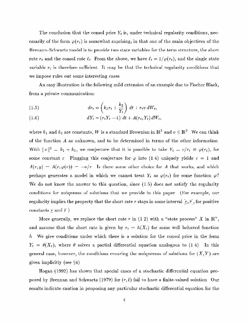
The conclusion that the consol price Yt is, under technical regularity conditions, nec-

essarily of the form '(rt) is somewhat suprising, in that one of the main objectives of the

Brenann-Schwartz model is to provide two state variables for the term structure, the short

rate rt and the consol rate `t. From the above, we have `t = 1='(rt), and the single state

variable rt is therefore su�cient. It may be that the technical regularity conditions that

we impose rules out some interesting cases.

An easy illustration is the following mild extension of an example due to Fischer Black,

from a private communication:

drt =

�k1rt +

k2

Yt

�dt+ rtv dWt;(1:5)

dYt =(rtYt � 1) dt+A(rt; Yt) dWt;(1:6)

where k1 and k2 are constants,W is a standard Brownian in lR2and v 2 lR

2. We can think

of the function A as unknown, and to be determined in terms of the other information.

With kvk2 = k1 + k2, we conjecture that it is possible to take Yt = c=rt � '(rt), for

some constant c. Plugging this conjecture for ' into (1.4) uniquely yields c = 1 and

A(r; y) = A(r; '(r)) = �v=r. Is there some other choice for A that works, and which

perhaps generates a model in which we cannot treat Yt as '(rt) for some function '?

We do not know the answer to this question, since (1.5) does not satisfy the regularity

conditions for uniquness of solutions that we provide in this paper. (For example, our

regularity implies the property that the short rate r stays in some interval [r; r]; for positive

constants r and r.)

More generally, we replace the short rate r in (1.2) with a \state process" X in lRn,

and assume that the short rate is given by rt = h(Xt) for some well behaved function

h. We give conditions under which there is a solution for the consol price in the form

Yt = �(Xt), where � solves a partial di�erential equation analogous to (1.4). In this

general case, however, the conditions ensuring the uniqueness of solutions for (X;Y ) are

given implicitly (see x4).

Hogan (1992) has shown that special cases of a stochastic di�erential equation pro-

posed by Brennan and Schwartz (1979) for (r; `) fail to have a �nite-valued solution. Our

results indicate caution in proposing any particular stochastic di�erential equation for the

4

short rate and consol rate, whether or not it has a �nite solution, if the consol rate is in-

tended to represent the yield on a consol in a manner consistent with the proposed model.

The di�usion of the consol must be chosen consistently with the solution of a non-trivial

�xed point problem involving the drift and di�usion of the short rate.

One could also apply our results to a general class of �nancial market valuation prob-

lems. Suppose, for instance, that one wants to develop a model in which the stochastic

behavior of the state process is in uenced in a particular way by certain asset prices, which

are in turn determined by the usual discounted expected valuation approach, with future

state prices given in terms of future state variables. We show how this can be done con-

sistently, and give a di�erential equation for the asset price in terms of the state variables.

In the in�nite-horizon setting, uniqueness is shown under somewhat narrower su�cient

conditions.

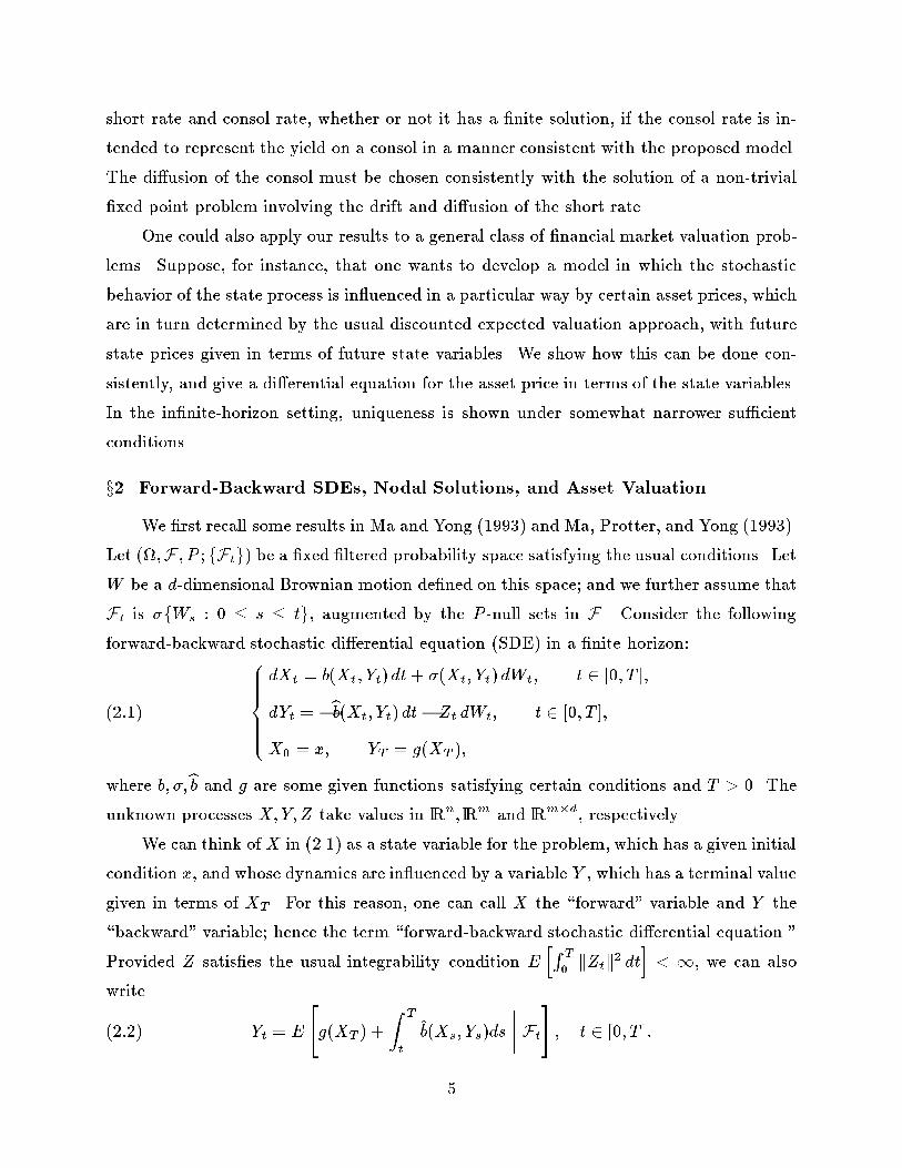
x2. Forward-Backward SDEs, Nodal Solutions, and Asset Valuation

We �rst recall some results in Ma and Yong (1993) and Ma, Protter, and Yong (1993).

Let (;F ; P ; fFtg) be a �xed �ltered probability space satisfying the usual conditions. Let

W be a d-dimensional Brownian motion de�ned on this space; and we further assume that

Ft is �fWs : 0 � s � tg, augmented by the P -null sets in F . Consider the following

forward-backward stochastic di�erential equation (SDE) in a �nite horizon:

(2:1)

8>>><>>>:dXt = b(Xt; Yt) dt + �(Xt; Yt) dWt; t 2 [0; T ];

dYt = �bb(Xt; Yt) dt� Zt dWt; t 2 [0; T ];

X0 = x; YT = g(XT );

where b; �;bb and g are some given functions satisfying certain conditions and T > 0. The

unknown processes X;Y;Z take values in lRn; lRm

and lRm�d

, respectively.

We can think of X in (2.1) as a state variable for the problem, which has a given initial

condition x, and whose dynamics are in uenced by a variable Y , which has a terminal value

given in terms of XT . For this reason, one can call X the \forward" variable and Y the

\backward" variable; hence the term \forward-backward stochastic di�erential equation."

Provided Z satis�es the usual integrability condition EhR T

0kZtk

2 dti< 1, we can also

write

(2:2) Yt = E

"g(XT ) +

Z T

t

b(Xs; Ys)ds

���� Ft#; t 2 [0; T ]:

5

In all of our applications in this paper, Y will turn out to be a vector of prices of certain

�nancial securities, while X is a state variable that a�ects both the dynamics and the �nal

value of Y . Determining a solution for (X;Y ) may be thought of as �xed point problem.

In other applications, such as models of recursive utility, we may think of Yt as the vector

of current utilities of the various economic agents in a given Pareto problem, as in Epstein

(1987) (deterministic case) or Du�e, Geo�ard, and Skiadas (1992) (stochastic case). In

that problem, we may think of X as determined by the aggregate consumption process

and the vector of utility weights. In general, we use the following de�nition.

De�nition 2.1. A process (X;Y;Z) is called an adapted solution of (2.1) if it is fFtg-

adapted, square-integrable and satis�es

(2:3)

8>>><>>>:Xt = x +

Z t

0

b(Xs; Ys) ds +

Z t

0

�(Xs; Ys) dWs;

Yt = g(XT ) +

Z T

t

bb(Xs; Ys) ds +

Z T

t

Zs dWs;

t 2 [0; T ]:

Moreover, if there exists a function � : lRn � [0; T ] ! lRm, which is C1

i n t and C2in x,

such that the adapted solution (X;Y;Z) satis�es

(2:4) Yt = �(Xt; t); Zt = ��(Xt; �(Xt; t))>�x(Xt; t); t � 0;

then (X;Y;Z) is called a nodal solution of (2.1).

We use the term \nodal solution" because � in some cases turns out to be the \nodal

surface" of the viscosity solution to a certain Hamilton-Jacobi-Bellman equation (see Ma

and Yong (1993) for details). From Ma, Yong, and Protter (1993), we know that under

certain conditions, any adapted solution of (2.1) must be a nodal solution. Moreover, the

nodal solution is unique. As a matter of fact, this nodal solution can be constructed by

the following way: First, �nd the unique classical solution � of the parabolic system:

(2:5)

8>>><>>>:�kt +

1

2

tr (�kxx�(x; �)�(x; �)>) + h b(x; �); �kx i+

bbk(x; �) = 0;

(t; x) 2 (0; T ) � lRn; 1 � k � m;

�(T; x) = g(x); x 2 lRn:

6

Second, solve the forward SDE:

(2:6)

(dXt = b(Xt; �(Xt; t)) dt + �(Xt; �(Xt; t)) dWt; t 2 [0; T ];

X0 = x:

Finally, set Yt and Zt as in (2.4). This will give the nodal solution of (2.1). Such a method

was called a \Four Step Scheme" in [Ma, Protter and Yong (1993)], where more general

cases were studied.

In what follows, we restrict ourselves to the case m = 1 and

(2:7) bb(x; y) = 1� h(x)y; (x; y) 2 lRn � lR;

for some function h : lRn ! (0;1). Then, (2.1) becomes

(2:8)

8>>><>>>:dXt = b(Xt; Yt) dt + �(Xt; Yt) dWt; t 2 [0; T ];

dYt = (h(Xt)Yt � 1) dt � hZt; dWt i; t 2 [0; T ];

X0 = x; YT = g(XT );

By the usual variation of constant formula, we have

(2:9)

g(XT ) = YT = e

RT

th(Xu)duYt �

Z T

t

e

RT

sh(Xu)du ds

�

Z T

t

e

RT

sh(Xu)du hZs; dWs i; t 2 [0; T ]:

This implies that

(2:10)

Yt = e�

RT

th(Xu)dug(XT ) +

Z T

t

e�

Rs

th(Xu)duds

+

Z T

t

e�

Rs

th(Xu) du hZs; dWs i; t 2 [0; T ]:

Taking conditional expectations and noting that

RhZ; dW i is a martingale (as is the case

under the square-integrable condition on Z), we obtain

(2:11) Yt = E

"e�

RT

th(Xu)dug(XT ) +

Z T

t

e�

Rs

th(Xu)du ds

��� Ft#; t 2 [0; T ]:

Hence, it is expected that (2.8) should be very closely related to the following problem,

which we call the Finite-Horizon Valuation Problem:

7

Problem FHVR. Find an adapted process (X;Y ) such that

(2:12)

8><>:dXt = b(Xt; Yt) dt + �(Xt; Yt) dWt; t 2 [0; T ]; X0 = x;

Yt = E

"e�

RT

th(Xu) dug(XT ) +

Z T

t

e�

Rs

th(Xu) du ds

��� Ft#; t 2 [0; T ]:

In the problem FHVR (2.12), treating rt = h(Xt) as the short rate of interest in a

�nance setting, we may think of Y as the price of a security claiming a continual constant

unit dividend until time T , at which time the security is valued at g(XT ). The unusual

aspect of this formulation, relative to the typical model, is that the state process X has

dynamics that depend on the price process Y , while Yt itself depends on the conditional

distribution of Xs for s � t. If we take g � 0, we have a �nite horizon annuity valuation

problem, in which the annuity price in uences the short rate. The consol rate problem is

the in�nite-horizon version of this problem. We will show technical conditions (Proposition

3.1) under which Yt = �(Xt; t) for some unique function �, so that there is no role for Y as

a separate state variable. Later, under additional regularity, we will show that this is also

true in the in�nite-horizon setting (Section 4) for some time-independent �, and that the

�nite-horizon solutions will converge to the in�nite-horizon solution as the horizon T !1

(Section 5).

Any adapted process (X;Y ) satisfying (2.11) is called an adapted solution of Problem

FHVR. Moreover, we have the following notion.

De�nition 2.2. An adapted solution (X;Y ) of Problem FHVR is called a nodal solution

of Problem FHVR if there exists a function � : lRn � [0; T ]! lR, which is C1in t and C2

in x, such that

(2:13) Yt = �(Xt; t); t 2 [0; T ]:

We will call (2.8) the forward-backward SDE associated with Problem FHVR.

The main purpose of this paper is to study the following problem, which is called the

In�nite-Horizon Consol Rate Problem in the sequel.

Problem IHCR. Find an adapted, locally square-integrable process (X;Y ), such that

(2:14)

8><>:dXt = b(Xt; Yt) dt+ �(Xt; Yt) dWt; t 2 [0;1); X0 = x;

Yt = E

�Z1

t

e�

Rs

th(Xu)duds

��� Ft�; t 2 [0;1):

8

Any adapted process (X;Y ) satisfying (2.14) is called an adapted solution of Problem

IHCR. Moreover, we have the following de�nition similar to De�nition 2.2.

De�nition 2.3. An adapted solution (X;Y ) of Problem IHCR is called a nodal solution

of Problem IHCR if there exists a bounded C2function � with �x being bounded, such

that

(2:15) Yt = �(Xt); t 2 [0;1):

We note that in De�nition 2.3, the function � is time-independent because of the

in�nite horizon. Formally, the forward-backward SDE associated with Problem IHCR is

the following:

(2:16)

8>>>>>><>>>>>>:

dXt = b(Xt; Yt) dt + �(Xt; Yt) dWt; t 2 [0;1);

dYt = (h(Xt)Yt � 1) dt� hZt; dWt i; t 2 [0;1);

X0 = x;

Yt is bounded a.s. ; uniformly in t 2 [0;1):

We shall verify this in the next section. Also, we should note that, in general, the asymp-

totic behavior of Yt at t = 1 is not known, we therefore only impose the boundedness of

Y instead. As before, we may introduce the following de�nition.

De�nition 2.4. A process (X;Y;Z) is called an adapted solution of (2.16) if it is fFtg-

adapted, locally square-integrable, and if

(2:17)

8>>><>>>:Xt = x+

Z t

0

b(Xs; Ys) ds +

Z t

0

�(Xs; Ys) dWs; t 2 [0;1);

Yt = Yu +

Z t

u

[h(Xs)Ys � 1] ds �

Z t

u

hZs; dWs i; 0 � u � t <1:

Moreover, if there exists a bounded C2function � with �x being bounded, such that the

adapted solution (X;Y;Z) has the following relations:

(2:18) Yt = �(Xt); Zt = ��(Xt; �(Xt))>�x(Xt); t 2 [0;1);

then, we call (X;Y;Z) a nodal solution of (2.16).

9

x3. Existence of Nodal Solutions

In this section we study the existence of nodal solutions to both Problem FHVR and

Problem IHCR. We shall also establish the relationship between these problems and the

associated forward-backward SDEs, and some properties of the nodal solutions. Let us

�rst make some Standing Assumptions.

(H1) The functions �; b; h are C1with bounded partial derivatives and there exist

constants �; � > 0, and some continuous increasing function � : [0;1)! [0;1), such that

(3:1) �I � �(x; y)�(x; y)> � �I; (x; y) 2 lRn � lR;

(3:2) jb(x; y)j � �(jyj); (x; y) 2 lRn � lR;

(3:3) infx2lRn

h(x) � � > 0; sup

x2lRnh(x) � <1:

(H2) The function g is bounded in C2+�(lR

n); for some � > 0.

Let us begin with the Problem FHVR.

Proposition 3.1. Let (H1){(H2) hold. Then, Problem FHVR admits a unique adapted

solution (X;Y ). Moreover, it is in fact a nodal solution.

Proof. First, from the previous section, we see that if (X;Y;Z) is an adapted solution of

(2.8), then (X;Y ) is an adapted solution of Problem FHVR. Conversely, let (X;Y ) be any

adapted solution of Problem FHVR. We shall prove that there exists an adapted lRd-valued

process Z such that (X;Y;Z) is an adapted solution to (2.8).

To this end, let us de�ne a measurable process

(3:4) Ut�

= e�

RT

th(Xu)dug(XT ) +

Z T

t

e�

Rs

th(Xu)du ds:

Clearly, for each t 2 [0; T ], Ut is FT -measurable. Let Yt�

=E[UtjFt], t 2 [0; T ]. Then note

that the Brownian �ltration fFtg is actually continuous (cf. Karatzas and Shreve (1988)),

10

Y is continuous and is indistinguishable from the optional (or predictable) projection of

U . Furthermore, it holds that

(3:5) E

"Z T

t

HsUs ds���Ft#= E

"Z T

t

HsYsds���Ft#;

for any t 2 [0; T ], P -a.s. ; where H is any bounded, fFtg-adapted process (see, for example

Dellacherie and Meyer (1982), VI).

On the other hand, for each �xed ! 2 , one can check by direct computation that

U satis�es the ODE:

(3:6) Ut(!) = g(XT (!)) +

Z T

t

(h(Xs(!))Us(!) � 1)ds:

Taking conditional expectation on both sides of (3.6) and applying (3.5), we see that Yt

satis�es

(3:7) Yt = Ehg(XT ) +

Z T

t

(h(Xs)Ys � 1) ds���Fti;

P -almost surely. Now by applying the martingale representation theorem and following the

argument as that in Ma, Protter and Yong (1993), x5 (note the boundedness of g, h, and

the adaptedness of Y ), we see that there exists an adapted, lRd-valued, square-integrable

process fZt : 0 � t � Tg, such that

(3:8) Yt = g(XT ) +

Z T

t

(h(Xs)Ys � 1) ds �

Z T

t

hZs; dWs i :

In other words, (X;Y;Z) solves (2.8). (In some �nance applications, the Brownian motion

W does not generate the given �ltration fFtg; as assumed in this paper, but rather is

obtained as the martingale part of a Brownian motion under a di�erent measure, via

Girsanov's Theorem. Even in this more general setting, it can be seen that W generates

all martingales as stochastic integrals in the above sense.)

Finally, since the process Y is one dimensional, the results in Ma, Protter, and Yong

(1993) show that (2.8) posseses a unique adapted solution which can be constructed via

the Four Step Scheme; namely, any adapted solution of (2.8) must be the nodal solution,

proving the proposition.

11

To study the Problem IHCR, we need the following lemma. The proof of the lemma

is quite standard, but we nevertheless sketch it for the bene�t of the reader.

Lemma 3.2. Let (H1) hold. Then, the following equation admits a classical solution

� 2 C2+�(lR

n):

(3:9)1

2

tr

��xx�(x; �)�

>(x; �)

�+ h b(x; �); �x i�h(x)� + 1 = 0; x 2 lR

n:

Moreover, this solution satis�es

(3:10)1

� �(x) �

1

�; x 2 lR

n:

Sketch of the proof. Let BR(0) be the ball of radius R > 0 centered at the origin. We con-

sider the equation (3.9) in BR(0) with the homogeneous Dirichlet boundary condition. By

Gilbarg and Trudinger (1977), Theorem 14.10, there exists a solution �R 2 C2+�(BR(0))

for some � > 0. By the maximum principle, we have

(3:11) 0 � �R(x) �1

�; x 2 BR(0):

Next, for any �xed x0 2 lRn, and R > jx0j+ 2, by Gilbarg and Trudinger, Theorem 14.6,

we have

(3:12) j�Rx (x)j � C; x 2 B1(x0);

where the constant C is independent ofR > jx0j+2. This, together with the boundedness of

� and the �rst partial derivatives of �; b; h, implies that as a linear equation in � (regarding

�(x; �(x)) and b(x; �(x)) as known functions), the coe�cients are bounded in C1. Hence,

by Schauder's interior estimates, we obtain that

(3:13) k�RkC2+�(B1(x0)) � C; R > jx0j+ 2:

Then, we can let R!1 along some sequence to get a limit function �(x). By the standard

diagonalization argument, we may assume that � is de�ned in the whole of lRn. Clearly,

� 2 C2+�(lR

n) and is a classical solution of (3.9). Finally, by the maximumprinciple again,

we obtain (3.10).

12

Now, we come up with the following existence result for the Problem IHCR.

Theorem 3.3. Let (H1) hold. Then, there exists at least one nodal solution (X;Y ) of

Problem IHCR.

Proof. By Lemma 3.2, we can �nd a classical solution � 2 C2+�(lR

n) of (3.9). Now, we

consider the following (forward) SDE:

(3:14)

(dXt = b(Xt; �(Xt)) dt + �(Xt; �(Xt)) dWt; t > 0;

X0 = x:

Since �x is bounded and b and � are uniformly Lipschitz, (3.14) admits a unique strong

solution Xt, t 2 [0;1). Next, we de�ne

(3:15) Yt = �(Xt); t 2 [0;1):

We are going to show that (X;Y ) is an adapted solution of Problem IHCR. In fact, by

using Ito's formula, we have

(3:16)

dYt =hh �x(Xt); b(Xt; �(Xt)) i+

1

2

tr

��xx(Xt)�(Xt; �(Xt))�

>(Xt; �(Xt))

�idt

+ h �x(Xt); �(Xt; �(Xt)) dWt i

=

�h(Xt)�(Xt)� 1

�dt+ h �>(Xt; �(Xt))�x(Xt); dWt i

=

�h(Xt)Yt � 1

�dt� hZt; dWt i;

where Zt = ��(Xt; �(Xt))>�x(Xt) and the equation (3.9) has been used. Clearly, (3.16)

can be regarded as a linear non-homogeneous SDE in Yt. Thus, the usual variation of

constants formula gives

(3:17)YT = e

RT

th(Xu)duYt �

Z T

t

e

RT

sh(Xu)du ds +

Z T

t

h e

RT

sh(Xu)duZs; dWs i;

0 � t � T <1:

The above can also be written as

(3:18)Yt = e

�

RT

th(Xu) duYT +

Z T

t

e�

Rs

th(Xu)du ds �

Z T

t

h e�

Rs

th(Xu) duZs; dWs i;

0 � t � T <1:

13

Next, we take the conditional expectations, using the local square-integrability of Z implied

by the properties of � and � to obtain

(3:19) Yt = E

"e�

RT

th(Xu)duYT +

Z T

t

e�

Rs

th(Xu)duds

���Ft#; 0 � t � T <1:

Since � is bounded, so is Y (see (3.15)). Consequently, by condition (3.3),

(3:20)���e�R Tt h(Xr)drYT

��� � 1

�e��(T�t) ! 0; (T !1):

On the other hand, for any T � T 0,

(3:21)

��� Z T 0

T

e�

Rs

th(Xu) du ds

��� � Z T 0

T

e��(s�t) ds = e�te��T � e��T

0

�! 0;

(T; T 0 !1):

Namely, for each �xed (t; !), the integral above converges as T ! 1, hence, by the

Dominated Convergence Theorem, we can send T !1 in (3.19) to get

(3:22) Yt = E

�Z1

t

e�

Rs

th(Xu)du ds

���Ft�; t 2 [0;1):

This shows that (X;Y ) is an adapted solution of Problem IHCR. By (3.15), this solution

is nodal.

Next, we discuss the possibility of representing the solution of Problem IHCR as the

adapted solution of forward-backward SDE (2.16). As was pointed out in the introduction,

in the general in�nite-horizon case, we don't have the uniqueness of the forward-backward

SDE if the value at in�nity cannot be speci�ed. Nevertheless, we shall show below and in

the next section that the uniqueness in the certain class of solutions will still hold, which

will be su�cient for our purpose.

To begin with, let us establish a result concerning the non-autonomous ODE with

in�nite duration. Let H : [0;1) ! [�;1) be a continuous function, where � > 0 is given,

consider the ODE:

(3:23)dUt

dt= HtUt � 1:

We have the following lemma.

14

Lemma 3.4. There exists a unique bounded solution of (3.23) de�ned on [0;1). More-

over, such a solution has an explicit expression:

(3:24) Ut =

Z1

t

e�

Rs

tHudu ds:

Proof. The existence follows from a direct veri�cation that the function U de�ned by

(3.24) is a bounded solution of (3.23). To see the uniqueness, it su�ces to show that any

bounded solution of (3.23) must be of the form (3.24). Indeed, let U be any bounded

solution to (3.23) de�ned on [0;1). For any 0 � t � T , we can apply the variation of

constants formula to get

(3:25) Ut = e�

RT

tHuduUT +

Z T

t

e�

Rs

tHududs:

Since UT is bounded (for all T > 0), we have

(3:26)

���e� R Tt HrdrUT

��� � Ce��(T�t) ! 0; as T ! 0:

Hence a similar argument proving (3.22) shows that (3.24) holds. This proves the lemma.

Proposition 3.5. If (X;Y ) is an adapted solution to Problem IHCR, then there exists an

adapted, lRd-valued, locally square-integrable process Z, such that (X;Y;Z) is an adapted

solution of (2.16).

Proof. Suppose that (X;Y ) is an adapted solution to Problem IHCR. De�ne

(3:27) Ut =

Z1

t

e�

Rs

th(Xu)du ds:

By the assumption on the function h, Ut is well-de�ned for each t � 0. Clearly, Y is the

optional projection of U ; to wit, Yt = E(UtjFt), t � 0.

Now for each �xed ! 2 , de�ne Ht(!) = h(Xt(!)), t � 0. Then t 7! Ht(!) is

continuous and bounded below by � > 0. Therefore, by Lemma 3.4, we see that U is the

unique bounded solution of the ODE (with random coe�cients):

(3:28)dUt

dt= h(Xt)Ut � 1:

15

Now, whenever 0 � t < T <1, we have

(3:29) Ut = UT �

Z T

t

[h(Xs)Us � 1] ds;

whence

(3:30)

Yt = E(UtjFt)

= EhUT �

Z T

t

[h(Xs)Us � 1] ds

���Fti

= EhUT �

Z T

t

[h(Xs)Ys � 1] ds���Fti;

where we have used the fact that Y is the optional projection of U . Thus, a by now

standard argument using the martingale representation theorem, as in the �nite horizon

case, leads to the existence of an adapted, square-integrable process Z(T )de�ned on [0; T ],

such that

(3:31) Yt = UT �

Z T

t

[h(Xs)Ys � 1] ds+

Z T

t

hZ(T )s ; dWs i; t 2 [0; T ]:

It remains to show that there exists an adapted, locally integrable process Z taking values

in lRdsuch that

(3:32)

Z T

t

hZs; dWs i =

Z T

t

hZ(T )s ; dWs i; 0 � t � T <1:

To see this, note that (3.31) holds for any T > 0, so if 0 � T1 < T2 <1, then for t 2 [0; T1],

we have

(3:33)

Yt = UT1 �

Z T1

t

[h(Xs)Ys � 1] ds +

Z T1

t

hZ(T1)s ; dWs i

= UT2 �

Z T2

t

[h(Xs)Ys � 1] ds +

Z T2

t

hZ(T2)s ; dWs i :

Setting t = T1, we get

(3:34) UT1 = UT2 �

Z T2

T1

[h(Xs)Ys � 1] ds+

Z T2

T1

hZ(T2)s ; dWs i :

Plugging (3.34) into (3.33), we obtain that

(3:35)

Z T1

t

hZ(T2)s �Z(T1)

s ; dWs i = 0; for all t 2 [0; T1]:

16

This leads to the property:

(3:36) E

Z T1

0

[Z(T2)s � Z(T1)

]2 ds

!= 0:

In other words, Z(T1)= Z(T2)

, dt dP -almost surely on [0; T1] � . Therefore, modulo a

dt dP -null set, we can de�ne a process Z by Zt = Z(N)

t , if t 2 [0;N ], where N = 1; 2; � � �;

and it is fairly easy to check as before that (3.32) holds. Therefore, (3.31) can be rewriten

as

(3:37) Yt = UT �

Z T

t

[h(Xs)Ys � 1] ds+

Z T

t

hZs; dWs i;

for all T > 0, or equivalently, one has

(3:38) dYt = [h(Xt)Yt � 1] dt� hZt; dWt i; t 2 [0;1):

Finally, the boundedness of Y follows easily from the de�nition of Y and the fact that

Ut �1

�, 8t � 0, P -a.s. ; proving the proposition.

It is worth noting that although the bounded solution U of the random ODE (3.23)

over the in�nite-horizon is unique, the uniqueness of the adapted solution to the forward-

backward SDE (2.16) over an in�nite duration is still unknown. Theorem 3.3 and Proposi-

tion 3.5 suggested two ways to construct the adapted solutions to such forward-backward

SDEs. In the next section we shall prove that if both X and Y are one-dimensional,

then the adapted solution to the forward-backward SDE over an in�nite-horizon is unique,

under some explicit compatibility conditions; and such adapted solutions must be nodal

(see Theorem 4.1). In the higher dimensional case, such a result is also proved (Theorem

4.5), but the condition that we have to pose is implicit; and the general uniqueness result

is far from obvious. Nevertheless, one would expect that the uniqueness should hold at

lease among the nodal solutions. The next result and the remark following it explore its

possibility. Recall from De�nition 2.4 that a nodal solution can be given by an arbitrary

bounded C2function � with bounded gradient.

Proposition 3.6. Let (H1) hold. Suppose that forward-backward SDE (2.16) has a nodal

solution (X;Y;Z); namely, (2.18) holds for some bounded C2 function � with bounded

gradient. Then � must satisfy the ODE (3.9).

17

Proof. Let (2.18) holds for some bounded C2function � with bounded gradient. Since �

is C2, we can apply Ito's formula to Yt = �(Xt). This leads to that

(3:39)dYt =

hh b(Xt; �(Xt)); �x(Xt) i+

1

2

tr

��xx(Xt)��

>(Xt; �(Xt))

�idt

+ h �x(Xt); �(Xt; �(Xt))dWt i :

Comparing (3.39) with (2.16) and noting that Yt = �(Xt), we obtain that

(3:40) h b(Xt; �(Xt)); �x(Xt) i+1

2

tr

��xx(Xt)��

>(Xt; �(Xt))

�= h(Xt)�(Xt)� 1;

for all t � 0, P -almost surely. De�ne a continuous function F : lRn ! lR by

(3:41) F (x)�

= h b(x; �(x)); �x(x) i+1

2

tr

��xx(x)��

>(x; �(x))

�� h(x)�(x) + 1:

We shall prove that F � 0. In fact, note that in this case, X actually satis�es the forward

SDE

(3:42)

8<:dXt =

eb(Xt) dt+ e�(Xt) dWt; t � 0;

X0 = x;

where eb(x) �= b(x; �(x)); e�(x) �=�(x; �(x)). Therefore X is a time-homogeneous Markov

process with some transition probability density p(t; x; y). Since both eb and e� are bounded

and satisfy a Lipschitz condition; and since ��> is uniformly positive de�nite, it is well

known (see, for example, Friedman (1964, 1975)) that for each y 2 lRn, p(�; �; y) is the

fundamental solution of the following parabolic PDE:

(3:43)1

2

nXi;j=1

eaij(x) @2p

@xi@xj+

nXi=1

ebi(x) @p@xi

�@p

@t= 0;

and it is positive everywhere. Now by (3.40), we have that F (Xt) = 0 for all t � 0, P -a.s. ,

whence E0;x[F2(Xt)] = 0, for all t > 0. Since

(3:44) E0;x

�F 2

(Xt)�=

ZlRn

p(t; x; y)F 2(y) dy; t > 0;

and p(t; x; y) is positive everywhere, we have F (y) = 0 almost everywhere under the

Lebesgue measure in lRn. The result then follows from the continuity of F .

18

Remark 3.7. The essence of Proposition 3.6 is that the only possible nodal solution for

the in�nite horizon forward-backward SDE (2.16) is the one constructed using the solution

of ODE (3.9). Therefore, if (3.9) has multiple solutions, we don't have uniqueness of the

nodal solution; and the number of the nodal solutions will be exactly the same as that of

the solutions to (3.9). However, if the solution of (3.9) is unique, then the nodal solution

of (2.16) (or equivalently, Problem IHCR) will be unique as well.

x4. Uniqueness of the Nodal Solution

In this section we study the uniqueness of the nodal solution of Problem IHCR. We

�rst consider the one dimensional case, that is, when X and Y are both one-dimensional

processes. For simplicity, we denote

(4:1) a(x; y) =1

2

k�(x; y)k2; (x; y) 2 lR2:

Let us make the some further assumptions:

(H3) Let m = n = 1 and the functions a; b; h satisfy the following:

(4:2) h is strictly increasing:

(4:3)

8>>>>><>>>>>:

a(x; y)h(x) � (h(x)y � 1)

Z1

0

ay(x; (1 � �)y + �by) d� � � > 0;

Z1

0

ha(x; y)by (x; (1 � �)y + �by)� ay(x; (1 � �)y + �by)b(x; y)i d� � 0;

y; by 2 [1

; 1�]; x 2 lR:

Condition (4.3) essentially says that the coe�cients b; � and h should be somewhat

\compatible." Although a little complicated, it is still quite explicit and easily veri�able.

For example, a su�cient conditions for (4.3) is

(4:4)

(a(x; y)h(x) � (h(x)y � 1)ay(x;w) � � > 0;

a(x; y)by (x;w) � ay(x;w)b(x; y) � 0;y; w 2 [

1

; 1�]; x 2 lR:

It is readily seen that the following will guarantee (4.4):

(4:5) ay(x; y) = 0; by(x; y) � 0; (x; y) 2 lR� [1

; 1�]:

19

In particular, if both a and b are independent of y, then (4.3) holds automatically.

Our main result of this section is the following uniqueness theorem.

Theorem 4.1. Let (H1) and (H3) hold. Then Problem IHCR has a unique adapted

solution. Moreoever, this solution is nodal.

To prove the above result, we need the following lemmas.

Lemma 4.2. Let h be strictly increasing and � solve

(4:6) a(x; �)�xx + b(x; �)�x � h(x)� + 1 = 0; x 2 lR:

Suppose xM is a local maximum of � and xm is a local minimum of � with �(xm) � �(xM ).

Then, xm > xM .

Proof. Since h is strictly increasing, from (4.6) we see that � is not identically constant in

any interval. Therefore xm 6= xM . Now, let us look at xM . It is clear that �x(xM ) = 0

and �xx(xM ) � 0. Thus, from (4.6) we obtain that

(4:7) �(xM ) �1

h(xM )

:

Similarly, we have

(4:8) �(xm) �1

h(xm):

Since �(xm) � �(xM ), we have

(4:9)1

h(xm)�

1

h(xM )

;

whence xM < xm because hx is strictly increasing.

Lemma 4.3. Under the conditions of Theorem 4.1, (4.6) admits a unique solution �.

Proof. From Lemma 4.2, we see that if xm is a global minimum, then there will be no

local maximum on (xm;1). Thus, it is strictly monotone increasing on (xm;1) since h

is so. By the boundedness of �; �x; and �xx, we see that

(4:10) limx!1

�x(x) = limx!1

�xx(x) = 0;

20

and limx!1 �(x) exists. Thus, by (4.4), we have

(4:11) limx!1

�(x) =1

h(+1)

:

On the other hand, we have seen that

(4:12) limx!1

�(x) > �(xm) �1

h(xm)>

1

h(+1)

;

which contradicts (4.11). This means that � has no global minimum. From Lemma 4.2,

we see that � can have at most one global maximum point xM . Thus, on (�1; xM ), � is

strictly monotone increasing. Hence, we have (similar to (4.10){(4.11)),

(4:13)

8><>:

limx!�1

�x(x) = limx!�1

�xx(x) = 0;

limx!�1

�(x) =1

h(�1)

:

But, from Lemma 4.2,

(4:14) limx!�1

�(x) < �(xM ) �1

h(xM )

�1

h(�1)

;

which contradicts (4.13). Hence, � can not have any maximumpoints either. Consequently,

� is monotone on lR. Finally, since

(4:15) �(�1) =

1

h(�1)

>1

h(+1)

= �(+1);

it is necessary that � is monotone decreasing.

Next, let � and b� be two solutions of (4.6). Then, w � b� � � satis�es

(4:16)

0 = a(x; b�)wxx + b(x; b�)wx��h(x) �

Z1

0

�ay(x; � + �w)�xx + by(x; � + �w)�x

�d��w

= a(x; b�)wxx + b(x; b�)wx��h(x) �

Z1

0

�ay(x; � + �w)

h(x)� � 1� b(x; �)�x

a(x; �)+ by(x; � + �w)�x

�d��w

= a(x; b�)wxx + b(x; b�)wx�

1

a(x; �)

�a(x; �)h(x) � (h(x)� � 1)

Z1

0

ay(x; (1 � �)� + �b�)d�+ j�xj

Z1

0

ha(x; �)by (x; (1 � �)� + �b�)� ay(x; (1 � �)� + �b�)b(x; �)id��w

� ~a(x)wxx +~b(x)wx � c(x)w:

21

Here, we used the fact that �x(x) = �j�x(x)j (since � is decreasing). By (H3), we see that

c(x) � ��> 0 for all x 2 lR (note that by (3.10), �; b� 2 [

1

; 1�]). From (H1), we also see that

~a and ~b are bounded. Thus, by the lemma that will be proved below, we obtain w = 0,

proving the uniqueness.

Lemma 4.4. Let w be a bounded classical solution of the following equation:

(4:17) ~a(x)wxx +~b(x)wx � c(x)w = 0; x 2 lR;

with c(x) � c0 > 0, ~a(x) � 0; x 2 lRn, and with ~a and ~b bounded. Then, w(x) � 0.

Proof. For any � > 0, let us consider �(x) = w(x) � �jxj2. Since w is bounded, there

exists some x0 at which � attains its global maximum. Thus, �0(x0) = 0 and �

00(x0) � 0,

and which means that

(4:18) wx(x0) = 2�x0; wxx(x0) � 2�:

Now, by (4.17),

(4:19) c0w(x0) = ~a(x0)wxx(x0) + ~b(x0)wx(x0) � 2��~a(x0) + ~b(x0)x0

�:

For any x 2 lR, by the de�nition of x0, we have (note the boundedness of ~a and ~b)

(4:20) w(x) � �jxj2 � w(x0)� �jx0j2 � �

�2~a(x0) + 2~b(x0)x0 � jx0j

2) � C�:

Sending � ! 0, we obtain w(x) � 0. Similarly, we can show that w(x) � 0. Thus

w(x) � 0.

This lemma is not new. Since the proof is simple, we have provided it for completeness.

Also, it is not hard to see that similar results hold for higher dimensional cases. Actually,

much more general comparision results can be found in the literature (see Crandall, Ishii,

and Lions (1992)).

Proof of Theorem 4.1. Let (X;Y ) be any adapted solution of Problem IHCR. Then,

by Proposition 3.4, there exists an adapted process Z such that (X;Y;Z) is an adapted

22

solution of (2.16). Now, under (H1) and (H3), equation (4.6) admits a unique classical

solution � with �x � 0. We set

(4:21) eYt = �(Xt); eZt = ��(Xt; �(Xt))>�x(Xt); t 2 [0;1):

By Ito's formula, we have (note (4.1))

(4:22) deYt = h�x(Xt)b(Xt; Yt) + �xx(Xt)a(Xt; Yt)idt+ h�(Xt; Yt)

>�x(Xt); dWt i :

Hence, with (2.16), we obtain (note (4.6)) that for any 0 � u < t <1,

(4:23)

E(eYu � Yu)2= E(eYt � Yt)

2 �E

Z t

u

�2(eYs � Ys)

h�x(Xs)

�b(Xs; Ys)

+ �xx(Xs)a(Xs; Ys)� h(Xs)Ys + 1

i+ k�(Xs; Ys)�x(Xs) + Zsk

2

�ds

= E(eYt � Yt)2 �E

Z t

u

�2(eYs � Ys)

h�x(Xs)

�b(Xs; Ys)� b(Xs; eYs)�

+ �xx(Xs)�a(Xs; Ys)� a(Xs; eYs)�� h(Xs)(Ys � eYs)i+ k eZs �Zsk

2

�ds

� E(eYt � Yt)2 � 2

Z t

u

Eh(eYs � Ys)

2

�h(Xs) + j�x(Xs)j

Z1

0

by(Xs; Ys + �(eYs � Ys)) d�

� �xx(Xs)

Z1

0

ay(Zs; Ys + �(eYs � Ys)) d��ids

= E(eYt � Yt)2 � 2

Z t

u

Eh(eYs � Ys)

2

�h(Xs) + j�x(Xs)j

Z1

0

by(Xs; eYs + �(Ys � eYs)) d�+

b(Xs; eYs)�x(Xs) � h(Xs)eYs + 1

a(Xs; eYs)Z

1

0

ay(Zs; eYs + �(Ys � eYs)) d��i ds= E(eYt � Yt)

2 � 2

Z t

u

Eh(eYs � Ys)

2

a(Xs; Ys)

�a(Xs; Ys)h(Xs)

� (h(Xs)eYs � 1)

Z1

0

ay(Xs; eYs + �(Ys � eYs)) d�+ j�x(Xs)j

Z1

0

�a(Xs; eYs)by(Xs; eYs + �(Ys � eYs))

� b(Xs; eYs)ay(Xs; eYs + �(Ys � eYs))� d�i ds� E(eYt � Yt)

2 �2�

�

Z t

u

E(eYs � Ys)2 ds:

23

Denote '(t) = E(eYt � Yt)2and � =

2��> 0. Then, (4.23) can be written as

(4:24) '(u) � '(t)� �

Z t

u

'(s) ds; 0 � u < t <1:

Thus,

(4:25)�e��t

Z t

u

'(s) ds�0

= e��t�'(t) � �

Z t

u

'(s) ds�� e��t'(u); t 2 [u;1):

Integrating over [u; T ], we obtain (note Y and eY are bounded, and so is ')

(4:26)e��u � e��T

�'(u) � e��T

Z T

0

'(s) ds � CTe��T ; T > 0:

Therefore, it is necessary that '(u) = 0. This implies that

(4:27) Yu = eYu � �(Xu); u 2 [0;1); a.s. ! 2 :

Hence, (X;Y ) is a nodal solution. Finally, suppose (X;Y ) and ( bX; bY ) are any adapted

solutions of Problem IHCR. Then, by the above proof, we must have

(4:28) Yt = �(Xt); bYt = �( bXt); t 2 [0;1):

Thus, by (2.16), we see that Xt and bXt satisfy the same forward SDE with the same

initial condition. Thus, by the uniqueness of the strong solution to such an SDE, X = bX.

Consequently, Y = bY . This proves the theorem.

Let us indicate an obvious extension of Theorem 4.1 to higher dimensions.

Theorem 4.5. Let (H1) hold and suppose there exists a solution � to (3.9) satisfying

(4:29)

h(x) �

Z1

0

h nXi;j=1

aijy (x; (1 � �)�(x) + �b�)�xixj (x)�

nXi=1

biy(x; (1 � �)�(x) + �b�)�xi (x)i d� � � > 0; x 2 lRn; b� 2 [

1

; 1�]:

Then Problem IHCR has a unique adapted solution. Moreover, this solution is nodal and

is determined by the given solution �.

24

Sketch of the proof. First of all, by an estimate similar to (4.16), we can prove that (3.9)

has no other solution except �(x). Then, by a proof similar to that of Theorem 4.1, we

obtain the conclusion here.

Corollary 4.6. Let (H1) hold and both a and b be independent of y. Then Problem

IHCR has a unique adapted solution and it is nodal.

Proof. In the present case, condition (4.29) trivially holds. Thus, Thoerem 4.5 applies.

Remark 4.7. We note that for the case in which a and b are independent of y, the forward

equation forX is decoupled from Y . This special case has been studied by Du�e and Lions

(1993) in the context of recursive utility models (under weaker regularity conditions). In

other words, we can treat the in�nite-horizon recursive utility model as a special case.

Remark 4.8. The fact that h is strictly increasing implies that it has an inverse h�1, so the

unique solution (X;Y ) to Problem IHCR can be treated as the unique solution (r; Y ) to

the consol rate problem described in the Introduction, by taking X = h�1(r): Moreover, if

h is C2, Ito's formula implies that we have the unique solution (r; Y ) to (1.2)-(1.3), with

(4:30)

8<:�(r; y) = h0(h�1(r))b(h�1(r); y) +

1

2

h00(h�1(r))k�(h�1(r); y)k2;

�(r; y) = h0(h�1(r))�(h�1(r); y):

Indeed, this unique solution is obtained at Y = �(h�1(r)), where � is the unique solution

of (4.6). The use of X rather than r as the \forward" state variable for this problem is

due simply to the fact that it is easier to state regularity conditions in terms of (b; �; h)

than directly in terms of (�;�).

Remark 4.9 As a point of reference, we note that Ito's formula implies that (r; Y ) solves

(1.2)-(1.3) if and only if (r; ` = Y �1) solves the SDE

(4:31)

8><>:drt =�(rt; `t) dt+ �(rt; `t) dWt

d`t =

�`2t � rt`t +

`3t2

kA(rt; `t)k2

�dt+ A(rt; `t) dWt;

where

(4:32) �(r; `) = �(r; `�1); �(r; `) = �(r; `�1); A(r; `) = �`2A(r; `�1):

25

Thus the same characterization given above can equally well be given in terms of (�; �; A).

x5. The Limit of Problem FHVR

In x2 we posed the consol rate problems in both �nite and in�nite horizon cases.

Practically, it would be nice to know whether the limit of the Problem FHVR is the

Problem IHCR. The purpose of this section is to show that this is indeed the case, under

certain conditions.

We �rst prove the following lemma.

Lemma 5.1. Let w be the classical solution of the following equation:

(5:1)

8>><>>:wt �

nXij=1

aij (x; t)wxixj �

nXi=1

bi(x; t)wxi + c(x; t)w = 0; (x; t) 2 lRn � [0;1);

w��t=0

= w0(x):

Suppose that

(5:2)

8>>>>>><>>>>>>:

�I � (aij (x; t)) � �I;

jbi(x; t)j � C; 1 � i � n;

c(x; t) � � > 0;

jw0(x)j �M;

(x; t) 2 lRn � [0;1);

with some positive constants �; �; �;C and M . Then,

(5:3) jw(x; t)j �Me��t; (x; t) 2 lRn � [0;1):

Proof. First, let R > 0 and consider the following initial-boundary value problem:

(5:4)

8>>>>>>>>><>>>>>>>>>:

wRt �

nXi;j=1

aij(x; t)wRxixj �

nXi=1

bi(x; t)wRxi + c(x; t)wR = 0;

(x; t) 2 BR � [0;1);

wR��@BR

= 0;

wR��t=0

= w0(x)�R(x);

26

where BR is the ball of radius R > 0 centered at 0 and �R is some \cut-o�" function.

Then, we know that (5.4) admits a unique classical solution wR 2 C2+�;1+�=2(BR�[0;1))

for some � > 0, where C2+�;1+�=2is the space of all functions v(x; t) which are C2

in x

and C1in t with H�older continuous vxixj and vt of exponent � and �=2, respectively.

Moreover, we have

(5:5) jwR(x; t)j �M; (x; t) 2 BR � [0;1);

and for any x0 2 lRnand T > 0, (0 < �0 < �)

(5:6) wRs!w; in C2+�0;1+�0=2

(B1(x0)� [0; T ]); as R!1;

where w is the solution of (5.1). Now, we let (x; t) =Me�(��")t (" > 0). Then,

(5:7)

8>>>>>>>>><>>>>>>>>>:

t �

nXi;j=1

aij (x; t) xixj �

nXi=1

bi(x; t) xi + c(x; t)

=

�c(x; t) � � + ")M�(��")t � "M�(��")t > 0;

��@BR

> 0 = wR��@BR

;

��t=0

=M � w0(x) = wR��t=0

:

Thus, by Friedman (1964), Chapter 2, Theorem 16, we have

(5:8) wR(x; t) � (x; t) =M�(��")t; (x; t) 2 BR � [0;1):

Similarly, we can prove that

(5:9) wR(x; t) � �Me�(��")t; (x; t) 2 BR � [0;1):

Since the right hand sides of (5.8){(5.9) are independent of R, we see that

(5:10) jw(x; t)j �Me�(��")t; (x; t) 2 lRn � [0;1):

Hence, (5.3) follows by sending "! 0.

Our main result of this section is the following:

27

Theorem 5.2. Let (H1){(H2) hold and let � be a solution of (3.9) with the property

(4.29). Let (XK ; Y K) be the nodal solution of Problem FHVR in [0;K] and (X;Y ) be the

nodal solution of Problem IHCR determined by �. Then,

(5:11) limK!1

EjY Kt � Ytj

2+EjXK

t �Xtj2= 0;

uniformly in t on compacts.

Proof. By Proposition 3.1, we see that (XKt ; Y

Kt ) satis�es

(5:12) Y Kt = �K (XK

t ; t); t 2 [0;K]; a.s. ! 2 ;

where �K is the solution of the parabolic equation:

(5:13)

8>>>>><>>>>>:

�Kt +

nXi;j=1

aij(x; �K )�Kxixj +

nXi=1

bi(x; �K )�Kxi � h(x)�K + 1 = 0;

(x; t) 2 lRn � [0; T );

�K��t=T

= g(x):

Next, we de�ne ' to be the solution of

(5:14)

8>>>>><>>>>>:

't �

nXi;j=1

aij(x;')'xixj �

nXi=1

bi(x;')'xi + h(x)' � 1 = 0;

(x; t) 2 lRn � (0;1);

'��t=0

= g(x):

Clearly, we have

(5:15) �K (x; t) = '(x;K � t); (x; t) 2 lRn � [0;K]:

Now, we let w(x; t) = '(x; t) � �(x). Then,

(5:16)

8>>>>>>>><>>>>>>>>:

wt �

nXi;j=1

aij(x;')wxixj �

nXi=1

b(x;')wxi

�hh(x) �

Z1

0

� nXi;j=1

aijy (x; � + �w)�xixj +

nXi=1

biy(x; � + �w)�xi

�d�iw = 0;

w���t=0

= g(x)� �(x):

28

We note that both '(x; t) and �(x) lie in [1

; 1�]. Thus, by condition (4.29) and Lemma 5.1,

we see that

(5:17)j�K (x; t) � �(x)j = j'(x;K � t)� �(x)j �

1

�e��(K�t);

(x; t) 2 lRn � [0;K]; K > 0:

Now, we look at the following forward SDEs:

(5:18)

8<:dXK

t = b(XKt ; �

K(XK

t ; t)) dt + �(XKt ; �

K(XK

t ; t)) dWt;

XK0

= x:

(5:19)

(dXt = b(Xt; �(Xt)) dt + �(Xt; �(Xt)) dWt;

X0 = x:

By Ito's formula, we have

(5:20)

EjXKt �Xtj

2= E

Z t

0

h2 hXK

s �Xs; b(XKs ; �

K(XK

s ; s)) � b(Xs; �(Xs)) i

+ tr

���(XK

s ; �K(XK

s ; s)) � �(Xs; �(Xs))���

�(XKs ; �

K(XK

s ; s)) � �(Xs; �(Xs))�>�i

ds

� CE

Z t

0

hjXK

s �Xsj�jXK

s �Xsj+ j�K (XKs ; s) � �(XK

s )j�

+

�jXK

s �Xsj+ j�K (XKs ; s) � �(XK

s )j�2i

ds

� C

Z t

0

hEjXK

s �Xsj2+ e�2�(K�s)

ids

� C

Z t

0

jXKs �Xsj

2 ds+ Ce�2�(K�t):

Applying Gronwall's inequality, we obtain that

(5:21) E�jXK

t �Xtj2�� Ce�2�(K�t); t 2 [0;K]; K > 0:

Furthermore,

(5:22)

E�jY Kt � Ytj

2�= E

�j�K (XK

t ; t) � �(Xt)j2�

� 2E�j�K (XK

t ; t) � �(XKt )j2

�+ 2E

�j�(XK

t )� �(Xt)j2�

� Ce�2�(K�t) +CE�jXK

t �Xtj2�� Ce�2�(K�t); t 2 [0;K]; K > 0:

29

Finally, letting K !1, the conclusion follows.

Remark 5.3. From x4, we see that for the one-dimensional case, under (H3), the solution

� of (3.9) satis�es (4.29). Thus, the result of Theorem 5.2 holds under (H1){(H3).

References

Black, F. (1993) Private Communication, May.

Brennan, M., and Schwartz, E. (1979) \A Continuous Time Approach to the Pricing of

Bonds," Journal of Banking and Finance 3: 133-155.

Crandall M. G., Ishii, H., and Lions, P.-L. (1992), \User's Guide to Viscosity Solutions of

Second Order Partial Di�erential Equations," Bull. Amer. Math. Soc., (NS), 27:

1-67.

Dellacherie, C., and Meyer, P. A. (1982) Probabilities and Potentials B, North Holland.

Du�e, D., Geo�ard, P.-Y., and Skiadas, C., (1993) \E�cient and Equilibrium Allocations

with Stochastic Di�erential Utility," Journal of Mathematical Economics, to appear.

Du�e, D., and Lions, P.-L. (1993) \PDE Solutions of Stochastic Di�erential Utility,"

Journal of Mathematical Economics, 21: 577-606.

Epstein, L. (1987), \The Global Stability of E�cient Intertemporal Allocations," Econo-

metrica 55: 329-355.

Friedman, A. (1964) Partial Di�erential Equations of Parabolic Type, Prentice-Hall, Inc.,

Englewood Cli�s, N.J.

Friedman, A. (1975) Stochastic Di�erential Equations and Applications, Vol. 1, Academic

Press.

Gilbarg, D, and Trudinger, N. S. (1977) Elliptic Partial Di�erential Equations of Second

Order, Springer-Verlag, Berlin.

Harrison, M. and Kreps, D. (1979) \Martingales and Arbitrage in Multiperiod Securities

Markets," Journal of Economic Theory 20: 381-408.

30

Hogan, M. (1992), \Problems in Certain Two Factor Term Structure Models,"

Annals of Applied Probability, to appear.

Karatzas, I., and Shreve, S. E. (1988) Brownian Motion and Stochastic Calculus, Springer-

Verlag, Berlin.

Ma, J., and Yong, J. (1993), \Solvability of Forward-Backward SDEs and the Nodal Set

of Hamilton-Jacobi-Bellman Equations," preprint.

Ma, J., Protter, P., and Yong, J. (1993) \Solving Forward-Backward Stochastic Di�erential

Equations Explicitly | A Four Step Scheme," preprint.

Protter, P. (1990) Stochastic Integration and Di�erential Equations, A New Approach,

Springer-Verlag, Berlin.

31