BLUETOOTH DATA COLLECTION SYSTEM FOR PLANNING AND

ARTERIAL MANAGEMENT

Final Report

SPR 757

BLUETOOTH DATA COLLECTION SYSTEM FOR PLANNING AND ARTERIAL MANAGEMENT

Final Report

SPR 757

by David S. Kim, J. David Porter,

SeJoon Park, Amirali Saeedi, Alireza Mohseni, Nadia Bathaee, Matthew Nelson School of Mechanical, Industrial and Manufacturing Engineering

Oregon State University

for

Oregon Department of Transportation Research Section

555 13th Street NE, Suite 1 Salem OR 97301

and

Federal Highway Administration 400 Seventh Street, SW

Washington, DC 20590-0003

August 2014

Technical Report Documentation Page

1. Report No.

FHWA-OR-RD-15-01

2. Government Accession No.

3. Recipient’s Catalog No.

4. Title and Subtitle

BLUETOOTH DATA COLLECTION SYSTEM FOR PLANNING AND ARTERIAL MANAGEMENT

5. Report Date

August 2014

6. Performing Organization Code

7. Author(s) David S. Kim, J. David Porter, SeJoon Park, Amirali Saeedi, Alireza Mohseni, Nadia Bathaee, Matthew Nelson

8. Performing Organization Report No.

9. Performing Organization Name and Address School of Mechanical and Industrial Engineering 204 Rogers Hall Oregon State University Corvallis, OR 97331

10. Work Unit No. (TRAIS)

11. Contract or Grant No.

SPR 757

12. Sponsoring Agency Name and Address

Oregon Dept. of Transportation Research Section and Federal Highway Admin. 555 13th Street NE, Suite 1 400 Seventh Street, SW Salem, OR 97301 Washington, DC 20590-0003

13. Type of Report and Period Covered

Final Report

14. Sponsoring Agency Code

15. Supplementary Notes 16. Abstract

This report presents the results of a research and development project of an implementable portable wireless traffic data collection system. Utilizing Bluetooth wireless technology as a platform, portable battery powered data collection units housed in traffic barrels were developed. The use of these units is for short term data collection (normally up to one week) and can be deployed for travel time data collection, origin-destination study data collection, and intersection performance data collection. After design and development of the units, they were deployed in real applications of travel time data collection, origin-destination study data collection, and intersection performance data collection. The different applications are described in the report. A web-based application for processing the collected data was also developed. The report includes a user’s guide for the data collection units as well as a user’s guide for the web-based application. 17. Key Words

Bluetooth; travel time estimation; intersection performance

18. Distribution Statement

Copies available from NTIS, and online at http://www.oregon.gov/ODOT/TD/TP_RES/

19. Security Classification (of this report) Unclassified

20. Security Classification (of this page)

Unclassified

21. No. of Pages

105

22. Price

Technical Report Form DOT F 1700.7 (8-72) Reproduction of completed page authorized Printed on recycled paper

i

SI* (MODERN METRIC) CONVERSION FACTORS APPROXIMATE CONVERSIONS TO SI UNITS APPROXIMATE CONVERSIONS FROM SI UNITS

Symbol When You Know Multiply By To Find Symbol Symbol When You

Know Multiply

By To Find Symbol

LENGTH LENGTH in inches 25.4 millimeters mm mm millimeters 0.039 inches in ft feet 0.305 meters m m meters 3.28 feet ft yd yards 0.914 meters m m meters 1.09 yards yd mi miles 1.61 kilometers km km kilometers 0.621 miles mi

AREA AREA

in2 square inches 645.2 millimeters squared mm2 mm2 millimeters squared 0.0016 square inches in2

ft2 square feet 0.093 meters squared m2 m2 meters squared 10.764 square feet ft2 yd2 square yards 0.836 meters squared m2 m2 meters squared 1.196 square yards yd2 ac acres 0.405 hectares ha ha hectares 2.47 acres ac mi2 square miles 2.59 kilometers squared km2 km2 kilometers squared 0.386 square miles mi2

VOLUME VOLUME fl oz fluid ounces 29.57 milliliters ml ml milliliters 0.034 fluid ounces fl oz gal gallons 3.785 liters L L liters 0.264 gallons gal ft3 cubic feet 0.028 meters cubed m3 m3 meters cubed 35.315 cubic feet ft3 yd3 cubic yards 0.765 meters cubed m3 m3 meters cubed 1.308 cubic yards yd3

NOTE: Volumes greater than 1000 L shall be shown in m3. MASS MASS

oz ounces 28.35 grams g g grams 0.035 ounces oz lb pounds 0.454 kilograms kg kg kilograms 2.205 pounds lb

T short tons (2000 lb) 0.907 megagrams Mg Mg megagrams 1.102 short tons (2000 lb) T

TEMPERATURE (exact) TEMPERATURE (exact)

°F Fahrenheit (F-32)/1.8 Celsius °C °C Celsius 1.8C+32 Fahrenheit °F

*SI is the symbol for the International System of Measurement

ii

ACKNOWLEDGEMENTS

The authors would like to thank ODOT Research Section for their support of this project. We would like to thank the members of the project Technical Advisory Committee: Craig Black, Peter Bosa, Kristina Evanoff, Xiugang (Joe) Li, Thanh Nguyen, Nathaniel Price, Willie Rotich, Tiffany Slauter and Myra Sperley. Finally we would like to thank Xiugang (Joe) Li, June Ross and Myra Sperley of ODOT Research Section for managing the project.

DISCLAIMER

This document is disseminated under the sponsorship of the Oregon Department of Transportation and the United States Department of Transportation in the interest of information exchange. The State of Oregon and the United States Government assume no liability of its contents or use thereof.

The contents of this report reflect the view of the authors who are solely responsible for the facts and accuracy of the material presented. The contents do not necessarily reflect the official views of the Oregon Department of Transportation or the United States Department of Transportation.

The State of Oregon and the United States Government do not endorse products of manufacturers. Trademarks or manufacturers’ names appear herein only because they are considered essential to the object of this document.

This report does not constitute a standard, specification, or regulation.

iii

iv

TABLE OF CONTENTS

1.0 INTRODUCTION............................................................................................................. 1

2.0 BACKGROUND INFORMATION ................................................................................ 3

2.1 DATA DESCRIPTION .......................................................................................................... 3

3.0 PORTABLE DATA COLLECTION SYSTEM DESIGN ............................................ 5

3.1 SYSTEM DESCRIPTION ....................................................................................................... 5 3.2 DATA COLLECTION UNIT HARDWARE AND SOFTWARE...................................................... 6 3.3 WEB-BASED SOFTWARE APPLICATION FOR DATA PROCESSING ........................................ 10

3.3.1 Origin-Destination Data Processing ................................................................................................... 12 3.3.2 Travel Time Data Processing .............................................................................................................. 14 3.3.3 Intersection Performance Data Processing ......................................................................................... 14

3.4 SYSTEM COST AND PACKAGING ...................................................................................... 16 3.5 BATTERY LIFE TESTS ...................................................................................................... 18 3.6 TIME SYNCHRONIZATION ............................................................................................... 19 3.7 POWER LOSS TESTS ........................................................................................................ 20

4.0 ORIGIN-DESTINATION STUDY DATA COLLECTION TEST ............................ 23

4.1 CORVALLIS-ALBANY-LEBANON ..................................................................................... 23 4.2 NEWPORT ....................................................................................................................... 26 4.3 ESTIMATION OF TOTAL TRIP COUNTS .............................................................................. 29

5.0 INTERSECTION PERFORMANCE EVALUATION ............................................... 31

5.1 INTERSECTION PERFORMANCE TEST ............................................................................... 31 5.1.1 Intersection Test Setup ......................................................................................................................... 32 5.1.2 Test Results and Conclusions............................................................................................................... 33

5.2 ESTIMATION OF TIME-DISTANCE DIAGRAMS FOR INDIVIDUAL VEHICLES ........................ 35 5.2.1 Test Procedure ..................................................................................................................................... 35 5.2.2 Utilizing DCU Data to Estimate Vehicle Trajectory ........................................................................... 38

5.2.2.1 Determining the Stop Location ....................................................................................................................... 38 5.2.2.2 Regression Model Construction ...................................................................................................................... 39

6.0 TRAVEL TIME DATA COLLECTION TO EVALUATION SIGNAL TIMING .. 43

7.0 IDENTIFICATION OF DIFFERENT TRAVEL MODES ........................................ 47

7.1 DATA COLLECTION EXPERIMENTS .................................................................................. 47 7.2 STATISTICS USED FOR MODE IDENTIFICATION ................................................................. 49 7.3 MODE IDENTIFICATION ANALYSIS METHODS................................................................... 50

7.3.1 K-Means Clustering Method ................................................................................................................ 50 7.3.2 Fuzzy C-means Clustering Method ...................................................................................................... 50 7.3.3 Partitioning Around Medoids .............................................................................................................. 50 7.3.4 Majority Voting .................................................................................................................................... 50

7.4 RESULTS ......................................................................................................................... 51 7.4.1 Results for the First Three Data collection Experiments ..................................................................... 51 7.4.2 Results for the Fourth Data Collection Experiment ............................................................................ 51 7.4.3 Conclusions.......................................................................................................................................... 53

v

8.0 REFERENCES ................................................................................................................ 55

APPENDICES

APPENDIX A: USERS GUIDE APPENDIX B: WEB APPLICATION USERS GUIDE APPENDIX C: COMPONENT SPECIFICATIONS

LIST OF TABLES

Table 3.1: DCU Component List ................................................................................................................................... 8 Table 3.2: DCU Components – Approximate Pricing ................................................................................................. 18 Table 3.3: DCU Time synchronization Procedure Results .......................................................................................... 20 Table 3.4: DCU Time Synchronization Procedure Results ......................................................................................... 21 Table 4.1: Data Collection Locations for the Corvallis-Albany-Lebanon Origin-Destination Data ............................ 23 Table 4.2: DCU Deployment Periods for Origin-Destination Data Collection ........................................................... 24 Table 4.3: Maximum Travel time used for Origin-Destination Data Processing ........................................................ 25 Table 4.4: Trip Counts ................................................................................................................................................. 25 Table 4.5: Average Travel Times for the Trips in Table 4.4 ....................................................................................... 25 Table 4.6: Total MAC Address Counts ....................................................................................................................... 25 Table 4.7: Total Unique MAC Address Counts ........................................................................................................... 25 Table 4.8: Data Collection Locations for the Corvallis-Albany-Lebanon Origin-Destination Data ............................ 27 Table 4.9: August Trip Counts .................................................................................................................................... 28 Table 4.10: September Trip Counts ............................................................................................................................. 28 Table 5.1: DCU to DCU Travel Time Accuracy Results ............................................................................................ 34 Table 5.2: Road Segment Test Sequence ..................................................................................................................... 37 Table 5.3: Average Travel Time and Delay Error. ...................................................................................................... 41 Table 6.1: Travel time results from signal timing evaluation ...................................................................................... 45 Table 7.1: Percentage Error for Different Analyses Methods ...................................................................................... 51 Table 7.2: Total Volumes Observed in the Fourth Data Collection Experiment ......................................................... 52 Table 7.3: Total Number of Runs in each Section Collected by Bluetooth DCUs ...................................................... 52 Table 7.4: Clustering Results for Fourth Data Collection Experiment ........................................................................ 52 Table 7.5: Percentage of Detections for Fourth data Collection Experiment .............................................................. 53

vi

LIST OF FIGURES

Figure 2.1: : Point detection refers to estimating when a vehicle containing a discoverable Bluetooth device just passes the DCU marked by the vertical line across the road ................................................................................ 3

Figure 2.2: A sample MAC address record stored on a DCU ....................................................................................... 4 Figure 3.1: System deployment for intersection performance ....................................................................................... 5 Figure 3.2: Microcontroller unit portion of the DCU .................................................................................................... 7 Figure 3.3: External Bluetooth antenna and cable battery ............................................................................................. 7 Figure 3.4: Battery and GPS module ............................................................................................................................. 8 Figure 3.5: Web application screen shot showing origin-destination data entry ......................................................... 11 Figure 3.6: Web application screen shot showing origin-destination data analysis ..................................................... 12 Figure 3.7: DCU deployed on I-5 for origin destination data collection ..................................................................... 17 Figure 3.8: Pouches for mounting hardware within a traffic barrel ............................................................................. 17 Figure 4.1: Data collection locations in the Corvallis, Albany, Lebanon area ............................................................ 24 Figure 4.2: Data collection location used to estimate the vehicle fraction detected. ................................................... 29 Figure 5.1: Intersection utilized for the data collection test ......................................................................................... 32 Figure 5.2: Test setup for intersection performance data collection test ..................................................................... 33 Figure 5.3: Simulated road segment test configuration. .............................................................................................. 35 Figure 5.4: DCU setup along a road segment. ............................................................................................................. 38 Figure 5.5: Estimated vehicle trajectory without a stop (time axis labels rounded to seconds) ................................... 40 Figure 5.6: Estimated vehicle trajectory with a stop .................................................................................................... 41 Figure 6.1: DCU locations (yellow pins) for evaluation signal timing changes .......................................................... 44 Figure 7.1: Bluetooth data collection system for the first data collection experiment ................................................. 48 Figure 7.2: Bluetooth data collection system for the fourth data collection experiment ............................................. 48

vii

viii

1.0 INTRODUCTION

In this report the research and development of an inexpensive portable wireless roadside data collection system is documented. This system is comprised of the roadside data collection units (DCUs), and a web-based software application that is used to process the collected data.

The system developed utilizes Bluetooth technology as the wireless technology platform due to the widespread use of Bluetooth-enabled devices in vehicles, and builds off of results and knowledge gained from three prior ODOT sponsored projects that focused on the development and implementation of a permanently installed Bluetooth-based wireless travel time data collection system for arterials (Kim et al. 2012, Porter et al. 2011, Porter et al. 2009). In this project a portable wireless roadside data collection system intended for short-term data collection purposes is designed, researched, and developed. The portable roadside DCUs can work as a system or in isolation depending on the needs of the application. Applications include:

• Intersection performance

• Origin-Destination data collection

• Travel time data collection.

The objectives of this project as stated in the project work plan are:

1. Utilize prior research experience to develop an inexpensive, easily deployed portable

system for wireless Bluetooth-based automatic collection of vehicle movement data.

2. Use this prototype wireless data collection system to collect Origin-Destination data and assess how model results compare to results when using estimates from traffic counts or license plate surveys.

3. Utilize the system to collect data for simulation models and assess the differences in data compared to standard practice “data” when recent travel time data is not available.

4. Apply the system at an intersection to monitor intersection performance and collect vehicle approach and departure acceleration data.

1

5. Evaluate the use of the proposed system to collect travel time data needed for project level analysis to monitor, evaluate, and maximize the performance of advanced traffic signal systems; and compare the performance of arterials.

6. Assess the effectiveness of the system to identify pedestrians, bicycles, and vehicles based on movement data patterns.

The remainder of this report will begin with background information on the data collected using Bluetooth wireless technology. This information is presented to facilitate better understanding of the data collection system operation and the research and development conducted. After the background information the project objectives will define report sections where the work and results related to that objective are presented.

2

2.0 BACKGROUND INFORMATION

In this section background information is presented on the data collected by Bluetooth–based wireless data collection units (DCUs) and how it is utilized. The objective of data collection by a set of DCUs is to estimate when a vehicle containing a discoverable Bluetooth device just passes each DCU. This is referred to as point detection and is depicted in Figure 1.1. If this can be done accurately for a series of DCUs on a specific road segment, then the trajectory of the vehicle along the road segment can be estimated.

Figure 2.1: : Point detection refers to estimating when a vehicle containing a discoverable Bluetooth device just passes the DCU marked by the vertical line across the road

2.1 DATA DESCRIPTION

Bluetooth-based DCUs repeatedly conduct an “inquiry” procedure to identify any Bluetooth devices that are within the unit’s antenna coverage area. Bluetooth devices within the DCU coverage area will respond to this inquiry with a data packet that contains a media access control (MAC) address, which is used as an identifier for the vehicle containing the device. Because the antenna coverage area of a DCU can cover several hundred feet (or more) of the road being

3

monitored, and because multiple vehicles may travel on the road over the same time period, several features of the data collected by a single DCU are:

• There may be multiple MAC addresses detected over a fixed time period.

• A single MAC address may be detected multiple times as the vehicle travels past the DCU. The multiple detections are referred to as a group.

• The number of times a single MAC address is detected may vary for the different MAC addresses detected.

• Different MAC addresses may have the same time stamp (i.e., date and time).

For the portable data collection system developed, each DCU will have one or more data files that contain all detected MAC address records stored in a comma separated text file. At the time the DCU detects MAC addresses, it has been consistent in removing the first four characters (out of 12) of any MAC address collected and stored by each DCU. No data filtering or data processing will be conducted on the DCU. Figure 2.2 shows a sample MAC address record.

Figure 2.2: A sample MAC address record stored on a DCU

In Figure 2.2 RSSI is the received signal strength indicator, which is a measure of the detection strength. The RSSI has been used in past work to utilize a single DCU for point detection. More information on the use of RSSI within a single DCU, and more detailed Bluetooth data collection background information can be found in Kim et al. (Kim et al. 2012).

1F:16:76:C3,2013-04-29 09:57:32.265782,-66,0:1:95:17:C9:C5

Detected MAC Address Date and Time RSSI DCU MAC Address

4

3.0 PORTABLE DATA COLLECTION SYSTEM DESIGN

In this section the final design of the portable data collection system design will be documented. This section begins with a summary description of the system and its operation. This will be followed by descriptions of individual system components, system cost, and new data processing methods developed for specific applications of the system. A users guide for the system can be found in the appendix.

3.1 SYSTEM DESCRIPTION

The portable Bluetooth-based data collection system provides a means to automatically collect vehicle movement data between points on a road segment defined by the location of individual DCUs. The system consists of multiple battery-powered DCUs and their packaging, and a web-based software application for data processing. A user of the system will deploy the DCUs on a temporary basis for a particular application of interest, and the total period of data collection will dictate the need for battery changes. After deployment, the user will collect the DCUs and download data from the DCUs to a USB jump drive. The raw data files can then be transferred to a personal computer. The user will access the web-based data processing application, upload the data files, and proceed with the appropriate data processing and analysis option. Results can be printed and/or copied to spreadsheets. Figure 3.1 shows a hypothetical deployment of four DCUs to collect data to estimate intersection performance. In Figure 3.1 the DCUs are packaged within traffic barrels.

Figure 3.1: System deployment for intersection performance

There are two types of DCUs: a coordinator DCU, and a router DCU. The use of a coordinator DCU depends on whether the specific application requires time synchronization between the DCUs. The application depicted in Figure 3.1 and other applications where vehicle movement time between DCUs is of interest will require time synchronization. Periodically all DCUs will update their time to match the coordinator DCU. For such applications, a single coordinator

5

DCU is used, and the DCUs must be close enough to another DCU (within several hundred feet) to communicate with it. The DCUs communicate using a Zigbee radio and the system of deployed DCUs will constitute a “mesh network”, which means that a router DCU that cannot communicate directly with the coordinator DCU can do so through other router DCUs.

In other applications such as origin-destination data collection, time synchronization is not needed since the primary interest is in vehicle trip counts between selected origins and destinations. Time synchronization is also not needed for temporary travel time data collection over road segments of approximately one half mile in length or greater.

The system was developed to be as user friendly as possible and a “kit” of DCUs can be deployed by following a simple start-up procedure. The start-up procedure will vary depending on the data collection application. Setting specific DCU operation time settings, and data download are accomplished by simply plugging a USB jump drive into a DCU.

3.2 DATA COLLECTION UNIT HARDWARE AND SOFTWARE

The complete data collection unit consists of the following three main components:

1. Data collection microcontroller unit in an enclosure with an external Bluetooth adapter, micro-SD memory card, an integrated Zigbee radio, and an antenna for the Zigbee radio mounted to the enclosure.

2. An external directional antenna and antenna cable for the Bluetooth adapter.

3. An external rechargeable battery and battery cable.

In addition to the main DCU components, a GPS module that is only necessary at start-up (to establish the time) is a part of the system. Since the GPS module is only used at start-up, one GPS module can be used with multiple DCUs. Figure 3.2 below shows the microcontroller unit with the Bluetooth adapter, Zigbee radio, and Zigbee antenna mounted to the opened enclosure. The components in Figure 3.2 normally stay together (except for the Zigbee antenna), and are matched with an external Bluetooth antenna, Zigbee antenna, and battery as needed.

6

Figure 3.2: Microcontroller unit portion of the DCU

Figure 3.3: External Bluetooth antenna and cable battery

7

Figure 3.4: Battery and GPS module

The components in Figure 3.3 and 3.4 are paired with a microcontroller unit as needed, and the GPS module is only needed when the system is started.

The specific component model numbers are shown in Table 3.1. Specification sheets for all components except the plastic enclosure can be found in the appendix.

Table 3.1: DCU Component List Component Manufacturer Model Number

Microcontroller board Olimex Ltd. iMX233-OLINUXINO-MINI Bluetooth adapter Parani Parani-UD100

Memory card Sandisk 2GB MicroSD memory Card Zigbee radio module Digi XBee XB24-Z7SIT-004

Antenna for Bluetooth adapter HyperGain HG2408P Antenna for Zigbee radio Taoglas GW.71.5153

External DCU battery Turcom Ultra Capacity 33600mAh

Portable Power Bank Charger

8

There are two types of DCUs:

1. Coordinator DCUs. The coordinator sends the time to other DCUs for the purposes of time synchronization.

2. Router DCUs synchronize time with the coordinator DCU. They also serve as nodes in a mesh network if a router DCU cannot communicate directly with the coordinator DCU.

Both types of DCUs can be operated in two modes:

1. System mode where time synchronization with a single coordinator DCU is executed by communication utilizing the Zigbee radios.

2. Stand-alone mode where the Zigbee radio is not operated and the DCU detects and stores MAC addresses in isolation (e.g., as is the case in for origin-destination data collection).

The operational mode is selected by the start-up procedure completed. The start-up procedures are documented in the user guide found in the appendix.

The software for operating the DCU which includes the operating system, start-up scripts, and python code source code is stored on a micro-SD card that is inserted into the DCU and accessed when the DCU is started. The main specifications of the software are:

• Operating system – Arch Linux with drivers compiled for the Bluetooth module and the USB drive.

• Python source code with the PyBluez and PySerial libraries for operating the Bluetooth adapter and Zigbee radio.

The main functions implemented in the start-up script, which are a series of Linux commands and do the following:

• Detects the presence of a USB flash drive. If present MAC address data files will be downloaded (moved) from the DCU to the USB drive, and text files (with DCU operation time settings to override the 24 hour per day default.) will be copied from the USB drive to the DCU.

• Detects the presence of a USB GPS receiver. If present the date and time on the DCU will be set from the date and time obtained through the GPS receiver.

• Run the DCU in the proper mode.

• Control the on-off of the Python code.

9

The main functions of the Python code are the following:

• Executes and controls the Bluetooth inquiry procedure, and storing of detected MAC addresses.

• Controls communication between the DCUs using the Zigbee radio.

3.3 WEB-BASED SOFTWARE APPLICATION FOR DATA PROCESSING

To process the data collected by the portable data collection system, a web-based (currently hosted on an OSU server) application has been developed. The URL for the application is

http://research.engr.oregonstate.edu/btdataanalysis/logIn.php .

A users guide for the application can be found in appendix B. The application has been designed with three main data processing and analysis procedures for the following applications:

1. Origin-Destination data collection,

2. Travel time data collection,

3. Intersection performance.

The travel time data processing application is for computing travel times between adjacent DCUs, which can be applied in various ways. It can be utilized to evaluated signal timing changes (section 6.0), and travel times through work zones etc. An overview of the data processing methods used for each application will be presented in later subsections.

The user of the application will normally execute the following steps after accessing the application.

• Choose the appropriate data processing and analysis procedure for the application,

• Upload raw data files obtained from the DCUs,

• Enter parameters for the analysis such as the location of the DCUs, the MAC address of the DCUs, the maximum allowed travel time between locations, etc.

• Conduct the analysis, view the results, and copy the results from the application directly into a spreadsheet.

• Close the application.

10

No data is saved on the server, so if the user closes the application raw data uploads will be required if the analysis is to be repeated. Figures 3.5 shows a screen shot of the origin-destination data processing screen after files have been uploaded and the analysis parameters entered.

Figure 3.5: Web application screen shot showing origin-destination data entry

Figures 3.6 shows a screen shot of the origin-destination data analysis screen after the analysis has been completed. More information on using the web-application is presented in appendix B, and additional results from the web application will be presented in later sections where applications of the portable data collection system are documented.

Summaries of the data processing methods are presented next.

11

Figure 3.6: Web application screen shot showing origin-destination data analysis

3.3.1 Origin-Destination Data Processing

In this section the origin-destination data processing algorithm will be presented. In this algorithm, every pair of DCUs makes up a possible origin-destination pair. For example, if a vehicle travels past data collection units DCU 1, and then DCU 2, and then DCU 3, the algorithm will add a single count to the DCU 1-DCU 2, DCU- DCU 3, and DCU 2-DCU 3 origin-destination pairs.

Starting with the text files of MAC address detections the data processing steps are as follows.

1. Read the records from each data file for all DCUs into one combined list.

a. If corrupted records identified by non-recognizable fields are detected, then discard the records.

b.Sort the records by detection time (see Figure 2.2).

12

2. Identify any gaps in the detection time that are greater than one hour. The time intervals where data is collected is then reported as an output in the application, where any time gap that exceeds one hour defines the end of one time interval and the beginning of the next interval.

3. Forms groups of MAC address detections for each MAC address detected (Kim et al. 2012) for more information on the concept of a MAC address group. The group threshold time is 30 seconds.

4. For each group save the record with the highest RSSI value. Discard the other records.

5. Sort the remaining data by detected MAC address, then by DCU MAC address, and then by detection time.

6. For each detected MAC address the following procedure is completed.

a. Start with a record for one DCU, which can be the earliest record. Call this record the “origin record” and the DCU where the record was recorded as the “origin DCU”.

b. Check a record for one of the other DCUs. Call the record being checked the “destination record”. If the time difference (destination record detection time – origin record detection time) between the records is less than the user specified maximum travel time, then compute the travel time between the origin DCU and the DCU being checked. The travel time is the difference between the record detection times. If the travel time is positive, then the trip is from the origin DCU to the DCU being checked. Otherwise the travel is in the reverse direction.

c. After all records for all other DCUs have been checked eliminate the origin record.

d. Repeat for other records with the same detected MAC address until all records have been checked.

7. Repeat step 6 for all detected MAC addresses.

13

3.3.2 Travel Time Data Processing

For the processing of travel times from MAC address data, steps 1 through 5 are the same as data processing steps for origin-destination studies. Steps 6 and 7 are described next.

1. For each detected MAC address the following procedure is completed.

a. Start with a record for the DCU that defines the beginning of a road segment, which can be the earliest record. Call this record the “segment beginning record”.

b. Check a record for the DCU that defines the end of the road segment. Call this record the “segment ending record”. If the time difference (segment ending record detection time – segment beginning record detection time) between the records is less than the user specified maximum travel time then compute a travel time for that road segment and store its value.

c. Repeat part b for all other records from the DCU that defines the end of the road segment.

d. Repeat steps a through c for all other records from the DCU that defines the beginning of a road segment until all records have been checked.

e. Complete steps a through d for all defined road segments.

2. Repeat step 6 for all detected MAC addresses.

3.3.3 Intersection Performance Data Processing

To conduct an intersection performance study a minimum of six DCUs must be used. The DCUs are arranged linearly both before and after the intersection with four DCUs approaching the intersection and two DCUs after the intersection. One DCUs is placed at the intersection (see appendix B), and another DCU is placed on the opposite side of the intersection. There is one additional DCU that is placed farther down past the intersection. The first and last DCUs are referred to as “indicator” DCUs since they are utilized to indicate which detected MAC addresses correspond to vehicles that travelled through the intersection (as opposed to turning at the intersection). The other four DCUs are used to detect if a vehicle stops (or slows to a low speed) when travelling through the intersection, or passes through the intersection with minimum delay. These will be referred to as the “stop detection” DCUs. Starting with the text files of MAC address detections the data processing steps are as follows.

1. Read the records from each data file for a DCU into a separate list (one for each

DCU).

14

a. If corrupted records identified by non-recognizable fields are detected, then discard the records.

b. Sort the records in each list data by detection time (see Figure 2.2).

2. Identify any gaps in the detection time that are greater than one hour. The time intervals where data is collected is then reported as an output in the application, where any time gap that exceeds one hour defines the end of one time interval and the beginning of the next interval.

3. Forms groups of MAC address detections for each MAC address detected (see Kim et al. 2012 for more information on the concept of a MAC address group) for each list of records. The group threshold time is 30 seconds.

4. For each group (for all lists) save the record with the highest RSSI value. Discard the other records.

5. Sort the remaining data in each list by detected MAC address, then by DCU MAC address, and then by detection time.

6. Start with a MAC address record from the starting indicator DCU. Call this record the “starting indicator record”.

a. Check for records with the same MAC address at the other indicator DCU. If no records exist discard the records with this MAC address from all lists.

b. If records with the same MAC address exist at the other indicator DCU (“ending indicator records”) and the travel time between defined by the starting indicator record and the ending indicator records are all greater than a user specified threshold, then discard the starting indicator record from the starting indicator DCU list and start step 6 over.

c. Otherwise, for the travel time (typically a single travel time) that is less than the user specified threshold, identify the records from the stop detection DCU lists with the same MAC address, and time stamps that occur in the interval defined by the indicator to indicator DCU travel time. If there are such records from at least three different stop detection DCUs then these records and the indicator to indicator travel time will be used in step d. Otherwise discard the starting indicator record from the starting indicator DCU list and start step 6 over.

d. Starting with the set of records from the stop detection DCUs from part c the following steps are performed.

i. Assign a distance to the records from each DCU. This is based on the spacing of the stop detection DCUs specified by the user. Any

15

DCU may be assigned zero distance, and the distance assigned to the other DCUs is relative to the zero distance DCU.

ii. Assign a time to the records from each DCU. Assign time zero to the DCU that corresponds to zero distance. For the other DCUs assign the time that equals the detection time from DCU minus the detection time from DCU that is assigned zero time.

iii. Compute the square of the sample Pearson’s linear correlation between the paired time and distance values. This gives the “R2” value if a least squares regression model was fit to the data, with distance as the independent variable and time as the dependent variable.

iv. If the R2 is less than 0.95 then a stop or slow down is judged to have occurred. The 0.95 value is a based the analysis of controlled test results (see section 5.2). Classify the corresponding travel time between the indicators as either having a stop/slow down, or as a through pass.

7. Repeat step 6 until all records in the starting indicator list have been processed.

3.4 SYSTEM COST AND PACKAGING

The packaging developed for the system consists of a traffic barrel with a painted external Bluetooth antenna. The microcontroller unit, battery, and cables are mounted inside the barrel with zippered pouches.

Figure 3.7 shows a DCU deployed for origin-destination data collection with the Bluetooth antenna oriented perpendicular to the direction of traffic. Figure 3.8 shows the pouches used to hang the microcontroller unit and battery inside the traffic barrel.

16

Figure 3.7: DCU deployed on I-5 for origin destination data collection

Figure 3.8: Pouches for mounting hardware within a traffic barrel

Costs for individual components are shown in Table 3.2. The costs in Table 3.2 do not reflect volume discounts and are rounded up to the nearest dollar. For antennas volume discounts can be up to 40% less costly, but are less for other components.

17

Table 3.2: DCU Components – Approximate Pricing Component Manufacturer Unit Cost

Microcontroller board Olimex Ltd. $47 Bluetooth adapter Parani $35

Memory card Sandisk $6 Zigbee radio module Digi $40

Realtime clock module Olimex Ltd. $7 Microcontroller enclosure NA $8

Microcontroller Unit Total $143

Bluetooth antenna and cable HyperGain $32 Antenna for Zigbee radio Taoglas $10

External DCU battery Turcom $120 The Bluetooth and Zigbee antennas, and the battery are intended to be purchased separately and to be paired with microcontroller units as needed. These particular components all have large volume discounts.

3.5 BATTERY LIFE TESTS

A series of tests of total DCU run time on fully charged batteries (Turcom batteries) was conducted. These tests were conducted under various conditions, which are described next along with the test results.

Shutting Down Bluetooth Data Collection for Specific Intervals

1. One DCU running Bluetooth data collection for 24 hours per day (with no ZigBee time synchronization) with a fully charged battery worked for about 63 hours.

2. A similar test with the same battery and DCU was conducted. However the python code was shut down from 10 pm to 6 am (Bluetooth data collection suspended). The DCU worked for 71 hours. This test was conducted twice and the results were consistent.

Temperature Test

1. One DCU running Bluetooth data collection for 24 hours per day (with no ZigBee time synchronization) and with a fully charged battery worked for 64 hours indoors.

2. The same experiment with the same DCU and battery was repeated outside under direct sunlight in August. The DCU worked for 62 hours.

Changing the Battery Voltage

1. One DCU running Bluetooth data collection for 24 hours per day (with no ZigBee time synchronization) with a fully charged battery with the voltage of 14.5V worked for 63 hours indoors.

18

2. The same experiment with the same DCU and battery was repeated but with the battery voltage at 12V. The DCU worked for 63 hours.

Two Batteries for Each DCU

Two fully charged batteries with a splitter were attached to one DCU running Bluetooth data collection for 24 hours per day (with no ZigBee time synchronization). The purpose of this test was to see if using two batteries at the same time would increase (double) the run time. It again worked for 63 hours since one battery automatically shuts down in this particular setup.

3.6 TIME SYNCHRONIZATION

When multiple DCUs are to be used to collect vehicle movement data (as required for intersection performance measurement data collection) a single coordinator will communicate with the other DCUs (via the Zigbee radio) every three hours to synchronize time. The duration of the time synchronization communication is five minutes. During this time the DCUs will not detect MAC addresses via Bluetooth to eliminate interference with the Zigbee communications.

Within the five minute time synchronization time period the coordinator unit will send a time synchronization message to each DCU every 20 seconds. The multiple messages are utilized to successfully complete time synchronization when there is a possibility that messages experience a time lag when received by a router DCU. The probability that all of the time synchronization messages sent from a coordinator DCU to a router DCU in a five minute period experience a time lag is practically zero. Thus a router DCU is programmed to synchronize time using the first message sent from the coordinator, and then synchronize time using subsequent messages only if the synchronization time sent is ahead of the router DCU clock time. The result of this procedure is shown in Table 3.3.

19

Table 3.3: DCU Time synchronization Procedure Results Initial Router DCU

Time Synchronization

Status

The Router DCU Receives the First Time Synchronization Message

with No Delay

The Router DCU Receives the First Time Synchronization Message with

Some Delay

Router time = Coordinator time

• Router time = Coordinator time.

• Subsequent messages do not change the router time.

• Router time < Coordinator time. • Subsequent messages change

the router time so that Router time = Coordinator time.

Router time < Coordinator time

• Router time = Coordinator time.

• Subsequent messages do not change the router time.

• Router time < Coordinator time. • Subsequent messages change

the router time so that Router time = Coordinator time.

Router time > Coordinator time

• Router time = Coordinator time.

• Subsequent messages do not change the router time.

• Router time < Coordinator time. • Subsequent messages change

the router time so that Router time = Coordinator time.

This procedure was implemented and tested with multiple DCUs by temporarily modifying the router DCU software so that the time a coordinator message was received, and the time sent in the message were recorded in a text file. The test was conducted over a period of two days in a parking lot with one coordinator DCU and three router DCUs. The parking lot environment created a number of coordinator message time lags due to vehicle obstructions, and also because there was not a clear line of sight between the coordinator DCU and each of the router DCUs. In all time synchronization attempts over the two day period, coordinator and router time synchronization was completed successfully.

3.7 POWER LOSS TESTS

The DCUs do not have an on-off switch. They are turned on and off by connecting and disconnecting a power supply. Because of this the possibility that the DCUs would fail to restart after having the power disconnected during DCU operation was tested. To verify that the DCUs will reliably start after power disconnections, the DCUs had the power disconnected in various states of operation and were subsequently restarted. The results of these tests are shown in Table 3.4. In all cases the DCUs were started successfully.

20

Table 3.4: DCU Time Synchronization Procedure Results

Operation During Power Disconnect No. of trials/No. of Successful Restarts

Booting up 10/10

Idle mode 10/10

Time sync through Zigbee 10/10

Bluetooth inquiry process 10/10

21

22

4.0 ORIGIN-DESTINATION STUDY DATA COLLECTION TEST

The portable DCU system developed was deployed to collect origin-destination (O-D) data for two different studies being conducted by the ODOT Traffic Planning and Analysis Unit (TPAU). The first study was conducted in the Corvallis-Albany-Lebanon area, and the DCUs were deployed to collect O-D data at four (out of 12 total) locations. The second study was conducted in Newport, Oregon. 26 DCUs were deployed at specific locations to collect O-D data for one week in August 2013, and another week in September 2013. More detail on these DCU deployments is provided in the following sections.

4.1 CORVALLIS-ALBANY-LEBANON

Six DCUs were deployed to collect origin-destination data for a planning model of the Corvallis-Albany-Lebanon area. Table 4.1 is a list of the locations where vehicle counts and vehicle trip counts are to be recorded. The highlighted rows show the four locations where DCUs were deployed. Count ID locations 97 and 105 were on interstate highway I-5 and had two units deployed at each location. Due to the width of the median, one DCU was placed on the northbound side and another DCU was placed on the southbound side. Figure 4.1 is a map showing the numbered data collection locations.

Table 4.1: Data Collection Locations for the Corvallis-Albany-Lebanon Origin-Destination Data Count

ID Intersection/Location City

9 On Jefferson Hwy Hwy 164 (OR164) and west of Mill St. in Jefferson Jefferson

95 Sodaville-Waterloo Dr & Hwy 016 (US20) South of Lebanon and West of the City of Waterloo 96 Berlin Rd & Waterloo Rd South of Lebanon and East of the City of Waterloo 97 I5 North of Dever Rd Interchange.png Albany 98 Hwy 226 East of (Hwy20) Santiam Hwy SE East City of Albany 99 Brewster Rd East of Berlin Rd. Lebanon

100 I5-Exit 228 south of Corvallis Lebanon Hwy Albany 101 Hwy 99E South of Bell Plain Dr.png South of City of Tangent 102 99W Pacific Hwy South of Smith Loop-.png South City of Corvallis 103 BT-CountID103-Hwy 34 and Decker Rd-.png South west of City of Philomath 104 Corvallis Newport Hwy and Hwy 34 West City of Philomath 105 99W Pacific Hwy North of Camp Adair Rd North of the City of Adair Village

23

Figure 4.1: Data collection locations in the Corvallis, Albany, Lebanon area

The DCUs were continuously deployed from approximately 11AM, Monday, April 29 2013 to 3PM, Friday, May 3 2013. Battery units were changed with completely charged batteries every 24 hours. A single DCU at count ID location 97 (southbound side) was stolen after one day of deployment. Table 4.2 shows the exact deployment time periods.

Table 4.2: DCU Deployment Periods for Origin-Destination Data Collection Count

ID Start Date and Time End Date and Time 95 2013-04-29 11:30:51 2013-05-03 14:27:45

97 NB Unit: 2013-04-29 10:40:45 SB Unit: 2013-04-29 10:51:49

NB Unit: 2013-05-03 15:08:52 SB Unit: Missing

100 NB Unit: 2013-04-29 10:23:27 SB Unit: 2013-04-29 09:57:32

NB Unit: 2013-05-03 14:54:25 SB Unit: 2013-05-03 14:27:45

104 2013-04-29 12:18:13 2013-05-03 11:57:37

The web-based application described in section 3.3 was used to process the data collected by the DCUs. Table 4.3 shows the travel time maximum values used between the DCU locations when processing the data. Any MAC address “matches” between two locations with a time difference greater than the value in Table 4.3 were not counted. This prevents the counting of matches

Corvallis

Philomath

Lebanon

24

caused by vehicle detections on different days. The parameters in table 4.3 are easy to change and are shown as symmetric, but can be entered as non-symmetric times.

Table 4.3: Maximum Travel time used for Origin-Destination Data Processing Origin- Destination ID 97 ID100 ID 95 ID 104

ID 97 * 20 min 40 min 40 min ID 100 20 min * 60 min 60 min ID 95 40 min 60 min * 80 min ID104 40 min 60 min 80 min *

Tables 4.4 through 4.7 are the four tables produced as output from the web-based data processing application.

Table 4.4: Trip Counts Origin- Destination ID 97 ID100 ID 95 ID 104

ID 97 * 5539 17 49 ID 100 4932 * 79 104 ID 95 7 131 * 15 ID104 41 90 26 *

Table 4.5: Average Travel Times for the Trips in Table 4.4 Origin- Destination ID 97 ID100 ID 95 ID 104

ID 97 * 12.24 26.65 28.29 ID 100 12.34 * 34.16 39.11 ID 95 27.15 36.71 * 51.24 ID104 27.17 38.96 53.53 *

Table 4.6: Total MAC Address Counts ID 97 ID100 ID 95 ID 104 16499 19896 2627 1973

Table 4.7: Total Unique MAC Address Counts ID 97 ID100 ID 95 ID 104 10027 11478 1013 902

25

In this test study, two DCUs were placed at each I-5 data collection location due to the width of the highway. This was done to examine if a DCU located on one side (e.g., southbound) was missing a large number of detections for vehicles traveling on the other side of the highway (e.g., northbound vehicles). At Count ID location 100 (I-5 and Highway 34) there were 10,027 unique MAC addresses detected over the study period. The DCU on the southbound side detected 8,596 unique MAC addresses, and the DCU on the northbound side detected 9,190 unique MAC addresses. This indicates that a large number of detections were missed by both DCUs. The recommendation that follows is to use one DCU on each side of the road for deployments on wide roads such as I-5.

4.2 NEWPORT

26 DCUs were deployed to collect origin-destination data for a planning model of the Newport, Oregon area. Table 4.8 is a list of the locations where vehicle counts and vehicle trip counts are to be recorded. The data collection took place on two separate occasions that both lasted approximately one week. The first period of data collection started on August 19, 2013 at 11:12AM and ended on August 24, 2013 at 11:59AM. The second period of data collection started on September 24, 2013 at 11:23AM and ended on September 28, 2013 at 2:37PM. In the first data collection period data was collected from all DCUs and each DCU required a single battery change. During the second data collection period, there were very high winds in Newport and four DCUs did not collect data. In two cases the DCUs were knocked down or moved due to the wind, and in the other two cases there was an issue with DCU and/or battery since the unit was present within the traffic barrel (which was not moved) but the DCU was not operating.

The web-based application described in section 3.3 was used to process the data collected by the DCUs. Tables 4.9 and 4.10 show the vehicle count data for the August and September data collection periods. Average travel time and total MAC address counts were produced but are not shown here.

26

Table 4.8: Data Collection Locations for the Corvallis-Albany-Lebanon Origin-Destination Data

ID Location Notes1 US101 External station, place counter approximately 1/4 mile south of 89th St.2 US101 Place counter south of 60th St.3 US101 Place counter south of 52nd and Lighthouse Dr. intersection with US1014 US101 Place counter between 40th and 36th but south of Oceanview Dr.5 US101 Place counter between 19th and 17th St.6 US101 Place counter midway between 9th and 8th St.7 US101 Place counter between Alder St. and Neff St.8 US101 Place counter north of Naterlin connection9 US101 Place counter on south end of bridge

10 US101 Place counter south of 40th St.11 US101 Place counter south of State Park entrance12 US101 External station, place counter approximately 1/4 mile south of 123rd St.13 US20 Place counter between Douglas and Eads St. 14 US20 Place counter between Fogarty and SE Moore Dr.15 US20 External station, place counter approximately 1/4 mile east of SE Benson Rd.16 NW 6th St Place counter between NW Lee and NW Nye St.17 NW Nye St. Place counter between NW 3rd and NW 5th St.18 SW Elizabet St. Place counter south of NW Cliff St. and West Olive St. connection19 W Olive St. Place counter midway between US101 and NW Nye St.20 SE Bay Blvd Place counter west of SE Moore Dr. connection21 SE Bay Blvd Place counter west of SE Benson Rd22 SE Marine Dr. Place counter between SE Pacific Way and Ferry Slip Rd23 Jetty Rd Place counter between SW Abalone St. and US10124 SE 32nd Place counter between US101 and SE Ferry Slip Rd25 SE Ferry Slip Rd Place counter between Ash St and SE 35th St.26 SE 40th St. Place counter between 1/4 mile east of US101

27

Table 4.9: August Trip Counts

Table 4.10: September Trip Counts

1 2 3 4 5 6 7 8 9 10 11 12 13 14 15 16 17 18 19 20 21 22 23 24 25 261 - 947 975 878 706 676 403 368 321 242 137 182 154 148 98 19 28 32 76 21 3 87 52 56 55 72 860 - 1950 2140 1719 1617 888 807 721 513 309 397 367 371 266 56 76 66 164 36 11 196 131 62 95 243 892 1800 - 2132 1663 1557 824 759 672 464 299 364 372 373 259 55 87 72 162 43 18 175 116 51 79 144 797 1983 1956 - 1879 1764 915 820 760 527 351 433 380 395 279 58 85 63 181 45 10 195 132 53 95 245 686 1620 1538 1919 - 3235 1596 1403 1248 912 579 694 724 811 572 117 150 109 316 92 37 282 210 95 154 386 585 1392 1312 1536 3030 - 1842 1627 1466 1017 637 763 911 905 644 138 158 113 356 113 51 314 235 89 169 367 334 728 702 817 1522 1719 - 2730 2377 1637 951 1187 592 581 458 88 91 88 254 77 19 490 421 159 272 508 295 660 599 705 1233 1375 2598 - 2798 1850 1079 1323 520 496 384 71 84 108 210 84 26 594 511 188 274 479 257 620 565 638 1056 1216 2280 2664 - 1843 1093 1317 491 470 351 66 76 80 208 102 23 785 550 180 276 45

10 198 438 416 471 772 851 1549 1760 1858 - 1257 1486 343 298 225 53 65 46 166 55 15 240 10 81 288 2111 153 337 324 360 543 609 1005 1156 1223 1335 - 907 204 189 145 35 37 29 129 26 3 195 4 56 251 912 163 355 339 388 582 634 1064 1213 1261 1386 1005 - 228 213 166 24 33 27 133 28 10 165 5 54 223 713 150 371 360 406 770 886 623 547 520 359 197 270 - 2429 1560 68 74 112 265 93 66 112 91 42 49 814 161 377 382 439 865 866 603 533 489 333 188 242 2456 - 1838 77 74 116 266 163 91 105 89 41 60 515 107 248 269 301 583 611 478 404 369 244 145 175 1647 1931 - 45 43 80 171 81 26 92 80 29 53 116 27 70 67 84 153 129 93 87 70 49 22 31 47 49 35 - 214 20 210 3 7 9 7 3 13 317 33 83 68 74 129 116 104 112 95 66 32 51 55 48 35 296 - 47 300 10 5 12 9 3 38 518 20 50 65 65 93 110 48 102 81 55 32 36 76 79 57 34 49 - 314 5 3 28 22 14 15 219 67 157 137 155 313 350 316 312 278 202 120 159 255 254 165 293 313 273 - 10 15 13 48 20 64 1920 12 48 27 40 88 108 98 123 120 69 38 41 102 167 75 4 5 2 5 - 67 46 41 7 17 521 4 11 28 17 48 49 34 53 33 20 14 15 90 112 34 5 4 10 16 81 - 5 6 4 6 022 77 191 173 184 294 295 527 625 644 165 128 125 132 122 89 22 23 34 14 30 5 - 116 51 67 1223 2 13 8 11 19 20 24 23 48 95 61 55 4 5 5 1 1 5 6 5 1 475 - 14 18 124 49 58 68 61 94 110 250 265 278 45 29 32 52 51 45 10 15 23 20 10 2 80 2 - 54 525 51 110 95 113 153 164 313 386 407 188 146 134 112 100 90 10 9 24 64 23 7 140 9 77 - 1626 1 3 2 4 19 17 33 34 32 48 21 22 7 6 4 3 0 1 2 0 1 8 3 1 14 -

1 2 3 4 5 6 7 8 9 10 11 12 13 14 15 16 17 18 19 20 21 22 23 24 25 261 - - - - - - - - - - - - - - - - - - - - - - - - - -2 - - 1426 1263 1060 939 543 488 - 319 - 236 226 230 162 13 46 56 99 6 22 125 - 65 58 163 - 1445 - 1645 1322 1152 625 573 - 376 - 276 274 278 203 23 70 62 120 10 30 128 - 78 72 134 - 1246 1577 - 1271 1071 568 518 - 344 - 251 252 257 193 20 59 57 108 9 28 118 - 82 64 105 - 984 1237 1134 - 2234 1005 877 - 614 - 450 523 495 397 47 109 82 212 17 54 166 - 122 102 316 - 893 1082 956 2207 - 1166 996 - 684 - 489 614 598 467 43 112 68 185 22 67 175 - 132 106 307 - 420 520 446 947 1130 - 1856 - 1173 - 817 433 427 349 51 75 56 132 14 118 302 - 224 164 478 - 365 459 398 745 887 1706 - - 1279 - 870 372 378 294 42 71 72 119 17 95 348 - 236 186 709 - - - - - - - - - - - - - - - - - - - - - - - - - -

10 - 243 303 269 490 601 1040 1150 - - - 1010 253 245 178 31 59 30 92 11 99 227 - 114 187 5711 - - - - - - - - - - - - - - - - - - - - - - - - - -12 - 159 209 182 328 394 664 757 - 917 - - 192 173 133 21 35 29 57 8 33 162 - 68 115 913 - 228 284 245 555 651 492 392 - 271 - 186 - 1685 1065 19 66 55 163 45 51 77 - 43 38 3014 - 232 291 251 535 626 471 380 - 263 - 163 1774 - 1178 23 64 52 160 50 91 80 - 40 40 3515 - 157 209 179 409 456 390 313 - 185 - 125 1158 1253 - 15 44 47 107 22 29 51 - 39 35 616 - 24 33 23 65 50 39 26 - 24 - 15 24 20 11 - 136 19 104 1 4 2 - - 1 117 - 43 56 49 110 94 104 77 - 67 - 54 57 48 33 205 - 38 237 5 5 12 - 7 10 518 - 46 53 51 75 83 42 75 - 44 - 27 41 40 21 19 22 - 224 - 9 23 - 26 4 519 - 96 117 108 230 216 195 161 - 110 - 72 174 180 108 127 227 200 - 9 10 34 - 17 46 820 - 7 20 12 27 45 8 17 - 13 - 11 69 51 37 2 3 - 1 - 54 12 - 2 3 221 - 53 70 61 91 111 64 72 - 45 - 26 96 127 44 1 2 7 6 54 - 71 - 12 14 622 - 103 123 110 186 207 383 456 - 156 - 125 132 131 86 7 19 25 44 6 75 - - 76 56 1123 - - - - - - - - - - - - - - - - - - - - - - - - - -24 - 73 92 85 152 138 268 279 - 77 - 51 89 89 62 5 15 14 30 1 44 115 - - 57 525 - 45 59 55 82 85 193 219 - 108 - 70 90 94 69 2 25 10 59 - 26 121 - 114 - 1126 - 12 9 6 24 21 54 48 - 62 - 8 21 32 2 2 6 2 6 3 40 15 - 20 34 -

28

4.3 ESTIMATION OF TOTAL TRIP COUNTS

Because not all vehicles contain discoverable Bluetooth devices, the trip counts collected using the portable DCUs represent a fraction of the total trip count. Assuming that the percentage of vehicles containing discoverable Bluetooth devices is constant over time and different geographic areas, a “multiplier” can be used with the trip counts collected to estimate total trip counts. Tests were conducted to estimate the value of this multiplier. The first test estimated the fraction of traffic volume detected by the portable DCU, and the second test estimated the percentage of “trips” where the same discoverable Bluetooth device is detected by two different DCUs positioned at two locations along a trip route.

Figure 4.2 shows the location of a single DCU (adjacent to highway 34 in Corvallis, Oregon) that was utilized to estimate the fraction of vehicles detected by the DCU.

Figure 4.2: Data collection location used to estimate the vehicle fraction detected.

The DCU was run for one hour, and the total number of vehicles travelling on highway 34 over this same hour (in both travel directions) was counted and recorded. 134 different MAC addresses were detected. These MAC addresses are assumed to be associated with vehicles since no address generated group sizes that indicated otherwise. 2045 vehicles were counted over this same period so that 134÷2045 = 6.55% of the vehicles were detected.

29

The second test was conducted on an approximately one mile round trip route on the Oregon State University campus. On this route two DCUs were located approximately 0.5 miles apart. This test was to estimate the fraction of time a MAC address would be detected at two separate DCUs that are far enough apart so that there is no interference between the DCUs. A single test run consisted of vehicle with a discoverable Bluetooth being driven past both DCUs. After each test run, the vehicle was driven outside of the DCU coverage area and the Bluetooth device in the vehicle was turned off. After a two minute wait the Bluetooth device was restarted and the next test run was conducted. 20 test runs were completed, and the vehicle was detected at both DCUs in 19 of these test runs.

Combining the results of these tests it is estimated that on average 6.2% (= 19/20 * 6.55%) of the vehicle trips (detection at both of two independent DCUs) are recorded by the portable DCUs. This is consistent with the travel time data collection sampling rate reported in Kim et al. (Kim et al. 2012), which was computed from a larger sample of data.

30

5.0 INTERSECTION PERFORMANCE EVALUATION

One application that motivated the development of the portable data collection system was the collection of vehicle data that could be used to evaluate the performance of an intersection. The performance measure of interest is control delay, however estimating the free flow speed in the absence of signal control (needed to compute control delay) is difficult since the presence of signal control can cause changes in driver behavior. However the portable data collection system can be utilized to collect data that can be used to approximate control delay.

In this section two uses of the portable data collection system are described. The portable data collection system was utilized to monitor an actual intersection on the OSU campus, where the accuracy of the system was verified with traffic video recording. The second use of the system was to collect data that could be used to estimate vehicle trajectories through an intersection.

5.1 INTERSECTION PERFORMANCE TEST

This section presents results from the application of the Bluetooth-based data collection system to collect vehicle movement data for vehicles traveling through an intersection. Vehicle movement data are the travel times (short in duration) between the DCU, which are placed at known locations along the road at specific distances between each DCU. The travel time data samples collected at the intersection also include the time that it takes for a vehicle to interact with the control mechanism at the intersection. The test was conducted at an intersection with large amounts of pedestrian and cyclist traffic relative to vehicle traffic. The test location was at the intersection of NW Monroe Ave and NW Kings Blvd near the Oregon State University campus in Corvallis, Oregon (Figure 5.1). The test was completed on a Friday, during noon rush hour (from 11:00 am to 12:00 pm). This three-way stop-controlled intersection has several businesses in the vicinity and experiences high/medium levels of traffic in different modes, including passenger vehicles, buses, pedestrians and bicyclists. The frequent occurrence of different travel modes introduces a very high level of complexity to the system since active Bluetooth devices are present in all travel modes. This environment represents one of the more complicated environments where such a system may be deployed.

31

Figure 5.1: Intersection utilized for the data collection test

The goal of this test was to compare the time duration that vehicles spend at the intersection obtained from the wireless data collection system to the same data obtained manually. For the purpose of this experiment, ground-truth intersection time duration data was obtained by video recording the intersection. In the next section, a summary of the test setup is provided.

5.1.1 Intersection Test Setup

The overall setup configuration for this test is presented in Figure 5.2. Three DCUs were utilized in this test and they were located so that the beginning, stop, and the end points of the functional area of the intersection could be monitored for eastbound traffic. MAC address data was collected for one hour. Two high definition (HD) and high-speed cameras were utilized to record traffic at the DCU locations. The high-speed feature allowed for the recording of up to 60 frames per second, which made it possible to track moving objects with very high accuracy. The video recorded by the cameras was used for validation purpose and made it possible to see exactly when a detected vehicle just passed a DCU.

32

Figure 5.2: Test setup for intersection performance data collection test

5.1.2 Test Results and Conclusions

A total of 54 unique MAC addresses were detected by all three DCUs during the one-hour data collection period. By reviewing the video data from both cameras, a total of 25 unique MAC addresses were matched to specific vehicles (or a platoon of vehicles). In cases when a platoon of vehicles passed the DCU locations, it was not clear exactly which individual vehicle contained the active Bluetooth device. However, since the accuracy assessment is based on measured travel time between reference points (i.e., DCU locations) this did not affect the test results. 400 vehicles travelled past all three DCUs (from video review) during the one-hour data collection period. This means that the installed DCU system was able to capture travel times for approximately 6.25% of the total traffic. Of the 25 vehicles detected, the travel times recorded by the DCUs were the same as those calculated from the video in 14 cases. In the other 11 cases, a maximum error of 6 seconds was recorded with an average error of 1.14 seconds. The summary of the results is presented in Table 5.1.

33

Table 5.1: DCU to DCU Travel Time Accuracy Results

MAC Travel Time From DCUs (sec)

Travel Time From Video (sec)

Travel Time Error (sec)

Address DCU1

– DCU2

DCU2 –

DCU3

DCU1 –

DCU2

DCU2 –

DCU3

DCU1 –

DCU2

DCU2 –

DCU3 1 1C:A1:2F:47 1 7 1 7 0 0 2 18:A3:6B:03 N/A 15 N/A 15 0 3 7E:AD:FB:B8 10 6 10 12 0 6 4 D1:68:B6:6C 5 13 5 13 0 0 5 43:7F:EA:02 16 9 16 15 0 6 6 6C:A7:3F:7A 10 5 12 5 2 0 7 6C:A7:3F:7A N/A 5 N/A 9 4 8 7E:74:28:B0 5 4 5 4 0 0 9 9F:B7:14:E6 4 7 4 7 0 0 10 FE:73:4A:5C 11 7E:25:51:47 N/A 13 N/A 13 0 12 AE:6D:FA:3B 5 7 5 7 0 0 13 58:0E:9E:36 5 9 10 4 5 5 14 4B:DE:10:B9 12 6 12 6 0 0 15 16:67:00:E0 11 5 11 8 0 3 16 1C:14:19:BF 17 68:96:34:C0 6 10 6 10 0 0 18 7E:5D:3E:85 16 4 16 4 0 0 19 1C:A1:A7:36 20 3D:1F:94:A4 9 5 9 5 0 0 21 3D:1F:94:A4 N/A 2 N/A 2 0 22 0C:5A:ED:DD 16 5 16 5 0 0 23 BE:6B:ED:CD 7 4 7 4 0 0 24 BE:46:1D:E4 25 3E:EC:AF:75 14 7 14 7 0 0

Average Travel Time 0.41 1.14

Max (seconds) 5 6 In Table 5.1, the cells with “N/A” indicate that there was no record from that road segment for a particular vehicle (identified by the detected MAC address). The particular vehicle may not have passed all three DCUs, and/or was not detected by a DCU. For four MAC addresses in Table 5.1 (10, 16, 19, and 24) all fields have been left blank. In these cases, the MAC address could not be paired to a vehicle from the video.

For this study, the functional area of the intersection can be defined as the length of the road between DCU 1 (150ft upstream of the stop bar) and DCU 3 (50ft downstream of the stop bar). Within this length of the road, vehicles approaching the intersection on eastbound NW Monroe

34

Avenue interact with the traffic control device (a stop sign in this test). The average time it takes a vehicle to travel between DCU 1 and DCU 3 can be used as an intersection performance measure. It can be compared to the travel time at the posted speed limit. 17 of the 25 vehicles in Table 5.1 drove eastbound past all three DCUs. The average travel time from DCU 1 to DCU 3 obtained from the wireless data collection system is 16.5 seconds. The average time obtained from video recordings is 18.2 seconds, which is a 1.7 second difference. At the 25 MPH speed limit a vehicle traveling from DCU 1 to DCU 3 would take 5.45 seconds, thus the estimated delay due to the eastbound traffic control device is 11.05 seconds.

5.2 ESTIMATION OF TIME-DISTANCE DIAGRAMS FOR INDIVIDUAL VEHICLES

Additional research was conducted to determine if the data collected from multiple DCUs setup along an intersection could be used to accurately estimate the time-distance trajectory of vehicles travelling through an intersection. Controlled tests were conducted in the OSU Reser stadium parking lot. Multiple DCUs were setup along a fictitious road segment with observers placed at each DCU with laptop computers to record when vehicles just passed each DCU. The general physical test configuration setup is shown in Figure 5.3.

Figure 5.3: Simulated road segment test configuration.

In the configuration depicted Figure 5.3 vehicles would either drive through the road segment without stopping, or stop one or two times when traveling through the road segment. The research conducted investigated how the data recorded by the DCUs could be used to estimate the trajectory of the vehicle through the intersection. The manually recorded times when the vehicle passed the DCUs served as the “ground truth”. The general test procedure utilized to collect the research data is described next.

5.2.1 Test Procedure

The general test procedure followed is described in this section. Prior to conducting the test, a randomized test sequence was determined. A randomized test sequence is a basic principle of experimental designed utilized to evenly “spread out” the effects of unknown nuisance factors. In

100 ft. 100 ft. 100 ft. 100 ft.

35

this test sequence the particular cell phone (Bluetooth enabled device) to activate, and the stop locations (if any) are determined.

• Five DCUs, and five laptop computers, were setup as shown in Figure 5.3. The distance between DCUs was fixed (100 feet, or 150 feet).

• Using a wireless network, the laptops are connected to an iPhone and then time-synchronized to internet time.

• An operator is assigned to each laptop, which are used to manually record when the front of the vehicle first passes the DCU.

• The system discovery range is empirically determined.

• A vehicle will hold three different cellphones (one Samsung, one LG, and one Nexus) with the Bluetooth discovery deactivated prior to each run (travel through the simulated road segment).

• The vehicle is driven outside of the discovery range before the beginning of each run. The Bluetooth discovery of the cellphone specified in the test sequence is activated.

• Conduct the test run and manually record when the vehicle passes each DCU. Repeat according to the test sequence.

An example of one test sequence utilized is shown in Table 5.2. Each row of the test sequence shows a vehicle trips past the DCUs in both directions. Vehicle trajectory is estimated from the data collected from one trip past the DCUs.

Multiple tests were conducted, with each having their own randomized test sequence.

`

36

Table 5.2: Road Segment Test Sequence Left Right

Run Cellphone Stop Cellphone Stop 1 Nexus B Samsung A 2 LG AD LG BC 3 Nexus D LG Through-Pass 4 Nexus AD Nexus D 5 LG B LG A 6 Samsung B Nexus AD 7 LG Through-Pass Nexus C 8 Samsung AD Samsung D 9 Samsung Through-Pass Nexus Through-Pass 10 Samsung A Samsung Through-Pass 11 LG A Samsung BC 12 LG BD LG AD 13 Samsung BC LG BD 14 Samsung C LG D 15 Nexus Through-Pass Samsung C 16 Nexus BD LG B 17 LG BC Samsung B 18 Samsung D Samsung AD 19 LG C Nexus A 20 Nexus Through-Pass Nexus Through-Pass 21 Nexus C Samsung Through-Pass 22 Samsung Through-Pass Nexus BC 23 Nexus BC Samsung AC 24 Samsung BD Nexus AC 25 Nexus AC LG C 26 LG D LG AC 27 LG AC Samsung BD 28 Samsung AC Nexus BD 29 Nexus A Nexus B 30 LG Through-Pass LG Through-Pass

37

5.2.2 Utilizing DCU Data to Estimate Vehicle Trajectory

The procedures developed for estimating vehicle trajectory follow the following general steps.

1. Determine where a vehicle stops (i.e., between which DCUs).

2. Use the road segment speed limit to transform the distance associated with each DCU that occur after the location where the vehicle is judged to stop.

3. Fit a linear regression model to the transformed distance values.

4. Convert points on the regression line back to the original distance scale.

The procedure is best explained using a simple example of three DCUs equally spaced along a road segment as shown in Figure 5.4.

Figure 5.4: DCU setup along a road segment.

5.2.2.1 Determining the Stop Location

There are two locations (A and B) considered where the vehicle may stop as it travels from right to left in Figure 5.4. The procedure assumes that the vehicle will stop at one location, however if the vehicle did not actually stop the accuracy of the procedure is not affected. The assumption of a stop is to establish a point (a DCU location) after which distance is transformed to another scale so that a linear regression model can be fit (reviewed in the next subsection). Determining whether the vehicle stopped at location A or B is completed as follows.

1. Compare the average RSSI values from DCU 1 and DCU 3, and also the durations

(time difference between the first and last vehicle detections from the same DCU) from DCU 1 and DCU 3. If the average RSSI values and duration from DCU 1 are

123

AB

100 ft.100 ft.

38

both greater than the corresponding values from DCU 3, then the stop location is A. If the reverse occurs then the stop location is B.

2. If the average RSSI value from DCU 1 is greater than the corresponding value from DCU 3, but the duration from DCU 1 is less than the corresponding value from DCU 3 then compare the average RSSI values using a two-sample t-test (a statistical procedure). If the RSSI values are significantly different at a 95% type I error level then the stop location is location A, otherwise the stop location is location B. Similar logic is applied if the comparison of average RSSI values and durations is the opposite.

5.2.2.2 Regression Model Construction

A regression model approach was utilized to estimate the vehicle trajectory from the DCU data. The construction of a regression model relies on transforming the distance travelled to what it would be if the vehicle did not stop and travels at a specific speed (the speed limit should normally be used since it is assumed that the typical vehicle will travel at the speed limit if no signal control was present). This transformation “linearizes” the distances associated with the time points at which the vehicle is judged to just pass the DCUs. These time points are determined from the MAC address detection with the highest RSSI value (one value for each DCU). After fitting the regression model, the real predicted distance can be found by subtracting the distance added in the transformation.

The distance transformation applies to the DCUs located after the vehicle stop location and consists of adding a fixed amount of additional distance. This additional distance is computed as:

Additional distance = (Time to travel from the first DCU to the last DCU * Speed limit veleocity) – Total distance between the first and last DCUs.

This fixed additional distance is added to the distance associated with the time at which the vehicle is judged to just pass a DCU. This distance is added to every DCU occurring after the stop location. If the vehicle does not actually stop, the added distance is negligible.

After the additional distance is added to the appropriate DCUs, each DCU will define a time (the highest RSSI detection time) and distance pair (the first DCU is assigned a zero distance). A linear regression is fit with time as the independent variable and distance as the dependent variable. The linear regression model is of the form 𝑑 = 𝛽0 + 𝛽1 ∗ 𝑡𝑖𝑚𝑒 and least squares estimates for the regression coefficients are computed. Figures 5.5 and 5.6 show two time-distance diagram charts produced from the data collected by the DCUs. In Figure 5.5 the vehicle did not stop as it travelled through the intersection, whereas the vehicle did stop in Figure 5.6. The blue line shows the trajectory estimated from the time stamps with the highest RSSI readings, and the green line shows the actual trajectory from manually recorded time stamps. The trajectory estimated using the regression model is shown as the green line. Accuracy of the estimated trajectory is measured by how parallel it is to the actual trajectory. In both Figure 5.5 and 5.6 the

39

regression estimated trajectory is better than the trajectory estimated from the time stamps with the highest RSSI readings.

Figure 5.5: Estimated vehicle trajectory without a stop (time axis labels rounded to seconds)

Over 36 passes where the vehicle stopped while traveling through the simulated intersection the regression method produced more accurate estimates of the delay and travel times between the DCUs. This is shown in Table 5.3. In table 5.3 a travel time is the time it takes for a test vehicle to travel between two consecutive DCUs. The ground truth is found from the manual time stamps and the errors are found by comparing the ground truth times to those predicted by the regression model, and those predicted by the time difference between the highest RSSI time records. Delay is estimated as the maximum travel time (time to pass two consecutive DCUs) for a vehicle pass minus the average of the other travel times for a vehicle pass (excluding the maximum). The ground truth delay is found from the manual time stamps. This research demonstrates the feasibility of using the DCU data to estimate vehicle trajectories but more testing and development are required before implementation.

40

Figure 5.6: Estimated vehicle trajectory with a stop

Table 5.3: Average Travel Time and Delay Error. Distance Between

DCUs (feet)

Methods Avg. Travel Time

Error (mm:ss)

Avg. Delay Error (mm:ss)

100 Highest RSSI 00:00.7 00:04.4 Regression 00:00.2 00:01.8

150 Highest RSSI 00:01.1 00:03.3 Regression 00:00.7 00:02.2

All Highest RSSI 00:01.0 00:03.8

Regression 00:00.5 00:02.0

41

42

6.0 TRAVEL TIME DATA COLLECTION TO EVALUATION SIGNAL TIMING

The portable data collection system was utilized to help evaluate signal timing changes that were implemented on Highway 99W and Tualatin-Sherwood Road. The DCUs were deployed in two separate three day periods that were both before and after the signal timing change. The first deployment was from September 17, 2013 to September 19, 2013. The second deployment was from October 1, 2013 to October 3, 2013. Both time periods were from Tuesday through Thursday.

The DCUs were deployed at three locations indicated by yellow pins in Figure 6.1. The DCUs were placed on the east side of Highway 99W to predominantly monitor northbound travel times, however the DCUs were also able to collect data for southbound traffic. DCU 1 was the farthest south, and DCU 3 was the farthest north.

The results for the two time periods were generated by the web-based application (section 3.3) and are shown in Table 6.1.

43

Figure 6.1: DCU locations (yellow pins) for evaluation signal timing changes

44

Table 6.1: Travel time results from signal timing evaluation

Sept. 17, 2013 (16:00-19:00) to Sept.19, 2013 (16:00-19:00) Oct. 1, 2013 (16:00-19:00) to Oct. 3, 2013 (16:00-19:00)

Number of trips between DCUs Number of trips between DCUs1 2 3 1 2 3

1 - 531 242 1 - 467 2032 414 - 275 2 231 - 2183 329 295 - 3 164 256 -

Average Travel Time Between DCUs (Minutes) Average Travel Time Between DCUs (Minutes)1 2 3 1 2 3

1 - 1.12 3.17 1 - 1.22 3.762 1.05 - 2.03 2 0.98 - 2.423 4.39 2.95 - 3 4.37 3.24 -

Total Number of Vehicles Detected at each DCU Total Number of Vehicles Detected at each DCU1 2 3 1 2 3

1348 1419 1339 888 1179 1260

Total number of unique vehicles detected at each DCU* Total number of unique vehicles detected at each DCU1 2 5 1 2 3

1016 1023 961 716 911 920

45

46

7.0 IDENTIFICATION OF DIFFERENT TRAVEL MODES

The feasibility of utilizing the information contained in data collected by the Bluetooth-based data collection units (DCU) to automatically identify motor vehicles, bicyclists, and pedestrians travelling through an intersection was investigated in this research. Thus, data were collected from Bluetooth-enabled devices using several Bluetooth DCUs via three controlled data collection experiments and one uncontrolled data collection experiment. The main performance metric utilized was the duration of travel which was calculated from the time-stamped MAC address data collected by the Bluetooth DCUs.

7.1 DATA COLLECTION EXPERIMENTS

In all data collection experiments, a specified number N of DCUs were arranged in a straight line x feet apart from each other. Three controlled data collection experiments were first conducted in the Reser Stadium parking lot at Oregon State University (OSU) using a setup similar to that depicted in Figure 7.2. In these controlled experiments, the transportation modes could travel through their paths in a safe manner and without any interference and vehicles, cyclists, and pedestrians all carried one or more discoverable Bluetooth devices (normally cell phones). Within this general test setup, variations were explored that changed the following test parameters:

• The number of DCUs along the road

• DCU spacing

• Inclusion of an intersection

• Location and timing of stops for different modes

• Simultaneous or isolated travel of the various modes

• Travel direction of different modes

47

Figure 7.1: Bluetooth data collection system for the first data collection experiment

A fourth uncontrolled data collection experiment was conducted on the OSU campus at a four-way intersection controlled by traffic lights located at the corner of Monroe Avenue and 14th Street. In this experiment, a Bluetooth-based data collection system composed of eight DCUs was utilized, as depicted in Figure 7.2. The four DCUs labeled “1”, “2”, “3” and “4” in Figure 7.2 were located in a straight line along the main road segment (i.e., Monroe Avenue) crossing the intersection. Four additional DCUs labeled “N”, “S”, “E”, and “W” were located to the north, south, east and west of the main Bluetooth DCU system to help in determining the direction of travel of the modes of transportation. Also, the latter four DCUs divided the study area into different sections (i.e., EW, SE, SW, NE, and NW) and were located far from each other so that there was not any overlap between them. Travel modes were monitored on the EW corridor. The other four sections were to identify travel modes that turned off of the EW corridor.

Figure 7.2: Bluetooth data collection system for the fourth data collection experiment

Three video cameras were used to collect “ground truth” data. The video cameras were placed at the locations labeled “A,” “B,” and “C” in Figure 7.2. From these three locations, the vehicle,

48

bicycle and pedestrian activities at the intersection could be captured completely. Laptop computers were used to manually record the time when each transportation mode just passed each DCU. All DCUs in the Bluetooth data collection system time-synchronized either to the system time reported by the laptop computer or with the time stamp contained in a GPS signal. The data collected by each DCU from the Bluetooth-enabled devices included a time stamped MAC address and an RSSI value. The MAC address of the DCU that collected the time stamped MAC address of the cell phone was also recorded in the data file.

7.2 STATISTICS USED FOR MODE IDENTIFICATION

The data collected by each DCU was a group of MAC address records. A group is defined as a collection of MAC address detections for the same MAC address that represents one trip (in a single direction) of the corresponding Bluetooth-enabled device along the length of road monitored by the Bluetooth DCUs (Saeedi et al. 2013). For a particular MAC address k:

• ni(k) = Number of MAC address records in a group detected by DCU i, i = 1 to N.

• tij(k) = Time stamp of the jth MAC address record in the group detected by DCU i, j=1 to ni(k).

The statistics that were used in the transportation mode identification analyses are the following:

• d(k) = Total duration of travel for mode (in seconds) for all DCUs where,

)k(tmin)k(tmax(k)d ijn to j,N to iijn to j,N to i ii 1111 ==== −= (1)

• di(k) = Total duration of travel for mode (in seconds) for DCU i, where

)k(tmin)k(tmax(k)d ijn to jijn to ji ii 11 == −= (2)

In the first three data collection experiments, the same Bluetooth-enabled devices were used with different modes of transportation. In these cases, the MAC addresses associated with different modes of transportation were considered as “different” addresses for analysis description purposes. In the fourth data collection experiment (i.e., application on a real road), the MAC addresses for different travel modes were all different.

It is important to mention that a mode of transportation was not always seen first by the first DCU and last seen by the last DCU in the Bluetooth data collection system. For example, if a car was traveling from the first DCU towards the last DCU, it could have been detected first by the third DCU and then detected last by the fourth DCU (in a five Bluetooth DCU data collection system).

49

7.3 MODE IDENTIFICATION ANALYSIS METHODS

Cluster analysis and majority voting were the methods selected to identify different modes of transportation based on MAC address data. Cluster analysis "groups data objects based only on information found in the data that describes the objects and their relationships. The goal is that the objects within a group be similar (or related) to one another and different from (or unrelated to) the objects in other groups. The greater the similarity (or homogeneity) within a group and the greater the difference between groups, the better or more distinct the clustering" (Tan et al., 2006).

7.3.1 K-Means Clustering Method

The first clustering method applied to the statistics generated from the MAC address data is known as k-Means. The first step in the k-Means algorithm is to define an initial value for the number of clusters (K). An initial set of cluster centroids (of size K) is typically selected at random from the data set. Each object in the data set is then assigned to the "closest" cluster centroid using a proximity measure (such as the Euclidean distance). The centroid of each cluster is then re-calculated based on the objects assigned to the cluster. The steps of assigning objects to clusters and updating the centroids of the clusters are repeated until no objects change cluster, or equivalently, until the centroids remain the same (Tan et al., 2006).

7.3.2 Fuzzy C-means Clustering Method

The second clustering method applied to the statistics generated from the MAC address data is known as Fuzzy c-Means (FCM). The first step in the FCM algorithm is to define an initial value for the number of clusters (K). Then, each object in the data set is assigned a membership weight (the set of weights is referred to as the initial fuzzy pseudo-partition). The cluster centroids are then computed and each object is then assigned to the "closest" centroid using a proximity measure (such as the Euclidean distance). After initialization, FCM repeatedly computes the centroids of each cluster and the fuzzy pseudo-partition until the partition does not change.

7.3.3 Partitioning Around Medoids

The third clustering method applied to the statistics generated from the MAC address data is known as Partitioning Around Medoids (PAM) or k-Medoids. The first step in the PAM algorithm is to define an initial value for the number of clusters (K). Next, K data points in the data set to be clustered are randomly selected as medoids. A medoid is the most centrally located point in the data set. For each data point, the cost of the configuration (i.e., the distance between the data point and the medoids) is calculated. Then, each point is associated to the closest medoid. The data point with the lowest configuration cost is selected as the new medoid. The steps of assigning data points to clusters and updating the medoids of the clusters are repeated until no data point changes cluster, or equivalently, until the medoids remain the same.

7.3.4 Majority Voting

The third clustering method applied to the statistics generated from the MAC address data is known as Partitioning Around Medoids (PAM) or k-Medoids. The first step in the PAM

50

algorithm is to define an initial value for the number of clusters (K). Next, K data points in the data set to be clustered are randomly selected as medoids. A medoid is the most centrally located point in the data set. For each data point, the cost of the configuration (i.e., the distance between the data point and the medoids) is calculated. Then, each point is associated to the closest medoid. The data point with the lowest configuration cost is selected as the new medoid. The steps of assigning data points to clusters and updating the medoids of the clusters are repeated until no data point changes cluster, or equivalently, until the medoids remain the same.

7.4 RESULTS

7.4.1 Results for the First Three Data collection Experiments

Table 7.1 shows the percentage error resulting from applying the different analysis methods to the di(k) and d(k) data in first three data collection experiments. These values were calculated by dividing the total number of observations clustered incorrectly by the total available observations. For example, the value 10.26% was calculated as [8/(3*26)]. As the results show, the lowest percentage error is obtained when the clustering methods are applied to the d(k) data only. The percentage error that results from applying the clustering methods to the di(k) data combined with majority voting are better than those obtained when applying the clustering methods to the di(k) data only, but neither are as good as the d(k) results.

Table 7.1: Percentage Error for Different Analyses Methods di(k) only di(k) + Voting d(k) only

Experiment K-Means FCM PAM K-Means FCM PAM K-Means FCM PAM 1 10.26% 8.97% 11.54% 7.69% 3.85% 7.69% 0% 0% 0% 2 12.22% 13.33% 12.22% 11.11% 11.11% 11.11% 0% 0% 0% 3 24.00% 13.67% 7.33% 20.00% 6.67% 1.67% 0% 0% 0%

7.4.2 Results for the Fourth Data Collection Experiment

Table 7.2, Table 7.3, Table 7.4, and Table 7.5 summarize the result for the fourth data collection experiment. Table 7.2 shows the total observations for each mode of transportation (i.e., pedestrians, bicycles, and vehicles) travelling in different sections during the data collection process that were captured with video cameras. These data represent the “ground truth” in the fourth data collection experiment. Table 7.3 shows the total number of runs from the data collected by the Bluetooth DCUs for each section separately. Table 7.4 shows the results of clustering the d(k) data with the clustering methods k-Means, FCM, and PAM for each section. The percentage of detections are shown in Table 7.5. These values were calculated by dividing the number of observations for each mode and section clustered in Table 7.4 by the ground truth values shown in Table 7.2. For example, the value 5.88% was calculated as [(19/323)*100].

51

It is important to mention that the results of the clustering methods for the section “East-West” were validated against the video data. The results indicate that all the runs were matched perfectly with the video files.

Table 7.2: Total Volumes Observed in the Fourth Data Collection Experiment

E-W S-E S-W N-E N-W Cars 323 220 262 17 29

Bicyclists 72 55 17 1 7 Pedestrians 76 54 32 7 25

Table 7.3: Total Number of Runs in each Section Collected by Bluetooth DCUs Sections Number of Runs

E-W 26 S-E 16 SW 27 N-E 4 N-W 9

Table 7.4: Clustering Results for Fourth Data Collection Experiment K-Means FCM PAM

E-W Cars 19 19 19

Bicyclists 6 6 6 Pedestrians 1 1 1

S-E Cars 9 9 9

Bicyclists 3 3 3 Pedestrians 4 4 4

S-W Cars 14 14 14

Bicyclists 9 9 9 Pedestrians 4 4 4

N-E Cars 2 2 2

Bicyclists 1 1 1 Pedestrians 1 1 1

N-W Cars 2 5 5

Bicyclists 3 2 2 Pedestrians 4 2 2

52

Table 7.5: Percentage of Detections for Fourth data Collection Experiment K-Means FCM PAM

E-W

Cars 5.88% 5.88% 5.88%

Bicyclists 8.33% 8.33% 8.33%

Pedestrians 1.32% 1.32% 1.32%

S-E

Cars 4.09% 4.09% 4.09%

Bicyclists 5.45% 5.45% 5.45%

Pedestrians 7.41% 7.41% 7.41%

S-W

Cars 5.34% 5.34% 5.34%

Bicyclists 52.94% 52.94% 52.94%

Pedestrians 12.50% 12.50% 12.50%

N-E

Cars 11.76% 11.76% 11.76%

Bicyclists 100.00% 100.00% 100.00%

Pedestrians 14.29% 14.29% 14.29%

N-W

Cars 6.90% 17.24% 17.24%

Bicyclists 42.86% 28.57% 28.57%

Pedestrians 16.00% 8.00% 8.00%

7.4.3 Conclusions

The results obtained in the four experiments performed in this research demonstrate that a Bluetooth-based data collection system is a viable approach for identifying different modes of transportation (i.e., vehicles, bicyclists, and pedestrians). At the onset of the study, it was anticipated that pedestrians and bicycles would be more challenging to distinguish than vehicles, especially under the conditions of the third and fourth data collection experiments. Although this expectation was confirmed, the application of the clustering methods k-Means, FCM and PAM to the statistic d(k) proved to be extremely accurate and surpassed all expectations. One of the expected challenges was that data collection would prove more difficult in a dense urban environment where speeds tend to be more uniform due to traffic control devices, which makes the classification of the modes of transportation more prone to errors. This was the main purpose of conducting the fourth data collection experiment. Although it cannot be stated that the intersection used in the fourth data collection experiment is truly representative of all the designs currently in operation, or that it sees many different kinds of traffic flows for all the modes of transportation, the results obtained are encouraging and are still beneficial for transportation agencies interested in understanding the traffic patterns of different modes of transportation at intersections.

53

54

8.0 REFERENCES

Kim, D.S., J.D. Porter, M.E. Magana, S. Park, and A. Saeedi. Wireless Data Collection System for Travel Time Estimation and Traffic Performance Evaluation. Final Report ODOT SPR 737 OTREC-RR-012-06, 2012. http://www.oregon.gov/ODOT/TD/TP_RES/docs/Reports/2012/SPR737_Wireless.pdf. Accessed August 27, 2014. Porter, J.D., D.S. Kim, and M.E. Magaña. Wireless Data Collection System for Real-Time Arterial Travel Time Estimates. ODOT Research Report Number OR-RD-11-10. Oregon Department of Transportation, Salem, OR, 2011. Porter, J.D., D.S. Kim, and M.E. Magaña. Performance Monitoring for Transportation System Management and Operations. Unpublished manuscript. Oregon Department of Transportation, Salem, OR, 2009. Saeedi, A., S. Park, D.S. Kim, and J.D. Porter. Improving the Accuracy and Precision of Travel Time Samples Collected at Signalized Arterial Roads Using Bluetooth Sensors. Transportation Research Record, No. 2380 – Intelligent Transportation Systems, Transportation Research Board of the National Academies, Washington, D.C., 2013, pp. 90-98. Tan, P-N., M. Steinbach, and V. Kumar. Introduction to Data Mining. Boston: Pearson Addison-Wesley, 2006.

55

56

APPENDIX A: USERS GUIDE

APPENDIX A – USERS GUIDE

This appendix presents a user’s guide for implementation of the portable Bluetooth-based data collection system. Within this appendix the following topics will be covered.

• Setting up individual data collection units in traffic barrel packaging.

• Starting an individual data collection unit for collection of origin-destination data.

• Starting a system of data collection units for data collection on a particular road segment or intersection.

• Battery changes.

• Downloading data from an individual data collection unit.

• Uploading run time settings to an individual data collection unit.

There are several acronyms used throughout this users guide. Table 1 lists these acronyms and their meaning.

Table A.1: List of Acronyms

Acronym Definition DCU Data collection unit O-D Origin-Destination MAC Medium access control USB Universal serial bus

A.1 TYPES OF DCUS

There are two different types of DCUs that have been developed. The two types are called:

• Coordinator DCUs

• Router DCUs.

The DCUs only differ in the software that has been programmed on the micro SD card present in each DCU. Coordinator DCUs are labelled as such.

A-1

From an implementation perspective the difference between the DCUs is only applicable if the DCUs are being used in close proximity (100 to 150 feet apart) to collect data on a particular road segment or intersection. In these types of applications, maintaining close time synchronization between the DCUs is important and this time synchronization is initiated by coordinator units. The router units are then time synchronized with coordinator DCU through communication via the DCU Zigbee radios.

For other applications such as O-D data collection where the units operate independently, either type of DCU may be used. A.2 DCU SETUP IN PACKAGING The DCUs are mounted within standard traffic barrels. Other packaging options are possible. This subsection presents the general steps required to setup the DCUs within traffic barrels.

1. Mount the antennae (Figure 3.3) onto the barrel as show in Figure A.1. The mounting requires the drilling of a hole in the traffic barrel. The antenna is secured with a single nut that is contained on the inside of the barrel.

Figure A.1: External antenna mounted on the outside of a traffic barrel

2. Connect the antennae cable to black antenna cable (Figure 3.3). This cable is an extension cable needed to reach the DCU.

3. Place the battery in the black mesh hanging pouch. Place the DCU inside of the red mesh hanging pouch (Figures 3.4, 3.8, A.2, A.3).

A-2

Figure A.2 : DCU housed in red hanging pouch

Figure A.3: Battery housed in black hanging pouch with cable to connect to the DCU

A-3

4. Clip the two bags on O-rings mounted on the bottom portion of the inside of the traffic barrel (Figure A.4). The mounting of the O-rings require holes to be drilled in the traffic barrel, and each O-ring is secured with a single nut.

Figure A.4: DCU and battery in pouches and clipped to O-rings mounted on the inside of the traffic barrel.

5. Plug in the external Bluetooth module into the first USB port on the DCU as shown in Figure A.5. It is important to use the first USB port since this port draws less power than the other USB ports.

A-4

Figure A.5: External Bluetooth module mounted to the first USB port on the DCU

6. Attach the antenna cable extension to the antenna connection on the external Bluetooth USB module (Figure A.6). The antenna should be secured tightly in order to ensure proper function.

Figure A.6: Connection of the antenna cable extension to the external Bluetooth module

A-5

The units are now ready to be placed in the appropriate location (with traffic barrel weights) and started.

A.3 STARTING A DCU FOR O-D DATA COLLECTION When used to collect O-D data, the DCUs operate individually. Both types of DCUs (routers and coordinators) can be utilized. To synchronize time between DCUs, each DCU is connected to a GPS unit during start up. Once operational, the GPS module is disconnected and may be used to start another DCU.

1. Turn on the battery by pressing the power button on the top of the battery (Figure 3.4).

2. On a small screen on the battery voltage choices will be displayed. Press the power button until “12V” appears. It is very important that you have the correct voltage.

3. Plug the GPS unit (Figure 3.4) into the DCU. Next plug the battery (powered on) into the DCU on the same side as the Bluetooth USB adapter. Plug the battery into the female part of the splitter adaptor and plug the male part of the splitter into the DCU on the same side as the Bluetooth module and the GPS unit. There will be one female part of the splitter left unconnected for battery changes. This will turn on the DCU. All external components (GPS, external Bluetooth module, and antennae) should be connected to the DCU before the power is connected to the DCU (Figure A.7).

4. An operating DCU is indicated by a blue light on the external Bluetooth module (Figure A.7) and a green light on the microcontroller board that can be seen through the window (hole) present on the DCU enclosure. If the green and/or blue light is not present, repeat steps 1-3. A red light should also appear on the GPS unit. If you do not see this red light, repeat steps 1-3. If green, blue, and red lights do not all appear after multiple tries the DCU is defective.

A-6

Figure A.7: Battery connected to the DCU

5. The green indicator light on the microcontroller board should change from solid green

to flashing green. The flashing green light should continue for approximately 90 seconds. As soon as the flashing green light starts, the DCU is running properly. The Blue indicator light should remain on continuously with no flickering. If it does flicker at any point before the flashing green indicator light starts, check to make sure all connections are secure and repeat steps 1-3.

6. Remove the GPS unit from the USB port. It is very important not to disturb any of the other components when removing the GPS unit.

7. Carefully lean the barrel up and place the unit roadside. Make sure the antenna is facing perpendicular to the desired road.

8. To turn off the DCU, unplug the battery cable from the DCU.

A-7

A.4 STARTING A SYSTEM OF DCUS TO COLLECT DATA FOR AN INTERSECTION OR ROAD SEGMENT

When setting up a system of DCUs to collect data for an intersection or other road segment, the DCUs will be set up at known distance apart along the road segment. The recommended distance between DCUs is 100 to 150 feet. When utilized for this type of data collection it is important that the DCUs maintain very close time synchronization. This is accomplished by utilizing a single coordinator DCU that communicates periodically with the other router DCUs to synchronize time. Each DCU (coordinator and all of the routers) must also be equipped with a ZigBee antenna (Figure 3.2) that is screwed into the Zigbee antenna connector on the side of the DCU that is opposite to where the Bluetooth module is connected. The start-up procedure for the routers is different than when the router DCUs are used independently, as in an O-D data collection study. The main difference is that the router DCUs are started before the coordinator DCU, and they are started without utilizing a GPS module. Upon start-up, the router DCUs will wait until they receive a time from the coordinator DCU before they start collecting MAC address data.

When starting the system of DCUs the “coordinator” must be turned on last. The DCU start-up steps are as follows.

1. Attach the Zigbee antenna connector on the side of the DCU that is opposite to where the Bluetooth module is connected.

2. For each router DCU turn on its battery by pressing the power button on the top of the battery (Figure 3.4).

3. On a small screen on the battery voltage choices will be displayed. Press the power button until “12V” appears. It is very important that you have the correct voltage.

4. Plug the battery (powered on) into the DCU on the same side as the Bluetooth USB adapter. Plug the battery into the female part of the splitter adaptor and plug the male part of the splitter into the DCU. There will be one female part of the splitter left unconnected for battery changes. This will turn on the DCU. All external components (external Bluetooth module, antennae, and Zigbee antenna) should be connected to the DCU before the power is connected to the DCU (Figure A.7).

5. An operating DCU is indicated by a blue light on the external Bluetooth module (Figure A.7) and a green light on the microcontroller board that can be seen through the window (hole) present on the DCU enclosure. If the green and/or blue light is not present, repeat steps 2-4

6. The green indicator light on the microcontroller board should change from solid green to flashing green. The flashing green light should continue for approximately 90 seconds. As soon as the flashing green light starts, the DCU is running properly. The Blue indicator light should remain on continuously with no flickering. If it does flicker at any point before the flashing green indicator light starts, check to make sure all connections are secure and repeat steps 2-4.

A-8

7. Carefully lean the barrel up and place the unit roadside. Make sure the antenna is facing perpendicular to the desired road.

8. Once all “routers” are powered on and in the desired location, the coordinator DCU should be started using the procedure described in section A.3.

A.5 CHANGING THE BATTERY

Battery life tests have shown that the DCUs can run continuously on a fully charged battery for at least 60 hours. If the data collection period is longer than 60 hours battery changes will be required. The units have been equipped with a split cable that can accommodate connections to two batteries as shown in Figures A.8 and A.9.

Female Part Male Part Splitter Adaptor

Figure A.8: Split cable to facilitate battery changes

A-9

Figure A.9: Split cable with one connection to the DCU

1. To change the battery plug in a new battery with the correct voltage to the open female part of the splitter. Wait 10-15 seconds before unplugging the old battery from the female part of the splitter cable connector.

2. Return the barrel to its upright position. If at any point the blue light is off when you approach the barrel or when switching thee batteries, you must restart the DCU as described in the previous sections.

A.6 DATA RETRIEVAL FROM A DCU

Data retrieval from the DCUs is very straight forward and can be accomplished using the following steps.

Downloading data from DCUs that are powered off – Data files are moved from the DCU.

1. Plug a USB drive into the DCU before it is powered on.

2. Turn on a charged battery as described in section A.3 and power the DCU by connecting it to the battery.

3. Wait five minutes.

4. Turn off the DCU by unplugging the battery cable.

5. Unplug the USB drive from the DCU.

A-10

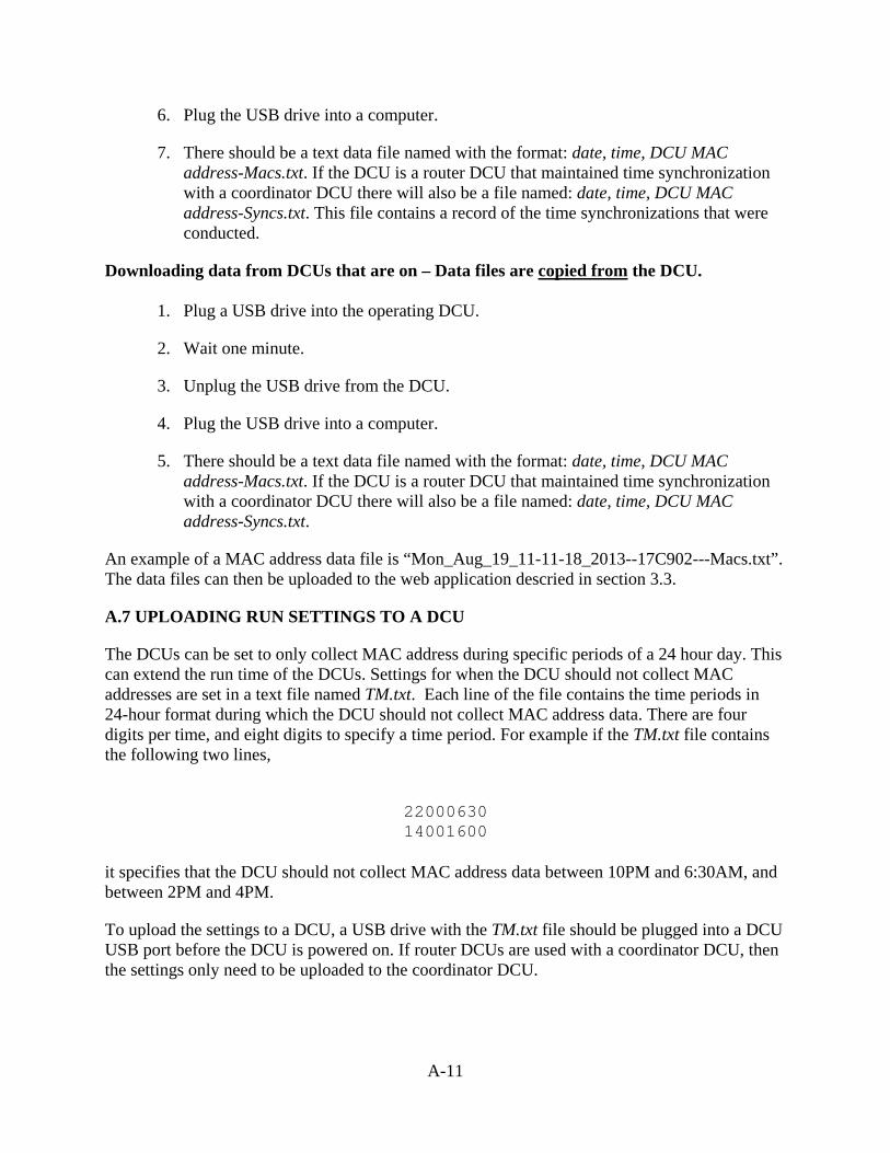
6. Plug the USB drive into a computer.

7. There should be a text data file named with the format: date, time, DCU MAC address-Macs.txt. If the DCU is a router DCU that maintained time synchronization with a coordinator DCU there will also be a file named: date, time, DCU MAC address-Syncs.txt. This file contains a record of the time synchronizations that were conducted.

Downloading data from DCUs that are on – Data files are copied from the DCU.

1. Plug a USB drive into the operating DCU.

2. Wait one minute.

3. Unplug the USB drive from the DCU.

4. Plug the USB drive into a computer.

5. There should be a text data file named with the format: date, time, DCU MAC address-Macs.txt. If the DCU is a router DCU that maintained time synchronization with a coordinator DCU there will also be a file named: date, time, DCU MAC address-Syncs.txt.

An example of a MAC address data file is “Mon_Aug_19_11-11-18_2013--17C902---Macs.txt”. The data files can then be uploaded to the web application descried in section 3.3.

A.7 UPLOADING RUN SETTINGS TO A DCU

The DCUs can be set to only collect MAC address during specific periods of a 24 hour day. This can extend the run time of the DCUs. Settings for when the DCU should not collect MAC addresses are set in a text file named TM.txt. Each line of the file contains the time periods in 24-hour format during which the DCU should not collect MAC address data. There are four digits per time, and eight digits to specify a time period. For example if the TM.txt file contains the following two lines,

22000630 14001600

it specifies that the DCU should not collect MAC address data between 10PM and 6:30AM, and between 2PM and 4PM.

To upload the settings to a DCU, a USB drive with the TM.txt file should be plugged into a DCU USB port before the DCU is powered on. If router DCUs are used with a coordinator DCU, then the settings only need to be uploaded to the coordinator DCU.

A-11

A-1

APPENDIX B – WEB APPLICATION USERS GUIDE

APPENDIX B – WEB APPLICATION USERS GUIDE To process the data collected by the portable data collection system, a web-based (currently hosted on an OSU server) application has been developed. The URL for the application is

http://research.engr.oregonstate.edu/btdataanalysis/logIn.php.

A user will have to register in order to get access to the application, and will need the proper access code in order to register.

The application has been designed with three main data processing and analysis procedures for the following applications:

1. Origin-Destination data collection,

2. Travel time data collection,

3. Intersection performance estimation.

The user of the application will normally execute the following steps after accessing the application.

• Choose the appropriate data processing and analysis procedure for the

application,

• Upload raw data files obtained from the DCUs,

• Enter parameters for the analysis such as the location of the DCUs, the MAC address of the DCUs, the maximum allowed travel time between locations, etc.

• Conduct the analysis, view the results, and copy the results from the application directly into a spreadsheet.

• Close the application.

Each step will be described in more detail.

Selecting a Data Processing and Analysis Procedure. When the application is first visited after signing in, the screen in Figure B.1 will be displayed. The user selects the desired procedure by clicking on one of the three options shown on the left panel in Figure B.1.

B-1

Figure B.1: Initial application screen. Origin-Destination Data Analysis When the Origin-Destination data analysis procedure is selected the screen in Figure B.2 will appear. The screen is asking for the selection of data files (*.txt files) that were downloaded from the DCUs. The files should be accessible on a drive (jump drive or hard drive), and as many files as needed can be selected using the “ctrl” key after clicking on the “browse” button. Do not change the name of the data files since the application only accepts names with a specified format.

After selecting the files, click the “Upload” button. The screen in Figure B.3 will be displayed. It will show the MAC addresses of the DCU that collected the data in each file, and will also display the intervals for which data was collected. Any gap in time that is more than one hour will start a new time interval.

User Input The remainder of the screen shown in Figure B.3 depicts the user input required to process the origin-destination data. These inputs are organized into three steps:

• Step 1

o The number of locations where data was collected.

o The specific time period (within the data collection period) for which origin-destination data is desired. For example if data was collected for five consecutive days this feature can be used to obtain the data for any particular subset of continuous days within the five day period.

B-2

• Step 2

o Assign DCUs to specific locations. The pull down lists will show the MAC addresses of all DCUs providing data files. Locations are referred to by number so the user must map a location number to the actual location. Also note that one or more DCUs may be assigned to a single location.

• Step 3

o The maximum location to location travel times that define trips from an origin to a destination. This must be entered for all location pairs. If a travel time between two locations is greater than the specified maximum travel time, the travel time will be discarded and will not count as a trip. The purpose is to minimize double counting of trips when data is collected over multiple days. For example assume the maximum travel time between all locations is eight hours. Then if a vehicle was detected at location 1 on day 1, and then was detected at location 2 four hours later, and also at location 2 on day 2 and day 3, only one trip will be counted.

Figure B.2: Initial origin-destination analysis screen.

B-3

Figure B.3: User parameter input screen – origin destination data analysis.

Analysis Output After all user inputs have been specified the analysis is started by clicking the Submit button shown on the lower right portion of the screen in Figure B.3. A sample of the analysis output is shown in Figure B.4. To archive the analysis results the user must select and copy information from the screen in Figure B.4 and then paste it into an Excel spreadsheet. Once the analysis output window is closed the results are lost. They can be reproduced by running the analysis again.

B-4

Figure B.4: Analysis output screen – origin destination data analysis. Travel Time Analysis When the Travel Time Analysis procedure is selected the screen in Figure B.5 will appear. The screen is asking for the selection of data files (*.txt files) that were downloaded from the DCUs. The files should be accessible on a drive (jump drive or hard drive), and as many files as needed can be selected using the “ctrl” key after clicking on the “browse” button. Do not change the name of the data files since the application only accepts names with a specified format.

After selecting the files, click the “Upload” button. The screen in Figure B.6 will be displayed. It will show the MAC addresses of the DCU that collected the data in each file, and will also display the intervals for which data was collected. Any gap in time that is more than one hour will start a new time interval.

B-5

Figure B.5: Initial travel time analysis screen.

Figure B.6: User parameter input screen – travel time analysis.

B-6

User Input The remainder of the screen shown in Figure B.6 depicts the user input required for travel time data generation. These inputs are organized into two steps:

• Step 1

o The specific time period (within the data collection period) for which travel time data is desired. For example if data was collected for five consecutive days this feature can be used to obtain the data for any particular subset of continuous days within the five day period.

o The number of road segments for which travel time data is collected must be specified. A road segment is defined by two DCUs – with one DCU at each end of the road segment.

• Step 2 o Assign DCUs to specific road segments. The pull down lists will show the MAC

addresses of all DCUs providing data files. The same DCU may be at the end of one road segment and the beginning of another road segment.

o Specify the maximum road segment travel time. This may be specified as a travel time, or by specifying the road segment length and a minimum average travel speed. If a travel time for a road segment is greater than the specified maximum travel time, the travel time will be discarded. The purpose is to eliminate travel times computed from detections on separate days when data is collected over multiple days. For example assume the maximum travel time for a road segment is 10 minutes. Then if a vehicle was detected at the beginning of the road segment on day 1, and then was detected at the end of the road segment four hours later, the four hour travel time will not be considered (since it is not a road segment travel time).

Analysis Output After all user inputs have been specified the analysis is started by clicking the Submit button shown on the lower right portion of the screen in Figure B.6. A sample of the analysis output is shown in Figure B.7. To archive the analysis results the user must select and copy information from the screen in Figure B.7 and then paste it into an Excel spreadsheet. Once the analysis output window is closed the results are lost. They can be reproduced by running the analysis again.

B-7

Figure B.7: Analysis output screen – travel time data analysis. Intersection Performance Analysis When the Intersection Performance Analysis procedure is selected the screen in Figure B.8 will appear. The screen is asking for the selection of data files (*.txt files) that were downloaded from the DCUs. The files should be accessible on a drive (jump drive or hard drive), and as many files as needed can be selected using the “ctrl” key after clicking on the “browse” button. Do not change the name of the data files since the application only accepts names with a specified format. The screen in Figure B.8 also contains a diagram of how the DCUs monitoring an intersection are to be arranged.

After selecting the files, click the “Upload” button. The screen in Figure B.9 will be displayed. It will show the MAC addresses of the DCU that collected the data in each file, and will also display the intervals for which data was collected. Any gap in time that is more than one hour will start a new time interval.

B-8

Figure B.8: Initial intersection performance analysis screen

Figure B.9: User parameter input screen – intersection performance analysis.

B-9

User Input The remainder of the screen shown in Figure B.9 depicts the user input required to process the origin-destination data. These inputs are organized into three steps:

• Step 1

o The specific time period (within the data collection period) for which origin-destination data is desired. For example if data was collected for five consecutive days this feature can be used to obtain the data for any particular subset of continuous days within the five day period.

o Specify the total number of DCUs being utilized. Indicate the number of DCUs approaching the intersection, and also the number of DCUs that occur after passing through the intersection.

o Indicate the speed limit on the road being monitored. o Specify the distance (feet) between the DCUs. Ideally the DCUs should be

equally spaced along the road, although unequal spacing is acceptable. • Step 2

o Assign DCUs before the intersection to specific locations. The pull down lists will show the MAC addresses of all DCUs providing data files. DCUs farther from the intersection have a larger unit number. For example, if there are four DCUs before the intersection the indicator DCU will unit 4 and the DCU at the intersection will be unit 1. In a similar fashion the DCUs that occur after the intersection start with unit 1 and end with the largest unit number, which is the second indicator DCU.

o Indicate the spacing between the DCUs in feet. • Step 3

o Assign DCUs after the intersection to specific locations. In a similar fashion the DCUs that occur after the intersection start with unit 1 and end with the largest unit number, which is the second indicator DCU.

o Indicate the spacing between the DCUs in feet.

Analysis Output After all user inputs have been specified the analysis is started by clicking the Submit button shown on the lower right portion of the screen in Figure B.9. A sample of the analysis output is shown in Figure B.10. To archive the analysis results the user must select and copy information from the screen in Figure B.10 and then paste it into an Excel spreadsheet. Once the analysis output window is closed the results are lost. They can be reproduced by running the analysis again.

B-10

The results presented are travel time histograms for the travel time between the two indicator DCUs. There are three histograms.

1. All vehicles detected.

2. Through passes.

3. Travel times for vehicles that stopped or almost stopped at the intersection.

Figure B.10: Analysis output screen – intersection performance analysis.

B-11

B-1

APPENDIX C – COMPONENT SPECIFICATIONS

APPENDIX C – COMPONENT SPECIFICATIONS Specifications of the major DCU components are contained in this appendix.

C.1 iMX233-OLinuXino-MINI

FEATURES

• iMX233 ARM926J processor at 454Mhz

• 64 MB RAM

• SD-card connector for booting the Linux image

• TV PAL/NTSC video output

• 3 USB Hi-speed host

• Stereo audio input

• Stereo headphones audio output

• Two buttons

• UEXT connector for connection of different peripherial modules

• 40 pin GPIO for connection of other hardware

• Board is in shape for fit inside Pactec JM42 plastic box

• Power supply input 6-16VDC

C-1

• PCB dimensions: 3.70'' x 2.15'' (94.0mm x 54.6mm)

• Nominal dimensions: 3.70'' x 2.65'' (94.0mm x 67.3mm)

C-2

C.2 Bluetooth Adaptor

C-3

C.3 Zigbee Radio

C-4

C.4 HyperGain HG2408P Antenna

Electrical Specifications Frequency 2400-2500 MHz Gain 8 dBi Horizontal Beam Width 75 degrees Vertical Beam Width 65 degrees Impedance 50 Ohm Max. Input Power 25 Watts VSWR < 1.5:1 avg. Lightning Protection DC Short

Mechanical Specifications

Weight 0.3 lbs. (.13 Kg) Dimensions 4" (102 mm) Dia x 1" (25 mm) Radome Material UV-inhibited Polymer Flame Rating UL 94HB Operating Temperature -40° C to 85° C

(-40° F to 185° F) Mounting Four ¼ in. (6.3 mm) Holes Polarization Horizontal or Vertical Wind Survival >150 MPH (241 KPH) RoHS Compliant Yes

Wind Loading Data

Wind Speed (MPH) Loading 100 3 lb. 125 4 lb.

C-5

Antenna Gain Patterns

C-6

C.5 Specifications of HG2405RD-RSP ZigBee Antenna

Connector Type Reverse Polarity SMA Plug

Diameter 0.5 In.

Finish Matte Black Frequency 2400 to 2500 MHz

Gain 5.5 dBi Impedance 50 Ohm

Length 8.2 In. Polarization Vertical

Temperature, Operating –40°C to 85°C

Weight 0.7 Oz.

Lead Free Status / Rohs Status RoHS Compliant part

C-7