Dr. Corey J. BishopAssistant Professor of Biomedical Engineering

Principal Investigator of the Pharmacoengineering Laboratory:pharmacoengineering.com

Dwight Look College of EngineeringTexas A&M University

Emerging Technologies Building Room 5016College Station, TX 77843

cbishop@tamu.edu

BMOLE 452-689 – TransportChapter 8. Transport in Porous Media

Text Book: Transport Phenomena in Biological SystemsAuthors: Truskey, Yuan, Katz

Focus on what is presented in class and problems…

1How are calculus, alchemy and forging coins related?

Porosity, Tortuosity, and Available Volume Fraction

Chapter 8, Section 2

2

𝑆𝑝𝑒𝑐𝑖𝑓𝑖𝑐 𝑆𝑢𝑟𝑓𝑎𝑐𝑒 = 𝑠 =𝑇𝑜𝑡𝑎𝑙 𝑖𝑛𝑡𝑒𝑟𝑓𝑎𝑐𝑒 𝑎𝑟𝑒𝑎

𝑇𝑜𝑡𝑎𝑙 𝑣𝑜𝑙𝑢𝑚𝑒

𝑃𝑜𝑟𝑜𝑠𝑖𝑡𝑦 = 휀 =𝑉𝑜𝑖𝑑 𝑣𝑜𝑙𝑢𝑚𝑒

𝑇𝑜𝑡𝑎𝑙 𝑣𝑜𝑙𝑢𝑚𝑒

Units = 1

𝑙𝑒𝑛𝑔𝑡ℎ

휀 is dimensionless

Void volume: total volume of void space in a porous medium

Interface: border between solid and void spaces

If total volume based on interstitial space: 휀 is larger than 0.9If cells and vessels need to be considered: 휀 varies between 0.06 and 0.30Note: In some tumors, 휀 is as high as 0.6

3

Porosity (휀)• Porosity: a measure of the average void volume fraction in a specific

region of porous medium• Does not provide information on how pores are connected or number of

pores available for water and solute transport

휀 = 휀𝑖 + 휀𝑝 + 휀𝑛

Note: isolated pores are not accessible to external solvents and solutes:They can sometimes be considered part of the solid phase.In this case, void volume is the total volume of penetrable pores

4

Tortuosity (T)• Path length between A and B in a porous medium is the distance

between the points through connected pores• Lmin is the shorted path length

• L is the straight-line distance between A and B

𝑇 = (𝐿𝑚𝑖𝑛

𝐿)2

T is always greater than or equal to unity

5

Available Volume Fraction (𝐾𝐴𝑉)• Not all penetrable pores are accessible to solutes: Dependent on

molecular properties of the solutes• Pore smaller than solute molecule or is surrounded by too small pores

• Available Volume: portion of accessible volume that can be occupied by the solute

𝐾𝐴𝑉 =𝐴𝑣𝑎𝑖𝑙𝑎𝑏𝑙𝑒 𝑣𝑜𝑙𝑢𝑚𝑒

𝑇𝑜𝑡𝑎𝑙 𝑣𝑜𝑙𝑢𝑚𝑒

6

𝐾𝐴𝑉 is molecule dependent and always smaller than porosity.

This can be caused by 3 scenarios:1)Centers of the solute molecules cannot reach the solid surface in the void space

Difference between total void volume and the available volume can be estimated as the product of the area of the surface and distance (∆) between solute and surface

2)Some of the void space is smaller than the solute molecules3)Inaccessibility of large penetrable pores surrounded by pores smaller than the solutes

Generally, 𝐾𝐴𝑉 decreases with size of solutes

7

• Partition Coefficient (Φ): ratio of available volume to void volume• Measure of solute partitioning at equilibrium between external solutions and

void space in porous media

• Radius of Gyration (Rg): size of flexible molecules

Φ =𝐾𝐴𝑉휀

𝑅𝑔2 =

1

𝑁

𝑖

𝑟𝑖𝑐2 =

1

2𝑁2

𝑖

𝑗

𝑟𝑖𝑗2

𝑟𝑖𝑐 is the average distance between segment i and the center of mass of the polymer chain𝑟𝑖𝑗 is the average distance between segments i and j in the polymer chain

N is the total number of segments in the polymer chain

8

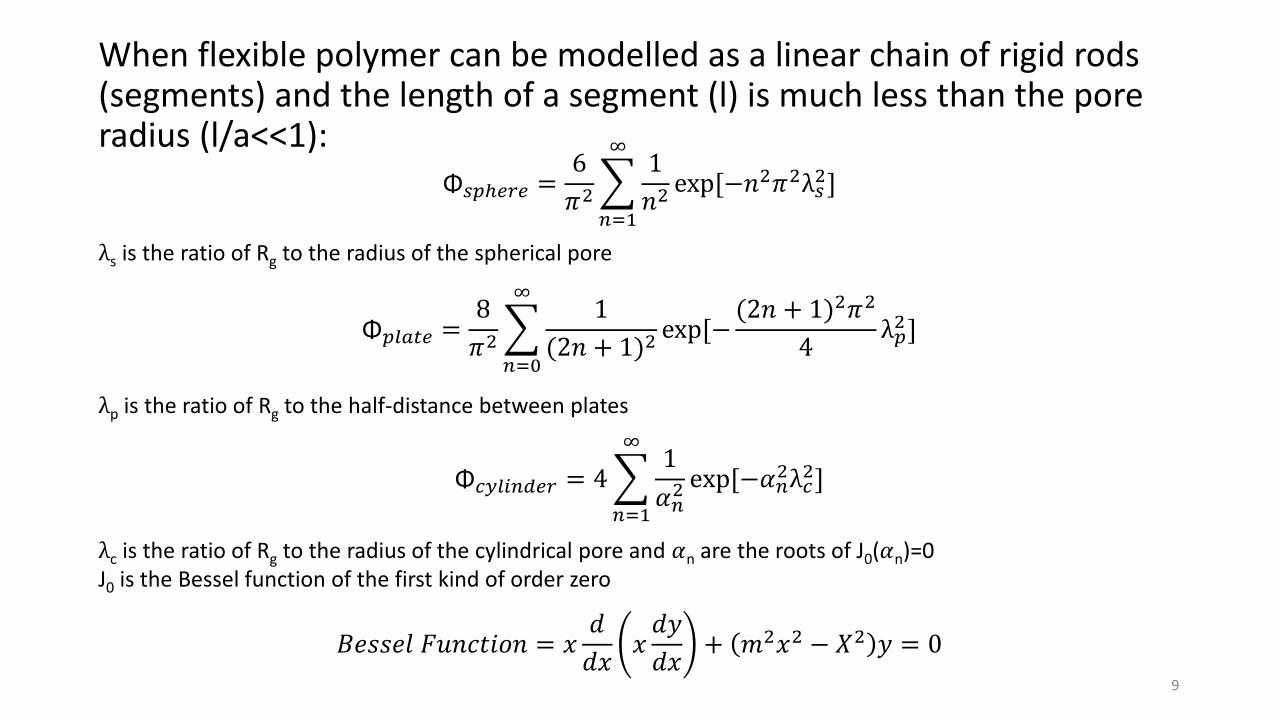
When flexible polymer can be modelled as a linear chain of rigid rods (segments) and the length of a segment (l) is much less than the pore radius (l/a<<1):

Φ𝑠𝑝ℎ𝑒𝑟𝑒 =6

𝜋2

𝑛=1

∞1

𝑛2exp[−𝑛2𝜋2λ𝑠

2]

Φ𝑝𝑙𝑎𝑡𝑒 =8

𝜋2

𝑛=0

∞1

(2𝑛 + 1)2exp[−

(2𝑛 + 1)2𝜋2

4λ𝑝2]

Φ𝑐𝑦𝑙𝑖𝑛𝑑𝑒𝑟 = 4

𝑛=1

∞1

𝛼𝑛2 exp[−𝛼𝑛

2λ𝑐2]

λs is the ratio of Rg to the radius of the spherical pore

λp is the ratio of Rg to the half-distance between plates

λc is the ratio of Rg to the radius of the cylindrical pore and 𝛼n are the roots of J0(𝛼n)=0J0 is the Bessel function of the first kind of order zero

𝐵𝑒𝑠𝑠𝑒𝑙 𝐹𝑢𝑛𝑐𝑡𝑖𝑜𝑛 = 𝑥𝑑

𝑑𝑥𝑥𝑑𝑦

𝑑𝑥+ 𝑚2𝑥2 − 𝑋2 𝑦 = 0

9

Exclusion Volume• Some porous media are fiber matrices: space inside and near surface

of fibers not available to solutes

• Exclusion Volume: size of the space

𝐸𝑥𝑐𝑙𝑢𝑠𝑖𝑜𝑛 𝑣𝑜𝑙𝑢𝑚𝑒 = 𝜋(𝑟𝑓 + 𝑟𝑠)2𝐿

rf and rs are the radii of the fiber and soluteL is the length of the fiber

If minimum distance between fibers is larger than 2(𝑟𝑓 + 𝑟𝑠), such as when fiber density

is very low or when fibers are parallel:

𝐸𝑥𝑐𝑙𝑢𝑠𝑖𝑜𝑛 𝑣𝑜𝑙𝑢𝑚𝑒 𝑓𝑟𝑎𝑐𝑡𝑖𝑜𝑛 =𝜋(𝑟𝑓 + 𝑟𝑠)

2𝐿𝑁

𝑉= 𝜃(

𝑟𝑠𝑟𝑓+ 1)2

θ is the volume fraction of fibers

𝐾𝐴𝑉 = 1 − 𝑒𝑥𝑐𝑙𝑢𝑠𝑖𝑜𝑛 𝑣𝑜𝑙𝑢𝑚𝑒 𝑓𝑟𝑎𝑐𝑡𝑖𝑜𝑛 = 1 − 𝜃𝑟𝑠𝑟𝑓+ 1

2

10

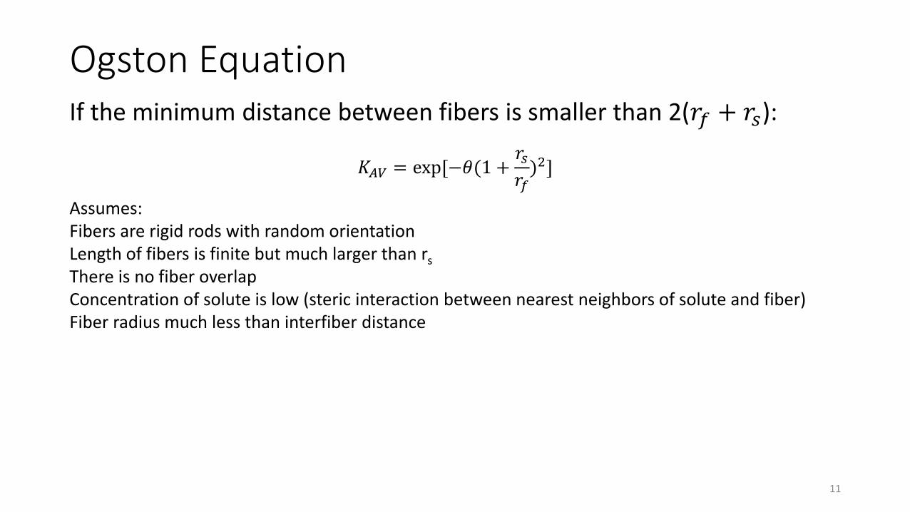
Ogston EquationIf the minimum distance between fibers is smaller than 2(𝑟𝑓 + 𝑟𝑠):

𝐾𝐴𝑉 = exp[−𝜃(1 +𝑟𝑠𝑟𝑓)2]

Assumes:Fibers are rigid rods with random orientationLength of fibers is finite but much larger than rs

There is no fiber overlapConcentration of solute is low (steric interaction between nearest neighbors of solute and fiber)Fiber radius much less than interfiber distance

11

When 𝜃(1 +𝑟𝑠

𝑟𝑓)2 is much less than unity, Ogston Equation reduces to previous equation.

Porosity can be derived from the Ogston Equation by letting rs=0

휀 = exp[−𝜃]

When θ is much less than unity:

휀 = 1 − 𝜃

Partition coefficient of solutes in liquid phase of fiber-matrix material:

Φ =

exp[−𝜃(1 + (𝑟𝑠𝑟𝑓))2]

1 − 𝜃

12

8.3.2: Brinkman Equation

8.3.3: Squeeze Flow

Review: Darcy’s Law

o Describes fluid flow in porous media

o Invalid for Non-Newtonian Fluids

o We talked about 𝛿, 𝑙, 𝑎𝑛𝑑 𝐿o L is the distance over which macroscopic changes of physical quantities have to be considered

o 𝑉 = −𝐾𝛻𝑝o K is the hydraulic conductivity (a constant)o 𝛻𝑝 is the gradient of hydrostatic pressure

o 𝛻𝑉 = −𝛻 𝐾𝛻𝑝 = ϕB − ϕLo ϕB is volumetric flow in sourceo ϕL is volumetric flow in sink o Generally ϕB = ϕL = 0

o Darcy’s Law Neglects Friction within the fluid

Brinkman Equation

o𝑘 = 𝐾𝜇o k is the specific hydraulic permeability (usually units of nm2)oDarcy’s law is used when k is low: when k is much smaller than the square of LoWhen k is not low: Brinkman Equation

o𝐵𝑟𝑖𝑛𝑘𝑚𝑎𝑛 𝐸𝑞𝑢𝑎𝑡𝑖𝑜𝑛:o𝜇𝛻2𝑉 −

1

𝐾𝑉 − 𝛻𝑝=0

oDarcy’s Law is a special case of this equation when the first term = 0 (𝑉 =− 𝐾𝛻𝑝)

Example 8.7!! (The math is annoying and long and I’m sorry) (It’s not my fault) (Don’t hate me)

Ex 8.7

Squeeeze Flow

o Squeeze flow is the fluid flow caused by the relative movement of solid boundaries towards each other

o Tissue deformation causes change in volume fraction of the interstitial spaceo Leads to fluid flow

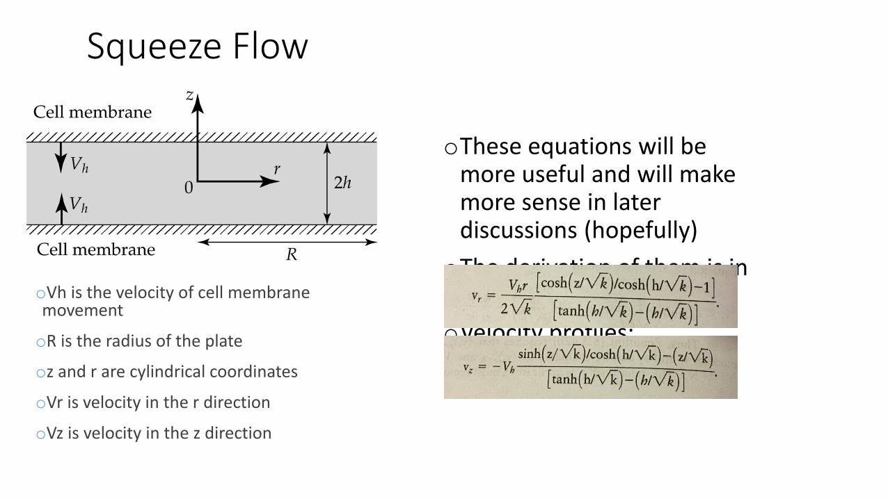
Squeeze Flow

oThese equations will be more useful and will make more sense in later discussions (hopefully)

oThe derivation of them is in 8.3.3

oVelocity profiles:

oVh is the velocity of cell membrane movement

oR is the radius of the plate

oz and r are cylindrical coordinates

oVr is velocity in the r direction

oVz is velocity in the z direction

Darcy’s Law

Darcy’s Law

• Flow rate is proportional to pressure gradient

• Valid in many porous media

• NOT valid for:• Non-Newtonian fluids

• Newtonian liquids at high velocities

• Gasses at very low and high velocities

Darcy’s Law

Describing fluid flow in porous media

• Two Ways:• Numerically solve governing equations for fluid flow in individual pores if

structure is known

• Assume porous medium is a uniform material (Continuum Approach)

Three Length Scales

1. 𝛿 = average size of pores

2. L = distance which macroscopic changes of physical quantities must be considered (ie. Fluid velocity and pressure)

3. 𝑙 = a small volume with dimension 𝑙

Continuum Approach Requires:

• 𝛿 << 𝑙0 << L

Darcy’s Law

• 𝑙0 = Representative Elementary Volume (REV• 𝑙0 << L

• Total volume of REV can give the averaging over a volume value

• vf = fluid velocity, velocity of each fluid particle AVERAGED over volume of the fluid phase

• v = velocity of each fluid particle averaged over REV

• V = 휀Vf

Darcy’s Law

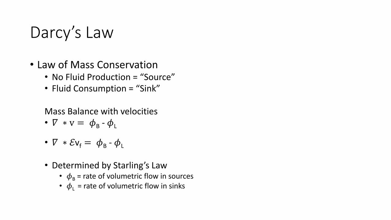
• Law of Mass Conservation• No Fluid Production = “Source”• Fluid Consumption = “Sink”

Mass Balance with velocities• 𝛻 ∗ v = 𝜙B - 𝜙L

• 𝛻 ∗ ℰvf = 𝜙B - 𝜙L

• Determined by Starling’s Law• 𝜙B = rate of volumetric flow in sources• 𝜙L = rate of volumetric flow in sinks

Darcy’s Law

• Momentum Balance in Porous Media• v = -K 𝛻p

• 𝛻p = gradient of hydrostatic pressure

• K = hydraulic conductivity constant

• p = average quantity within the fluid phase in the REV

Darcy’s Law

• Substituting the Equations to form:• 𝛻 ∗ (−K 𝛻p) = 𝜙B - 𝜙L

• Steady State:• 𝛻2 * p = 0

8.4 Solute Transport in Porous Media

8.4.1-8.4.2

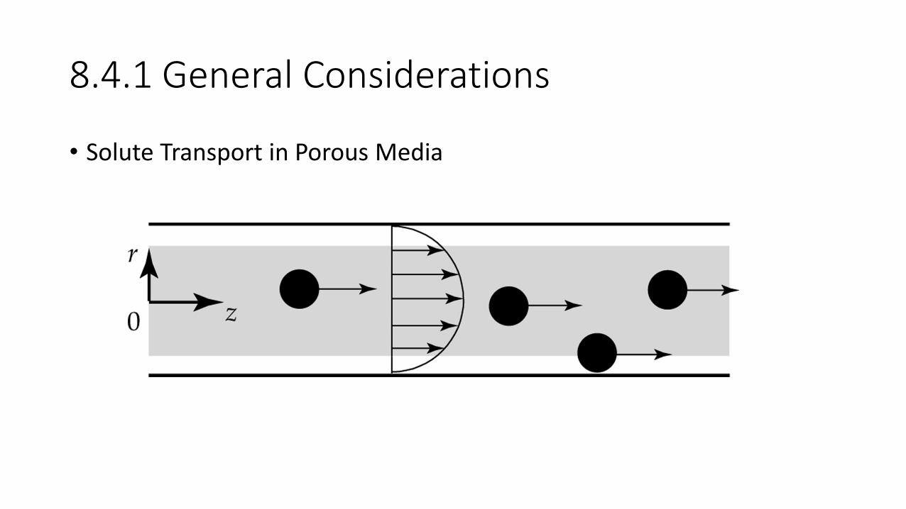
8.4.1 General Considerations

• Solute Transport in Porous Media

8.4.1 General Considerations

1)𝐷𝑒𝑓𝑓 2) Solute velocity

3) Dispersion4) Boundary Conditions

• There are 4 general problems using the continuum approach(Darcy’s Law) for analyzing transport of solutes through porous media

1) 𝐷𝑒𝑓𝑓

• Diffusion of solutes is characterized by the effective diffusion coefficient: 𝐷𝑒𝑓𝑓

• 𝐷𝑒𝑓𝑓 in porous media < 𝐷𝑒𝑓𝑓 in solutions Why?...

1) 𝐷𝑒𝑓𝑓 cont.

• Factor effecting Diffusion in Porous Media:• Connectedness of Pores

1 100Layer #

𝐷𝑒𝑓𝑓Layer 100

Layer 1

As we near layer 100, available space for diffusion and 𝐷𝑒𝑓𝑓 decrease exponentially

2) Solute Velocity

• Convective velocities ≠ Solvent velocities

• Solutes are hindered by porous structures• Ex: filtering coffee grounds

𝑓 =𝑣𝑠

𝑣𝑓=

𝑠𝑜𝑙𝑢𝑡𝑒 𝑣𝑒𝑙𝑜𝑐𝑖𝑡𝑦

𝑠𝑜𝑙𝑣𝑒𝑛𝑡 𝑣𝑒𝑙𝑜𝑐𝑖𝑡𝑦

𝑓 is retardation coefficient

2) Solvent Velocity cont.

• 𝜎 = 1 − 𝑓 : reflection coefficient • Characterizes the hindrance of convective

transport across a membrane

• 𝑓 is dependent on:• Fluid velocity • Solute size• Pore Structure

• Flux of Convective transport across tissue:

𝑁𝑠 = 𝑣𝑠𝐶 = 𝑓𝑣𝑓𝐶

Where 𝑣𝑠is solute velocity and 𝐶 is local concentration of solutes

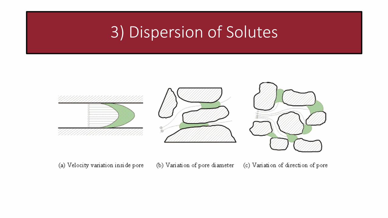
3) Dispersion of Solutes

4) Boundary Conditions

• Concentrations of solutes can be discontinuous at interfases between solutions and porous media• Thus, for two regions, 1 and 2

𝑁1 = 𝑁2

and

𝐶1

𝐾𝐴𝐴1=

𝐶2

𝐾𝐴𝐴2

N = flux

𝐾𝐴𝐴 = area fraction available at inerfase for solute transport

When all 4 are considered…

Governing Equation for Transport of neutral molecule through porous media:

𝜕𝐶

𝜕𝑡+ 𝛻 𝑓𝑣𝑓𝐶 = 𝐷𝑒𝑓𝑓𝛻

2𝐶 + 𝜙𝐵 − 𝜙𝐿 + 𝑄

Flux of Convective Transport

Isotropic, uniform and dispersion coefficient is

negligible

Solute vel. Reaction

If we do consider dispersion coefficient: Deff = Deff + Disp. Coeff.

Governing Equation cont.

𝜕𝐶

𝜕𝑡+ 𝛻 𝑓𝑣𝑓𝐶 = 𝐷𝑒𝑓𝑓𝛻

2𝐶 + 𝜙𝐵 − 𝜙𝐿 + 𝑄

𝐶, 𝜙𝐵 , 𝜙𝐿 , 𝑄:𝑎𝑣𝑔. 𝑞𝑢𝑎𝑛𝑡𝑖𝑡𝑦

𝑢𝑛𝑖𝑡 𝑡𝑖𝑠𝑠𝑢𝑒 𝑣𝑜𝑙𝑢𝑚𝑒

𝑓, 𝑣𝑓 , 𝐷𝑒𝑓𝑓:𝑎𝑣𝑔. 𝑞𝑢𝑎𝑛𝑡𝑖𝑡𝑦

𝑢𝑛𝑖𝑡 𝑣𝑜𝑙𝑢𝑚𝑒 𝑜𝑓 𝑓𝑙𝑢𝑖𝑑 𝑝ℎ𝑎𝑠𝑒

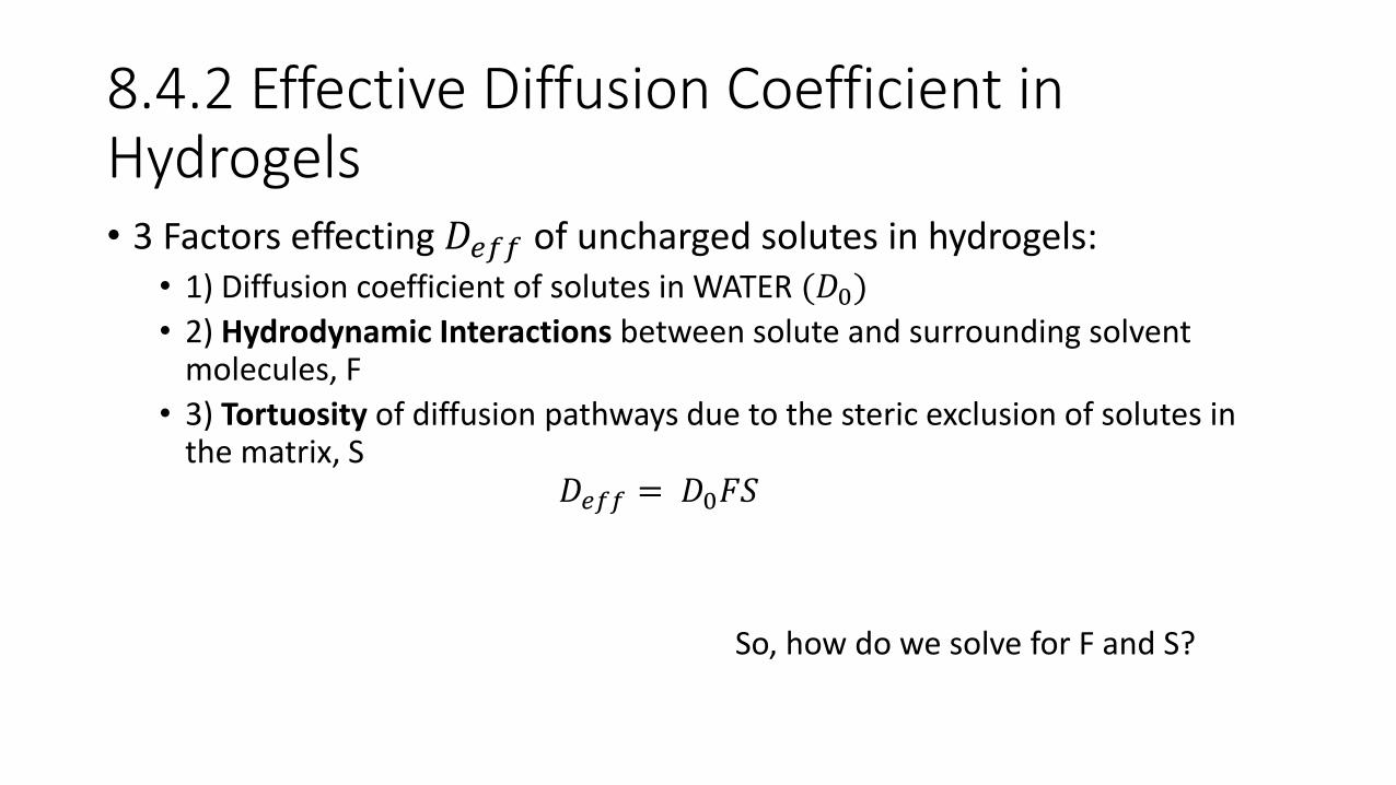
8.4.2 Effective Diffusion Coefficient in Hydrogels• 3 Factors effecting 𝐷𝑒𝑓𝑓 of uncharged solutes in hydrogels:

• 1) Diffusion coefficient of solutes in WATER (𝐷0)

• 2) Hydrodynamic Interactions between solute and surrounding solvent molecules, F

• 3) Tortuosity of diffusion pathways due to the steric exclusion of solutes in the matrix, S

𝐷𝑒𝑓𝑓 = 𝐷0𝐹𝑆

So, how do we solve for F and S?

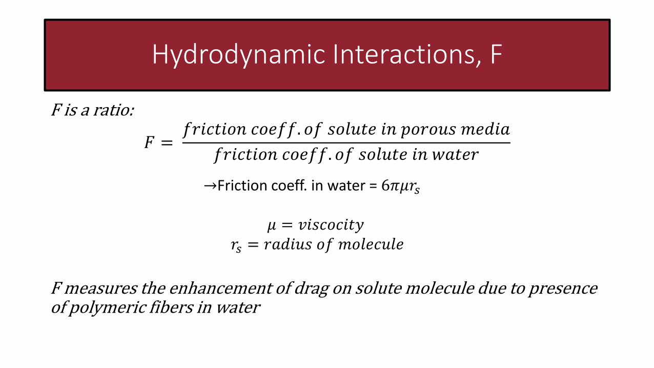
Hydrodynamic Interactions, F

F is a ratio:

𝐹 =𝑓𝑟𝑖𝑐𝑡𝑖𝑜𝑛 𝑐𝑜𝑒𝑓𝑓. 𝑜𝑓 𝑠𝑜𝑙𝑢𝑡𝑒 𝑖𝑛 𝑝𝑜𝑟𝑜𝑢𝑠 𝑚𝑒𝑑𝑖𝑎

𝑓𝑟𝑖𝑐𝑡𝑖𝑜𝑛 𝑐𝑜𝑒𝑓𝑓. 𝑜𝑓 𝑠𝑜𝑙𝑢𝑡𝑒 𝑖𝑛 𝑤𝑎𝑡𝑒𝑟

F measures the enhancement of drag on solute molecule due to presence of polymeric fibers in water

→Friction coeff. in water = 6𝜋𝜇𝑟𝑠

𝜇 = 𝑣𝑖𝑠𝑐𝑜𝑐𝑖𝑡𝑦𝑟𝑠 = 𝑟𝑎𝑑𝑖𝑢𝑠 𝑜𝑓 𝑚𝑜𝑙𝑒𝑐𝑢𝑙𝑒

Hydrodynamic Interactions, F cont.

1) Effective-medium or

Brinkman-medium

2) 3-D space with cylindrical fibers

model

Two approaches to determining F:

1) Effective-Medium or Brinkman-Medium

• Assumptions: • Hydrogel is a uniform medium

• Spherical solute molecule

• Constant velocity

• Movement governed by Brinkman Equation

𝐹 = 1 +𝑟𝑠

𝑘+1

9

𝑟𝑠

𝑘

2 −1

where 𝜙𝐵 = 𝜙𝐿 = 0

2) 3-D space with cylindrical fibers model

• Assumptions: • Hydrogel is modeled as 3-D

spaces filled with water and randomly placed cylindrical fibers

• Movement of spherical particles is determined by Stokes-Einstein Equation

𝐹 𝛼, 𝜃 = exp(−𝑎1𝜃𝑎2) pg. 426

→done after normalization of 6𝜋𝜇𝑟𝑠

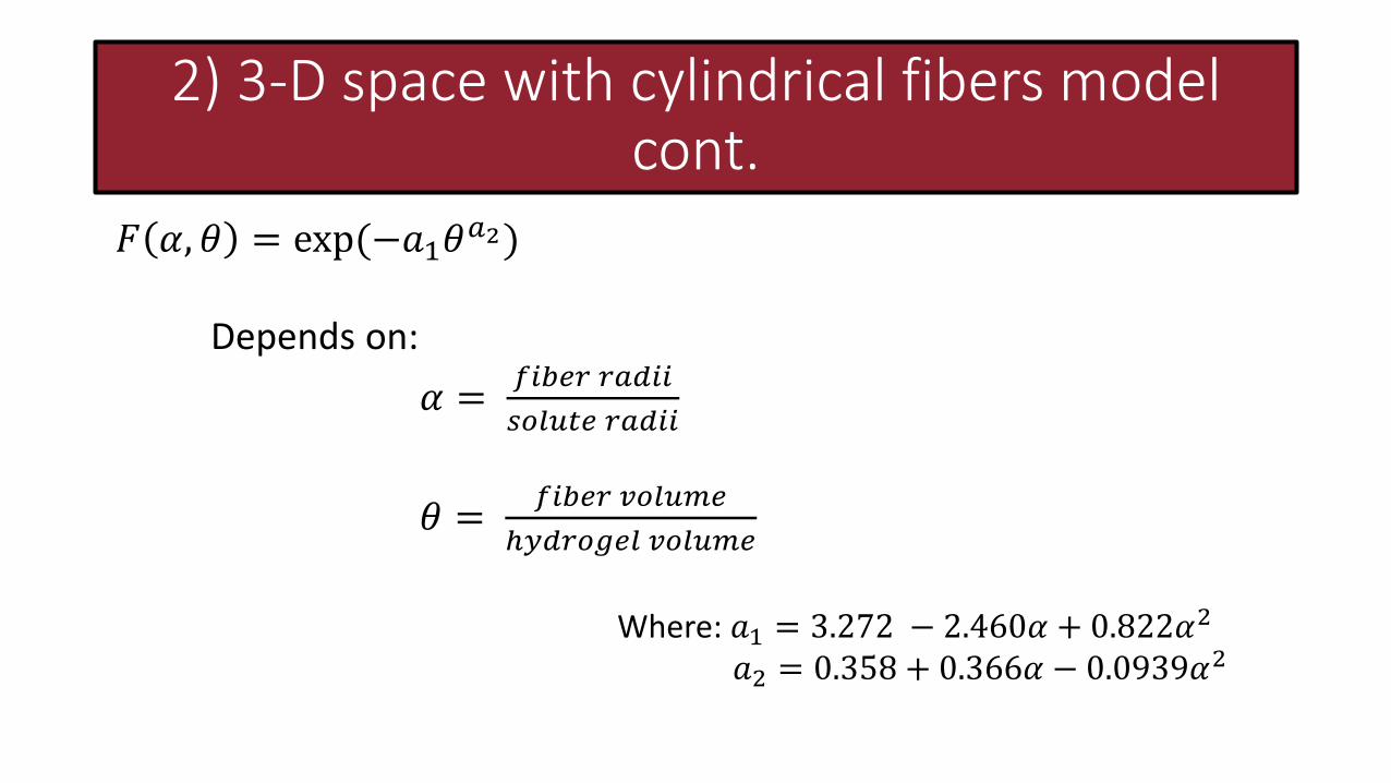
2) 3-D space with cylindrical fibers model cont.

𝐹 𝛼, 𝜃 = exp(−𝑎1𝜃𝑎2)

Depends on:

𝛼 =𝑓𝑖𝑏𝑒𝑟 𝑟𝑎𝑑𝑖𝑖

𝑠𝑜𝑙𝑢𝑡𝑒 𝑟𝑎𝑑𝑖𝑖

𝜃 =𝑓𝑖𝑏𝑒𝑟 𝑣𝑜𝑙𝑢𝑚𝑒

ℎ𝑦𝑑𝑟𝑜𝑔𝑒𝑙 𝑣𝑜𝑙𝑢𝑚𝑒

Where: 𝑎1 = 3.272 − 2.460𝛼 + 0.822𝛼2

𝑎2 = 0.358 + 0.366𝛼 − 0.0939𝛼2

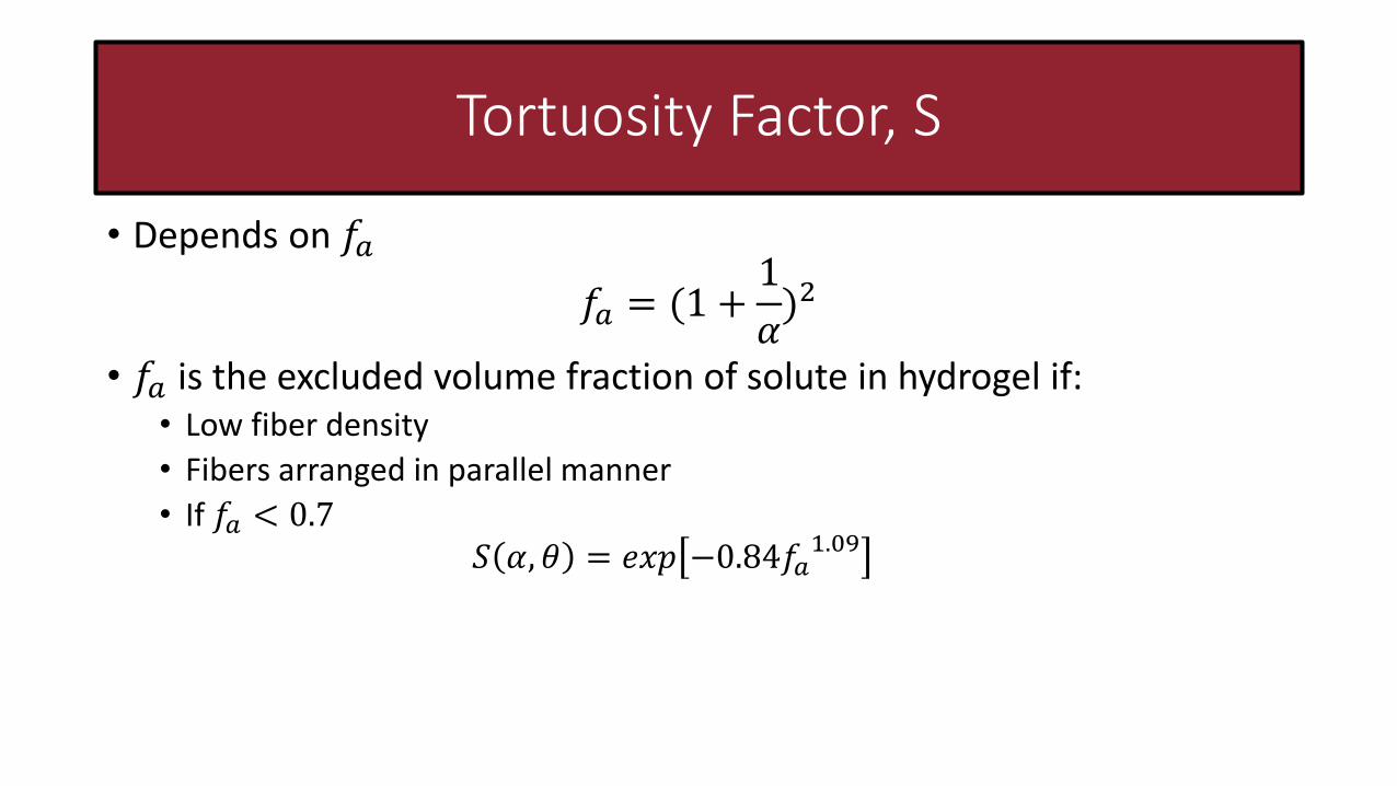
Tortuosity Factor, S

• Depends on 𝑓𝑎

𝑓𝑎 = (1 +1

𝛼)2

• 𝑓𝑎 is the excluded volume fraction of solute in hydrogel if: • Low fiber density

• Fibers arranged in parallel manner

• If 𝑓𝑎 < 0.7𝑆 𝛼, 𝜃 = 𝑒𝑥𝑝 −0.84𝑓𝑎

1.09

Effective Diffusion Coefficient: In Liquid-Filled Pore and Biological

TissueChapter 8: Section 4.3-4.4

45

Effective Diffusion Coefficient in a Liquid-Filled Pore• Depends on diffusion coefficient D0 of solutes in water, hydrodynamic

interactions between solute and solvent molecules, and steric exclusion of solutes near the walls of pores

• Assume entrance effect is negligible:

𝑣𝑧 = 2𝑣𝑚(1 −𝑟

𝑅)2

vz is the axial fluid velocityvm is the mean velocity in the porer is the radial coordinate R is the radii of the cylinder

46

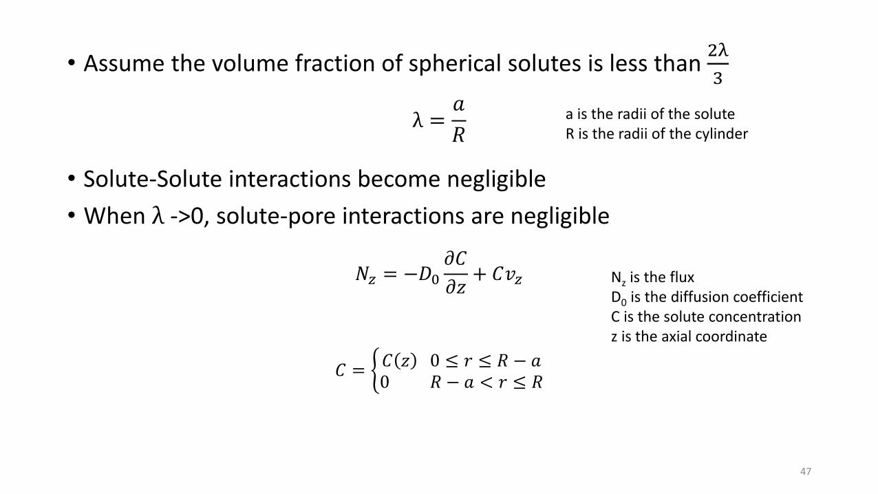
• Assume the volume fraction of spherical solutes is less than 2λ

3

• Solute-Solute interactions become negligible

• When λ ->0, solute-pore interactions are negligible

λ =𝑎

𝑅a is the radii of the soluteR is the radii of the cylinder

𝑁𝑧 = −𝐷0𝜕𝐶

𝜕𝑧+ 𝐶𝑣𝑧 Nz is the flux

D0 is the diffusion coefficientC is the solute concentration z is the axial coordinate

𝐶 = ቊ𝐶 𝑧 0 ≤ 𝑟 ≤ 𝑅 − 𝑎0 𝑅 − 𝑎 < 𝑟 ≤ 𝑅

47

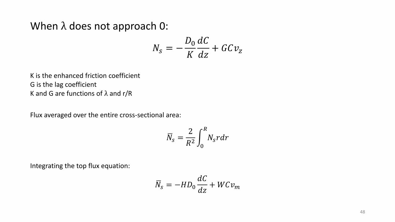
When λ does not approach 0:

𝑁𝑠 = −𝐷0𝐾

𝑑𝐶

𝑑𝑧+ 𝐺𝐶𝑣𝑧

K is the enhanced friction coefficientG is the lag coefficientK and G are functions of λ and r/R

Flux averaged over the entire cross-sectional area:

ഥ𝑁𝑠 =2

𝑅2න0

𝑅

𝑁𝑠𝑟𝑑𝑟

Integrating the top flux equation:

ഥ𝑁𝑠 = −𝐻𝐷0𝑑𝐶

𝑑𝑧+𝑊𝐶𝑣𝑚

48

H and W are called hydrodynamic resistance coefficients

𝐻 =2

𝑅2න0

𝑅−𝑎 1

𝐾𝑟𝑑𝑟

𝑊 =4

𝑅2න0

𝑅−𝑎

𝐺 1 −𝑟

𝑅

2

𝑟𝑑𝑟

49

𝐷𝑒𝑓𝑓 = 𝐻𝐷0

Centerline approximation: assume all spheres are distributed on the centerline position in the poreFor λ < 0.4:

𝐾−1 λ, 0 = 1 − 2.1044λ + 2.089λ3 − 0.948λ5

𝐺 λ, 0 = 1 −2

3λ2 − 0.163λ3

50

𝐻 λ = Φ 1 − 2.1044λ + 2.089λ3 − 0.948λ5

𝑊 λ = Φ 2 −Φ 1 −2

3λ2 − 0.163λ3

Φ = 1 − λ 2Partition coefficient of solute in the pore:

For λ > 0.4:

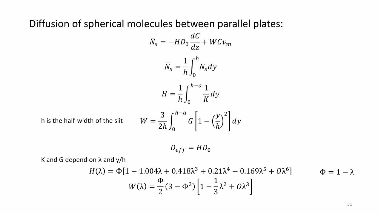
Diffusion of spherical molecules between parallel plates:

51

ഥ𝑁𝑠 = −𝐻𝐷0𝑑𝐶

𝑑𝑧+𝑊𝐶𝑣𝑚

ഥ𝑁𝑠 =1

ℎන0

ℎ

𝑁𝑠𝑑𝑦

𝐻 =1

ℎන0

ℎ−𝑎 1

𝐾𝑑𝑦

𝑊 =3

2ℎන0

ℎ−𝑎

𝐺 1 −𝑦

ℎ

2

𝑑𝑦h is the half-width of the slit

𝐷𝑒𝑓𝑓 = 𝐻𝐷0

K and G depend on λ and y/h

𝐻 λ = Φ 1 − 1.004λ + 0.418λ3 + 0.21λ4 − 0.169λ5 + 𝑂λ6

𝑊 λ =Φ

23 − Φ2 1 −

1

3λ2 + 𝑂λ3

Φ = 1 − λ

Effective Diffusion Coefficient in Biological Tissues

𝐷𝑒𝑓𝑓 = 𝑏1 𝑀𝑟−𝑏2

Mr is the molecular weight of the solutesb1 and b2 are functions of charge and shape of solutes, and structures of tissues

The effects of tissue structures on Deff increases with the size of solutes

52

Fluid Transport in Poroelastic Materials

Section 8.5

By: Hannah Humbert

53

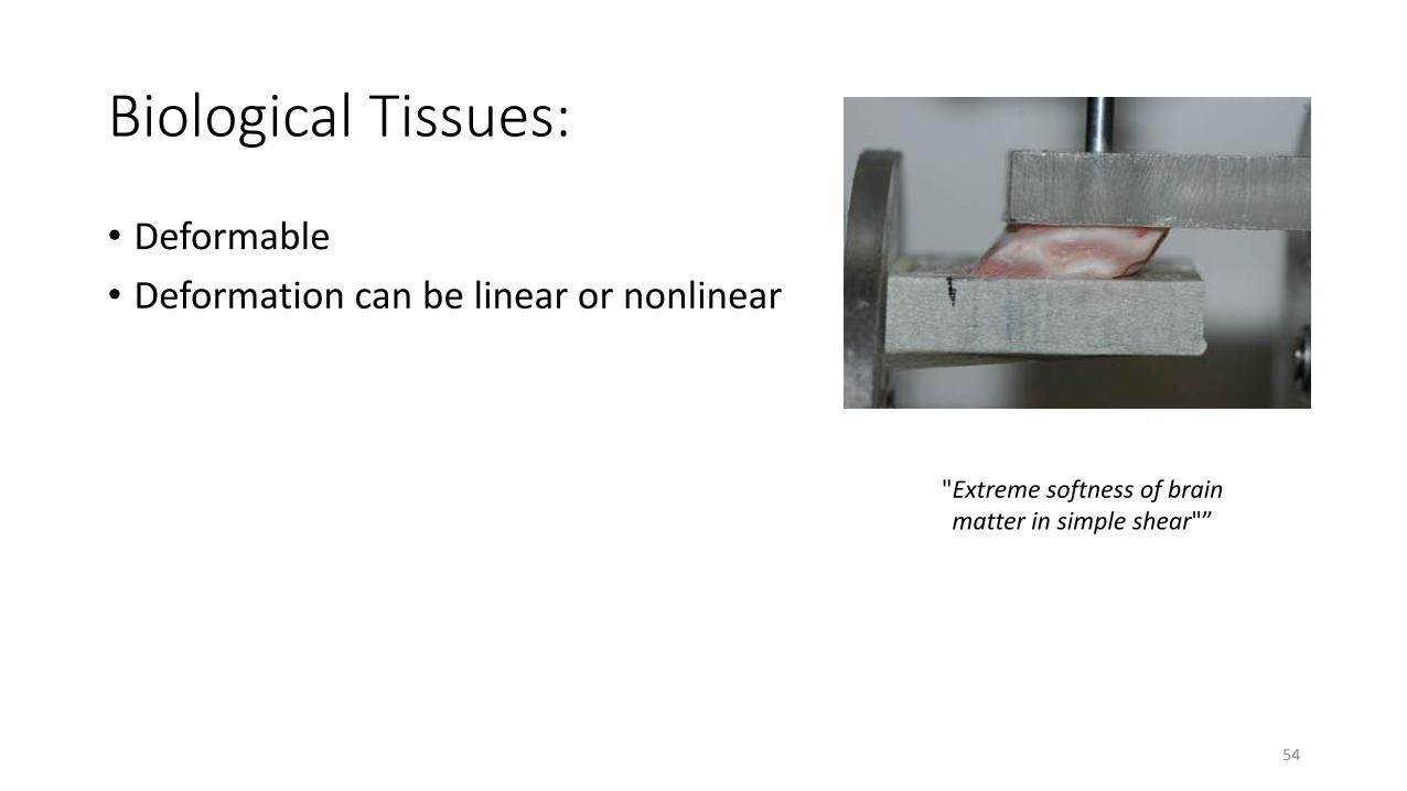
Biological Tissues:

• Deformable

• Deformation can be linear or nonlinear

54

"Extreme softness of brain matter in simple shear"”

Poroelastic Response

55

𝜎𝑥𝑥𝜎𝑥𝑥

𝜎𝑦𝑦

𝜎𝑦𝑦

𝑥

𝑦

𝜎𝑥𝑦

Total Stress = Effective Stress + Pore Pressure

𝝈 = 𝝉 + 𝑝𝑰

Pore Fluid Pressure, 𝑝

Porosity, ε

56

𝝈 =

𝜏𝑥𝑥 𝜏𝑥𝑦 𝜏𝑥𝑧𝜏𝑦𝑥 𝜏𝑦𝑦 𝜏𝑦𝑧𝜏𝑧𝑥 𝜏𝑧𝑦 𝜏𝑧𝑧

+

𝑝 0 00 𝑝 00 0 𝑝

= 2𝜇𝐺𝑬 + 𝜇λ𝑒𝑰 + 𝑝𝑰

𝑰 =1 0 00 1 00 0 1

Must be describing stresses that are NOT pore pressure related

If,

then,

Understanding the linear function of Stress

Understanding the linear Function of Stress

57

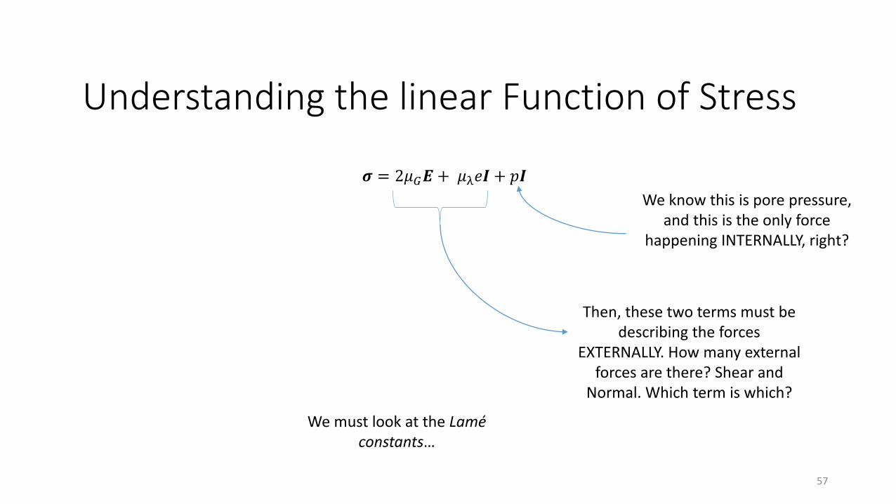
𝝈 = 2𝜇𝐺𝑬 + 𝜇λ𝑒𝑰 + 𝑝𝑰

We know this is pore pressure, and this is the only force

happening INTERNALLY, right?

Then, these two terms must be describing the forces

EXTERNALLY. How many external forces are there? Shear and

Normal. Which term is which?

We must look at the Laméconstants…

LamÉ Constants

• Named after French Mathematician, Gabriel Lamé• Two constants which relate stress to strain in isotropic, elastic

material• Depend on the material and its temperature

58

𝝁𝝀 : first parameter (related to bulk modulus)𝝁𝑮 : second parameter (related to shear modulus)

𝜇𝜆 = 𝐾 − ൗ2 3 𝜇𝐺

𝜇𝐺 =𝜏

𝛾=

∆𝐹𝐴∆𝐿𝐿

Understanding the linear Function of Stress

59

𝝈 = 2𝜇𝐺𝑬 + 𝜇λ𝑒𝑰 + 𝑝𝑰

Describes INTERNAL FORCES

Describes EXTERNAL BULK

FORCES

Describes EXTERNAL SHEAR

FORCES

Now we need to understand E and e…

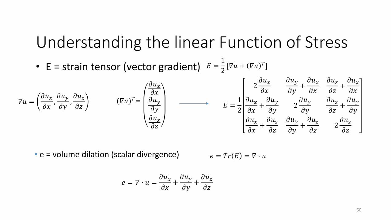
• E = strain tensor (vector gradient)

60

Understanding the linear Function of Stress𝐸 =

1

2[𝛻𝑢 + 𝛻𝑢 𝑇]

𝐸 =1

2

2𝜕𝑢𝑥𝜕𝑥

𝜕𝑢𝑦

𝜕𝑦+𝜕𝑢𝑥𝜕𝑥

𝜕𝑢𝑧𝜕𝑧

+𝜕𝑢𝑥𝜕𝑥

𝜕𝑢𝑥𝜕𝑥

+𝜕𝑢𝑦

𝜕𝑦2𝜕𝑢𝑦

𝜕𝑦

𝜕𝑢𝑧𝜕𝑧

+𝜕𝑢𝑦

𝜕𝑦

𝜕𝑢𝑥𝜕𝑥

+𝜕𝑢𝑧𝜕𝑧

𝜕𝑢𝑦

𝜕𝑦+𝜕𝑢𝑧𝜕𝑧

2𝜕𝑢𝑧𝜕𝑧

𝛻𝑢 =𝜕𝑢𝑥𝜕𝑥

,𝜕𝑢𝑦

𝜕𝑦,𝜕𝑢𝑧𝜕𝑧

(𝛻𝑢)𝑇=

𝜕𝑢𝑥𝜕𝑥𝜕𝑢𝑦𝜕𝑦𝜕𝑢𝑧𝜕𝑧

• e = volume dilation (scalar divergence) 𝑒 = 𝑇𝑟 𝐸 = 𝛻 ∙ 𝑢

𝑒 = 𝛻 ∙ 𝑢 =𝜕𝑢𝑥𝜕𝑥

+𝜕𝑢𝑦

𝜕𝑦+𝜕𝑢𝑧𝜕𝑧

61

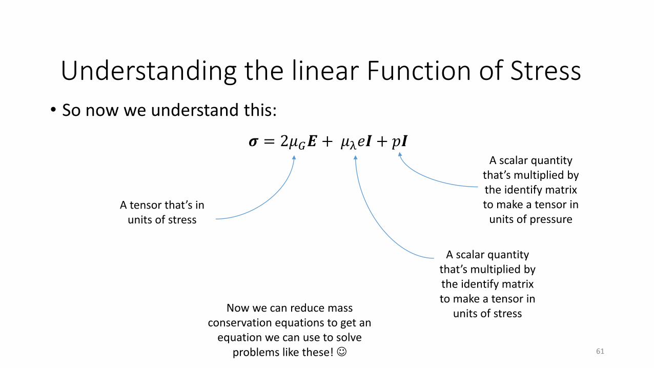
Understanding the linear Function of Stress• So now we understand this:

𝝈 = 2𝜇𝐺𝑬 + 𝜇λ𝑒𝑰 + 𝑝𝑰A scalar quantity

that’s multiplied by the identify matrix to make a tensor in

units of pressure

A scalar quantity that’s multiplied by the identify matrix to make a tensor in

units of stress

A tensor that’s in units of stress

Now we can reduce mass conservation equations to get an

equation we can use to solve problems like these!

Deriving mass and Momentum equations

62

𝜕(𝜌𝑓휀)

𝜕𝑡+ 𝛻 ∙ 𝜌𝑓휀𝑣𝑓 = 𝜌𝑓(𝜙𝐵 − 𝜙𝐿)

mass conservation in the fluid phase is this:

mass conservation in the solid phase is this:

𝜕[𝜌𝑠 1 − 휀 ]

𝜕𝑡+ 𝛻 ∙ 𝜌𝑠(1 − 휀)

𝜕𝒖

𝜕𝑡= 0

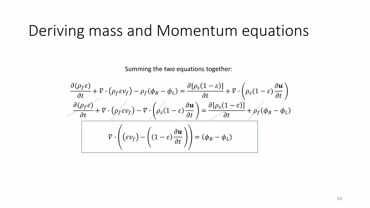
Deriving mass and Momentum equations

63

𝜕(𝜌𝑓휀)

𝜕𝑡+ 𝛻 ∙ 𝜌𝑓휀𝑣𝑓 − 𝜌𝑓 𝜙𝐵 − 𝜙𝐿 =

𝜕[𝜌𝑠 1 − 휀 ]

𝜕𝑡+ 𝛻 ∙ 𝜌𝑠(1 − 휀)

𝜕𝒖

𝜕𝑡

Summing the two equations together:

𝜕(𝜌𝑓휀)

𝜕𝑡+ 𝛻 ∙ 𝜌𝑓휀𝑣𝑓 − 𝛻 ∙ 𝜌𝑠 1 − 휀

𝜕𝒖

𝜕𝑡=𝜕 𝜌𝑠 1 − 휀

𝜕𝑡+ 𝜌𝑓 𝜙𝐵 − 𝜙𝐿

𝛻 ∙ 휀𝑣𝑓 − 1 − 휀𝜕𝒖

𝜕𝑡= 𝜙𝐵 − 𝜙𝐿

Biot Law

• According to a paper written in 1984 (that I do not have access too):

• Zienkiewicz, O. C., and T. Shiomi. "Dynamic behaviour of saturated porous media; the generalized Biotformulation and its numerical solution." International journal for numerical and analytical methods in geomechanics 8.1 (1984): 71-96.

64

휀 𝑣𝑓 −𝜕𝒖

𝜕𝑡= −𝐾𝛻𝑝

𝛻 ∙ 𝝈 = 0

Using BIOTS law to substitute…

65

𝛁 ∙ 𝝈 = 𝜇𝐺𝛻2𝒖 + (𝜇𝐺 + 𝜇λ)𝛻𝑒 + 𝛻𝑝 = 𝟎

(2𝜇𝐺 + 𝜇λ)𝛻2𝑒 = 𝛻2𝑝

66

𝜕𝒆

𝜕𝑡= 𝐾𝛻2𝑝 + 𝜙𝐵 − 𝜙𝐿

휀 𝛻 ∙ 𝑣𝑓 −𝜕𝒆

𝜕𝑡= −𝐾𝛻2𝑝

If volume dilation and hydraulic

conductivity are homogenous

𝜕𝒆

𝜕𝑡= 𝐾(2𝜇𝐺 + 𝜇λ)𝛻

2𝑒 + 𝜙𝐵 − 𝜙𝐿

Coefficient of consolidation