BMP Cost and Savings Study Update

A Guide to Data and Methods for Cost-Effectiveness Analysis of Urban Water Conservation Best Management Practices

July 2014 Update

California Urban Water Conservation Council

Conducted By:

Western Policy Research

171 Pier Avenue

Suite 256 Santa Monica, California 90405

Preface to the Revision This 2014 revision of the Cost and Savings Study is a stand alone revision for three topics addressed in prior versions of the study, as well as several conceptual topics identified in the 2005 study as known areas where future research is needed. These topics will be integrated into the Cost and Savings Study during the next revision to the study. The following topics have been revised from the 2005 Study:

• Large Landscape – Page 1 • High Efficiency Washers – Page 8 • Weather Based Irrigation Controllers (Residential) – Page 18

A new section for each of the following conceptual topics:

• Discount Rates – Page 29 • Savings Decay Over Time – Page 31 • Natural Replacement Rates – Page 35

Acknowledgements This project was supported by and prepared for the California Urban Water Conservation Council. CUWCC signatories that contributed to the original project fund include:

Alameda County Water District City of Santa Monica Contra Costa Water District East Bay Municipal Utility District Kern County Water Agency Los Angeles Department of Water and Power Metropolitan Water District of Southern California San Diego County Water Authority Santa Clara Valley Water District

Funding for the revisions has been provided by: California Water Foundation – Resource Legacy Fund CUWCC and Western Policy Research appreciate the time and energy contributed by the Project Advisory Committee of the Research and Evaluation Committee:

Mark Graham - Research and Evaluation Chair, Metropolitan Water District Matt Dickens - Research and Evaluation Vice Chair, Valencia Water Bill Jacoby California Water Foundation Ronnie Cohen California Water Foundation Bill Maddaus, Maddaus Water Management Carrie Pollard, Sonoma County Water Agency Greg Bundesen, Sacramento Suburban Water District John Koeller, Koeller & Company Joe Berg, Municipal Water District of Orange County Matt Heberger, Pacific Institute Mike Hazinski, East Bay Municipal Utility District Sofia Marcus, Los Angeles Department of Water and Power

Additional committee members and contributors to this revision include:

Amy Talbot, Regional Water Authority Richard Harris, East Bay Municipal Utility District Chris Brown, California Urban Water Conservation Council Gregory Weber, California Urban Water Conservation Council Luke Sires, California Urban Water Conservation Council

Much of the savings and cost information in this document has been published previously in other sources. Though we are grateful to build on this previous work, the errors that remain are our own.

LARGE LANDSCAPE PROGRAMS: AN UPDATE ABOUT COSTS AND SAVINGS

1. BACKGROUND Although reducing wasteful irrigation is a high priority in both the residential and non-residential sectors, the large landscape Best Management Practice (BMP) is largely meant for the non-residential sector. To promote water-use efficiency, water suppliers are required to establish water budgets for landscapes with dedicated irrigation meters. They are then also required to report discrepancies to the property owner between their water budget and actual use by billing period, and offer technical assistance and financial incentives to bring the two in line in case actual use exceeds the budget by more than 20%. For large landscapes on mixed-use meters, water suppliers are required to devise a strategy for first identifying such accounts, second offering them surveys to uncover irrigation-system deficiencies, and third offering them technical assistance and financial incentives to fix these deficiencies.1

Wasteful irrigation can result from many interlinked causes. These include bad hydro zoning of plant materials, improper pressure regulation, irrigation system leaks, unsuitable sprinkler heads, damaged (clogged, sunken, tilted or misaligned) sprinkler heads, poor distribution uniformity, improper irrigation scheduling leading to water loss due to runoff or deep percolation past the root zone, and finally improper horticultural practices.

Landscape experts agree that to eliminate wasteful irrigation requires a system-wide strategy. Simply retrofitting old hardware, such as sprinkler heads or irrigation controllers may not yield significant success without behavior modification. However, while the goal of large landscape programs is clear, it is difficult to advocate for a uniform, agreed-upon package of steps for getting there. Accordingly, water suppliers generally select and emphasize one or more of the following steps as a way of promoting water use efficiency in the large landscape sector. These include:

• Landscaper education and certification • Education of property owners • Establishment of water budgets2 and tracking of actual use (that is, benchmarking of actual

versus efficient use during each billing cycle)

1 Whitcomb, J., Kah, G. and W.C. Willig, BMP 5 Handbook: A Guide to Implementing Large Landscape Conservation Programs as Specified in Best Management Practice 5, a report prepared for the California Urban Water Conservation Council, 1999. 2 The analytic framework laid out in the Model Water Efficient Landscape Ordinance AB 1881 and associated budget calculator can aid water suppliers in establishing water budgets for their large landscapes (www.water.ca.gov/wateruseefficiency/landscapeordinance).

1

• Irrigation equipment retrofits (including sprinkler heads, irrigation controllers, pressure regulation, drip irrigation, etc.)

• Meter retrofits (advanced metering infrastructure (AMI) systems3, etc.) • Landscape re-design (promoting proper hydro-zoning, native vegetation, turf removal) • Promoting recycled water • Conservation-oriented rate structures (preferably tied to water budgets)

With respect to landscaper education and certification, landscape contractors are required to obtain a state contractor’s license to operate in California if they wish to undertake projects exceeding $500 in labor and material costs combined (www.cslb.ca.gov). Applicants have to demonstrate adequate work experience as part of the application process, although the problem of unlicensed contractors remains significant. For more specialized tasks, such as, installation and repair of irrigation systems, landscape auditing, landscape water management, etc., clients often demand additional certifications. The key organizations that implement these additional education and certification programs in California include the Irrigation Association, the California Landscape Contractors Association, and the Sonoma-Marin Qualified Water Efficient Landscaper (QWEL) program. These programs are also WaterSense endorsed (www.epa.gov/watersense/outdoor/cert_programs). Water suppliers often leverage these programs to improve landscaper education in their service area.

2. WATER SAVINGS Estimation of water savings from large landscape programs poses difficult challenges because of the interlinked nature of the various components that comprise these programs, which makes savings highly path dependent, that is, dependent upon the sequence in which various program components are rolled out. For example, the impact of equipment retrofit programs may differ if a conservation-oriented rate structure has been in place for many moons prior to the implementation of these retrofit programs, owing to the pro-efficiency behavioral change likely generated by the rate structure. Similarly, the impact of education programs will likely differ if they are run independently or concomitantly with other retrofit programs or with conservation-oriented rate structures, etc. While several studies have evaluated the impact of one or more components of a large landscape conservation program, virtually none have addressed the question of path dependence in a comprehensive way.

How then does one estimate savings from large landscape programs in the aggregate, unaffected by path dependence biases? An answer to this question perhaps lies in a key feature of all large landscape programs, namely, the requirement to establish water budgets. Since the large landscape BMP requires that water suppliers establish water budgets and track and inform property owners about how they are doing relative to their budgets, this then provides an approach for both managing and evaluating a large landscape program. Under this approach it is not necessary to quantify how a site achieved water savings, or to allocate these savings to the myriad steps that may have been taken under the auspices of a large landscape program. The alternative approach would be to aggregate savings across all program

3 While AMI systems have broader benefits, they are particularly useful for implementing budget based programs. The early warning provided by AMI systems allows landscapers and property managers to be much more proactive.

2

components: This, however, is unlikely to yield reasonable program-wide savings estimates until they are trued-up with actual use and the water budget.

Given the difficulty in making a bottoms-up approach work, why then bother with such an approach at all? Well, if the goal is not limited to estimating overall savings but also includes questions about program design and maximization of program cost-effectiveness then it is important to have a rank ordering of large-landscape program components according to their level of effectiveness and cost-effectiveness. Therefore, in reality both the top-down (that is, budget based) and the bottom-up (that is, program component based) approaches are necessary. We review information pertinent to both approaches next.

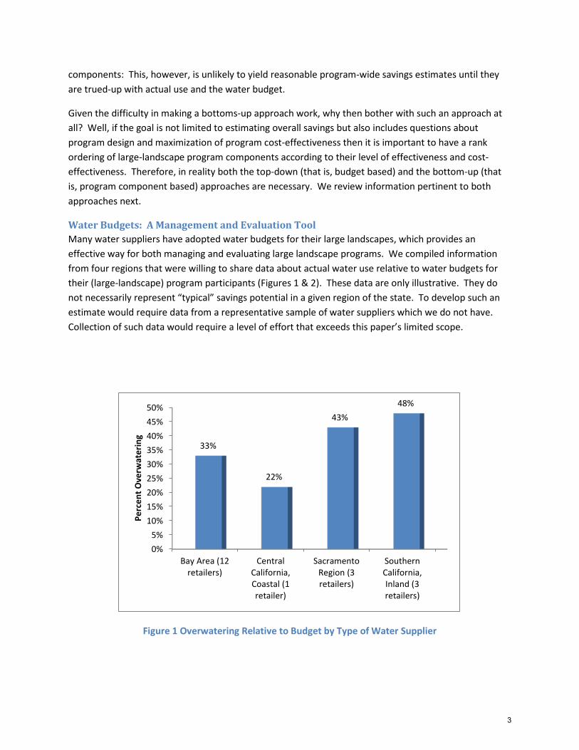
Water Budgets: A Management and Evaluation Tool Many water suppliers have adopted water budgets for their large landscapes, which provides an effective way for both managing and evaluating large landscape programs. We compiled information from four regions that were willing to share data about actual water use relative to water budgets for their (large-landscape) program participants (Figures 1 & 2). These data are only illustrative. They do not necessarily represent “typical” savings potential in a given region of the state. To develop such an estimate would require data from a representative sample of water suppliers which we do not have. Collection of such data would require a level of effort that exceeds this paper’s limited scope.

Figure 1 Overwatering Relative to Budget by Type of Water Supplier

0%5%

10%15%20%25%30%35%40%45%50%

Bay Area (12retailers)

CentralCalifornia,Coastal (1retailer)

SacramentoRegion (3retailers)

SouthernCalifornia,Inland (3retailers)

33%

22%

43% 48%

Perc

ent O

verw

ater

ing

3

These data convey two important points that most professionals involved with large landscape programs will find unsurprising. First, there is probably wide variation in the level of over-irrigation taking place across California’s landscapes with hotter, inland regions exhibiting greater levels of inefficiency. If broadly true, this is especially worrisome since a great deal of future growth is expected to occur in these hotter, inland regions of California. Figure 1 also challenges conventional wisdom to some extent because the Bay Area, normally associated with low outdoor use, does not appear notably efficient. Second, over-irrigation is not equally prevalent across different types of large landscapes (Figure 2). Professionally managed sites such as golf courses and cemeteries are usually quite efficient. The most inefficiently managed landscapes are usually found in commercial properties and home owner associations (HOAs).

Figure 2 Overwatering Relative to Budget by Site Type (Central California, Coastal Supplier)

Water Savings Associated with Components of Large Landscape Programs Several studies have evaluated the impact of landscape education, rates, horticultural practices, turf removal, and equipment retrofits on water use of large landscapes. We review the results of these studies next.

The impact of landscape education on compliance with water budgets was evaluated in Orange County, California in a 2004 study4. The education component was targeted at landscape contractors and

4 Chesnutt, T.W. et al., Evaluation of the Landscape Performance Certification Program, a report prepared for the Municipal Water District of Orange County, Metropolitan Water District of Southern California, and the US Bureau of Reclamation, 2004

0%

10%

20%

30%

40%

50%

60%

70%

80% 73%

0% 8%

0%

23%

34%

10% 5%

Perc

ent O

verw

ater

ing

4

property managers at home-owner associations (HOAs). The results were based on the experience of 47 HOAs that had participated in the program up to that point. The impact evaluation concluded that early participants in the program reduced their water demand by 9%, later participants by 20% (the difference between early and later participants was not explained).

Several studies are available that examine the impact of budget-based rates on large landscape water use. An early study, published in 1997 showed that tiered rates tied to landscape water budgets can reduce irrigation demand by 20-37%5. More recent journal articles have fleshed out further how water agencies can go about setting budget-based tiered rates6.

Another early 1997 study examined the relative impact of budget-based rates, education and outreach, and advanced horticultural practices on large landscape water use7. This study showed that education and outreach are critical components without which budget-based rates may only generate meagre savings. However, neither budget-based tiered rates nor outreach was able to completely eliminate inefficient irrigation until advanced horticultural practices were also introduced into the maintenance routines followed in the test landscapes. Prior to the evaluation these test landscapes were using over 100 inches of water per year. After all the interventions were put in place, irrigation was halved and wasteful irrigation was almost completely eliminated. This study showed that rates, education, and outreach caused irrigation demand to drop by roughly 30% relative to the baseline, and superior maintenance and horticultural practices, by an additional 20%.

Many studies in the past have evaluated the impact of turf removal. A relatively recent evaluation of Xeriscape in Nevada found that annual household water demand dropped by 30% after turf landscapes were replaced with Xeriscape8. Another evaluation in Southern California found that turf removal reduced annual water demand by roughly 24% in the participating commercial sites and by 18% in the participating residential sites9.

With respect to equipment retrofits, several studies have evaluated the impact of weather-based irrigation controllers (WBIC) in commercial settings. For example, a study completed for Los Angeles Department of Water and Power estimated the impact of two different WBIC models: one model

5 Pekelney, D. and T. W. Chesnutt, Landscape Water Conservation Programs: Evaluation of Water Budget Based Rate Structures, a report prepared for the Metropolitan Water District of Southern California, 1997. 6 Mayer, P., et al., Water Budgets and Rate Structures: Innovative Management Tools, Journal AWWA, Volume 100:5, 2008. Hildebrand, M., et al., Water Conservation Made Legal: Water Budgets and California Law, Journal AWWA, Volume 101:4, 2009. 7 Pagano, D.D., Barry, J. and Western Policy Research, Efficient Turf Grass Management: Findings from the Irvine Spectrum Water Conservation Study, a report prepared for the Metropolitan Water District of Southern California, 1997. 8 Sovocool, K., Xeriscape Conversion Study: Final Report, a report prepared for the Southern Nevada Water Authority and the US Bureau of Reclamation, 2005. 9 Metropolitan Water District of Southern California, California Friendly Turf Replacement Incentive Program Southern California: Final Project Report, 2013 (see Appendix E).

5

reduced irrigation demand by roughly 17%; the other by 28% in landscapes with dedicated meters10. A study completed in Irvine, California estimated that WBICs caused irrigation demand to drop by 22% in the commercial landscapes that participated in the retrofit program11. A large-landscape retrofit study completed in San Diego detected a drop in irrigation of between 24-48% after WBIC retrofits12. At present there are nozzle and pressure regulator retrofit evaluations underway that will add to our knowledge about yet another type of retrofit.

This quick review of the prior literature demonstrates the challenge of a bottoms-up approach. Many of these earlier studies are based on small samples, often samples exhibiting egregious levels of water waste. If a water supplier were contemplating designing a large-landscape program consisting of components such as, landscaper certification, conservation rates, water budgets and some hardware retrofits (e.g., WBICs) they would considerably overstate their program’s savings potential if they simply aggregated each component’s savings based on published research. It is therefore imperative that savings derived from a bottoms-up approach be trued up against actual water use and the water budget.

3. COSTS Costing out a large landscape program is difficult because it depends on a program’s overall size and on which components are included under its auspices.

Large landscape conservation programs can involve sizeable setup costs, such as designing a reporting system that delivers a comparison of actual and budgeted water use every billing period to large landscape property owners and/or their landscape contractors; setup of budget-based water rates; setup of education programs for landscape contractors and property owners, etc. By forming partnerships, water suppliers can help to reduce the impact of many of these setup costs.

Large landscape programs also involve costs that are more site specific, such as, the cost of hardware retrofits, the cost of landscape area measurement, the cost of site audits, etc. These costs can be expected to more or less scale with the number of landscape accounts included in a large landscape program.

Finally, the longevity of water savings may be directly related to ongoing education and outreach efforts undertaken by a water supplier. The churn in landscape contractors and property owners requires an ongoing commitment on the part of the water supplier to detect an unusual spike in water demand and then do something about it. Unless staff time is properly allocated for this purpose, savings may well erode over time. Maintaining efficient outdoor water use requires vigilance first and foremost, which boils down to behavior mainly. Large landscape programs generally continue to incur costs even for

10 Bamezai, A., LADWP Weather-Based Irrigation Controller Pilot Study, a report prepared for the Los Angeles Department of Water and Power, 2004. 11 Chesnutt, T.W. and D. Holt, Commercial ET-Based Irrigation Controller Water Savings Study, a report prepared for the Irvine Ranch Water District and the US Bureau of Reclamation, 2006. 12 ECONorthwest, Embedded Energy in Water Pilot Programs Impact Evaluation, a report prepared for the California Public Utilities Commission, 2011.

6

sites already in the program, and these must be properly accounted for while testing for program cost-effectiveness and for estimating financial outlays required for implementing a large landscape program.

Anecdotal evidence suggests that to develop water budgets can cost anywhere between $200-300 per site, with roughly an ongoing $100 per year expense for transmitting the actual-versus-budget comparison for every billing cycle. Large landscape audits can cost up to $1,500 per site depending on the thoroughness of the audit, which may include one or more of the following elements: (1) review of consumption history; (2) interview of landscape contractor and/or property owner; (3) pressure testing; (4) examination of sprinkler heads; (5) distribution uniformity testing; (6) leak testing; (7) irrigation schedule review; and (8) suggestions about plant palette modifications.

Water suppliers also offer financial incentives to promote hardware retrofits. Data collected from the Metropolitan Water District of Southern California shed light on the current level of incentives being offered for the most common types of hardware retrofits. These include: (1) $25 per station for a smart irrigation controller; (2) $7 per large rotary nozzle; (3) $3 per rotary multi-stream nozzle, etc. These types of data can be utilized to cost out the hardware retrofit element of large landscape programs.

4. EFFECTIVE LIFE The effective life of water savings generated by a large landscape program depends upon which particular programmatic component one is discussing. Certain components, such as turf removal and budget-based conservation rates are likely to have long lived, almost permanent effects. On the other hand, savings generated by water budgets, landscape audits, even hardware retrofits may erode over time because of the churn in landscape contractors and property owners. It is very important for water suppliers to maintain an ongoing education and outreach program to deal with this churn and thereby prolong the effectiveness of their large landscape programs.

Since water budgets are an integral component of most large landscape programs, water suppliers do not have to guess at their program’s level of effectiveness. Tracking actual and budgeted use offers ample real-time information about how much water their large landscape program is generating and whether these savings are holding or eroding over time. With an effective education and outreach program, there is no reason in principle why these savings could not be long lived.

5. THE CHALLENGE AHEAD Existence of water budgets presents a golden opportunity for addressing many questions about large landscape programs. If large landscape programmatic data could be collected from a representative sample of water suppliers several of the following questions could be addressed. These include:

• How much over irrigation is at present occurring in different parts of the state? • How does over irrigation vary by site type? • How long does it take for actual use to get ratcheted down to match budgeted use? • What level of ongoing education and outreach is necessary to maintain program effectiveness? • Which programmatic components appear to be the most effective?

7

RESIDENTIAL CLOTHES WASHERS: AN UPDATE ABOUT COSTS & SAVINGS

1. BACKGROUND Water suppliers that have signed the Council’s Memorandum of Understanding (MOU) must either provide incentives or institute ordinances that require the purchase of high-efficiency clothes washers meeting an average Water Factor of 5.0. If WaterSense adopts a lower Water Factor standard in the future, MOU signatories must comply with this lower standard. This is how the clothes washer Best Management Practice (BMP) is described in the MOU.

Several end-use studies in single-family settings have shown that clothes washing accounts for indoor water demand that is second only to toilets. Therefore, improving clothes washer efficiency has been a prominent goal among water suppliers interested in promoting conservation. Water suppliers have adopted a two-pronged approach for achieving this goal. They have advocated for mandatory water-use efficiency appliance standards; and they have implemented rebate programs to incentivize the retrofit of old inefficient washers.

2. RESIDENTIAL CLOTHES WASHER APPLIANCE STANDARDS Residential clothes washers have been subject to Federal energy efficiency standards since 19881. For example, The National Appliance Energy Conservation Act of 1987 states that “all rinse cycles of clothes washers shall include an unheated water option…” for clothes washers manufactured after January 1, 1988. This early rudimentary energy standard became progressively refined, appearing in the form of an “Energy Factor” metric in 1994, a “Modified Energy Factor” metric in 2004, and now an “Integrated Modified Energy Factor” for washers manufactured from 2015 onward. The aim of these refinements has been to create an energy-efficiency metric that first normalizes energy use for washer tub volume, and, second, captures total energy used by the washer/dryer combination. A washer uses energy to both run the washing machine and to supply the hot water. However, a washer that squeezes out more moisture from a load of wash reduces subsequent drying energy, an aspect of washer design that the early “Energy Factors” failed to capture but were subsequently included in the definition of “Modified Energy Factors.” The latest “Integrated Modified Energy Factor” is the most comprehensive metric developed to date, capturing energy used by hot water in an average wash cycle, the washer’s own electric energy consumption including when it is in stand-by mode, and drying energy. A higher energy factor indicates a more energy-efficient washing machine.

While water-use efficiency of clothes washers has also increased over time as a byproduct of the quest for greater energy efficiency (for example, through the development of front-loading, horizontal axis washing machines), water conservation professionals and environmentalists both have advocated for explicit water efficiency standards for some time. In response, the Federal government adopted in 2007 a metric called “Water Factor,” which residential clothes washers must comply with if manufactured 1 http://www1.eere.energy.gov/buildings/appliance_standards/product.aspx/productid/39#historicalinformation

8

after January 1, 2011. A washing machine’s Water Factor indicates the gallons of water required per cycle per cubic foot of washer tub volume. Lower water factors indicate greater water-use efficiency. Federal residential clothes washer standards were again revised in 2012. These latest, more stringent standards will go into effect in two phases, in 2015 and then in 2018. The metric used to capture water use efficiency, has also been revised and now is called the “Integrated Water Factor.” “Water Factor” was based on water usage of the cold wash/cold rinse cycles of a washing machine, while the new “Integrated Water Factor” evaluates water consumption across all cycles.2

In the clothes washer/dryer context, the tight linkage between water and energy efficiency has caused many water and energy utilities to enter into cost-sharing partnerships for the implementation of HECW rebate and retrofit programs.

Tables 1 and 2 include the current, the 2015, and the 2018 efficiency standards applicable to residential clothes washers.3

Table 1 Residential Clothes Washers: Current Energy and Water Efficiency Standards

Product Category Minimum Modified

Energy Factor (ft3/kWh/cycle)

Maximum Water Factor (gal/cycle/ft3)

1. Top-loading, Compact (less than 1.6 ft3 capacity) 0.65a Not Applicable

2. Top-loading, Standard (1.6 ft3 or greater capacity) 1.26b 9.5c

3. Top-loading, Semi-automatic Not Applicabled Not Applicable

4. Front-loading 1.26b 9.5c,e

5. Suds-saving Not Applicablec,d Not Applicable a For clothes washers manufactured after January 1, 2004. b For clothes washers manufactured after January 1, 2007. c For clothes washers manufactured after January 1, 2011. d Must have an unheated rinse water option. e Applies to standard-size front-loading clothes washers only.

2 Details about residential clothes washer standards and test procedures can be found at the Department of Energy’s website cited in earlier footnote. 3 Commercial clothes washers are subject to slightly different energy and water efficiency standards. More details about commercial clothes washers can be found in the following report: Bamezai, A., Coin-Operated Clothes Washers in Laundromats and Multi-Family Buildings: Assessment of Water Conservation Potential, a report prepared for the California Urban Water Conservation Council, 2012.

9

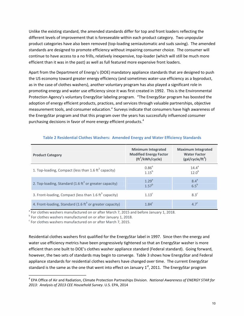
Unlike the existing standard, the amended standards differ for top and front loaders reflecting the different levels of improvement that is foreseeable within each product category. Two unpopular product categories have also been removed (top-loading semiautomatic and suds saving). The amended standards are designed to promote efficiency without impairing consumer choice. The consumer will continue to have access to a no frills, relatively inexpensive, top-loader (which will still be much more efficient than it was in the past) as well as full featured more expensive front loaders.

Apart from the Department of Energy’s (DOE) mandatory appliance standards that are designed to push the US economy toward greater energy efficiency (and sometimes water-use efficiency as a byproduct, as in the case of clothes washers), another voluntary program has also played a significant role in promoting energy and water use efficiency since it was first created in 1992. This is the Environmental Protection Agency’s voluntary EnergyStar labeling program. “The EnergyStar program has boosted the adoption of energy efficient products, practices, and services through valuable partnerships, objective measurement tools, and consumer education.” Surveys indicate that consumers have high awareness of the EnergyStar program and that this program over the years has successfully influenced consumer purchasing decisions in favor of more energy efficient products.4

Table 2 Residential Clothes Washers: Amended Energy and Water Efficiency Standards

Product Category Minimum Integrated

Modified Energy Factor (ft3/kWh/cycle)

Maximum Integrated Water Factor (gal/cycle/ft3)

1. Top-loading, Compact (less than 1.6 ft3 capacity) 0.86a 1.15b

14.4a 12.0b

2. Top-loading, Standard (1.6 ft3 or greater capacity) 1.29a 1.57b

8.4a 6.5b

3. Front-loading, Compact (less than 1.6 ft3 capacity) 1.13c 8.3c

4. Front-loading, Standard (1.6 ft3 or greater capacity) 1.84c 4.7c a For clothes washers manufactured on or after March 7, 2015 and before January 1, 2018. b For clothes washers manufactured on or after January 1, 2018. c For clothes washers manufactured on or after March 7, 2015.

Residential clothes washers first qualified for the EnergyStar label in 1997. Since then the energy and water use efficiency metrics have been progressively tightened so that an EnergyStar washer is more efficient than one built to DOE’s clothes washer appliance standard (Federal standard). Going forward, however, the two sets of standards may begin to converge. Table 3 shows how EnergyStar and Federal appliance standards for residential clothes washers have changed over time. The current EnergyStar standard is the same as the one that went into effect on January 1st, 2011. The EnergyStar program

4 EPA Office of Air and Radiation, Climate Protection Partneships Division. National Awareness of ENERGY STAR for 2013: Analysis of 2013 CEE Household Survey. U.S. EPA, 2014

10

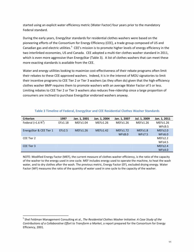
started using an explicit water efficiency metric (Water Factor) four years prior to the mandatory Federal standard.

During the early years, EnergyStar standards for residential clothes washers were based on the pioneering efforts of the Consortium for Energy Efficiency (CEE), a trade group composed of US and Canadian gas and electric utilities.5 CEE’s mission is to promote higher levels of energy efficiency in the two interlinked economies, US and Canada. CEE adopted a multi-tier clothes washer standard in 2011, which is even more aggressive than EnergyStar (Table 3). A list of clothes washers that can meet these more exacting standards is available from the CEE.

Water and energy utilities looking to maximize cost-effectiveness of their rebate programs often limit their rebates to these CEE-approved washers. Indeed, it is in the interest of MOU signatories to limit their incentive programs to CEE Tier 2 or Tier 3 washers (as they often do) given that the high-efficiency clothes washer BMP requires them to promote washers with an average Water Factor of 5 or less. Limiting rebates to CEE Tier 2 or Tier 3 washers also reduces free-ridership since a large proportion of consumers are inclined to purchase EnergyStar endorsed washers anyway.

Table 3 Timeline of Federal, EnergyStar and CEE Residential Clothes Washer Standards

Criterion 1997 Jan. 1, 2001 Jan. 1, 2004 Jan. 1, 2007 Jul. 1, 2009 Jan. 1, 2011 Federal (>1.6 ft3) EF≥1.18 MEF≥1.04 MEF≥1.26 MEF≥1.26

MEF≥1.26

MEF≥1.26 WF≤9.5

EnergyStar & CEE Tier 1 EF≥2.5 MEF≥1.26 MEF≥1.42 MEF≥1.72 WF≤8.0

MEF≥1.8 WF≤7.5

MEF≥2.0 WF≤6.0

CEE Tier 2 MEF≥2.2 WF≤4.5

CEE Tier 3 MEF≥2.4 WF≤4.0

Note: Current criteria and standards are in shaded boxes. Modified Energy Factor (MEF), the current measure of clothes washer efficiency, is the ratio NOTE: Modified Energy Factor (MEF), the current measure of clothes washer efficiency, is the ratio of the capacity of the washer to the energy used in one cycle. MEF includes energy used to operate the machine, to heat the wash water, and to dry clothes after the wash. The previous metric, Energy Factor (EF), excluded drying energy. Water Factor (WF) measures the ratio of the quantity of water used in one cycle to the capacity of the washer.

5 Shel Feldman Management Consulting et al., The Residential Clothes Washer Initiative: A Case Study of the Contributions of a Collaborative Effort to Transform a Market, a report prepared for the Consortium for Energy Efficiency, 2001.

11

3. WATER SAVINGS

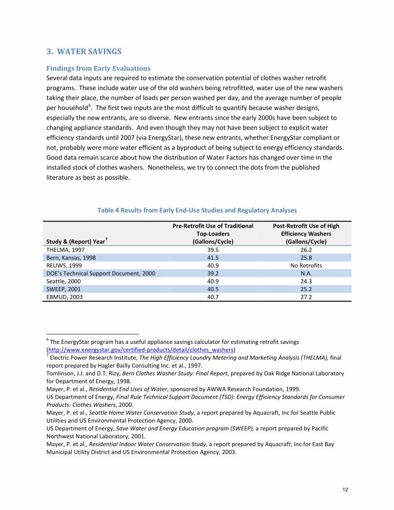
Findings from Early Evaluations Several data inputs are required to estimate the conservation potential of clothes washer retrofit programs. These include water use of the old washers being retrofitted, water use of the new washers taking their place, the number of loads per person washed per day, and the average number of people per household6. The first two inputs are the most difficult to quantify because washer designs, especially the new entrants, are so diverse. New entrants since the early 2000s have been subject to changing appliance standards. And even though they may not have been subject to explicit water efficiency standards until 2007 (via EnergyStar), these new entrants, whether EnergyStar compliant or not, probably were more water efficient as a byproduct of being subject to energy efficiency standards. Good data remain scarce about how the distribution of Water Factors has changed over time in the installed stock of clothes washers. Nonetheless, we try to connect the dots from the published literature as best as possible.

Table 4 Results from Early End-Use Studies and Regulatory Analyses

Study & (Report) Year7

Pre-Retrofit Use of Traditional Top-Loaders

(Gallons/Cycle)

Post-Retrofit Use of High Efficiency Washers

(Gallons/Cycle) THELMA, 1997 39.5 26.2 Bern, Kansas, 1998 41.5 25.8 REUWS, 1999 40.9 No Retrofits DOE’s Technical Support Document, 2000 39.2 N.A. Seattle, 2000 40.9 24.3 SWEEP, 2001 40.5 25.2 EBMUD, 2003 40.7 27.2

6 The EnergyStar program has a useful appliance savings calculator for estimating retrofit savings (http://www.energystar.gov/certified-products/detail/clothes_washers) 7 Electric Power Research Institute, The High Efficiency Laundry Metering and Marketing Analysis (THELMA), final report prepared by Hagler Bailly Consulting Inc. et al., 1997. Tomlinson, J.J. and D.T. Rizy, Bern Clothes Washer Study: Final Report, prepared by Oak Ridge National Laboratory for Department of Energy, 1998. Mayer, P. et al., Residential End Uses of Water, sponsored by AWWA Research Foundation, 1999. US Department of Energy, Final Rule Technical Support Document (TSD): Energy Efficiency Standards for Consumer Products: Clothes Washers, 2000. Mayer, P. et al., Seattle Home Water Conservation Study, a report prepared by Aquacraft, Inc.for Seattle Public Utilities and US Environmental Protection Agency, 2000. US Department of Energy, Save Water and Energy Education program (SWEEP), a report prepared by Pacific Northwest National Laboratory, 2001. Mayer, P. et al., Residential Indoor Water Conservation Study, a report prepared by Aquacraft, Inc.for East Bay Municipal Utility District and US Environmental Protection Agency, 2003.

12

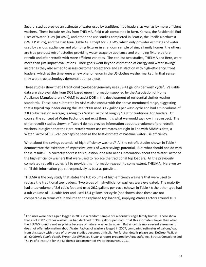
Several studies provide an estimate of water used by traditional top loaders, as well as by more efficient washers. These include results from THELMA, field trials completed in Bern, Kansas, the Residential End Uses of Water Study (REUWS), and other end use studies completed in Seattle, the Pacific Northwest (SWEEP study), and the Bay Area (Table 4). Except for REUWS, which only provides estimates of water used by various appliances and plumbing fixtures in a random sample of single family homes, the others are true pre-post retrofit studies providing water usage by appliance and plumbing fixture before retrofit and after retrofit with more efficient varieties. The earliest two studies, THELMA and Bern, were more than just impact evaluations. Their goals went beyond estimation of energy and water savings insofar as they also aimed to assess customer acceptance and satisfaction with high-efficiency, front loaders, which at the time were a new phenomenon in the US clothes washer market. In that sense, they were true technology demonstration projects.

These studies show that a traditional top-loader generally uses 39-41 gallons per wash cycle8. Valuable data are also available from DOE based upon information supplied by the Association of Home Appliance Manufacturers (AHAM) to assist DOE in the development of residential clothes washer standards. These data submitted by AHAM also concur with the above-mentioned range, suggesting that a typical top loader during the late 1990s used 39.2 gallons per wash cycle and had a tub volume of 2.83 cubic feet on average, leading to a Water Factor of roughly 13.8 for traditional top loaders. Of course, the concept of Water Factor did not exist then. It is what we would say now in retrospect. The other retrofit studies shown in Table 4 do not provide information about tub volume of pre-retrofit washers, but given that their pre-retrofit water use estimates are right in line with AHAM’s data, a Water Factor of 13.8 can perhaps be seen as the best estimate of baseline water-use efficiency.

What about the savings potential of high efficiency washers? All the retrofit studies shown in Table 4 demonstrate the existence of impressive levels of water savings potential. But, what should one do with these results? To correctly address this question, one also needs information about the Water Factor of the high efficiency washers that were used to replace the traditional top loaders. All the previously completed retrofit studies fail to provide this information except, to some extent, THELMA. Here we try to fill this information gap retrospectively as best as possible.

THELMA is the only study that states the tub volume of high-efficiency washers that were used to replace the traditional top loaders: Two types of high-efficiency washers were evaluated. The majority had a tub volume of 2.6 cubic feet and used 26.2 gallons per cycle (shown in Table 4); the other type had a tub volume of 1.4 cubic feet and used 13.4 gallons per cycle (not shown since these are not comparable in terms of tub volume to the replaced top loaders), implying Water Factors around 10.1

8 End uses were once again logged in 2007 in a random sample of California’s single family homes. These show that as of 2007, clothes washer use had declined to 30.6 gallons per load. That this estimate is lower than what the REUWS found is not surprising because of natural washer turnover. But since this more recent assessment does not offer information about Water Factors of washers logged in 2007, comparing estimates of gallons/load from this study with those of previous studies becomes difficult. For further details please see: DeOreo, W.B. et al., California Single-Family Water Use Efficiency Study, a report prepared by Aquacraft, Inc., Stratus Consulting and The Pacific Institute for the California Department of Water Resources, 2011.

13

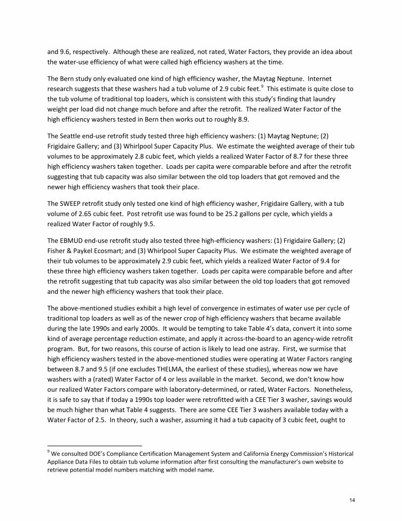
and 9.6, respectively. Although these are realized, not rated, Water Factors, they provide an idea about the water-use efficiency of what were called high efficiency washers at the time.

The Bern study only evaluated one kind of high efficiency washer, the Maytag Neptune. Internet research suggests that these washers had a tub volume of 2.9 cubic feet.9 This estimate is quite close to the tub volume of traditional top loaders, which is consistent with this study’s finding that laundry weight per load did not change much before and after the retrofit. The realized Water Factor of the high efficiency washers tested in Bern then works out to roughly 8.9.

The Seattle end-use retrofit study tested three high efficiency washers: (1) Maytag Neptune; (2) Frigidaire Gallery; and (3) Whirlpool Super Capacity Plus. We estimate the weighted average of their tub volumes to be approximately 2.8 cubic feet, which yields a realized Water Factor of 8.7 for these three high efficiency washers taken together. Loads per capita were comparable before and after the retrofit suggesting that tub capacity was also similar between the old top loaders that got removed and the newer high efficiency washers that took their place.

The SWEEP retrofit study only tested one kind of high efficiency washer, Frigidaire Gallery, with a tub volume of 2.65 cubic feet. Post retrofit use was found to be 25.2 gallons per cycle, which yields a realized Water Factor of roughly 9.5.

The EBMUD end-use retrofit study also tested three high-efficiency washers: (1) Frigidaire Gallery; (2) Fisher & Paykel Ecosmart; and (3) Whirlpool Super Capacity Plus. We estimate the weighted average of their tub volumes to be approximately 2.9 cubic feet, which yields a realized Water Factor of 9.4 for these three high efficiency washers taken together. Loads per capita were comparable before and after the retrofit suggesting that tub capacity was also similar between the old top loaders that got removed and the newer high efficiency washers that took their place.

The above-mentioned studies exhibit a high level of convergence in estimates of water use per cycle of traditional top loaders as well as of the newer crop of high efficiency washers that became available during the late 1990s and early 2000s. It would be tempting to take Table 4’s data, convert it into some kind of average percentage reduction estimate, and apply it across-the-board to an agency-wide retrofit program. But, for two reasons, this course of action is likely to lead one astray. First, we surmise that high efficiency washers tested in the above-mentioned studies were operating at Water Factors ranging between 8.7 and 9.5 (if one excludes THELMA, the earliest of these studies), whereas now we have washers with a (rated) Water Factor of 4 or less available in the market. Second, we don’t know how our realized Water Factors compare with laboratory-determined, or rated, Water Factors. Nonetheless, it is safe to say that if today a 1990s top loader were retrofitted with a CEE Tier 3 washer, savings would be much higher than what Table 4 suggests. There are some CEE Tier 3 washers available today with a Water Factor of 2.5. In theory, such a washer, assuming it had a tub capacity of 3 cubic feet, ought to

9 We consulted DOE’s Compliance Certification Management System and California Energy Commission’s Historical Appliance Data Files to obtain tub volume information after first consulting the manufacturer’s own website to retrieve potential model numbers matching with model name.

14

require only 7.5 gallons for a normal load instead of roughly 25 gallons that many early studies identified as the water requirement of high efficiency washers.

The latest end-use retrofit study completed in Albuquerque where CEE Tier 3 washers were used to retrofit the existing inefficient washers found that clothes washer use was down to 19.4 gallons per load after the retrofit.10 The study unfortunately fails to provide information about Water Factors of the CEE Tier 3 washers tested during the study to allow one to compare actual and theoretical use, but that is the kind of information that such end-use studies will have to generate in the future to allow planners to use their results prospectively.

Loads per Day Several end-use studies cited in Table 4 provide estimates of clothes washing frequency. For example, the REUWS estimated that a single-family household washes 0.99 loads per day on average, which translates into roughly 361 loads per year. However, data from DOE and AHAM suggest that average tub volumes have steadily increased over time, causing wash load frequency to correspondingly drop somewhat. For developing the latest residential clothes washer standards, DOE assumed that newer washers will be used to launder 295 loads per household per year.11 Changing tub volumes and washing frequency adds an extra layer of uncertainty to estimates of washer retrofit savings potential.

Predicting Savings Going Forward To reliably predict savings from clothes washer retrofit programs, water agencies need to take several steps. They need to collect granular data on age and characteristics of the old removed washers, as well as granular data about characteristics of the high-efficiency washers that were swapped in their place. Assumptions would still be required about the Water Factors of the old inefficient washers, as well as about the real-world water usage of the new washers (which may deviate somewhat from their rated Water Factors), but at least with granular data one can hope to arrive at more realistic savings estimates than blindly relying on percentage reduction factors drawn from previous studies: The high efficiency clothes washer world is changing much too fast for that strategy to work.

Having said that, though, water use efficiency of clothes washers does appear to have increased in chunks of a third. The earliest crop of efficient clothes washers with a Water Factor of 9.5 used roughly a third less water than traditional top loaders with a Water Factor of 13.8. The latest EnergyStar endorsed washers with a Water Factor of 6 use roughly a third less water than the early generation high efficiency washers. The washers designed to the most stringent CEE Tier 3 standard with a Water Factor of 4 will once again reduce water use by a third compared to an EnergyStar endorsed washer. Perhaps, some of these patterns can be exploited to model remaining conservation potential in the absence of granular data.

10 Aquacraft, Inc., Albuquerque Single Family Water Use Efficiency and Retrofit Study, a report prepared for Albuquerque Bernalillo County Water Utility Authority, 2011. 11 Department of Energy, Technical Support Document: Energy Efficiency Program for Consumer Products and Commercial and Industrial Equipment: Residential Clothes Washers, 2012.

15

Periodic analysis of washer market data that AHAM and the Federal government collect12, utility sponsored household saturation surveys and end-use studies will also be required to pin down how the distribution of Water Factors is changing over time in the installed stock of clothes washers.

4. COSTS While developing its amended standards for residential clothes washers, DOE collected extensive retail price data in 2009. These data show that price is positively related to energy efficiency, which translates into a higher price for front loaders since, on average, they are also more efficient than top loaders. Retail prices for top loaders were found to average $636 with a range of $319-$1,259. For front loaders, retail price averaged $1,041 with a range of $519-$2,449. Given the relationship between price and energy efficiency, it is possible to find many lower-end front loaders that are competitively priced relative to higher end top-loaders.13 DOE’s analyses are supported by another study from the American Council for an Energy Efficient Economy (ACEEE) based on Consumer Reports, which examines trends in clothes washer retail prices over time.14 This second study shows that font loader prices have been dropping much faster over time as washer-manufacturers ramp up scale of front-loader production. Low-price point front loaders have already become very competitive with top-loaders.

5. WASHER LIFE The Bern study and more recent data submitted by AHAM to DOE (Technical Support Document, 2012), cited earlier, suggest that a clothes washer’s average life is roughly 14 years. This is what California water suppliers have also generally assumed in their planning analyses. However, water agencies generally assume a constant risk of failure, which works out to roughly 7.1% per year (from an average assumed life of 14 years). A constant risk of failure implies that if one started with a stock of washers in a base year, by the first following year 7.1% would have failed, by the second following year, a total of 13.7% of the original stock would have failed, and so on. After 14 years, roughly 36% of the original stock would still be functioning, 64% would have failed. Data from the 2009 Residential Energy Consumption Survey (RECS) and also from the Bern study suggest that washer annual failure rate is probably not constant over time, being low initially, peaking at mid-life, stabilizing afterwards. The RECS data suggest that saturation of high-efficiency clothes washers may be increasing faster than what our traditional turnover models predict.

What this means in practice is that natural turnover can be expected to raise clothes washer efficiency at a slightly faster rate than traditionally predicted by code-savings models. However, to not assume constant failure risk requires having data about the distribution of age in the installed stock of clothes washers, which most water suppliers do not have. We therefore suggest that water suppliers continue to model natural washer turnover as they have in the past, but just be aware that water demand of the clothes washer end use may drop somewhat faster than what their natural-turnover models predict.

12 For example, the 2009 Residential Energy Consumption Survey (RECS) is a valuable source of information about changing saturation of EnergyStar washers in the US and its sub-regions. 13 Department of Energy, Technical Support Document: Energy Efficiency Program for Consumer Products and Commercial and Industrial Equipment: Residential Clothes Washers, 2012. 14 Mauer, J. et al., Better Appliances: An Analysis of Performance, Features, and Price as Efficiency Has improved, American Council for an Energy Efficient Economy, Report Number A132, 2013.

16

6. THE CHALLENGE AHEAD Reliable estimation of savings from clothes washer retrofit programs involves several challenges mainly because washers come in a variety of flavors. Appliance standards have changed significantly over time. The questions that remain unanswered and deserve a closer look include:

1. What is the distribution of Water Factors in the installed base of clothes washers? How is this changing over time as a result of natural turnover and active retrofit programs?

2. What are the impediments to collecting granular data about old washers removed and new washers installed in its place as a result of rebate and retrofit programs?

3. How does actual water use of a washer compare to what its Water Factor would predict? 4. How are other washer characteristics, such as tub volume changing over time, which might

influence washing frequency?

It is important that future evaluations of HECW retrofit programs, or even end use studies, collect granular data about the Water Factors of old washers removed and new ones retrofitted in their place. Otherwise, comparing results across studies becomes difficult. The CUWCC may also consider coordinating with AHAM, including purchasing AHAM’s data on behalf of Council members, to improve our information about clothes washer shipments over time and saturation of HECWs in California.

17

RESIDENTIAL WBICS: AN UPDATE ABOUT COSTS & SAVINGS

1. BACKGROUND Small scale, residential weather-based irrigation controllers (WBICs) first appeared on the scene during the late 1990s. Up until then weather-based irrigation controllers had only been available for commercial landscapes. These tended to be large, expensive systems. Since over half of residential consumption can be traced to outdoor use, a good chunk of it wasteful, water suppliers have been hungry for newer, effective tools to improve outdoor water use efficiency. As a result, residential WBICs have been extensively studied, with the first successful field trial completed in 2001. Many additional trials undertaken since then have added to the corpus of knowledge available about these devices. This paper’s objective is to take stock of what we know and identify gaps that still need to be filled.

Residential WBICs have come a long way since the 1990s when only 1 manufacturer was offering this technology. Today there are 20 manufacturers.1 WBICs can now be purchased easily at big box stores. Costs have dropped with scale and competition. Federal water use efficiency standards have been extended to cover WBICs through EPA’s WaterSense labeling program (analogous to the highly successful EnergyStar labeling program for promoting energy efficiency) which has brought a level of standardization to WBICs that would otherwise have been absent. Finally, water suppliers have actively promoted these devices through hefty rebate programs. Statewide in California, thousands of traditional irrigation timers have been retrofitted with WBICs. In sum, actions taken during the past 15 years by water suppliers, device manufacturers, landscape industry professionals and regulatory agencies has brought significant maturity to the WBIC market.

2. “SMART” CONTROLLER TECHNOLOGY AND PRODUCT CERTIFICATION WBICs are a subset of a larger group of irrigation controllers that are increasingly referred to as “smart” controllers. A key feature of “smart” controllers is that they can sense environmental conditions and tailor irrigation accordingly, without human intervention. Metrics used to capture these conditions, however, can vary. These conditions may include atmospheric metrics, such as temperature, solar radiation, wind speed, precipitation etc., for calculation of plant evapotranspiration rates, or direct soil moisture measurements. Apart from their sensing elements, “smart” controllers can also establish a more efficient baseline schedule from the get go, by allowing the user to incorporate information about landscape characteristics into the scheduling, such as plant type, soil type, slope, shade, etc. This can be a double-edged sword

1 Weather and Soil-Moisture Based Landscape Irrigation Scheduling Devices, Technical Review Report-4th Edition, 2012. (http://www.usbr.gov/waterconservation/docs/SmartController.pdf)

18

though; optimum scheduling of a “smart” controller requires a greater degree of scheduling knowledge. Users that blindly rely upon default built-in parameters can rob a “smart” controller of some of its ability to save water, hence the significant need for education and outreach to accompany WBIC retrofit programs.

In contrast, a traditional irrigation controller is no more than a timer, blindly irrigating a landscape some number of minutes per day based on the programmed schedule. A great deal of survey research shows that most homeowners change irrigation schedules infrequently, usually only seasonally, leading to wasteful irrigation (more on this topic later).

As mentioned earlier, “smart” controllers can include products that either sense atmospheric weather or soil-moisture content. This paper mainly focuses on the former, although where germane comparisons with soil-moisture based “smart” controllers have also been factored into the discussion.

Weather-based irrigation (“smart”) controllers are in turn divided into two broad groups:

1. Controllers with on-site weather sensors. One or more sensors (for example, for temperature, solar radiation, precipitation) feed weather data into the controller, which then calculates a plant evapotranspiration rate in real time, using this estimate to determine or modify a base irrigation schedule to reflect plant watering needs on any given day. These sensors may be designed to communicate with the controller through a wired connection or wirelessly. The sensors may be sold as part of a full package consisting of a controller, weather sensor and other accessories. Or, they may be sold as add-on units for existing compatible controllers, which become “smart” when coupled with the add-on unit.

2. Controllers that receive weather data from an off-site source. These controllers receive evapotranspiration data appropriate for their location from a central transmitting source, which are then used to create or adjust a baseline schedule programmed into the controller. These weather data may arrive via signals transmitted through the cellular phone spectrum, or through the internet via a home’s Wi-Fi network. Some manufacturers may charge an ongoing monthly fee to provide real-time weather data. Others may offer it free of charge, factoring in the cost of providing real-time weather information into the initial price.

In either type of WBIC, failure whether in the external sensor module or in the reception of real-time weather data causes the smart controller to revert to a default schedule (a baseline schedule or the last calculated schedule saved to memory). Landscapes continue to be watered, just not efficiently. Many residential WBICs can be controlled and programmed through a computer or smartphone based interface, with the controller relaying back system faults in case one develops. This 2-way communication capability was earlier available only among large

19

central irrigation systems found in commercial landscapes, but looks to become more widespread in residential settings as the “internet of things” slowly expands to cover WBICs.

Water suppliers interested in promoting WBICs through rebate and retrofit programs have looked for ways to ensure that products they incentivize meet some minimum efficacy standards where efficacy is defined as adequate irrigation with minimal runoff. Collaborative efforts in this regard between water suppliers and the irrigation industry led to a testing protocol called the Smart Water Applications Technologies (SWAT) initiative. Under this testing protocol smart controllers are evaluated using a “virtual landscape” designed to mimic different plant materials and soil types. Test results are published by consent of the manufacturers, but the test does not result in a “pass” or “fail” grade. It is up to the consumer and water suppliers to decide how to use the test results.

The Environmental Protection Agency’s (EPA) WaterSense labeling program, however, works a little bit differently. EPA’s WaterSense endorsement program is meant to raise water use efficiency just as the EnergyStar endorsement program has done for energy. The EPA has been endorsing WBICs as WaterSense compliant since 2012. EPA’s testing protocol is to a great degree based on the SWAT protocol, but it is administered separately and EPA does not publish its test results. Instead, WBICs are allowed to be advertised as WaterSense compliant if they meet minimum efficacy standards defined as 80% irrigation adequacy, less than 10% excess irrigation in any single landscape zone, and less than 5% excess irrigation when averaged across all landscape zones (per the “virtual” testing).

WaterSense endorsed WBICs must also include several additional design features. These include presence of non-volatile memory so that irrigation settings are not lost due to power outage, ability to notify the user when the device is not functioning in “smart” mode, ability to connect to a rain sensor, ability to easily accommodate utility-mandated watering restrictions, ability to ratchet down irrigation by a user-selected percentage to stay within a budget, etc. These controllers also allow the user to set parameters for plant type, soil type, slope, shade, etc. that are important for establishing an efficient baseline schedule.

By and large water suppliers limit their retrofit incentive programs to SWAT-tested or WaterSense compliant WBICs. Efforts to extend the WaterSense endorsement to qualifying soil-moisture based “smart” controllers are also underway.

3. WATER SAVINGS Several field trials have now been completed to evaluate water savings from WBIC retrofits. Many of the earlier studies, based on small samples, were mostly technology demonstration projects. These studies, while cited, have not otherwise been used for savings quantification2.

2 Addink, S., and Rodda, T. W., Residential Landscape Irrigation Study Using Aqua ET Controllers, 2002. Aquacraft, Performance Evaluation of WeatherTRAK Irrigation Controllers in Colorado, 2001 and 2002.

20

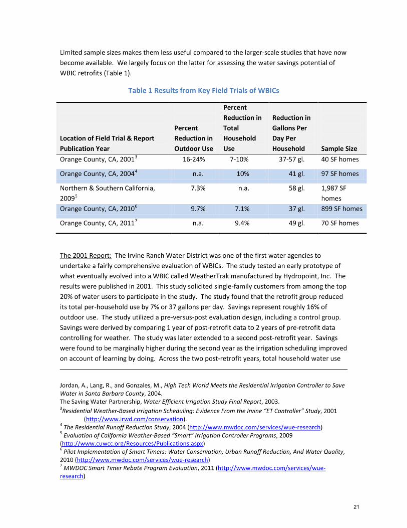
Limited sample sizes makes them less useful compared to the larger-scale studies that have now become available. We largely focus on the latter for assessing the water savings potential of WBIC retrofits (Table 1).

Table 1 Results from Key Field Trials of WBICs

Location of Field Trial & Report Publication Year

Percent Reduction in Outdoor Use

Percent Reduction in Total Household Use

Reduction in Gallons Per Day Per Household

Sample Size

Orange County, CA, 20013 16-24% 7-10% 37-57 gl. 40 SF homes

Orange County, CA, 20044 n.a. 10% 41 gl. 97 SF homes

Northern & Southern California, 20095

7.3% n.a. 58 gl. 1,987 SF homes

Orange County, CA, 20106 9.7% 7.1% 37 gl. 899 SF homes

Orange County, CA, 20117 n.a. 9.4% 49 gl. 70 SF homes

The 2001 Report: The Irvine Ranch Water District was one of the first water agencies to undertake a fairly comprehensive evaluation of WBICs. The study tested an early prototype of what eventually evolved into a WBIC called WeatherTrak manufactured by Hydropoint, Inc. The results were published in 2001. This study solicited single-family customers from among the top 20% of water users to participate in the study. The study found that the retrofit group reduced its total per-household use by 7% or 37 gallons per day. Savings represent roughly 16% of outdoor use. The study utilized a pre-versus-post evaluation design, including a control group. Savings were derived by comparing 1 year of post-retrofit data to 2 years of pre-retrofit data controlling for weather. The study was later extended to a second post-retrofit year. Savings were found to be marginally higher during the second year as the irrigation scheduling improved on account of learning by doing. Across the two post-retrofit years, total household water use

Jordan, A., Lang, R., and Gonzales, M., High Tech World Meets the Residential Irrigation Controller to Save Water in Santa Barbara County, 2004. The Saving Water Partnership, Water Efficient Irrigation Study Final Report, 2003. 3Residential Weather-Based Irrigation Scheduling: Evidence From the Irvine “ET Controller” Study, 2001

(http://www.irwd.com/conservation). 4 The Residential Runoff Reduction Study, 2004 (http://www.mwdoc.com/services/wue-research) 5 Evaluation of California Weather-Based “Smart” Irrigation Controller Programs, 2009 (http://www.cuwcc.org/Resources/Publications.aspx) 6 Pilot Implementation of Smart Timers: Water Conservation, Urban Runoff Reduction, And Water Quality, 2010 (http://www.mwdoc.com/services/wue-research) 7 MWDOC Smart Timer Rebate Program Evaluation, 2011 (http://www.mwdoc.com/services/wue-research)

21

was shown to have dropped by 41 gallons per day anticipating the findings of the later 2004 study. The 2001 study, however, was affected by significant self-selection bias. Compared to the control group, the treatment group was shown to have much lower wasteful irrigation prior to the WBIC retrofit. The 2001 study calculated that if WBICs had been installed in homes that resembled the control group (also selected from the top 20%) then water demand reductions would have been closer to 10% of total household use (or 24% of outdoor use or 57 gallons per household per day) instead of the estimated 7%. The study emphasized the need for proper targeting of wasteful irrigators to ensure a cost-effective program.

The 2004 Report: The 2001 “ET Controller” report was followed by what is informally called the “R3 Study” published in 2004. This study, also conducted in Irvine, California, showed that WBIC retrofits combined with customer education reduced water use by 10% or 41 gallons per household per day in the retrofitted homes. The 2004 study did not provide estimates of the percentage reduction in outdoor use, only total household use. However, under the reasonable surmise that roughly half of total use is accounted for by irrigation, a 10% reduction in total household use translates into a 20% reduction in outdoor use. This study also used a pre-versus-post retrofit comparison, including a control group. Once again the WBIC used in this study was an early prototype of what became WeatherTrak manufactured by Hydropoint, Inc. The R3 study also had other components such as evaluating the reduction in urban runoff as a result of WBIC retrofits, but those elements are not relevant to this paper. The “R3 Study” also targeted some of Irvine’s high water users, but the study does not clearly describe the percentile from which its retrofit group was drawn. The impact of selection bias on savings estimates also remains unexamined.

The 2009 Report: These two successful evaluations set the stage for scaling up of WBIC retrofit programs across California, establishing savings from larger samples, and most importantly comparing the efficacy of different WBIC models. A large multi-agency retrofit program was undertaken encompassing both northern and southern California. Study results were published in 2009. In southern California, very little attempt was made to target high water users. The northern California agencies supposedly did target high water users, but it’s not clear from the report how this was done. The 2009 study’s findings stand out as an outlier being much lower than the two studies that came before it, or the two since. The 2009 report only provides information about the reduction in outdoor use caused by WBIC retrofits. Estimates are derived by comparing 1 year of pre- and 1 year of post-retrofit water use controlling for weather differences between the two periods. The study design did not include a control group. The study also did not develop statistical billing-data models to estimate program impacts. Instead, it developed estimates of outdoor use based on minimum month usage to separate out indoor from outdoor use. Use of billing data models would have led to much more precise and robust results. Many of this study’s findings remain inconclusive (statistically insignificant) in spite of large samples probably because it relies on difference-of-means tests instead of models to assess significance.

22

Across all retrofitted sites, outdoor use was reported to have dropped by 6%, with savings in northern California being only a little bit higher than southern California (6.8% versus 5.6%). We surmise from this meagre difference between north and south that only very mild targeting was attempted by the northern participating agencies. Table 1, however, highlights savings estimated only for the residential sites retrofitted with WBICs in the 2009 study to enable an apples-to-apples comparison with the other residential retrofit studies. Of the 2,294 sites retrofitted with WBICs in this study 1,987 were residential. The 2009 study reported a reduction of 7.3% in outdoor use, or 58 gallons per household per day, among all the residential sites included in the study. For such a small percentage reduction to translate into such high gallons of savings must imply these residential sites were very large users of water, but the study does not provide any information to shed further light on this.

The 2009 report provides important clues as to why its savings estimates are so much lower than the other studies. Roughly 47% of the retrofitted sites were practicing either deficit or efficient irrigation prior to the WBIC retrofit. If savings are derived from the top fifth of this study’s sample (that is, the sample is sorted by the level of over-irrigation taking place prior to the retrofits in descending order and the top fifth is selected for analysis), the reduction in outdoor use rises to roughly 13% instead of the reported average of 6%.8 While this estimate is still lower than the studies that came before it, the difference is much reduced, once again highlighting the importance of proper targeting.

Recently, a subset of the Southern California data from the 2009 study was reanalyzed using billing data models9. A control group was also developed and incorporated into this reanalysis. The billing data models suggest that WBIC retrofits in the residential sector reduced total per household water use by roughly 15%. While this revised savings estimate is highly significant, its magnitude is not directly comparable to the original study’s estimates, for two reasons. The reanalysis does not include all the Southern California retrofitted homes that were included in the original. And it is based on 3 years of post-retrofit data instead of 1 year in the case of the original. Nonetheless, the reanalysis does bolster the case for favoring models over less efficient statistical techniques, such as difference-in-means comparisons.

The 2009 study also evaluated performance differences across various WBIC models used in the retrofit program. However, since these different models were not assigned to study participants at random, any assessment of comparative efficacy must be treated with abundant caution. It is very clear from the study results that excess irrigation taking place prior to the retrofits differed greatly across various controller models. Until such randomized trials can be completed in the

8 Based on this author’s reanalysis of the original study’s data using the same analytic methods as used by the original 2009 study. 9 Chesnutt, T.W., Statistical Impact Evaluation of Consumption Data from Metropolitan Weather Based Irrigation Controller Program, a white paper prepared for the US Bureau of Reclamation, California Department of Water Resources and Metropolitan Water District of Southern California, 2013 (www.cuwcc.org).

23

field, greater credence should be given to the SWAT test results for addressing questions about relative performance. Of course, that is what water suppliers are implicitly doing in practice. By and large they are allowing only SWAT-tested or WaterSense endorsed WBICs to qualify for rebates under the auspices of their retrofit programs.10

The 2010 Report: The Municipal Water District of Orange County commissioned this evaluation to examine savings from their scaled up Smart Timer program. The study included both residential and commercial customers. Table 1 only reports results applicable to residential customers. This study concluded that WBIC retrofits had reduced total per-household residential use by 7.3% (outdoor use by 9.7%) or 37 gallons per day, quite comparable to the 2001 and 2004 reports. The report does not offer sufficient detail to explain why percentage reduction in outdoor use is not significantly greater than in total use. This study did not use statistical models estimated from customer level billing data, nor did it include a control group to calculate savings. The 2010 report also does not mention anything about customer targeting based on high water use or wasteful irrigation practices. But some of the data in the report’s technical appendices suggest that most residential participants in this program were probably high water users.

The 2011 Report: The Municipal Water District of Orange County once again commissioned this evaluation to examine savings from their scaled up Smart Timer program. The study included both residential and commercial customers. Table 1 only reports results applicable to residential customers. The 2011 report concluded that WBIC retrofits had reduced total per-household use by 9.4% or 49 gallons per day. The results were derived from statistical models estimated from roughly 5 years of customer level billing data, including a control group. The retrofit group appears to consist of higher water users but the report is silent about customer targeting practices used by the Smart Timer program or the impact of selection bias on savings estimates.

Summary: The discussion above shows that most of the larger studies undertaken to date suggest that savings of 40-50 gallons per household per day, or roughly 10% of total use can be expected from a residential WBIC retrofit program assuming such programs target high water users. The criterion on which these targeting rules should be based, however, remain poorly understood. Should one target based on average water use, lot size, irrigated area, level of excess irrigation, or some combination? We don’t really know. It is also noteworthy that many of the large-scale evaluations undertaken to date have taken place in Orange County, California.

10 We know of at least one manufacturer (www.weatherset.com) that rubbishes both SWAT testing and EPA’s Watersense labeling in favor of the 2009 study’s results for touting their product’s efficacy. Water suppliers need to independently evaluate such products because the 2009 study’s results are not reliable when it comes to ranking relative efficacy of different controller models. WBICs were not allocated at random across the pool of study participants, so a rigorous apples-to-apples comparison between them is not possible.

24

These studies have generally failed to address how their results should be extrapolated to other areas with different property characteristics and/or weather patterns. So, that is yet another open question that merits further research.

Finally, it is worth pointing out that some of the early comparative evaluations performed on soil-moisture sensor based “smart” controllers suggest that they may be equal to or more effective than weather-based “smart” controllers, especially in humid climates with frequent rainfall (a lot of this research has been conducted in Florida).11 It is not yet known with a high degree of confidence whether this conclusion would also hold in California given big differences between California’s and Florida’s weather. Future studies need to evaluate this question.

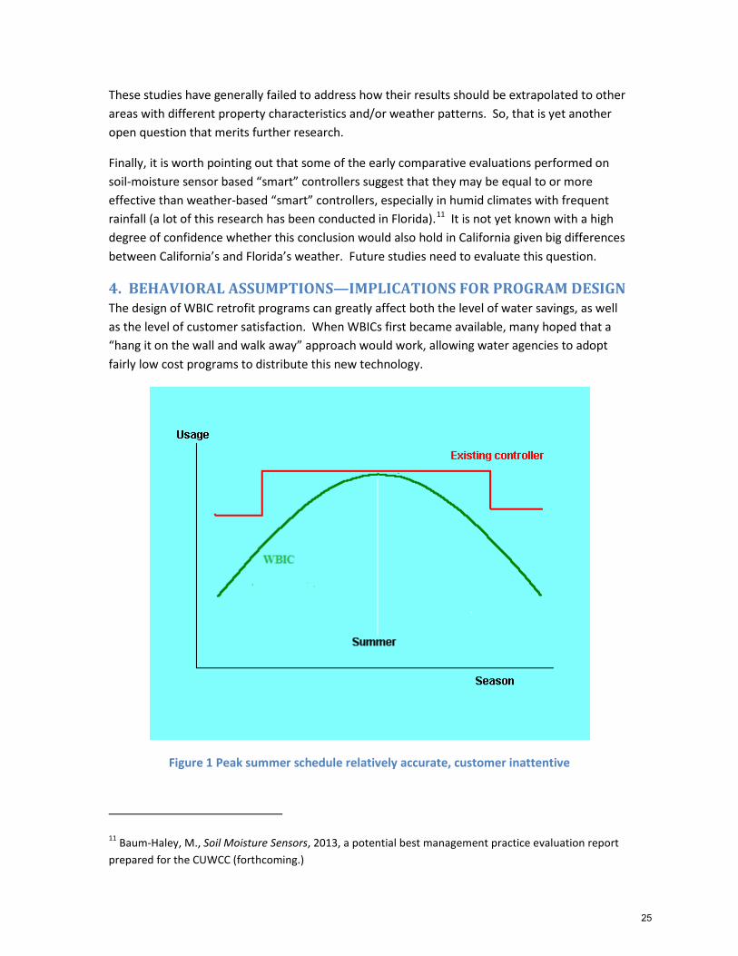
4. BEHAVIORAL ASSUMPTIONS—IMPLICATIONS FOR PROGRAM DESIGN The design of WBIC retrofit programs can greatly affect both the level of water savings, as well as the level of customer satisfaction. When WBICs first became available, many hoped that a “hang it on the wall and walk away” approach would work, allowing water agencies to adopt fairly low cost programs to distribute this new technology.

Figure 1 Peak summer schedule relatively accurate, customer inattentive

11 Baum-Haley, M., Soil Moisture Sensors, 2013, a potential best management practice evaluation report prepared for the CUWCC (forthcoming.)

25

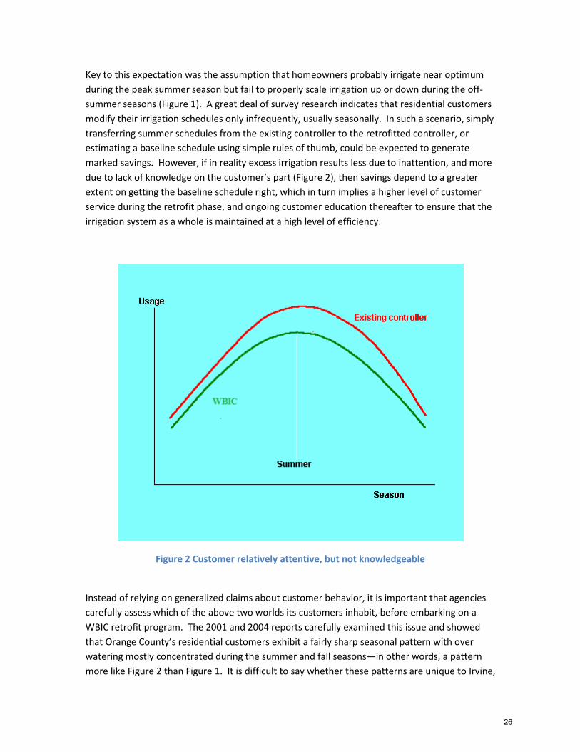
Key to this expectation was the assumption that homeowners probably irrigate near optimum during the peak summer season but fail to properly scale irrigation up or down during the off-summer seasons (Figure 1). A great deal of survey research indicates that residential customers modify their irrigation schedules only infrequently, usually seasonally. In such a scenario, simply transferring summer schedules from the existing controller to the retrofitted controller, or estimating a baseline schedule using simple rules of thumb, could be expected to generate marked savings. However, if in reality excess irrigation results less due to inattention, and more due to lack of knowledge on the customer’s part (Figure 2), then savings depend to a greater extent on getting the baseline schedule right, which in turn implies a higher level of customer service during the retrofit phase, and ongoing customer education thereafter to ensure that the irrigation system as a whole is maintained at a high level of efficiency.

Figure 2 Customer relatively attentive, but not knowledgeable

Instead of relying on generalized claims about customer behavior, it is important that agencies carefully assess which of the above two worlds its customers inhabit, before embarking on a WBIC retrofit program. The 2001 and 2004 reports carefully examined this issue and showed that Orange County’s residential customers exhibit a fairly sharp seasonal pattern with over watering mostly concentrated during the summer and fall seasons—in other words, a pattern more like Figure 2 than Figure 1. It is difficult to say whether these patterns are unique to Irvine,

26

possibly because of their budget-based rate structure, or are more general in nature (suggesting unreliability in prior survey research). That is why agencies must carefully assess this issue while designing their retrofit programs.

Expert opinion is fairly unanimous that a “set it and forget it” approach does not work well. Water conservation goals are difficult to realize until homeowners are involved in ensuring that their entire system is working properly, that is, the landscape is properly hydro-zoned, is free of leaks, has appropriate nozzle hardware with proper pressure regulation, the controller is correctly programmed, its “smart” features are actually working, and so on. This is true of both weather-based and soil-moisture based “smart” controllers. The homeowner’s involvement may range from as simple a matter as changing batteries especially if the weather or soil-moisture sensors are wireless, to a deeper understanding of horticultural and irrigation science to be able to correctly program their “smart” controller. Some of the water savings that we expect from “smart” controllers comes from correctly programming parameters such as, soil type, plant type, slope, shade, etc. Relying on default inputs can rob a “smart” controller’s ability to save water.

Finally, it must be remembered that the word “smart” does not always conjure the same meaning for homeowners as it does for irrigation professionals. Many homeowners associate the word “smart” with a controller’s ability to interface with a computer or smartphone, not necessarily with water use efficiency, which is why outreach and education are so important.

5. COSTS Estimating the cost of a new WBIC has become quite complicated given the plethora of models, manufacturers and hardware combinations that are now available to the residential consumer. At one end are add-on weather sensing modules that can be purchased and connected with an existing controller to make it “smart.” Not all controllers have the ability to accommodate an external sensor, but many do. At the other end are fully integrated units that would need to be purchased as a package to replace an existing controller. The add-on weather sensors for a 6-8 station residential controller can usually be purchased for under $100. Fully integrated “smart” controllers for residential applications can cost anywhere between $200 and $500, with a few models costing a great deal more. Professional installation can easily add another $100 to the cost of a new “smart” controller. The cost range for soil-moisture based “smart” controllers appears similar to WBICs. Given the rapid innovation that is taking place in this technological space, cost information will remain bit of a moving target requiring frequent market updates.

6. DEVICE LIFE There are no good field data for estimating the average life of a WBIC. Expert judgment by landscape professionals generally places it at roughly 10 years. While this may be a good estimate for the main controller mounted indoors or within an enclosure, the outdoor weather sensors if present may have significantly shorter lives because of their exposure to the elements. How many replace faulty sensors in a timely manner, and how many simply accept a “smart” controller that has defaulted to a traditional controller? Similarly, those that need to

27

subscribe to a paid weather data service for making their WBIC work in “smart” mode, how many cancel this service before the main controller fails? We don’t yet have good answers to these questions.

7. THE CHALLENGE AHEAD Several questions remain unanswered despite great interest in WBICs and many completed field trials. These include:

1. How should savings estimates obtained from field trials be extrapolated to other areas with very different property characteristics and/or weather patterns?

2. How should wasteful irrigators be identified and steered toward WBIC retrofit programs? What customer targeting rules lead to a cost-effective retrofit program?

3. What is the longevity of savings associated with WBIC retrofits? What actions should be taken to enhance savings longevity?

4. How do savings compare between weather-based and soil-moisture based “smart” controllers? Which circumstances favor one over the other?

With respect to the first two questions, it is important that future field evaluations build a “look forward” feature into their study design. It is not enough to estimate what a certain program saved in retrospect. It is also important to provide a way for others to assess that if program XYZ saved a certain amount of water in a given service area, how much is a similar program likely to save in another area with different socio-economic and weather characteristics. Very often, a field evaluation will report savings in terms of gallons per household or percent reduction per household without providing any sense for how these savings varied by different household characteristics, such as total water use, or lot size, or irrigated acreage, or level of wasteful irrigation prior to the retrofit. Without such granularity, however, others cannot extrapolate a study’s results to their own service areas. We hope future studies will go the extra mile to make their findings more broadly applicable, in the bargain also improving our ability to dissect and compare an evaluation’s results with those of other such evaluations.

28

DISCOUNT RATES To undertake least-cost planning, water suppliers must be able to rank future supply options in terms of their level of cost-effectiveness. But, how should one compare different supply options on an apples-to-apples basis when each is potentially associated with a different time profile of costs and water supply yields? A method devised to accomplish this is called discounting, whereby all initial and future costs and water supply yields of a supply program are expressed in terms of their present-day values. Once this is done, costs and supply yields can then be easily compared across programs. A key input required to perform the discounting is called the discount rate. Selection of an appropriate discount rate is the only topic covered here. For a full description of how to apply a discounting framework to a complex stream of costs and water supply yields spanning multiple years, please refer to other appropriate CUWCC products1.

Discount rates are meant to capture the time value of money. Individuals are willing to invest some portion of their current income only if this investment (deferred present consumption) is likely to yield greater income (greater consumption) in the future. Or to put it differently, individuals value current consumption more than future consumption. Were this not true the concept of interest would not exist. An individual willing to forgo $1 of present consumption only if promised $1.1 a year later indicates through his behavior that his nominal annual discount rate is 10%. One could turn this statement on its head and say that the present value of $1.1 obtained next year is $1 in today’s terms, which is really the key to performing cost-effectiveness analyses. The real discount rate, however, is equal to the nominal discount rate minus the rate of inflation. If we assume annual inflation is running at 5% in the above example, then asking for $1.1 next year to replace $1 of deferred consumption this year implies that really speaking the individual only wants the purchasing power of $1.05 in terms of today’s dollars to be made whole for deferring $1 of present consumption. In others words, his real discount rate is roughly 5%. When cost-effectiveness calculations are performed using cost and price data in real terms, the real discount rate must be used; and when performed using nominal cost and price data, the nominal discount rate must be used. The former practice is more common.

How should a water supplier select its discount rate? This is a vexed question with potentially many different answers. A water supply project may be funded via new bond issues. Some might argue in favor of the bond interest rate to be used as the discount rate. However, bond interest rates reflect not just the time value of money but also perceptions about the riskiness of the bond issuer relative to risks associated with competing investment alternatives. A bond backed by the full faith and credit of the US government requires a lower interest rate to sell, than that issued by the State of California, which in turn is lower than that issued by a water utility. Even if this conundrum could be easily solved, what discount rate would one select for capital improvements or conservation programs funded via water rates instead of bonds? Therefore, while bond interest rates are useful for the purpose of financial analyses, they should not be confused with the discount rate.

1 For example, the Council has developed a Cost-Effectiveness Analysis (CEA) Tool (spreadsheet and documentation) for its members that can be used to run these sorts of analyses.

29

Although the Federal government offers guidance about discount-rate selection for Federal water projects2, for the purpose of evaluating cost-effectiveness of water conservation programs, we think guidance issued by the California Department of Water Resources (DWR) is perhaps more useful3. DWR is at present using and recommending a real discount rate of 6%, “which approximates the marginal pretax rate-of-return on an average investment in the private sector in recent years.” In other words, DWR is benchmarking its discount rate to the opportunity cost of private capital, in essence expressing a preference for investments made in the water industry to be at least as attractive as investments made in private capital markets as a whole.

While the validity of DWR’s recommendation can be debated, there are three key reasons why water suppliers would do well to stay consistent with DWR’s guidance, now and in the future. First, DWR in the past has required water suppliers wishing to tap bond-financed grant funds, such as, Proposition 50 and other such funding sources to use a real discount rate of 6% in their proposals. Although DWR may revise this number in the future, it is unlikely to stop demanding consistency, crucial for maintaining an even playing field.

Second, water suppliers are no longer operating in a world where they can opt out of conservation on cost-effectiveness grounds. SB x7-7 has changed the existing paradigm, requiring water suppliers with water demand greater than 100 GPCD to lower their potable water use. Although suppliers have a great deal of leeway in how they choose to meet their future GPCD targets, the only purpose of cost-effectiveness analyses in such a paradigm is to rank-order different alternatives. Ultimately, a water supplier has to implement all alternatives from the most cost-effective to the one that just allows it to meet its GPCD target regardless of how attractive or unattractive that last option is. Rank-ordering of alternatives is generally not very sensitive to the discount rate.

Third, it makes little conceptual sense to use different discount rates, one for DWR-funded projects and another for internally funded projects. To maintain a valid apples-to-apples comparison across all evaluated alternatives it is necessary to use the same discount rate.

For all these reasons, we recommend that water suppliers stay consistent with DWR’s guidance using a 6% real discount rate for now, or until DWR modifies its guidance in the future. However, it would also be a good idea for suppliers to conduct sensitivity analyses to verify that the rank ordering of their alternatives does not materially change under lower discount rate assumptions, say, 2-3% in real terms.

2 See Economic and Environmental Principles and Guidelines for Water and Related Land Resources Implementation Studies adopted by the US Water Resources Council in 1983 and Circular A-94: Guidelines and Discount Rates for Benefit-Cost Analysis of Federal Programs first published by the President’s Office of Management and Budget in 1992, but updated periodically. 3 Department of Water Resources, Economic Analysis Guidebook, 2008.

30

SAVINGS DECAY OVER TIME

Real Decay Water savings generated by a water conservation program may decay over time either because of behavioral backsliding or because of a gradual loss in effectiveness of newly retrofitted equipment. For example, information provided through a landscape audit may initially spur participants to improve their irrigation system upkeep and scheduling, but over time some program participants may lose interest in complying with what they learned. A weather-based irrigation controller retrofit program may lose some effectiveness over time if participating property owners fail to maintain their on-site weather sensors in good working order, or if some of them quit subscribing to the weather signaling service. Showerhead retrofit programs may lose effectiveness over time if some participants replace ultra-low flow showerheads with illegally obtained high-flow showerheads, and so on. These are all examples of real savings decay. Although incorporating such information into demand forecasts or cost-effectiveness analyses is conceptually straightforward, in practice it is rarely available.

Accounting Decay In other instances, however, savings decay only has meaning in an accounting sense. Care must be exercised to ensure that the accounting methodology is appropriate for the specific questions being addressed.

Cost Effectiveness Analyses. For example, to assess cost-effectiveness of a program it is necessary to discount future costs and future water savings into present value terms so as to account for the time value of money. Conceptually, this amounts to decaying the value of future water savings, not the physical quantity of water savings generated by a conservation program. If the goal is future water supply planning instead of cost-effectiveness assessment, the quantity of future water savings should not be discounted.

Natural Turnover Models. Issues about savings decay in an accounting sense also occur while modeling the natural turnover of plumbing fixtures and appliances, such as toilets, showerheads, clothes washers, etc. Since all of these fixtures and appliances have a finite life, they eventually get replaced. Plumbing codes and appliance efficiency standards ensure that when they are replaced a significantly more efficient fixture or appliance takes the place of the old discarded equipment. Even if water suppliers implemented no equipment retrofit programs, eventually the entire stock of plumbing fixtures and appliances would become more efficient due to the existence of plumbing codes and appliance standards. Active retrofit programs only aim to accelerate what natural turnover would otherwise accomplish. Since active retrofit programs piggyback on natural turnover, water suppliers often decay savings from active programs to prevent overstating program effectiveness. We work out a case below using toilet retrofits as an example to demonstrate why this may be necessary.

Assume that the average life of a toilet is 25 years and that the probability of its replacement in any given year is constant, which works out to a natural turnover rate of 4%. Now assume 100 toilets are replaced with HETs as a result of a water supplier program in year 1. In the absence of such a program, the plumbing code would also have caused these toilets to be replaced with HETs through natural

31

turnover. The column labeled “HETs Credited to Code” shows the number of toilets credited to the plumbing code in each year even though the 100 toilets were initially retrofitted due to a water supplier program. The column labeled “HETs Credited to Water Supplier” shows the number of toilets credited to the water supplier’s replacement program in each year. Key aspects of the accounting include the following:

1. Physical water savings do not decay over time. Replacing 100 toilets this year will generate water savings from 100 toilets each year thereafter. Only the division of credit for the savings between the code and the water supplier program changes over time.

2. Credit for water savings assigned to the code increases over time while credit assigned to the water supplier decreases. This is because it is assumed that the non-efficient toilets would eventually have been replaced with HETs in the absence of a water supplier program. By the end of 10 years approximately 31 toilets would have been replaced by HETs as a result of natural replacement. Thus, plumbing codes receive credit for approximately 31 toilet replacements in year 10 for every 100 toilets retrofitted in year 1 due to water supplier programs. The residual 69 toilets remains credited to the water supplier program in year 10.

3. The credit accounting impacts the calculation of program cost-effectiveness from the perspective of the water supplier but it does not impact the calculation of physical water savings resulting from the replacement of 100 toilets.

Table 1 How 100 HETs Retrofitted by a Water Supplier in Year 1 are Allocated to Code over Time

Year HETs Credited to Code HETs Credited to Water

Supplier

1 0 100

2 4 96

3 8 92

4 12 88

~ ~ ~

10 31 69

Note that Table 1 only accounts for water savings associated with water supplier replacement programs. Total water savings from conversion of toilets to HETs is the sum of conversions realized through both natural turnover and water supplier programs. The share of total savings coming from water supplier programs versus natural turnover depends on the scale of supplier programs relative to natural replacement.

32

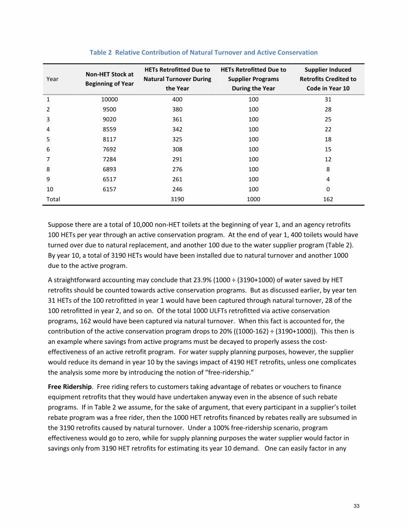
Table 2 Relative Contribution of Natural Turnover and Active Conservation

Year Non-HET Stock at Beginning of Year

HETs Retrofitted Due to Natural Turnover During

the Year

HETs Retrofitted Due to Supplier Programs

During the Year

Supplier Induced Retrofits Credited to

Code in Year 10

1 10000 400 100 31 2 9500 380 100 28 3 9020 361 100 25 4 8559 342 100 22 5 8117 325 100 18 6 7692 308 100 15 7 7284 291 100 12 8 6893 276 100 8 9 6517 261 100 4 10 6157 246 100 0 Total 3190 1000 162

Suppose there are a total of 10,000 non-HET toilets at the beginning of year 1, and an agency retrofits 100 HETs per year through an active conservation program. At the end of year 1, 400 toilets would have turned over due to natural replacement, and another 100 due to the water supplier program (Table 2). By year 10, a total of 3190 HETs would have been installed due to natural turnover and another 1000 due to the active program.

A straightforward accounting may conclude that 23.9% (1000 ÷ (3190+1000) of water saved by HET retrofits should be counted towards active conservation programs. But as discussed earlier, by year ten 31 HETs of the 100 retrofitted in year 1 would have been captured through natural turnover, 28 of the 100 retrofitted in year 2, and so on. Of the total 1000 ULFTs retrofitted via active conservation programs, 162 would have been captured via natural turnover. When this fact is accounted for, the contribution of the active conservation program drops to 20% ((1000-162) ÷ (3190+1000)). This then is an example where savings from active programs must be decayed to properly assess the cost-effectiveness of an active retrofit program. For water supply planning purposes, however, the supplier would reduce its demand in year 10 by the savings impact of 4190 HET retrofits, unless one complicates the analysis some more by introducing the notion of “free-ridership.”

Free Ridership. Free riding refers to customers taking advantage of rebates or vouchers to finance equipment retrofits that they would have undertaken anyway even in the absence of such rebate programs. If in Table 2 we assume, for the sake of argument, that every participant in a supplier’s toilet rebate program was a free rider, then the 1000 HET retrofits financed by rebates really are subsumed in the 3190 retrofits caused by natural turnover. Under a 100% free-ridership scenario, program effectiveness would go to zero, while for supply planning purposes the water supplier would factor in savings only from 3190 HET retrofits for estimating its year 10 demand. One can easily factor in any

33

assumption about free-ridership, from zero to 100% depending on the best information available4. Free ridership then is potentially yet another reason for decaying savings projected from an active conservation program.

In summary, savings decay may be a real phenomenon or it may be necessitated by the needs of proper accounting. Water conservation professionals must conceptually be clear as to why they are decaying savings, and only then select an appropriate savings estimation methodology.

4 Whitcomb, J., Free Riders in ULFT Programs, a report prepared for the California Urban Water Conservation Council, 2002.

34

NATURAL REPLACEMENT RATES Plumbing fixtures and water-using appliances have a finite life, causing them to be replaced upon failure. Sometimes the cause of replacement may be home remodels instead of equipment failure. This distinction is probably not very important if the main focus is quantification of the total natural replacement rate, although the underlying driver of natural replacement may have some bearing on program “free-ridership” rates. On the other hand, what is undoubtedly important is the existence of plumbing codes and appliance standards, which ensure that old equipment is replaced with new water-efficient fixtures and appliances. This natural replacement dynamic must be properly understood before the impact of active water conservation programs can be reliably quantified.

In all likelihood, the risk of equipment replacement due to failure or home remodels is not constant over the lifetime of a piece of equipment, be it a plumbing fixture or appliance. In general, failure risk is low during the early years, rising thereafter as components fail but are repaired or replaced without the whole unit being discarded, until it finally is.

For most common plumbing fixtures, such as toilets and showerheads, or appliances like clothes washers, these risk profiles as a function of age remain poorly documented. And even if these risk profiles were better known, another piece of information would also be necessary before anything useful could be done with these risk profiles—one would need to know the distribution of age in the stock of fixtures and appliances that exist in a water supplier’s service area. This second piece of information is also hard to come by. Therefore, water conservation professionals are forced to assume that the risk of equipment replacement, due to home remodels or failure, is constant over the life of the equipment. Water conservation professionals have generally assumed that the average life of toilets, showerheads and clothes washers is roughly, 10, 25, and 14 years, respectively—implying annual turnover rates of 10%, 4%, and 7.1% under the assumption of constant replacement risk over the life of the equipment.5 How reasonable are these assumptions?

To address this question we have compiled data from previously completed household surveys (Table 3). Since these were completed at different points in time they can shed light on whether our natural turnover assumptions are compatible with what we see as the increase in saturation of efficient equipment over time.

5 An average life of 10 years for showerheads implies a natural turnover rate of 10% per year (that is, 10% of a given stock is replaced in the first year, 10% of the remaining stock in the second year, and so on). In other words, 10% of a given stock has a life of 1 year, 9% a life of 2 years, 8.1% a life of 3 years, and so on. Roughly 35% of the initial stock would have a life exceeding 10 years. The average of this distribution of lives works out to 10 years. Mathematically speaking, if x0 is the number of inefficient devices at the start of the analysis, and the natural replacement rate is denoted as r, then the number of inefficient devices remaining in year t>0, xt, is given by

xt = x0 1− r( )t

The number of installed efficient devices in year t>0, yt, is given by

yt = x0 1− 1− r( )t[ ]

35

Table 3 Results from Prior Saturation Studies

Single Family Saturation Multi Family Saturation

Study Location6 Survey

Year

LF Shower-

heads ULFTs or

HETs HE Clothes Washers

LF Shower-heads

ULFTs or HETs

HE Clothes Washers

EBMUD 2001 67% 34% 12% 64% 37% 7% Orange County 2000 67% 49%

60% 38%

Santa Clara 2002 59% 42% 26% 51% 31% 29% Santa Cruz 2012 92% 90% 63% 95% 89% 58%

From the saturation rates in Table 3, one can calculate an implied turnover rate that is really the sum of both natural turnover and the turnover caused by active programs, or in the case of Santa Cruz, its retrofit-upon-resale ordinance applicable to toilets and showerheads. The effect of Santa Cruz’s retrofit-upon-resale ordinance in boosting the saturation of efficient toilets and showerheads looks quite remarkable. These implied turnover rates are shown in Table 4, calculated assuming that only ultra-low-flush toilets and low-flow showerheads were available in the market since early 1994, and that high-efficiency clothes washers became widely available only around the beginning of 2001. For the sake of these calculations, we assume that saturation rates shown in Table 3 reflect conditions at the end of the survey year.

Table 4 Implied Turnover Rates from Prior Saturation Studies

Single Family Saturation Multi Family Saturation

Study Location Survey

Year

LF Shower-

heads ULFTs or

HETs HE Clothes Washers

LF Shower-heads

ULFTs or HETs

HE Clothes Washers

EBMUD 2001 12.9% 5.1% 12.0% 12.0% 5.6% 7.0%

Orange County 2000 14.6% 9.2%

12.3% 6.6% Santa Clara 2002 9.4% 5.9% 14.0% 7.6% 4.0% 15.7%

Santa Cruz 2012 12.4% 11.4% 8.0% 14.6% 11.0% 7.0%

The lowest implied turnover rate for toilets, showerheads and clothes washers (shaded green in Table 4) then becomes our best estimate of the “natural” turnover rate under the assumption that the others are higher because of the effect of active conservation programs or ordinances. Admittedly, even the 6 These data have been obtained from the following studies: Water Resources Engineering, Inc., Water Conservation Market Penetration Study, a report prepared for the East Bay Municipal Utility District, 2002. Metropolitan Water District of Southern California and Municipal Water District of Orange County, Orange County Saturation Survey, 2002. M. Cubed, et al., Santa Clara County Residential Water Use Baseline Survey, a report prepared for the Santa Clara Valley Water District, 2004. Envirosmart Solutions Group and Western Policy Research, Residential and Commercial Baseline Water Use Survey, a report prepared for the City of Santa Cruz Water Department, 2013

36

lowest estimates may have some active-program effects buried in them. One would need detailed data about past conservation programs to separate those effects out. But, overall, Table 4 suggests that assumptions about natural turnover that water conservationists have made in the past appear to be reasonable.

37