bnl mad harmonic analysis based orbit correction … notes/tn456.pdf · minimizes the least squares...

For Internal Distribution Only

Accelerator Division Alternating Gradient Synchrotron Department

BROOKHAVEN NATIONAL LABORATORY Upton, New York 11973

Accelerator Division Technical Note

AGS/AD/Tech. Note No. 456

BNL MAD

Harmonic Analysis Based Orbit Correction Commands

AGS Booster Applications

J. Niederer

February 24, 1997

BNL MAD

Harmonic Analysis Based Orbit Correction Commands

AGS Booster Applications

J . Niederer

AGS Department Brookhaven National Laboratory

February 24,1997

1. Introduction A method of using charged particle orbit data to compute coefficients of a Fourier series for sets of

orbit corrections is described. An accelerator lattice is defined as well as practical with what is known about machine conditions. Any remaining differences, monitor errors, and other unknowns are then lumped together and approximated via a harmonic series applied to a family of calibration correctors. This family can be real correctors for convenience, or virtual ones distributed throughout the lattice for calibration / correction purposes only. This method has been added to the local BNL MAD programming environment, and demonstrated with such elderly AGS Booster data as available.

Various kinds of harmonic based orbit correction schemes have been practiced on most accelerators now for years. What may be a little different here is using such a scheme to bring accelerator models into essential agreement with actual measurements, thus providing an absolute basis for guiding orbit controls. Furthermore, the algorithms to be described appear to be extremely stable computationally, and hence very suitable for automatic orbit control application. The scheme can tolerate individual components popping in and out of service, and a fair amount of the other disorder that often accompanies actual machine operation.

In the calibration mode, orbit measurements are used to adjust a set of conventionally arranged correction elements (real or virtual) to match the measurements. A closed orbit is computed for each of a set of trial amplitudes for a harmonic pattern on the calibration correctors to search for an amplitude that minimizes the least squares residuals between the orbits by computation and by snapshot. The result is a set of harmonic amplitudes, and a %est fit" momentum offset term delta P for the X plane, and an a0 term for the Y plane. Harmonics are subtracted off one at a time, and are relatively insensitive to the order of subtraction, and to gaps in the recorder and corrector patterns. In the AGS Booster application noted here, all fitted amplitudes are well behaved, being well under the maximum orbit excursions. The expected J = 4 and J = 5 contributions are larger, and the others are smaller, and presumably help to measure the noise level of the method. One can watch the reduction of the least squares progress as each harmonic is fitted. This procedure effectively calibrates the program, using the smoothing properties of the harmonic approxi- mation and the lattice optics to adjust the program as needed to yield the measured orbit. The program with the fitted adjustments is now able to reproduce the measurements within some quite acceptable margin of error. The resulting configuration typically reduces the discrepancies between the calibration measurement set and the closed orbit found by the program by a factor of ten or better.

In a second step, the now calibrated program may be asked to alter the orbit from the original measurements to something else, such as a flatter orbit. Orbits are now computed for trial harmonic patterns on the real correctors, and a penalty function comparing the desired with the measured orbit is minimized. The change in the real correctors is now in principle an absolute set of numbers, as the program has been calibrated to match the starting orbit values. The procedures are readily iterated to reduce further any

remaining discrepancies. The notes describe the somewhat experimental MAD command setups, the graphics capabilities, and

some demonstration results. A new command, Vcorrs, gathers the necessary information and performs the computations. The emphasis here is to report the apparent possibilities of the method rather than provide polished code and a manual. The method is a rather straightforward extension of the constrained amplitude subtraction procedure described previously, and implemented in the Vharm vector harmonic analysis command. In their current state of development, the commands and data needed are probably more complicated than they really have to be, and if any interest is aroused, may be expected to improve.

These notes use the language of orbit positions, and orbit monitors and correctors, in the conven- tional sense of the usual MAD lattice element definitions. Procedures are based on the notion of families of similar monitors and correctors, identified by names in lists. Actually the program can work with any family of distributed magnets, windings, or fudges with common attributes. Similarly it can provide fits to other practical kinds of distributed measurements as well.

2. Constrained Fits Experience with the Vharm vector harmonic analysis command of the local BNL version of the

MAD accelerator program indicated that constrained amplitude subtraction of individual harmonics produced reasonable results that were rather insensitive to missing items or regions of the sampled data set. The fitted functions behaved properly between the fitted data points, as well as at the points themselves. Input values could be be irregularly spaced: spacing was not restricted.

In the familiar problem, a pattern of I measurements Vi taken at locations Si over a distance Smax is to be fitted to a harmonic series:

j=jniax j=jmax

j=jniin j=jmin V i=Ao+ Ajcos (2n jS i /Sm, )+ Bjsin(2n:jSi /Sm,)

When treated as an extremal problem, the set of Aj, Bj are found by minimizing the difference at each point between the measurement and the fitted function. The measurements may also be weighted individu- ally, with weights noted by Wi. The function to be minimized is:

i=I j=jmax j=jmar

i=l j=jmin j=jniiii zwi (vi - A ~ - COS (2 n: j si / sm,) - B~ sin (2 n: j si / s,,))*

This general form of the fitting criteria is adjusted somewhat for the realities of working with corrector sets. In the present application, the intent is to place an optimal harmonic pattern on a family of correctors, rather than merely analyze orbit measurements in terms of harmonics. The function to be minimized now becomes:

i=I

i=l xwi (Vi - Tj>2

where the Ti are computed values at the monitors, obtained from closed orbit tracking computations. The trial amplitudes Aj and Bj are considered in the orbit measurement space of the monitors, and constrained to be within some fraction of the largest measured amplitudes. These trial values translate to the family of corrector values as:

j=jmax

j=jmin C i = F i ( Fcorrj(Aj cos(2njSi/Sm,) + B j s i n ( 2 n j S i / S , , ) ) )

where the Si' are now the corrector locations along the orbit. The individual factors Fi for the correctors are applied as given, and the common Fcorr factors computed from the changes in all of the Ti produced by an incremental harmonic change dCi in all of the correctors. Fcorr is somewhat artificial, and is intro- duced only to help with the amplitude constraint, which is expressed in terms of the orbit measurements. These factors are a measure of the efficiency with which a given harmonic is produced in the orbit when placed on the correctors. The practical range of actual corrector values is limited as well. While the program offers an optional feature to clamp corrector values, the values achieved so far have been sufficiently reasonable that further constraints have not been considered,

T

7 - 3 -

In a textbook styled implementation, corrector and monitor sets have similar placements and periodi- cities, and perhaps the two kinds of analysis may then be essentially equivalent, but such regularities are not a precondition here. Except for institutions where there is some deep seated religious aversion to working monitors and correctors, the scheme should be adequate for any reasonable configuration of monitors and correctors.

In the calibration mode, the model is asked to modify itself in terms of harmonic based corrections to satisfy given orbit measurements (snap shots). In the X plane the fixed A0 term represents an average displacement, which physically is a result of a momentum offset from the so called reference orbit, so this offset delta P is adjusted in the model to match the snap shot data. This adjustment should cause the A0 term to vanish. It provides a smooth adjustment to the model at every element of the orbit, which is prefer- able to a set of kicks at sparsely located correctors.

After the momentum offset has been obtained, the constrained method selects for each harmonic j an even (A) and odd (B) coefficient that produce the largest reduction of the above penalty function. Initially, the weighted squares of the difference between each point of the data set and the computed contribution from harmonic Aj, Bj are summed to obtain the penalty. The program searches in an Aj, Bj space for this reduction. The Aj and Bj pairs must satisfy the relation

A; f B? < Constraint * Initial-Amplitude2

Trial sets of Aj and Bj amplitude pairs are cycled, over a grid that is reduced over succeeding passes. First an Aj is cycled over a few intervals of day where da is formed from the largest residual amplitude as:

0

da = dconstraint * Abs (Rmm) I Ndivs

Ndivs is some specified number of divisions, perhaps about 8 or 10, which balances accuracy against minimizing the number of rather slow orbit computation passes. In the first pass, both Aj and Bj are taken as zero. A crude search is made by computing penalty functions of residuals, starting with the initial value for Aj. A minimum point and its two neighbors are sought. These three points are interpolated quadrati- cally to estimate a minimum. Using this estimate for Aj, the steps are repeated for the corresponding Bj over a range subject to the constraint. The interval da is reduced about the best Aj, the penalty calculations repeated using the now best Bj, and Aj further localized. Then Bj is similarly cycled in steps of smaller db using the best Aj. The steps are repeated a few times, as needed to converge. The contribution of this Aj and Bj is added to the accumulating values on the correctors. The process is repeated for the next, and remaining harmonics. If iterated further, the starting Aj and Bj are taken from the previous best values, and any further changes to the Aj and Bj are sought over a reduced search region with a smaller constraint. When finished, the Vi - Ti residuals are a measure of the fit over the given range of harmonics. The sum of the squares of the residuals, the penalty function, is now in a sense a least squares for the fit.

As with the Vharm procedure, several options are provided to help test the validity of the fits. In a Pernzute option, the order of processing of the harmonics can be scrambled. The fits of a set of harmonics are repeated in a pattern which begins with a pivot harmonic, jmain, followed by the next lower one, then by the next higher one, until the range has been covered. The pivot is then advanced by one, and the next version of the pattern repeated. For low order harmonics, the method has appeared insensitive to the order in which harmonic contributions are subtracted. There are some minor differences among these trials with permuted orders, but they appear well within expected errors, and tend to involve harmonics which have little overall effect. In the Drop Mode option, the fits can be cycled over a pattern which drops one of the data points, performs the fit, restores the dropped point, and repeats with the next point dropped. A dropped data point that leads to a markedly better fit may cast some doubt on the point. Results may have some minor sensitivity to the dropped point in the overall orbit averaging, but for the most part they do not have the wild swings often produced by other methods.

The constrained subtraction method is somewhat slow because of the relatively large amount of searching and attendant closed orbit calculations, especially if the permute or drop mode options are used. For reasonable search patterns, and with debugging code, a 24 point Booster data set and orbit takes about 9 seconds per harmonic on a loomips workstation. From about 15 to 25 closed orbit passes are involved, which is perhaps a little larger than needed once convergence is established. For someone in more of a hurry, most of the closed orbit passes can be done in parallel on a suitable parallel computer.

4 -

3. Results This procedure works rather well for the rather small and regular Booster lattice. It is not yet at all

clear how general it may be, as it needs a lattice understood well enough to yield a closed orbit when modeled. The example calculations have not yet been exercized with markedly non linear conditions. It can probably be argued that both the choice of machine and of the data sample used to develop the codes plays to the particular strength of the method. One or two bad data points cause the phases of the various harmonics to line up to satisfy the excursions at these points, which dominate the penalty function. Simi- larly where the phases are out of alignment, the orbits are better behaved. Yet when offending points are removed, the phases of the principal harmonics remain about the same. For the rather dirty Booster orbits considered here, there is always a clean minimum in both Aj and Bj as the cycling is carried out. The results do not cluster about the end points of the constrained ranges of A or B, as if a preferred result were outside of the range. The order in which the Aj, Bj are evaluated and subtracted off does not seem to matter. When apparent bad points are skipped, the scheme produces even smoother results. The scheme is insensitive to missing points, and so far has not encountered the artifacts of the usual Fourier analyses when data is missing and patterns are broken. The resulting corrector patterns are balanced, and the changes have little effect on tunes. More elaborate trials with a wider range of data and afflictions are clearly needed, but these preliminary results are rather encouraging.

Several representative screen plots obtained by analyzing data from an AGS Booster orbit snapshot are shown in Figures 1 - 5. These examples are intended to illustrate the methods rather than to offer con- clusions from the data sampled. This particular data, from an off momentum orbit of 1993, was obtained to test the extraction of the proper momentum from orbit data back when these things still worked. It is quite likely that something in the C8 region is turned on and didn’t make it into the model, or maybe the data point itself is off by a centimeter or so. The Pvcorrs drawing command displays amplitudes and phases of individual harmonics, and the buildup in the form of curves of sums of harmonics Jmin --> N, as N is increased from Jmin through Jmax. Monitors are missing at D6 and F6, and the point from monitor C8 is rather obviously suspect, which further strains the resolving power. Calibration studies using the dropped point mode also cast doubt on the A2 data point. Correlated distortions do appear to suggest a noticeable second and third harmonic in this particular set of readings. Spurious harmonics are weaker in similar curves run without the C8 entry, but such efforts to clean up the data are not considered further here. The seventh harmonic, perhaps an artifact of the fitting, is often a useful measure of the resolution and noise in the method. The apparent J = 7 amplitude here is spurious, because it has little effect on the fit, and because the spacing of the correctors limits the efficiency with which it is expressed.

The Figures present the results of an exercise which calibrates the model in terms of a specific snapshot taken at a momentum offset of about - .0015, and moves the orbit from the snapshot values to a centered flat one, operating in the X plane. In Figures 1, and 2, all points of the sample are used, including the dubious A2 and C8 ones. In Figure 3, calculations similar to those of Figure 2 with these two points removed is shown. The program doesn’t seem to mind the difference. These results are for a single iteration. A second fitting pass removes completely the remaining trace of the mainly fifth harmonic.

In these Booster data samples, the harmonic analysis averages rather broadly as the orbit is measured at essentially regular intervals, rather widely spaced with respect to dimensions of likely sources of orbit distortions. But as noted before, in one sense the Booster is perhaps an extreme case in that the number and spacing of monitors barely covers the range of orbit harmonics present in the machine. Details of finer structure are obviously limited by the number of sampling points. (Figure 1) A few X plane monitors between these intervals, perhaps by adding an X coordinate to several of the Y plane monitors, would be very helpful.

A subset of statements copied from a larger test file which applies the harmonics commands dis- cussed here is appended, and described in Section 4 below. The Figures are generated from these inputs as well. Parts of the resulting PRINT file of the Vcorrs fits to this sample data are also included, and described in Section 5.

T - 5 -

4. Command File for Vcorrs A partial set of Vcorrs and related commands from a library file of MAD input statements is dis-

cussed in this section. This information, together with a plot description file, should be adequate for running the corrector based features of this part of the program. While complicated, as a library of useful commands the file is readily edited for new applications. This style permits tailoring of conditions and graphics from input statements, rather than hard coding the morass of details about tuning computations and what is to be drawn. The various array names used here are generally enclosed in quotes, making them upper / lower case sensitive, to avoid accidental conflicts with lattice element names. This example fits the calibration to 20 Booster .orbit data points of the 22 Bpms available, dropping the points at A2 and C8. A data point is dropped by setting its corresponding weight to zero. (Wgts-CZO array) The program reads the listed commands in store mode, that is it parses and stores them in the data base, but does not execute them until called to do so after the library has been assembled. Drawing commands for each case are included in the picture list, and calIed from menus by the T.pZx Plcalls screen manager command. Details of the Vcorrs fitting and Pvcorrs drawing commands are given in later sections.

8

4.1. Calibration Command Group The example Vcorrs command here works with lists of the actual 24 bpm and 24 corrector names,

and corresponding weight and factors arrays defined as MAD Vectors. Both arrays are given the same typical values for all valid elements. These values are the same as the program defaults. For convenience, our calibration corrector set is taken to be the actual Booster corrector set. Alternatively, a finer grained virtual corrector set with zero lengths could have been defined and inserted in the latdce description.

As this part discusses a calibration run, orbit measurement data in an array called X-Data is needed, and so the array is listed here. Bpms are missing for the D6 and F6 positions, but entries are filled in anyhow by the controls operation that records orbit displacements, a convenience to preserve the general symmetry of the lattice naming conventions. The two false entries are marked by large values, which are rejected by the Filter = 999. feature. This data is in millimeters, and so the Convert = .001 feature is applied to get the data into meters. The names of the attributes of the quantities to be read from the bpms and to be set in the correctors are given as Bparams = IX and Cparams = IDpx; these could be omitted as they are the same as the defaults. These particular attributes are specialized cells of BNL "Fast" version monitors and correctors that can be read or set dynamically while the program is doing tracking. A range of harmonics from 1 through 9 are to be fitted. The total length of the orbit Smux is given, along with typical Cycles values for number of iterations, number of steps in searching for minima, and number of passes over decreasing search regions.

Also included in the group is an Ftwiss command to initialize and perform closed orbit calculations for the fitting, and commands to save, archive, and retrieve fitted corrector and momentum offset results needed by later activities. When applied to the lattice elements involved in a closed orbit calculation, these results should reproduce the original measurements to within some error. The presumption is that someone will review the calibration results, and perhaps even repeat them with dubious data points removed, before applying them. As a calibration in principle can be used for a number of further correction adjustments, calibration results are preserved separately. In this example, the perhaps cumbersome notation for commands and saved vectors and files applies the suffix C20 to note a calibration using 20 data points.

The CaZ20 subroutine group combines these stored commands to carry out the calibration, and saves results as files suitable for running in the actual correction mode. The detailed printing from FTwiss should be shut off, as closed orbit tracking passes will be made at the beginning and ending of the fitting to monitor tune shifts.

4.2. Correction Command Group The run mode finds the changes needed to move the orbit from the one calibrated in the model to

some other one, given as recorder values held in the Goodorbit vector. In this example the goal is a flat orbit with all values 0. at the bpms. Actual bpm data are not needed for this move. The lattice calibration corrector family and momentum offset are set initially to the calibration values, using Retrieve and VtoD (Vector to lattice family Data) commands defined in the groups. The momentum offset value from the calibration is largely useful for an initial FTwiss pass that reproduces previous conditions. The offset most 0

b

< - 6 -

likely will be changed as the orbit is moved to the desired one. Data conversion and filtering is generally not needed for the Vcorrs command in the run mode,

unless actual data for the intended orbit warrants them. Results to be saved optionally for later screen plotting are noted: the table of coefficients Brun-R20, and the momentum offset P-savR20. The coefficients of the pattern on the correctors are also in the table.

The Run20 subroutine group combines these library entries, and produces a listing of the corrector and momentum offset changes that yield the given orbit changes. It also saves these results as archived files, suitable for input into the drawing commands.

4.3. Drawing Commands The Pvcorrs drawing command draws curves from the coefficients computed during the fitting,

stored in a table, and saved for displays. As the fitting is usually slow, the drawing is done separately from the preparation of the table. The same command can draw both individual amplitude and synthesis curves. Each refers to a Vcorrs command to find the table, and organize the arrays and other features needed by the original fitting command to prepare the table. These operations need the coefficients table Brun-RZO, and the fitted factors F-savR20 which relate the effect of correctors changes to orbit displacements. The table carries the fitted momentum offset. The operations further depend upon the FW-Drw Ftwiss command keyed to the DrawC6 PldrawR vector drawing command. The vector drawing command works within an Ftwiss run, accepting an array of orbit variables after each lattice element. Entries in the plotter description file are keyed to these variables, through the Cdef6 Curvedef command and its descriptive arrays, which handle selection of variables, colors, line types, and plotting factors and offsets.

At the very end, the T.pk Plcalls screen plotting manager is called to cany out the plotting via various menus and elaborate description arrays from a separate plot command library file not considered further here.

5. Vcorrs Outputs Sample outputs are given using the commands noted above, for both calibration and correction runs.

The two corrector families need not be the same for calibration and correction runs, although they are here. This extravagance with paper is mostly to give the reader a proper feel for the stability of the method. All data points are included in these results. Listings begin and end with a Twiss run to show closed orbit sum- maries for starting and fitted orbits.

A short table gives the progress of the fits as the several harmonics reduce the least square penalties. As the computations involve a number of closed orbit calculations which can be slow, this table is also printed on line to give some hint that the program is doing something. The table gives the fitted amplitudes relative to the bpm data, the current penalty, clock time, the reduction of penalty due to the current harmonic, and the number of closed orbit passes needed to reach a tolerance. The progression rather dramati- cally picks out the relevant harmonics, and sizes are bounded for the harmonics which are expected to be small, or noise.

Next a Fit Summary Table lists the fits to the measurements in the case of calibrations, or to the requested orbit in the case of applying corrections. The V Initial column gives the Twiss computed values from the uncalibrated program in the case of a calibration run, or the computed values from the calibrated model before adjusting to the requested orbit. The Adjusted columns are intended to measure any left over offsets after the harmonics have been fitted, perhaps a measure of noise, or asymmetric bpm data sampling.

The Correctors Sunzmary Table has columns giving the final corrector values, the initial ones, and the differences, presented as angular kicks in radians. The Change column is an absolute adjustment to the real correctors computed by the fitting.

6. The Vcorrs Command Like its predecessor Vharm, the Vcorrs command analyzes data arrays expressed as MAD Vectors.

Vectors are identified by name in the inputs. Several options describe the range of sampling and outputs. In the Permute mode the fits are repeated with different sequences for the subtraction of the several harmonic contributions. In the Drop mode the fits are repeated in a sequence which drops one input point at

- I -

each step. The drop feature offers a way to examine potentially bad monitors, aid in data selection, and explore sensitivity of fits to particular monitors. Data selection can be obtained dynamically with the filter option and selective weighting.

The command accepts sets of measurements or program output expressed in vector format, at given named lattice monitors at locations S , with optional weights. The calibration mode expects one or two data sets, nominally X and Y orbit displacement values at their respective sampled locations. If wanted, data from both dimensions can be treated by one command. A range of harmonics consistent with the number of data points may be selected. In the X plane, instead of the fixed term, the momentum offset is always computed, and the program adjusted accordingly. The fits can be iterated to remove the biasing effect of ostensibly missing data upon the fixed term, if experience suggests that this effect is significant. In successive iterations, missing data points are computed from the fitted results of previous iterations. Output is to printed tables of inputs and fits, and optionally to an internal harmonic table which can be directed to harmonics synthesis plots, and individual harmonics plots.

In the following, the attributes are grouped into categories of name lists and vector arrays, program options, harmonic selections, and output options. The essential information includes the names of the lists holding names of the monitor and corrector families, and measurement data. Names are still limited to eight characters, and monitors and correctors must be uniquely named. Emplacements of both monitors and correctors are taken from the lattice used for the orbit computations, and so are not needed as inputs. Most other quantities have defaults adequate to get the calculations started. Some of these details will change with further experience.

As the families of bpms and correctors can differ for calibration and correction runs, separate data groups may be involved. Normally both groups work off the same lattice description, which can be quite littered with parameter expressions, some of which are likely to depend on the momentum offset. Hence the passing of calibration results to later runs can involve considerable complication in lining up the various parameters. There is a further possible confusion in that correctors are reset from the user supplied KICK attribute at the beginning of a closed orbit pass, but operate from the derived internal lDpx and lDpy attributes once initialized.

6.1. Input Data Vectors

Bpms(2) The Nume(s) of simple list(s) of data point label names, X and / or Y. ( List, Menu, or Xmenu form) Normally these are names of members of a family of monitors, but any family of similar elements that yield a common kind of measurement may be submitted. These names are also used to label entries in least squares fit tables. Null entries may be included to maintain systematics and habits of listing. All monitor related arrays, such as measurements, weights, and good orbit values, must have the same length and indexing as this defining Bprns list. The Nume(s) of simple array@) of measurements, for example, a set of bpm readings, needed to define the calibration standard in the calibration mode only. X or Y (or both) must be given, and the number of entries in the vector(s) must agree with that of the Bpms list. The array of decimal values is defined as a MAD Vector. Units should be in meters, but conversion to meters can be arranged with the use of the Convert attribute noted below. Erratic input values can be rejected by the use of the Filter attribute noted below. In an automatic orbit controller application, each logical bpm would normally be connected to a practical filter, such as a MAD filter neuron. The differences between the current filtered signals and the calibration values amount to error signals, that inspire a response as computed by the Vcorrs acting as a controller.

Goodorbit(2) The Nurne(s) of simple array(s) of decimal values, for example, a set of readings to be achieved at the bpms, needed to define the desired orbit in the run mode only. (MAD Vector form). The default is a flat orbit with 0. displacement. The number of entries in the vector(s) must agree with that of the Bpms list.

Bpmdata(2)

<

\

Weights(2)

Corrs(2)

Corrdata(2)

CoMnax(2)

Factors(2)

Csaves(2)

Psaves(2)

- 8 -

The Nume(s) of simple decimal array(s) of weights. (MAD Vector form). Optional. If individual weights are used, each weight should be the inverse square of the nomi- nal mean error for the measurement, typically .001m. Printing formats are centered about assumed residuals of the order of .001m, and least squares near unity. The default of 1,000,000. will be provided for weights if no weight vectors are given. Set- ting a weight to zero is a way to remove a data point from the calculations. This is probably more important in calibration than running, as there is little point in blanking out a value when prescribing a good orbit. The Name(s) of simple list(s) of corrector names, X and I or Y. ( List, Menu, or Xmenu form) Normally these are names of members of the family of correctors, but any family of similar elements that yield a common kind of orbit change may be submitted. These corrector names are also used to label entries in least squares fit tables. Null entries may be included to maintain systematics and habits of listing. All related corrector arrays, such as factors and saved result values, must have the same length and indexing as this defining Cows list.

6.2. Necessary Attribute Smax A REQUIRED decimal number, given in meters. This is the total length over which

the input measurement set has been sampled. Smux defines the full period over which harmonics are to be fitted. It is the length of a circular orbit when a set of bpm values is analyzed. Phases for each harmonic J at corrector positions S(i) are computed as:

Theta U,i) = 2. * n * J * S ( i ) I Smux

The Nume(s) of simple array(s) of settings, for example, a set of corrector kicks in radians. When the same correctors are used for calibration and correction, these data would be the calibration values for the actual corrector set, applied for running or drawing. Optional. (MAD Vector form.) The Nume(s) of a simple array(s) of maximum permitted settings, to match the Cow- datu variables, units, and formats. Optional. (MAD Vector form.) May be helpful as a diagnostic. The fitting method inherently leads to rather small, balanced corrector values. The Nume(s) of simple decimal array(s) of factors. (MAD Vector form). Optional. Factors are used internally to translate coefficients based on orbit measurements into corrector settings. While the program will compute its own average factor for this translation from the data it is given, the use of individual factors allows for variation in response among the individual correctors. A value of 0. shuts off a corrector. The default is 1. The Nume(s) of simple decimal array(s) to receive the values of the family of correctors determined by the command. (MAD Vector form) Optional, and normally just used for calibration outputs. The saved array(s) can be initial configuration input for the run mode of fitting, by means of the Corrdutu attribute. Alternatively they can be loaded by a VtoD command into the lattice previously assembled by a USE command. The program will generate a new save vector if a named one does not yet exist. No defaults. If run in an on line analysis mode, with the calibration configured with virtual correctors, Csuves contains the actual corrector values needed to maintain the prescribed orbit, and presumably would be fed back to the control system. The Nume(s) of simple parameter command(s) to receive the values of the fitted momentum offset Delta P. Optional. The fitted offset is also placed in the preamble part of the coefficient table. In the run mode, saving and archiving these offsets can be helpful for passing fitted results for plotting. The program will generate a new parameter module if a named one does not yet exist. No defaults.

- 9 -

6.3. Attributes with Defaults Bparams(2)

Cparams(2)

Twiss

Constraint

Dropmode

Permute

Calibrate

Filter

Cycles(3)

The Name(s) of the attribute common to each member of the bpm or similar family from which the program is to obtain computed orbit data. Defaults are /X and lY for bpms. Bpms are defined as MAD Monitor, Hmonitor, or Vmonitor elements. The /X and lY attributes are specialized monitor cells that record orbit information during each pass of a tracking program. Internal names are often in quotes prefixed by a slash character to be case sensitive, and to avoid name conflicts. The Name(s) of the attribute@) common to each member of the X and / or Y correctors or similar family into which the program is to place computed settings. Defaults are lDpx and lDpy for Correctors. Correctors as used here are defined as the MAD Hkick or Vkick elements. In the BNL version the lDpx and lDpy attributes of these elements can be set dynamically by processes running within the program, such as orbit correction and feedback schemes. Note: the user supplied KZCK attribute for correctors only initializes lDpx and lDpy, but is not further involved in any changes during tracking runs. The Name of a BNL FTwiss command to be employed for the model calculations. The default will do, unless initial orbit conditions are to be prescribed. A decimal number which constrains the choice of Aj and Bj coefficients of each trial according to

A; + B; < Constraint * Znitial-Amplitude2

Ideally the value should be about l., and the supplied default is 1.2. In these studies, the constraint is seldom tripped, and then only for background harmonics that the correctors are rather ineffective in expressing. The search routines give a fairly detailed diagnostic if an apparent penalty minimum lies outside of the constraint, sug- gesting adjustment. Logical Flag: If True, the fitting will be iterated, dropping a different input reading on each successive pass. Output is not stacked, so the Htable holds only the last computation. These Drop and Permute options are useful for breaking in the program to a new problem or configuration, to establish sensitivity and confidence levels, and to identify questionable data points during calibrations. They are both rather time con- suming for routine use. Computation time increases as the number of points in the measurement sample. Logical Flag: If True, the fitting will permute the order of cycling harmonics. Com- putation time increases as the number of harmonics in the sample. Logical Flag: If True, the program will operate in calibration mode. Otherwise, in run mode. A decimal number which should be used to screen accelerator produced data such as monitor readings. Measurements greater than the absolute value of Filter will be rejected for fitting. Takes same units as, and applied only to Bpmdata and Goodorbit input arrays. 1. An integer giving the number of iteration cycles, which tend to adjust the fixed delta P result, and may influence others. Useful in reducing a harmonic that persists after a previous iteration. Successive iterations may shake up the fitting, producing more attractive fits, which may, however, differ little in final least squares criteria from others. The proper value should be obtained by trial, viewing the listing which traces the penalty function, hopefully to some convergence. The default is set for 1, to restrict inadvertent long runs, but is probably too small for most cases. The method computes a fit once without the missing points, and subsequently includes values derived from the previously fitted function at the missing points to compute the next iteration. For the AGS Booster, the contributions to the offset from the two

- 10-

missing monitors out of 24 tend to balance each other. 2. An integer giving the number of steps into which the span between the upper and lower constrained amplitudes is to be divided. Default is 8. The method of search favors about this number of steps, as searching moves in the direction of lower penalty results until an increase is obtained. 3. An integer giving the number of internal cycling passes used in searching the local grid for the best Aj, Bj pairs. Default is 5, which has proved adequate for Booster work. The program stops cycling earlier if the relative least squares improvement between cycles is less than .001, which is usually smaller than the data warrants. Each extra pass takes at least six closed orbit calculations, so there is some incentive to keep this attribute small. An optional decimal number, that if present, is used as a conversion factor for all Bpmdutu and Goodorbit input array values, and the optional Filter attribute. (Orbit measurement data)

Convert

6.4. Harmonic Selection Options

and the momentum offset fitted instead. A0 is not included in the following J ranges. Harmonics are indexed here by the letter J. In the X plane, the lead term, J = 0, (AO), is treated as 0,

Jmain An optional integer. The number of the central harmonic to be fitted, if Jmin and / or Jmax are not given. Jmin and Jmux will be defined in terms of the number of measurements in the Bpmdutu as

Jmax = Jmain + jx Jmin = Jmain - jx Nmeas > 2 * (Jmax - Jmin) + 1

Jmin An optional integer. The lowest harmonic to be fitted. If given, Jnzax will be constrained so:

Nmeas > 2 * (Jmax - Jmin) + 1 Jmax An optional integer. The highest harmonic to be fitted. If given, and Jmin is not given,

Jmin will be constrained so Nmeas > 2 * (Jmax - Jmin) + 1

The program may reduce the range Jmin, Jmax actually used to agree with the number of data points accepted after filtering and non zero weight criteria have been applied. For these cases Jmux is adjusted downwards. The use of these J attributes provides alternatives, such as dropping the low order harmonics instead.

6.5. Output Options

Htable The Name to be given to the internal table that receives the Fourier (harmonic) coefficients and momentum offset fitted to the measurement vectors. Other analyses and display programs need to refer to this table by its name. The table can hold both X and Y fits, consistent with the usual MAD harmonic features. The table will be saved for possible further use only if an Htuble name is given. Run tables should be archived for reuse, as they may take a minute or more to compute.

C-save(2) Already noted, the nume(s) of array(s)s to receive the corrector settings from calibration runs, intended as input to the lattice used for succeeding correction runs.

P-save(2) Already noted, the nunze(s) of parameter definitions to receive the fitted momentum offset from correction runs, intended as input to succeeding plotting sessions.

Print Logical Flag: If True, a table of harmonic coefficients will be printed. Verbose Logical Flag: If True, an extended trace of fitting progress will be printed. This trace

can be helpful for evaluating sensitivity.

- 11 -

6.6. Internal Attributes As currently patched together, a number of temporary arrays are involved in a Vcorrs run, many of

which are also needed to produce display plots which follow the orbit correction process. Several plotting commands may be called by menu action during the same run, each tied to a particular Vcorrs calculation with its own ensemble of lists and arrays. All of this dependency has to be recorded, and provision made for swapping this information among the commands and the program when a particular command is called from the display manager. The program attaches the necessaary pointers and working values to each parent Vcorrs command. This section gives the internal storage cells of the command layout, which perhaps can be useful when dumped for debugging purposes. (A program user does not have to supply the following material when preparing the command.)

Atwiss(2)

Ahtable(2)

Ablist(4)

Abdata(4) AbOdata( 4)

Abpos(4)

Abvect(4)

Aclist( 4)

Acdata(4) AcOdata( 4)

Acmax(4)

Acpos(4)

Acvect( 4)

Addata( 4)

Afdata( 4)

Agdata(4)

Arvect(4)

Atvect(4)

Auvect(4)

Internal name group with pointers to FTwiss command used by this Vcorrs command. Internal name group pointing towards harmonic table, either archived or produced by Vcorrs. Two internal name groups, for X and / or Y lists BL as given, pointing to original Bpms list. Internal name groups pointing to originally supplied Bpmdata vector(s) BD, if any. Internal name groups pointing to internally generated vector(s) BO holding originally computed model orbit bpm data. Internal name groups pointing to internally generated vector(s) BP holding bpm lattice position data. Internal name groups pointing to internal vector(s) B used to gather monitor values from Courant - Snyder - Twiss calculation of closed orbit model. Two internal name groups, for X and / or Y lists CL as given, pointing to original Corm list. Internal name groups pointing to originally supplied Corrdata vector(s) CD, if any. Internal name groups pointing to internally generated vector(s) CO holding original corrector settings, from original lattice configuration, or as supplied in Corrdata. Internal name groups pointing to originally supplied Cormzax data vector(s) CM, if any +

Internal name groups pointing to internally generated vector(s) CP holding corrector lattice position data. Internal name groups pointing to internal vector(s) C used to place computed values in correctors for Twiss calculation of closed orbit model. Internal name groups pointing to internal vector(s) D derived from Bpmdata vector@) BD under calibration mode, or from Goodorbit vector(s) G under run mode, with suitable conversions if needed. Internal name groups pointing to given Factors vector(s) F, or equivalent internal default vectors produced by the program. Internal name groups pointing to given Goodorbit vector(s) G, or equivalent internal default vectors produced by the program. Internal name groups pointing to internally generated vector(s) R holding model computed orbit position results. Internal name groups pointing to internally generated vector@) T holding orbit position residuals: given or measured - computed. Internal name groups pointing to internally generated vector(s) U holding corrector settings prior to current trial in fitting coefficient. Initially each U is set to values from a CO vector, and incremented with contributions from best fit coefficients for each J.

- 12-

Avvect(4)

Awdata(4)

Acsaves(4) Apsaves(4) AvgetbO(4)

AvgetcO(4)

Avgetb(4)

Avputc(4)

AvputcO(4)

/wfave(2) /wconvert /wfilter /wdeltap /nc(2) /nv(2) /ifreq(2) licos(2) /isin(2) /ijdim(2) /jjdim(2) /imin(2) /imax(2) /jml(2)

ljmain(2) /wniter iwndivs

/jm2(2)

/wnpass

/jdeltap /flags(2) /lsqc(2)

Internal name groups pointing to internally generated vector(s) V holding a constraint function, such as D - BO, used to limit amplitudes in search for best fit of trial coefficients. Internal name groups pointing to given Weights vector(s) W, or equivalent internal default vectors produced by the program. Internal name groups pointing to given Csave vector(s) Cs, if any. Internal name groups pointing to given Psave parameter modules(s) Ps, if any. Internal name group pointing to internally generated DtoV command used to fetch bpm values produced by initial run of model, and place them in a BO vector. Internal name group pointing to internally generated DtoV command used to fetch corrector values at initial run of model, and place them in a CO vector. Internal name group pointing to internally generated DtoV command used to fetch bpm values produced by runs of model, and place them in a B vector. Internal name group pointing to internally generated VtoD command used to place computed values in C vector into correctors before runs of model. Internal name group pointing to internally generated VtoD command used to place initially submitted corrector values into lattice from CO vector. Decimal working values of average given corrector factor. (X, Y) Decimal working value of conversion factor, given or default. Decimal working value of filter limit, given or default. Decimal working value of momentum offset Delta P from fitting. Integer value of number of available correctors. (X, Y) Integer value of number of available bpms. (X, Y) Integer pointers to frequency column of temporary internal table. (X, Y) Integer pointer(s) to start of internal table(s) of cos(twopi * j * si / smax) (X, Y) Integer pointer(s) to start of internal table(s) of sin(twopi * j * si / smax) (X, Y) Integer increment(s) by point in cos / sin tables. (X, Y) Integer increment(s) by harmonic in cos / sin tables. (X, Y) Integer minimum harmonic(s) to be considered. (X, Y) Integer maximum harmonic(s) to be considered. (X, Y) Integer starting pointer(s) in drop mode. (X, Y) Integer ending pointer(s) in drop mode. (X, Y) Integer central harmonic(s). (X, Y) Integer working number of iterations, given in CycZe(I), or default. Integer working number of divisions in searching for individual harmonic, given in CycZe(2), or default. Integer working number of passes in searching for individual harmonic, given in CycZe(3), or default. Integer pointer to Delta P value in attached FTwiss command. Logical flags indicating X and / or Y fits and data active. These two cells receive the final X and Y values of the least squares penalty function for the fit(s). If more than one cycle has been performed, results from each cycle overwrite those of the previous, so only the last cycled values are preserved. As a part of each Vcorrs command module (object) in the data base, these values may be reached by any of the data logging, parameter change, and display facilities of the program.

- 1 3 -

/status /stamp

An internal cell used to mark the command status after the last use of the command. An internal cell used to mark the last use of the command.

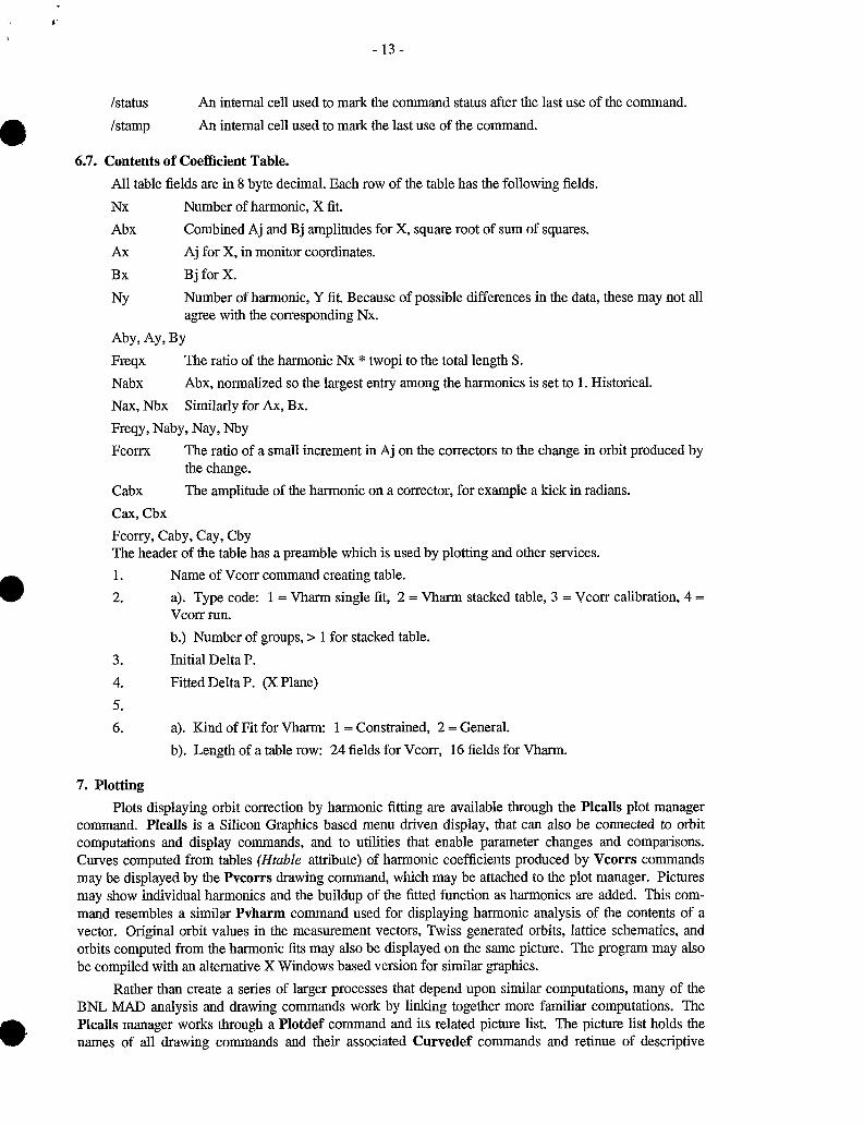
6.7. Contents of Coefficient Table. All table fields are in 8 byte decimal. Each row of the table has the following fields. Nx Abx Ax

Bx Bj for X.

NY

Number of harmonic, X fit. Combined Aj and Bj amplitudes for X, square root of sum of squares. Aj for X, in monitor coordinates.

Number of harmonic, Y fit. Because of possible differences in the data, these may not all agree with the corresponding Nx.

The ratio of the harmonic Nx * twopi to the total length S. Abx, normalized so the largest entry among the harmonics is set to 1. Historical. Similarly for Ax, Bx.

The ratio of a small increment in Aj on the correctors to the change in orbit produced by the change. The amplitude of the harmonic on a corrector, for example a kick in radians.

Aby, AY, BY Freqx Nabx Nax, Nbx

Freqy, Naby, Nay , m y Fcorrx

Cabx Cax, Cbx Fcorry, Caby, Cay, Cby The header of the table has a preamble which is used by plotting and other services. 1. 2.

Name of Vcorr command creating table. a). Type code: 1 = V h m single fit, 2 = Vharm stacked table, 3 = Vcorr calibration, 4 =

Vcorr run. b.) Number of groups, > 1 for stacked table.

Fitted Delta P. (X Plane)

a). Kind of Fit for Vharm: 1 = Constrained, 2 = General. b). Length of a table row: 24 fields for Vcorr, 16 fields for Vharm.

3. Initial Delta P. 4. 5. 6.

7. Plotting Plots displaying orbit correction by harmonic fitting are available through the Plcalls plot manager

command. Plcalls is a Silicon Graphics based menu driven display, that can also be connected to orbit computations and display commands, and to utilities that enable parameter changes and comparisons. Curves computed from tables (Htuble attribute) of harmonic coefficients produced by Vcorrs commands may be displayed by the Pvcorrs drawing command, which may be attached to the plot manager. Pictures may show individual harmonics and the buildup of the fitted function as harmonics are added. This command resembles a similar Pvharm command used for displaying harmonic analysis of the contents of a vector. Original orbit values in the measurement vectors, Twiss generated orbits, lattice schematics, and orbits computed from the harmonic fits may also be displayed on the same picture. The program may also be compiled with an alternative X Windows based version for similar graphics.

Rather than create a series of larger processes that depend upon similar computations, many of the BNL, MAD analysis and drawing commands work by linking together more familiar computations. The Plcalls manager works through a Plotdef command and its related picture list. The picture list holds the names of all drawing commands and their associated Curvedef commands and retinue of descriptive

- 14-

arrays. This supporting material is usually held on a separate call file, handled as a command library. Plcalls commands present a selection panel with a number of buttons, of which the Pick button presents a pop up menu holding the kinds (classes) of drawing commands submitted to the picture list by the program user. By selecting on a class, a further submenu is presented with the names of all drawing commands of that class, such as Pvcorrs. Selecting on one of these names leads to a corresponding Pvcorrs menu or drawing.

A number of drawings may share the same tracking and drawing commands and setups, presumably with considerable opportunities for producing mischief as well. Many of the drawing features push parts of the program rather further than they were designed to go. For example, values for corrector families may be changed by the drawing commands involved. If wanted, there are ways to restore lattice conditions by attaching appropriate set up and restore subroutines to the Plcalls Command list, which will display them for selection on a command submenu. In time, the more offensive shortcomings will be eased.

0

7.1. Pvcorrs Attributes vcorrs

Jharm

Menu

Masks

The Name of a Vcorrs command configured to produce a table of fitted harmonic coefficients or operate from an archived one. Integer noting a single harmonic to be displayed. Optional. If not given, the range of harmonics fitted by Vcorrs will be displayed. Ignored on Menu option. Logical Flag: If True, each harmonic to be displayed will be selected from a pop up menu. The Name of an optional integer may of masks (MAD Mvector form), keyed to har- monks. In non menu mode, if a mask array is given, only those harmonics for which the corresponding mask is greater than zero will be drawn. The drawing routine uses a drawing server directly attached to the Ftwiss command which computes orbits from the harmonic data. This server operates from a vector containing all 18 variables derived by the Twiss tracking at each element position. The variable(s) to be drawn, such as the closed orbit optics or displacements, are noted by positive values in an integer mask array keyed to the wanted variables. (ex. X = #11) All of the other Cur- vedef plotting service arrays are normally keyed to these variables in the Twiss vector, and so are not available to be keyed also to a particular harmonic. Hence an extra masking feature is provided for selecting out particular harmonics. A Name, X or Y , denoting which results to display from the harmonic table. Logical Flag: If True, the sums (synthesis) curves are not drawn. Can also be set from menu. Logical Flag: If True, the amplitude curves are not drawn. Can also be set from menu. Decimal values in pixels telling where the 1) amplitude and 2) sums curves are to be centered vertically, relative to inside (upper) edge of the lower border. Optional, but pictures can get very busy if both amplitude and synthesis curves lie about the same center.

Additional internal attributes are attached to the command stored in the data base. These items are supplied and used within the program. Acdef(2) Internal name group pointing to Curvedef command, which is linked through a

PldrawR command attached to a FTwiss command. The program traces all of these links. Internal name group pointing to default Pvcorrs command. Internal name group pointing to attached Vcorrs command. Internal name group pointing to attached Musks vector, if any. Internal decimal cells giving actual values for Ypos in plotting coordinates.

Xycode NoSums

NoAmps

Ypos(2)

Adefault(2) Avcorrs(2) Amasks(2)

/aY (2)

. . I

- 15-

/status, /stamp

7.2. PvcorrsMenu The Menu option presents a pop up menu with the following panels. The first three display the

currently selected harmonic Jharm, and the lowest (Jmin) and highest (Jmax) available. The set and change panels only modify Jharm; curves are produced only when the Return or All J panel is picked. Jharm =

Jmin =

Jmax =

Quit Vcorrs All J Return J + J - J = O J = Jmax J = Jmin Sums No Sums

Amps No Amps

Shows current value. Shows Jmin value. Shows Jmax value. Leaves current drawing routine and returns to main menu panel. Leaves menu to draw all J within Jmin - Jmax. Leaves menu to draw current Jharm. Increases Jharm by 1. Stays in menu. Decreases Jharm by 1. Sets Jharm to 0. Sets Jharm to Jmax. Sets Jharm to Jmin.

A toggle that displays current state of Sums (Synthesis curves) option, and switches it to alternate state.

@ Documentation

A toggle that displays current state of Amps (Amplitude curves) option, and switches it to alternate state.

Unix troff typeset format

Host:

This report:

Vharm Report:

Plcalls:

Vcorrs Test File:

Vcorrs Results:

rapt.ags.bnl.gov

/usr/disc2/jn/Docum+/Vcorrs.man

/usr/disc2/jn/Docum+/Vharm.man

/usr/disc2/jn/Docum+/Plcalls.man

/usr/disc2/jn/Docum+/Vcorrs.data

/usr/disc2/jn/Docum+/Vcorrs.print22

-. - - - __ _.- ~ __

Figure 1. The initial calibration fit to all data points produced by a Vcorrs command in the X plane. Data is

from an AGS Booster orbit snapshot taken in April of 1993 with a marked momentum offset of about -.0015 Data points are shown as crosses. The inside, more regular curve is the X displacement produced by the usual bare orbit application of the model. It simply doesn’t match the data very well. The average deviation here is about 7 mm per point. The second curve is the fit to the data produced by the calibration using the regular Booster corrector set. Nearly all of the penalty comes from points about A2 and C8. - _ _ -

- 17 -

The upper curves are individual harmonic amplitudes which contribute to the synthesis curves. J = 4 1 7 I l - . . : . . . L .

- 18 -

Figure 3. I '

, I

Synthesis and amplitude curves similar to Figure 2, computed using a calibration from which errant '

data points A2 and C8 have been omitted. - .- . ~..

_ _ - - -

Figure 4. Amplitude curves for harmonic J = 5, computed using calibrations with and without errant data

points A2 and C8. The curves show the reduction of the orbit displacement caused by placing this fifth harmonic on the correctors for the two cases, for negligible momentum offset. The phase is not affected. - - -

Figure 5. Comparison of fits to measured data points by the constrained harmonic method (heavy curve) and

the corrector calibration method of this paper (thin curve). The latter produces better detail, especially at the extraction region. The upper curves compare the apparent J = 9 amplitudes. The correction curve is phase reversed relative to the plain fit.

a

- 21 - + I

1 Vcorrs Command L i b r a r y f o r Booster Runs 1 February 21 , 1 9 9 7 I F i l e = 11/usr/disc2/jn/Docum+/Vcorrs. d a t a " ! P a r t of: 11/usr/disc2/jn/Booster+/Hruns. boost1

0 . . . . . . . . . . . . . . . . . . . . . . . . . . . . . . . . . . . . . . . . . . . . . . . . . . . . . . . . . . . . . . . . . . . . . . P d e l t a Param = - .001462 S to re ! C a l i b r a t i o n Mode Command, Arrays, and R e l a t e d Commands. Boos-C20 Vcorrs C a l i b , Bpmdata = I1X Data",

Bpms = L - XBPM, C o r r s = L - XKICK, Weights = I1X - Wgts2OI1, Factors = I1X Facts' ', P r i n t , C y c l e s = 1;10,3, C o n v e r t = .001, Fi l te r = 9 9 9 . , BParams = I1/X I /Y I

CParams = I1/Dpx I I1 /Dpy I

T w i s s = FTW-Cal, Htable = IIHc t ab l e" , Csave = I1C - savC2Ol1, P s a v e = I I P - Zav~2011, Jmin = 1, Jmax = 9 , Smax = 201.78

11 11

I1 11

I1X D a t a l ' Vector, 3.356113 -8.693634 -4.038608 1 .899860 1 .212470 -4.886150

-7.630552 -1.532651 2.786204 0.946376 -7.146722 -19.704966 -4.802379 -1.614516 44444. -0 .625031 -5.475378 -4.604772 -2.491268 -0.376475 -2 .166401 -4.313535 44444. 1 .058067

I S u p p r e s s A2, C8 f o r C a l i b r a t i o n ==> 20 P o i n t s . I1X Wgts201' Vector 24 lOOOOOO., Value(1) = O . , V a l u e ( l 2 ) = 0 . llX-Factsll Vector 24 .01 FTW G a l F twiss , Deltap = p d e l t a rch C20 Archive I1C savC20g1, IlP savC2Oll 6 - trv-C20 R e t r i e v e Force, 11C-savC2011, - 11P-savC2011 -

I************************************************************************

! Running Mode Command, A r r a y s , and Re la t ed Commands'. Boos-R20 Vcorrs Bpmdata = I1X Data",

Bpms = L - KBPM, C o r r s = L - XKICK, Weights = I IX-Wgts I r , Factors = llX-Factsll, P r i n t , C y c l e s = 1 , 1 0 , 3 , BParams = I1/X I / Y I

CParams = I1/Dpx I /Dpy ?

11 I1

11 11

T w i s s = FTW Run, Htable = 11Brun-R2011, Csave = 'IC - E ~ v R ~ O ~ ~ , P s a v e = IIP - savR20t1 , Smax = 201 .78 , Jmin = 1, Jmax = 9

& & & & & & & & & &

& & & &

& & & & & & & & &

llX-WgtS1l Vector = 24 1000000 . A r c h R20 Archive I1P savR20f1 , "Brun R20" Rtrv-R20 R e t r i e v e Force, 11P-savR2011, 11BrunIR2011

L i s t = L - XKICK, Param = ''KICK FTW .Run F twis s , Deltap = I1P - savC20I1

"VtOD-C20 I' V t o D L i s t = LZKICK, Param = I~KICK , Vname = !IC savC20f1 "VtoDR20 " V t o D 1 1 , Vname = 11C'-savR2011 -

. . . . . . . . . . . . . . . . . . . . . . . . . . . . . . . . . . . . . . . . . . . . . . . . . . . . . . . . . . . . . . . . . . . . . . . . .

1 Drawing Commands f o r Synthes is , A m p l i t u d e C u r v e s . = T.BoS-Rl, & P V c o r r s Vcorrs

& xycode = x, Menu, Cvcor ypos = Yyused * .50, Yyused * .75 I Vcorrs Command f o r Drawing Resul t s i n C o e f f i c i e n t T a b l e .

& T.Bos - R 1 Vcorrs Bpms = L - XBPM, C o r r s = L - XKICK,

1WAOll Vers io 9 7.63-BNL/UNIX Copyr ight (C) 1988 by CERN. Date and Time o f Th is Run: 02/20/97 1 7 : l O : l l

800S-C22 ! ! Begin C a l i b r a t i o n f o r A L L 22 Points .

LINEAR LATTICE PARAMETERS FOR BEAM LINE: "BOOSTER I t , RANGE = W S / #E" OELTA(P)/P = -0.001462 symm = F PAGE 1 ____________________---------------------------------.----------------------------------------------------------------------------

ELEMENT SEQUENCE I H O R I Z O N T A L I V E R T I C A L POS. ELEMENT OCC. OIST I BETAX ALFAX MUX X(C0) PX(C0) OX OPX I BETAY ALFAY MUY Y(C0) PY(C0) OY OPY NO. NAME NO. [ M I 1 [ M I I 1 1 C2PIl [MMI [.0011 [ M I [ I 1 1 [ M I [ I 1 [ P P I 1 [MMI [ . o O l l [ M I [11 _______--------_------------------.----------------------------------------------------------------------------------------------- BEGIN BOOSTER 1 0.000 5.412 0.980 0.000 -0.956 0.138 0.644-0.093 9.755 -1.556 0.000 0.000 0.000 0.000 0.000 EN0 BOOSTER 1 201.780 5.412 0.980 4.810 -0.956 0.138 0.644-0.093 9.754 -1.556 4.806 0.000 0.000 0.000 0.000

TOTAL LENGTH = 201.780000 QX - 4.809952 QY - 4.806365 OELTA(S) = -1 2.434270 mm QX' - -7.268288 QY' - -3.01 0743 ALFA - 0.419520E-01 BETAX(MAX) = 13.566733 BETAY(MAX) = 13.671 140 GAMMA(TR) = 4.882290 OX(MAX) - 2.966057 OY(MAX) - 0 .oooooo

XCO(MAX) = 4.327952 YCO(h4AX) = XCO(R.M.S.) = 2.546150 YCO(R.M.S.) = 0.000000

. . . . . . . . . . . . . . . . . . . . . . . . . . . . . . . . . . . . . . . . . . . . . . . . . . . . . . . . . . . . . . . . . . . . . . . . . . . . . . . . . . . . . . . . . . . . . . . . . . . . . . . . . . . . . . . . . . . . . . . . . . . . . . . . . . - - - -

- - -

0 .oooooo

Harmonics Program. S t a r t i n g Value f o r WOsq = X Harm A B Lsq

Begi n -0.001 462 507.91 End Del tap 0 -0.001621 0.000000 505.56 End Harmonic 5 -0.003184 0.001788 281.64 End Harmonic 4 -0.001594 0.000509 201 .75 End Harmonic 6 0.000384 -0.000620 190.11 End Harmonic 3 0.001346 -0.000419 139.47 End Harmonic 7 -0.000761 0.000050 123.99 End Harmonic 2 -0.000791 0.000383 104.20 End Harmonic 8 -0.000394 -0.000831 80.59 End Harmonic 1 0.001005 0.000061 53.89 End Harmonic 9 -0.000597 0.000326 40.56

I t e r a t i o n 1, Penal ty 40.56, Pen Change

N Moni tor S V Measured V F i t t e d 1 PUEHA2 5.08 0.003956 0.002325

Summary Table f o r X C a l i b r a t i o n F i t s .

2 PUEHA4 13.49 -0.008694 -0.007924 3 PUEHA6 21 .90 -0.004039 -0.005597 4 PUEHAB 30.30 0.001900 0.001944 5 PUEHBZ 38.71 0.001212 0.001407 6 PUEHB4 47.12 -0.004886 -0.005102 7 PUEHB6 55.53 -0.007631 -0.007438 8 PUEHB8 63.93 -0.001 533 -0.002244 9 PUEHC2 72.34 0.002786 0.002442

10 PUEHC4 80.75 0.000946 0.001 633 11 PUEHC6 89.16 -0.0071 47 -0.009463 12 PUEHC8 97.56 -0.01 9705 -0.01 7886 13 PUEHD2 105.97 -0.004802 -0.007360 14 PUEHO4 11 4.38 -0.001 61 5 0.001 033 15 PUEHO6 122.79 0.000000 0.000368 16 PUEHO8 131 .19 -0.000625 0.0001 00 17 PUEHE2 139.60 -0.005475 -0.005806 18 PUEHE4 148.01 -0.004605 -0.005918 19 PUEHE6 156.42 -0.002491 -0.000869 20 PUEHE8 164.82 -0.000376 -0.002086

507.908 Time

17:10:18 17:lO: 22 17:10:31 17: l0 :38 17: 10: 45 17: 10:53 17: 11 :01 17 :11:08 17:11:15 17:11:23 17:11:31

-467.35.

Oi f ference 0.001 631

0.001 558 -0.000769

-0.000045 -0.0001 95 0.00021 6

0.00071 2 0.000345

0.00231 6

0.002558 -0.002648 0.000000

-0.000725 0.000331 0.001313

0.001 710

-0.0001 92

-0.000686

-0.001 81 9

-0.001622

Mean Oev. Change

2.349 223.924

79.890 11.637 50.640 15.482 19.788 23.610 26.695 13.334

Or ig Oev.

Pena Lty 2.661 0.592 2.428 0.002 0.038 0.046 0.037 0.506 0.119 0.471 5.364 3.309 6.543 7.010 0.000 0.526 0.110 1.724 2.632 2.924

- - 0.0048 Passes

7 14 13 13 13 13 13 13 13 13

-0.000320, Oev Change

Weight 1000000.000 1000000.000 1000000.000 1000000.000 1000000.000 1000000.000 1000000.000 1000000.000 1000000.000 1000000.000 1000000.000 1000000.000 1000000.000 1000000.000 1000000.000 1000000.000 1000000.000 1000000.000 1000000.000 1000000.000

V I n i t i a l -0.001 654 -0.004003 -0.004194 -0.001 748 -0.001 654 -0.004003 -0.0041 94 -0.001748 -0.001654 -0.004003 -0.004194 -0.001 748 -0.001 654 -0.004003 -0.0041 94 -0.001748 -0.001654 - 0.004003 -0.004194 -0.001 748

I N N

I

-0.000320

V Change 0.003979

-0.003921 -0.001 403 0.003692 0.003061

-0.001099 -0.003244 -0.000497 0.004096 0.005636

-0.005269 -0.016138 -0.005706 0.005036 0.004562 0.001 848

-0.004152 -0.001915

-0.000339 0.003325

21 PUEHF2 173.23 -0.0021 66 -0.001 929 -0.000238 0.056 1000000.000 -0.001654 -0.000275

181 .64 -0.004314 -0.004678 0.000364 0.133 000.000 -0.004003 -0.000675 e 23 PUEHF6 190.05 0.000000 -0.006774 0.000000 0.000 1000000.000 -0.004194 -0.002580 24 PUEHFB 198.45 0.001 058 0.002883 -0.001 825 3.330 1000000.000 -0.001748 0.004630 I t e r = 1 F i n a l Lsq = 40.560 Mean Dev. = 0.001358

I n i t i a L Lsq = 507.908 Mean Dev. = 0.004805 Summarv Table f o r X Correctors Ca l i b ra t i on .

N Corrector S 1 DHCA2 4.77 2 DHCA4 13.18 3 DHCA6 21.59 4 DHCA8 30.00 5 DHCB2 38.40 6 DHCB4 46.81 7 DHCB6 55.22 8 DHCB8 63.63 9 DHCC2 72.03

10 DHCC4 80.44

12 DHCC8 97.26 13 DHCD2 105.66 14 DHCD4 114.07 15 DHCD6 122.48 16 DHCD8 130.89 17 DHCEZ 139.29 18 DHCE4 147.70 19 DHCE6 156.11 20 DHCE8 164.52 21 DHCF2 172.92 22 DHCF4 181.33 23 DHCF6 189.74 24 DHCF8 198.15

RAW FOURIER STRENGTHS I N X. Y

11 DHCC6 88.85

C F i t t e d -0.0001 02 0.000470 0.000083 0.000004 0.0001 18 0.000071 0.000071 0.0001 43 0.000293

-0.000376 -0.000570 -0.000086 -0.000644 -0.000353 0.000372

-0.000025 0.000250 0.000081

-0.000369 0.000328

-0.000024 -0.0001 97

-0.000060 0.000520

C I n i t i a l 0.000000 0.000000 0.000000 0.000000 0.000000 0.000000 0.000000 0.000000 0.000000 0.000000 0.000000 0.000000 0.000000 0.000000 0.000000 0.000000 0.000000 0.000000 0.000000 0.000000 0.000000 0.000000 0.000000 0.000000

Dif ference -0.000102 0.000470 0.000083 0.000004 0.0001 18 0.000071 0.000071 0.0001 43 0.000293

-0.000376 -0.000570 -0.000086 -0.000644 -0.000353

-0.000025 0.000372

0.000250 0.000081

0.000328 -0.000369

-0.000024 -0.0001 97 0.000520

-0.000060

Fact or s 0.100000 0.100000 0.100000 0.100000 0.100000 0.100000 0.100000 0.100000 0.100000 0.100000 0.100000 0.100000 0.100000 0.100000 0.100000 0.100000 0.100000 0.100000 0.100000 0.100000 0.100000 0.100000 0.100000 0.100000

NORMALIZED FOURIER STRENGTHS I N X. Y N FREQ(N) ABX(N) AX(N) BX(N) N ABY(N) AY(N) BY(N) N ABX(N) AX(N) BX(N) N ABY(N) AY(N) BY(N) 0 0.00000 0.00000 0.00000 0.00000 0 0.00000 0.00000 0.00000 0 0.00000 0.00000 0.00000 0 0.00000 0.00000 0.00000 1 0.03114 0.00101 0.00101 0.00006 0 0.00000 0.00000 0.00000 1 0.27574 0.27524 0.01666 0 0.00000 0.00000 0.00000 2 0.06228 0.00088 -0.00079 0.00038 0 0.00000 0.00000 0.00000 2 0.24077 -0.21672 0.10489 0 0.00000 0.00000 0.00000 3 0.09342 0.00141 0.00135 -0.00042 0 0.00000 0.00000 0.00000 3 0.38599 0.36857 -0.11467 0 0.00000 0.00000 0.00000 4 0.12456 0.00167 -0.00159 0.00051 0 0.00000 0.00000 0.00000 4 0.45804 -0.43636 0.13927 0 0.00000 0.00000 0.00000 5 0.15569 0.00365 -0.00318 0.00179 0 0.00000 0.00000 0.00000 5 1.00000 -0.87189 0.48970 0 0.00000 0.00000 0.00000 6 0.18683 0.00073 0.00038 -0.00062 0 0.00000 0.00000 0.00000 6 0.19978 0.10515 -0.16987 0 0.00000 0.00000 0.00000 7 0.21797 0.00076 -0.00076 0.00005 0 0.00000 0.00000 0.00000 7 0.20881 -0.20836 0.01371 0 0.00000 0,00000 0.00000 8 0.24911 0.00092 -0.00039 -0.00083 0 0.00000 0.00000 0.00000 8 0.25179 -0.10802 -0.22745 0 0.00000 0.00000 0.00000 9 0.28025 0.00068 -0.00060 0.00033 0 0.00000 0.00000 0.00000 9 0.18622 -0.16342 0.08929 0 0.00000 0.00000 0.00000

LINEAR LATTICE PARAMETERS FOR BEAM LINE: "BOOSTER !I, RANGE = "#S / #E" DELTA(P)/P = -0.001621 symm = F PAGE 1 . . . . . . . . . . . . . . . . . . . . . . . . . . . . . . . . . . . . . . . . . . . . . . . . . . . . . . . . . . . . . . . . . . . . . . . . . . . . . . . . . . . . . . . . . . . . . . . . . . . . . . . . . . . . . . . . . . . . . . . . . . . . . . . . . . . . . . . . . . . . . . . . . . . . . . . . . . . .

ELEMENT SEQUENCE I H O R I Z O N T A L I V E R T I C A L POS. ELEMENT OCC. D I S T I BETAX ALFAX MUX X(C0) PX(C0) DX DPX I BETAY ALFAY MUY Y(C0) PY(C0) DY DPY I ELEMENT LENGTH STRENGTH NO. NAME NO. [ M I 1 [ M I C11 C2PIl [MMI [ * o O l l [ M I 111 1 [ M I [ I 1 12PII [MMI C.0011 [MI [ I 1

BEGIN BOOSTER 1 0.000 5.447 0.983 0.000 2.586 -0.387 0.507-0.062 9.695 -1.547 0.000 0.000 0.000 0.000 0.000 END BOOSTER 1 201.780 5.447 0.983 4.811 2.586 -0.387 0.507-0.062 9.694 -1.547 4.807 0.000 0.000 0.000 0.000

TOTAL LENGTH = 201 .780000 QX - 4.81 11 05 QY - 4.806699 DELTA(S) = -13.972943 mm QX' -7.267469 QY' - -3.011682 ALFA - 0.419143E-01 BETAX(MAX) = 13.611467 BETAY(MAX) = 13.675287 GAMMA(TR) = 4.884488 DX(MAX) - 3.09771 0 DY(MAX) - 0.000000

XCO(MAX) = 18.179518 YCO(MAX) = 0.000000 XCO(R.M.S.) = 4.722295 YCO(R.M.S.) = 0.000000

. . . . . . . . . . . . . . . . . . . . . . . . . . . . . . . . . . . . . . . . . . . . . . . . . . . . . . . . . . . . . . . . . . . . . . . . . . . . . . . . . . . . . . . . . . . . . . . . . . . . . . . . . . . . . . . . . . . . . . . . . . . . . . . . . . . . . . . . . . . . . . . . . . . . . . . . . . . .

. . . . . . . . . . . . . . . . . . . . . . . . . . . . . . . . . . . . . . . . . . . . . . . . . . . . . . . . . . . . . . . . . . . . . . . . . . . . . . . . . . . . . . . . . . . . . . . . . . . . . . . . . . . . . . . . . . . . . . . . . . . . . . . . . . . . . . . . . . . . . . . . . . . . . . . . . . . . - - = -

- - -

__-_____________________________________--------------------------------------------------------------------------------------------.-----------------------

BOOS-R22 ! ! Begin Correct ion Run. ALL Points.

LINEAR LATTICE PARAMETERS FOR BEAM LINE: "BOOSTER I t , RANGE = "#S / #E" OELTA(P)/P = 0.000000 symm = F PAGE 1

ELEMENT SEQUENCE I

NO. NAME NO. [ M I 1 [ M I

BEGIN BOOSTER 1 0.000 5.444 EN0 BOOSTER 1 201.780 5.444

TOTAL LENGTH = 201.780000 OELTA(S) = -0.189805 mm ALFA - 0.423552E-01 GAMMA(TR) = 4.858995

POS. ELEMENT OCC. O I S T I BETAX

. . . . . . . . . . . . . . . . . . . . . . . . . . . . . . . . . . . . . . .

. . . . . . . . . . . . . . . . . . . . . . . . . . . . . . . . . . . . . . .

-

V E R T I C A L BETAY ALFAY MUY Y(C0) PY(C0) OY DPY [ M I [ I 1 [ 2 P I I [MMI C.0011 [ M I [ I 1 . _ _ _ - _ _ _ _ _ _ _ - - _ _ _ _ _ _ _ _ _ _ _ _ _ _ _ _ _ _ _ _ _ _ _ _ _ _ - - - - - - - - - 9.701 -1.548 0.000 0.000 0.000 0.000 0.000 9.701 -1.548 4.802 0.000 0.000 0.000 0.000 ._----________._____-----------.-------.---------

- QY - 4.801815 BY' -2.9881 17 BETAY(MAX) = 13.671588 OY(MAX) - 0.000000 YCO(MAX) = 0.000000 YCO(R.M.S.) = 0.000000

- - -

ELEMENT LENGTH STRENGTH

Harmonics Program. S t a r t i n g Value f o r WDsq = X Harm A B Lsq

Begin 0.000000 513.79 End Oeltap 0 0.000034 0.000000 513.17 End Harmonic 5 0.003655 -0.001725 258.90 End Harmonic 4 0.001538 -0.000573 170.77 End Harmonic 6 -0.000404 0.000600 158.82 End Harmonic 3 -0.001296 0.000403 104.79 End Harmonic 7 0.000721 -0.000048 89.48 End Harmonic 2 0.000775 -0.000369 68.06 End Harmonic 8 0.000403 0.000843 43.77 End Harmonic 1 -0.000926 -0.000048 19.27 End Harmonic 9 0.000626 -0.000343 3.62

Summary Table f o r X Adjustment F i t s . I t e r a t i o n 1, Penal ty 3.62, Pen Change

N 1 2 3 4 5 6 7 8 9

10 11 12 13 14 15 16 17 18 19 20 21 22 23

Monitor PUEHA2 PUEHA4 PUEHA6 PUEHA8 PUEHB2 PUEHB4 PUEHB6 PUEHB8 PUEHC2 PUEHC4 PUEHC6 PUEHC8 PUEHO2 PUEHD4 PUEHO6 PUEHO8 PUEHE2 PUEHE4 PUEHE6 PUEHE8 PUEHFZ PUEHF4 PUEHF6

S 5.08

13.49 21.90 30.30 38.71 47.12 55.53 63.93 72.34 80.75 89.16 97.56

105.97 114.38 122.79 131.19 139.60 148.01 156.42 164.82 173.23 181.64 190.05

Good Orb; t 0.000000 0.000000 0.000000 0.000000 0.000000 0.000000 0.000000 0.000000 0.000000 0.000000 0.000000 0.000000 0.000000 0.000000 0.000000 0.000000 0.000000 0.000000 0.000000 0.000000 0.000000 0 .oooooo 0.000000

V F i t t e d

0.000242 0.000675 0.000369

-0.000264 -0.000262

-0.00031 6

0.000283 0.000443

-0.000051 -0.000402 -0.0001 46 0.000266 0.0001 98

-0.00031 1 -0.000500 0.000040 0.000622 0.000332 - 0.000405

-0.000530 0.000201 0.000759 0.000461

513.787 Time

17:11:33 17:11:37 17: 11 :44 17:11:52 17: 12:OO 17: 12:07 17:12:15 17:12:22 17:12 :30 17 : 12:37 17: 12:45

-510.17,

Di f ference 0.00031 6

-0.000242 -0.000675 -0.000369 0.000264 0.000262

-0.000283 -0.000443 0.00005 1 0.000402 0.0001 46

-0.000266 -0.000198 0.00031 1 0.000500

-0.000040 -0.000622 -0.000332 0.000405 0.000530

-0.000201 -0.000759 -0.000461

Mean Dev. = 0.0046. Change Passes

0.616 6 254.268 14 88.129 13 11.949 13 54.033 13 15.310 13 21.423 13 24.284 13 24.499 13 15.655 13

Or ig Oev. -0.000009, Oev Change -0.000009

Penalty 0.100 0.059 0.456 0.136 0.070 0.069 0.080 0.197 0.003 0.162 0.021 0.071 0.039 0.097 0.250 0.002 0.386 0.110 0.164 0.280 0.041 0.575 0.213

Weight 1000000.000 1000000.000 1000000.000 1000000.000 1000000.000 1000000.000 1000000.000 1000000.000 1000000.000 1000000.000 1000000.000 1000000.000 1000000.000 1000000.000 1000000.000 1000000.000 1000000.000 1000000.000 1000000.000 1000000.000 1000000.000 1000000.000 1000000.000

V I n i t i a l 0.004021

-0.00321 4 -0.000679 0.003771 0.002936

-0.00071 6 -0.002531 -0.0001 02 0.0041 35 0.005794

-0.004804 -0.015662 -0.005457 0.00521 4 0.004833 0.0021 92

-0.003689 -0.001500 0.003478

0.0001 04 0.000030

-0.000297

-0.0021 46

V Change -0.004338 0.003455 0.001 355

-0.003402 -0.003200 0.000454 0.00281 4 0.000546

-0.004186 -0.0061 96 0.004658 0.01 5928 0.005655

-0.005525 -0.005333 -0.0021 52 0.00431 0 0.001 833

-0.003883 -0.000233 0.000097 0.000729 0.002608

Adj O i f f . 0.000379

-0.0001 79 -0.000613 -0.000306 0.000327 0.000325

-0.000220 -0.000381 0.0001 13 0.000465 0.000209

-0.000203 -0.000135 0.000374 0.000562 0.000023

- 0.000559 -0.000269 0.000467 0.000592

-0.000139 -0.000696 -0.000399

I N c

I

Adj Pen. 0.144 0.032 0.376 0.094 0.107 0.105 0.049 0.145 0.013 0.216 0.044 0.041 0.018 0.140 0.316 0.001 0.312 0.073 0.218 0.351 0.019 0.484 0.159

24 PUEHi-o a 198.45 0.000000 -0.000201 I t e r = 1 F i n a l L s q = 3.620 Mean D e v . = A d j u s t e d : F i n a l L s q = 3.525 Mean D e v . =

I n i t i a l L s q = 513.787 Mean D e v . = Summary T a b l e f o r X C o r r e c t o r s Run .

N C o r r e c t o r S C F i t t e d C I n i t i a l 1 OHCA2 4.77 0.000010 -0.000102 2 DHCA4 13.18 0.000012 0.000470 3 OHCA6 21.59 0.000008 0.000083 4 OHCAB 30.00 0.000007 0.000003 5 DHCBZ 38.40 0.000014 0.000118 6 OHCB4 46.81 0.00001 0 0.000070 7 OHCB6 55.22 -0.000007 0.000071 8 OHCB8 63.63 -0.00001 2 0.0001 43 9 DHCC2 72.03 -0.000003 0.000293 10 OHCC4 80.44 -0.000001 -0.000377 11 DHCC6 88.85 -0.000009 -0.000571 12 OHCC8 97.26 -0.000018 -0.000086 13 OHCO2 105.66 -0.000023 -0.000644 14 OHCD4 1 1 4.07 -0.00001 6 -0.000353 15 OHC06 122.48 -0.000001 0.000372 16 OHCD8 130.89 0.000000 -0.000025 17 DHCE2 139.29 -0.000009 0.000250 18 DHCE4 147.70 -0.000007 0.000081 19 OHCE6 156.11 0.000001 -0,000369 20 OHCEl 164.52 0.000000 0 .a00328 21 OHCF2 172.92 -0.000001 -0.000024 22 DHCF4 181 .33 0.000009 -0.0001 97

24 DHCF8 198.15 0.000013 -0.000060 23 DHCF6 189.74 0.00001 7 0.000520

RAW FOURIER STRENGTHS I N X, Y

0.000201 0.000388 0.000383 0.004627

C h a n g e 0.00011 2 -0.000458 -0.000075 0.000003 -0.0001 04 -0.000060 -0.000077 -0.000155 -0.000296 0.000376 0.000561 0.000068 0.000621 0.000337

0.000025 -0.000372

-0.000259 -0.000088 0.000370

0.000023 0.000206

0.000072

-0.000328

-0.000504

0.040 000.000 0.004498 -0.004699 0.000264 0.070 A v e G = 0.000000 A v e B = 0.000063

F a c t or s 0.100000 0.100000 0.100000 0.100000 0.100000 0.100000 0.100000 0.100000 0.100000 0.100000 0.100000 0.100000 0.100000 0.100000 0.100000 0.100000 0.100000 0.100000 0.100000 0.100000 0.100000 0.100000 0.100000 0.100000

NORMALIZED FOURIER STRENGTHS I N X, Y N FREQ(N) ABX(N) AX(N) BX(N) N ABY(N) AY(N) BY(N) N ABX(N) AX(N) BX(N) N ABY(N) AY(N) BY(N) 0 0.00000 0.00000 0.00000 0.00000 0 0.00000 0.00000 0.00000 0 0.00000 0.00000 0.00000 0 0.00000 0.00000 0.00000 1 0.03114 0.00093 -0.00093 -0.00005 0 0.00000 0.00000 0.00000 1 0.22943 -0.22913 -0.01179 0 0.00000 0.00000 0.00000 2 0.06228 0.00086 0.00077 -0.00037 0 0.00000 0.00000 0.00000 2 0.21232 0.19168 -0.09131 0 0.00000 0.00000 0.00000 3 0.09342 0.00136 -0.00130 0.00040 0 0.00000 0.00000 0.00000 3 0.33576 -0.32065 0.09960 0 0.00000 0.00000 0.00000 4 0.12456 0.00164 0.00154 -0.00057 0 0.00000 0.00000 0.00000 4 0.40606 0.38050 -0.14179 0 0.00000 0.00000 0.00000 5 0.15569 0.00404 0.00366 -0.00173 0 0.00000 0.00000 0.00000 5 1.00000 0.90431 -0.42688 0 0.00000 0.00000 0.00000 6 0.18683 0.00072 -0.00040 0.00060 0 0.00000 0.00000 0.00000 6 0.17892 -0.09985 0.14846 0 0.00000 0.00000 0.00000 7 0.21797 0.00072 0.00072 -0.00005 0 0.00000 0.00000 0.00000 7 0.17869 0.17829 -0.01182 0 0.00000 0.00000 0.00000 8 0.24911 0.00093 0.00040 0.00084 0 0.00000 0.00000 0.00000 8 0.23124 0.09967 0.20865 0 0.00000 0.00000 0.00000 9 0.28025 0.00071 0.00063 -0.00034 0 0.00000 0.00000 0.00000 9 0.17666 0.15499 -0.08477 0 0.00000 0.00000 0.00000

L INEAR L A T T I C E PARAMETERS FOR BEAM L I N E : "BOOSTER I t , RANGE = "#S / #E" DELTA(P) /P = 0.000034 symm = F PAGE 1 . . . . . . . . . . . . . . . . . . . . . . . . . . . . . . . . . . . . . . . . . . . . . . . . . . . . . . . . . . . . . . . . . . . . . . . . . . . . . . . . . . . . . . . . . . . . . . . . . . . . . . . . . . . . . . . . . . . . . . . . . . . . . . . . . . . . . . . . . . . . . . . . . . . . . . . . . . . .

ELEMENT SEQUENCE I H O R I Z O N T A L I V E R T I C A L POS. ELEMENT OCC. O I S T I BETAX ALFAX MUX X(C0) PX(C0) OX OPX I BETAY ALFAY MUY Y(C0) PY(C0) OY DPY I ELEMENT LENGTH STRENGTH NO. NAME NO. [MI 1 [MI [11 [2PIl CMMI [.0011 [MI r.11 1 [MI 1 1 1 [ 2 P I I CMMI [.Ooll [MI [ I 1 -_____----______-___-----------------.---------------------------------------------------------------------------------------------------------------------- BEGIN BOOSTER 1 0.000 5.409 0.978 0.000 -0.198 0.013 0.676-0.097 9.762 -1.557 0.000 0.000 0.000 0.000 0.000 END BOOSTER 1 201.780 5.409 0.978 4.799 -0.198 0.013 0.676-0.097 9.762 -1.557 4.802 0.000 0.000 0.000 0.000

TOTAL LENGTH = 201 .780000 QX - 4.799098 QY - 4.801 866 DELTA(S) = 0.298352 mm QX' - -7.274935 QY' - -2.989095 ALFA - 0.423541E-01 BETAX(MAX) = 13.566623 BETAY(MAX) = 13.666313 GAMMA(TR) = 4.859063 DX(MAX) - 2.965588 OY(MAX) - 0.000000

XCO(MAX) = 0.779494 YCO(MAX) = 0.000000 XCO(R.M.S.) = 0.312237 YCO(R.M.S.) = 0.000000

. . . . . . . . . . . . . . . . . . . . . . . . . . . . . . . . . . . . . . . . . . . . . . . . . . . . . . . . . . . . . . . . . . . . . . . . . . . . . . . . . . . . . . . . . . . . . . . . . . . . . . . . . . . . . . . . . . . . . . . . . . . . . . . . . . . . . . . . . . . . . . . . . . . . . . . . . . . . - - - -

- - -

. . . . . . . . . . . . . . . . . . . . . . . . . . . . . . . . . . . . . . . . . . . . . . . . . . . . . . . . . . . . . . . . . . . . . . . . . . . . . . . . . . . . . . . . . . . . . . . . . . . . . . . . . . . . . . . . . . . . . . . . . . . . . . . . . . . . . . . . . . . . . . . . . . . . . . . . . . . .

bnl mad harmonic analysis based orbit correction … notes/tn456.pdf · minimizes the least squares...

Documents