bond risk premia - stanford university
TRANSCRIPT

Bond Risk Premia
By JOHN H COCHRANE AND MONIKA PIAZZESI
We study time variation in expected excess bond returns We run regressions ofone-year excess returns on initial forward rates We find that a single factor asingle tent-shaped linear combination of forward rates predicts excess returns onone- to five-year maturity bonds with R2 up to 044 The return-forecasting factor iscountercyclical and forecasts stock returns An important component of the return-forecasting factor is unrelated to the level slope and curvature movements de-scribed by most term structure models We document that measurement errors donot affect our central results (JEL G0 G1 E0 E4)
We study time-varying risk premia in USgovernment bonds We run regressions of one-year excess returnsndashborrow at the one-year ratebuy a long-term bond and sell it in one yearndashonfive forward rates available at the beginning ofthe period By focusing on excess returns wenet out inflation and the level of interest ratesso we focus directly on real risk premia in thenominal term structure We find R2 values ashigh as 44 percent The forecasts are statisti-cally significant even taking into account thesmall-sample properties of test statistics andthey survive a long list of robustness checksMost important the pattern of regression coef-ficients is the same for all maturities A singleldquoreturn-forecasting factorrdquo a single linear com-bination of forward rates or yields describestime-variation in the expected return of allbonds
This work extends Eugene Fama and RobertBlissrsquos (1987) and John Campbell and Robert
Shillerrsquos (1991) classic regressions Fama andBliss found that the spread between the n-yearforward rate and the one-year yield predicts theone-year excess return of the n-year bond withR2 about 18 percent Campbell and Shillerfound similar results forecasting yield changeswith yield spreads We substantially strengthenthis evidence against the expectations hypothe-sis (The expectations hypothesis that longyields are the average of future expected shortyields is equivalent to the statement that excessreturns should not be predictable) Our p-valuesare much smaller we more than double theforecast R2 and the return-forecasting factordrives out individual forward or yield spreads inmultiple regressions Most important we findthat the same linear combination of forwardrates predicts bond returns at all maturitieswhere Fama and Bliss and Campbell andShiller relate each bondrsquos expected excess re-turn to a different forward spread or yieldspread
Measurement ErrormdashOne always worriesthat return forecasts using prices are contami-nated by measurement error A spuriously highprice at t will seem to forecast a low return fromtime t to time t 1 the price at t is common toleft- and right-hand sides of the regression Weaddress this concern in a number of ways Firstwe find that the forecast power the tent shapeand the single-factor structure are all preservedwhen we lag the right-hand variables runningreturns from t to t 1 on variables at timeti12 In these regressions the forecasting
Cochrane Graduate School of Business University ofChicago 5807 S Woodlawn Ave Chicago IL 60637 (e-mail johncochranegsbuchicagoedu) and NBER Pi-azzesi Graduate School of Business University of Chicago5807 S Woodlawn Ave Chicago IL 60637 (e-mailmonikapiazzesigsbuchicagoedu) and NBER We thankGeert Bekaert Michael Brandt Pierre Collin-DufresneLars Hansen Bob Hodrick Narayana Kocherlakota PedroSanta-Clara Martin Schneider Ken Singleton two anony-mous referees and many seminar participants for helpfulcomments We acknowledge research support from theCRSP and the University of Chicago Graduate School ofBusiness and from an NSF grant administered by theNBER
138
variables (time ti12 yields or forward rates)do not share a common price with the excessreturn from t to t 1 Second we compute thepatterns that measurement error can produceand show they are not the patterns we observeMeasurement error produces returns on n-periodbonds that are forecast by the n-period yield Itdoes not produce the single-factor structure itdoes not generate forecasts in which (say) thefive-year yield helps to forecast the two-yearbond return Third the return-forecasting factorpredicts excess stock returns with a sensiblemagnitude Measurement error in bond pricescannot generate this result
Our analysis does reveal some measurementerror however Lagged forward rates also helpto forecast returns in the presence of time-tforward rates A regression on a moving aver-age of forward rates shows the same tent-shapedsingle factor but improves R2 up to 44 percentThese results strongly suggest measurement er-ror Since bond prices are time-t expectations offuture nominal discount factors it is very diffi-cult for any economic model of correctly mea-sured bond prices to produce dynamics in whichlagged yields help to forecast anything If how-ever the risk premium moves slowly over timebut there is measurement error moving aver-ages will improve the signal to noise ratio on theright-hand side
These considerations together argue that thecore resultsndasha single roughly tent-shaped factorthat forecasts excess returns of all bonds andwith a large R2ndashare not driven by measurementerror Quite the contrary to see the core resultsyou have to take steps to mitigate measurementerror A standard monthly AR(1) yield VARraised to the twelfth power misses most of theone-year bond return predictability and com-pletely misses the single-factor representationTo see the core results you must look directly atthe one-year horizon which cumulates the per-sistent expected return relative to serially un-correlated measurement error or use morecomplex time series models and you see thecore results better with a moving average right-hand variable
The single-factor structure is statistically re-jected when we regress returns on time-t for-ward rates However the single factor explainsover 995 percent of the variance of expected
excess returns so the rejection is tiny on aneconomic basis Also the statistical rejectionshows the characteristic pattern of small mea-surement errors tiny movements in n-periodbond yields forecast tiny additional excess re-turn on n-period bonds and this evidenceagainst the single-factor model is much weakerwith lagged right-hand variables We concludethat the single-factor model is an excellent ap-proximation and may well be the literal truthonce measurement errors are accounted for
Term Structure ModelsmdashWe relate the return-forecasting factor to term structure models infinance The return-forecasting factor is a sym-metric tent-shaped linear combination of for-ward rates Therefore it is unrelated to pureslope movements a linearly rising or decliningyield or forward curve gives exactly the samereturn forecast An important component of thevariation in the return-forecasting factor and animportant part of its forecast power is unrelatedto the standard ldquolevelrdquo ldquosloperdquo and ldquocurvaturerdquofactors that describe the vast bulk of movementsin bond yields and thus form the basis of mostterm structure models The four- to five-yearyield spread though a tiny factor for yieldsprovides important information about the ex-pected returns of all bonds The increasedpower of the return-forecasting factor overthree-factor forecasts is statistically and eco-nomically significant
This fact together with the fact that laggedforward rates help to predict returns may explainwhy the return-forecasting factor has gone unrec-ognized for so long in this well-studied data andthese facts carry important implications for termstructure modeling If you first posit a factormodel for yields estimate it on monthly data andthen look at one-year expected returns you willmiss much excess return forecastability and espe-cially its single-factor structure To incorporateour evidence on risk premia a yield curve modelmust include something like our tent-shapedreturn-forecasting factor in addition to such tradi-tional factors as level slope and curvature eventhough the return-forecasting factor does little toimprove the modelrsquos fit for yields and the modelmust reconcile the difference between our directannual forecasts and those implied by short hori-zon regressions
139VOL 95 NO 1 COCHRANE AND PIAZZESI BOND RISK PREMIA
One may ask ldquoHow can it be that the five-year forward rate is necessary to predict thereturns on two-year bondsrdquo This natural ques-tion reflects a subtle misconception Under theexpectations hypothesis yes the n-year forwardrate is an optimal forecast of the one-year spotrate n 1 years from now so no other variableshould enter that forecast But the expectationshypothesis is false and wersquore forecasting one-year excess returns and not spot rates Once weabandon the expectations hypothesis (so thatreturns are forecastable at all) it is easy togenerate economic models in which many for-ward rates are needed to forecast one-year ex-cess returns on bonds of any maturity Weprovide an explicit example The form of theexample is straightforward aggregate con-sumption and inflation follow time-series pro-cesses and bond prices are generated byexpected marginal utility growth divided by in-flation The discount factor is conditionally het-eroskedastic generating a time-varying riskpremium In the example bond prices are linearfunctions of state variables so this example alsoshows that it is straightforward to constructaffine models that reflect our or related patternsof bond return predictability Affine models inthe style of Darrell Duffie and Rui Kan (1996)dominate the term structure literature but exist-ing models do not display our pattern of returnpredictability A crucial feature of the examplebut an unfortunate one for simple storytelling isthat the discount factor must reflect five statevariables so that five bonds can move indepen-dently Otherwise one could recover (say) thefive-year bond price exactly from knowledge ofthe other four bond prices and multiple regres-sions would be impossible
Related LiteraturemdashOur single-factor modelis similar to the ldquosingle indexrdquo or ldquolatent vari-ablerdquo models used by Lars Hansen and RobertHodrick (1983) and Wayne Ferson and MichaelGibbons (1985) to capture time-varying ex-pected returns Robert Stambaugh (1988) ranregressions similar to ours of two- to six-monthbond excess returns on one- to six-month for-ward rates After correcting for measurementerror by using adjacent rather than identicalbonds on the left- and right-hand side Stam-baugh found a tent-shaped pattern of coeffi-
cients similar to ours (his Figure 2 p 53)Stambaughrsquos result confirms that the basic pat-tern is not driven by measurement error AnttiIlmanen (1995) ran regressions of monthly ex-cess returns on bonds in different countries on aterm spread the real short rate stock returnsand bond return betas
I Bond Return Regressions
A Notation
We use the following notation for log bondprices
ptn log price of n-year discount bond
at time t
We use parentheses to distinguish maturityfrom exponentiation in the superscript The logyield is
ytn
1
npt
n
FIGURE 1 REGRESSION COEFFICIENTS OF ONE-YEAR EXCESS
RETURNS ON FORWARD RATES
Notes The top panel presents estimates from the unre-stricted regressions (1) of bond excess returns on all forwardrates The bottom panel presents restricted estimates b
from the single-factor model (2) The legend (5 4 3 2)gives the maturity of the bond whose excess return isforecast The x axis gives the maturity of the forward rate onthe right-hand side
140 THE AMERICAN ECONOMIC REVIEW MARCH 2005
We write the log forward rate at time t for loansbetween time t n 1 and t n as
ftn pt
n 1 ptn
and we write the log holding period return frombuying an n-year bond at time t and selling it asan n 1 year bond at time t 1 as
rt 1n pt 1
n 1 ptn
We denote excess log returns by
rxt 1n rt 1
n yt1
We use the same letters without n index todenote vectors across maturity eg
rxt 1 rxt2 rxt
3 rxt4 rxt
5
When used as right-hand variables these vec-tors include an intercept eg
yt 1 yt1 yt
2 yt3 yt
4 yt5
ft 1 yt1 f t
2 f t3 f t
4 f t5
We use overbars to denote averages across ma-turity eg
rxt 1 1
4 n 2
5
rxt 1n
B Excess Return Forecasts
We run regressions of bond excess returns attime t 1 on forward rates at time t Prices
FIGURE 2 FACTOR MODELS
Notes Panel A shows coefficients in a regression of average (across maturities) holding period returns on all yieldsrxt1 yt t1 Panel B shows the loadings of the first three principal components of yields Panel C shows thecoefficients on yields implied by forecasts that use yield-curve factors to forecast excess returns Panel D shows coefficientestimates from excess return forecasts that use one two three four and all five forward rates
141VOL 95 NO 1 COCHRANE AND PIAZZESI BOND RISK PREMIA
yields and forward rates are linear functions ofeach other so the forecasts are the same for anyof these choices of right-hand variables Wefocus on a one-year return horizon We use theFama-Bliss data (available from CRSP) of one-through five-year zero coupon bond prices sowe can compute annual returns directly
We run regressions of excess returns on allforward rates
(1) rxt 1n 0
n 1nyt
1 2nf t
2
5nf t
5 t 1n
The top panel of Figure 1 graphs the slopecoefficients [1
(n) 5(n)] as a function of matu-
rity n (The Appendix which is available athttpwwwaeaweborgaercontentsappendicesmar05_app_cochranepdf includes a table ofthe regressions) The plot makes the patternclear The same function of forward rates fore-casts holding period returns at all maturitiesLonger maturities just have greater loadings onthis same function
This beautiful pattern of coefficients cries forus to describe expected excess returns of allmaturities in terms of a single factor as follows
(2) rxt 1n bn 0 1 yt
1 2 f t2
5 f t5) t 1
n
bn and n are not separately identified by this spec-ification since you can double all the b and halve allthe We normalize the coefficients by imposingthat the average value of bn is one 1frasl4n2
5 bn 1We estimate (2) in two steps First we estimate
the by running a regression of the average(across maturity) excess return on all forward rates
(3)1
4 n 2
5
rxt 1n 0 1 yt
1 2 f t2
5 f t5 t 1
rxt 1 ft t 1
The second equality reminds us of the vector
and average (overbar) notation Then we esti-mate bn by running the four regressions
rxt 1n bn ft t 1
n n 2 3 4 5
The single-factor model (2) is a restrictedmodel If we write the unrestricted regressioncoefficients from equation (1) as 4 6 matrix the single-factor model (2) amounts to therestriction b A single linear combinationof forward rates ft is the state variable fortime-varying expected returns of all maturities
Table 1 presents the estimated values of and b standard errors and test statistics The estimates in panel A are just about what onewould expect from inspection of Figure 1 Theloadings bn of expected returns on the return-forecasting factor f in panel B increasesmoothly with maturity The bottom panel ofFigure 1 plots the coefficients of individual-bond expected returns on forward rates as im-plied by the restricted model ie for each n itpresents [bn1
bn5] Comparing this plotwith the unrestricted estimates of the top panelyou can see that the single-factor model almostexactly captures the unrestricted parameter es-timates The specification (2) constrains theconstants (bn0) as well as the regression coef-ficients plotted in Figure 1 and this restrictionalso holds closely The unrestricted constantsare (162 267 380 489) The valuesimplied from bn0 in Table 1 are similar (047087 124 143) (324) (152 282402 463) The restricted and unrestrictedestimates are close statistically as well as eco-nomically The largest t-statistic for the hypoth-esis that each unconstrained parameter is equalto its restricted value is 09 and most of them arearound 02 Section V considers whether therestricted and unrestricted coefficients are jointlyequal with some surprises
The right half of Table 1B collects statisticsfrom unrestricted regressions (1) The unre-stricted R2 in the right half of Table 1B areessentially the same as the R2 from the restrictedmodel in the left half of Table 1B indicatingthat the single-factor modelrsquos restrictionsndashthatbonds of each maturity are forecast by the sameportfolio of forward ratesndashdo little damage tothe forecast ability
142 THE AMERICAN ECONOMIC REVIEW MARCH 2005
C Statistics and Other Worries
Tests for joint significance of the right-handvariables are tricky with overlapping data andhighly cross-correlated and autocorrelatedright-hand variables so we investigate a num-ber of variations in order to have confidence inthe results The bottom line is that the fiveforward rates are jointly highly significant andwe can reject the expectations hypothesis (nopredictability) with a great deal of confidence
We start with the Hansen-Hodrick correctionwhich is the standard way to handle forecastingregressions with overlapping data (See the Ap-pendix for formulas) The resulting standarderrors in Table 1A (ldquoHH 12 lagsrdquo) are reason-able but this method produces a 2(5) statisticfor joint parameter significance of 811 fargreater than even the 1-percent critical value of15 This value is suspiciously large The Han-sen-Hodrick formula does not necessarily pro-duce a positive definite matrix in sample whilethis one is positive definite the 811 2 statisticsuggests a near-singularity A 2 statistic calcu-
lated using only the diagonal elements of theparameter covariance matrix (the sum ofsquared individual t-statistics) is only 113 The811 2 statistic thus reflects linear combinationsof the parameters that are apparentlymdashbut sus-piciouslymdashwell measured
The ldquoNW 18 lagsrdquo row of Table 1A uses theNewey-West correction with 18 lags instead ofthe Hansen-Hodrick correction This covariancematrix is positive definite in any sample Itunderweights higher covariances so we use 18lags to give it a greater chance to correct for theMA(12) structure induced by overlap The in-dividual standard errors in Table 1A are barelyaffected by this change but the 2 statisticdrops from 811 to 105 reflecting a more sen-sible behavior of the off-diagonal elementsThe figure 105 is still a long way above the1-percent critical value of 15 so we stilldecisively reject the expectations hypothesisThe individual (unrestricted) bond regres-sions of Table 1B also use the NW 18 cor-rection and reject zero coefficients with 2
values near 100
TABLE 1mdashESTIMATES OF THE SINGLE-FACTOR MODEL
A Estimates of the return-forecasting factor rxt1 ft t1
0 1 2 3 4 5 R2 2(5)
OLS estimates 324 214 081 300 080 208 035Asymptotic (Large T) distributions
HH 12 lags (145) (036) (074) (050) (045) (034) 8113NW 18 lags (131) (034) (069) (055) (046) (041) 1055Simplified HH (180) (059) (104) (078) (062) (055) 424No overlap (183) (084) (169) (169) (121) (106) 226
Small-sample (Small T) distributions
12 lag VAR (172) (060) (100) (080) (060) (058) [022 056] 402Cointegrated VAR (188) (063) (105) (080) (060) (058) [018 051] 381Exp Hypo [000 017]
B Individual-bond regressionsRestricted rxt1
(n) bn(ft) t1(n) Unrestricted rxt1
(n) nft t1(n)
n bn Large T Small T R2 Small T R2 EH Level R2 2(5)
2 047 (003) (002) 031 [018 052] 032 [0 017] 036 12183 087 (002) (002) 034 [021 054] 034 [0 017] 036 11384 124 (001) (002) 037 [024 057] 037 [0 017] 039 11575 143 (004) (003) 034 [021 055] 035 [0 017] 036 882
Notes The 10-percent 5-percent and 1-percent critical values for a 2(5) are 92 111 and 151 respectively All p-valuesare less than 0005 Standard errors in parentheses ldquordquo 95-percent confidence intervals for R2 in square brackets ldquo[ ]rdquoMonthly observations of annual returns 1964ndash2003
143VOL 95 NO 1 COCHRANE AND PIAZZESI BOND RISK PREMIA
With this experience in mind the followingtables all report HH 12 lag standard errors butuse the NW 18 lag calculation for joint teststatistics
Both Hansen-Hodrick and Newey-West for-mulas correct ldquononparametricallyrdquo for arbitraryerror correlation and conditional heteroskedas-ticity If one knows the pattern of correlationand heteroskedasticity formulas that imposethis knowledge can work better in small sam-ples In the row labeled ldquoSimplified HHrdquo weignore conditional heteroskedasticity and weimpose the idea that error correlation is due onlyto overlapping observations of homoskedasticforecast errors This change raises the standarderrors by about one-third and lowers the 2
statistic to 42 which is nonetheless still farabove the 1-percent critical value
As a final way to compute asymptotic distri-butions we compute the parameter covariancematrix using regressions with nonoverlappingdata There are 12 ways to do thisndashJanuary toJanuary February to February and so forthndashsowe average the parameter covariance matrixover these 12 possibilities We still correct forheteroskedasticity This covariance matrix islarger than the true covariance matrix since byignoring the intermediate though overlappingdata we are throwing out information Thus wesee larger standard errors as expected The 2
statistic is 23 still far above the 1-percent levelSince we soundly reject using a too-large co-variance matrix we certainly reject using thecorrect one
The small-sample performance of test statis-tics is always a worry in forecasting regressionswith overlapping data and highly serially corre-lated right-hand variables (eg Geert Bekaert etal 1997) so we compute three small-sampledistributions for our test statistics First we runan unrestricted 12 monthly lag vector autore-gression of all 5 yields and bootstrap the resid-uals This gives the ldquo12 Lag VARrdquo results inTable 1 and the ldquoSmall Trdquo results in the othertables Second to address unit and near-unitroot problems we run a 12 lag monthly VARthat imposes a single unit root (one commontrend) and thus four cointegrating vectorsThird to test the expectations hypothesis (ldquoEHrdquoand ldquoExp Hypordquo in the tables) we run anunrestricted 12 monthly lag autoregression of
the one-year yield bootstrap the residuals andcalculate other yields according to the expecta-tions hypothesis as expected values of futureone-year yields (See the Appendix for details)
The small-sample statistics based on the 12lag yield VAR and the cointegrated VAR arealmost identical Both statistics give small-sample standard errors about one-third largerthan the asymptotic standard errors We com-pute ldquosmall samplerdquo joint Wald tests by usingthe covariance matrix of parameter estimatesacross the 50000 simulations to evaluate thesize of the sample estimates Both calculationsgive 2 statistics of roughly 40 still convinc-ingly rejecting the expectations hypothesis Thesimulation under the null of the expectationshypothesis generates a conventional small-sample distribution for the 2 test statisticsUnder this distribution the 105 value of theNW 18 lags 2 statistic occurs so infrequentlythat we still reject at the 0-percent level Statis-tics for unrestricted individual-bond regressions(1) are quite similar
One might worry that the large R2 come fromthe large number of right-hand variables Theconventional adjusted R 2 is nearly identical butthat adjustment presumes iid data an assump-tion that is not valid in this case The point ofadjusted R 2 is to see whether the forecastabilityis spurious and the 2 is the correct test that thecoefficients are jointly zero To see if the in-crease in R2 from simpler regressions to all fiveforward rates is significant we perform 2 testsof parameter restrictions in Table 4 below
To assess sampling error and overfitting biasin R2 directly (sample R2 is of course a biasedestimate of population R2) Table 1 presentssmall-sample 95-percent confidence intervalsfor the unadjusted R2 Our 032ndash037 unre-stricted R2 in Table 1B lie well above the 017upper end of the 95-percent R2 confidence in-terval calculated under the expectationshypothesis
One might worry about logs versus levelsthat actual excess returns are not forecastablebut the regressions in Table 1 reflect 122
terms and conditional heteroskedasticity1 We
1 We thank Ron Gallant for raising this important ques-tion
144 THE AMERICAN ECONOMIC REVIEW MARCH 2005
repeat the regressions using actual excess re-turns er
t1(n)
eyt(1)
on the left-hand side Thecoefficients are nearly identical The ldquoLevel R2rdquocolumn in Table 1B reports the R2 from theseregressions and they are slightly higher thanthe R2 for the regression in logs
D Fama-Bliss Regressions
Fama and Bliss (1987) regressed each excessreturn against the same maturity forward spreadand provided classic evidence against the ex-pectations hypothesis in long-term bonds Fore-casts based on yield spreads such as Campbelland Shiller (1991) behave similarly Table 2 up-dates Fama and Blissrsquos regressions to includemore recent data The slope coefficients are allwithin one standard error of 10 Expected ex-cess returns move essentially one-for-one for-ward spreads Fama and Blissrsquos regressionshave held up well since publication unlikemany other anomalies
In many respects the multiple regressions andthe single-factor model in Table 1 providestronger evidence against the expectations hy-pothesis than do the updated Fama-Bliss regres-sions in Table 2 Table 1 shows stronger 2
rejections for all maturities and more than dou-ble Fama and Blissrsquos R2 The Appendix showsthat the return-forecasting factor drives outFama-Bliss spreads in multiple regressions Ofcourse the multiple regressions also suggest theattractive idea that a single linear combinationof forward rates forecasts returns of all maturi-ties where Fama and Bliss and Campbell andShiller relate each bondrsquos expected return to adifferent spread
E Forecasting Stock Returns
We can view a stock as a long-term bond pluscash-flow risk so any variable that forecastsbond returns should also forecast stock returnsunless a time-varying cash-flow risk premiumhappens exactly to oppose the time-varying in-terest rate risk premium The slope of the termstructure also forecasts stock returns as empha-sized by Fama and French (1989) and this factis important confirmation that the bond returnforecast corresponds to a risk premium and notto a bond-market fad or measurement error inbond prices
The first row of Table 3 forecasts stock re-turns with the bond return forecasting factorf The coefficient is 173 and statisticallysignificant The five-year bond in Table 1 has acoefficient of 143 on the return-forecasting fac-tor so the stock return corresponds to a some-what longer duration bond as one wouldexpect The 007 R2 is less than for bond re-turns but we expect a lower R2 since stockreturns are subject to cash flow shocks as wellas discount rate shocks
Regressions 2 to 4 remind us how the dividendyield and term spread forecast stock returns in thissample The dividend yield forecasts with a5-percent R2 The coefficient is economicallylarge a one-percentage-point higher dividendyield results in a 33-percentage-point higherreturn The R2 for the term spread in the thirdregression is only 2 percent The fourth regres-sion suggests that the term spread and dividendyield predict different components of returnssince the coefficients are unchanged in multipleregressions and the R2 increases Neither dpnor the term spread is statistically significant in
TABLE 2mdashFAMA-BLISS EXCESS RETURN REGRESSIONS
Maturity n Small T R2 2(1) p-val EH p-val
2 099 (033) 016 184 000 0013 135 (041) 017 192 000 0014 161 (048) 018 164 000 0015 127 (064) 009 57 002 013
Notes The regressions are rxt1(n) ( ft
(n) yt(1)) t1
(n) Standard errors are inparentheses ldquordquo probability values in angled brackets ldquo rdquo The 5-percent and 1-percentcritical values for a 2(1) are 38 and 66
145VOL 95 NO 1 COCHRANE AND PIAZZESI BOND RISK PREMIA
this sample Studies that use longer samples findsignificant coefficients
The fifth and sixth regressions compare fwith the term spread and dp The coefficient onf and its significance are hardly affected inthese multiple regressions The return-forecastingfactor drives the term premium out completely
In the seventh row we consider an unre-stricted regression of stock excess returns on allforward rates Of course this estimate is noisysince stock returns are more volatile than bondreturns All forward rates together produce anR2 of 10 percent only slightly more than thef R2 of 7 percent The stock return forecast-ing coefficients recover a similar tent shapepattern (not shown) We discuss the eighth andninth rows below
II Factor Models
A Yield Curve Factors
Term structure models in finance specify asmall number of factors that drive movementsin all yields Most such decompositions findldquolevelrdquo ldquosloperdquo and ldquocurvaturerdquo factors thatmove the yield curve in corresponding shapesNaturally we want to connect the return-forecasting factor to this pervasive representa-tion of the yield curve
Since is a symmetric function of maturityit has nothing to do with pure slope movementslinearly rising and declining forward curves andyield curves give rise to the same expected
returns (A linear yield curve implies a linearforward curve) Since is tent-shaped it istempting to conclude it represents a curvaturefactor and thus that the curvature factor fore-casts returns This temptation is misleading be-cause is a function of forward rates not ofyields As we will see f is not fully capturedby any of the conventional yield-curve factorsIt reflects a four- to five-year yield spread that isignored by factor models
Factor Loadings and VariancemdashTo connectthe return-forecasting factor to yield curve mod-els the top-left panel of Figure 2 expresses thereturn-forecasting factor as a function of yieldsForward rates and yields span the same spaceso we can just as easily express the forecastingfactor as a function of yields2 yt ftThis graph already makes the case that the re-turn-forecasting factor has little to do with typ-ical yield curve factors or spreads The return-forecasting factor has no obvious slope and it iscurved at the long end of the yield curve not theshort-maturity spreads that constitute the usualcurvature factor
To make an explicit comparison with yieldfactors the top-right panel of Figure 2 plots the
2 The yield coefficients are given from the forwardrate coefficients by y (1-2)y(1) 2(2-3)y(2) 3(3-4)y(3) 4(4-5)y 55y(5) This formula explainsthe big swing on the right side of Figure 2 panel A Thetent-shaped are multiplied by maturity and the arebased on differences of the
TABLE 3mdashFORECASTS OF EXCESS STOCK RETURNS
Right-hand variables f (t-stat) dp (t-stat) y(5) y(1) (t-stat) R2
1 f 173 (220) 007
2 Dp 330 (168) 0053 Term spread 284 (114) 0024 Dp and term 356 (180) 329 (148) 008
5 f and term 187 (238) 058 (020) 0076 f and dp 149 (217) 264 (139) 010
7 All f 010
8 Moving average f 211 (339) 0129 MA f term dp 223 (386) 195 (102) 141 (063) 015
Notes The left-hand variable is the one-year return on the value-weighted NYSE stock return less the 1-year bond yieldStandard errors use the Hansen-Hodrick correction
146 THE AMERICAN ECONOMIC REVIEW MARCH 2005
loadings of the first three principal components(or factors) of yields Each line in this graphrepresents how yields of various maturitieschange when a factor moves and also how toconstruct a factor from yields For examplewhen the ldquolevelrdquo factor moves all yields go upabout 05 percentage points and in turn thelevel factor can be recovered from a combina-tion that is almost a sum of the yields (Weconstruct factors from an eigenvalue decompo-sition of the yield covariance matrix See theAppendix for details) The slope factor risesmonotonically through all maturities and thecurvature factor is curved at the short end of theyield curve The return-forecasting factor in thetop-left panel is clearly not related to any of thefirst three principal components
The level slope curvature and two remain-ing factors explain in turn 986 14 003 002and 001 percent of the variance of yields Asusual the first few factors describe the over-whelming majority of yield variation Howeverthese factors explain in turn quite different frac-tions 91 587 76 243 and 03 percent of thevariance of f The figure 587 means that theslope factor explains a large fraction of fvariance The return-forecasting factor f iscorrelated with the slope factor which is whythe slope factor forecasts bond returns in singleregressions However 243 means that thefourth factor which loads heavily on the four-to five-year yield spread and is essentially un-important for explaining the variation of yieldsturns out to be very important for explainingexpected returns
Forecasting with Factors and Related TestsmdashTable 4 asks the central question how well canwe forecast bond excess returns using yieldcurve factors in place of f The level andslope factor together achieve a 22-percent R2Including curvature brings the R2 up to 26 per-cent This is still substantially below the 35-percent R2 achieved by f ie achievedby including the last two other principalcomponents
Is the increase in R2 statistically significantWe test this and related hypotheses in Table4 We start with the slope factor alone We runthe restricted regression
rxt 1 a b slopet t 1
a b q2yt t 1
where q2 generates the slope factor from yieldsWe want to test whether the restricted coeffi-cients a (b q2) are jointly equal to the unre-stricted coefficients To do this we add 3yields to the right-hand side so that the regres-sion is again unconstrained and exactly equal toft
(4) rxt 1 a b slopet c2yt2 c3yt
3
c4yt4 c5yt
5 t 1
Then we test whether c2 through c5 are jointly
TABLE 4mdashEXCESS RETURN FORECASTS USING YIELD FACTORS AND INDIVIDUAL YIELDS
Right-hand variables R2
NW 18 Simple S Small T5 percentcrit value2 p-value 2 p-value 2 p-value
Slope 022 606 000 226 000 249 000 95Level slope 024 370 000 205 000 186 000 78Level slope curve 026 319 000 173 000 167 000 60
y(5) y(1) 015 855 000 302 000 332 000 95y(1) y(5) 022 457 000 246 000 222 000 78y(1) y(4) y(5) 033 91 001 46 010 49 009 60
Notes The 2 test is c 0 in regressions rxt1 a bxt czt t1 where xt are the indicated right-hand variables andzt are yields such that xt zt span all five yields
147VOL 95 NO 1 COCHRANE AND PIAZZESI BOND RISK PREMIA
equal to zero3 (So long as the right-hand vari-ables span all yields the results are the same nomatter which extra yields one includes)
The hypothesis that slope or any combina-tion of level slope and curvature are enough toforecast excess returns is decisively rejectedFor all three computations of the parametercovariance matrix the 2 values are well abovethe 5-percent critical values and the p-values arewell below 1 percent The difference between22-percent and 35-percent R2 is statisticallysignificant
To help understand the rejection the bottom-left panel in Figure 2 plots the restricted andunrestricted coefficients For example the coef-ficient line labeled ldquolevel amp sloperdquo representscoefficients on yields implied by the restrictionthat only the level and slope factors forecastreturns The figure shows that the restrictedcoefficients are well outside individual confi-dence intervals especially for four- and five-year maturity The rejection is thereforestraightforward and does not rely on mysteriousoff-diagonal elements of the covariance matrixor linear combinations of parameters
In sum although level slope and curvaturetogether explain 9997 percent of the varianceof yields we still decisively reject the hypoth-esis that these factors alone are sufficient toforecast excess returns The slope and curvaturefactors curved at the short end do a poor job ofmatching the unrestricted regression which iscurved at the long end The tiny four- to five-year yield spread is important for forecasting allmaturity bond returns
Simple SpreadsmdashMany forecasting exer-cises use simple spreads rather than the factorscommon in the affine model literature To see ifthe tent-shaped factor really has more informa-tion than simple yield spreads we investigate anumber of restrictions on yields and yieldspreads
Many people summarize the information inFama and Bliss (1987) and Campbell andShiller (1991) by a simple statement that yieldspreads predict bond returns The ldquoy(5) y(1)rdquorow of Table 4 shows that this specificationgives the 015 R2 value typical of Fama-Bliss orCampbell-Shiller regressions However the re-striction that this model carries all the informa-tion of the return-forecasting factor is decisivelyrejected
By letting the one- and five-year yield enterseparately in the next row of Table 4 we allowa ldquolevelrdquo effect as well as the 5ndash1 spread (y(1)
and y(5) is the same as y(1) and [y(5) y(1)]) Thisspecification does a little better raising the R2
value to 022 and cutting the 2 statistics downbut it is still soundly rejected The one- andfive-year yield carry about the same informationas the level and slope factors above
To be more successful we need to add yieldsThe most successful three-yield combination isthe one- four- and five-year yields as shown inthe last row of Table 4 This combination givesan R2 of 33 percent and it is not rejected withtwo of the three parameter covariance matrixcalculations It produces the right pattern ofone- four and five-year yields in graphs likethe bottom-left panel of Figure 2
Fewer MaturitiesmdashIs the tent-shape patternrobust to the number of included yields or for-ward rates After all the right-hand variables inthe forecasting regressions are highly corre-lated so the pattern we find in multiple regres-sion coefficients may be sensitive to the preciseset of variables we include The bottom-rightpanel of Figure 2 is comforting in this respectas one adds successive forward rates to theright-hand side one slowly traces out the tent-shaped pattern
ImplicationsmdashIf yields or forward rates fol-lowed an exact factor structure then all statevariables including f would be functions ofthe factors However since yields do not followan exact factor structure an important statevariable like f can be hidden in the smallfactors that are often dismissed as minor spec-ification errors This observation suggests areason why the return-forecast factor fhas not been noticed before Most studies first
3 In GMM language the unrestricted moment conditionsare E[yt t1] The restrictions set linear combinations ofthese moments to zero E[ t1] and q2
E[yt t1] in thiscase The Wald test on c2 through c5 in (4) is identical to theoveridentifying restrictions test that the remaining momentsare zero
148 THE AMERICAN ECONOMIC REVIEW MARCH 2005
reduce yield data to a small number of factorsand then look at expected returns To see ex-pected returns itrsquos important first to look atexpected returns and then investigate reducedfactor structures A reduced-factor representa-tion for yields that is to capture the expectedreturn facts in this data must include the return-forecasting factor f as well as yield curvefactors such as level slope and curvature eventhough inclusion of the former will do almostnothing to fit yields ie to reduce pricing errors
B Affine Models
It has seemed trouble enough to modify termstructure models to incorporate Fama-Bliss orCampbell-Shiller predictability (Gregory Duf-fee 2002 Qiang Dai and Kenneth Singleton2002) Is it that much harder to incorporate themuch greater predictability we find into suchmodels The answer is no In fact it is trivialone can construct market prices of risk thatgenerate exactly our return regressions in anaffine model This discussion also answers thequestion ldquoIs there any economic model thatgenerates the observed pattern of bond returnforecastabilityrdquo
Our task is to construct a time series processfor a nominal discount factor (pricing kerneltransformation to risk-neutral measure mar-ginal utility growth etc) Mt1 that generatesbond prices with the required characteristics viaPt
(n) Et(Mt1Mt2 Mtn) With Mt1
u(ct1)u(ct) 1t1 we can as easilyexpress the primitive assumptions with prefer-ences and a time-series process for consumptiongrowth and inflation Since we do not comparebond prices to consumption and inflation datahowever we follow the affine model traditionand specify the time-series process for Mt1directly
We want to end up with bond prices thatsatisfy the return-forecasting regressions
(5) rxt 1 ft t 1 covt 1t 1
We work backwards from this end Consider adiscount factor of the form
(6) Mt 1 expyt1
12
tt t
t 1
with normally distributed shocks t1 (Wersquoreconstructing a model so we can specify thedistribution) From 1 Et(Mt1Rt1) one-period log excess returns must obey
(7)
Et rxt 1n
12
t2rxt 1
n covtrxt 1n t 1
t
The time-varying discount-factor coefficientst are thus also the ldquomarket prices of riskrdquo thatdetermine how much a unit of covariance trans-lates into an expected return premium Now inthe notation of regression (5) condition (7) is
ft 12
diag t
Thus we can ensure that the model representsthe one-period return regression correctly by theform (6) with the choice
(8) t 1ft 12
diag
(This is the log version of Lars Hansen andRavi Jagannathanrsquos 1991 discount factorconstruction)
The discount factor (6) is the basis of anaffine term structure model and that model gen-erates exactly the return regression (5) (Themodel is a special case of the Andrew Ang andMonika Piazzesi 2003 discrete time exponential-Gaussian model) Here is what that statementmeans Write the VAR for prices correspondingto the return regression (5) as
(9)
pt 1 pt vt 1 covvt 1 vt 1 V
Since returns yields and forward rates are alllinear functions of each other this log-priceVAR carries all the information of the returnregressions (5) Conversely one can recover thefirst four rows of from the return regressionssince rxt1
(n) pt1(n1) pt
(n) pt(1) The return
shocks t1 are exactly the first four priceshocks vt1 and the return covariance matrix is the first four rows and columns of the priceshock covariance matrix V
Now forget that pt in (9) represents pricesTreat (9) as a time-series process for a general
149VOL 95 NO 1 COCHRANE AND PIAZZESI BOND RISK PREMIA
vector of unobserved state variables with nor-mally distributed shocks Suppose that the dis-count factor is related to the state variables by(6) and (8) (To write this out you include thelinear transformation from prices pt to ft and yt
(1)
on the right-hand sides of (6) and (8) so that (6)and (8) are specified in terms of the state vari-ables pt)
Now we have a time-series process forthe discount factor We want to know whatprices are generated by this model Is logEt(Mt1Mt2
Mtn) equal to the state vari-able pt
(n) The answer is yes The prices thatcome out of the model are precisely the same asthe state variables that go in the model In thisway we have in fact constructed an affine(prices are linear functions of state variables)model that generates the return regression
The logic of the proof of this statement istransparent We have constructed the discountfactor (6) to capture exactly the one-period yieldyt
(1) and one-period expected excess returnsEt(rxt1
(n) ) But any price can always be triviallyexpressed as its payoff discounted by its ex-pected return so if a model correctly capturesthe latter it must correctly capture prices (Alasthe algebra required to show this simple pointtakes some space so we relegate it to the Ap-pendix The Appendix also discusses the affinemodel in greater detail)
Affine models seem puzzling to newcomersWhy start with a price VAR and go through allthis bother to end up in the same place Thepoint of an affine model is to exhibit a stochasticdiscount factor (or pricing kernel) consistentwith the bond price dynamics in (9) We can usethis model to predict prices for bonds of othermaturities or to predict the prices of term struc-ture derivatives in a way that leaves no arbitragerelative to the included bonds The affine modelby itself does not restrict the time-series processfor yields If one desires further restrictions onthe time-series process for the data such as ak-factor structure one can simply add structureto the dynamics (9)
The discount factor also exhibits a possibletime series process for marginal utility growthIt shows that there is an economic model thatgenerates our bond return forecastability How-ever while it is tempting to look at the timeseries properties of the discount factor Mt1
and try to relate them to aggregate consumptioninflation and macroeconomic events this is nota simple inquiry as examination of Hansen-Jagannathan (1991) discount factors for stocksdoes not quickly lead one to the correct eco-nomic model The result is alas a candidatemarginal utility process not the marginal utilitygrowth process
This example does no more than advertisedit is a discrete-time affine term structure modelthat reproduces the pattern of bond return pre-dictability we find in the data at an annualhorizon It is not necessarily a good general-purpose term structure model We have notspecified how to fill in higher frequencies what in pt112 pt vt112 imply (9)(ie 12 ) or better what continuous-timeprocess dpt ()dt ()dz does so andcorrectly fits the data including conditional het-eroskedasticity and the non-Markovian struc-ture we find below We have not specified whatthe monthly or instantaneous market prices ofrisk and discount factor look like that generate(6) at an annual horizon (Pierre Collin-Dufresne and Robert Goldstein 2003 write aterm structure model that incorporates our fore-casts and addresses some of these issues)
III Lags and Measurement Error
A Single-Lag Regressions
Are lagged forward rates useful for forecast-ing bond excess returns Measurement error isthe first reason to investigate this question Aspuriously high price at t will erroneously indi-cate that high prices at t forecast poor returnsfrom t to t 1 If the measurement error isserially uncorrelated however the forecast us-ing a one-month lag of the forward rates isunaffected by measurement error since theprice at time t is no longer common to left- andright-hand sides of the regression4 Thereforewe run regressions of average (across maturity)returns rxt1 on forward rates ft i12 that arelagged by i months
4 Stambaugh (1988) addressed the same problem by us-ing different bonds on the right- and left-hand side Sincewe use interpolated zero-coupon yields we cannot use hisstrategy
150 THE AMERICAN ECONOMIC REVIEW MARCH 2005
Figure 3 plots the coefficients The basic tentshape is unaltered at the first and second lagsAs we move the right-hand variables backwardthrough time the shape moves slightly to theright and this pattern continues through the firstyear of additional lags (not shown) The reasonfor this shift is that the return-forecasting factorf is not Markovian if we predict f fromft i12 the coefficients do not follow the tent-shaped pattern Thus as we forecast returnswith longer lags of forward rates the coeffi-cients mix together the tent-shaped pattern bywhich ft forecasts returns rxt1 with the patternby which ft i12 predicts ft The R2 declineslowly with horizon from 35 percent at lag 0 to35 32 and 31 percent at lags 1 2 and 3 andthe coefficients are highly jointly significantThe same pattern holds in forecasts of individ-ual bond returns rxt1
(n) on lagged forward rates(not shown) the single-factor model is as evi-dent using lagged forward rates as it is using thetime-t forward rates
We conclude that serially uncorrelated mea-surement errors or even errors that are some-what correlated over time are not the reason forthe forecastability we see including the largeR2 the single-factor structure and the tent-shaped pattern of coefficients The most naturalinterpretation of these regressions is instead thatf reflects a slow-moving underlying risk pre-
mium one almost as well revealed by ft i12 asit is by ft
Measurement error also does not easily pro-duce the tent-shaped return-forecasting factor ora single-factor model it does not produce re-gressions in which (say) the five-year yieldhelps to forecast the two-year bond return Fig-ure 4 plots the entirely spurious coefficients thatresult from rxt1
(n) (n) ft t1(n) if excess
returns are truly unpredictable but there is mea-surement error in prices or forward rates (Seethe Appendix for details) The coefficients arestep functions of forward rates not tents Thecoefficients for the n-period bond excess returnsimply load on the n-year yield and the one-yearyield The pattern of coefficients differs com-pletely across maturity rather than displaying asingle-factor structure The only way to gener-ate a single-factor prediction from measurementerror is if measurement error at time t is corre-lated with measurement error one year later attime t 1 and in just the right way acrossbonds which seems rather far-fetched
B Multiple-Lag Regressions
Do multiple lags of forward rates help toforecast bond returns We find that they do andagain with an attractive factor structure We
FIGURE 3 COEFFICIENTS IN REGRESSIONS OF AVERAGE
(ACROSS MATURITY) EXCESS RETURNS ON LAGGED
FORWARD RATES rxt1 ft i12 t1FIGURE 4 COEFFICIENTS IN REGRESSIONS OF BOND EXCESS
RETURNS ON FORWARD RATES (TOP) AND YIELDS (BOTTOM)GENERATED BY PURE MEASUREMENT ERROR THAT IS
UNCORRELATED OVER TIME
151VOL 95 NO 1 COCHRANE AND PIAZZESI BOND RISK PREMIA
started with unrestricted regressions We foundthat multiple regression coefficients displayedsimilar tent shapes across maturity much likethe single-lag regression coefficients of Figure3 and once again bonds of different maturityhad the same pattern of regression coefficientsblown up by different amounts These observa-tions suggest a single-factor structure acrosstime as well as maturity
(10) rxt 1n bn
0ft 1ft 112 2ft 212
kft k12] t 1n
We normalize to 13j0k j 1 so that the units
of remain unaffected Since we add only oneparameter (k) per new lag introduced thisspecification gives a more believable forecastthan an unrestricted regression with many lagsSince the single factor restriction works wellacross maturities n we present only the resultsfor forecasting average returns across maturitycorresponding to Table 1A
(11) rxt 1 0ft 1ft 112 2ft 212
kft k12] t 1
We can also write the regression as
(12) rxt 1 0 ft 1ft 112
2ft 212 kft k12 t 1
We can think of the restricted model as simplyadding lags of the return-forecasting factorft
Table 5 presents estimates5 of this modelThe R2 rise from 35 to 44 percent once we haveadded 3 additional lags The estimates changelittle as we add lags They do shift to the right abit as we found for the single lag regressions inFigure 3 The restriction that is the same foreach lag is obviously not one to be used forextreme numbers of lags but there is little cred-ible gain to generalizing it for the currentpurpose
With two lags the estimate wants to use amoving average of the first and second lag Aswe add lags a natural pattern emerges of essen-tially geometric decay The and the marginalforecast power of additional lags that they rep-resent are statistically significant out to thefourth additional lag
The b loadings across bonds (not shown) areessentially unchanged as we add lags and theR2 of the model that imposes the single-factorstructure across maturity are nearly identical to
5 For a given set of we estimate by running regres-sion (11) Then fixing we estimate the by runningregression (12) When this procedure has iterated to con-vergence we estimate bs from (10) The moment conditionsare the orthogonality conditions corresponding to regres-sions (10)ndash(12) The parameters enter nonlinearly so asearch or this equivalent iterative procedure are necessary tofind the parameters
TABLE 5mdashADDITIONAL LAGS
A estimatesMax lag const y(1) f (2) f (3) f (4) f (5) R2
0 324 214 081 300 080 208 0351 322 244 107 368 118 311 0412 318 256 133 347 176 362 0433 320 261 143 336 217 398 044
B estimates and t statisticsMax lag 0 1 2 3 0 1 2 3
0 100 (844)1 050 050 (895) (660)2 038 035 028 (681) (645) (446)3 031 029 020 021 (482) (717) (453) (307)
Notes The model is rxt1(n) [0ft 1ft(112) 2ft(212) kft(k12)] t1
(n)
152 THE AMERICAN ECONOMIC REVIEW MARCH 2005
the R2 of unrestricted models as in Table1B Returns on the individual bonds display thesingle-factor structure with the addition oflagged right-hand variables
Multiple lags also help when we forecaststock excess returns As indicated by row 8 inTable 3 the R2 for stocks rises from 7 percent to12 percent when we include 3 additional lagsThe slope coefficient rises to 211 which cor-responds well to a bond substantially longerthan five years As shown in the last row ofTable 3 the multiple regression with termspreads and dp is also stronger than its coun-terpart with no lags
C The Failure of Markovian Models
The importance of extra monthly lags meansthat a VAR(1) monthly representation of thetype specified by nearly every explicit termstructure model does not capture the patternswe see in annual return forecasts To see theannual return forecastability one must eitherlook directly at annual horizons as we do or onemust adopt more complex time-series modelswith lags
To quantify this point we fit an uncon-strained monthly yield VAR yt112 Ayt t112 and we find the implied annual VARrepresentation yt1 A12yt ut1 Yieldsforward rates and returns are all linear func-tions of each other so we can calculate returnforecasts and R2 directly from this annual VARrepresentation Figure 5 presents the annual ex-cess return forecasting coefficients for individ-ual bonds implied by this monthly VAR(1) Thecoefficients here are nothing at all like the tentshape we find in the direct annual horizon re-gressions or VAR They are most reminiscent ofthe coefficients resulting from pure measure-ment error in Figure 4 the n-year yield is themost important forecasting variable for the one-year return on the n-year bond and the forwardrate coefficients cumulating these look likestep functions Most important these coeffi-cients hide the single-factor structure no singlecombination of yields or forward rates summa-rizes return forecastability of bonds across dif-ferent maturity The forecast R2 are cut to 22ndash26percent instead of 32ndash37 percentndashand given thepattern one would be well justified in dismiss-
ing the whole thing as measurement error (Theimplied forecasts of average [across maturity]returns rxt1 do reveal the usual shapes as onemight guess by visually averaging the lines inFigure 5 but in much attenuated form and alsowith only 24 percent R2) By focusing directlyon an annual horizon our original regressionsraise the signal-to-noise ratio and uncover theunderlying return forecast (One can alterna-tively use more complex models to get the sameresult For example the 12 lag monthly VARwe use for bootstraps does imply the tent-shaped single-factor model and the large fore-cast R2)
This observation suggests a second reasonwhy such an important feature of the yield curvecould go unrecognized for so long Yield curvemodelers almost always specify and estimate ahigh-frequency model using monthly or finerdata and never include lags If they look at allat annual horizon return forecasts they find theimplied forecasts from these high-frequencyMarkovian specifications But since the lags domatter these implied annual forecasts missmuch predictability and completely miss theone-factor structure
D Summary and Implications
Additional lags matter But additional lagsare awkward bond forecasting variables Bond
FIGURE 5 REGRESSION COEFFICIENTS OF ONE-YEAR EXCESS
RETURNS ON FORWARD RATES (TOP) AND YIELDS (BOTTOM)IMPLIED BY A MONTHLY VAR
153VOL 95 NO 1 COCHRANE AND PIAZZESI BOND RISK PREMIA
prices are time-t expected values of future dis-count factors so a full set of time-t bond yieldsshould drive out lagged yields in forecastingregressions6 Et(x) drives out Et112(x) in fore-casting any x Bond prices reveal all other im-portant state variables For this reason termstructure models do not include lags
The most natural interpretation of all theseresults is instead that time-t yields (or prices orforwards) truly are sufficient state variables butthere are small measurement errors that arepoorly correlated over time For example if atrue variable xt ft is an AR(1) xt xt1 ut but is measured with error xt xt vt vtiid then the standard Kalman filter says thatthe best guess of the true xt is a geometricallyweighted moving average E(xtxt xt1 xt2) b13j0
13 jxt j This is the pattern that wefind in Table 5
However measurement error clearly is notthe driving force behind return forecastability orthe nature of the return-forecasting factor Thetent-shaped single factor is revealed and the R2
is still large using single lags of forward rateswhich avoid the effects of measurement errorMeasurement error produces multifactor mod-els (each return forecast by its own yield) not asingle-factor model We reach the opposite con-clusion measurement error conceals the under-lying single-factor model unless one takes stepsto mitigate itndashfor example looking directly atannual horizons as we dondashand even then themeasurement error cuts down the true R2 fromover 44 percent to ldquoonlyrdquo 35 percent
IV History
One wants to see that the regression is robustthat it is driven by clear and repeated stylizedfacts in the data and that it is not an artifact ofone or two data points To this end we examinethe historical experience underlying theregressions
Figure 6 plots the forecast and actual average(across maturity) excess returns along with thehistory of yields The top line averages the
Fama-Bliss forecasts from Table 2 across matu-rity The second line gives the return-forecastingfactor We present the forecast using three lagsEt(rxt1) 13j0
3 j ft j12 the forecast us-ing no lags is nearly indistinguishable The expost return line is shifted to the left one year sothat the forecast and its result are plotted at thesame time period
The graph verifies that the forecasting powerof f and the improved R2 over the Fama-Blissand other slope-based regressions are not drivenby outliers or suspicious forecasts of one or twounusual data points The return forecast has aclear business cycle pattern high in troughs andlow at peaks The results do not depend onfull-sample regressions as the forecast usingreal-time regressions (from 1964 to t notshown) is quite similar
Comparing the return-forecasting factor andthe forward spreads embodied in the Fama-Bliss regressions we see that they agree inmany instances (Forecasts based on the slopeof the term structure or simple yield spreads arequite similar to the Fama-Bliss line) One patternis visible near 1976 1982 1985 1994 and 2002in each case there is an upward sloping yield curvethat is not soon followed by rises in yields givinggood returns to long-term bond holders
6 Of course the true state vector might use more thanfive yields so lags enter because they are correlated withomitted yields This seems to us like a remote possibility forexplaining the results
FIGURE 6 FORECAST AND ACTUAL AVERAGE (ACROSS
MATURITY) EXCESS RETURNS
Notes The ex-post return line is shifted to the left one yearso that the realization lines up with the forecast The one-year yield in the bottom set of lines is emphasized Thevertical lines mark dates at which Figure 7 plots forwardcurves
154 THE AMERICAN ECONOMIC REVIEW MARCH 2005
However the figure also shows the muchbetter fit of the return-forecasting factor in manyepisodes including the late 1960s the turbulentearly 1980s and the mid-1990s The return-forecasting factor seems to know better when toget out when the long-anticipated (by anupward-sloping yield curve) rise in rates willactually come leading to losses on long-termbonds This difference is dramatic in 19831994 and 2003
What information is f using to make theseforecasts To answer this question Figure 7plots the forward curves at selected peaks(solid) and troughs (dashed) of the return-forecasting factor These dates are marked byvertical lines in Figure 6 In December 1981 thereturn-forecasting factor signaled a good excessreturn on long-term bonds though the yieldcurve was nearly flat and the Fama-Bliss regres-sion forecast nothing Figure 7 shows whythough flat the forward curve has a nice tentshape which multiplied by gives a strongforecast As shown in Figure 6 that forecastwas correct By April of 1983 however fforecast essentially no excess return on long-term bonds (Figure 6) despite the strong upwardslope because the forward rate lost its tentshape (Figure 7) The Fama-Bliss and otherslope forecasts are optimistic but the return-forecasting factor proves right and long-term
bonds have worse than negative 5-percent ex-cess return as interest rates rise over the nextyear
In August of 1985 the level and slope of theterm structure are about the same as they werein April of 1983 and the slope-based forecast isthe same mildly optimistic But the return-forecasting factor predicts a strong nearly10-percent expected excess return and this re-turn is borne out ex post Whatrsquos the differenceApril 1983 and August 1985 have the samelevel and slope but April 1983 has no clearcurve while August 1985 curves down Inter-acted with the tent-shaped operator we getthe correct strong positive and correct forecast
The peak and trough of April 1992 and Au-gust 1993 provide a similar comparison InApril 1992 the yield curve is upward slopingand has a tent shape so both the return-forecasting factor and the slope-based forecastsare optimistic During the subsequent yearyields actually went down giving good returnsto long-term bond holders By August 1993 theslope is still there but the forward curve has lostits tent shape The Fama-Bliss and other slopeforecasts are still positive but the return-forecasting factor gives the order to bail outThat order proves correct as yields do risesharply in the following year giving terriblereturns to long-term bond holders The samepattern has set up through the recession of 2000and the slope forecast and f disagree onceagain at the end of the sample
In sum the pattern is robust A forecast thatlooks at the tent shape ignoring the slope hasmade better forecasts in each of the importanthistorical episodes
V Tests
A Testing the Single-Factor Model
The parameters of the unrestricted (rxt1 ft t1) return forecasting regressions andthose of the restricted single-factor model(rxt1 b(ft) t1) are very close indi-vidually (Figure 1) and well inside one-standard error bounds but are they jointlyequal Does an overall test of the single-factormodel reject
FIGURE 7 FORWARD RATE CURVE ON SPECIFIC DATES
Note Upward pointing triangles with solid lines are high-return forecasts downward pointing triangles with dashedlines are low-return forecasts
155VOL 95 NO 1 COCHRANE AND PIAZZESI BOND RISK PREMIA
The moments underlying the unrestricted re-gressions (1) are the regression forecast errorsmultiplied by forward rates (right-hand variables)
(13) gT Et 1 ft 0
By contrast our two-step estimate of thesingle-factor model sets to zero the moments
(14) E14t 1 ft 0
(15) Et 1 ft 0
We use moments (14)-(15) to compute GMMstandard errors in Table 1 The restricted model b does not set all the moments (13) tozero gT(b) 0 We can compute the ldquoJTrdquo 2
test that the remaining moments are not toolarge To do this we express the moments (14)-(15) of the single-factor model as linear combi-nations of the unrestricted regression moments(13) aTgT 0 Then we apply Lars Hansenrsquos(1982) Theorem 31 (details in the Appendix)We also compute a Wald test of the joint pa-rameter restrictions b We find theGMM distribution cov[vec()] and then com-pute the 2 statistic [vec(b) vec()]
cov[vec()]1 [vec(b) vec()] (vec since is a matrix)
Table 6 presents the tests Surprisingly givenhow close the parameters are in Figure 1 thetests in the first two rows all decisively reject
the single-factor model The NW 18 S matrixagain produces suspiciously large 2 values buttests with the simplified S matrix the S matrixfrom nonoverlapping data and the small samplealso give strong rejections
When we consider a forecast lagged onemonth however the evidence against thesingle-factor model is much weaker The as-ymptotic 2 values are cut by factors of 5 to 10The simple S and nonoverlapping tests nolonger reject The small-sample 2 values alsodrop considerably in one case no longerrejecting
B Diagnosing the Rejection
To understand the single-factor model rejec-tion with no lags we can forecast single-factormodel failures We can estimate in
(16) rxt 1 b rxt 1 ft wt 1
The left-hand side is a portfolio long the excessreturn of the nth bond and short bn times theaverage of all excess returns The restriction ofthe single-factor model is precisely that suchportfolios should not be forecastable (SinceEt(rxt1) ft we can equivalently put rxt1 b ft on the left-hand side Here wecheck whether individual forward rates canforecast a bondrsquos return above and beyond theconstrained pattern bft)
TABLE 6mdashGMM TESTS OF THE SINGLE-FACTOR MODEL
Lag i Test
NW 18 Simple S No overlap Small sample
2 p-value 2 p-value 2 p-value 2 p-value
0 JT 1269 000 110 000 87 000 174 0000 Wald 3460 000 133 000 117 000 838 0001 JT 157 000 198 018 221 011 864 0001 Wald 327 000 200 018 245 006 744 0002 JT 134 000 204 016 227 009 804 0002 Wald 240 000 205 015 239 007 228 005
Notes Tests of the single-factor model rxt1 bft i12 t1 against the unrestricted model rxt1 ft i12 t1The 5-percent and 1-percent critical values for all tests are 250 and 306 respectively JT gives the 2 test that all momentsof the unrestricted regression E(ft i12 R t1) are equal to zero Wald gives the Wald test of the joint parameter restrictionsb Column headings give the construction of the S matrix ldquoSmall samplerdquo uses the covariance matrix of theunrestricted moments E(ft i12 R t1) across simulations of the 12 lag yield VAR to calculate gT
cov(gT)gT and it usesparameter covariance matrix cov() of unconstrained estimates across simulations in Wald tests
156 THE AMERICAN ECONOMIC REVIEW MARCH 2005
These regressions amount to a characteriza-tion of the unconstrained regression coefficientsin rxt1 ft t1 The coefficients aresimply the difference between the uncon-strained and constrained regression coefficients b The Wald test in Table 6 isprecisely a test of joint significance of thesecoefficients Here we examine the coefficientsfor interpretable structure
Table 7 presents regressions of the form (16)We use yields rather than forward rates on theright-hand side as yields paint a clearer pictureA pattern emerges the diagonals (emphasizedby boldface type) are large If the two-year yieldis a little high (first row 080) relative to theother yields meaning that the two-year bondprice is low then two-year bond returns will bebetter than the one-factor model suggestsrxt1
(2) b2rxt1 will be large Similarly if thethree- four- or five-year yields are higher thanthe others (236 184 072) then the three-four- and five-year bonds will do better than thesingle-factor model suggests The forecasts areidiosyncratic There is no single factor hereeach bond is forecast by a different function ofyields and the pattern is quite similar to thepattern induced by measurement error in thebottom panel of Figure 4
These forecasts are statistically significantwith some impressive t-statistics and hencethey cause the statistical rejection of the single-factor model with no lags The R2 from 012 to037 are at least as good as the Fama-Blissforecasts and sometimes as good as the single-factor forecasts of overall excess returns
So why did the single-factor model look likesuch a good approximation Because the devi-ations from the single-factor model are tiny Thestandard deviation of expected portfolio returns(y) ranges from 17 to 21 basis points andthat of the ex post portfolio returns (lhs)ranges from 30 to 61 basis points By contrastthe standard deviation of expected excess re-turns (bny) ranges from 112 to 345 per-centage points and that of ex post excessreturns ranges from 193 to 6 percentage pointsTiny returns are forecast by tiny yield spreadsbut with good R2 and statistical significance
As another way to capture the structure ofexpected returns we perform a principal com-ponents analysis of expected returns by an
eigenvalue decomposition of cov(ft ft)
(Details are provided in the Appendix) The firstprincipal component is almost exactly thereturn-forecast factor and bond returns loadon it with almost exactly the b loadings wefound above This first principal component isby far the largest The standard deviations of theprincipal components are 516 026 020 and016 percentage points As fractions of variancethey account for 9951 025 015 and 009percent of the total variance of expected returnsThus the first factor f dominates the vari-ance of expected returns
This is the heart of our result if one forms aneigenvalue decomposition of the covariancematrix of yields yield changes prices for-wards ex post returns or just about any othercharacteristic of the term structure one obtainsldquolevelrdquo ldquosloperdquo and ldquocurvaturerdquo componentswhich account for almost all variation If oneforms an eigenvalue decomposition of the co-variance matrix of expected excess returnshowever the tent-shaped f poorly related tolevel slope and curvature is by far the domi-nant component
But the remaining components are statisti-cally significant and that is why the single-factor model with no lags is rejected To seethem we have to finely tune our microscope Ifwe forecast the returns of portfolios 13rxt1using portfolio weights 13 with 13b 0 thenthe single-factor model predicts Et(13
rxt1) 13b(ft) 0 The left-hand side of (16) andTable 7 give one simple set of such portfoliosThis prediction turns out to be false these port-folios can be predicted with patterns nothinglike But with any other set of portfoliosportfolios 13rxt1 with 13b even slightly dif-ferent from 0 the first factor will overwhelm thesmaller additional factors so the portfolio willbe forecast with a pattern very close to ft
Repeating regressions of the form of Table7 with lagged forward rates we obtain muchsmaller forecasts some t statistics are a bitabove 2 as some of the tests in Table 6 stillsuggest statistical rejections but as in Table6 this depends on how one calculates the teststatistics Most important there is no interpret-able pattern to the coefficients which leads usfurther to discount evidence against the single-factor model when we lag the right-hand variables
157VOL 95 NO 1 COCHRANE AND PIAZZESI BOND RISK PREMIA
C Interpretation
What should we make of these additionalreturn-forecasting factors They are very smallThe factors represent small movements of thebond yields and they forecast small returns tothe corresponding portfolios They are also id-iosyncratic there is no common structureWhen the nth bond price is a bit low (yield is abit high) that bond has a high subsequent re-turn Furthermore the phenomenon lasts onlyone month as the evidence against the single-factor model with lagged forecasting variablesis much weaker Thus the failures seem torepresent one-month serially uncorrelated pric-ing discrepancies
Even though they are small they are notnecessarily ldquoeconomically insignificantrdquo Theportfolios are zero-cost so a huge short positionmatched by a huge long position can make a lotof money from a small pricing discrepancy witha 35-percent R2 A bond traderrsquos business isprecisely to pick individual bonds that are alittle over- or under-priced relative to a yield
curve hedge and leverage as much as possibleand wait for the small price fluctuation to meltaway One needs to ask whether 20-basis-pointpricing discrepancies survive real-world trans-actions costs but our interpolated zero-couponbond data are too far removed from transactionsdata to answer this question
On the other hand they could simply bemeasurement errors and we favor this interpre-tation The facts are entirely consistent with ameasurement error interpretation Serially un-correlated measurement error will cause multi-ple lags to help to forecast bond returns willcause a rejection of the single-factor model withzero lags and a failure to reject the single-factormodel with lagged right hand variables andwill cause the idiosyncratic nature of the fore-casts of failures seen in Table 7 If the failurerepresents real pricing anomalies there is noreason those anomalies should be idiosyn-cratic rather than follow structures with ad-ditional factors that move bonds of allmaturities And most tellingly additionalfactors in expected returns cannot induce the
TABLE 7mdashFORECASTING THE FAILURES OF THE SINGLE-FACTOR MODEL
A Coefficients and t-statistics
Left-hand var
Right-hand variable
const yt(1) yt
(2) yt(3) yt
(4) yt(5)
rxt1(2) b2rxt1 011 020 080 030 066 040
(t-stat) (075) (143) (219) (090) (194) (168)rxt1
(3) b3rxt1 014 023 128 236 101 030(t-stat) (162) (222) (529) (1124) (497) (226)rxt1
(4) b4rxt1 021 020 006 118 184 082(t-stat) (233) (239) (033) (845) (913) (548)rxt1
(5) b5rxt1 024 023 055 088 017 072(t-stat) (114) (106) (114) (201) (042) (261)
B Regression statisticsLeft-hand var R2 2(5) (y) (lhs) (bny) (rxt1
(n) )
rxt1(2) b2rxt1 015 41 017 043 112 193
rxt1(3) b3rxt1 037 151 021 034 209 353
rxt1(4) b4rxt1 033 193 018 030 298 490
rxt1(5) b5rxt1 012 32 021 061 345 600
Notes In panel A we use the estimates b from Table 1 to construct left-hand variables if the single-factor model rxt1 bft t1 holds these portfolio returns should not be predictable In panel B 2(5) gives the 2 statistic for jointsignificance of all right-hand variables excluding the constant The 5-percent critical value is 1107 p values are all below1 percent (y) gives the standard deviation of the right-hand side variables and (lhs) gives the standard deviation of theleft-hand variables (bny) gives the standard deviation of the single-factor model forecast of rxt1
(n) for comparison and(rxt1
(n) ) gives the standard deviation of that left-hand variable for comparison
158 THE AMERICAN ECONOMIC REVIEW MARCH 2005
non-Markovian structure that additional lagshelp to forecast returns
In any case the economically interestingvariation in expected bond returns (to all buthighly leveraged low transactions cost traders)is clearly represented by the single-factormodel which explains 995 percent of the vari-ance of bond expected returns as forecast byforward rates
D Two-Step versus Efficient Estimates
We can finally answer the question ldquoWhyestimate the model in Table 1 with an ad hoctwo-step procedure rather than using efficientGMMrdquo Under the null that the single-factormodel is true efficient GMM (minbgT(b)S1gT(b)) produces asymptoticallyefficient estimates However the single-factormodel is statistically rejected We want goodestimates of an approximate model not efficientestimates of an exact model Efficient GMMcan do a poor job of that task even in samplesin which one can trust estimation and inversionof a 2424 S matrix with 12 lags
The crucial question is what moments willGMM use to choose the linear combinationof forward rates that forms the single factorOnce the single-factor parameter is estimatedeven efficient GMM estimates the remaining bcoefficients by regressions of each return onft In turn taking linear combinations of mo-ments is the same thing as forming a portfolioso the crucial question becomes ldquoWhich singleportfolio of excess returns 13rxt1 will effi-cient GMM regress on all forward rates to es-timate rdquo The answer is that efficient GMMpays attention to well-measured linear combi-nations of moments guided by S not ldquolargerdquo orldquoeconomically interestingrdquo moments
For example suppose that the third row ofTable 7A forecasts its corresponding linear com-bination of returns rxt1
(4) b4 rxt1with 100percent R2 This moment is exactly measuredso efficient GMM will estimate parameters tofit this regression exactlyndashit will report the thirdrow of Table 7A as the ldquosingle-factor modelrdquoEfficient GMM will completely miss the eco-nomically interesting first factor that describes995 percent of the variance of expected returns
In our data the R2 for all expected returnldquofactorsrdquo are roughly comparable (Table7B) and thus all are about as well measuredThat fact means that efficient GMM pays aboutequal attention to all the regressions in Table7B along with the regression of rxt1 ft t1 producing a single factor that is roughlyan average of and the rows of Table 7B Theresulting single factor explains very little of thevariance of expected excess returns
We want a GMM estimate of the approximatesingle factor that explains most of the varianceof expected returns not the estimate that mini-mizes the best measured even if tiny momentsFor that purpose we want GMM to pay atten-tion to a portfolio such as 1rxt1 as in thetwo-step procedure The return-forecasting fac-tor is so dominant that it doesnrsquot really matterwhich linear combination we choose as long aswe keep GMM from paying attention to thespecial linear combinations 13rxt1 with13b 0 that produce our very small but sta-tistically significant additional factors
VI Concluding Remarks
The Appendix presents many additional re-sults and robustness checks We show that thereturn forecasts are stable across subsamplesthey survive in real-time estimates they gener-ate trading rule profits and they are verified ina different dataset The Appendix shows howf forecasts the short rate of interest it pre-sents individual-bond forecasting regressionsand it details the principal components analysisof expected excess returns The Appendix alsodocuments the computations and gives a de-tailed presentation of the affine model
This analysis is still admittedly incomplete inmany respects We examine only one- to five-year maturity bonds at a one-year horizon Un-derstanding how expected returns and interestrate forecasts vary across investment horizonand extending the analysis to all maturities areof course both important issues However theseextensions require some subtle time-series anal-ysis probably including an explicit treatment ofmeasurement errors They also require extend-ing the data beyond zero coupon bonds at one-year spaced maturities and integration with an
159VOL 95 NO 1 COCHRANE AND PIAZZESI BOND RISK PREMIA
explicit term structure model when returns can-not be measured directly We do not mentionvariances or covariances and hence we do notmention Sharpe ratios or optimal portfoliosModeling time-varying second moments islikely to require as much effort as modeling thefirst moments in this paper Finally we do nottie the time-varying premia to macroeconomicor monetary fundamentals In particular we donot offer a deep interpretation of what the tent-shaped function of forward rates or the four- tofive-year yield spread means other than to notethat the result is suggestively correlated withbusiness cycles All these and more are impor-tant extensions but we have strained space andthe readerrsquos patience enough for now
REFERENCES
Ang Andrew and Piazzesi Monika ldquoA No-Arbitrage Vector Autoregression of TermStructure Dynamics with Macroeconomicand Latent Variablesrdquo Journal of MonetaryEconomics 2003 50(4) pp 745ndash87
Bekaert Geert Hodrick Robert J and MarshallDavid A ldquoOn Biases in Tests of the Expec-tations Hypothesis of the Term Structure ofInterest Ratesrdquo Journal of Financial Eco-nomics 1997 44(3) pp 309ndash48
Campbell John Y and Shiller Robert J ldquoYieldSpreads and Interest Rate Movements ABirdrsquos Eye Viewrdquo Review of Economic Stud-ies 1991 58(3) pp 495ndash514
Collin-Dufresne Pierre and Goldstein RobertldquoGeneralizing the Affine Framework to HJMand Random Field Modelsrdquo University ofCalifornia Berkeley Working Paper 2003
Dai Qiang and Singleton Kenneth J ldquoExpecta-tion Puzzles Time-Varying Risk Premia andAffine Models of the Term Structurerdquo Jour-nal of Financial Economics 2002 63(3) pp415ndash41
Duffee Gregory R ldquoTerm Premia and InterestRate Forecasts in Affine Modelsrdquo Journal ofFinance 2002 57(1) pp 405ndash43
Duffie Darrell and Kan Rui ldquoA Yield-FactorModel of Interest Ratesrdquo Mathematical Fi-nance 1996 6(4) pp 379ndash406
Fama Eugene F and Bliss Robert R ldquoThe In-formation in Long-Maturity Forward RatesrdquoAmerican Economic Review 1987 77(4) pp680ndash92
Fama Eugene F and French Kenneth R ldquoBusi-ness Conditions and Expected Returns onStocks and Bondsrdquo Journal of FinancialEconomics 1989 25(1) pp 23ndash49
Gibbons Michael R and Ferson Wayne ldquoTest-ing Asset Pricing Models with Changing Ex-pectations and an Unobservable MarketPortfoliordquo Journal of Financial Economics1985 14(2) pp 217ndash36
Hansen Lars Peter ldquoLarge Sample Properties ofGeneralized Method of Moments Estima-torsrdquo Econometrica 1982 50(4) pp 1029ndash54
Hansen Lars Peter and Hodrick Robert J ldquoRiskAversion Speculation in the Forward ForeignExchange Market An Econometric Analysisof Linear Modelsrdquo in Jacob Frenkel edExchange rates and international macroeco-nomics Chicago University of ChicagoPress 1983
Hansen Lars Peter and Jagannathan Ravi ldquoIm-plications of Security Market Data for Mod-els of Dynamic Economiesrdquo Journal ofPolitical Economy 1991 99(2) pp 225ndash62
Ilmanen Antti ldquoTime Varying Expected BondReturns in International Bond MarketsrdquoJournal of Finance 1995 50(2) pp 481ndash506
Stambaugh Robert F ldquoThe Information in For-ward Rates Implications for Models of theTerm Structurerdquo Journal of Financial Eco-nomics 1988 21(1) pp 41ndash70
160 THE AMERICAN ECONOMIC REVIEW MARCH 2005
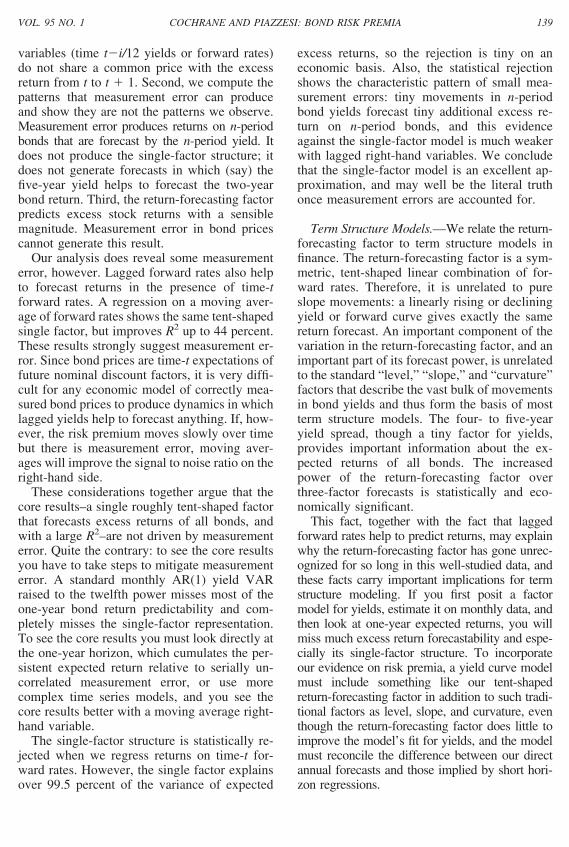
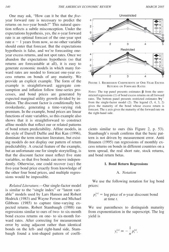
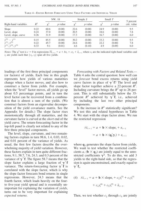
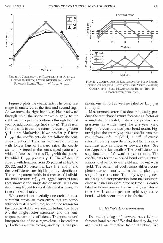
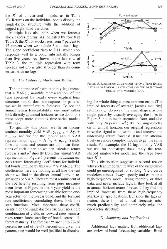
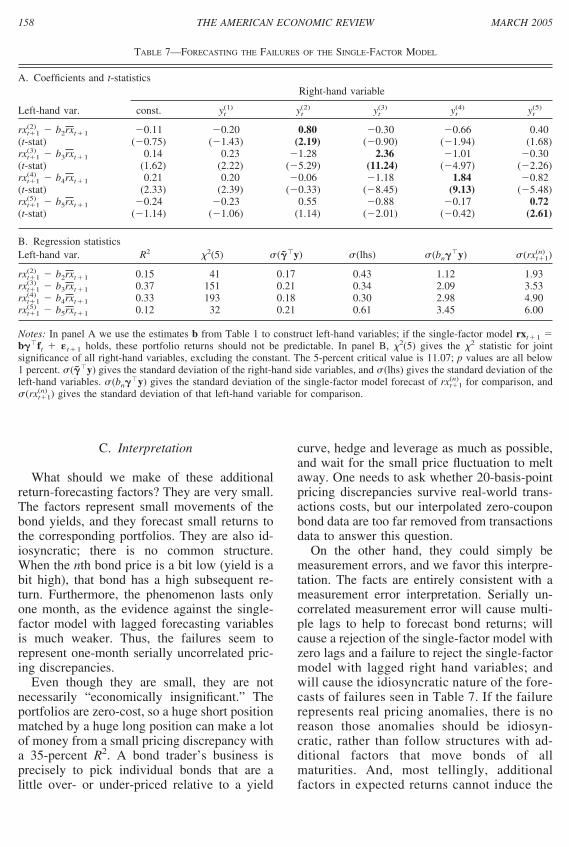
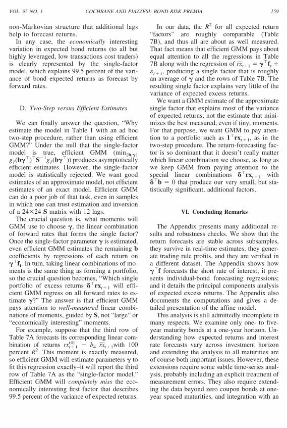