Robust Bond Risk Premia∗

Michael D. Bauer†and James D. Hamilton‡

April 16, 2015Revised: September 28, 2015

Abstract

A consensus has recently emerged that many variables in addition to the level, slope,

and curvature of the yield curve can help predict bond returns. The statistical tests that

led to this conclusion are subject to previously unrecognized size distortions arising from

highly persistent regressors and lagged dependent variables. We revisit the evidence

using tests that are robust to this problem and conclude that the current consensus is

wrong. Only the level and the slope of the yield curve are robust predictors of bond

returns, and there is no convincing evidence of unspanned macro risk.

Keywords: yield curve, spanning, return predictability, robust inference, bootstrap

JEL Classifications: E43, E44, E47

∗The views expressed in this paper are those of the authors and do not necessarily reflect those of othersin the Federal Reserve System. We thank John Cochrane, Graham Elliott, Robin Greenwood, Ulrich Mullerand Glenn Rudebusch for useful suggestions, conference participants at the 7th Annual Volatility InstituteConference at the NYU Stern School of Business and at the NBER 2015 Summer Institute for helpful comments,and Javier Quintero and Simon Riddell for excellent research assistance.†Federal Reserve Bank of San Francisco, michael.bauer@sf.frb.org‡University of California at San Diego, jhamilton@ucsd.edu

1 Introduction

The nominal yield on a 10-year U.S. Treasury bond has been below 2% much of the time since

2011, a level never seen previously. To what extent does this represent unprecedently low

expected interest rates extending through the next decade, and to what extent does it reflect

an unusually low risk premium resulting from a flight to safety and large-scale asset purchases

by central banks that depressed the long-term yield? Finding the answer is a critical input

for monetary policy, investment strategy, and understanding the lasting consequences of the

financial and economic disruptions of 2008.

In principle one can measure the risk premium by the difference between the current

long rate and the expected value of future short rates. But what information should go into

constructing that expectation of future short rates? A powerful argument can be made that

the current yield curve itself should contain most (if not all) information useful for forecasting

future interest rates and bond returns. Investors use information at time t—which we can

summarize by a state vector zt—to forecast future short-term interest rates and determine

bond risk premia. Hence current yields are necessarily a function of zt, reflecting the general

fact that current asset prices incorporate all current information. This suggests that we may

be able to back out the state vector zt from the observed yield curve.1 The “invertibility” or

“spanning” hypothesis states that the current yield curve contains all the information that

is useful for predicting future interest rates or determining risk premia. Notably, under this

hypothesis, the yield curve is first-order Markov.

It has long been recognized that three yield-curve factors, such as the first three principal

components (PCs) of yields, can provide an excellent summary of the information in the entire

yield curve (Litterman and Scheinkman, 1991). While it is clear that these factors, which

are commonly labeled level, slope, and curvature, explain almost all of the cross-sectional

variance of yields, it is less clear whether they completely capture the relevant information for

forecasting future yields and estimating bond risk premia. In this paper we investigate what

we will refer to as the “spanning hypothesis” which holds that all the relevant information

for predicting future yields and returns is spanned by the level, slope and curvature of the

yield curve. This hypothesis differs from the claim that the yield curve follows a first-order

Markov process, as it adds the assumption that only these three yield-curve factors are useful

in forecasting. For example, if higher-order yield-curve factors such as the 4th and 5th PC

are informative about predicting yields and returns, yields would still be Markov, but the

spanning hypothesis, as we define it here, would be violated.

1Specifically, this invertibility requires that (a) we observe at least as many yields as there are state variablesin zt, and (b) there are no knife-edge cancellations or pronounced nonlinearities; see for example Duffee (2013).

1

The spanning hypothesis has two important practical implications for the estimation of

monetary policy expectations and bond risk premia. First, such estimation does not require

any data or models involving macroeconomic series, other asset prices or quantities, volatilities,

or survey expectations, but only the information in interest rates. Second, all that is required

to summarize this information in interest rates is the shape of the current yield curve, measured

by level, slope, and curvature. Notably, the spanning hypothesis is much less restrictive than

the expectations hypothesis, which states that bond risk premia are constant and hence excess

bond returns are not predictable.

However, a number of recent studies have produced evidence that appears to contradict the

spanning hypothesis. Joslin et al. (2014) found that measures of economic growth and inflation

contain substantial predictive power for excess bond returns beyond the information in the

yield curve. Ludvigson and Ng (2009, 2010) documented that factors inferred from a large

set of macro variables help predict bond returns. Cooper and Priestley (2008) found that the

output gap helps predict excess bond returns. Cochrane and Piazzesi (2005) reported evidence

that information in the fourth and fifth PC of yields has predictive power. Greenwood and

Vayanos (2014) found that measures of Treasury bond supply appear to help forecast yields and

returns. Each of these findings suggests that there might be unspanned or hidden information

that is not captured by the level, slope, and curvature of the current yield curve but that is

useful for forecasting.

The key evidence in all these studies comes from predictive regressions for future yields or

excess returns that have two important features. First, the predictive variables are typically

very persistent. Second, some of these predictors summarize the information in the current

yield curve, and therefore are generally correlated with lagged forecast errors, i.e., violate the

condition of strict exogeneity. Although these regressions have a fundamentally different struc-

ture from that considered by Mankiw and Shapiro (1986) and Stambaugh (1999), small-sample

problems that are related to those identified by these researchers turn out to be potentially

important for investigation of the spanning hypothesis. We demonstrate in this paper that

the procedures researchers have been using to deal with problems raised by serial correlation of

the regressors and regression residuals are subject to significant small-sample distortions. We

show for example that the tests employed by Ludvigson and Ng (2009), which are intended to

have a nominal size of five percent, can have a true size of up to 54%. We further demonstrate

that the predictive relations found by all of these researchers exhibit much weaker performance

over subsequent data than they had over the samples originally analyzed by the researchers.

We propose two procedures that researchers could use that would give substantially more

robust small-sample inference. The first is a bootstrap procedure that is designed to test the

2

null hypothesis of interest. We calculate the first three PCs of the observed set of yields and

summarize their dynamics with a VAR fit to the observed PCs. Then we use a parametric

bootstrap to generate artificial samples for the PCs, and construct bootstrapped yields by

multiplying the simulated PCs by the historical loadings of yields on the PCs and adding a

small Gaussian measurement error. Thus by construction no variables other than the PCs are

useful for predicting yields in our generated data. We then fit a separate VAR to the proposed

additional explanatory variables alone, and generate bootstrap samples for the predictors

from this VAR. We can then calculate the properties of any regression statistic under the

null hypothesis that the additional explanatory variables have no predictive power. We find

using this bootstrap procedure that much of the evidence of predictability reported by earlier

researchers in fact fails to pass the usual standards for statistical significance.

A second procedure that we propose for inference in this context is the approach for robust

testing recently suggested by Ibragimov and Muller (2010). We have found this approach

to have excellent size and power properties in settings similar to the ones encountered by

researchers testing for predictive power for interest rates and bond returns. The suggestion

of Ibragimov and Muller (2010) is to split the sample into subsamples, estimate coefficients

separately in each of these, and to perform a simple t-test on the coefficients across subsamples.

Applying this type of test to the predictive regressions for yields and bond returns studied in

the literature, we find that the only robust predictors are the level and the slope of the yield

curve.

We revisit the evidence in the five influential papers cited above, all of which appear to

provide evidence against the null hypothesis of invertibility/spanning. We draw two con-

clusions from our investigation. First, the claims going back to Fama and Bliss (1987) and

Campbell and Shiller (1991) that excess returns can be predicted from the level and slope

of the yield curve remain quite robust. We emphasize that this conclusion is fully consistent

with the Markov property of the yield curve. Second, the newer evidence on the predictive

power of macro variables, higher-order PCs of the yield curve, or other variables, is subject

to more serious econometric problems and appears weaker and much less robust. Overall, we

do not find convincing evidence to reject the hypothesis that the current yield curve, and in

particular three factors summarizing this yield curve, contains all the information necessary

to infer interest rate forecasts and bond risk premia. In other words, the spanning hypothesis

cannot be rejected, and the Markov property of the yield curve seems alive and well.

3

2 Inference about the spanning hypothesis

The evidence against the spanning hypothesis in all of the studies cited in the introduction

comes from regressions of the form

yt+h = β′1x1t + β′2x2t + ut+h, (1)

where the dependent variable yt+h is a yield, a yield curve factor (such as the level of the yield

curve), or a bond return that we wish to predict, x1t and x2t are vectors containing K1 and

K2 predictors, respectively, and ut+h is a forecast error. The predictors x1t contain a constant

and the information in the yield curve, typically captured by the first three PCs of observed

yields, i.e., level, slope, and curvature.2 The null hypothesis of interest is

H0 : β2 = 0,

which says that the relevant predictive information is spanned by the information in the yield

curve and that x2t has no additional predictive power.

The evidence produced in these studies comes in two forms, the first based on simple

descriptive statistics such as how much the R2 of the regression increases when the variables

x2t are added and the second from formal statistical tests of the hypothesis that β2 = 0. In

this section we show how key features of the specification can matter significantly for both

forms of evidence. In Section 2.1 we show how serial correlation in the error term ut and

the proposed predictors x2t can give rise to a large increase in R2 when x2t is added to the

regression even if it is no help in predicting yt+h. In Section 2.2 we note that when x1t is not

strictly exogenous, for example because it includes lagged dependent variables, then when x1t

and x2t are highly persistent processes, conventional heteroskedasticity- and autocorrelation-

consistent tests of whether x2t belongs in the regression can exhibit significant size distortions

in finite samples.

2.1 Implications of serially correlated errors based on first-order

asymptotics

Our first observation is that in regressions in which x1t and x2t are strongly persistent and

the error term is serially correlated—as is always the case with overlapping bond returns—we

should not be surprised to see substantial increases in R2 when x2t is added to the regression

2We will always sign the PCs so that the yield with the longest maturity loads positively on all PCs. As aresult, PC1 and PC2 correspond to what are commonly referred to as “level” and “slope” of the yield curve.

4

even if the true coefficient is zero. It is well known that in small samples serial correlation

in the residuals can increase both the bias as well as the variance of a regression R2 (see for

example Koerts and Abrahamse (1969) and Carrodus and Giles (1992)). To see how much

difference this could make in the current setting, consider the unadjusted R2 defined as

R2 = 1− SSR∑Tt=1(yt+h − yh)2

(2)

where SSR denotes the regression sum of squared residuals. The increase in R2 when x2t is

added to the regression is thus given by

R22 −R2

1 =(SSR1 − SSR2)∑Tt=1(yt+h − yh)2

. (3)

We show in Appendix A that when x1t, x2t, and ut+h are stationary and satisfy standard

regularity conditions, if the null hypothesis is true (β2 = 0) and the extraneous regressors are

uncorrelated with the valid predictors (E(x2tx′1t) = 0), then

T (R22 −R2

1)d→ r′Q−1r/γ (4)

γ = E[yt − E(yt)]2

r ∼ N(0, S), (5)

Q = E(x2tx′2t) (6)

S =∑∞

v=−∞E(ut+hut+h−vx2tx′2,t−v). (7)

Result (4) implies that the difference R22−R2

1 itself converges in probability to zero under the

null hypothesis that x2t does not belong in the regression, meaning that the two regressions

asymptotically should have the same R2.

In a given finite sample, however, R22 is larger than R2

1 by construction, and the above

results give us an indication of how much larger it would be in a given finite sample. If

x2tut+h is serially uncorrelated, then (7) simplifies to S0 = E(u2t+hx2tx′2t). On the other hand,

if x2tut+h is positively serially correlated, then S exceeds S0 by a positive-definite matrix, and

r exhibits more variability across samples. This means R22 − R2

1, being a quadratic form in

a vector with a higher variance, would have both a higher expected value as well as a higher

variance when x2tut+h is serially correlated compared to situations when it is not.

When the dependent variable yt+h is a multi-period bond return, then the error term is

necessarily serially correlated. For example, if yt+h is the h-period excess return on an n-period

5

bond,

yt+h = pn−h,t+h − pnt − hiht, (8)

for pnt the log of the price of a pure discount n-period bond purchased at date t and int =

−pnt/n the corresponding zero-coupon yield, then E(utut−v) 6= 0 for v = 0, . . . , h− 1, due to

the overlapping observations. At the same time, the explanatory variables x2t often are highly

serially correlated, so E(x2tx′2,t−v) 6= 0. Thus even if x2t is completely independent of ut at all

leads and lags, the product will be highly serially correlated,

E(ut+hut+h−vx2tx′2,t−v) = E(utut−v)E(x2tx

′2,t−v) 6= 0.

This serial correlation in x2tut+h would contribute to larger values for R22 − R2

1 on average as

well as to increased variability in R22−R2

1 across samples. In other words, including x2t could

substantially increase the R2 even if H0 is true.3

These results on the asymptotic distribution of R22 − R2

1 could be used to design a test

of H0. However, we show in the next subsection that in small samples additional problems

arise from the persistence of the predictors, with the consequence that the bias and variability

of R22 − R2

1 can be even greater than predicted by (4). For this reason, in this paper we

will rely on an approximation to the small-sample distribution of the statistic R22 − R2

1, and

demonstrate that the dramatic values sometimes reported in the literature are not implausible

under the spanning hypothesis.

Serial correlation of the residuals also affects the sampling distribution of the OLS estimate

of β2. In Appendix A we verify using standard algebra that under the null hypothesis β2 = 0

the OLS estimate b2 can be written as

b2 =(∑T

t=1x2tx′2t

)−1 (∑Tt=1x2tut+h

)(9)

3The same conclusions necessarily also hold for the adjusted R2 defined as

R2i = 1− T − 1

T − kiSSRi∑T

t=1(yt+h − yh)2

for ki the number of coefficients estimated in model i, from which we see that

T (R22 − R2

1) =[T/(T − k1)]SSR1 − [T/(T − k2)]SSR2∑T

t=1(yt+h − yh)2/(T − 1)

which has the same asymptotic distribution as (4). In our small-sample investigations below, we will analyzeeither R2 or R2 as was used in the original study that we revisit.

6

where x2t denotes the sample residuals from OLS regressions of x2t on x1t:

x2t = x2t − ATx1t (10)

AT =(∑T

t=1x2tx′1t

)(∑Tt=1x1tx

′1t

)−1. (11)

If x2t and x1t are stationary and uncorrelated with each other, as the sample size grows,

ATp→ 0 and b2 has the same asymptotic distribution as

b∗2 =(∑T

t=1x2tx′2t

)−1 (∑Tt=1x2tut+h

), (12)

namely √Tb2

d→ N(0, Q−1SQ−1). (13)

with Q and S the matrices defined in (6) and (7). Again we see that positive serial correlation

causes S to exceed the value S0 that would be appropriate for serially uncorrelated residuals.

In other words, serial correlation in the error term increases the sampling variability of the

OLS estimate b2.

The standard approach is to use heteroskedasticity- and autocorrelation-consistent (HAC)

standard errors to try to correct for this, for example, the estimators proposed by Newey and

West (1987) or Andrews (1991). However, in practice different HAC estimators of S can lead

to substantially different empirical conclusions (Muller, 2014). Moreover, we show in the next

subsection that even if the population value of S were known with certainty, it can give a

poor indication of the true small-sample variance. We further demonstrate empirically in the

subsequent sections that this is a serious problem when carrying out inference about interest

rate predictability.

2.2 Small-sample implications of lack of strict exogeneity

A second feature of the studies examined in this paper is that the valid explanatory variables

x1t are correlated with lagged values of the error term. That is, these regressors are only

weakly but not strictly exogenous. This turns out to matter a great deal when x1t and x2t are

highly serially correlated. We noted in the previous subsection that a regression of yt+h on

x1t and x2t can always be thought of as being implemented in several steps, the first of which

involves a regression of x2t on x1t. When these vectors are highly persistent, this auxiliary

regression behaves like a spurious regression in small samples, causing∑x2tx

′2t in (9) to be

significantly smaller than∑x2tx

′2t in (12). When there is correlation between x1t and ut this

7

can cause the usual asymptotic distribution to underestimate significantly the true variability.

In this subsection we demonstrate exactly why this occurs.

But first we note that ours is a different setting from that considered by Mankiw and

Shapiro (1986), Stambaugh (1999) and Campbell and Yogo (2006), who studied tests of the

hypothesis β1 = 0 in a specification of the form

yt+1 = β′1x1t + ut+1 (14)

x1,t+1 = ρ1x1t + ε1,t+1

with x1t a scalar and E(utε1t) 6= 0. Because the regressors x1t are not strictly exogenous,

Stambaugh (1999) showed that the OLS estimate of β1 in (14) will be biased in small samples

and this can significantly affect the small-sample inference when x1t is highly serially correlated

(i.e., when ρ1 is close to one). By contrast, in our study the question is whether the vector

β2 = 0 in (1) is zero. The problem we identify arises even though there is typically no small-

sample bias present in estimates of β2. We will show that for estimates of β2 it is not the

coefficient bias but the inaccuracy of standard errors that distorts the results of conventional

inference. However, as in the case of Stambaugh bias, the small-sample problem in our setting

arises from the fact that the other regressors x1t are not strictly exogenous, and the problem

is most dramatic when x1t and x2t are both highly serially correlated.

2.2.1 Theoretical anlysis using local-to-unity asymptotics

We now demonstrate where the problem arises in the simplest example of our setting. Suppose

that x1t and x2t are scalars that follow independent highly persistent processes,

xi,t+1 = ρixit + εi,t+1 i = 1, 2 (15)

where ρi is close to one. Consider the consequences of OLS estimation of (1) in the special

case where h = 1:

yt+1 = β0 + β1x1t + β2x2t + ut+1. (16)

We assume that (ε1t, ε2t, ut)′ follows a martingale difference sequence with finite fourth mo-

ments and variance matrix

V = E

ε1t

ε2t

ut

[ ε1t ε2t ut

]=

σ21 0 δσ1σu

0 σ22 0

δσ1σu 0 σ2u

. (17)

8

Thus x1t is not strictly exogenous when the correlation δ is nonzero. This is a simple example

to illustrate the problems that can arise when x1t includes variables that are correlated with

lags of the dependent variable. The case δ = 1 corresponds to the case when the explanatory

variable x1t = yt is just the lag of the left-hand variable yt+1 in the regression. Note that for

any δ, x2tut+1 is serially uncorrelated and the standard OLS t-test of β2 = 0 asymptotically

has a N(0, 1) distribution when using the conventional first-order asymptotic approximation.

One device for seeing how the results in a finite sample of some particular size T likely

differ from those predicted by conventional first-order asymptotics is to use a local-to-unity

specification as in Phillips (1988):

xi,t+1 = (1 + ci/T )xit + εi,t+1 i = 1, 2. (18)

For example, if our data come from a sample of size T = 100 when ρi = 0.95, the idea is to

represent this with a value of ci = −5 in (18). The claim is that analyzing the properties as

T → ∞ of a model characterized by (18) with ci = −5 gives a better approximation to the

actual distribution of regression statistics in a sample of size T = 100 and ρi = 0.95 than is

provided by the first-order asymptotics used in the previous subsection which treat ρi as a

constant when T →∞; see for example Chan (1988) and Nabeya and Sørensen (1994).

The local-to-unity asymptotics turn out to be described by Ornstein-Uhlenbeck processes.

For example

T−2∑T

t=1(xit − xi)2 ⇒ σ2

i

∫ 1

0

[Jµci(λ)]2dλ

where ⇒ denotes weak convergence as T →∞ and

Jci(λ) = ci

∫ λ

0

eci(λ−s)Wi(s)ds+Wi(λ) i = 1, 2

Jµci(λ) = Jci(λ)−∫ 1

0

Jci(s)ds i = 1, 2

with W1(λ) and W2(λ) denoting independent standard Brownian motion. When ci = 0, (18)

becomes a random walk and the local-to-unity asymptotics simplify to the standard unit-root

asymptotics involving functionals of Brownian motion as a special case: J0(λ) = W (λ).

We show in Appendix B that under local-to-unity asymptotics the coefficient from a re-

gression of x2t on x1t has the following limiting distribution:

AT =

∑(x1t − x1)(x2t − x2)∑

(x1t − x1)2⇒

σ2∫ 1

0Jµc1(λ)Jµc2(λ)dλ

σ1∫ 1

0[Jµc1(λ)]2dλ

= (σ2/σ1)A. (19)

9

Thus whereas under first-order asymptotics the influence of AT vanishes as the sample size

grows, using the local-to-unity approximation AT behaves in a similar way to the coefficient

in a spurious regression; AT does not converge to zero—the true correlation between x1t and

x2t in this setting—but to a random variable that takes on a different value in each sample.

Because the regression coefficient on x2t in the original regression (1) can be written as in (9)

in terms of the residuals of this near-spurious regression, the result is that in small samples

with persistent regressors the t-statistic for β2 = 0 has a very different distribution from that

predicted using first-order asymptotics. We demonstrate in Appendix B that this t-statistic

has a local-to-unity asymptotic distribution under the null hypothesis that is given by

b2

{s2/∑x22t}

1/2⇒ δZ1 +

√1− δ2Z0 (20)

Z1 =

∫ 1

0Kc1,c2(λ)dW1(λ){∫ 1

0[Kc1,c2(λ)]2dλ

}1/2(21)

Z0 =

∫ 1

0Kc1,c2(λ)dW0(λ){∫ 1

0[Kc1,c2(λ)]2dλ

}1/2(22)

Kc1,c2(λ) = Jµc2(λ)− AJµc1(λ)

for s2 = (T − 3)−1∑

(yt+1 − b0 − b1x1t − b2x2t)2 and Wi(λ) independent standard Brownian

processes for i = 0, 1, 2. Conditional on the realizations of W1(.) and W2(.), the term Z0 will

be recognized as a standard Normal variable, and therefore Z0 has an unconditional N(0, 1)

distribution as well.4 In other words, if x1t is strictly exogenous (δ = 0) then the OLS t-test

of β2 = 0 will be valid in small samples even with highly persistent regressors. By contrast,

the term dW1(λ) in the numerator of (21) is not independent of the denominator and this

gives Z1 a nonstandard distribution. In particular, Appendix B establishes that V ar(Z1) > 1.

Moreover Z1 and Z0 are uncorrelated with each other.5 Therefore the t-statistic in (20) in

general has a non-standard distribution with variance δ2Var(Z1) + (1 − δ2)1 > 1 which is

monotonically increasing in |δ|. This leads us to our key result: Whenever x1t is correlated

4The intuition is that for v0,t+1 ∼ i.i.d. N(0, 1) and K = {Kt}Tt=1 any sequence of random variables

that is independent of v0,∑Tt=1Ktv0,t+1 has a distribution conditional on K that is N(0,

∑Tt=1K

2t ) and∑T

t=1Ktv0,t+1/√∑T

t=1K2t ∼ N(0, 1). Multiplying by the density of K and integrating over K gives the

identical unconditional distribution, namely N(0, 1). For a more formal discussion in the current setting, seeHamilton (1994, pp. 602-607).

5The easiest way to see this is to note that conditional on W1(.) and W2(.) the product has expectationzero, so the unconditional expected product is zero as well.

10

with ut (δ 6= 0) and x1t and x2t are highly persistent, in small samples the t-test of β2 = 0

will reject too often when H0 is true. The intuition for this result is that the OLS estimate

of β2 in (1), b2, can be obtained in three steps: (i) regress x2t on x1t, (ii) regress yt+h on x1t,

and (iii) regress the residuals from (ii) on the residuals of (i). The small-sample properties of

the first regression are very different when x1t and x2t are highly persistent. When x1t is not

strictly exogenous this can end up mattering a great deal for the small-sample distribution of

b2.

2.2.2 Simulation evidence

We now examine the implications of the theory developed above in a simulation study. We

generate values for x1t and x2t using (15), with ε1t and ε2t serially independent Gaussian

random variables with unit variance and covariance equal to γ.6 We then calculate

yt+1 = ρ1x1t + ut+1, ut = δε1t +√

1− δ2vt,

where vt is an i.i.d. standard normal random variable. This implies that in the predictive

equation (16) the true parameters are β0 = β2 = 0 and β1 = ρ1, and that the correlation

between ut and ε1t is δ. Note that for δ = 1 this corresponds to a model with a lagged

dependent variable (yt = x1t), whereas for δ = 0 both predictors are strictly exogenous as ut

is independent of both both ε1t and ε2t. We first set γ = 0 as in our theory above, so that

the variance matrix V is given by equation (17) with σ1, σ2, and σu equal to one, and x2t is

strictly exogenous. We investigate the effects of varying δ, the persistence of the predictors

(ρ1 = ρ2 = ρ), and the sample size T . We simulate 50,000 artificial data samples, and in

each sample we estimate the regression in equation (16). Since our interest is in the inference

about β2 we use this simulation design to study the small-sample behavior of the t-statistic

(calculated using OLS standard errors) for the test of H0 : β2 = 0.

In addition to the small-sample distribution of the t-statistic we also study its asymptotic

distribution given in equation (20). While this is a non-standard distribution, we can draw

from it using Monte Carlo simulation: for given values of c1 and c2, we simulate samples of size

T from near-integrated processes and approximating the integrals using Rieman sums—see,

for example, Chan (1988), Stock (1991), and Stock (1994). The literature suggests that such

a Monte Carlo approach yields accurate approximations to the limiting distribution even for

moderate sample sizes (Stock, 1991, uses T = 500). We will use T = 1000 and generate 50,000

6We start the simulations at x1,0 = x2,0 = 0, following standard practice of making all inference conditionalon date 0 magnitudes.

11

Monte Carlo replications with c1 = c2 = T (ρ − 1) to calculate the predicted outcome for a

sample of size T with serial dependence ρ.

Table 1 reports the performance of the t-test of H0 with a nominal size of five percent. It

shows the true size of this test, i.e., the frequency of rejections of H0, according to both the

small-sample distribution from our simulations and the asymptotic distribution in equation

(20). We use critical values from a Student t-distribution with T − 3 degrees of freedom.

We find that in this setting the local-to-unity asymptotic distribution provides an excellent

approximation to the exact small-sample distributions, as both indicate a very similar test

size across parameter configurations and sample sizes. In general, size distortions are present

when strict exogeneity is violated (δ 6= 0), and they can be very substantial, with a true size of

up to 17 percent even in this simple setting. This means that in those cases, the t-test would

reject the null more than three times as often as it should. Results for δ < 0, which we do not

report, exactly parallel the reported results for δ > 0 because only the absolute magnitude of

δ matters for the distribution of the t-statistic. When δ 6= 0, the size of the t-test increases

with the persistence of the regressors. Table 1 also shows the dependence of the size distortion

on the sample size. To visualize this, Figure 1 plots the empirical size of the t-test for the

case with δ = 1 for different sample sizes from T = 50 to T = 1000.7 When ρ < 1, the size

distortions decrease with the sample size—for example for ρ = 0.99 the size decreases from

15 percent to about 9 percent. In contrast, when ρ = 1 the size distortions are not affected

by the sample size, as indeed in this case the non-Normal distribution corresponding to (20)

with ci = 0 governs the distribution for arbitrarily large T . Figure 1 also shows that our local-

to-unity results give very accurate approximations to the true small-sample distributions, in

particular for sample sizes larger than about T = 200.

To understand better why conventional t-tests go so wrong in this setting, we use simu-

lations to study the respective roles of bias in the coefficient estimates and of inaccuracy of

the OLS standard errors for estimation of β1 and β2. Table 2 shows results for three different

simulation settings, in all of which T = 100, ρ = 0.99, and x1t is correlated with past forecast

errors (δ 6= 0). In the first two settings, the correlation between the regressors is zero (γ = 0),

and δ is either equal to one or 0.8. In the third setting, we investigate the effects of non-zero

correlation between the predictors by setting δ = 0.8 and γ = 0.8. Note that in this setting,

x2t is not strictly exogenous, as the correlation between ut and ε2t is γδ.8 The results show

7The lines in Figure 1 are based on 500,000 simulated samples in each case.8A correlation between ut and ε2t of γδ is the natural implication of a model in which only x1t contains

information useful for predicting yt. If instead we insisted on E(utε2t) = 0 while γ 6= 0 (or, more generally,if E(utε2t) 6= γδ) then E(yt|x1t, x1,t−1, x2t, x2,t−1) 6= E(yt|x1t, x1,t−1) meaning that in effect yt would dependon both x1t and x2t.

12

that in all three simulation settings b1 is downward biased and b2 is unbiased.9 Evidently the

problem with hypothesis tests of β2 = 0 does not arise from Stambaugh bias as traditionally

understood. Instead of coefficient bias, the reason for the size distortions of these tests is

the fact that the OLS standard errors substantially underestimate the sampling variability

of both b1 and b2. This is evident from comparing the standard deviation of the coefficient

estimates across simulations—the true small-sample standard error—and the average OLS

standard errors. The difference, which we term “standard error bias,” can be substantial: in

the first setting, the standard errors for both b1 and b2 are on average about 30% too low.

We also consider tests of the (true) hypothesis β1 = 0.99, and note that for this test both

coefficient bias (i.e., Stambaugh bias) and standard error bias play a role. In sum, both our

econometric theory and our small-sample simulations have shown that lack of strict exogeneity

not only causes Stambaugh bias for some predictors, but it also causes standard error bias

for all predictors, which can make inference unreliable even for those predictors that are not

affected by Stambaugh bias.

We have also calculated (though results are not reported here) the increase in R2 when

x2t is added to the regression, and find that lack of strict exogeneity of x1t can also make the

problem identified in Section 2.1 using first-order asymptotics even more severe.

2.2.3 Relevance for applied work

We have demonstrated that with persistent predictors, the lack of strict exogeneity of a sub-

set of the predictors can have significant consequences for the small-sample inference on the

remaining predictors. This result has broad relevance, as it arises in many situations that

are commonly encountered in time series analysis. These include lagged-dependent-variable

(LDV) models and tests for Granger causality. The practical implication is that unless the

sample size is large and the regressors not too persistent, the conventional hypothesis tests

used in these situations are likely to be misleading. Importantly, HAC standard errors do

not help, because in such settings they cannot accurately capture the uncertainty surrounding

the coefficient estimators. It appears that this small-sample problem with LDV models and

Granger causality tests has not previously been noticed.

Our result is particularly relevant for tests of the spanning hypothesis. In all of the

empirical studies that we consider in this paper, the predictors in x1t are correlated with

past error terms. The reason is that they correspond to information in current yields, and the

dependent variable is either a future bond return or the future level of the yield curve. The

9Stambaugh (1999) focused on δ < 0 in which case estimates for β1 are biased upward, but given our focuson β2 the sign of δ is irrelevant.

13

resulting lack of strict exogeneity is a separate issue from serial correlation in the residuals,

which necessarily arises for overlapping returns. Both issues become particularly serious when

the predictors are persistent and when the sample sizes are small, which is the case in applied

work on interest rates.10 In Table 3 we report the estimated autocorrelation coefficients for the

predictors used in the published studies that we investigate in the following sections. Clearly,

many of the predictors considered in the literature are highly persistent, and we need to

be particularly concerned about the aforementioned small-sample issues. Adding extraneous

regressors that in reality contribute nothing to prediction may lead to an artificially large

increase in the R2 and inflated values for t- and F -statistics. We now describe a methodology

that will allow us to quantify just how important this issue is in a given data set and to obtain

more reliable inference that accounts for these small sample problems.

2.3 A bootstrap design for investigating the spanning hypothesis

The above analysis suggests that it is of paramount importance to base inference on the small-

sample distributions of the relevant test statistics. We propose to do so using a parametric

bootstrap under the null hypothesis. While some studies (Bekaert et al., 1997; Cochrane and

Piazzesi, 2005; Ludvigson and Ng, 2009; Greenwood and Vayanos, 2014) use the bootstrap in

a similar context, they typically do so by generating samples under the absence of predictabil-

ity, which can be used to test the expectations hypothesis but not the spanning hypothesis.

Cochrane and Piazzesi (2005) and Ludvigson and Ng (2009, 2010) also calculated bootstrap

confidence intervals under the alternative hypothesis, which in principle gives some indication

of the small-sample significance of the coefficients on x2t. However, bootstrapping under the

relevant null hypothesis is much to be preferred. It allows us to calculate the small-sample size

of conventional tests and should lead to better numerical accuracy and more powerful tests

(Hall and Wilson, 1991; Horowitz, 2001). Our paper is the first to propose a bootstrap to test

the spanning hypothesis H0 : β2 = 0 by generating bootstrapped samples under the null.

Our bootstrap design is as follows: First, we calculate the first three PCs of observed yields

which we denote

x1t = (PC1t, PC2t, PC3t)′,

along with the weighting vector wn for the bond yield with maturity n:

int = w′nx1t + vnt.

10Reliable interest rate data are only available since about the 1960s, which leads to situations with about40-50 years of monthly data. Going to higher frequencies—such as weekly or daily—does not increase theeffective sample sizes, since it typically increases the persistence of the series and introduces additional noise.

14

That is, x1t = W it, where it = (in1t, . . . , inJ t)′ is a J-vector with observed yields at t, and

W = (wn1 , . . . , wnJ)′ is the 3× J matrix with rows equal to the first three eigenvectors of the

variance matrix of it. We use normalized eigenvectors so that WW ′ = I3.11 Fitted yields can

be obtained using ıt = W ′x1t. Three factors generally fit the cross section of yields very well,

with fitting errors vnt (pooled across maturities) that have a standard deviation of only a few

basis points.12

Then we estimate by OLS a VAR(1) for x1t:

x1t = φ0 + φ1x1,t−1 + e1t t = 1, . . . , T. (23)

This time-series specification for x1t completes our simple factor model for the yield curve.

Though this model does not impose absence of arbitrage, it captures both the dynamic evolu-

tion and the cross-sectional dependence of yields. Studies that have documented that such a

simple factor model fits and forecasts the yield curve well include Duffee (2011) and Hamilton

and Wu (2014).

Next we generate 5000 artificial yield data samples from this model, each with length T

equal to the original sample length. We first iterate13 on

x∗1τ = φ0 + φ1x∗1,τ−1 + e∗1τ

where e∗1τ denotes bootstrap residuals. Then we obtain the artificial yields using

i∗nτ = w′nx∗1τ + v∗nτ (24)

for v∗nτ ∼ N(0, σ2v). The standard deviation of the measurement errors, σv, is set to the sample

standard deviation of the fitting errors vnt. We thus have generated an artificial sample of

yields i∗nτ which by construction only three factors (the elements of x∗1τ ) have any power to

predict, but whose covariance and dynamics are similar to those of the observed data int.

Notably, our bootstrapped yields are first-order Markov—under our bootstrap the current

yield curve contains all the information necessary to forecast future yields.

11We choose the eigenvectors so that the elements in the last column of W are positive—see also footnote 2.12For example, in the case study of Joslin et al. (2014) in Section 3, the standard deviation is 6.5 basis

points.13We start the recursion with a draw from the unconditional distribution implied by the estimated VAR for

x1t.

15

We likewise fit a VAR(1) to the observed data for the proposed predictors x2t,

x2t = α0 + α1x2,t−1 + e2t, (25)

from which we then bootstrap 5000 artificial samples x∗2τ in a similar fashion as for x∗1τ . The

bootstrap residuals (e′∗1τ , e′∗2τ ) are drawn from the joint empirical distribution of (e′1t, e

′2t).

14

Using the bootstrapped samples of predictors and yields, we can then investigate the

properties of any proposed test statistic involving y∗τ+h, x∗1τ , and x∗2τ in a sample for which

the dynamic serial correlation of yields and explanatory variables are similar to those in the

actual data but in which by construction the null hypothesis is true that x∗2τ has no predictive

power for future yields and bond returns.15 In particular, under our bootstrap there are no

unspanned macro risks.

How can we use our bootstrap procedure to test the spanning hypothesis? As an example,

consider a t-test for significance of a parameter in β2. Denote the t-statistic in the data by

t and the corresponding t-statistic in bootstrap sample i as t∗i . We calculate the bootstrap

p-value as the fraction of samples in which |t∗i | > |t|, and would reject the null if this is less

than, say, five percent. In addition, we can estimate the true size of a conventional t-test as

the fraction of samples in which |t∗i | exceeds the usual asymptotic critical value.

Unfortunately, the distribution of the test statistics depends on ρ1 and ρ2 through local-

to-unity parameters like c1 and c2 that cannot be consistently estimated. For this reason,

our bootstrap procedure delivers a test of H0 that does not have a size of five percent. If the

data had actually been generated by VARs with parameters φ1 and α1, then our procedure

would have the correct size by construction. The problem is that we only have estimates of

the true parameters that determine the persistence of the predictors, and the test statistics

are not asymptotically pivotal as their distribution depends on c1 and c2.16

We can use the Monte Carlo simulations in Section 2.2.2 to calculate what the size of our

14We also experimented with a Monte Carlo design in which e∗1τ was drawn from a Student-t dynamicconditional correlation GARCH model (Engle, 2002) fit to the residuals e1t with similar results to thoseobtained using independently resampled e1t and e2t.

15For example, if yt+h is an h-period excess return as in equation (8) then in our bootstrap

y∗τ+h = ni∗nτ − hi∗hτ − (n− h)i∗n−h,τ+h

= n(w′nx∗1τ + v∗nτ )− h(w′hx

∗1τ + v∗hτ )− (n− h)(w′n−hx

∗1,τ+h + v∗n−h,τ+h)

= n(w′nx∗1τ + v∗nτ )− h(w′hx

∗1τ + v∗hτ )− (n− h)[w′n−h(kh + e∗1,τ+h + φ1e

∗1,τ+h−1 + · · ·

+ φh−11 e∗1,τ+1 + φh1x∗1τ ) + v∗n−h,τ+h]

which replicates the date t predictable component and the MA(h−1) serial correlation structure of the holdingreturns that is both seen in the data and predicted under the spanning hypothesis.

16This problem is well known in the bootstrap literature, see for example Horowitz (2001).

16

bootstrap procedure would be if applied to a specified parametric model. In each sample i

simulated from a known parametric model, we can: (i) calculate the usual t-statistic (denoted

ti) for testing the null hypothesis that β2 = 0; (ii) estimate the autoregressive models for the

predictors by using OLS on that sample; (iii) generate a single bootstrap simulation using these

estimated autoregressive coefficients; (iv) estimate the predictive regression on the bootstrap

simulation;17 (v) calculate the t-test of β2 = 0 on this bootstrap predictive regression, denoted

t∗i . We generate 5,000 samples from the maintained model, repeating steps (i)-(v), and then

calculate the value c such that |t∗i | > c in 5% of the samples. Our bootstrap procedure

amounts to the recommendation of rejecting H0 if |ti| > c, and we can calculate from the

above simulation the fraction of samples in which this occurs. This number tells us the

true size if we were to apply our bootstrap procedure to the chosen parametric model. This

number is reported in the second-to-last row of Table 2. We find in these settings that our

bootstrap has a size above but fairly close to five percent. The size distortion is always smaller

for our bootstrap than for the conventional t-test.

We will repeat the above procedure to estimate the size of our bootstrap test in each

of our empirical applications, taking a model whose true coefficients are those of the VAR

estimated in the sample as if it were the known parametric model, and estimating VAR’s from

data generated using those coefficients. To foreshadow those results, we will find that the

size is typically quite close to or slightly above five percent. The implication is that if our

bootstrap procedure fails to reject the spanning hypothesis at a nominal five-percent level, we

can appropriately conclude that the evidence against the spanning hypothesis in the original

data is not persuasive.

A separate but related issue is that least squares typically underestimates the autocor-

relation of highly persistent processes due to small-sample bias (Kendall, 1954; Pope, 1990).

Therefore the VAR we use in our bootstrap would typically be less persistent than the true

data-generating process. For this reason, we might expect the bootstrap procedure to be

slightly oversized.18 One way to deal with this issue is to generate samples not from the OLS

estimates φ1 and α1 but instead use bias-corrected VAR estimates obtained with the bootstrap

adopted by Kilian (1998). We refer to this below as the “bias-corrected bootstrap.” We have

found in Monte Carlo experiments that even the bias-corrected bootstrap tends to be slightly

oversized, though the distortion is somewhat smaller than that for the regular bootstrap.

17In this simple Monte Carlo setting, we bootstrap the dependent variable as y∗τ = φ1x∗1,τ−1 +u∗τ where u∗τ is

resampled from the residuals in a regression of yt on x1,t−1, and is jointly drawn with ε∗1τ and ε∗2τ to maintainthe same correlation as in the data. By contrast, in all our empirical analysis the bootstrapped dependentvariable is obtained from (24) and the definition of yt+h (for example, equation (8)).

18A test that would have size five percent if the serial correlation was given by ρ1 = 0.97 would have sizegreater than five percent if the true serial correlation is ρ1 = 0.99.

17

2.4 An alternative robust test for predictability

There is of course a very large literature addressing the problem of HAC inference. This

literature is concerned with accurately estimating the matrix S in (7) but does not address

what we have identified as the key issue, which is the small-sample difference between the

statistics in (9) and (12). We have looked at a number of alternative approaches in terms of

how well they perform in our bootstrap experiments. We found that the most reliable existing

test appears to be the one suggested by Ibragimov and Muller (2010), who proposed a novel

method for testing a hypothesis about a scalar coefficient. The original dataset is divided into

q subsamples and the statistic is estimated separately over each subsample. If these estimates

across subsamples are approximately independent and Gaussian, then a standard t-test with q

degrees of freedom can be carried out to test hypotheses about the parameter. Muller (2014)

provided evidence that this test has excellent size and power properties in regression settings

where standard HAC inference is seriously distorted. Our simulation results, to be discussed

below, show that this test also performs very well in the specific settings that we consider

in this paper, namely inference about predictive power of certain variables for future interest

rates and excess bond returns. Throughout this paper, we report two sets of results for the

Ibragimov-Muller (IM) test, setting the number of subsamples q equal to either 8 and 16 (as

in Muller, 2014). A notable feature of the IM test is that it allows us to carry out inference

that is robust not only with respect to serial correlation but also with respect to parameter

instability across subsamples, as we will discuss Section 5.

We use the same Monte Carlo simulation as before to estimate the size of the IM test in

the simple setting with two scalar predictors. The results are shown in the last row of Table

2. The IM test has close to nominal size in all three settings. The reason is that the IM test

is based on more accurate estimates of the sampling variability of the test statistic by using

variation across subsamples. In this way, it solves the problem of standard error bias that

conventional t-tests are faced with. Note, however, that coefficient bias would be a problem

for the IM test, because it splits the (already small) sample into even smaller samples, which

would magnify the small-sample coefficient bias. It is therefore important to assess whether

the conditions are met for the IM test to work well in practice, which we will do below in our

empirical applications. It will turn out that in our applications the IM test should perform

very well.

18

3 Predicting yields using economic growth and inflation

In this section we examine some of the evidence reported by Joslin et al. (2014) (henceforth

JPS) that macro variables may help predict bond yields.

3.1 Excess bond returns

We begin with some of the most dramatic findings reported by JPS, which come from predictive

regressions as in equation (1) where yt+h is an excess bond return for a one-year holding

period (h = 12), x1t is a vector consisting of a constant and the first three PCs of yields, and

x2t a vector consisting measures of economic growth and inflation. JPS found that for the

ten-year bond, the adjusted R2 of regression (1) when x2t is excluded is only 0.20 when the

regression was estimated over the period 1985:1-2007:12. But when they added x2t, consisting

of economic growth measured by a three-month moving average of the Chicago Fed National

Activity Index (GRO) and inflation measured by one-year CPI inflation expectations from

the Blue Chip Financial Forecasts (INF ), the R2 increased to 0.37. For the two-year bond,

the change is even more striking, with R2 increasing from 0.14 without the macro variables

to 0.48 when they are included. JPS interpreted these adjusted R2 as strong evidence that

macroeconomic variables have predictive power for excess bond returns beyond the information

in the yield curve itself, and concluded from this evidence that “macroeconomic risks are

unspanned by bond yields” (p. 1203).

However, there are some warning flags for these predictive regressions, which we report in

Table 3. First, the predictors in x2t are very persistent. The first-order sample autocorrelations

for GRO and INF are 0.91 and 0.99, respectively. The yield PCs in x1t, in particular the level

and slope, are of course highly persistent as well, which is a common feature of interest rate

data. Second, to assess strict exogeneity of the predictors we report estimated values for δ, the

correlation between innovations to the predictors, ε1t and ε2t, and the lagged prediction error,

ut.19 The innovations are obtained from the estimated VAR models for x1t and x2t, and the

prediction error is calculated from least squares estimates of equation (1) for yt+h the average

excess bond return for two- through ten-year maturities. For the first PC of yields, the level of

the yield curve, strict exogeneity is strongly violated, as the absolute value of δ is substantial.

Its sizable negative value is due to the mechanical relationship between bond returns and the

level of the yield curve: a positive innovation to PC1 at t raises all yields and mechanically

lowers bond returns from t − h to t. Hence such a violation of strict exogeneity will always

19While in our theory in Section 2.2 δ was the correlation of the (scalar) innovation of x1t with past predictionerrors, here we calculate it for all predictors in x1t and x2t.

19

be present in predictive regressions for bond returns that include the current level of the yield

curve. In light of our results in Section 2 these warning flags suggest that small-sample issues

are present, and we will use the bootstrap to address them.

Table 4 shows R2 of predictive regressions for the excess bond returns on the two- and

ten-year bond, and for the average excess return across maturities. The first three columns

are for the same data set as was used by JPS.20 The first row in each panel reports the actual

R2, and for the excess returns on the 2-year and 10-year bonds essentially replicates the results

in JPS.21 The entry R21 gives the adjusted R2 for the regression with only x1t as predictors,

and R22 corresponds to the case when x2t is added to the regression. The second row reports

the mean R2 across 5000 replications of the bootstrap described in Section 2.3, that is, the

average value we would expect to see for these statistics in a sample of the size used by JPS in

which x2t in fact has no true ability to predict yt+h but whose serial correlation properties are

similar to those of the observed data. The third row gives 95% confidence intervals, calculated

from the bootstrap distribution of the test statistics.

For all predictive regressions, the variability of the adjusted R2 is very high. Values for R22

up to about 63% would not be uncommon, as indicated by the bootstrap confidence intervals.

Most notably, adding the regressors x2t often substantially increases the adjusted R2, by

up to 23 percentage points or more, although x2t has no predictive power in population by

construction. For the ten-year bond, JPS report an increase of 17 percentage points when

adding macro variables, but our results show that this increase is in fact not statistically

significant at conventional significance levels. For the two-year bond, the increase in R2 of 35

percentage points is statistically significant. However, the two-year bond seems to be special

among the yields one could look at. When we look for example at the average excess return

across all maturities, our bootstrap finds no evidence that x2t has predictive power beyond

the information in the yield curve, as reported in the last panel of Table 4.

Since the persistence of x2t is high, it may be important to adjust for small-sample bias

in the VAR estimates. For this reason we also carried out the bias-corrected (BC) bootstrap.

The expected values and 95% confidence intervals are reported in the bottom two rows of

each panel of Table 4. As expected, more serial correlation in the generated data (due to

20Their yield data set ends in 2008, with the last observation in their regression corresponding to the excessbond return from 2007:12 to 2008:12.

21The yield data set of JPS includes the six-month and the one- through ten-year Treasury yields. Aftercalculating annual returns for the two- to ten-year bonds, JPS discarded the six, eight, and nine-year yieldsbefore fitting PCs and their term structure models. Here, we need the fitted nine-year yield to construct thereturn on the ten-year bond, so we keep all 11 yield maturities. While our PCs are therefore slightly differentthan those in JPS, the only noticeable difference is that our adjusted R2 in the regressions for the two-yearbond with yield PCs and macro variables is 0.49 instead of their 0.48.

20

the bias correction) increases the mean and the variability of the adjusted R2 and of their

difference. In particular, while the difference R22 − R2

1 for the average excess return regression

was marginally significant at the 10-percent level for the simple bootstrap, it is insignificant

at this level for the BC bootstrap.

The right half of Table 4 updates the analysis to include an additional 7 years of data.

As expected under the spanning hypothesis, the value of R22 that is observed in the data

falls significantly when new data are added. And although the bootstrap 95% confidence

intervals for R21− R2

2 are somewhat tighter with the longer data set, the conclusion that there

is no statistically significant evidence of added predictability provided by x2t is even more

compelling. For all bond maturities, the increases in adjusted R2 from adding macro variables

as predictors for excess returns lie comfortably inside the bootstrap confidence intervals.

3.2 Predicting the level of the yield curve

JPS went on to estimate yield-curve models in which it is assumed that the macro factors x2t

directly help predict the PCs x1t. Their Table 3 reports the model-implied estimates for the

VAR for xt = (x′1t, x′2t)′, which indicate that the coefficients on x2t are highly significant. Here

we reassess this evidence, focusing on the first equation of this VAR, which predicts the level

(first PC) of the yield curve. This regression is the crucial forecasting equation, since forecasts

of any yield are dominated by the forecast for the first PC. The estimated coefficients from

this regression are reported in the first row of Table 5. Although we simply use least squares

while JPS use a no-arbitrage model with overidentifying restrictions, our estimates are similar

to the estimates reported in the first row of JPS Table 3.22

The standard errors in JPS’ original Table 3 incorporate the restrictions implied by the

structural model but make no allowance for possible serial correlation of the product xtut+1.

One popular approach to guard against this possibility is to use the HAC standard errors

and test statistics proposed by Newey and West (1987). In the second row of Table 5 we

report the resulting t-statistic for each coefficient along with the Wald test of the hypothesis

β2 = 0, calculated using Newey-West standard errors with four lags (based on the automatic

lag selection of Newey and West, 1994). The third row reports asymptotic p-values for these

statistics.

We then employ our bootstrap to carry out tests of the spanning hypothesis that account

for the small-sample issues described in Section 2. Again, we use both a simple bootstrap

based on OLS estimates of the VAR parameters, as well as a bias-corrected (BC) bootstrap.

22To make our estimates comparable to those of JPS, we rescale our PCs in the same way (see footnote 19of JPS).

21

For each, we report five-percent critical values for the t- and Wald statistics, calculated as

the 95th percentiles of the bootstrap distribution, as well as bootstrap p-values, i.e., the

frequency of bootstrap replications in which the bootstrapped test statistics are at least as

large as in the data. Using the simple bootstrap, the coefficient on GRO is only marginally

significant (p = 4.8%) while INF is insignificant. Using the BC bootstrap, both coefficients

are insignificant at the five-percent level, in contrast to what is indicated by conventional

t-tests. While the bootstrap Wald tests do reject the spanning hypothesis at the five-percent

significance level, they do not reject at the one-percent level, again in stark contrast to the

conventional tests.

We also report in Table 5 the p-values for the IM test of the individual significance of the

coefficients. The level of the yield curve (PC1) is a strongly significant predictor, with p-values

below 0.1% for both IM tests. This will turn out to be a consistent finding in all the data

sets that we will look at—the level or slope of the yield curve appear to be robust predictors

of future interest rates and bond risk premia, consistent with an old literature going back to

Fama and Bliss (1987) and Campbell and Shiller (1991).23 By contrast, the coefficients on

GRO and INF are not statistically significant at conventional significance levels based on the

IM test.

We then use the bootstrap to calculate the properties of the different tests for data with

serial correlation properties similar to those observed in the sample. In particular, we estimate

the true size of the HAC, bootstrap, and IM tests with nominal size of five percent. The results,

which are shown in the last four rows of the top panel of Table 5, reveal that the true size of

the conventional HAC tests is 10-18% instead of the presumed five percent.24 The bootstrap

and the IM tests, in contrast, have a size that is estimated to be very close to five percent,

eliminating almost all of the size distortions of the more conventional tests.

When we add more data to the sample, we again find that the statistical evidence of pre-

dictability declines substantially, as seen in the second panel of Table 5. When the data set is

extended through 2013, the HAC test statistics are only marginally significant or insignificant,

even if interpreted assuming the usual asymptotics. Using the bootstrap to take into account

the small-sample size distortions of such tests, these test statistics are far from significant.

Regarding the results for the IM test, we also find in this extended sample that the level is

an important predictor of its future value, whereas the coefficients on the macro variables are

insignificant.

We conclude that the evidence in JPS on the predictive power of macro variables for yields

23The low p-values are also consistent with the conclusion from our unreported Monte Carlo investigationthat IM has good power to reject a false null hypothesis.

24Using the BC bootstrap gives an even higher estimate of the true size of the HAC Wald test, about 23%.

22

and bond returns is not altogether convincing. Notwithstanding, JPS noted that theirs is only

one of several papers claiming to have found such evidence. We turn in the next section to

another influential study.

4 Predicting yields using factors of large macro data

sets

Ludvigson and Ng (2009, 2010) found that factors extracted from a large macroeconomic

data set are helpful in predicting excess bond returns, above and beyond the information

contained in the yield curve, adding further evidence for the claim of unspanned macro risks

and against the hypothesis of invertibility. Here we revisit this evidence, focusing on the

results in Ludvigson and Ng (2010) (henceforth LN).

LN started with a panel data set of 131 macro variables observed over 1964:1-2007:12 and

extracted eight macro factors using the method of principal components. These factors, which

we will denote by F1 through F8, were then related to future one-year excess returns on two-

through five-year Treasury bonds. The authors carried out an extensive specification search

in which they considered many different combinations of the factors along with squared and

cubic terms. They also included in their specification search the bond-pricing factor proposed

by Cochrane and Piazzesi (2005), which is the linear combination of forward rates that best

predicts the average excess return across maturities, and which we denote here by CP. LN’s

conclusion was that macro factors appear to help predict excess returns, even when controlling

for the CP factor. This conclusion is mostly based on comparisons of adjusted R2 in regressions

with and without the macro factors and on HAC inference using Newey-West standard errors.

4.1 Robust inference about coefficients on macro factors

One feature of LN’s design obscures the evidence relevant for the null hypothesis that is

the focus of our paper. Their null hypothesis is that the CP factor alone provides all the

information necessary to predict bond yields, whereas our null hypothesis of interest is that

the 3 variables (PC1, PC2, PC3) contain all the necessary information. Their regressions in

which CP alone is used to summarize the information in the yield curve could not be used to

test our null hypothesis. For this reason, we begin by examining similar predictive regressions

to those in LN in which excess bond returns are regressed on three PCs of the yields and all

eight of the LN macro factors. We further leave aside the specification search of LN in order to

23

focus squarely on hypothesis testing for a given regression specification.25 These regressions

take the same form as (1), where now yt+h is the average one-year excess bond return for

maturities of two through five years, x1t contains a constant and three yield PCs, and x2t

contains eight macro PCs. As before, our interest is in testing the hypothesis H0 : β2 = 0.

The top panel of Table 6 reports regression results for LN’s original sample. The first three

rows show the coefficient estimates, HAC t- and Wald statistics (using Newey-West standard

errors with 18 lags as in LN), and p-values based on the asymptotic distributions of these test

statistics. There are five macro factors that appear to be statistically significant at the ten-

percent level, among which three are significant at the five-percent level. The Wald statistic

for H0 far exceeds the critical values for conventional significant levels (the five-percent critical

value for a χ28-distribution is 15.5). Table 7 reports adjusted R2 for the restricted (R2

1) and

unrestricted (R22) regressions, and shows that this measure of fit increases by 10 percentage

points when the macro factors are included. Taken at face value, this evidence suggests that

macro factors have strong predictive power, above and beyond the information contained in

the yield curve, consistent with the overall conclusions of LN.

How robust are these econometric results? We first check the warning flags summarized

in Table 3. As usual, the yield PCs are very persistent. The macro factors differ in their

persistence, but even the most persistent ones only have first-order autocorrelations of around

0.75, so the persistence of x2t is lower than in the data of JPS but still considerable. Again the

first PC of yields strongly violates strict exogeneity for the reasons explained above. Based

on these indicators, it appears that small-sample problems may well distort the results of

conventional inference methods.

To assess the potential importance in this context, we bootstrapped 5000 data sets of

artificial yields and macro data in which H0 is true in population. The samples each contain

516 observations, which corresponds to the length of the original data sample. We report

results only for the simple bootstrap without bias correction, because the bias in the VAR for

x2t is estimated to be small.

Before turning to the results, it is worth noting the differences between our bootstrap

exercise and the bootstrap carried out by LN. Their bootstrap is designed to test the null

hypothesis that excess returns are not predictable against the alternative that they are pre-

dictable by macro factors and the CP factor. Using this setting, LN produced convincing

evidence that excess returns are predictable, which is fully consistent with all the results in

our paper as well. Our null hypothesis of interest, however, is that excess returns are pre-

25We were able to closely replicate the results in LN’s tables 4 through 7, and have also applied our techniquesto those regressions, which led to qualitatively similar results.

24

dictable only by current yields. While LN also reported results for a bootstrap under the

alternative hypothesis, our bootstrap allows us to provide a more accurate assessment of the

spanning hypothesis, and to estimate the size of conventional tests under the null (see also

the discussion in the beginning of Section 2.3).

As seen in Table 6, our bootstrap finds that only three coefficients are significant at the

ten-percent level (instead of five using conventional critical values), and one at the five-percent

level (instead of three). While the Wald statistic is significant even compared to the critical

value from the bootstrap distribution, the evidence is weaker than when using the asymptotic

distribution. Table 7 shows that the observed increase in predictive power from adding macro

factors to the regression, measured by R2, would not be implausible if the null hypothesis were

true, as the increase in R2 is within the 95% bootstrap confidence interval.

Table 6 also reports p-values for the two IM tests using q = 8 and 16 subsamples. Only

the coefficient on F7 is significant at the 5% level using this test, and then only for q = 16.

The robustly significant predictors are the level and the slope of the yield curve.

We again use the bootstrap to estimate the true size of the different tests with a nominal

size of five percent. The results, which are reported in the bottom four rows of the top panel

of Table 6, reveal that the conventional tests have serious size distortions. The true size of

these t-tests is 9-14 percent, instead of the nominal five percent, and for the Wald test the

size distortion is particularly high with a true size of 34 percent. By contrast, the bootstrap

and IM tests, according to our calculations, appear to have close to correct size.

The failure to reject the null based on the IM tests is a reflection of the fact that the

parameter estimates are often unstable across subsamples. Duffee (2013, Section 7) has also

noted problems with the stability of the results in Cochrane and Piazzesi (2005) and Ludvigson

and Ng (2010) across different sample periods. To explore this further we repeated our analysis

using the same 1985-2013 sample period that was used in the second panel of Tables 4 and 5.

Note that whereas in the case of JPS this was a strictly larger sample than the original, in

the case of LN our second sample adds data at the end but leaves some out at the beginning.

Reasons for interest in this sample period include the significant break in monetary policy

in the early 1980s, the advantages of having a uniform sample period for comparison across

all the different studies considered in our paper, and investigating robustness of the original

claims in describing data since the papers were originally published.26 We used the macro

data set of McCracken and Ng (2014), to extract macro factors in the same way as LN over

the more recent data.27

26We also analyzed the full 1964-2013 sample and obtained similar results as over the 1964-2007 sample.27Using this macro data set and the same sample period as LN we obtained results that were very similar

to those in the original paper, which gives us confidence in the consistency of the macro data set.

25

The bottom panels of Tables 6 and 7 display the results. Over the later sample period,

the evidence for the predictive power of macro factors is even weaker. Notably, the Wald

tests reject H0 for both bond maturities (at the ten-percent level for the five-year bond) when

using asymptotic critical values, but are very far from significant when using bootstrap critical

values. The increases in adjusted R2 in Table 7 are not statistically significant, and the IM

tests find essentially no evidence of predictive power of the macro factors.

These results imply that the evidence that macro factors have predictive power beyond the

information already contained in yields is much weaker than the results in LN would initially

have suggested. For the original sample used by LN, our bootstrap procedure reveals sub-

stantial small-sample size distortions and weakens the statistical significance of the predictive

power of macro variables, while the IM test indicates that only the level and slope are robust

predictors. For the later sample, there is no evidence for unspanned macro risks at all. Our

overall conclusion is that the predictive power of macro variables is much more tenuous than

one would have thought from the published results, and that both small-sample concerns as

well as subsample stability raise serious robustness concerns.

4.2 Robust inference about return-forecasting factors

LN also constructed a single return-forecasting factor using a similar approach as Cochrane and

Piazzesi (2005). They regressed the excess bond returns, averaged across the two- through

five-year maturities, on the macro factors plus a cubed term of F1 which they found to

be important. The fitted values of this regression produced their return-forecasting factor,

denoted by H8. The CP factor of Cochrane and Piazzesi (2005) is constructed similarly using

a regression on five forward rates. Adding H8 to a predictive regression with CP substantially

increases the adjusted R2, and leads to a highly significant coefficient on H8. LN emphasized

this result and interpreted it as further evidence that macro variables have predictive power

beyond the information in the yield curve.

Tables 8 and 9 replicate LN’s results for these regressions on the macro- (H8) and yield-

based (CP ) return-forecasting factors.28 Table 8 shows coefficient estimates and statistical

significance, while Table 9 reports R2. In LN’s data, both CP and H8 are strongly significant

with HAC p-values below 0.1%. Adding H8 to the regression increases the adjusted R2 by

9-11 percentage points.

How plausible would it have been to obtain these results if macro factors have in fact

no predictive power? In order to answer this question, we adjust our bootstrap design to

28These results correspond to those in column 9 in tables 4-7 in LN.

26

handle regressions with return-forecasting factors CP and H8. To this end, we simply add

an additional step in the construction of our artificial data by calculating CP and H8 in each

bootstrap data set as the fitted values from preliminary regressions in the exact same way

that LN did in the actual data. The results in Table 8 show that the bootstrap p-values are

substantially larger than the asymptotic HAC p-values, and H8 is no longer significant at

the 1% level. Table 9 shows that the observed increases in adjusted R2 when adding H8 to

the regression are not statistically significant at the five-percent level, with the exception of

the two-year bond maturity where the observed value lies slightly outside the 95% bootstrap

confidence interval.

We report bootstrap estimates of the true size of conventional HAC tests and of our

bootstrap test of the significance of the macro return-forecasting factor—for a nominal size

of five percent—in the bottom two rows of the top panel of Table 8. The size distortions

for conventional t-tests are very substantial: a test with nominal size of five percent based

on asymptotic HAC p-values has a true size of 50-55 percent. In contrast, the size of our

bootstrap test is estimated to be very close to the nominal size.

We also examined the same regressions over the 1985–2013 sample period with results

shown in the bottom panel of Table 8 and in the right half of Table 9. In this sample, the

return-forecasting factors would again both appear to be highly significant based on HAC

p-values, but the size distortions of these tests are again very substantial and the coefficients

on H8 are in fact not statistically significant when using the bootstrap p-values. The observed

increases in R2 are squarely in line with what we would expect under the spanning hypothesis,

as indicated by the confidence intervals in Table 9.

This evidence suggests that conventional HAC inference can be particularly problematic

when the predictors are return-forecasting factors. One reason for the substantially distorted

inference is their high persistence—Table 3 shows that both H8 and CP have autocorrelations

that are near 0.8 at first order, and decline only slowly with the lag length. Another reason

is that the return-forecasting factors are constructed in a preliminary estimation step, which

introduces additional estimation uncertainty not accounted for by conventional inference. In

such a setting other econometric methods—preferably a bootstrap exercise designed to assess

the relevant null hypothesis—are needed to accurately carry out inference. For the case at

hand, we conclude that a return-forecasting factor based on macro factors exhibits only very

tenuous predictive power, much weaker than indicated by LN’s original analysis and which

disappears completely over a different sample period.

27

5 Predicting yields using higher-order PCs of yields

Cochrane and Piazzesi (2005) (henceforth CP) documented several striking new facts about

excess bond returns. Focusing on returns with a one-year holding period, they showed that the

same linear combination of forward rates predicts excess returns on different long-term bonds,

that the coefficients of this linear combination have a tent shape, and that the predictive

regressions using this one variable deliver R2 of up to 37% (and even up to 44% when lags

are included). Importantly for our context, CP found that the first three PCs of yields—level,

slope, and curvature—did not fully capture this predictability, but that the fourth and fifth

PC were significant predictors of future bond returns (see CP’s Table 4 on p. 147, row 3).

In CP’s data, the first three PCs explain 99.97% of the variation in the five Fama-Bliss

yields (see page 147 of CP), consistent with the long-standing evidence that three factors

are sufficient to almost fully capture the shape and evolution of the yield curve, a result

going back at least to Litterman and Scheinkman (1991). CP found that the other two PCs,

which explain only 0.03% of the variation in yields, are statistically important for predicting

excess bond returns. In particular, the fourth PC appeared “very important for explaining

expected returns” (p. 147). Here we assess the robustness of this finding, by revisiting the null

hypothesis that only the first three PCs predict yields and excess returns and that higher-order

PCs do not contain additional predictive power.

The first 3 rows of Table 10 replicate the relevant results of CP using their original data.

We estimate the predictive regression for the average excess bond return using five PCs as

predictors, and carry out HAC inference in this model using Newey-West standard errors as

in CP. The Wald statistic and R21 and R2

2 are identical to those reported by CP. The p-values

indicate that PC4 is very strongly statistically significant, and that the spanning hypothesis

would be rejected.

We then use our bootstrap procedure to obtain robust inference about the relevance of

the predictors PC4 and PC5. In contrast to the results found for JPS in Section 3 and LN in

Section 4, our bootstrap finds that the CP results cannot be accounted for by small-sample

size distortions. The main reason for this is that the t-statistic on PC4 is far too large to

be accounted for by the kinds of factors identified in Section 2. Likewise the increase in R2

reported by CP would be quite implausible under the null hypothesis, and falls far outside

the 95% bootstrap interval under the null.

Interestingly, however, the IM tests would fail to reject the null hypothesis that β2 = 0.

These indicate that the coefficients on PC4 and PC5 are not statistically significant, and

find only the level and slope to be robust predictors of excess bond returns. The bootstrap

28

estimates of the size of the IM test, reported in the bottom two rows of the top panel of

Table 10, indicates that these tests have close to nominal size, giving us added reason to pay

attention to these results.

Figure 2 provides some intuition about why the IM tests fail to reject. It shows the

coefficients on each predictor across the q = 8 subsamples used in the IM test. The coefficients

are standardized by dividing them by the sample standard deviation across the eight estimated

coefficients for each predictor. Thus, the IM t-statistics, which are reported in the legend of

Figure 2, are equal to the means of the standardized coefficients across subsamples, multiplied

by√

8. The figure shows that PC1 and PC2 had much more consistent predictive power across

subsamples than PC4, whose coefficient switches signs several times. The strong association

between PC4 and excess returns is mostly driven by the fifth subsample, which starts in

September 1983 and ends in July 1988.29 This illustrates that the IM test, which is designed

to produce inference that is robust to serial correlation, at the same time delivers results that

are robust to sub-sample instability. Only the level and slope have predictive power for excess

bond returns in the CP data that is truly robust in both meanings of the word.

It is worth emphasizing the similarities and differences between the tests of interest to CP

and in our own paper. Their central claim, with which we concur, is that the factor they have

identified is a useful and stable predictor of bond returns. However, this factor is a function

of all 5 PC’s, and the first 3 of these account for 76% of the variation of the CP factor. Our

claim is that it is the role of PC1-PC3 in the CP factor, and not the addition of PC4 and

PC5, that makes the CP pricing factor turn out to be a useful and stable predictor of yields.

Thus our test for structural stability differs from those performed in CP and their ac-

companying online appendix. CP conducted tests of the usefulness of their return-forecasting

factor for predicting returns across different subsamples, a result that we have been able to

reproduce and confirm. Our tests, by contrast, look at stability of the role of each individual

PC. We agree with CP that the first three PC’s indeed have a stable predictive relation, as we

confirmed with the IM tests in Table 10 and Figure 2, and in additional, unreported subsample

analysis similar to that in CP’s appendix. On the other hand, the predictive power of the 4th

and 5th PC is much more tenuous, and is insignificant in most of the subsample periods that

CP considered. Duffee (2013, Section 7) also documented that extending CP’s sample period

to 1952–2010 alters some of their key results, and we have found that over Duffee’s sample

period the predictive power of higher-order PCs disappears.

In the bottom panel of Table 10 we report results for our preferred sample period, from

29Consistent with this finding, an influence analysis of the predictive power of PC4 indicates that theobservations with the largest leverage and influence are almost all clustered in the early and mid 1980s.

29

1985 to 2013. In this case, the coefficients on PC4 and PC5 are not significant for any method

of inference, and the increase in R2 due to inclusion of higher-order PCs are comfortably inside

the 95% bootstrap intervals. At the same time, the predictive power of the level and slope of

the yield curve is quite strong also in this sample. Although the standard HAC t-test fails to

reject that the coefficient on the level is zero, the same test finds the coefficient on the slope

to be significant, and the IM tests imply that both coefficients are significant.

Since CP used a sample period that ended more than ten years prior to the time of this

writing, we can carry out a true out-of-sample test of our hypothesis of interest. We estimate

the same predictive regressions as in CP, for excess returns on two- to five-year bonds as well

as for the average excess return across bond maturities. The first two columns of Table 11

report the in-sample R2 for the restricted models (using only PC1 to PC3) and unrestricted

models (using all PCs). Then we construct expected future excess returns from these models

using yield PCs30 from 2003:1 through 2012:12, and compare these to realized excess returns

for holding periods ending in 2004:1 through 2013:12. Table 11 shows the resulting root-

mean-squared forecast errors (RMSEs). For all bond maturities, the model that leaves out

PC4 and PC5 performs substantially better, with reductions of RMSEs around 20 percent.

The test for equal forecast accuracy of Diebold and Mariano (2002) rejects the null, indicating

that the performance gains of the restricted model are statistically significant. Figure 3 shows

the forecast performance graphically, plotting the realized and predicted excess bond returns.

Clearly, both models did not predict future bond returns very well, expecting mostly negative

excess returns over a period when these turned out to be positive. In fact, the unconditional

mean, estimated over the CP sample period, was a better predictor of future returns. This is

evident both from Figure 3, which shows this mean as a horizontal line, and from the RMSEs

in the last column of Table 11. Nevertheless, the unrestricted model implied expected excess

returns that were more volatile and significantly farther off than those of the restricted model.

Restricting the predictive model to use only the level, slope and curvature leads to more stable

and more accurate return predictions.

We conclude from both our in-sample and out-of-sample results that the evidence for

predictive power of higher-order factors is tenuous and sample-dependent. To estimate bond

risk premia in a robust way, we recommend using only those predictors that consistently show

a strong associations with excess bond returns, namely the level and the slope of the yield

curve.

30PCs are calculated throughout using the loadings estimated over the original CP sample period.

30

6 Predicting yields using measures of bond supply

In addition to macro-finance linkages, a separate literature studies the effects of the supply

of bonds on prices and yields. The theoretical literature on the so-called portfolio balance

approach to interest rate determination includes classic contributions going back to Tobin

(1969) and Modigliani and Sutch (1966), as well as more recent work by Vayanos and Vila

(2009) and King (2013). A number of empirical studies document the relation between bond

supply and interest rates during both normal times and over the recent period of near-zero

interest and central bank asset purchases, including Hamilton and Wu (2012), D’Amico and

King (2013), and Greenwood and Vayanos (2014). Both theoretical and empirical work has

convincingly demonstrated that bond supply is related to bond yields and returns.

However, our question here is whether measures of Treasury bond supply contain informa-

tion that is not already reflected in the yield curve and that is useful for predicting future bond

yields and returns. Is there evidence against the spanning hypothesis that involves measures

of time variation in bond supply? At first glance, the answer seems to be yes. Greenwood

and Vayanos (2014) (henceforth GV) found that their measure of bond supply, a maturity-

weighted debt-to-GDP ratio, predicts yields and bond returns, and that this holds true even

controlling for yield curve information such as the term spread. Here we investigate whether

this result holds up to closer scrutiny. The sample period used in Greenwood and Vayanos

(2014) is 1952 to 2008.31

To estimate the effects of bond supply on interest rates, GV estimate a broad variety of

different regression specifications with yields and returns of various maturities as dependent

variables. Here we are most interested in those regressions that control for the information

in the yield curve. In the top panel of Table 12 we reproduce their baseline specification

in which the one-year return on a long-term bond is predicted using the one-year yield and

bond supply measure alone. The second panel includes the spread between the long-term and

one-year yield as an additional explanatory variable.32 Like GV we use Newey-West standard

errors with 36 lags.33

If we interpreted the HAC t-test using the conventional asymptotic critical values, the

coefficient on bond supply is significant in the baseline regression in the top panel but is no

longer significant at the conventional significance level of five percent when the yield spread

is included in the regression, as seen in the second panel. But once again there are some

31As in JPS, the authors report a sample end date of 2007 but use yields up to 2008 to calculate one-yearbond returns up to the end of 2007.

32These estimates are in GV’s table 5, rows 1 and 6. Their baseline results are also in their table 2.33There are small differences in our and their t-statistics that we cannot reconcile but which are unimportant

for the results.

31

warning flags that raise doubts about the validity of HAC inference. Table 3 shows that the

bond supply variable is extremely persistent—the first-order autocorrelation is 0.998—and the

one-year yield and yield spread are of course highly persistent as well. This leads us to suspect

that the true p-value likely exceeds the purported 5.8%.

The bond return that GV used as the dependent variable in these regressions is for a hy-

pothetical long-term bond with a 20-year maturity. We do not apply our bootstrap procedure

here because this bond return is not constructed from the observed yield curve.34 Instead we

rely on IM tests to carry out robust inference. Neither of the IM tests finds the coefficient on

bond supply to be statistically significant. In contrast, the coefficient on the term spread is

strongly significant for the HAC test and both IM tests.

We consider two additional regression specifications that are relevant in this context. The

first controls for information in the yield curve by including, instead of a single term spread,

the first three PCs of observed yields.35 It also subtracts the one-year yield from the bond

return in order to yield an excess return. Both of these changes make this specification more

closely comparable to those in the literature. The results are reported in the third panel of

Table 12. Again, the coefficient on bond supply is only marginally significant for the HAC

t-test, and insignificant for the IM tests. In contrast, the coefficients on both PC1 and PC2

are strongly significant for the IM tests.

Finally, we consider the most common specification where yt+h is the one-year excess return,

averaged across two- though five-year maturities. The last panel of Table 12 shows that in

this case, the coefficient on bond supply is insignificant. Since Table 3 indicates that for this

predictive regression both persistence as well as lack of strict exogeneity are warning flags, so

we also apply our bootstrap procedure. We find that there is a significant size distortion for

this hypothesis test, and the bootstrap p-value is substantially higher than the conventional p-

value. There is robust evidence that PC1 and PC2 have predictive power for bond returns, as

judged by the IM test, whereas this test indicates that bond supply is not a robust predictor.

Overall, the results in GV do not constitute evidence against the spanning hypothesis.

While bond supply exhibits a strong empirical link with interest rates, its predictive power

for future yields and returns seems to be fully captured by the current yield curve.

34GV obtained this series from Ibbotson Associates.35These PCs are calculated from the observed Fama-Bliss yields with one- through five-year maturities.

32

7 Predicting yields using the output gap

Another widely cited study that appears to provide evidence of predictive power of macro

variables for asset prices is Cooper and Priestley (2008) (henceforth CPR). This paper focuses

on one particular macro variable as a predictor of stock and bond returns, namely the output

gap, which is a key indicator of the economic business cycle. The authors conclude that “the

output gap can predict next year’s excess returns on U.S. government bonds” (p. 2803). Fur-

thermore, they also claim that some of this predictive power is independent of the information

in the yield curve, and implicitly reject the spanning hypothesis (p. 2828).

We investigate the predictive regressions for excess bond returns yt+h using the output gap

at date t−1 (gapt−1), measured as the deviation of the Fed’s Industrial Production series from

a quadratic time trend.36 CPR lag their measure by one month to account for the publication

lag of the Fed’s Industrial Production data. Table 13 shows our results for predictions of

the excess return on the five-year bond; the results for other maturities closely parallel these.

The top two panels correspond to the regression specifications that CPR estimated.37 In the

first specification, the only predictor is gapt−1. The second specification also includes CP t,

which is the Cochrane-Piazzesi factor CPt after it is orthogonalized with respect to gapt.38 We

obtain coefficients and R2 that are close to those published in CPR. We calculate both OLS

and HAC t-statistics, where in the latter case we use Newey-West with 22 lags as described

by CPR. Our OLS t-statistics are very close to the published numbers, and according to these

the coefficient on gapt−1 is highly significant. However, the HAC t-statistics are only about a

third of the OLS t-statistics, and indicate that the coefficient on gap is far from significant,

with p-values above 20%.39

Importantly, neither of the specifications in CPR can be used to test the spanning hy-

pothesis, because the CP factor is first orthogonalized with respect to the output gap. This

defeats the purpose of controlling for yield-curve information, since any predictive power that

is shared by the CP factor and gap will be exclusively attributed to the latter.40 One way to

test the spanning hypothesis is to include CP instead of CP , for which we report the results in

the third panel of Table 13. In this case, the coefficient on gap switches to a positive sign, and

its Newey-West t-statistic remains insignificant. In contrast, both CP and CP are strongly

significant in these regressions.

36We thank Richard Priestley for sending us this real-time measure of the output gap.37The relevant results in CPR are in the top panel of their table 9.38Note that the predictors CP t and gapt−1 are therefore not completely orthogonal.39This indicates that CPR may have mistakenly reported the OLS instead of the Newey-West t-statistics40In particular, finding a significant coefficient on gap in a regression with CP cannot justify the conclusion

that “gap is capturing risk that is independent of the financial market-based variable CP” (p. 2828).

33

Our preferred specification includes the first three PCs of the yield curve—see the last

panel of Table 13. Importantly, the predictor gap is highly persistent, with a first-order

autocorrelation coefficient of 0.975, as shown in Table 3, and the level PC is not strictly

exogenous, so we need to worry about conventional t-tests to be substantially oversized. Hence

we also include results for robust inference using the bootstrap and IM tests. The gap variable

has a positive coefficient with a HAC p-value of 19%, which rises to 36% when using our

bootstrap procedure. The conventional HAC t-test is substantially oversized, as evident by

the bootstrap critical value that substantially exceeds the conventional critical value. The IM

tests do not reject the null.

Overall, there is no evidence that the output gap predicts bond returns. The level and in

particular the slope of the yield curve, in contrast, are very strongly associated with future

excess bond returns, in line with our finding throughout this paper.

8 Conclusion

The methods developed in our paper confirm a well established finding in the earlier literature–

the current level and slope of the yield curve are robust predictors of future bond returns. That

means that in order to test whether any other variables may also help predict bond returns,

the regression needs to include the current level and slope, which are highly persistent lagged

dependent variables. If other proposed predictors are also highly persistent, conventional tests

of their statistical significance can have significant size distortions and the R2 of the regression

can increase dramatically when the variables are added to the regression even if they have no

true explanatory power.

We proposed two strategies for dealing with this problem, the first of which is a simple

bootstrap based on PCs and the second a robust t-test based on subsample estimates proposed

by Ibragimov and Muller (2010). We used these methods to revisit five different widely cited

studies, and found in each case that the evidence that variables other than the current level,

slope and curvature can help predict yields and bond returns is substantially less convincing

than the original research would have led us to believe.

We emphasize that these results do not mean that fundamentals such as inflation, output,

and bond supplies do not matter for interest rates. Instead, our conclusion is that any effects

of these variables can be summarized in terms of the level, slope, and curvature. Once these

three factors are included in predictive regressions, no other variables appear to have robust

forecasting power for future yields or returns. Our results cast doubt on the claims for the

existence of unspanned macro risks and support the view that it is not necessary to look

34

beyond the information in the yield curve to estimate risk premia in bond markets.

References

Andrews, Donald W. K. (1991) “Heteroskedasticity and Autocorrelation Consistent Covari-

ance Matrix Estimation,” Econometrica, Vol. 59, pp. 817–858.

Bekaert, G., R.J. Hodrick, and D.A. Marshall (1997) “On biases in tests of the expectations

hypothesis of the term structure of interest rates,” Journal of Financial Economics, Vol.

44, pp. 309–348.

Campbell, John Y. and Robert J. Shiller (1991) “Yield Spreads and Interest Rate Movements:

A Bird’s Eye View,” Review of Economic Studies, Vol. 58, pp. 495–514.

Campbell, John Y and Motohiro Yogo (2006) “Efficient tests of stock return predictability,”

Journal of financial economics, Vol. 81, pp. 27–60.

Carrodus, Mark L and David EA Giles (1992) “The exact distribution of R 2 when the

regression disturbances are autocorrelated,” Economics Letters, Vol. 38, pp. 375–380.

Chan, Ngai Hang (1988) “The parameter inference for nearly nonstationary time series,”

Journal of the American Statistical Association, Vol. 83, pp. 857–862.

Cochrane, John H. and Monika Piazzesi (2005) “Bond Risk Premia,” American Economic

Review, Vol. 95, pp. 138–160.

Cooper, Ilan and Richard Priestley (2008) “Time-Varying Risk Premiums and the Output

Gap,” Review of Financial Studies, Vol. 22, pp. 2801–2833.

D’Amico, Stefania and Thomas B. King (2013) “Flow and stock effects of large-scale treasury

purchases: Evidence on the importance of local supply,” Journal of Financial Economics,

Vol. 108, pp. 425–448.

Diebold, Francis X and Robert S Mariano (2002) “Comparing predictive accuracy,” Journal

of Business & economic statistics, Vol. 20, pp. 134–144.

Duffee, Gregory R. (2011) “Forecasting with the Term Structure: the Role of No-Arbitrage,”

Working Paper January, Johns Hopkins University.

(2013) “Forecasting Interest Rates,” in Graham Elliott and Allan Timmermann eds.

Handbook of Economic Forecasting, Vol. 2, Part A: Elsevier, pp. 385–426.

35

Engle, Robert (2002) “Dynamic conditional correlation: A simple class of multivariate general-

ized autoregressive conditional heteroskedasticity models,” Journal of Business & Economic

Statistics, Vol. 20, pp. 339–350.

Fama, Eugene F. and Robert R. Bliss (1987) “The Information in Long-Maturity Forward

Rates,” The American Economic Review, Vol. 77, pp. 680–692.

Greenwood, Robin and Dimitri Vayanos (2014) “Bond Supply and Excess Bond Returns,”

Review of Financial Studies, Vol. 27, pp. 663–713.

Hall, Peter and Susan R. Wilson (1991) “Two Guidelines for Bootstrap Hypothesis Testing,”

Biometrics, Vol. 47, pp. 757–762.

Hamilton, James D. (1994) Time Series Analysis: Princeton University Press.

Hamilton, James D. and Jing Cynthia Wu (2012) “Identification and estimation of Gaussian

affine term structure models,” Journal of Econometrics, Vol. 168, pp. 315–331.

(2014) “Testable Implications of Affine Term Structure Models,” Journal of Econo-

metrics, Vol. 178, pp. 231–242.

Horowitz, Joel L. (2001) “The Bootstrap,” in J.J. Heckman and E.E. Leamer eds. Handbook

of Econometrics, Vol. 5: Elsevier, Chap. 52, pp. 3159–3228.

Ibragimov, Rustam and Ulrich K. Muller (2010) “t-Statistic Based Correlation and Hetero-

geneity Robust Inference,” Journal of Business and Economic Statistics, Vol. 28, pp. 453–

468.

Joslin, Scott, Marcel Priebsch, and Kenneth J. Singleton (2014) “Risk Premiums in Dynamic

Term Structure Models with Unspanned Macro Risks,” Journal of Finance, Vol. 69, pp.

1197–1233.

Kendall, M. G. (1954) “A note on bias in the estimation of autocorrelation,” Biometrika, Vol.

41, pp. 403–404.

Kilian, Lutz (1998) “Small-sample confidence intervals for impulse response functions,” Review

of Economics and Statistics, Vol. 80, pp. 218–230.

King, Thomas B. (2013) “A Portfolio-Balance Approach to the Nominal Term Structure,”

Working Paper 2013-18, Federal Reserve Bank of Chicago.

36

Koerts, Johannes and Adriaan Pieter Johannes Abrahamse (1969) On the theory and appli-

cation of the general linear model: Rotterdam University Press Rotterdam.

Litterman, Robert and J. Scheinkman (1991) “Common Factors Affecting Bond Returns,”

Journal of Fixed Income, Vol. 1, pp. 54–61.

Ludvigson, Sydney C. and Serena Ng (2009) “Macro Factors in Bond Risk Premia,” Review

of Financial Studies, Vol. 22, pp. 5027–5067.

Ludvigson, Sydney C and Serena Ng (2010) “A Factor Analysis of Bond Risk Premia,” Hand-

book of Empirical Economics and Finance, p. 313.

Mankiw, N. Gregory and Matthew D. Shapiro (1986) “Do we reject too often? Small sample

properties of tests of rational expectations models,” Economics Letters, Vol. 20, pp. 139–145.

McCracken, Michael W. and Serena Ng (2014) “FRED-MD: A Monthly Database for Macroe-

conomic Research,” working paper, Federal Reserve Bank of St. Louis.

Modigliani, Franco and Richard Sutch (1966) “Innovations in interest rate policy,” The Amer-

ican Economic Review, pp. 178–197.

Muller, Ulrich K. (2014) “HAC Corrections for Strongly Autocorrelated Time Series,” Journal

of Business and Economic Statistics, Vol. 32.

Nabeya, Seiji and Bent E Sørensen (1994) “Asymptotic distributions of the least-squares

estimators and test statistics in the near unit root model with non-zero initial value and

local drift and trend,” Econometric Theory, Vol. 10, pp. 937–966.

Newey, Whitney K and Kenneth D West (1987) “A Simple, Positive Semi-definite, Het-

eroskedasticity and Autocorrelation Consistent Covariance Matrix,” Econometrica, Vol. 55,

pp. 703–08.

(1994) “Automatic lag selection in covariance matrix estimation,” The Review of

Economic Studies, Vol. 61, pp. 631–653.

Phillips, Peter CB (1988) “Regression theory for near-integrated time series,” Econometrica:

Journal of the Econometric Society, pp. 1021–1043.

Pope, Alun L. (1990) “Biases of Estimators in Multivariate Non-Gaussian Autoregressions,”

Journal of Time Series Analysis, Vol. 11, pp. 249–258.

37

Stambaugh, Robert F. (1999) “Predictive regressions,” Journal of Financial Economics, Vol.

54, pp. 375–421.

Stock, James H (1991) “Confidence intervals for the largest autoregressive root in US macroe-

conomic time series,” Journal of Monetary Economics, Vol. 28, pp. 435–459.

Stock, James H. (1994) “Unit roots, structural breaks and trends,” in Robert F. Engle and

Daniel L. McFadden eds. Handbook of Econometrics, Vol. 4: Elsevier, Chap. 46, pp. 2739–

2841.

Tobin, James (1969) “A general equilibrium approach to monetary theory,” Journal of money,

credit and banking, Vol. 1, pp. 15–29.

Vayanos, Dimitri and Jean-Luc Vila (2009) “A Preferred-Habitat Model of the Term Structure

of Interest Rates,” NBER Working Paper 15487, National Bureau of Economic Research.

38

Appendix

A First-order asymptotic results

Here we provide details of the claims made in Section 2.1. Let b = (b′1, b′2)′ denote the OLS

coefficients when the regression includes both x1t and x2t and b∗1 the coefficients from an OLSregression that includes only x1t. The SSR from the latter regression can be written

SSR1 =∑

(yt+h − x′1tb∗1)2

=∑

(yt+h − x′tb+ x′tb− x′1tb∗1)2

=∑

(yt+h − x′tb)2 +∑

(x′tb− x′1tb∗1)2

where all summations are over t = 1, ..., T and the last equality follows from the orthogonalityproperty of OLS. Thus the difference in SSR between the two regressions is

SSR1 − SSR2 =∑

(x′tb− x′1tb∗1)2. (26)

It’s also not hard to show that the fitted values for the full regression could be calculated as

x′tb = x′1tb∗1 + x′2tb2 (27)

where x2t denotes the residuals from regressions of the elements of x2t on x1t and b2 can beobtained from an OLS regression of yt+h − x′1tb∗1 on x2t.

41 Thus from (26) and (27),

SSR1 − SSR2 =∑

(x′2tb2)2.

If the true value of β2 is zero, then by plugging (1) into the definition of b2 and using thefact that

∑x2tx

′1tβ1 = 0 (which follows from the orthogonality of x2t with x1t) we see that

b2 = (∑x2tx

′2t)−1

(∑x2tut+h) (28)

SSR1 − SSR2 = b′2 (∑x2tx

′2t) b2

=(T−1/2

∑ut+hx

′2t

) (T−1

∑x2tx

′2t

)−1 (T−1/2

∑x2tut+h

). (29)

41That is, b2 = (∑x2tx

′2t)−1

(∑x2t(yt+h − x1tb∗1) for x2t defined in (10) and (11). The easiest way to confirm

the claim is to show that the residuals implied by (27) satisfy the orthogonality conditions required of theoriginal full regression, namely, that they are orthogonal to x1t and x2t. That the residual yt+h−x′1tb∗1− x′2tb2is orthogonal to x1t follows from the fact that yt+h−x′1tb∗1 is orthogonal to x1t by the definition of b∗1 while x2tis orthogonal to x1t by the construction of x2t. Likewise orthogonality of yt+h − x′1tb∗1 − x′2tb2 to x2t followsdirectly from the definition of b2. Since yt+h − x′1tb∗1 − x′2tb2 is orthogonal to both x1t and x2t, it is alsoorthogonal to x2t = x2t +ATx1t.

39

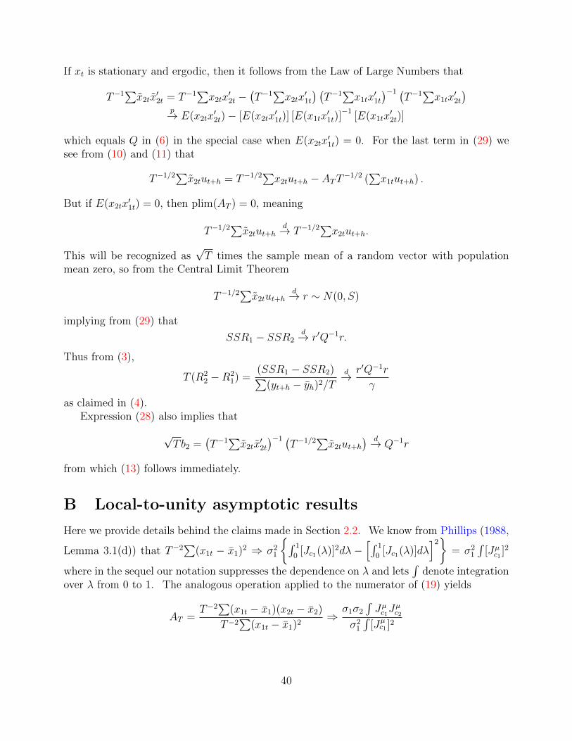
If xt is stationary and ergodic, then it follows from the Law of Large Numbers that

T−1∑x2tx

′2t = T−1

∑x2tx

′2t −

(T−1

∑x2tx

′1t

) (T−1

∑x1tx

′1t

)−1 (T−1

∑x1tx

′2t

)p→ E(x2tx

′2t)− [E(x2tx

′1t)] [E(x1tx

′1t)]−1

[E(x1tx′2t)]

which equals Q in (6) in the special case when E(x2tx′1t) = 0. For the last term in (29) we

see from (10) and (11) that

T−1/2∑x2tut+h = T−1/2

∑x2tut+h − ATT−1/2 (

∑x1tut+h) .

But if E(x2tx′1t) = 0, then plim(AT ) = 0, meaning

T−1/2∑x2tut+h

d→ T−1/2∑x2tut+h.

This will be recognized as√T times the sample mean of a random vector with population

mean zero, so from the Central Limit Theorem

T−1/2∑x2tut+h

d→ r ∼ N(0, S)

implying from (29) that

SSR1 − SSR2d→ r′Q−1r.

Thus from (3),

T (R22 −R2

1) =(SSR1 − SSR2)∑

(yt+h − yh)2/Td→ r′Q−1r

γ

as claimed in (4).Expression (28) also implies that

√Tb2 =

(T−1

∑x2tx

′2t

)−1 (T−1/2

∑x2tut+h

) d→ Q−1r

from which (13) follows immediately.

B Local-to-unity asymptotic results

Here we provide details behind the claims made in Section 2.2. We know from Phillips (1988,

Lemma 3.1(d)) that T−2∑

(x1t − x1)2 ⇒ σ21

{∫ 1

0[Jc1(λ)]2dλ−

[∫ 1

0[Jc1(λ)]dλ

]2}= σ2

1

∫[Jµc1 ]

2

where in the sequel our notation suppresses the dependence on λ and lets∫

denote integrationover λ from 0 to 1. The analogous operation applied to the numerator of (19) yields

AT =T−2

∑(x1t − x1)(x2t − x2)

T−2∑

(x1t − x1)2⇒

σ1σ2∫Jµc1J

µc2

σ21

∫[Jµc1 ]2

40

as claimed in (19). We also have from equation (2.17) in Stock (1994) that

T−1/2x2,[Tλ] ⇒ σ2Jc2(λ)

where [Tλ] denotes the largest integer less than Tλ. From the Continuous Mapping Theorem,

T−1/2x2 = T−3/2∑x2t =

∫ 1

0

T−1/2x2,[Tλ]dλ⇒ σ2

∫ 1

0

Jc2(λ)dλ.

Since x2t = x2t − x2 − AT (x1t − x1),

T−1/2x2,[Tλ] ⇒ σ2

{Jc2(λ)−

∫ 1

0

Jc2(s)ds− A[Jc1(λ)−

∫ 1

0

Jc1(s)ds

]}= σ2

{Jµc2(λ)− AJµc1(λ)

}= σ2Kc1,c2(λ)

T−2∑x22t =

∫ 1

0

{T−1/2x2,[Tλ]}2dλ⇒ σ22

∫ 1

0

{Kc1,c2(λ)}2 dλ. (30)

Note we can write ε1tε2tut

=

σ1 0 00 σ2 0

δσu 0√

1− δ2σu

v1tv2tv0t

where (v1t, v2t, v0t)

′ is a martingale-difference sequence with unit variance matrix. FromLemma 3.1(e) in Phillips (1988) we see

T−1∑x2tut+1 = T−1

∑[x2t − x2 − AT (x1t − x1)](δσuv1,t+1 +

√1− δ2σuv0,t+1)

⇒ δσ2σu

∫Kc1,c2dW1 +

√1− δ2σ2σu

∫Kc1,c2dW0. (31)

Recalling (28), under the null hypothesis the t-test of β2 = 0 can be written as

τ =

∑x2tut+1

{s2∑x22t}

1/2=

T−1∑x2tut+1

{s2T−2∑x22t}

1/2(32)

wheres2

p→ σ2u. (33)

Substituting (33), (31), and (30) into (32) produces

τ ⇒σ2σu

{δ∫Kc1,c2dW1 +

√1− δ2

∫Kc1,c2dW0

}{σ2uσ

22

∫(Kc1,c2)

2}1/2

as claimed in (20).Last we demonstrate that the variance of the variable Z1 defined in (21) exceeds unity. We

41

can write

Z1 =

∫ 1

0Jµc2(λ)dW1(λ){∫ 1

0[Kc1,c2(λ)]2dλ

}1/2−

A∫ 1

0Jµc1(λ)dW1(λ){∫ 1

0[Kc1,c2(λ)]2dλ

}1/2(34)

Consider the denominator in these expressions, and note that∫ 1

0

[Jµc2(λ)]2dλ =

∫ 1

0

[Jµc2(λ)− AJµc1(λ) + AJµc1(λ)]2dλ

=

∫ 1

0

[Kc1,c2(λ)]2dλ+

∫ 1

0

[AJµc1(λ)]2dλ

>

∫ 1

0

[Kc1,c2(λ)]2dλ

where the cross-product term dropped out in the second equation by the definition of A in(19). This means that the following inequality holds for all realizations:∣∣∣∣∣∣∣

∫ 1

0Jµc2(λ)dW1(λ){∫ 1

0[Kc1,c2(λ)]2dλ

}1/2

∣∣∣∣∣∣∣ >∣∣∣∣∣∣∣∫ 1

0Jµc2(λ)dW1(λ){∫ 1

0[Jµc2(λ)]2dλ

}1/2

∣∣∣∣∣∣∣ . (35)

Adapting the argument made in footnote 4, the magnitude inside the absolute-value operatoron the right side of (35) can be seen to have a N(0, 1) distribution. Inequality (35) thusestablishes that the first term in (34) has a variance that is greater than unity. The secondterm in (34) turns out to be uncorrelated with the first, and hence contributes additionalvariance to Z1, although we have found that the first term appears to be the most importantfactor.42 In sum, these arguments show that Var(Z1) > 1.

42These claims are based on moments of the respective functionals as estimated from discrete approximationsto the Ornstein-Uhlenbeck processes.

42

Table 1: Simulation study: size distortions of conventional t-test

δ = 0 δ = 0.8 δ = 1T ρ = 0.9 0.99 1 0.9 0.99 1 0.9 0.99 150 simulated 5.1 4.9 5.1 8.1 11.1 11.4 10.2 15.1 15.950 asymptotic 4.5 4.4 4.6 8.4 11.0 11.5 10.5 14.9 15.4

100 simulated 4.8 5.1 5.2 7.1 11.4 12.2 8.4 15.2 16.2100 asymptotic 4.5 4.7 4.8 7.0 11.1 11.9 8.4 15.0 16.0200 simulated 5.0 5.1 5.0 6.1 11.1 12.4 6.8 14.5 16.5200 asymptotic 4.9 4.9 4.9 6.2 10.7 12.0 7.2 14.6 16.6500 simulated 5.0 5.0 5.0 5.4 8.9 12.2 5.7 11.6 17.0500 asymptotic 5.0 4.8 4.9 5.4 9.2 12.3 5.8 11.6 16.9

True size (in percentage points) of a conventional t-test of H0 : β2 = 0 with nominal size of 5%, insimulated small samples and according to local-to-unity asymptotic distribution. δ determines thedegree of endogeneity, i.e., the correlation of x1t with the lagged error term ut. The persistence ofthe predictors is ρ1 = ρ2 = ρ. For details on the simulation study refer to main text.

Table 2: Simulation study: coefficient bias and standard error bias

δ = 1, γ = 0 δ = 0.8, γ = 0 δ = 0.8, γ = 0.8β1 β2 β1 β2 β1 β2

True coefficient 0.990 0.000 0.990 0.000 0.990 0.000Mean estimate 0.921 -0.000 0.936 -0.000 0.935 0.000Coefficient bias -0.069 -0.000 -0.054 -0.000 -0.055 0.000True standard error 0.053 0.055 0.049 0.049 0.082 0.083Mean OLS reported std. error 0.038 0.038 0.038 0.038 0.064 0.064Standard error bias -0.015 -0.017 -0.011 -0.011 -0.018 -0.019Size of t-test 0.344 0.155 0.223 0.111 0.155 0.112Size of bootstrap test 0.080 0.072 0.067Size of IM test 0.047 0.047 0.045

Analysis of bias in estimated coefficients and standard errors for regressions in small samples withT = 100 and ρ1 = ρ2 = 0.99, as well as estimated size of conventional t-test, bootstrap, and IMtests. For details on the simulation study refer to main text.

43

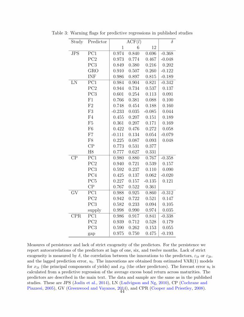
Table 3: Warning flags for predictive regressions in published studies

Study Predictor ACF(l) δ1 6 12

JPS PC1 0.974 0.840 0.696 -0.368PC2 0.973 0.774 0.467 -0.048PC3 0.849 0.380 0.216 0.202GRO 0.910 0.507 0.260 -0.122INF 0.986 0.897 0.815 -0.189

LN PC1 0.984 0.904 0.821 -0.342PC2 0.944 0.734 0.537 0.137PC3 0.601 0.254 0.113 0.091F1 0.766 0.381 0.088 0.100F2 0.748 0.454 0.188 0.160F3 -0.233 0.035 -0.085 0.044F4 0.455 0.207 0.151 0.189F5 0.361 0.207 0.171 0.169F6 0.422 0.476 0.272 0.058F7 -0.111 0.134 0.054 -0.079F8 0.225 0.087 0.093 0.048CP 0.773 0.531 0.377H8 0.777 0.627 0.331

CP PC1 0.980 0.880 0.767 -0.358PC2 0.940 0.721 0.539 0.157PC3 0.592 0.237 0.110 0.090PC4 0.425 0.137 0.062 -0.020PC5 0.227 0.157 -0.135 0.121CP 0.767 0.522 0.361

GV PC1 0.988 0.925 0.860 -0.312PC2 0.942 0.722 0.521 0.147PC3 0.582 0.233 0.094 0.105supply 0.998 0.990 0.974 0.035

CPR PC1 0.986 0.917 0.841 -0.338PC2 0.939 0.712 0.528 0.179PC3 0.590 0.262 0.153 0.055gap 0.975 0.750 0.475 -0.193

Measures of persistence and lack of strict exogeneity of the predictors. For the persistence wereport autocorrelations of the predictors at lags of one, six, and twelve months. Lack of strictexogeneity is measured by δ, the correlation between the innovations to the predictors, ε1t or ε2t,and the lagged prediction error, ut. The innovations are obtained from estimated VAR(1) modelsfor x1t (the principal components of yields) and x2t (the other predictors). The forecast error ut iscalculated from a predictive regression of the average excess bond return across maturities. Thepredictors are described in the main text. The data and sample are the same as in the publishedstudies. These are JPS (Joslin et al., 2014), LN (Ludvigson and Ng, 2010), CP (Cochrane andPiazzesi, 2005), GV (Greenwood and Vayanos, 2014), and CPR (Cooper and Priestley, 2008).

44

Table 4: Joslin-Priebsch-Singleton: predicting excess bond returns

Original sample: 1985–2008 Later sample: 1985–2013R2

1 R22 R2

2 − R21 R2

1 R22 R2

2 − R21

Two-year bondData 0.14 0.49 0.35 0.12 0.28 0.16Simple bootstrap 0.30 0.36 0.06 0.26 0.32 0.06

(0.06, 0.58) (0.11, 0.63) (-0.00, 0.22) (0.05, 0.51) (0.09, 0.56) (-0.00, 0.21)BC bootstrap 0.38 0.44 0.06 0.32 0.38 0.06

(0.07, 0.72) (0.13, 0.75) (-0.00, 0.23) (0.07, 0.60) (0.12, 0.64) (-0.00, 0.21)Ten-year bondData 0.20 0.37 0.17 0.20 0.28 0.08Simple bootstrap 0.26 0.32 0.07 0.24 0.30 0.06

(0.07, 0.48) (0.12, 0.54) (-0.00, 0.23) (0.06, 0.46) (0.11, 0.51) (-0.00, 0.21)BC bootstrap 0.27 0.34 0.08 0.26 0.33 0.07

(0.06, 0.50) (0.12, 0.57) (-0.00, 0.27) (0.06, 0.49) (0.11, 0.55) (-0.00, 0.23)Average two- through ten-year bondsData 0.19 0.39 0.20 0.17 0.25 0.08Simple bootstrap 0.28 0.35 0.07 0.24 0.30 0.06

(0.08, 0.50) (0.12, 0.56) (-0.00, 0.23) (0.05, 0.46) (0.10, 0.52) (-0.00, 0.21)BC bootstrap 0.30 0.37 0.07 0.27 0.33 0.07

(0.06, 0.55) (0.13, 0.61) (-0.00, 0.26) (0.05, 0.50) (0.12, 0.56) (-0.00, 0.24)

Adjusted R2 for regressions of annual excess bond returns on three PCs of the yield curve (R21) and

on three yield PCs together with the macro variables GRO and INF (R22), as well as the difference

in adjusted R2. GRO is the three-month moving average of the Chicago Fed National Activity

Index, and INF is one-year expected inflation measured by Blue Chip inflation forecasts. The data

used for the left half of the table is the original data set of Joslin et al. (2014); the data used in the

right half is extended to December 2013. The last panel shows results for the average excess bond

return for all bond maturities from two to ten years. The first row of each panel reports the values

of the statistics in the original data. The next three rows report bootstrap small-sample mean, and

the 95%-confidence intervals (in parentheses). The bootstrap simulations are obtained under the

null hypothesis that the macro variables have no predictive power. The bootstrap procedure for the

simple bootstrap and the bias-corrected (BC) bootstrap is described in the main text.

45

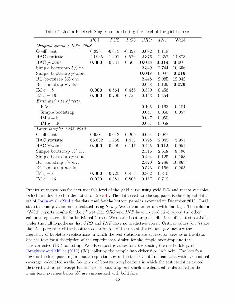
Table 5: Joslin-Priebsch-Singleton: predicting the level of the yield curve

PC1 PC2 PC3 GRO INF WaldOriginal sample: 1985–2008Coefficient 0.928 -0.013 -0.097 0.092 0.118HAC statistic 40.965 1.201 0.576 2.376 2.357 14.873HAC p-value 0.000 0.231 0.565 0.018 0.019 0.001Simple bootstrap 5% c.v. 2.349 2.744 10.306Simple bootstrap p-value 0.048 0.097 0.016BC bootstrap 5% c.v. 2.448 2.985 12.042BC bootstrap p-value 0.058 0.129 0.026IM q = 8 0.000 0.864 0.436 0.339 0.456IM q = 16 0.000 0.709 0.752 0.153 0.554Estimated size of tests

HAC 0.105 0.163 0.184Simple bootstrap 0.047 0.066 0.057IM q = 8 0.047 0.050IM q = 16 0.057 0.058

Later sample: 1985–2013Coefficient 0.958 -0.013 -0.209 0.024 0.087HAC statistic 65.682 1.258 1.453 0.798 2.045 5.951HAC p-value 0.000 0.209 0.147 0.425 0.042 0.051Simple bootstrap 5% c.v. 2.316 2.618 9.796Simple bootstrap p-value 0.494 0.125 0.158BC bootstrap 5% c.v. 2.470 2.789 10.867BC bootstrap p-value 0.523 0.156 0.203IM q = 8 0.000 0.725 0.815 0.302 0.310IM q = 16 0.020 0.381 0.805 0.157 0.719

Predictive regressions for next month’s level of the yield curve using yield PCs and macro variables

(which are described in the notes to Table 4). The data used for the top panel is the original data

set of Joslin et al. (2014); the data used for the bottom panel is extended to December 2013. HAC

statistics and p-values are calculated using Newey-West standard errors with four lags. The column

“Wald” reports results for the χ2 test that GRO and INF have no predictive power; the other

columns report results for individual t-tests. We obtain bootstrap distributions of the test statistics

under the null hypothesis that GRO and INF have no predictive power. Critical values (c.v.’s) are

the 95th percentile of the bootstrap distribution of the test statistics, and p-values are the

frequency of bootstrap replications in which the test statistics are at least as large as in the data.

See the text for a description of the experimental design for the simple bootstrap and the

bias-corrected (BC) bootstrap. We also report p-values for t-tests using the methodology of

Ibragimov and Muller (2010) (IM), splitting the sample into either 8 or 16 blocks. The last four

rows in the first panel report bootstrap estimates of the true size of different tests with 5% nominal

coverage, calculated as the frequency of bootstrap replications in which the test statistics exceed

their critical values, except for the size of bootstrap test which is calculated as described in the

main text. p-values below 5% are emphasized with bold face.

46

Tab

le6:

Ludvig

son-N

g:pre

dic

ting

exce

ssre

turn

susi

ng

PC

san

dm

acro

fact

ors

PC

1PC

2PC

3F

1F

2F

3F

4F

5F

6F

7F

8W

ald

A.

Ori

gin

al

sam

ple

:1964–2007

Coeffi

cien

t0.

136

2.0

52-5

.014

0.74

20.

146

-0.0

72-0

.528

-0.3

21-0

.576

-0.4

010.

551

HA

Cst

ati

stic

1.55

22.

595

2.72

41.

855

0.37

90.

608

1.91

21.

307

2.22

02.

361

3.03

642

.084

HA

Cp-v

alu

e0.

121

0.010

0.007

0.06

40.

705

0.54

30.

056

0.19

20.027

0.019

0.003

0.000

Boot

stra

p5%

c.v.

2.57

22.

580

2.24

12.

513

2.49

72.

622

2.44

62.

242

29.6

86B

oot

stra

pp-v

alu

e0.

140

0.76

10.

594

0.12

80.

301

0.09

20.

057

0.010

0.009

IMq

=8

0.001

0.001

0.22

50.

098

0.55

80.

579

0.08

80.

703

0.49

60.

085

0.32

4IM

q=

16

0.000

0.0

520.

813

0.22

80.

317

0.77

10.

327

0.35

80.

209

0.027

0.50

2E

stim

ate

dsi

zeof

test

sH

AC

0.13

10.

132

0.09

70.

124

0.12

60.

134

0.11

30.

086

0.33

5B

oot

stra

p0.

058

0.05

50.

053

0.06

10.

055

0.05

30.

049

0.04

60.

061

IMq

=8

0.05

10.

050

0.05

10.

049

0.04

90.

052

0.05

00.

042

IMq

=16

0.05

10.

048

0.05

10.

050

0.05

10.

045

0.05

50.

046

B.

Late

rsa

mple

:1985–2013

Coeffi

cien

t0.

157

1.1

822.

725

0.65

1-0

.274

0.14

7-0

.488

0.02

20.

334

0.03

5-0

.075

HA

Cst

ati

stic

1.50

61.

111

0.68

21.

652

0.26

70.

690

1.16

20.

038

1.86

60.

153

0.42

313

.766

HA

Cp-v

alu

e0.

133

0.26

80.

496

0.09

90.

789

0.49

10.

246

0.96

90.

063

0.87

80.

673

0.08

8B

oot

stra

p5%

c.v.

2.81

72.

908

2.51

62.

667

2.79

82.

468

2.36

52.

298

37.2

67B

oot

stra

pp-v

alu

e0.

224

0.84

40.

587

0.37

00.

973

0.13

60.

892

0.71

80.

495

IMq

=8

0.014

0.005

0.06

80.

139

0.51

10.

537

0.89

90.

767

0.14

40.

923

0.39

8IM

q=

16

0.024

0.1

850.

788

0.83

10.

636

0.92

30.

187

0.57

00.

882

0.70

30.

239

Pre

dic

tive

regr

essi

ons

for

annu

alex

cess

bon

dre

turn

s,av

erag

edov

ertw

o-th

rou

ghfi

ve-y

ear

bon

dm

atu

riti

es,

usi

ng

yie

ldP

Cs

and

fact

ors

from

ala

rge

dat

ase

tof

macr

ova

riab

les,

asin

Lu

dvig

son

and

Ng

(201

0).

Th

eto

pp

anel

show

sth

ere

sult

sfo

rth

eor

igin

ald

ata

set

use

dby

Lud

vig

son

an

dN

g(2

010)

;th

eb

otto

mp

anel

use

sa

dat

asa

mp

leth

atst

arts

in19

85an

den

ds

in20

13.

Th

eb

oot

stra

pis

asi

mple

boots

trap

wit

hou

tb

ias

corr

ecti

on.

For

ad

escr

ipti

onof

the

stat

isti

csin

each

row

,se

eth

en

otes

toT

able

5.p-v

alu

esb

elow

5%are

emp

hasi

zed

wit

hb

old

face

.

47

Table 7: Ludvigson-Ng: R2 for predicting excess returns using PCs and macro factors

R21 R2

2 R22 − R2

1

Original sample: 1964–2007Data 0.25 0.35 0.10Bootstrap 0.20 0.24 0.03

(0.05, 0.39) (0.08, 0.42) (-0.00, 0.11)Later sample: 1985–2013Data 0.14 0.18 0.04Bootstrap 0.26 0.29 0.03

(0.05, 0.49) (0.08, 0.51) (-0.01, 0.14)

Adjusted R2 for regressions of annual excess bond returns, averaged over two- through five-year

bonds, on three PCs of the yield curve (R21) and on three yield PCs together with eight macro

factors (R22), as well as the difference in R2. The top panel shows the results for the original data

set used by Ludvigson and Ng (2010); the bottom panel uses a data sample that starts in 1985 and

ends in 2013. For each data sample we report the values of the statistics in the data, and the mean

and 95%-confidence intervals (in parentheses) of the bootstrap small-sample distributions of these

statistics. The bootstrap simulations are obtained under the null hypothesis that the macro

variables have no predictive power. The bootstrap procedure, which does not include bias

correction, is described in the main text.

48

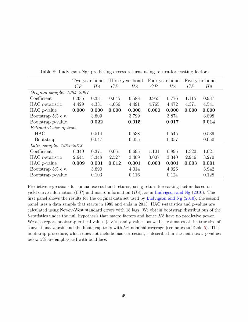
Table 8: Ludvigson-Ng: predicting excess returns using return-forecasting factors

Two-year bond Three-year bond Four-year bond Five-year bondCP H8 CP H8 CP H8 CP H8

Original sample: 1964–2007Coefficient 0.335 0.331 0.645 0.588 0.955 0.776 1.115 0.937HAC t-statistic 4.429 4.331 4.666 4.491 4.765 4.472 4.371 4.541HAC p-value 0.000 0.000 0.000 0.000 0.000 0.000 0.000 0.000Bootstrap 5% c.v. 3.809 3.799 3.874 3.898Bootstrap p-value 0.022 0.015 0.017 0.014Estimated size of tests

HAC 0.514 0.538 0.545 0.539Bootstrap 0.047 0.055 0.057 0.050

Later sample: 1985–2013Coefficient 0.349 0.371 0.661 0.695 1.101 0.895 1.320 1.021HAC t-statistic 2.644 3.348 2.527 3.409 3.007 3.340 2.946 3.270HAC p-value 0.009 0.001 0.012 0.001 0.003 0.001 0.003 0.001Bootstrap 5% c.v. 3.890 4.014 4.026 3.942Bootstrap p-value 0.103 0.116 0.124 0.128

Predictive regressions for annual excess bond returns, using return-forecasting factors based on

yield-curve information (CP ) and macro information (H8), as in Ludvigson and Ng (2010). The

first panel shows the results for the original data set used by Ludvigson and Ng (2010); the second

panel uses a data sample that starts in 1985 and ends in 2013. HAC t-statistics and p-values are

calculated using Newey-West standard errors with 18 lags. We obtain bootstrap distributions of the

t-statistics under the null hypothesis that macro factors and hence H8 have no predictive power.

We also report bootstrap critical values (c.v.’s) and p-values, as well as estimates of the true size of

conventional t-tests and the bootstrap tests with 5% nominal coverage (see notes to Table 5). The

bootstrap procedure, which does not include bias correction, is described in the main text. p-values

below 5% are emphasized with bold face.

49

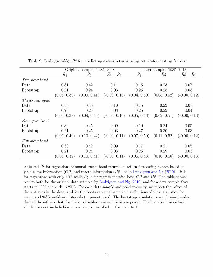
Table 9: Ludvigson-Ng: R2 for predicting excess returns using return-forecasting factors

Original sample: 1985–2008 Later sample: 1985–2013R2

1 R22 R2

2 − R21 R2

1 R22 R2

2 − R21

Two-year bondData 0.31 0.42 0.11 0.15 0.23 0.07Bootstrap 0.21 0.24 0.03 0.25 0.28 0.03

(0.06, 0.39) (0.09, 0.41) (-0.00, 0.10) (0.04, 0.50) (0.08, 0.52) (-0.00, 0.12)Three-year bondData 0.33 0.43 0.10 0.15 0.22 0.07Bootstrap 0.20 0.23 0.03 0.25 0.29 0.04

(0.05, 0.38) (0.09, 0.40) (-0.00, 0.10) (0.05, 0.48) (0.09, 0.51) (-0.00, 0.13)Four-year bondData 0.36 0.45 0.09 0.19 0.24 0.05Bootstrap 0.21 0.25 0.03 0.27 0.30 0.03

(0.06, 0.40) (0.10, 0.42) (-0.00, 0.11) (0.07, 0.50) (0.11, 0.52) (-0.00, 0.12)Five-year bondData 0.33 0.42 0.09 0.17 0.21 0.05Bootstrap 0.21 0.24 0.03 0.25 0.29 0.03

(0.06, 0.39) (0.10, 0.41) (-0.00, 0.11) (0.06, 0.48) (0.10, 0.50) (-0.00, 0.13)

Adjusted R2 for regressions of annual excess bond returns on return-forecasting factors based on

yield-curve information (CP ) and macro information (H8), as in Ludvigson and Ng (2010). R21 is

for regressions with only CP , while R22 is for regressions with both CP and H8. The table shows

results both for the original data set used by Ludvigson and Ng (2010) and for a data sample that

starts in 1985 and ends in 2013. For each data sample and bond maturity, we report the values of

the statistics in the data, and for the bootstrap small-sample distributions of these statistics the

mean, and 95%-confidence intervals (in parentheses). The bootstrap simulations are obtained under

the null hypothesis that the macro variables have no predictive power. The bootstrap procedure,

which does not include bias correction, is described in the main text.

50

Table 10: Cochrane-Piazzesi: in-sample evidence

PC1 PC2 PC3 PC4 PC5 Wald R21 R2

2 R22 −R2

1

Original sample: 1964–2003Data 0.127 2.740 -6.307 -16.128 -2.038 0.26 0.35 0.09HAC statistic 1.724 5.205 2.950 5.626 0.748 31.919HAC p-value 0.085 0.000 0.003 0.000 0.455 0.000Bootstrap 5% c.v./mean R2 2.253 2.236 8.464 0.21 0.21 0.01Bootstrap p-value/95% CIs 0.000 0.507 0.000 (0.05, 0.40) (0.06, 0.41) (0.00, 0.03)IM q = 8 0.002 0.030 0.873 0.237 0.233IM q = 16 0.000 0.004 0.148 0.953 0.283Estimated size of tests

HAC 0.085 0.083 0.114Bootstrap 0.046 0.053 0.055IM q = 8 0.040 0.050IM q = 16 0.043 0.049

Later sample: 1985–2013Data 0.104 1.586 3.962 -9.196 -9.983 0.14 0.17 0.03HAC statistic 1.619 2.215 1.073 1.275 1.351 4.174HAC p-value 0.106 0.027 0.284 0.203 0.178 0.124Bootstrap 5% c.v./mean R2 2.463 2.433 9.878 0.26 0.28 0.02Bootstrap p-value/95% CIs 0.301 0.273 0.272 (0.06, 0.49) (0.08, 0.50) (0.00, 0.05)IM q = 8 0.011 0.079 0.044 0.803 0.435IM q = 16 0.001 0.031 0.215 0.190 0.949

Predicting annual excess bond returns, averaged over two- through five-year bonds, using principalcomponents (PCs) of yields. The null hypothesis is that the first three PCs contain all the relevantpredictive information. The data used in the top panel is the same as in Cochrane and Piazzesi(2005)—see in particular their table 4. HAC statistics and p-values are calculated usingNewey-West standard errors with 18 lags. We also report the unadjusted R2 for the regressionusing only three PCs (R2

1) and for the regression including all five PCs (R22), as well as the

difference in these two. Bootstrap distributions are obtained under the null hypothesis, using thebootstrap procedure described in the main text (without bias correction). For the R2-statistics, wereport means and 95%-confidence intervals (in parentheses). For the HAC test statistics, bootstrapcritical values (c.v.’s) are the 95th percentile of the bootstrap distribution of the test statistics, andp-values are the frequency of bootstrap replications in which the test statistics are at least as largeas the statistic in the data. We also report p-values for t-tests using the methodology of Ibragimovand Muller (2010) (IM), splitting the sample into either 8 or 16 blocks. The last four rows in thefirst panel report bootstrap estimates of the true size of different tests with 5% nominal coverage,calculated as the frequency of bootstrap replications in which the test statistics exceed their criticalvalues, except for the size of bootstrap test which is calculated as described in the main text.p-values below 5% are emphasized with bold face.

51

Table 11: Cochrane-Piazzesi: out-of-sample forecast accuracy

n R22 R2

1 RMSE2 RMSE1 DM p-value RMSEmean(1) (2) (3) (4) (5) (6) (7) (8)2 0.321 0.260 2.120 1.769 2.149 0.034 1.0673 0.341 0.242 4.102 3.232 2.167 0.032 1.9464 0.371 0.266 5.848 4.684 2.091 0.039 2.9895 0.346 0.270 7.374 6.075 2.121 0.036 3.987average 0.351 0.264 4.845 3.917 2.133 0.035 2.385

In-sample vs. out-of-sample predictive power for excess bond returns (averaged across maturities)of a restricted model with three PCs and an unrestricted model with five PCs. The in-sampleperiod is from 1964 to 2002 (the last observation used by Cochrane-Piazzesi), and the out-of-sampleperiod is from 2003 to 2013. The second and third column show in-sample R2. The fourth and fifthcolumn show root-mean-squared forecast errors (RMSEs) of the two models. The column labeled“DM” reports the z-statistic of the Diebold-Mariano test for equal forecast accuracy, and thefollowing column the corresponding p-value. The last column shows the RMSE when forecasts arethe in-sample mean excess return.

52

Table 12: Greenwood-Vayanos: predictive power of Treasury bond supply

One-year Term Bondyield spread PC1 PC2 PC3 supply

Dependent variable: return on long-term bondCoefficient 1.212 0.026HAC t-statistic 2.853 3.104HAC p-value 0.004 0.002IM q = 8 0.030 0.795IM q = 16 0.001 0.925Dependent variable: return on long-term bondCoefficient 1.800 2.872 0.014HAC t-statistic 5.208 4.596 1.898HAC p-value 0.000 0.000 0.058IM q = 8 0.006 0.013 0.972IM q = 16 0.000 0.000 0.557Dependent variable: excess return on long-term bondCoefficient 0.168 5.842 -6.089 0.013HAC t-statistic 1.457 4.853 1.303 1.862HAC p-value 0.146 0.000 0.193 0.063IM q = 8 0.000 0.003 0.045 0.968IM q = 16 0.000 0.000 0.023 0.854Dependent variable: avg. excess return for 2-5 year bondsCoefficient 0.085 1.669 -4.632 0.004HAC statistic 1.270 3.156 2.067 1.154HAC p-value 0.204 0.002 0.039 0.249Bootstrap 5% c.v. 3.105Bootstrap p-value 0.448IM q = 8 0.005 0.134 0.714 0.494IM q = 16 0.008 0.011 0.611 0.980

Predictive regressions for annual bond returns using Treasury bond supply, as in Greenwood andVayanos (2014) (GV). The coefficients on bond supply in the first two panels are identical to thosereported in row (1) and (6) of Table 5 in GV. HAC t-statistics and p-values are constructed usingNewey-West standard errors with 36 lags, as in GV. The last two rows in each panel report p-valuesfor t-tests using the methodology of Ibragimov and Muller (2010), splitting the sample into either 8or 16 blocks. The sample period is 1952 to 2008. p-values below 5% are emphasized with bold face.

53

Table 13: Cooper-Priestley: predictive power of the output gap

gap CP CP PC1 PC2 PC3Coefficient -0.126OLS t-statistic 3.224HAC t-statistic 1.077HAC p-value 0.282Coefficient -0.120 1.588OLS t-statistic 3.479 13.541HAC t-statistic 1.244 4.925HAC p-value 0.214 0.000Coefficient 0.113 1.612OLS t-statistic 2.940 13.831HAC t-statistic 1.099 5.059HAC p-value 0.272 0.000Coefficient 0.147 0.001 0.043 -0.067OLS t-statistic 3.524 4.359 11.506 3.690HAC t-statistic 1.306 1.354 4.362 2.507HAC p-value 0.192 0.176 0.000 0.012Bootstrap 5% c.v. 2.933Bootstrap p-value 0.356IM q = 8 0.612 0.002 0.011 0.234IM q = 16 0.243 0.000 0.001 0.064

Predictive regressions for the one-year excess return on a five-year bond using the output gap, as inCooper and Priestley (2008) (CPR). CP is the Cochrane-Piazzesi factor after orthogonalizing itwith respect to gap, whereas CP is the usual Cochrane-Piazzesi factor. For the predictiveregression, gap is lagged one month, as in CPR. HAC standard errors are based on the Newey-Westestimator with 22 lags. The bootstrap procedure, which does not include bias correction, isdescribed in the main text. The sample period is 1952 to 2003. p-values below 5% are emphasizedwith bold face.

54

Figure 1: Simulation study: size of t-test and sample size

0 200 400 600 800 1000

0.00

0.05

0.10

0.15

0.20

Sample size

Em

piric

al s

ize

of te

st

ρ = 1, small−sample simulationsρ = 0.99, small−sample simulationsρ = 1, asymptotic distributionρ = 0.99, asymptotic distribution

True size of conventional t-test of H0 : β2 = 0 with nominal size of 5%, in simulated small samplesand according to local-to-unity asymptotic distribution, for different sample sizes, with δ = 1.Regressors are either random walks (ρ = 1) or stationary but highly persistent AR(1) processes(ρ = 0.99). For details on the simulation study refer to main text.

55

Figure 2: Cochrane-Piazzesi: predictive power of PCs across subsamples

1970 1980 1990 2000

−1

01

23

Endpoint for subsample

Sta

ndar

dize

d co

effic

ient

●

●

●

● ●

●●

●

PC1: t−stat = 4.74, p−value = 0.002

●

●

●

●

●

●

●

●

PC2: t−stat = 2.72, p−value = 0.030

●

●

●

●

●

●

●

●

PC3: t−stat = 0.17, p−value = 0.873PC4: t−stat = 1.29, p−value = 0.237PC5: t−stat = 1.31, p−value = 0.233

●

●

●

Regressor

PC1PC2PC3PC4PC5

Standardized coefficients on principal components (PCs) across eight different subsamples, ending

at the indicated point in time. Standardized coefficients are calculated by dividing through the

sample standard deviation of the coefficient across the eight samples. Text labels indicate

t-statistics and p-values of the Ibragimov-Mueller test with q = 8. Note that the t-statistics are

equal to means of the standardized coefficients multiplied by√

8. The data and sample period is

the same as in Cochrane and Piazzesi (2005).

56

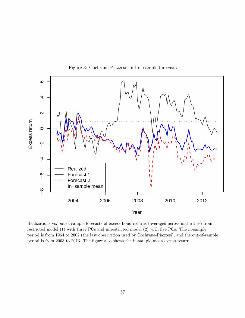
Figure 3: Cochrane-Piazzesi: out-of-sample forecasts

Year

Exc

ess

retu

rn

2004 2006 2008 2010 2012

−8

−6

−4

−2

02

46

RealizedForecast 1Forecast 2In−sample mean

Realizations vs. out-of-sample forecasts of excess bond returns (averaged across maturities) from

restricted model (1) with three PCs and unrestricted model (2) with five PCs. The in-sample

period is from 1964 to 2002 (the last observation used by Cochrane-Piazzesi), and the out-of-sample

period is from 2003 to 2013. The figure also shows the in-sample mean excess return.

57