Boosting with Structural Sparsity

John Duchi jduchi@cs.berkeley.edu

University of California, Berkeley

Berkeley, CA 94720 USA

Yoram Singer singer@google.com

Google

Mountain View, CA 94043 USA

Abstract

Despite popular belief, boosting algorithms and related coordinate descent methods are prone to

overfitting. We derive modifications to AdaBoost and related gradient-based coordinate descent

methods that incorporate, along their entire run, sparsity-promoting penalties for the norm of the

predictor that is being learned. The end result is a family of coordinate descent algorithms that

integrates forward feature induction and back-pruning through sparsity promoting regularization

along with an automatic stopping criterion for feature induction. We study penalties based on the

ℓ1, ℓ2, and ℓ∞ norm of the learned predictor and also introduce mixed-norm penalties that build

upon the initial norm-based penalties. The mixed-norm penalties facilitate structural sparsity

of the parameters of the predictor, which is a useful property in multiclass prediction and other

related learning tasks. We report empirical results that demonstrate the power of our approach in

building accurate and structurally sparse models from high dimensional data.

Keywords: Boosting, coordinate descent, group sparsity, feature induction and pruning.

1. Introduction and problem setting

Boosting is a highly effective and popular method for obtaining an accurate classifier from a set ofinaccurate predictors. Boosting algorithms construct high precision classifiers by taking a weightedcombination of base predictors, known as weak hypotheses. Rather than give a detailed overviewof boosting, we refer the reader to Meir and Ratsch (2003) or Schapire (2003) and the numerousreferences therein. While the analysis of boosting algorithms suggests that boosting attempts tofind large ℓ1 margin predictors subject to their weight vectors belonging to the simplex (Schapireet al., 1998), AdaBoost and boosting algorithms in general do not directly use the ℓ1-norm of theirweight vectors. Many boosting algorithms can also be viewed as forward-greedy feature inductionprocedures. In this view, the weak-learner provides new predictors which seem to perform welleither in terms of their error-rate with respect to the distribution that boosting maintains or interms of their potential of reducing the empirical loss (see, e.g. Schapire and Singer (1999)). Thus,once a feature is chosen, typically in a greedy manner, it is associated with a weight which remainsintact through the reminder of the boosting process. The original AdaBoost algorithm (Freundand Schapire, 1997) and its confidence-rated counterpart (Schapire and Singer, 1999) are notableexamples of this forward-greedy feature induction and weight assignment procedure, where thedifference between the two variants of AdaBoost boils down mostly to the weak-learner’s featurescoring and selection scheme.

The aesthetics and simplicity of AdaBoost and other forward greedy algorithms, such as Log-itBoost (Friedman et al., 2000), also facilitate a tacit defense from overfitting, especially whencombined with early stopping of the boosting process (Zhang and Yu, 2005). The empirical successof Boosting algorithms helped popularize the view that boosting algorithms are relatively resilientto overfitting. However, several researchers have noted the deficiency of the forward-greedy boosting

1

algorithm and suggested alternative coordinate descent algorithms, such as totally-corrective boost-ing (Warmuth et al., 2006) and a combination of forward induction with backward pruning (Zhang,2008). The algorithms that we present in this paper build on existing boosting and other coordinatedescent procedures while incorporating, throughout their run, regularization on the weights of theselected features. The added regularization terms influence both the induction and selection of newfeatures and the weight assignment steps. Moreover, as we discuss below, the regularization termmay eliminate (by assigning a weight of zero) previously selected features. The result is a simpleprocedure that includes forward induction, weight estimation, backward pruning, entertains conver-gence guarantees, and yields sparse models. Furthermore, the explicit incorporation of regularizationalso enables us to group features and impose structural sparsity on the learned weights, which is thefocus and one of the main contributions of the paper.

Our starting point is a simple yet effective modification to AdaBoost that incorporates, alongthe entire run, an ℓ1 penalty for the norm of the weight vector it constructs. The update we devisecan be used both for weight optimization and induction of new accurate hypotheses while taking theresulting ℓ1-norm into account, and it also gives a criterion for terminating the boosting process. Aclosely related approach was suggested by Dudık et al. (2007) in the context of maximum entropy.We provide new analysis for the classification case that is based on an abstract fixed-point theorem.This rather general theorem is also applicable to other norms, in particular the ℓ∞ norm whichserves as a building block for imposing structural sparsity.

We now describe more formally our problem setting. As mentioned above, our presentationand analysis is for classification settings, though our derivation can be easily extended to and usedin regression and other prediction problems (as demonstrated in the experimental section and theappendix). For simplicity of exposition, we assume that the class of weak hypotheses is finiteand contains n different hypotheses. We thus map each instance x to an n dimensional vector(h1(x), . . . , hn(x)), and we overload notation and simply denote the vector as x ∈ R

n. We discuss inSec. 8 the use of our framework in the presence of countably infinite features, also known as the task offeature induction. In the binary case, each instance xi is associated with a label yi ∈ −1,+1. Thegoal of learning is then to find a weight vector w such that the sign of w ·xi is equal to yi. Moreover,we would like to attain large inner-products so long as the predictions are correct. We build on thegeneralization of AdaBoost from Collins et al. (2002), which analyzes the the exponential-loss andthe log-loss, as the means to obtain this type of high confidence linear prediction. Formally, given asample S = (xi, yi)m

i=1, the algorithm focuses on finding w for which one of the following empiricallosses is small:

m∑

i=1

log (1 + exp(−yi(w · xi)) (LogLoss)m∑

i=1

exp (−yi(w · xi)) (ExpLoss) . (1)

We give our derivation and analysis for the log-loss as it also encapsulates the derivation for theexp-loss. We first derive an adaptation that incorporates the ℓ1-norm of the weight vector into theempirical loss,

Q(w) =

m∑

i=1

log (1 + exp(−yi(w · xi))) + λ‖w‖1. (2)

This problem is by no means new. It is often referred to as ℓ1-regularized logistic regression andseveral advanced optimization methods have been designed for the problem (see for instance Kohet al. (2007) and the references therein). This regularization has many advantages, including itsability to yield sparse weight vectors w and, under certain conditions, to recover the true sparsity ofw (Meinshausen and Buhlmann, 2006; Zhao and Yu, 2006). Our derivation shares similarity with theanalysis in Dudık et al. (2007) for maximum-entropy models, however, we focus on boosting and moregeneral regularization strategies. We provide an explicit derivation and proof for ℓ1 regularizationin order to make the presentation more accessible and to motivate the more complex derivationpresented in the sequel.

2

Next, we replace the ℓ1-norm penalty with an ℓ∞-norm penalty, proving an abstract primal-dualfixed point theorem on sums of convex losses with an ℓ∞ regularizer that we use throughout thepaper. While this penalty cannot serve as a regularization term in isolation, as it is oblivious to thevalue of most of the weights of the vector, it serves as an important building block for achievingstructural sparsity by using mixed-norm regularization, denoted ℓ1/ℓp. Mixed-norm regularizationis used when there is a partition of or structure over the weights that separates them into disjointgroups of parameters. Each group is tied together through an ℓp-norm regularizer. For concretenessand in order to leverage existing boosting algorithms, we specifically focus on settings in which wehave a matrix W = [w1 · · ·wk] ∈ R

n×k of weight vectors, and we regularize the weights in eachrow of W (denoted wj) together through an ℓp-norm. We derive updates for two important settingsthat generalize binary logistic-regression. The first is multitask learning (Obozinski et al., 2007). Inmultitask learning we have a set of tasks 1, . . . , k and a weight vector wr for each task. Withoutloss of generality, we assume that all the tasks share training examples (we could easily sum onlyover examples specific to a task and normalize appropriately). Our goal is to learn a matrix W thatminimizes

Q(W ) = L(W ) + λR(W ) =

m∑

i=1

k∑

r=1

log (1 + exp(−yi,r(wr · xi))) + λ

n∑

j=1

‖wj‖p . (3)

The other generalization we describe is the multiclass logistic loss. In this setting, we assumeagain there are k weight vectors w1, . . . ,wk that operate on each instance. Given an example xi,the classifier’s prediction is a vector [w1 · xi, . . . ,wk · xi], and the predicted class is the index ofthe inner-product attaining the largest of the k values, argmaxr wr · xi. In this case, the loss ofW = [w1 · · ·wk] is

Q(W ) = L(W ) + λR(W ) =m∑

i=1

log

1 +∑

r 6=yi

exp(wr · xi − wyi· xi)

+ λn∑

j=1

‖wj‖p . (4)

In addition to the incorporation of ℓ1/ℓ∞ regularization we also derive a completely new upperbound for the multiclass loss. Since previous multiclass constructions for boosting assume that theeach base hypothesis provides a different prediction per class, they are not directly applicable tothe more common multiclass setting discussed in this paper, which allocates a dedicated predictorper class. The end result is an efficient boosting-based update procedures for both multiclass andmultitask logistic regression with ℓ1/ℓ∞ regularization. Our derivation still follows the skeleton oftemplated boosting updates from Collins et al. (2002) in which multiple weights can be updated oneach round.

We then shift our focus to an alternative apparatus for coordinate descent with the log-loss thatdoes not stem from the AdaBoost algorithm. In this approach we bound above the log-loss by aquadratic function. We term the resulting update GradBoost as it updates one or more coordinatesin a fashion that follows gradient-based updates. Similar to the generalization of AdaBoost, westudy ℓ1 and ℓ∞ penalties by reusing the fixed-point theorem. We also derive an update withℓ2 regularization. Finally, we derive GradBoost updates with both ℓ1/ℓ∞ and ℓ1/ℓ2 mixed-normregularizations.

The end result of our derivations is a portfolio of coordinate descent-like algorithms for updatingone or more blocks of parameters (weights) for logistic-based problems. These types of problemsare often solved by techniques based on Newton’s method (Koh et al., 2007; Lee et al., 2006), whichcan become inefficient when the number of parameters n is large since they have complexity at leastquadratic (and usually cubic) in the number of features. In addition to new descent procedures, thebounds on the loss-decrease made by each update can serve as the means for selecting (inducing)new features. By re-updating previously selected weights we are able to prune-back existing fea-tures. Moreover, we can alternate between pure weight updates (restricting ourselves to the current

3

set of hypotheses) and pure induction of new hypotheses (keeping the weight of existing hypothesesintact). Further, our algorithms provide sound criteria for terminating boosting. As demonstratedempirically in our experiments, the end result of boosting with the structural sparsity based on ℓ1,ℓ1/ℓ2, or mixed-norm ℓ1/ℓ∞ regularizations is a compact and accurate model. The structural spar-sity is especially useful in complex prediction problems, such as multitask and multiclass learning,when features are expensive to compute. The mixed-norm regularization avoids the computation offeatures at test time since entire rows of W may set to be zero.

The paper is organized as follows. In the reminder of this section we give a brief overview of re-lated work. In Sec. 2 we describe the modification to AdaBoost which incorporates ℓ1 regularization.We then switch to ℓ∞ norm regularization in Sec. 3 and provide a general primal-dual theorem whichalso serves us in later sections. We use the two norms in Sec. 4, where describe our first structuralℓ1/ℓ∞ regularization. We next turn the focus to gradient-based coordinate descent and describe inSec. 5 the GradBoost update with ℓ1 regularization. In Sec. 6 we describe the GradBoost versionof the structural ℓ1/ℓ∞ regularization and in Sec. 7 a GradBoost update with ℓ1/ℓ2 regularization.In Sec. 8 we discuss the implications of the various updates for learning sparse models with forwardfeature induction and backward pruning, showing how to use the updates during boosting and fortermination of the boosting process. In Sec. 9 we briefly discuss the convergence properties of thevarious updates. Finally, in Sec. 10 we describe the results of experiments with binary classification,regression, multiclass, and multitask problems.

Related work: Our work intersects with several popular settings, builds upon existing work, andis related to numerous boosting and coordinate descent algorithms. It is clearly impossible to coverin depth the related work. We recap here the connections made thus far, and also give a shortoverview in attempt to distill the various contributions of this work. Coordinate descent algorithmsare well studied in the optimization literature. An effective use of coordinate descent algorithms formachine learning tasks was given for instance in Zhang and Oles (2001), which was later adaptedby Madigan and colleagues for text classification (2005). Our derivation follows the structure oftemplate-based algorithm from Collins et al. (2002) while incorporating regularization and scoringthe regularized base-hypotheses in a way analogous to the maximum-entropy framework of Dudıket al. (2007). The base GradBoost algorithm we derive shares similarity with LogitBoost (Friedmanet al., 2000), while similar bounding techniques to ours were first suggested by Dekel et al. (2005).

Learning sparse models for the logistic loss and other convex loss functions with ℓ1 regularizationis the focus of a voluminous amount of work in different research areas, from statistics to informationtheory. For instance, see Duchi et al. (2008) or Zhang (2008) and the numerous references thereinfor two recent machine learning papers that focus on ℓ1 domain constraints and forward-backwardgreedy algorithms in order to obtain sparse models with small ℓ1 norm. The alternating inductionwith weight-updates of Zhang (2008) is also advocated in the boosting literature by Warmuth andcolleagues, who term the approach “totally corrective” (2006). In our setting, the backward-pruningis not performed in a designated step or in a greedy manner but is rather a different facet of the weightupdate. Multiple authors have also studied the setting of mixed-norm regularization. Negahbanand Wainwright (2008) recently analyzed the structural sparsity characteristic of the ℓ1/ℓ∞ mixed-norm, and ℓ1/ℓ2-regularization was analyzed by Obozinski et al. (2008). Group Lasso and tiedmodels through absolute penalties are of great interest in the statistical estimation literature. Seefor instance Meinshausen and Buhlmann (2006); Zhao and Yu (2006); Zhao et al. (2006); Zhanget al. (2008), where the focus is on consistency and recovery of the true non-zero parameter ratheron efficient learning algorithms for large scale problems. The problem of simultaneously learningmultiple tasks is also the focus of many studies, see Evgeniou et al. (2005); Rakotomamonjy et al.(2008); Jacob et al. (2008) for recent examples and the references therein. In this paper we focus ona specific aspect of multiple task learning through structured regularization, which can potentiallybe used in other multitask problems such as multiple kernel learning.

4

Input: Training set S = (xi, yi)mi=1 ;

Update templates A ⊆ Rn+ s.t. ∀a ∈ A maxi

∑nj=1 aj |xi,j | ≤ 1

regularization λ ; number of rounds TFor t = 1 to T

// Compute importance weightsFor i = 1 to m

Set qt(i) = 11+exp(yi(wt·xi))

Choose a ∈ A// Compute feature correlationsFor j s.t. aj 6= 0

µ+j =

∑

i:yixi,j>0

qt(i)|xi,j | , µ−j =

∑

i:yixi,j<0

qt(i)|xi,j |

// Compute change in weights (δtj = 0 for all j s.t. aj = 0)

δtj =

−wtj if

∣∣∣µ+

j ewtj/aj − µ−

j e−wtj/aj

∣∣∣ ≤ λ

aj log−λ+

q

λ2+4µ+j

µ−

j

2µ−

j

if µ+j ewt

j/aj > µ−j e−wt

j/aj + λ

aj logλ+

q

λ2+4µ+j

µ−

j

2µ−

j

if µ+j ewt

j/aj < µ−j e−wt

j/aj − λ

wt+1 = wt + δt

Figure 1: AdaBoost for ℓ1-regularized log-loss.

2. AdaBoost with ℓ1 regularization

In this section we describe our ℓ1 infused modification to AdaBoost using the general frameworkdeveloped in Collins et al. (2002). In this framework, the weight update taken on each round ofboosting is based on a template that selects and amortizes the update over (possibly) multiplefeatures. The pseudocode for the algorithm is given in Fig. 1. On each round t of boosting animportance weight qt is calculated for each example. These weights are simply the probability thecurrent weight vector wt assigns to the incorrect label for example i, and they are identical to thedistribution defined over examples in the standard AdaBoost algorithm for the log-loss.

Let us defer the discussion on the use of templates to the end of Sec. 8 and assume that thetemplate a simply selects a single feature to examine, i.e. aj > 0 for some index j and ak = 0 forall k 6= j. Once a feature is selected we compute its correlation and inverse correlation with thelabel according to the distrubution qt, denoted by the variables µ+

j and µ−j . These correlations are

also calculated by AdaBoost. The major difference is the computation of the update to the weightj, denoted δt

j . The value of δtj of standard confidence-rated AdaBoost is 1

2 log(µ+j /µ−

j ), while ourupdate incorporates ℓ1-regularization with a multiplier λ. However, if we set λ = 0, we obtainthe weight update of AdaBoost. We describe a derivation of the updates of for AdaBoost withℓ1-regularization that constitutes the algorithm described in Fig. 1. While we present a completederivation in this section, the algorithm can be obtained as a special case of the analysis presentedin Sec. 3. The later analysis is rather lengthy and detailed, however, and we thus provide a concreteand simple analysis for the important case of ℓ1 regularization.

We begin by building on existing analyses of AdaBoost and show that each round of boosting isguaranteed to decrease the penalized loss. In the generalized version of boosting, originally describedby Collins et al. (2002), the booster selects a vector a from a set of templates A on each round ofboosting. The template selects the set of features, or base hypotheses, whose weight we update.Moreover, the template vector can may specify a different budget for each feature update so long asthe vector a satisfies the condition

∑

j aj |xi,j | ≤ 1. Classical boosting sets a single coordinate in the

5

vector a to a non-zero value, while the simultaneous update described in Collins et al. (2002) setsall coordinates of a to be the same. We start by recalling the progress bound for AdaBoost withthe log-loss when using a template vector.

Lemma 1 (Boosting progress bound (Collins et al., 2002)) Define importance weights qt(i) =1/(1 + exp(yiw

t · xi)) and correlations

µ+j =

∑

i:yixi,j>0

qt(i)|xi,j | and µ−j =

∑

i:yixi,j<0

qt(i)|xi,j | .

Let wt+1 = wt + δt such that δtj = ajd

tj and the vector a satisfies

∑

j aj |xi,j | ≤ 1. Then, the change

in the log-loss, ∆t = L(wt) − L(wt+1), between two iterations of boosting is lower bounded by

∆t ≥n∑

j=1

aj

(

µ+j

(

1 − e−dtj

)

+ µ−j

(

1 − edtj

))

=∑

j:aj>0

aj

(

µ+j

(

1 − e−δtj/aj

)

+ µ−j

(

1 − eδtj/aj

))

.

For convenience and completeness, we provide a derivation of the above lemma using the notationestablished in this paper in section A of the appendix. Since the ℓ1 penalty is an additive term, weincorporate the change in the 1-norm of w to bound the overall decrease in the loss when updatingwt to wt + δt with

Q(wt) − Q(wt+1) ≥n∑

j=1

aj

(

µ+j

(

1 − e−δtj/aj

)

+ µ−j

(

1 − eδtj/aj

))

− λ‖δt + wt‖1 + λ‖wt‖1 . (5)

By construction, Eq. (5) is additive in j, so long as aj > 0. We can thus maximize the progressindividually for each such index j,

ajµ+j

(

1 − e−δtj/aj

)

+ ajµ−j

(

1 − eδtj/aj

)

− λ∣∣δt

j + wtj

∣∣+ λ

∣∣wt

j

∣∣ . (6)

Omitting the index j and eliminating constants, we are left with the following minimization problemin δ:

minimizeδ

aµ+e−δ/a + aµ−eδ/a + λ |δ + w| . (7)

We now give two lemmas that aid us in finding the δ⋆ minimizing Eq. (7).

Lemma 2 If µ+ew/a − µ−e−w/a > 0, then the minimizing δ⋆ of Eq. (7) satisfies δ⋆ + w ≥ 0.Likewise, if µ+ew/a − µ−e−w/a < 0, then δ⋆ + w ≤ 0.

Proof Without loss of generality, we focus on the case when µ+ew/a > µ−e−w/a. Assume for thesake of contradiction that δ⋆ + w < 0. We now take the derivative of Eq. (7) with respect to δ,bearing in mind that the derivative of |δ + w| is −1. Equating the result to zero, we have

−µ+e−δ⋆/a + µ−eδ⋆/a − λ = 0 ⇒ µ+e−δ⋆/a ≤ µ−eδ⋆/a.

We assumed, however, that δ⋆ +w < 0, so that e(δ⋆+w)/a < 1 and e−(δ⋆+w)/a > 1. Thus, multiplyingthe left side of the above inequality by e(δ⋆+w)/a < 1 and the right by e−(δ⋆+w)/a > 1, we have that

µ+e−δ⋆/aeδ⋆/a+w/a < µ−eδ/ae−δ/a−w/a ⇒ µ+ew/a < µ−e−w/a.

This is a contradiction, so we must have that δ⋆ + w ≥ 0. The proof for the symmetric case followssimilarly.

In light of Lemma 2, we can eliminate the absolute value from the term |δ + w| in Eq. (7) andforce δ + w to take a certain sign. This property helps us in the proof of our second lemma.

6

Lemma 3 The optimal solution of equation Eq. (7) with respect to δ is δ⋆ = −w if and only if∣∣µ+ew/a − µ−e−w/a

∣∣ ≤ λ.

Proof Again, let δ⋆ denote the optimal solution of Eq. (7). Based on Lemma 2, we focus withoutloss of generality on the case where µ+ew/a > µ−e−w/a, which allows us to remove the absolutevalue from Eq. (7). We replace it with δ + w and add the constraint that δ + w ≥ 0, yielding thefollowing scalar optimization problem:

minimizeδ

aµ+e−δ/a + aµ−eδ/a + λ(δ + w) s.t. δ + w ≥ 0 .

The Lagrangian of the above problem is L(δ, β) = aµ+e−δ/a + aµ−eδ/a + λ(δ + w) − β(δ + w). Tofind the Lagrangian’s saddle point for δ we take its derivative and obtain ∂

∂δL(δ, β) = −µ+e−δ/a +

µ−eδ/a + λ− β. Let us first suppose that µ+ew/a − µ−e−w/a ≤ λ. If δ⋆ + w > 0 (so that δ⋆ > −w),then by the complementarity conditions for optimality (Boyd and Vandenberghe, 2004), β = 0,hence,

0 = −µ+e−δ⋆/a + µ−eδ⋆/a + λ > −µ+ew/a + µ−e−w/a + λ .

This implies that µ+ew/a − µ−e−w/a > λ, a contradiction. Thus, we must have that δ⋆ + w =0. To prove the other direction we assume the that δ⋆ = −w. Then, since β ≥ 0 we get−µ+ew/a + µ−e−w/a + λ ≥ 0, which implies that λ ≥ µ+ew/a − µ−e−w/a ≥ 0, as needed. Theproof for the symmetric case is analogous.

Equipped with the above lemmas, the update to wt+1j is straightforward to derive. Let us assume

without loss of generality that µ+j ewt

j/aj − µ−j e−wt

j/aj > λ, so that δ⋆j 6= −wj and δ⋆

j + wj > 0. Weneed to solve the following equation:

−µ+j e−δj/aj + µ−

j eδj/aj + λ = 0 or µ−j β2 + λβ − µ+

j = 0 ,

where β = eδj/aj . Since β is strictly positive, it is equal to the positive root of the above quadratic,yielding

β =−λ +

√

λ2 + 4µ+j µ−

j

2µ−j

⇒ δ⋆j = aj log

−λ +√

λ2 + 4µ+j µ−

j

2µ−j

. (8)

In the symmetric case, when δ⋆j + wt

j < 0, we get that δ⋆j = aj log

λ+q

λ2+4µ+j

µ−

j

2µ−

j

. Finally, when the

absolute value of the difference between µ+j exp(wt

j/aj) and µ−j exp(−wt

j/aj) is less than or equal

to λ, Lemma 3 implies that δ⋆j = −wt

j . When one of µ+j or µ−

j is zero but |µ+j ewt

j/aj | > λ of

|µ−j e−wt

j/aj | > λ, the solution is simpler. If µ−j = 0, then δ⋆

j = aj log(µ+j /λ), and when µ+

j = 0, then

δ⋆j = aj log(λ/µ−

j ). Omitting for clarity the cases when µ±j = 0, the different cases constitute the

core of the update given in Fig. 1.

3. Incorporating ℓ∞ regularization

Here we begin to lay the framework for multitask and multiclass boosting with mixed norm reg-ularizers. In particular, we derive boosting-style updates for the multitask and multiclass lossesof equations (3) and (4). The derivation in fact encompasses the derivation of the updates forℓ1-regularized AdaBoost, which we also discuss below.

Before we can derive updates for boosting, we make a digression to consider a more generalframework of minimizing a separable function with ℓ∞ regularization. In particular, the problem thatwe solve assumes that we have a sum of one-dimensional, convex, bounded below and differentiable

7

functions fj(d) (where we assume that if f ′j(d) = 0, then d is uniquely determined) plus an ℓ∞-

regularizer. That is, we want to solve

minimized

k∑

j=1

fj(dj) + λ ‖d‖∞ . (9)

The following theorem characterizes the solution d⋆ of Eq. (9), and it also allows us to developefficient algorithms for solving particular instances of Eq. (9). In the theorem, we allow the un-constrained minimizer of fj(dj) to be infinite, and we use the shorthand [k] to mean 1, 2, . . . , kand [z]+ = maxz, 0. The intuition behind the theorem and its proof is that we can move thevalues of d in their negative gradient directions together in a block, freezing entries of d that satisfyf ′

j(dj) = 0, until the objective in Eq. (9) begins to increase.

Theorem 4 Let dj satisfy f ′j(dj) = 0. The optimal solution d⋆ of Eq. (9) satisfies the following

properties:

(i) d⋆ = 0 if and only if∑k

j=1 |f ′j(0)| ≤ λ.

(ii) For all j, f ′j(0)d⋆

j ≤ 0 and f ′j(d

⋆j )d

⋆j ≤ 0.

(iii) Let B =j : |d⋆

j | = ‖d⋆‖∞

and U = [k] \ B. Then

(a) For all j ∈ U , dj = d⋆j and f ′

j(d⋆j ) = 0.

(b) For all j ∈ B, |dj | ≥ |d⋆j | = ‖d⋆‖∞

(c) When d⋆ 6= 0,∑k

j=1 |f ′j(d

⋆j )| =

∑

j∈B |f ′j(d

⋆j )| = λ.

Proof Before proving the particular statements (i), (ii), and (iii) above, we perform a few prelimi-nary calculations with the Lagrangian of Eq. (9) that will simplify the proofs of the various parts.Minimizing

∑

j fj(dj) + λ ‖d‖∞ is equivalent to solving the following problem:

minimize∑k

j=1 fj(dj) + λξ

s.t. −ξ ≤ dj ≤ ξ ∀j, and ξ ≥ 0 .(10)

Although the positivity constraint on ξ is redundant, it simplifies the proof. To solve Eq. (10), weintroduce Lagrange multiplier vectors α 0 and β 0 for the constraints that −ξ ≤ dj ≤ ξ andthe multiplier γ ≥ 0 for the non-negativity of ξ. This gives the Lagrangian

L(d, ξ,α,β, γ) =

k∑

j=1

fj(dj) + λξ +

k∑

j=1

αj(dj − ξ) +

k∑

j=1

βj(−dj − ξ) − γξ . (11)

To find the saddle point of Eq. (11), we take the infimum of L with respect to ξ, which is −∞ unless

λ −k∑

j=1

αj −k∑

j=1

βj − γ = 0 . (12)

The non-negativity of γ implies that∑k

j=1 αj + βj ≤ λ. Complimentary slackness (Boyd and

Vandenberghe, 2004) then shows that if ξ > 0 at optimum, γ = 0 so that∑k

j=1 βj + αj = λ.We are now ready to start proving assertion (i) of the theorem. By taking derivatives of L to

find the saddle point of the primal-dual problem, we know that at the optimal point d⋆ the followingequality holds:

f ′j(d

⋆j ) − βj + αj = 0 . (13)

8

Suppose that d⋆ = 0 so that the optimal ξ = 0. By Eq. (12), Eq. (13), and complimentary slacknesson α and β we have

k∑

j=1

|f ′j(0)| =

k∑

j=1

|αj − βj | ≤k∑

j=1

αj + βj ≤ λ .

This completes the proof of the first direction of (i). We now prove the converse. Suppose that∑k

j=1 |f ′j(0)| ≤ λ. In this case, if we set αj =

[−f ′

j(0)]

+and βj =

[f ′

j(0)]

+, we have |f ′

j(0)| = βj +αj

and∑k

j=1 αj + βj ≤ λ. Simply setting ξ = 0 and letting γ = λ −∑kj=1(αj + βj) ≥ 0, we have

∑kj=1 αj + βj + γ = λ. The KKT conditions for the problem are thus satisfied and 0 is the optimal

solution. This proves part (i) of the theorem.We next prove statement (ii) of the theorem. We begin by proving that if f ′

j(0) ≤ 0, then d⋆j ≥ 0

and similarly, that if f ′j(0) ≥ 0, d⋆

j ≤ 0. If f ′j(0) = 0, we could choose d⋆

j = 0 without incurringany penalty in the ℓ∞ norm. Thus, suppose that f ′

j(0) < 0. Then, we have fj(−δ) > fj(0) for allδ > 0, since the derivative of a convex function is non-decreasing. As such, the optimal setting ofdj must be non-negative. The argument for the symmetric case is similar, and we have shown thatf ′

j(0)d⋆j ≤ 0.

The second half of (ii) is derived similarly. We know from Eq. (13) that f ′j(d

⋆j ) = βj − αj . If

f ′j(0) < 0, the complimentary slackness condition implies that βj = 0 and αj ≥ 0. These two

properties together imply that f ′j(d

⋆j ) ≤ 0 whenever f ′

j(0) < 0. An analogous argument is truewhen f ′

j(0) > 0, which implies that f ′j(d

⋆j ) ≥ 0. Combining these properties with the statements of

previous paragraph, we have that f ′j(d

⋆j )d

⋆j ≤ 0. This completes the proof of part (ii) of the theorem.

Let us now consider part (iii) of the theorem. If d⋆ = 0, then the set U is empty, thus (a), (b),and (c) are trivially satisfied. For the remainder of the proof, we assume that d⋆ 6= 0. In this casewe must have ξ > 0, and complimentary slackness guarantees that γ = 0 and that at most one ofαj and βj are nonzero. Consider the indices in U , that is, j such that −ξ < d⋆

j < ξ. For any suchindex j, both αj and βj must be zero by complimentary slackness. Therefore, from Eq. (13) we

know f ′j(d

⋆j ) = 0. The assumption that dj is the unique minimizer of fj means that d⋆

j = dj , i.e.coordinates not at the bound ξ simply take their unconstrained solutions. This proves point (a) ofpart (iii).

We now consider point (b) of statement (iii) from the theorem. For j ∈ B, we have |dj | ≥ ξ.

Otherwise we could take d⋆j = dj and have |dj | < ξ. This clearly decreases the objective for fj

because fj(dj) < fj(d⋆j ). Further, |dj | < ξ so the constraints on ξ would remain intact, and we

would have j 6∈ B. We therefore must have |dj | ≥ ξ = |d⋆j |, which finishes the proof of part (b).

Finally, we arrive at part (c) of statement (iii). Applying Eq. (12) with γ = 0, we have λ =∑k

j=1 αj + βj , and applying Eq. (13) gives

k∑

j=1

|f ′j(d

⋆j )| =

k∑

j=1

|βj − αj | =

k∑

j=1

αj + βj = λ . (14)

This proves point (c) for the first of the two sums. Next, we divide the solutions d⋆j into the two

sets B (for bounded) and U (for unbounded), where

B = j : |d⋆j | = ξ = ‖d⋆‖∞ and U = j : |d⋆

j | < ξ.

Clearly, B is non-empty, since otherwise we could decrease ξ in the objective from Eq. (10). Recallingthat for j ∈ U , f ′

j(d⋆j ) = 0, Eq. (14) implies that the second equality of point (c) holds, namely

k∑

j=1

|f ′j(d

⋆j )| =

∑

j∈B

|f ′j(d

⋆j )| +

∑

j∈U

|f ′j(d

⋆j )|

︸ ︷︷ ︸

=0

= λ .

9

Input: Convex functions frkr=1, regularization λ

If∑k

r=1 |f ′r(0)| ≤ λ

Return d⋆ = 0// Find sign of optimal solutionsSet sr = − sign(f ′

r(0))// Get ordering of unregularized solutions

Solve dr = argmind fr(srd)

// We have d(1) ≥ d(2) ≥ . . . ≥ d(k)

Sort dr (descending) into d(r); d(k+1) = 0For l = 1 to k

Solve for ξ such that∑l

i=1 f ′(i)(siξ) = −λ

If ξ ≥ d(l+1)

Break

Return d⋆ such that d⋆r = sr mindr, ξ

Figure 2: Algorithm for minimizing∑

r fr(dr) + λ ‖d‖∞.

In Fig. 2, we present a general algorithm that builds directly on the implications of Thm. 4 forfinding the minimum of

∑

j fj(dj)+λ ‖d‖∞. The algorithm begins by flipping signs so that all dj ≥ 0(see part (ii) of the theorem). It then iteratively adds points to the bounded set B, starting from thepoint with largest unregularized solution d(1) (see part (iii) of the theorem). When the algorithmfinds a set B and bound ξ = ‖d‖∞ so that part (iii) of the theorem is satisfied (which is guaranteedby (iii.b), since all indices in the bounded set B must have unregularized solutions greater than thebound ‖d⋆‖∞), it terminates. Note that the algorithm naıvely has runtime complexity of O(k2). Inthe following sections, we show that this complexity can be brought down to O(k log k) by exploitingthe structure of the functions fj that we consider (this could be further decreased to O(k) usinggeneralized median searches, however, this detracts from the main focus of this paper).

Revisiting AdaBoost with ℓ1-regularization We can now straightforwardly derive lemmas 2and 3 as special cases of Theorem 4. Recall the ℓ1-regularized minimization problem we faced for theexponential loss in Eq. (7): we had to minimize a function of the form aµ+e−δ/a+aµ−eδ/a+λ|δ+w|.Replacing δ + w with θ, this minimization problem is equivalent to minimizing

aµ+ew/ae−θ/a + aµ−e−w/aeθ/a + λ|θ|.

The above problem amounts to a simple one-dimensional version of the type of problem consideredin Thm. 4. We take the derivative of the first two terms with respect to θ, which at θ = 0 is−µ+ew/a + µ−e−w/a. If this term is positive, then θ⋆ ≤ 0, otherwise, θ⋆ ≥ 0. This result isequivalent to the conditions for δ⋆ + w ≤ 0 and δ⋆ + w ≥ 0 in Lemma 2. Lemma 3 can also beobtained as an immediate corollary of Thm. 4 since θ⋆ = 0 if and only if |µ+ew/a − µ−e−w/a| ≤λ, which implies that w + δ⋆ = 0. The solution in Eq. (8) amounts to finding the θ such that|µ+ew/ae−θ/a − µ−e−w/aeθ/a| = λ.

4. AdaBoost with ℓ1/ℓ∞ mixed-norm regularization

In this section we build on the results presented in the previous sections and present extensions ofthe AdaBoost algorithm to multitask and multiclass problems with mixed-norm regularization givenin Eq. (3) and Eq. (4).

10

We start with a bound on the logistic loss to derive boosting-style updates for the mixed-normmultitask loss of Eq. (3) with p = ∞. To remind the reader, the loss we consider is

Q(W ) = L(W ) + λR(W ) =

m∑

i=1

k∑

r=1

log (1 + exp(−yi,r(wr · xi))) + λ

n∑

j=1

‖wj‖∞ .

In the above, wr represents the rth column of W while wj represents the jth row. In order to extendthe boosting algorithm from Fig. 1, we first need to extend the progress bounds for binary logisticregression to the multitask objective.

The multitask loss is decomposable into sums of losses, one per task. Hence, for each separatetask we obtain the same bound as that of Lemma 1. However, we now must update rows wj fromthe matrix W while taking into account the mixed-norm penalty. Given a row j, we calculateimportance weights qt(i, r) for each example i and task r as qt(i, r) = 1/(1 + exp(yi,rwr · xi)) andthe correlations µ±

r,j for each task r through a simple generalization of the correlations in Lemma 1as

µ+r,j =

∑

i:yi,rxi,j>0

qt(i, r)|xi,j | and µ−r,j =

∑

i:yi,rxi,j<0

qt(i, r)|xi,j | .

Defining δj = [δj,1 · · · δj,k] and applying lemma 1 yields that when we update W t+1 = W t +[δt

1 · · · δtn]⊤, we can lower bound the change in the loss ∆t = L(W t+1) − L(W t) between iterations

t and t + 1 by

∆t ≥n∑

j=1

aj

k∑

r=1

(

µ+r,j

(

1 − e−δtj,r/aj

)

+ µ−r,j

(

1 − eδtj,r/aj

))

. (15)

As before, the template vector should satisfy the constraint that∑

j aj |xi,j | ≤ 1 for all i.Before proceeding to the specifics of the algorithm, we revisit the multiclass objective from Eq. (4)

and bound it as well. Again, we have

Q(W ) = L(W ) + λR(W ) =

m∑

i=1

log

1 +∑

r 6=yi

exp(wr · xi − wyi· xi)

+ λ

n∑

j=1

‖wj‖∞ .

A change in the definition of the importance weights to be the probability that the weight matrixW assigns to a particular class, along with an updated definition of the correlations µ±

r,j , gives us abound on the change in the multiclass loss. In particular, the following lemma modifies and extendsthe multiclass boosting bounds of Collins et al. (2002).

Lemma 5 (Multiclass boosting progress bound) Let qt(i, r) denote importance weights for eachexample index i and class index r ∈ 1, . . . , k, where

qt(i, r) =exp(wt

r · xi)∑

l exp(wtl · xi)

.

Define the importance-weighted correlations as

µ+r,j =

∑

i:yi 6=r,xi,j<0

qt(i, r)|xi,j | +∑

i:yi=r,xi,j>0

(1 − qt(i, yi))|xi,j |

µ−r,j =

∑

i:yi 6=r,xi,j>0

qt(i, r)|xi,j | +∑

i:yi=r,xi,j<0

(1 − qt(i, yi))|xi,j | .

Let the update to the jth row of the matrix W t is wt+1j = wt

j + δtj and that the vector a satisfies

maxi 2∑

j aj |xi,j | ≤ 1. Then the change in the multiclass logistic loss, ∆t = L(W t+1) − L(W t), is

11

lower bounded by

∆t ≥n∑

j=1

aj

k∑

r=1

(

µ+r,j

(

1 − e−δtj,r/aj

)

+ µ−r,j

(

1 − eδtj,r/aj

))

. (16)

The proof of the lemma is provided in Appendix A. The standard boosting literature usually assumesthat instead of having multiple class vectors wr, there is a single vector w and that features havedifferent outputs per-class, denoted h(xi, r). Our setting instead allows single view of xi withmultiple prediction vectors wr, arguably a more natural (and common) parameterization. Withthe lemma in place, we note that the boosting bounds we have achieved for the multitask loss inEq. (15) and the multiclass loss in Eq. (16) are syntactically identical. They differ only in theircomputation of the importance weights and weighted correlations. These similarities allow us toattack the boosting update for both together, deriving one efficient algorithm for ℓ1/ℓ∞-regularizedboosting based on a corollary to Theorem 4 and the algorithm of Fig. 2.

Now we proceed with the derivation of AdaBoost with structural regularization. Adding ℓ∞-regularization terms to Eq. (15) and Eq. (16), we have

Q(W t) − Q(W t+1) ≥n∑

j=1

aj

k∑

r=1

(

µ+r,j

(

1 − e−δj,r/aj

)

+ µ−r,j

(

1 − eδj,r/aj

))

−λ

n∑

j=1

∥∥wt

j + δj

∥∥∞

+ λ

n∑

j=1

∥∥wt

j

∥∥∞

. (17)

For simplicity of our derivation, we focus on updating a single row j in W , and we temporarilyassume that wt

j = 0. We make the substitution ajdr = δj,r. Using these assumptions and a fewsimple algebraic manipulations, we find that we need to solve the following minimization problem:

minimized

k∑

r=1

µ+r e−dr + µ−

r edr + λ ‖d‖∞ . (18)

First, we note that the objective function of Eq. (18) is separable in d with an ℓ∞-regularizationterm. Second, the derivative of each of the terms, dropping the regularization term, is −µ+

r e−dr +µ−

r edr . Third, the un-regularized minimizers are dr = 12 log(µ+

r /µ−r ), where we allow dr = ±∞. We

immediately have the following corollary to Theorem 4:

Corollary 6 The optimal solution d⋆ of Eq. (18) is d⋆ = 0 if and only if∑k

r=1 |µ+r − µ−

r | ≤ λ.Assume without loss of generality that µ+

r ≥ µ−r . When d⋆ 6= 0, there are sets B = r : |d⋆

r | =‖d⋆‖∞ and U = [k] \ B such that

(a) For all r ∈ U , µ+r e−d⋆

r − µ−r ed⋆

r = 0

(b) For all r ∈ B, |dr| ≥ |d⋆r | = ‖d⋆‖∞

(c)∑

r∈B µ+r e−‖d⋆‖

∞ − µ−r e‖d⋆‖

∞ − λ = 0.

Based on the corollary above, we can derive an efficient procedure that first sorts the indices in[k] by the magnitude of the unregularized solution dr (we can assume that µ+

r ≥ µ−r and flip signs at

the end as in Fig. 2) to find d(ρ), where d(ρ) is the ρth largest unregularized solution. The algorithmthen solves the following equation in d for each ρ ∈ [k],

e−d∑

r:dr≥d(ρ)

µ+r − ed

∑

r:dr≥d(ρ)

µ−r − λ = 0 . (19)

12

This process continues until we find an index ρ such that the solution d⋆ for Eq. (19) satisfiesd⋆ ≥ d(ρ+1). To develop an efficient algorithm, we define

M±ρ =

∑

r:dr≥d(ρ)

µ±r .

In order to solve Eq. (19) for each d, we can apply the reasoning for Eq. (8) and find

d⋆ = log−λ +

√

λ2 + 4M+ρ M−

ρ

2M−ρ

. (20)

When M−ρ = 0, we get d⋆ = log(λ/M+

ρ ). We can use Eq. (20) successively in the algorithm of Fig. 2

by setting M±ρ+1 = M±

ρ + µ±(ρ). To recap, by sorting dr = 1

2 log(µ+r /µ−

r ) and incrementally updating

M±ρ , we can use the algorithm of Fig. 2 to solve the multiclass and multitask extensions of AdaBoost

with ℓ1/ℓ∞-regularization.It remains to show how to solve the more general update from Eq. (17). In particular, we would

like to find the minimum of

a

k∑

r=1

(µ+

r e−dr + µ−r edr

)+ λ ‖w + ad‖∞ . (21)

We can make the transformation γr = wr/a+dr, which reduces our problem to finding the minimizerof

k∑

r=1

(

µ+r ewr/ae−γr + µ−

r e−wr/aeγr

)

+ λ ‖γ‖∞

with respect to γ. This minimization problem can be solved by using the same sorting-basedapproach as in the prequel, and we then recover d⋆ = γ⋆ − w/a.

Combining our reasoning for the multiclass and multitask losses, we obtain an algorithm thatsolves both problems by appropriately setting µ±

r,j while using the algorithm of Fig. 2. The combinedalgorithm for both problems is presented in Fig. 3.

5. Gradient Boosting with ℓ1 regularization

We have presented thus far algorithms and analyses that are based on the original AdaBoost algo-rithm. In this section we shift our attention to a lesser known approach and derive additive updatesfor the logistic-loss based on quadratic upper bounds. The bounding techniques we use are basedon those described by Dekel et al. (2005). We follow popular naming conventions and term thesemethods GradBoost for their use of gradients and bounds on the Hessian. We would like to notethat the resulting algorithms do not necessarily entertain the weak-to-strong learnability propertiesof AdaBoost. Generally speaking, our methods can be view as guarded (block) coordinate descentmethods for binary and multivariate logistic losses. GradBoost gives a different style of updates,which in some cases may be faster than the AdaBoost updates, while still enjoying the same featureinduction benefits and convergence guarantees as the previous algorithms (see the later sections 8and 9). Furthermore, the use of the quadratic bounds on the logistic functions allows us to performboosting-style steps with ℓ2 and ℓ22 regularization in addition to the ℓ1 and ℓ∞ regularization studiedabove. Concretely, we use bounds of the form

L(w + δej) ≤ L(w) + ∇L(w) · ejδ +1

2δej · Dejδ,

where D is chosen to upper bound ∇2L(w). In the binary case, for example, D = diag(1/4∑m

i=1 x2i,j).

13

Input: Training set S = (xi,yi)mi=1

Regularization λ, number of rounds TUpdate templates A ⊆ R

n+ s.t.

∀a ∈ A maxi

∑nj=1 aj |xi,j | ≤ 1 [MT]

∀a ∈ A maxi

∑nj=1 aj |xi,j | ≤ 1/2 [MC]

For t = 1 to TChoose j ∈ 1, . . . , nFor i = 1 to m and r = 1 to k

Set qt(i, r) =

exp(wr·xi)

P

l exp(wl·xi)[MC]

11+exp(yi,r(wt

r·xi))[MT]

For r = 1 to k

µ+r,j =

∑

i:yi,rxi,j>0

qt(i, r)|xi,j | [MT]

∑

i:yi=r,xi,j>0

(1 − qt(i, yi))|xi,j | +∑

i:yi 6=r,xi,j<0

qt(i, r)|xi,j | [MC]

µ−r,j =

∑

i:yi,rxi,j<0

qt(i, r)|xi,j | [MT]

∑

i:yi=r,xi,j<0

(1 − qt(i, yi))|xi,j | +∑

i:yi 6=r,xi,j>0

qt(i, r)|xi,j | [MC]

Minimize for δj ∈ Rk such that aj 6= 0 (use Alg. 2)

∑nj=1 aj

∑kr=1

[µ+

r,je−δj,r/aj + µ−

r,jeδj,r/aj

]+ λ

∥∥wt

j + ajδj

∥∥∞

Update

W t+1 = W t + [δ1 · · · δn]⊤

Figure 3: Boosting algorithm for solving ℓ1/ℓ∞-regularized multitask or multiclass logistic regressionusing Alg. 2

We first focus on the binary logistic loss of Eq. (2). GradBoost, similar to AdaBoost, uses atemplate vector a to parameterize updates to the weight vectors. We can thus perform updatesranging from a single feature, analogous to the AdaBoost algorithm, to all the features, in a mannersimilar to the parallel version of AdaBoost from Collins et al. (2002). The following lemma providesa quantitative statement on the amount of progress that GradBoost can make. We provide a proofof the lemma in Appendix B.

Lemma 7 (GradBoost Progress Bound) Denote by g the gradient of the logistic loss so thatgj = −µ+

j + µ−j , where µ+

j , µ−j are defined as in lemma 1. Assume that we are provided an update

template a ∈ Rn+ such that

∑

i,j ajx2i,j ≤ 1. Let wt+1 = wt + δt and δt

j = ajdtj. Then the change,

∆t = L(wt)−L(wt+1), in the logistic-loss between two consecutive iterations of GradBoost is lowerbounded by

∆t ≥ −n∑

j=1

aj

(

gjdtj +

(dtj)

2

8

)

= −∑

j:aj>0

(

gjδtj +

(δtj)

2

8aj

)

.

The assumption on a at a first glance seems strong, but is in practice no stronger than the assumptionon the template vectors for AdaBoost in Lemma 1. AdaBoost requires that maxi

∑nj=1 aj |xi,j | ≤ 1,

while GradBoost requires a bound on the average for each template vector. Indeed, had we usedthe average logistic loss, dividing L(w) by m, and assumed that maxj |xi,j | = 1, AdaBoost andGradBoost would have shared the same set of possible update templates. Note that the minus sign

14

in front of the bound also seems a bit odd upon a first look. However, we choose δt in the oppositedirection of g to decrease the logistic-loss substantially, as we show in the sequel.

To derive a usable bound for GradBoost with ℓ1-regularization, we replace the progress bound inlemma 7 with a bound dependent on wt+1 and wt. Formally, we rewrite the bound by substitutingwt+1 − wt for δt. Recalling Eq. (2) to incorporate ℓ1-regularization, we get

Q(wt+1)−Q(wt) ≤∑

j:aj>0

gj(wt+1j −wt

j) +1

8

∑

j:aj>0

1

aj(wt+1

j −wtj)

2 + λ∥∥wt+1

∥∥

1− λ

∥∥wt

∥∥

1. (22)

As the bound in Eq. (22) is separable in each wj , we can decompose it and minimize with respectto the individual entries of w. Performing a few algebraic manipulations and letting w be short forwt+1

j , we want to minimize(

gj −wt

j

4aj

)

w +1

8ajw2 + λ|w| . (23)

The minimizer of Eq. (23) can be derived using Lagrange multipliers or subgradient calculus. Instead,we describe a solution that straightforwardly builds on Thm. 4.

First, note that when aj = 0, we simply set wt+1j = wt

j . We can thus focus on an index j suchthat aj > 0. Multiplying Eq. (23) by 4aj , the quadratic form we need to minimize is

1

2w2 + (4ajgj − wt

j)w + 4ajλ|w| . (24)

To apply Thm. 4, we take derivatives of the terms in Eq. (24) not involving |w|, which results inthe term w + 4ajgj − wt

j . At w = 0, this expression becomes 4ajgj − wtj , thus Thm. 4 implies that

w⋆ = − sign(4ajgj − wtj)α for some α ≥ 0. If 4ajgj − wt

j ≤ −4ajλ, then we solve the equationw + 4ajgj − wt

j + 4ajλ = 0 for w⋆, which gives w⋆ = wtj − 4ajgj − 4ajλ. Note that wt

j − 4ajgj =|wt

j − 4ajgj |. In the case 4ajgj − wtj ≥ 4ajλ, the theorem indicates that w⋆ ≤ 0. Thus we solve

w + 4ajgj − wtj − 4ajλ = 0 for w⋆ = wt

j − 4ajgj + 4ajλ. In this case, |wtj − 4ajgj | = 4ajgj − wt

j ,while sign(wt

j − 4ajgj) ≤ 0. Combining the above reasoning, we obtain that the solution is simplya thresholded minimizer of the quadratic without ℓ1-regularization,

w⋆ = sign(wtj − 4ajgj)

[|wt

j − 4ajgj | − 4ajλ]

+. (25)

We now can use Eq. (25) to derive a convergent GradBoost algorithm for the ℓ1-regularized logisticloss. The algorithm is presented in Fig. 4. On each round of the algorithm a vector of importanceweights, qt(i), is computed, a template vector a is chosen, and finally the update implied by Eq. (25)is performed.

6. GradBoost with ℓ1/ℓ∞ mixed-norm regularization

We now transition to the problem of minimizing the non-binary losses considered in Sec. 4. Specif-ically, in this section we describe ℓ1/ℓ∞ mixed-norm regularization for multitask and multiclasslogistic losses. We begin by examining the types of steps GradBoost needs to take in order to min-imize the losses. Our starting point is the quadratic loss with ℓ∞-regularization. Specifically, wewould like to minimize

k∑

r=1

1

2arw

2r + brwr + λ ‖w‖∞ . (26)

Omitting the regularization term, the minimizer of Eq. (26) is wr = −br

ar. Equipped with Eq. (26)

and the form of its unregularized minimizer, we obtain the following corollary of Thm. 4.

15

Input: Training set S = (xi, yi)mi=1;

Update templates A ⊆ Rn+ s.t. ∀a ∈ A,

∑

i,j ajx2i,j ≤ 1

Regularization λ; number of rounds TFor t = 1 to T

For i = 1 to m// Compute importance weightsSet qt(i) = 1/(1 + exp(yi(xi · wt)))

Choose update template a ∈ AFor j s.t. aj 6= 0

// Compute gradient termSet gj = −

∑mi=1 qt(i)xi,jyi

// Compute new weight for parameter jwt+1

j = sign(wtj − 4ajgj)

[|wt

j − 4ajgj | − 4ajλ]

+

Figure 4: GradBoost for the ℓ1-regularized log-loss.

Corollary 8 The optimal solution w⋆ of Eq. (26) is w⋆ = 0 if and only if∑k

r=1 |br| ≤ λ. Assumewithout loss of generality that br ≤ 0, so that w⋆

r ≥ 0. Let B = r : |w⋆r | = ‖w⋆‖∞ and U = [k] \B,

then

(a) For all r ∈ U , arw⋆r + br = 0, i.e. w⋆

r = wr = −br/ar

(b) For all r ∈ B, wr ≥ w⋆r = ‖w⋆‖∞

(c)∑

r∈B arw⋆r + br + λ = 0.

Similar to our derivation of AdaBoost with ℓ∞-regularization, we now describe an efficient procedurefor finding the minimizer of the quadratic loss with ℓ∞ regularization. First, we replace each br

with its negative absolute value while recording the original sign. This change guarantees the non-negativity of the components in the solution vector. The procedure sorts the indices in [k] by themagnitude of the unregularized solutions wr. It then iteratively solves for w satisfying the followingequality,

w∑

r:wr≥w(ρ)

ar −∑

r:wr≥w(ρ)

br + λ = 0 . (27)

As in the AdaBoost case, we solve Eq. (27) for growing values of ρ until we find an index ρ for whichthe solution w⋆ satisfies the condition w⋆ ≥ w(ρ+1), where w(ρ) is the ρth largest unregularizedsolution. Analogous to the AdaBoost case, we define

Aρ =∑

r:wr≥w(ρ)

ar and Bρ =∑

r:wr≥w(ρ)

br .

These variables allow us to efficiently update the sums in Eq. (27), making possible to compute itssolution in constant time. We can now plug the updates into the algorithm of Fig. 2 and get anefficient procedure for minimizing Eq. (26). We would like to note that we can further improve therun time of the search procedure and derive an algorithm has O(k) expected runtime, rather thanO(k log k) time. The linear algorithm is obtained by mimicking a randomized median search withside information. We omit the details as this improvement is a digression from the focus of the paperand is fairly straightforward to derive from the O(k log k) procedure.

We are left with the task of describing upper bounds for the multitask and multiclass losses ofEq. (3) and Eq. (4) that result in quadratic terms of the form given by Eq. (26). We start with themultitask loss.

16

Multitask GradBoost with regularization The multitask loss is decomposable into sums oflosses, one per task. Thus, Lemma 7 provides the same bound for each task as that for the binarylogistic loss. However, analogous to the bound derived for AdaBoost in Sec. 4, we need to redefineour importance weights and gradient terms as,

qt(i, r) =1

1 + exp(yi,r(wr · xi))and gr,j = −

m∑

i=1

qt(i, r)yi,rxi,j .

Assuming as in lemma 7 that∑

i,j ajx2i,j ≤ 1, we reapply the lemma and the bound used in Eq. (22)

to get,

Q(W t+1)−Q(W t) ≤∑

j:aj>0

[k∑

r=1

gr,j(wt+1j,r − wt

j,r) +

k∑

r=1

(wt+1j,r − wt

j,r)2

8aj+ λ

∥∥wt+1

j

∥∥∞

− λ∥∥wt

j

∥∥∞

]

.

(28)The upper bound on Q(W t+1) from Eq. (28) is a separable quadratic function with an ℓ∞ regular-ization term. We therefore can use verbatim the procedure for solving Eq. (26).

Multiclass GradBoost with regularization We next consider the multiclass objective of Eq. (4).To derive a quadratic upper bound on the objective, we need to define per-class importance weightsand gradient terms. As for multiclass AdaBoost, the importance weight qt(i, r) (for r ∈ 1, . . . , k)for a given example and class r is the probability that the current weight matrix W t assigns to labelr. The gradient as well is slightly different. Formally, we have gradient terms gr,j = ∂

∂wj,rL(W )

defined by

qt(i, r) =exp(wt

r · xi)∑

s exp(ws · xi)and gr,j =

m∑

i=1

(qt(i, r) − 1 r = yi

)xi,j . (29)

Similar to the previous losses, we can derive a quadratic upper bound on the multiclass logistic loss.To our knowledge, as for multiclass AdaBoost, this also is a new upper bound on the multiclass loss.

Lemma 9 (Multiclass Gradboost Progress) Define gr,j as in Eq. (29). Assume that we areprovided an update template a ∈ R

n+ such that

∑

i,j ajx2i,j ≤ 1. Let the update to row j of the matrix

W t be wt+1j = wt

j +δtj. Then the change in the multiclass logistic loss from Eq. (4) is lower bounded

by

L(W t) − L(W t+1) ≥ −∑

j:aj>0

(k∑

r=1

gr,jδtj,r +

1

4

k∑

r=1

(δtj,r)

2

aj

)

.

We prove the lemma in Appendix B. As in the case for the binary logistic loss, we typically setδj to be in the opposite direction of the gradient gr,j . We can replace δt

j,r from the lemma with

wt+1j,r − wt

j,r, which gives us the following upper bound:

L(W t+1) ≤ L(W t) +∑

j:aj>0

k∑

r=1

(

gr,j −wt

j,r

2aj

)

wt+1j,r

+1

4

∑

j:aj>0

k∑

r=1

(wt+1j,r )2

aj+

1

4

∑

j:aj>0

k∑

r=1

(wtj,r)

2

aj−∑

j:aj>0

k∑

r=1

gr,jwtj,r . (30)

17

Input: Training set S = (xi, 〈yi〉)mi=1

Regularization λ, number of rounds T ;Update templates A s.t. ∀a ∈ A,

∑

i,j ajx2i,j ≤ 1

For t = 1 to TChoose update template a ∈ AFor i = 1 to m and r = 1 to k

// Compute importance weights for each task/class

qt(i, r) =

exp(wr·xi)

P

l exp(wr·xi)[MC]

11+exp(yi,r(wt

rxi))[MT]

// Loop over rows of the matrix WFor j s.t. aj > 0

For r = 1 to k// Compute gradient and scaling terms

gr,j =

∑mi=1 (qt(i, r) − 1 r = yi) xi,j [MC]

−∑mi=1 qt(i, r)xi,jyi,r [MT]

a =

aj [MC]

2aj [MT]// Compute new weights for the row wt+1

j using Alg. 2

wt+1j = argminw

14a

∑kr=1 w2

r +∑k

r=1

(

gr,j −wt

j,r

2a

)

wr + λ ‖w‖∞

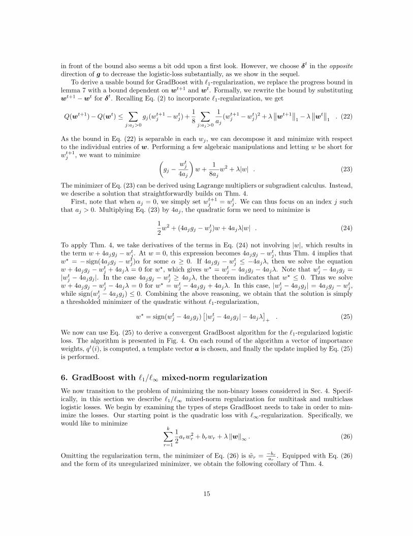
Figure 5: GradBoost for ℓ1/ℓ∞-regularized multitask and multiclass boosting

Adding ℓ∞-regularization terms to Eq. (30), we can upper bound Q(W t+1) − Q(W t) by

Q(W t+1) − Q(W t) ≤∑

j:aj>0

[k∑

r=1

(

gr,j −wt

j,r

2aj

)

wt+1j,r +

1

4

k∑

r=1

(wt+1j,r )2

aj+ λ

∥∥wt+1

j

∥∥∞

−k∑

r=1

gr,jwtj,r +

1

4

k∑

r=1

(wtj,r)

2

aj− λ

∥∥wt

j

∥∥∞

]

. (31)

As was the upper bound for the multitask loss, Eq. (31) is clearly a separable convex quadraticfunction with ℓ∞ regularization for each row wj of W .

We conclude the section with the pseudocode of the unified GradBoost algorithm for the multitaskand the multiclass losses of equations (3) and (4). Note that the upper bounds of Eq. (28) andEq. (31) for both losses are almost identical. The sole difference between the two losses distills tothe definition of the gradient gr,j terms and that in Eq. (31) the constant on aj is half of that inEq. (28). The algorithm is simple: it iteratively calculates the gradient terms gr,j , then employs anupdate template a ∈ A and calls the algorithm of Fig. 2 to minimize Eq. (31). The pseudocode ofthe algorithm is given in Fig. 5.

7. GradBoost with ℓ1/ℓ2 Regularization

One form of regularization that has rarely been considered in the standard boosting literature isℓ2 or ℓ22 regularization. The lack thereof is a consequence of AdaBoost’s exponential bounds onthe decrease in the loss. Concretely, the coupling of the exponential terms with ‖w‖2 or ‖w‖leads to non-trivial minimization problems. GradBoost, however, can straightforwardly incorporateℓ2-based penalties, since it uses linear and quadratic bounds on the decrease in the loss rather

18

than the exponential bounds of AdaBoost. In this section we focus on multiclass GradBoost. Themodification for multitask or standard boosting is straightforward and follows the lines of derivationdiscussed thus far.

We focus particularly on mixed-norm ℓ1/ℓ2-regularization (Obozinski et al., 2007), in which rowsfrom the matrix W = [w1 · · ·wk] are regularized together in an ℓ2-norm. This leads to the followingmodification of the multiclass objective from Eq. (4),

Q(W ) =m∑

i=1

log

1 +∑

r 6=yi

exp(wr · xi − wyi· xi)

+ λn∑

j=1

‖wj‖2 . (32)

Using the bounds from lemma 9 and Eq. (30) and the assumption that∑

i,j ajx2i,j ≤ 1 as before, we

upper bound Q(W t+1) − Q(W t) by

∑

j:aj>0

[k∑

r=1

(

gr,j −wt

j,r

2aj

)

wt+1j,r +

1

4

k∑

r=1

(wt+1j,r )2

aj+ λ

∥∥wt+1

j

∥∥

2+

k∑

r=1

(

(wtj,r)

2

4aj− gr,jw

tj,r

)

− λ∥∥wt

j

∥∥

2

]

(33)The above bound is evidently a separable quadratic function with ℓ2-regularization. We would liketo use Eq. (33) to perform block coordinate descent on the ℓ1/ℓ2-regularized loss Q from Eq. (32).Thus, to minimize the upper bound with respect to wt+1

j,r , we would like to minimize a function ofthe form

1

2a

k∑

r=1

w2r +

k∑

r=1

brwr + λ ‖w‖2 . (34)

The following lemma gives a closed form solution for the minimizer of the above.

Lemma 10 The minimizing w⋆ of Eq. (34) is

w⋆ = −1

a

[

1 − λ

‖b‖2

]

+

b .

Proof We first give conditions under which the solution w⋆ is 0. Characterizing the 0 solution canbe done is several ways. We give here an argument based on the calculus of subgradients (Bertsekas,1999). The subgradient set of λ‖w‖ at w = 0 is the set of vectors z : ‖z‖ ≤ λ. Thus, thesubgradient set of Eq. (34) evaluated at w = 0 is b + z : ‖z‖ ≤ λ, which includes 0 if and onlyif ‖b‖2 ≤ λ. When ‖b‖2 ≤ λ, we clearly have 1 − λ/ ‖b‖2 ≤ 0 which immediately implies that[1 − λ/‖b‖2]+ = 0 and therefore w⋆ = 0 in the statement of the lemma. Next, consider the casewhen ‖b‖2 > λ, so that w⋆ 6= 0 and ∂ ‖w‖2 = w/ ‖w‖2 is well defined. Computing the gradient ofEq. (34) with respect to w, we obtain the optimality condition

aw + b +λ

‖w‖2

w = 0 ⇒(

1 +λ

a ‖w‖2

)

w = −1

ab ,

which implies that w = sb for some s ≤ 0. We next replace the original objective of Eq. (34) with

minimizes

1

2s2

(

ak∑

r=1

b2r

)

+ sk∑

r=1

b2r − λs ‖b‖2 .

Taking the derivative of the objective with respect to s yields,

s a ‖b‖22 + ‖b‖2

2 − λ ‖b‖2 = 0 ⇒ s =λ ‖b‖2 − ‖b‖2

2

a ‖b‖22

=1

a

(λ

‖b‖2

− 1

)

.

19

Input: Training set S = (xi, yi)mi=1;

Regularization λ; number of rounds T ;Update templates A s.t. ∀a ∈ A,

∑

i,j ajx2ij ≤ 1

For t = 1 to TChoose a ∈ AFor j s.t. aj > 0

For i = 1 to m and r = 1 to k// Compute importance weights for each class

Set qt(i, r) = exp(wr·xi)P

kl=1 exp(wl·xi)

For r = 1 to k// Compute gradient termsSet gr,j =

∑mi=1(q

t(i, r) − 1 r = yi)xi,j

gj = [g1,j · · · gk,j ]

wt+1j =

(wt

j − 2ajgj

)[

1 − 2ajλ

‖wtj−2ajgj‖2

]

+

Figure 6: GradBoost for ℓ1/ℓ2-regularized multiclass boosting.

Combining the above result with the case when ‖b‖2 ≤ λ (which yields that w⋆ = 0) while noticingthat λ/ ‖b‖2 − 1 ≤ 0 when ‖b‖2 ≥ λ gives the lemma’s statement.

Returning to Eq. (33), we derive the update to the jth row of W . Defining the gradient vectorgj = [g1,j · · · gr,j ]

⊤ and performing a few algebraic manipulations to Lemma 10, we obtain that theupdate that is performed in order to minimize Eq. (33) with respect to row wj of W is

wt+1j =

(wj − 2ajgj

)

[

1 − 2ajλ∥∥wt

j − 2ajgj

∥∥

2

]

+

. (35)

To recap, we obtain an algorithm for minimizing the ℓ1/ℓ2-regularized multiclass loss by iterativelychoosing update templates a and then applying the update provided in Eq. (35) to each index j forwhich aj > 0. The pseudocode of the algorithm is given in Fig. 6.

8. Learning sparse models by feature induction and pruning

Boosting naturally connotes induction of base hypotheses, or features. Our infusion of regularizationinto boosting and coordinate descent algorithms also facilitates the ability to prune back selectedfeatures. The end result is an algorithmic infrastructure that facilitates forward induction of newfeatures and backward pruning of existing features in the context of an expanded model whileoptimizing weights. In this section we discuss the merits of our paradigm as the means for learningsparse models by introducing and scoring features that have not yet entered a model and pruningback features that are no longer predictive. To do so, we consider the progress bounds we derivedfor AdaBoost and GradBoost. We show how the bounds can provide the means for scoring andselecting new features. We also show that, in addition to scoring features, each of our algorithmsprovides a stopping criterion for inducing new features, indicating feature sets beyond which theintroduction of new hypotheses cannot further decrease the loss. We begin by considering AdaBoostand then revisit the rest of the algorithms and regularizers, finishing the section with a discussionof the boosting termination and hypothesis pruning benefits of our algorithms.

Scoring candidate hypotheses for ℓ1-regularized AdaBoost The analysis in Sec. 2 alsofacilitates assessment of the quality of a candidate weak hypothesis (newly examined feature) during

20

the boosting process. To obtain a bound on the contribution of a new weak hypothesis we plug theform for δt

j from Eq. (8) into the progress bound of Eq. (5). The progress bound can be written asa sum over the progress made by each hypothesis that the chosen template a ∈ A activates. Forconcreteness and overall utility, we focus on the case where we add a single weak hypothesis j. Sincej is as yet un-added, we assume that wj = 0, and as in standard analysis of boosting we assumethat |xi,j | ≤ 1 for all i. Furthermore, for simplicity we assume that aj = 1 and ak = 0 for k 6= j.That is, we revert to the standard boosting process, also known as sequential boosting, in which weadd a new hypothesis on each round. We overload our notation and denote by ∆j the decrease inthe ℓ1-regularized log-loss due to the addition of hypothesis j, and if we define

ν−j =

−λ +√

λ2 + 4µ+j µ−

j

2µ−j

and ν+j =

λ +√

λ2 + 4µ+j µ−

j

2µ−j

,

routine calculations allow us to score a new hypothesis as

∆j =

µ+j + µ−

j − µ+j

ν−

j

− µ−j ν−

j − λ∣∣log ν−

j

∣∣ if µ+

j > µ−j + λ

µ+j + µ−

j − µ+j

ν+j

− µ−j ν+

j − λ∣∣log ν+

j

∣∣ if µ−

j > µ+j + λ

0 if |µ+j − µ−

j | ≤ λ .

(36)

We can thus score candidate weak hypotheses and choose the one with the highest potential to

decrease the loss. Indeed, if we set λ = 0 the decrease in the loss becomes(√

µ+j −

√

µ−j

)2

, which

is the standard boosting progress bound (Collins et al., 2002).

Scoring candidate hypotheses for ℓ1/ℓ∞-regularized AdaBoost Similar arguments to thosefor ℓ1-regularized AdaBoost show that we can assess the quality of a new hypothesis we considerduring the boosting process for mixed-norm AdaBoost. We do not have a closed form for the updateδ that maximizes the bound in the change in the loss from Eq. (17). However, we can solve for theoptimal update for the weights associated with hypothesis j as in Eq. (21) using the algorithm ofFig. 2 and the analysis in Sec. 4. We can plug the resulting updates into the progress bound ofEq. (17) to score candidate hypotheses. The process of scoring hypotheses depends only on thevariables µ±

r,j , which are readily available during the weight update procedure. Thus, the scoringprocess introduces only minor computational burden over the weight update. We also would liketo note that the scoring of hypotheses takes the same form for multiclass and multitask boostingprovided that µ±

r,j have been computed.

Scoring candidate hypotheses for ℓ1-regularized GradBoost It is also possible to derivea scoring mechanism for the induction of new hypotheses in GradBoost by using the lower boundused to derive the GradBoost update. The process of selecting base hypotheses is analogous tothe selection process to get new weak hypotheses for AdaBoost with ℓ1-regularization, which weconsidered above. Recall the quadratic upper bounds on the loss Q(w) from Sec. 5. Since weconsider the addition of new hypotheses, we can assume that wt

j = 0 for all candidate hypotheses.We can thus combine the bound of Eq. (22) and the update of Eq. (25) to obtain

Q(wt) − Q(wt+1) ≥

2aj (|gj | − λ)2 |gj | > λ

0 otherwise .(37)

If we introduce a single new hypothesis at a time, that is, we use an update template a such thataj 6= 0 for a single index j, we can score features individually. To satisfy the constraint that∑

i ajx2i,j ≤ 1, we simply let aj = 1/

∑

i x2i,j . In this case, Eq. (37) becomes

Q(wt) − Q(wt+1) ≥

2(|gj |−λ)2P

mi=1 x2

i,j

|gj | > λ

0 otherwise .

21

Note that the above progress bound incorporates a natural trade-off between the coverage of afeature, as expressed by the term

∑

i x2i,j , and its correlation with the label, expressed through the

difference |gj | = |µ+j − µ−

j |. The larger the difference between µ+j and µ−

j , the higher the potential

of the feature. However, this difference is scaled back by the sum∑

i x2i,j , which is proportional to

the coverage of the feature. A similar though more tacit tension between coverage and correlationis also exhibited in the score for AdaBoost as defined by Eq. (36).

Scoring candidate hypotheses for mixed-norm regularized GradBoost The scoring of newhypotheses for multiclass and multitask GradBoost is similar to that for mixed-norm AdaBoost.The approach for ℓ1/ℓ∞ regularization is analogous to the scoring procedure for AdaBoost. When ahypothesis or feature with index j is being considered for addition on round t, we know that wt

j = 0.We plug the optimal solution of Eq. (28) (or equivalently Eq. (31)), into the progress bound andobtain the potential loss decrease due to the introduction of a new feature. While we cannot providea closed form expression for the potential progress, the complexity of the scoring procedure requiresthe same time as a single feature weight update.

The potential progress does take a closed-form solution when scoring features using ℓ1/ℓ2 mixed-norm regularized GradBoost. We simply plug the update of Eq. (35) into the bound of Eq. (33)while recalling the definition of the gradient terms gj = [g1,j · · · gk,j ]

⊤ for multiclass or multitask

boosting. Since, again, wtj = 0 for a new hypothesis j, a few algebraic manipulations yield that the

progress bound when adding a single new hypothesis j is

Q(W t+1) − Q(W t) ≥

([∥∥gj

∥∥

2− λ

]

+

)2

∑mi=1 x2

i,j

. (38)

Termination Conditions The progress bounds for each of the regularizers also provide us withprincipled conditions for terminating the induction of new hypotheses. We have three differentconditions for termination, depending on whether we use ℓ1, ℓ1/ℓ∞, or ℓ1/ℓ2-regularization. Goingthrough each in turn, we begin with ℓ1. For AdaBoost, Eq. (36) indicates that when |µ+

j −µ−j | ≤ λ,

our algorithm assigns the hypothesis zero weight and no progress can be made. For GradBoost,gj = µ−

j − µ+j , so the termination conditions are identical. In the case of ℓ1/ℓ∞-regularization,

the termination conditions for AdaBoost and Gradboost are likewise identical. For AdaBoost,Corollary 6 indicates that when

∑kr=1 |µ+

r,j −µ−r,j | ≤ λ the addition of hypothesis j cannot decrease.

Analogously for GradBoost, Corollary 8 shows that when∑k

r=1 |gr,j | ≤ λ then wt+1j = 0, which is

identical since gr,j = µ−r,j −µ+

r,j . For ℓ1/ℓ2-regularized GradBoost, examination of Eq. (38) indicates

that if∥∥gj

∥∥

2≤ λ, then adding hypothesis j does not decrease the loss.

As we discuss in the next section, each of our algorithms converges to the optimum of its respectiveloss. Therefore, assume we have learned a model with a set of features such that the feature weightsare at the optimum for the regularized loss (using only the current features in the model) we areminimizing. The convergence properties indicate that if our algorithm cannot make progress usingthe jth hypothesis, then truly no algorithm that uses the jth hypothesis in conjunction with thecurrent model can make progress on the objective. The same property holds even in the case ofan infinite hypothesis space. We thus see that each algorithm gives a condition for terminatingboosting. Specifically, we know when we have exhausted the space of base hypotheses that cancontribute to a reduction in the regularized loss.

Backpruning In addition to facilitating simple scoring mechanisms, the updates presented forAdaBoost and GradBoost in the various settings also enable resetting the weight of a hypothesisif in retrospect (after further boosting rounds) its predictive power decreases. Take for examplethe ℓ1-penalized boosting steps of AdaBoost. When the weight-adjusted difference between µ+

j and

µ−j in the AdaBoost algorithm in Fig. 1 falls below λ, that is,

∣∣∣µ+

j ewtj/aj − µ−

j e−wtj/aj

∣∣∣ ≤ λ, we

22

set δtj = −wt

j and we zero out the jth weight. Thus, the ℓ1-penalized boosting steps enable bothinduction of new hypotheses along with backward pruning of previously selected hypotheses. Similarstatements apply to all of our algorithms, namely, when weight-adjusted correlations or gradientsfall below the regularization, the algorithms can zero weights or rows of weights.

As mentioned in the introduction, we can also alternate between pure weight updates (restrictingourselves to the current set of hypotheses) and pure induction of new hypotheses (keeping the weightof existing hypotheses intact). As demonstrated empirically in our experiments, the end result ofboosting with the sparsity promoting ℓ1, ℓ1/ℓ2, or ℓ1/ℓ∞-regularizers is a compact and accuratemodel. This approach of alternating weight optimization and hypothesis induction is also reminiscentof the recently suggested forward-backward greedy process for learning sparse representations inleast-squares models (Zhang, 2008). However, in our setting the backward pruning is not performedin a greedy manner but is rather driven by the non-differentiable convex regularization penalties.

Template Selection Finally, the templating of our algorithms allows us to make the templatesa application and data dependent. If the computing environment consists of a few uncoupledprocessors and the features are implicit (e.g. boosted decision trees), then the most appropriateset of templates is the set of singleton vectors (we get the best progress guarantee from the highestscoring singletons). When the features are explicit and the data is rather sparse, i.e.

∑

j |xi,j | ≪ n

where xi,j is the prediction of the jth base hypothesis on the ith example, we can do better byletting the templates be dense. For example, for ℓ1-regularized AdaBoost, we can use a singletemplate vector a with aj = 1/maxi

∑

j |xi,j | for all j. For GradBoost, we can use the single

template a with that aj = 1/(n∑m

i=1 x2i,j

). Dense templates are particularly effective in parallel

computing environments where we can efficiently compute importance-weighted correlations µ+j and

µ−j or gradients gr,j for all possible features. We can then make progress simultaneously for multiple

features and use the full parallelism available.

9. Convergence properties

We presented several variants for boosting-based stepping with different regularized logistic lossesthroughout this paper. To conclude the formal part of the paper, we discuss the convergence prop-erties of these algorithms. Each of our algorithms is guaranteed to converge to an optimum of itsrespective loss, provided that the weight of each feature is examined and potentially updated suffi-ciently often. We thus discuss jointly the convergence of all the algorithms. Concretely, when thenumber of hypotheses is finite, the boosting updates for both the AdaBoost and GradBoost algo-rithms are guaranteed to converge under realistic conditions. The conditions require the templatesa ∈ A to span the entire space, assume that there are a finite number of hypotheses, and eachhypothesis is updated infinitely often. The optimal weights of the (finitely many) induced featurescan then be found using a set of templates that touch each of the features. In particular, a singletemplate that updates the weight of all of the features simultaneously can be used, as could a setof templates that iteratively selects one feature at a time. The following theorem summarizes theconvergence properties. Due to its technical nature we provide its proof in Appendix C. The proofrelies on the fact that the regularization term forces the set of possible solutions of any of the regu-larized losses we discuss to be compact. In addition, each of the updates guarantees some decrease inits respective regularized loss. Roughly, each sequence of weights obtained by any of the algorithmstherefore converges to a stationary point guaranteed to be the unique optimum by convexity. Weare as yet unable to derive rates of convergence for our algorithms, but we hope that recent viewsof boosting processes as primal-dual games (Schapire, 1999; Shalev-Shwartz and Singer, 2008) oranalysis of randomized coordinate descent algorithms (Shalev-Shwartz and Tewari, 2009) can helpin deriving more refined results.

23

Theorem 11 Assume that the number of hypotheses is finite and each hypothesis participates in anupdate based on either AdaBoost or GradBoost infinitely often. Then all the variants of regularizedboosting algorithms converge to the optimum of their respective objectives. Specifically,

i. AdaBoost with ℓ1-regularization converges to the optimum of Eq. (2).

ii. Multitask and Multiclass AdaBoost with ℓ1/ℓ∞-regularization converge to the optimum of Eq. (3)and Eq. (4), respectively.

iii. GradBoost with ℓ1-regularization convergences to the optimum of Eq. (2).

iv. Multitask and Multiclass GradBoost with ℓ1/ℓ∞-regularization converge to the optimum of Eq. (3)and Eq. (4), respectively.

v. GradBoost with ℓ1/ℓ2-regularization converges to the optimum of Eq. (32).

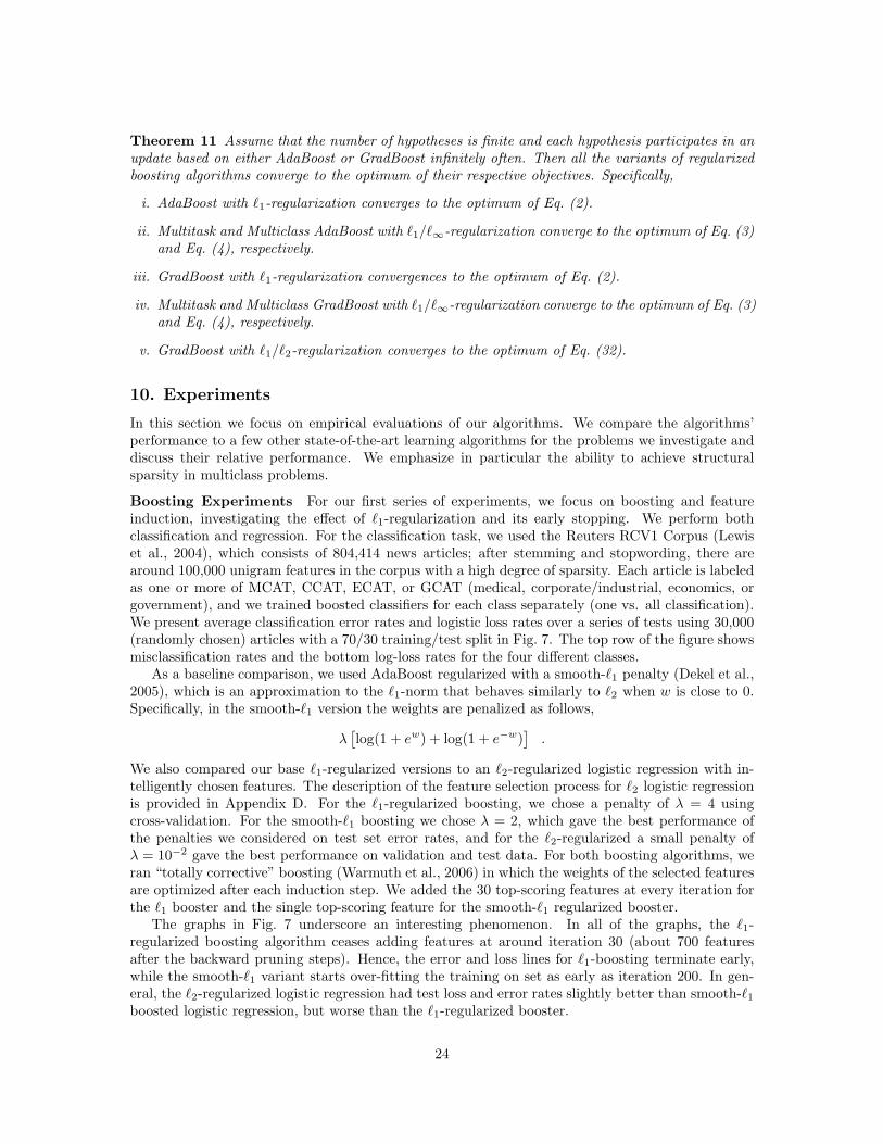
10. Experiments

In this section we focus on empirical evaluations of our algorithms. We compare the algorithms’performance to a few other state-of-the-art learning algorithms for the problems we investigate anddiscuss their relative performance. We emphasize in particular the ability to achieve structuralsparsity in multiclass problems.

Boosting Experiments For our first series of experiments, we focus on boosting and featureinduction, investigating the effect of ℓ1-regularization and its early stopping. We perform bothclassification and regression. For the classification task, we used the Reuters RCV1 Corpus (Lewiset al., 2004), which consists of 804,414 news articles; after stemming and stopwording, there arearound 100,000 unigram features in the corpus with a high degree of sparsity. Each article is labeledas one or more of MCAT, CCAT, ECAT, or GCAT (medical, corporate/industrial, economics, orgovernment), and we trained boosted classifiers for each class separately (one vs. all classification).We present average classification error rates and logistic loss rates over a series of tests using 30,000(randomly chosen) articles with a 70/30 training/test split in Fig. 7. The top row of the figure showsmisclassification rates and the bottom log-loss rates for the four different classes.

As a baseline comparison, we used AdaBoost regularized with a smooth-ℓ1 penalty (Dekel et al.,2005), which is an approximation to the ℓ1-norm that behaves similarly to ℓ2 when w is close to 0.Specifically, in the smooth-ℓ1 version the weights are penalized as follows,

λ[log(1 + ew) + log(1 + e−w)

].

We also compared our base ℓ1-regularized versions to an ℓ2-regularized logistic regression with in-telligently chosen features. The description of the feature selection process for ℓ2 logistic regressionis provided in Appendix D. For the ℓ1-regularized boosting, we chose a penalty of λ = 4 usingcross-validation. For the smooth-ℓ1 boosting we chose λ = 2, which gave the best performance ofthe penalties we considered on test set error rates, and for the ℓ2-regularized a small penalty ofλ = 10−2 gave the best performance on validation and test data. For both boosting algorithms, weran “totally corrective” boosting (Warmuth et al., 2006) in which the weights of the selected featuresare optimized after each induction step. We added the 30 top-scoring features at every iteration forthe ℓ1 booster and the single top-scoring feature for the smooth-ℓ1 regularized booster.

The graphs in Fig. 7 underscore an interesting phenomenon. In all of the graphs, the ℓ1-regularized boosting algorithm ceases adding features at around iteration 30 (about 700 featuresafter the backward pruning steps). Hence, the error and loss lines for ℓ1-boosting terminate early,while the smooth-ℓ1 variant starts over-fitting the training on set as early as iteration 200. In gen-eral, the ℓ2-regularized logistic regression had test loss and error rates slightly better than smooth-ℓ1boosted logistic regression, but worse than the ℓ1-regularized booster.

24

100 200 300 400 500 600 700 800

0.02

0.03

0.04

0.05

0.06

0.07

0.08

0.09

0.1

0.11

MCAT Error Rates

Smooth−trainSmooth−testL1−trainL1−testL2−test

100 200 300 400 500 600 700 800

0.06

0.08

0.1

0.12

0.14

0.16

0.18

CCAT Error Rates

100 200 300 400 500 600 700 8000.02

0.03

0.04

0.05

0.06

0.07

0.08

0.09

ECAT Error Rates

100 200 300 400 500 600 700 800

0.02

0.03

0.04

0.05

0.06

0.07

0.08

0.09

GCAT Error Rates

100 200 300 400 500 600 700 800

0.1

0.15

0.2

0.25

MCAT Loss Rates

Smooth−trainSmooth−testL1−trainL1−testL2−test

100 200 300 400 500 600 700 800

0.15

0.2

0.25

0.3

0.35

0.4

CCAT Loss Rates

100 200 300 400 500 600 700 800

0.08

0.1

0.12

0.14

0.16

0.18

0.2

0.22

0.24

ECAT Loss Rates

100 200 300 400 500 600 700 800

0.06

0.08

0.1

0.12

0.14

0.16

0.18

0.2

0.22

0.24

GCAT Loss Rates

Figure 7: Error rates and losses on the Reutes corpus for various boosting-based algorithms. Thelegend is the same for all graphs.

We also conducted various regression experiments. We describe here the results obtained forthe Boston housing data set from the UCI repository (Asuncion and Newman, 2007) and a dataseton controlling an F16 aircraft, where the goal is to predict a control action on the ailerons of theaircraft given its state (Camacho, 1997). We standardized both datasets so that their variablesare all in the range [0, 1] (for housing) or [−1, 1] (for ailerons). We then used boosted ε-insensitiveregression (Dekel et al., 2005) to learn a predictor w. In this case, our objective is

m∑

i=1

log(1 + ew·xi−yi−ε

)+ log

(1 + eyi−w·xi−ε

), (39)

which approximates ε-insensitive hinge regression [w · xi − yi − ε]+ + [yi − w · xi − ε]+ where[x]+ = maxx, 0. For ε-insensitive regression, an analysis similar to that for standard boostingcan be performed to compute µ+ and µ− for every feature (see appendix section A), which allowsus to perform scoring during feature induction and to take update steps identical to those alreadydescribed.

For these tests, we compared the unregularized “classical” sequential AdaBoost, ℓ1-regularizedtotally corrective boosting with induction of eight top-scoring features at the end of each optimizationstep, ℓ1-regularized least squares (Friedman et al., 2007), and ℓ2-regularized ε-insensitive hingeloss. The boosters used a countably infinite set of features by examining products of features. Allalgorithms were started with a single bias feature. Thus, the algorithms could construct arbitrarilymany products of raw features as base (weak) hypotheses and explore complex correlations betweenthe features. For ℓ1-regularized least squares, we simply trained on the base regressors, and forℓ2-regularized hinge loss we trained on the base regressors using projected subgradient methodsdescribed in Shalev-Shwartz et al. (2007).

Fig. 8 illustrates the results of these experiments. The housing results are the left pair of graphswhile aileron results are the right. The left plot of each pair provides the root-mean-square error onthe test set, and the right of the pair the average absolute error on the test sets. In all experiments,we set λ = .02 for the ℓ1-penalty, and the ℓ1-regularized booster stopped after inducing an average ofunder 35 features. The last iteration of the ℓ1-regularized version is marked with a star in the graphs,after which a dotted line indicates the resulting performance. We see that even when the sequential(denoted Classical) boosting is allowed to run for 1000 iterations, its performance on test does notmeet the performance obtained by the 35 feature ℓ1-regularized model. As a further experiment,we allowed the sequential boosting process to run for 3000 iterations, yet still its performance did

25

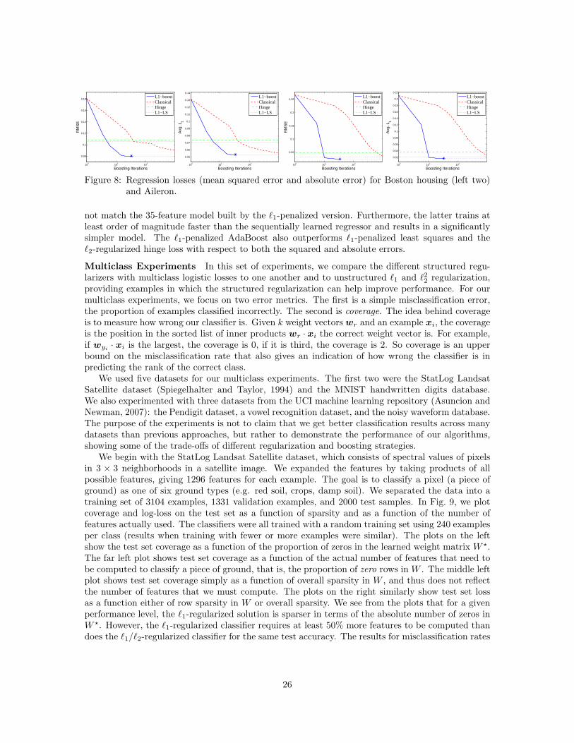
100

101

102

0.08

0.1

0.12

0.14

0.16

0.18

Boosting Iterations

RM

SE

L1−boostClassicalHingeL1−LS

100

101

102

0.05

0.06

0.07

0.08

0.09

0.1

0.11

0.12

0.13

0.14

Boosting Iterations

Avg

. L1

L1−boostClassicalHingeL1−LS

100

101

102

0.05

0.1

0.15

0.2

0.25

Boosting Iterations

RM

SE

L1−boostClassicalHingeL1−LS

100

101

102

0.02

0.04

0.06

0.08

0.1

0.12

0.14

0.16

0.18

0.2

0.22

Boosting Iterations

Avg

. L1

L1−boostClassicalHingeL1−LS

Figure 8: Regression losses (mean squared error and absolute error) for Boston housing (left two)and Aileron.

not match the 35-feature model built by the ℓ1-penalized version. Furthermore, the latter trains atleast order of magnitude faster than the sequentially learned regressor and results in a significantlysimpler model. The ℓ1-penalized AdaBoost also outperforms ℓ1-penalized least squares and theℓ2-regularized hinge loss with respect to both the squared and absolute errors.

Multiclass Experiments In this set of experiments, we compare the different structured regu-larizers with multiclass logistic losses to one another and to unstructured ℓ1 and ℓ22 regularization,providing examples in which the structured regularization can help improve performance. For ourmulticlass experiments, we focus on two error metrics. The first is a simple misclassification error,the proportion of examples classified incorrectly. The second is coverage. The idea behind coverageis to measure how wrong our classifier is. Given k weight vectors wr and an example xi, the coverageis the position in the sorted list of inner products wr · xi the correct weight vector is. For example,if wyi

· xi is the largest, the coverage is 0, if it is third, the coverage is 2. So coverage is an upperbound on the misclassification rate that also gives an indication of how wrong the classifier is inpredicting the rank of the correct class.

We used five datasets for our multiclass experiments. The first two were the StatLog LandsatSatellite dataset (Spiegelhalter and Taylor, 1994) and the MNIST handwritten digits database.We also experimented with three datasets from the UCI machine learning repository (Asuncion andNewman, 2007): the Pendigit dataset, a vowel recognition dataset, and the noisy waveform database.The purpose of the experiments is not to claim that we get better classification results across manydatasets than previous approaches, but rather to demonstrate the performance of our algorithms,showing some of the trade-offs of different regularization and boosting strategies.

We begin with the StatLog Landsat Satellite dataset, which consists of spectral values of pixelsin 3 × 3 neighborhoods in a satellite image. We expanded the features by taking products of allpossible features, giving 1296 features for each example. The goal is to classify a pixel (a piece ofground) as one of six ground types (e.g. red soil, crops, damp soil). We separated the data into atraining set of 3104 examples, 1331 validation examples, and 2000 test samples. In Fig. 9, we plotcoverage and log-loss on the test set as a function of sparsity and as a function of the number offeatures actually used. The classifiers were all trained with a random training set using 240 examplesper class (results when training with fewer or more examples were similar). The plots on the leftshow the test set coverage as a function of the proportion of zeros in the learned weight matrix W ⋆.The far left plot shows test set coverage as a function of the actual number of features that need tobe computed to classify a piece of ground, that is, the proportion of zero rows in W . The middle leftplot shows test set coverage simply as a function of overall sparsity in W , and thus does not reflectthe number of features that we must compute. The plots on the right similarly show test set lossas a function either of row sparsity in W or overall sparsity. We see from the plots that for a givenperformance level, the ℓ1-regularized solution is sparser in terms of the absolute number of zeros inW ⋆. However, the ℓ1-regularized classifier requires at least 50% more features to be computed thandoes the ℓ1/ℓ2-regularized classifier for the same test accuracy. The results for misclassification rates

26

0 0.05 0.1 0.15 0.2 0.250.2

0.3

0.4

0.5

0.6

0.7

0.8

Cov

erag

e

Proportion features used

L1L1/L2L1/Linf

0 0.05 0.1 0.15 0.2 0.25

0.2

0.3

0.4

0.5

0.6

0.7

0.8

Cov

erag

e

Proportion nonzero

0.1 0.2 0.3 0.4 0.5 0.6 0.7

550

600

650

700

750

800

850

900

950

1000

Tes

t los

s

Proportion features used

0.1 0.2 0.3 0.4 0.5 0.6 0.7

550

600

650

700

750

800

850

900

950

Tes

t los

s

Proportion nonzero

Figure 9: LandSat test coverage and losses. Far left: coverage versus row sparsity. Middle left:coverage versus overall sparsity. Middle right: test loss versus row sparsity. Far right: testloss versus overall sparsity.

0.2 0.3 0.4 0.5 0.6 0.7 0.81

1.2

1.4

1.6

1.8

2

2.2

Cov

erag

e

Proportion features used

L1L1/L2L1/Linf

0.2 0.3 0.4 0.5 0.6 0.7 0.81

1.1

1.2

1.3

1.4

1.5

1.6

1.7

1.8

1.9

2

Cov

erag

e

Proportion nonzero

0.1 0.2 0.3 0.4 0.5 0.6 0.7 0.8600

700

800

900

1000

1100

1200

1300

1400

1500

Tes

t los

s

Proportion features used

0.1 0.2 0.3 0.4 0.5 0.6 0.7 0.8600

700

800

900

1000

1100

1200

1300

1400

1500

1600

Tes

t los

s

Proportion nonzero

Figure 10: Vowels test coverage and losses. Far left: coverage versus row sparsity. Middle left:coverage versus overall sparsity. Middle right: test loss versus row sparsity. Far right:test loss versus overall sparsity.

0.2 0.3 0.4 0.5 0.6 0.7 0.8 0.9 10

0.05

0.1

0.15

0.2

0.25

0.3

0.35

0.4

Cov

erag

e

Proportion features used

L1L1/L2L1/Linf

0.1 0.2 0.3 0.4 0.5 0.6 0.7 0.8 0.9 10

0.05

0.1

0.15

0.2

0.25

0.3

0.35

0.4

Cov

erag

e

Proportion nonzero

0.2 0.3 0.4 0.5 0.6 0.7 0.8 0.9 1500

1000

1500

2000

2500

3000

Tes

t los

s

Proportion features used

L1L1/L2L1/Linf

0.1 0.2 0.3 0.4 0.5 0.6 0.7 0.8 0.9 1

600

800

1000

1200

1400

1600

1800

2000

2200

2400

2600

2800T

est l

oss

Proportion nonzero

L1L1/L2L1/Linf

Figure 11: Pendigit handwritten digits test coverage and losses. Far left: coverage versus row spar-sity. Middle left: coverage versus overall sparsity. Middle right: test loss versus rowsparsity. Far right: test loss versus overall sparsity.

0.1 0.2 0.3 0.4 0.5 0.6 0.7 0.8 0.9 1

0.13

0.135

0.14

0.145

0.15

0.155

0.16

0.165

Cov

erag

e

Proportion features used

L1L1/L2L1/Linf

0 0.1 0.2 0.3 0.4 0.5 0.6 0.7 0.8 0.9 1

0.13

0.135

0.14

0.145

0.15

0.155

0.16

Cov

erag

e

Proportion nonzero

0 0.1 0.2 0.3 0.4 0.5 0.6 0.7 0.8 0.9

800

850

900

950

1000

1050

1100

Tes

t los

s

Proportion features used

0.1 0.2 0.3 0.4 0.5 0.6 0.7 0.8 0.9

800

850

900

950

1000

Tes

t los

s

Proportion nonzero

Figure 12: Waveform test coverage and losses. Far left: coverage versus row sparsity. Middle left:coverage versus overall sparsity. Middle right: test loss versus row sparsity. Far right:test loss versus overall sparsity.

27

are similar. We computed these results over ten randomly chosen subsets of the training data andthe variance of each point in the plot is smaller than 10−3.

In figures 10, 11, and 12, we plot the results obtained on the remaining UCI datasets. Thevowel experiments require classifying a vowel spoken in the middle of a word as one of 11 differentvowels. We expanded the original 10 features by taking products of all features. We trained with 20training examples per class (results are similar using 40 examples per class) over 10 different randomtraining runs. We plot test set coverage and loss as a function of sparsity in Fig. 10. In the Pendigitexperiments we classify a handwritten digit, with 16 features recorded from a pressure-sensitivestylus, as one of 10 different digits. Again we expanded into products of features, and in Fig. 11 weplot loss and coverage for this task versus sparsity in the solution matrix W . We trained with 300examples per class (as with our other experiments, results were similar across training set sizes) andused a test set of 3498 examples. The last UCI dataset we consider was the Waveform dataset, asynthetic 3 class problem where the goal is to classify different randomly generated waves. Originallyconsisting of 40 attributes, we expanded the feature space using products of feature and created 820features. We then applied our multiclass boosting algorithms. We used a test set of 2500 examplesand training set of 600 examples per class. We plot our test loss and coverage results versus sparsityin W in Fig. 12. We repeated each of our UCI experiments over 10 randomly sub-selected trainingsets. Each of the plots in figures 10 and 11 exhibits results similar to the results obtained for theLandsat dataset. Examining the performance as a function of the actual number of features thatmust be computed, ℓ1/ℓ2 and ℓ1/ℓ∞ regularizations seem to yield better performance, while if weare mainly concerned with overall sparsity of the learned matrix W , ℓ1-regularization gives betterperformance. For the Waveform dataset (Fig. 12), it seems that performance was similar acrossall the regularizers, which may be an artifact of the waveforms being synthetic, with performanceimproving as the number of features used got very small.

We also conducted experiments using the MNIST handwritten digits database. The MNISTdataset consists of 60,000 training examples and a 10,000 example test set and has 10-classes. Eachimage is a gray-scale 28 × 28 matrix, which we represent as vector xi ∈ R

784. Rather than directlyusing the input xi, we learned weights wj for Kernel-based weak-hypotheses

hj(x) = K(xj ,x), K(x,z) = e−12‖x−z‖2

,

for j ∈ S, where S is a 2766 element support set. We generated the support set by running the Per-ceptron algorithm once through the dataset while keeping examples on which it made classificationmistakes. We obtained this way a 27,660 dimensional multiclass problem to which we apply ouralgorithms. On the left side of Fig. 13, we plot the coverage on the 10,000 example test set of eachalgorithm versus the number of training examples used per class. We chose regularization valuesusing cross-validation. The performance improves as the number of training examples increases.However, it is clear that the sparsity promoting regularizers, specifically the structural ℓ1/ℓ∞ andℓ1/ℓ2 regularizers, yield better performance than the others. The error rate on the test set is roughlyhalf the coverage value and behaves qualitatively similar.

To conclude this section we would like to attempt to provide a few insights into the relative meritsof AdaBoost versus GradBoost when both can be applied, namely, for ℓ1 and ℓ1/ℓ∞-regularizedproblems. On the right side of Fig. 13, we plot the training objective as a function of trainingtime for both AdaBoost and GradBoost on the Landsat and MNIST datasets. On the same timescale, we plot the test error rate and sparsity of the classifiers as a function of training time inFig. 14 (in the left and right plots, respectively). From Fig. 14, we see that both AdaBoost andGradBoost indeed leverage induction during the first few thousand iterations, adding many featuresthat contribute to decreasing the loss. They then switch to a backward-pruning phase in which theyremove features that are not predictive enough without increasing the loss on the test set. We sawsimilar behavior across many datasets, which underscores the ability of the algorithms to performboth feature induction and backward pruning in tandem.

28

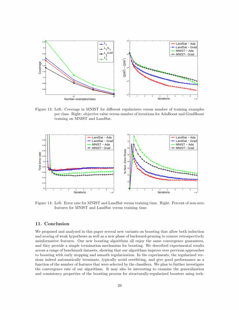
102

103

0.06

0.08

0.1

0.12

0.14

0.16

0.18

0.2

0.22

Number examples/class

Cov

erag

e

L1

L1/L

2

L1/Linf

L22

0 1 2 3 4 5 6 7 8 9

x 104

100

101

102

103

104

Iterations

Q(W

t ) −

Q(W

* )

LandSat − AdaLandSat − GradMNIST − AdaMNIST− Grad

Figure 13: Left: Coverage in MNIST for different regularizers versus number of training examplesper class. Right: objective value versus number of iterations for AdaBoost and GradBoosttraining on MNIST and LandSat.

0 1 2 3 4 5 6 7 8 9

x 104

0.1

0.12

0.14

0.16

0.18

0.2

0.22

0.24

0.26

0.28

Iterations

Tes

t err

or r

ate

LandSat − AdaLandSat − GradMNIST − AdaMNIST− Grad

0 1 2 3 4 5 6 7 8 9

x 104

0

10

20

30

40

50

60

70

80

Iterations

% N

on−

Zer

o R

ows

LandSat − AdaLandSat − GradMNIST − AdaMNIST− Grad

Figure 14: Left: Error rate for MNIST and LandSat versus training time. Right: Percent of non-zerofeatures for MNIST and LandSat versus training time.

11. Conclusion

We proposed and analyzed in this paper several new variants on boosting that allow both inductionand scoring of weak hypotheses as well as a new phase of backward-pruning to remove retrospectivelyuninformative features. Our new boosting algorithms all enjoy the same convergence guarantees,and they provide a simple termination mechanism for boosting. We described experimental resultsacross a range of benchmark datasets, showing that our algorithms improve over previous approachesto boosting with early stopping and smooth regularization. In the experiments, the regularized ver-sions indeed automatically terminate, typically avoid overfitting, and give good performance as afunction of the number of features that were selected by the classifiers. We plan to further investigatethe convergence rate of our algorithms. It may also be interesting to examine the generalizationand consistency properties of the boosting process for structurally-regularized boosters using tech-

29

niques from Schapire et al. (1998) or Zhang and Yu (2005) and other techniques for analyzing thegeneralization properties of boosting.

Acknowledgements

A substantial part of the work of J. Duchi was performed at Google. We would like to thank ShaiShalev-Shwartz for useful discussions.

References

A. Asuncion and D. J. Newman. UCI machine learning repository, 2007. URLhttp://www.ics.uci.edu/∼mlearn/MLRepository.html.

D.P. Bertsekas. Nonlinear Programming. Athena Scientific, 1999.

S. Boyd and L. Vandenberghe. Convex Optimization. Cambridge University Press, 2004.

Rui Camacho. Ailerons dataset. URL http://www.liaad.up.pt/ ltorgo/Regression/DataSets.html.Available at http://www.liaad.up.pt/˜ltorgo/Regression/DataSets.html, 1997.

M. Collins, R.E. Schapire, and Y. Singer. Logistic regression, AdaBoost and Bregman distances.Machine Learning, 47(2/3):253–285, 2002.

O. Dekel, S. Shalev-Shwartz, and Y. Singer. Smooth epsilon-insensitive regression by loss sym-metrization. Journal of Machine Learning Research, 6:711–741, May 2005.

J. Duchi, S. Shalev-Shwartz, Y. Singer, and T. Chandra. Efficient projections onto the ℓ1-ball forlearning in high dimensions. In Proceedings of the 25th International Conference on MachineLearning, 2008.

M. Dudık, S. J. Phillips, and R. E. Schapire. Maximum entropy density estimation with generalizedregularization and an application to species distribution modeling. Journal of Machine LearningResearch, 8:1217–1260, June 2007.

T. Evgeniou, C.Micchelli, and M. Pontil. Learning multiple tasks with kernel methods. Journal ofMachine Learning Research, 6:615–637, 2005.

Y. Freund and R.E. Schapire. A decision-theoretic generalization of on-line learning and an appli-cation to boosting. Journal of Computer and System Sciences, 55(1):119–139, August 1997.

J. Friedman, T. Hastie, and R. Tibshirani. Additive logistic regression: a statistical view of boosting.Annals of Statistics, 28(2):337–374, April 2000.

Jerome Friedman, Trevor Hastie, and Robert Tibshirani. Pathwise coordinate optimization. Annalsof Applied Statistics, 1(2):302–332, 2007.

Roger A. Horn and Charles R. Johnson. Matrix Analysis. Cambridge University Press, 1985.

L. Jacob, F. Bach, and J.-P. Vert. Clustered multi-task learning: A convex formulation. In Advancesin Neural Information Processing Systems 22, 2008.

K. Koh, S.J. Kim, and S. Boyd. An interior-point method for large-scale ℓ1-regularized logisticregression. Journal of Machine Learning Research, 8:1519–1555, 2007.

S. I. Lee, H. Lee, P. Abbeel, and A. Y. Ng. Efficient ℓ1-regularized logistic regression. In ProceedingsAAAI-06. American Association for Artificial Intelligence, 2006.

30

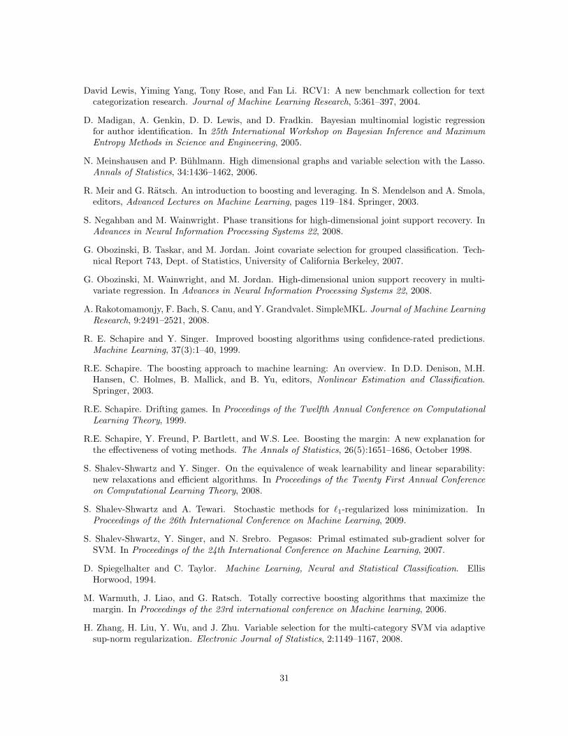
David Lewis, Yiming Yang, Tony Rose, and Fan Li. RCV1: A new benchmark collection for textcategorization research. Journal of Machine Learning Research, 5:361–397, 2004.

D. Madigan, A. Genkin, D. D. Lewis, and D. Fradkin. Bayesian multinomial logistic regressionfor author identification. In 25th International Workshop on Bayesian Inference and MaximumEntropy Methods in Science and Engineering, 2005.

N. Meinshausen and P. Buhlmann. High dimensional graphs and variable selection with the Lasso.Annals of Statistics, 34:1436–1462, 2006.

R. Meir and G. Ratsch. An introduction to boosting and leveraging. In S. Mendelson and A. Smola,editors, Advanced Lectures on Machine Learning, pages 119–184. Springer, 2003.

S. Negahban and M. Wainwright. Phase transitions for high-dimensional joint support recovery. InAdvances in Neural Information Processing Systems 22, 2008.

G. Obozinski, B. Taskar, and M. Jordan. Joint covariate selection for grouped classification. Tech-nical Report 743, Dept. of Statistics, University of California Berkeley, 2007.

G. Obozinski, M. Wainwright, and M. Jordan. High-dimensional union support recovery in multi-variate regression. In Advances in Neural Information Processing Systems 22, 2008.

A. Rakotomamonjy, F. Bach, S. Canu, and Y. Grandvalet. SimpleMKL. Journal of Machine LearningResearch, 9:2491–2521, 2008.

R. E. Schapire and Y. Singer. Improved boosting algorithms using confidence-rated predictions.Machine Learning, 37(3):1–40, 1999.

R.E. Schapire. The boosting approach to machine learning: An overview. In D.D. Denison, M.H.Hansen, C. Holmes, B. Mallick, and B. Yu, editors, Nonlinear Estimation and Classification.Springer, 2003.

R.E. Schapire. Drifting games. In Proceedings of the Twelfth Annual Conference on ComputationalLearning Theory, 1999.

R.E. Schapire, Y. Freund, P. Bartlett, and W.S. Lee. Boosting the margin: A new explanation forthe effectiveness of voting methods. The Annals of Statistics, 26(5):1651–1686, October 1998.

S. Shalev-Shwartz and Y. Singer. On the equivalence of weak learnability and linear separability:new relaxations and efficient algorithms. In Proceedings of the Twenty First Annual Conferenceon Computational Learning Theory, 2008.

S. Shalev-Shwartz and A. Tewari. Stochastic methods for ℓ1-regularized loss minimization. InProceedings of the 26th International Conference on Machine Learning, 2009.

S. Shalev-Shwartz, Y. Singer, and N. Srebro. Pegasos: Primal estimated sub-gradient solver forSVM. In Proceedings of the 24th International Conference on Machine Learning, 2007.

D. Spiegelhalter and C. Taylor. Machine Learning, Neural and Statistical Classification. EllisHorwood, 1994.

M. Warmuth, J. Liao, and G. Ratsch. Totally corrective boosting algorithms that maximize themargin. In Proceedings of the 23rd international conference on Machine learning, 2006.

H. Zhang, H. Liu, Y. Wu, and J. Zhu. Variable selection for the multi-category SVM via adaptivesup-norm regularization. Electronic Journal of Statistics, 2:1149–1167, 2008.

31

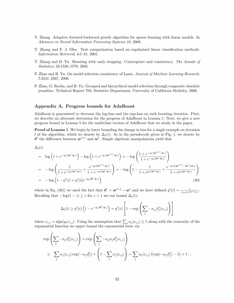
T. Zhang. Adaptive forward-backward greedy algorithm for sparse learning with linear models. InAdvances in Neural Information Processing Systems 22, 2008.

T. Zhang and F. J. Oles. Text categorization based on regularized linear classification methods.Information Retrieval, 4:5–31, 2001.

T. Zhang and B. Yu. Boosting with early stopping: Convergence and consistency. The Annals ofStatistics, 33:1538–1579, 2005.

P. Zhao and B. Yu. On model selection consistency of Lasso. Journal of Machine Learning Research,7:2541–2567, 2006.

P. Zhao, G. Rocha, and B. Yu. Grouped and hierarchical model selection through composite absolutepenalties. Technical Report 703, Statistics Department, University of California Berkeley, 2006.

Appendix A. Progress bounds for AdaBoost

AdaBoost is guaranteed to decrease the log-loss and the exp-loss on each boosting iteration. First,we describe an alternate derivation for the progress of AdaBoost in Lemma 1. Next, we give a newprogress bound in Lemma 5 for the multiclass version of AdaBoost that we study in the paper.

Proof of Lemma 1 We begin by lower bounding the change in loss for a single example on iterationt of the algorithm, which we denote by ∆t(i). As in the pseudocode given in Fig. 1, we denote byδt the difference between wt+1 and wt. Simple algebraic manipulations yield that

∆t(i)

= log(

1 + e−yi(wt·xi)

)

− log(

1 + e−yi(wt+1·xi)

)

= − log

(

1 + e−yi(wt+1·xi)

1 + e−yi(wt·xi)

)

= − log

(

1

1 + e−yi(wt·xi)+

e−yi(wt+1·xi)

1 + e−yi(wt·xi)

)

= − log

(

1 − 1

1 + eyi(wt·xi)+

e−yi((wt+1−wt)·xi)

1 + eyi(wt·xi)

)

= − log(

1 − qt(i) + qt(i)e−yi(δt·xi)

)

(40)

where in Eq. (40)) we used the fact that δt = wt+1 − wt and we have defined qt(i) = 1

1+eyi(wt·xi)

.

Recalling that − log(1 − z) ≥ z for z < 1 we can bound ∆t(i):

∆t(i) ≥ qt(i)(

1 − e−yi(δt·xi)

)

= qt(i)

1 − exp

∑

j

−si,jδtj |xi,j |

where si,j = sign(yixi,j). Using the assumption that∑

j aj |xi,j | ≤ 1 along with the convexity of theexponential function we upper bound the exponential term via

exp

∑

j

−sijδtj |xi,j |

= exp

∑

j

−sijajdtj |xi,j |

≤∑

j

aj |xi,j | exp(−sijdtj) +

1 −∑

j

aj |xi,j |

=∑

j

aj |xi,j |(exp(−sijd

tj) − 1

)+ 1 ,

32

where δtj = ajd

tj . We thus obtain that

∆t(i) ≥ qt(i)

∑

j

aj |xi,j |(

1 − e−sijdtj

)

.

Summing over all our training examples, we get

∆t =

m∑

i=1

∆t(i) ≥m∑

i=1

qt(i)

∑

j

aj |xi,j |(

1 − e−sijdtj

)

=

n∑

j=1

aj

m∑

i=1

qt(i)|xi,j |(

1 − e−sijdtj

)

=

n∑

j=1

aj

∑

i:yixi,j>0

qt(i)|xi,j |(

1 − e−dtj

)

+∑

i:yixi,j<0

qt(i)|xi,j |(

1 − edtj

)

=n∑

j=1

aj

(

µ+j

(

1 − e−dtj

)

+ µ−j

(

1 − edtj

))

, (41)

where in Eq. (41) we use the definitions of µ+j and µ−

j ,

µ+j =

∑

i:yixi,j>0

qt(i)|xi,j | and µ−j =

∑

i:yixi,j<0

qt(i)|xi,j | .

Finally, replacing dtj with δt

j/aj , we get

∆t ≥n∑

j=1

aj

(

µ+j

(

1 − e−δtj/aj

)

+ µ−j

(

1 − eδtj/aj

))

, (42)

which is our desired progress bound.

Proof of Lemma 5 For clarity, we restate the multiclass loss function for which we derive aprogress bound,

L(W ) =m∑

i=1

log

1 +∑

r 6=yi

exp(wr · xi − wyi· xi)

.

Our proof builds on the derivation provided by Collins et al. (2002). The setting studied by Collinset. al assumes that have one weight vector w and the hypotheses are different for each class. Thatis, we have h(xi, r) for every class r. Thus, instead of the inner-product wr ·xi we use w ·h(xi, r),

L(w) =

m∑

i=1

log

1 +∑

r 6=yi

exp(w · h(xi, r) − w · h(xi, yi))

. (43)

We now define a matrix of importance weights with an entry for each example-label pair,

qt(i, r) =exp(wt · h(xi, r))∑

l exp(wt · h(xi, l)). (44)

Under the logistic mode qt(i, r) can be simply viewed as the probability that the weight vector wt

at iteration t assigns to label r for the ith example. Following analogous steps to those in Eq. (40),

33

we obtain that the change in the loss for a single example is equal to

∆t(i)

= − log

(

1 +∑

r 6=yiexp(wt+1 · h(xi, r) − wt+1 · h(xi, yi))

1 +∑

r 6=yiexp(wt · h(xi, r) − wt · h(xi, yi))

)

= − log

(

1

1 +∑

r 6=yiexp(wt · h(xi, r) − wt · h(xi, yi))

+

∑

r 6=yi

exp(wt+1 · h(xi, r) − wt+1 · h(xi, yi))

1 +∑

l 6=yiexp(wt · h(xi, l) − wt · h(xi, yi))

= − log

1 −∑

r 6=yi

qt(i, r) +∑

r 6=yi

exp(wt · h(xi, r) − wt · h(xi, yi) + δt · h(xi, r) − δt · h(xi, yi))

1 +∑

l 6=yiexp(wt · h(xi, l) − wt · h(xi, yi))

= − log

1 −∑

r 6=yi

qt(i, r) +∑

r 6=yi

qt(i, r) exp(δt · (h(xi, r) − h(xi, yi)))

,

where as before, δt = wt+1 − wt. Now define the vector πi,r = h(xi, yi) − h(xi, r) and si,r,j =sign(πi,r,j). Using again the inequality − log(1 − z) ≥ z, along with the newly introduced notation,we have

∆t(i) = − log

1 −∑

r 6=yi

qt(i, r)(1 − exp(−δt · πi,r)

)

≥∑

r 6=yi

qt(i, r)(1 − exp(−δt · πi,r)

)=∑

r 6=yi

qt(i, r)

1 − exp

−∑

j

si,r,jδtj |πi,r,j |

.

We now incorporate the update templates a while defining δtj = ajd

tj and using the assumption that

∑

j aj |πi,r,j | ≤ 1 for all examples i and classes r. The convexity of the exponential function, exp(·),further gives us the bound

∆t(i) ≥∑

r 6=yi

qt(i, r)∑

j

aj |πi,r,j |(1 − exp(−si,r,jd

tj))

.

Summing over all the examples, we have

∆t =

m∑

i=1

∆t(i) ≥∑

j

aj

m∑

i=1

∑

r 6=yi

qt(i, r)|πi,r,j |(1 − exp(−si,r,jd

tj))

=∑

j

aj

∑

i,r:πi,r,j>0

qt(i, r)πi,r,j

(

1 − e−dtj

)

−∑

i,r:πi,r,j<0

qt(i, r)πi,r,j

(

1 − edtj

)

=∑

j

aj

∑

r

[

µ+r,j

(

1 − e−dtj

)

+ µ−r,j

(

1 − edtj

)]

, (45)

where to obtain Eq. (45) we define

µ+r,j =

∑

i:πi,r,j>0

qt(i, r)|πi,r,j | and µ−r,j =

∑

i:πi,r,j<0

qt(i, r)|πi,r,j | . (46)

34

We are now finally ready to tackle the task of bounding Eq. (4). We do so by diverging fromthe standard derivation of AdaBoost. Our proof exploits exploits the multi-vector construction inwhich we have weight vectors w1, . . . wk ∈ R

n, one for each of the k classes. Specifically, we defineh by expanding the input instance as follows,

h(xi, r) =

0 · · · 0︸ ︷︷ ︸

r−1

x⊤i 0 · · · 0︸ ︷︷ ︸

k−r+1

. (47)

This construction yields the following specific form for πi,r,j :

πi,r,j = hj(xi, yi) − hj(xi, r) =

−xi,j if yi 6= r

0 if yi = r.

Let us now examine µ±r,j in the context of this specific construction. For concreteness, we fix an

example index i, a label index r, and a feature index j. If r 6= yi, then πi,r,j appears once in either thesum constituting µ+

r,j or µ−r,j . Since πi,r,j = −xi,j we readily obtain that πi,r,j contributes the term

qt(i, r)(−xi,j) to µ+r,j when xi,j < 0 and, analogously, the term qt(i, r)xi,j is part of the summation

constituting µ−r,j when xi,j > 0. When r = yi the situtation is more involved. In this case, we have

hj(xi, yi) − hj(xi, s) = hj(xi, r) − hj(xi, s) = xi,j for s 6= r. Thus, for s 6= r, πi,s,j > 0 (πi,s,j < 0)when xi,j > 0 (xi,j < 0). For indices such that r 6= yi, we have that πi,s,j = 0. Combining theseobservations, we get that the importance-weighted correlations µ+

r,j and µ−r,j for each class r can be

written in terms of the examples xi and the importance weights qt(·) as follows:

µ+r,j =

∑

i:yi 6=r,xi,j<0

qt(i, r)|xi,j | +∑

i:yi=r,xi,j>0

(1 − qtyi

(i))|xi,j |

µ−r,j =

∑

i:yi 6=r,xi,j>0

qt(i, r)|xi,j | +∑

i:yi=r,xi,j<0

(1 − qtyi

(i))|xi,j | .

Recapping, using the fact that δtr,j = ajd

tr,j is the value added to the weight wt

r,j , the change in themulticlass logistic loss of Eq. (4) can be lower bounded by

L(W t) − L(W t+1) = ∆t ≥n∑

j=1

aj

k∑

r=1

[

µ+r,j

(

1 − e−dtr,j

)

+ µ−r,j

(

1 − edtr,j

)]

.

Note that our definition of h from Eq. (47) gives that

∑

j

|πi,r,j | = ‖πi,r‖1 = ‖h(xi, yi) − h(xi, r)‖1 = ‖xi‖1 + ‖−xi‖1 = 2

n∑

j=1

|xi,j |

unless r = yi, in which case the sum is 0. Thus, the allowable template vectors a in the progressbound are a (not necessarily strict) superset of the a ∈ R

n+ such that 2

∑

j aj |xi,j | ≤ 1 for all i.

Appendix B. Progress bounds for GradBoost

In this section we derive the progress bound for the gradient-based boosting algorithms. Our firstbound for the binary logistic regression is a variation on a proof technique first given in Dekelet al. (2005). The second bound, for multiclass logistic regression, is new and requires a detailedexamination of the Hessian of the logistic function in multiclass settings.

35

Proof of Lemma 7 To remind the reader, the update we perform takes the form, wt+1 = wt+δt(a)where δt

j = ajdj and a is set such that∑

i,j ajx2i,j ≤ 1. Let us denote by g the gradient of the logistic

function evaluated at wt, thus, gj = −∑m

i=1 qt(i)yixi,j . For clarity of the derivation below we omitthe dependency on a and the iteration index t and denote by δ the update vector. We now use themean-value theorem and upper bound L(wt+1) using its second order Taylor expansion as follows,

L(wt+1) = L(wt + δ) = L(wt) + ∇L(wt) · δ +1

2δ⊤

(m∑

i=1

qt(i)(1 − qt(i))xix⊤i

)

δ , (48)

where qt(i) = 1/(1 + exp(yixi · (wt + αδ))) for some (unknown) α ∈ [0, 1]. By construction,0 ≤ qt(i) ≤ 1, it is clear that qt(i)(1 − qt(i)) ≤ 1/4. Thus, from Eq. (48) we get

L(wt + δ) ≤ L(wt) + ∇L(wt) · δ +1

8δ⊤

(m∑

i=1

xix⊤i

)

δ

= L(wt) + ∇L(wt) · δ +1

8

m∑

i=1

(δ · xi)2

.

Recall that δ = a ⊗ d. We now rewrite the inner-product δ · xi as (√

a ⊗ d) · (√a ⊗ xi) and useCauchy-Schwarz inequality to further bound inner product,

(δ · xi)2

=((√

a ⊗ d)·(√

a ⊗ xi

))2 ≤ ‖√

a ⊗ d‖2‖√

a ⊗ xi‖2 .

We can thus further bound L(wt+1) as follows,

L(wt+1) ≤ L(wt) +n∑

j=1

ajdjgj +1

8

n∑

j=1

ajd2j

m∑

i=1

n∑

j=1

ajx2i,j

≤ L(wt) +

n∑

j=1

ajdjgj +1

8

n∑

j=1

ajd2j ,

where we used the requirement on a, namely,∑

i,j ajx2i,j ≤ 1 to obtain the final bound.

Proof of Lemma 9 The derivation of the progress bound for the multiclass logistic loss of Eq. (4) issomewhat more complex than that for the binary logistic loss, and we introduce some new notation.For simplicity and cleanness, we prove the bound for the case when we update a single row from thematrix W . The update for the general case is a straightforward albeit tedious generalization whichwe discuss at the end of the proof. Formally, we update wj,r for each r ∈ 1, . . . , k. Therefore,wt+1

j′,s = wtj′,s for j′ 6= j and wt+1

j = wtj + δ.

We start by examining the gradient for the multiclass logistic loss. First, let us rewrite thelogistic loss as the negative log-likelihood for a multinomial logistic,

L(W ) = −m∑

i=1

log

(exp(wyi

· xi)∑

r exp(wr · xi)

)

=

m∑

i=1

log

(∑

r

exp(wr · xi)

)

− wyi· xi .

We omit the iteration index t and define q(i, r) as in Eq. (44). Denoting by ∇r the partial derivativeof L with respect to wr,j , we get that

∇r =

m∑

i=1

q(i, r)xi,j −∑

i:yi=r

xi,j .

36

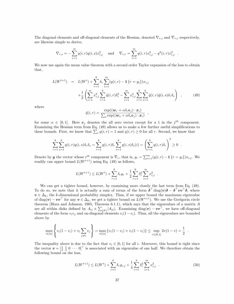
The diagonal elements and off-diagonal elements of the Hessian, denoted ∇r,s and ∇r,r respectively,are likewise simple to derive,

∇r,s = −m∑

i=1

q(i, r)q(i, s)x2i,j and ∇r,r =

m∑

i=1

q(i, r)x2i,j − q2(i, r)x2

i,j .

We now use again the mean value theorem with a second order Taylor expansion of the loss to obtainthat,

L(W t+1) = L(W t) +

k∑

r=1

δr

m∑

i=1

(q(i, r) − 1 r = yi)xi,j

+1

2

(m∑

i=1

x2i,j

k∑

r=1

q(i, r)δ2r −

m∑

i=1

x2i,j

k∑

r=1

k∑

s=1

q(i, r)q(i, s)δrδs

)

, (49)

where

q(i, r) =exp((wr + αδrej) · xi)

∑

s exp((ws + αδsej) · xi),

for some α ∈ [0, 1]. Here ej denotes the all zero vector except for a 1 in the jth component.Examining the Hessian term from Eq. (49) allows us to make a few further useful simplifications tothese bounds. First, we know that

∑

r q(i, r) = 1 and q(i, r) ≥ 0 for all r. Second, we know that

k∑

r=1

k∑

s=1

q(i, r)q(i, s)δrδs =

k∑

r=1

q(i, r)δr

k∑

s=1

q(i, s)δs(i) =

(k∑

r=1

q(i, r)δr

)2

≥ 0 .

Denote by g the vector whose rth component is ∇r, that is, gr =∑m

i=1(q(i, r)− 1 r = yi)xi,j . Wereadily can upper bound L(W t+1) using Eq. (49) as follows,

L(W t+1) ≤ L(W t) +

k∑

r=1

δrgr +1

2

k∑

r=1

δ2r

m∑

i=1

x2i,j .

We can get a tighter bound, however, by examining more closely the last term from Eq. (49).To do so, we note that it is actually a sum of terms of the form δ⊤ diag(v)δ − δ⊤vv⊤δ, wherev ∈ ∆k, the k-dimensional probability simplex. Thus, if we upper bound the maximum eigenvalueof diag(v) − vv⊤ for any v ∈ ∆k, we get a tighter bound on L(W t+1). We use the Gersgorin circletheorem (Horn and Johnson, 1985, Theorem 6.1.1), which says that the eigenvalues of a matrix Aare all within disks defined by Aii ±

∑

j 6=i |Aji|. Examining diag(v) − vv⊤, we have off-diagonalelements of the form vivj and on-diagonal elements vi(1−vi). Thus, all the eigenvalues are boundedabove by

maxi∈[n]

vi(1 − vi) + vi

∑

j 6=i

vj

= max

i∈[n]vi(1 − vi) + vi(1 − vi) ≤ sup

v∈[0,1]

2v(1 − v) =1

2.

The inequality above is due to the fact that vi ∈ [0, 1] for all i. Moreover, this bound is tight sincethe vector v = [12

12 0 · · · 0]⊤ is associated with an eigenvalue of one half. We therefore obtain the

following bound on the loss,

L(W t+1) ≤ L(W t) +

k∑

r=1

δrgr,j +1

4

k∑

r=1

δ2r

m∑

i=1

x2i,j . (50)

37

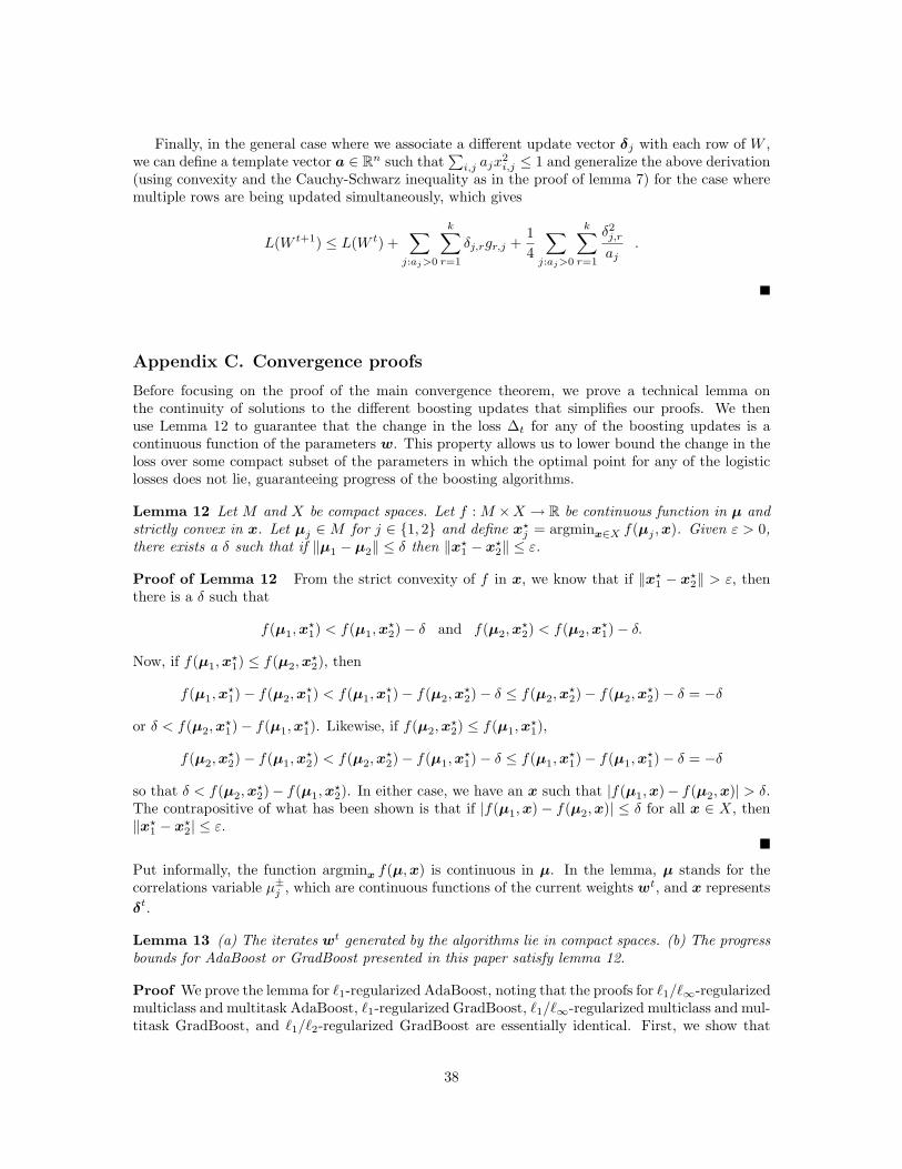
Finally, in the general case where we associate a different update vector δj with each row of W ,we can define a template vector a ∈ R

n such that∑

i,j ajx2i,j ≤ 1 and generalize the above derivation

(using convexity and the Cauchy-Schwarz inequality as in the proof of lemma 7) for the case wheremultiple rows are being updated simultaneously, which gives

L(W t+1) ≤ L(W t) +∑

j:aj>0

k∑

r=1

δj,rgr,j +1

4

∑

j:aj>0

k∑

r=1

δ2j,r

aj.

Appendix C. Convergence proofs

Before focusing on the proof of the main convergence theorem, we prove a technical lemma onthe continuity of solutions to the different boosting updates that simplifies our proofs. We thenuse Lemma 12 to guarantee that the change in the loss ∆t for any of the boosting updates is acontinuous function of the parameters w. This property allows us to lower bound the change in theloss over some compact subset of the parameters in which the optimal point for any of the logisticlosses does not lie, guaranteeing progress of the boosting algorithms.

Lemma 12 Let M and X be compact spaces. Let f : M ×X → R be continuous function in µ andstrictly convex in x. Let µj ∈ M for j ∈ 1, 2 and define x⋆

j = argminx∈X f(µj ,x). Given ε > 0,there exists a δ such that if ‖µ1 − µ2‖ ≤ δ then ‖x⋆

1 − x⋆2‖ ≤ ε.

Proof of Lemma 12 From the strict convexity of f in x, we know that if ‖x⋆1 − x⋆

2‖ > ε, thenthere is a δ such that

f(µ1,x⋆1) < f(µ1,x

⋆2) − δ and f(µ2,x

⋆2) < f(µ2,x

⋆1) − δ.

Now, if f(µ1,x⋆1) ≤ f(µ2,x

⋆2), then

f(µ1,x⋆1) − f(µ2,x

⋆1) < f(µ1,x

⋆1) − f(µ2,x

⋆2) − δ ≤ f(µ2,x

⋆2) − f(µ2,x

⋆2) − δ = −δ

or δ < f(µ2,x⋆1) − f(µ1,x

⋆1). Likewise, if f(µ2,x

⋆2) ≤ f(µ1,x

⋆1),

f(µ2,x⋆2) − f(µ1,x

⋆2) < f(µ2,x

⋆2) − f(µ1,x

⋆1) − δ ≤ f(µ1,x

⋆1) − f(µ1,x

⋆1) − δ = −δ

so that δ < f(µ2,x⋆2)− f(µ1,x

⋆2). In either case, we have an x such that |f(µ1,x)− f(µ2,x)| > δ.

The contrapositive of what has been shown is that if |f(µ1,x) − f(µ2,x)| ≤ δ for all x ∈ X, then‖x⋆

1 − x⋆2| ≤ ε.

Put informally, the function argminx f(µ,x) is continuous in µ. In the lemma, µ stands for thecorrelations variable µ±

j , which are continuous functions of the current weights wt, and x represents

δt.

Lemma 13 (a) The iterates wt generated by the algorithms lie in compact spaces. (b) The progressbounds for AdaBoost or GradBoost presented in this paper satisfy lemma 12.

Proof We prove the lemma for ℓ1-regularized AdaBoost, noting that the proofs for ℓ1/ℓ∞-regularizedmulticlass and multitask AdaBoost, ℓ1-regularized GradBoost, ℓ1/ℓ∞-regularized multiclass and mul-titask GradBoost, and ℓ1/ℓ2-regularized GradBoost are essentially identical. First, we show that

38

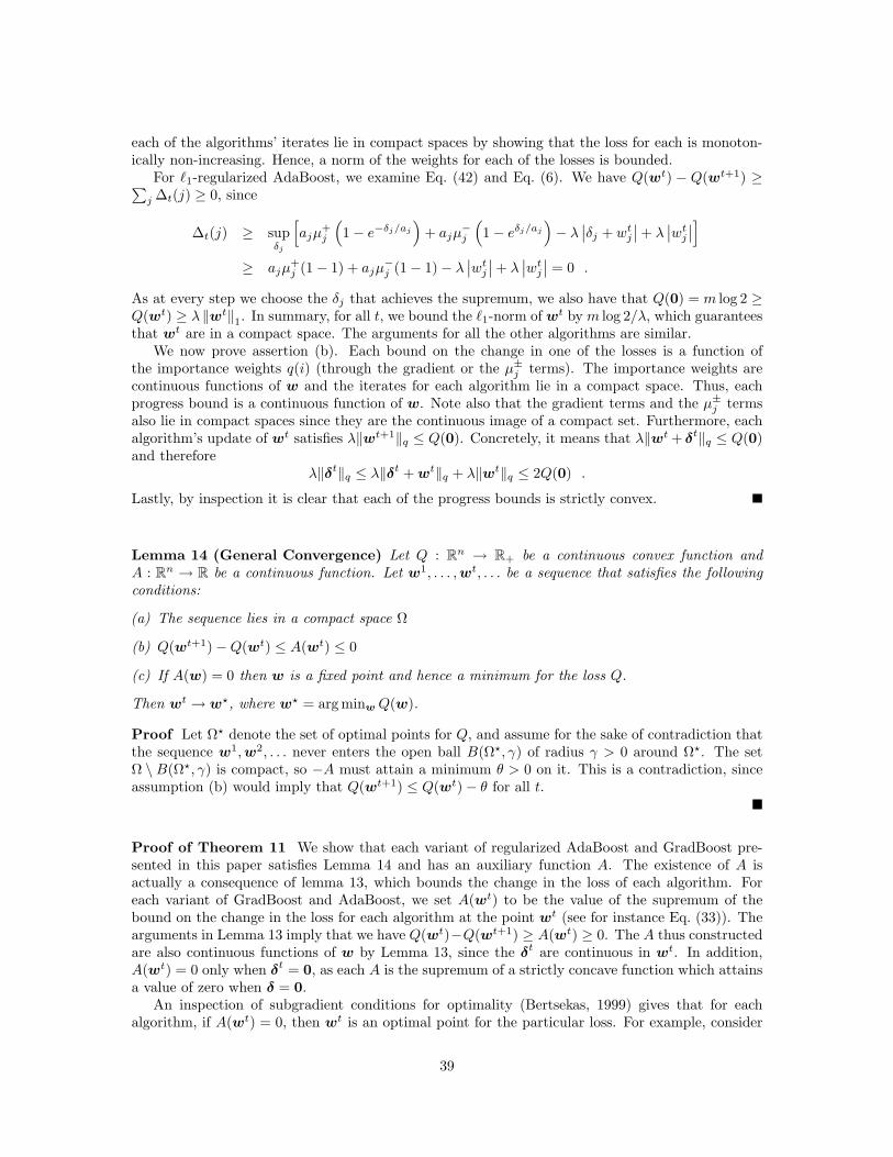
each of the algorithms’ iterates lie in compact spaces by showing that the loss for each is monoton-ically non-increasing. Hence, a norm of the weights for each of the losses is bounded.

For ℓ1-regularized AdaBoost, we examine Eq. (42) and Eq. (6). We have Q(wt) − Q(wt+1) ≥∑

j ∆t(j) ≥ 0, since

∆t(j) ≥ supδj

[

ajµ+j

(

1 − e−δj/aj

)

+ ajµ−j

(

1 − eδj/aj

)

− λ∣∣δj + wt

j

∣∣+ λ

∣∣wt

j

∣∣

]

≥ ajµ+j (1 − 1) + ajµ

−j (1 − 1) − λ

∣∣wt

j

∣∣+ λ

∣∣wt

j

∣∣ = 0 .

As at every step we choose the δj that achieves the supremum, we also have that Q(0) = m log 2 ≥Q(wt) ≥ λ ‖wt‖1. In summary, for all t, we bound the ℓ1-norm of wt by m log 2/λ, which guaranteesthat wt are in a compact space. The arguments for all the other algorithms are similar.

We now prove assertion (b). Each bound on the change in one of the losses is a function ofthe importance weights q(i) (through the gradient or the µ±

j terms). The importance weights arecontinuous functions of w and the iterates for each algorithm lie in a compact space. Thus, eachprogress bound is a continuous function of w. Note also that the gradient terms and the µ±

j termsalso lie in compact spaces since they are the continuous image of a compact set. Furthermore, eachalgorithm’s update of wt satisfies λ‖wt+1‖q ≤ Q(0). Concretely, it means that λ‖wt + δt‖q ≤ Q(0)and therefore

λ‖δt‖q ≤ λ‖δt + wt‖q + λ‖wt‖q ≤ 2Q(0) .

Lastly, by inspection it is clear that each of the progress bounds is strictly convex.

Lemma 14 (General Convergence) Let Q : Rn → R+ be a continuous convex function and

A : Rn → R be a continuous function. Let w1, . . . ,wt, . . . be a sequence that satisfies the following

conditions:

(a) The sequence lies in a compact space Ω

(b) Q(wt+1) − Q(wt) ≤ A(wt) ≤ 0

(c) If A(w) = 0 then w is a fixed point and hence a minimum for the loss Q.

Then wt → w⋆, where w⋆ = arg minw Q(w).

Proof Let Ω⋆ denote the set of optimal points for Q, and assume for the sake of contradiction thatthe sequence w1,w2, . . . never enters the open ball B(Ω⋆, γ) of radius γ > 0 around Ω⋆. The setΩ \ B(Ω⋆, γ) is compact, so −A must attain a minimum θ > 0 on it. This is a contradiction, sinceassumption (b) would imply that Q(wt+1) ≤ Q(wt) − θ for all t.

Proof of Theorem 11 We show that each variant of regularized AdaBoost and GradBoost pre-sented in this paper satisfies Lemma 14 and has an auxiliary function A. The existence of A isactually a consequence of lemma 13, which bounds the change in the loss of each algorithm. Foreach variant of GradBoost and AdaBoost, we set A(wt) to be the value of the supremum of thebound on the change in the loss for each algorithm at the point wt (see for instance Eq. (33)). Thearguments in Lemma 13 imply that we have Q(wt)−Q(wt+1) ≥ A(wt) ≥ 0. The A thus constructedare also continuous functions of w by Lemma 13, since the δt are continuous in wt. In addition,A(wt) = 0 only when δt = 0, as each A is the supremum of a strictly concave function which attainsa value of zero when δ = 0.

An inspection of subgradient conditions for optimality (Bertsekas, 1999) gives that for eachalgorithm, if A(wt) = 0, then wt is an optimal point for the particular loss. For example, consider

39

the ℓ1-regularized logistic loss of Eq. (2). Suppose that for every template a, no progress can bemade and δj = 0 for all j. Then, for all j we get that 0 belongs in the sub-differential set of thechange in the loss at δj = 0, namely,

0 ∈ −µ+j + µ−

j + λ∂δj|wj + δj |

∣∣δj=0

= −µ+j + µ−

j + λ∂|wj | .

Expanding the right hand side of the above equation, we get

−µ+j + µ−

j + λ∂|wj | = −∑

i:xi,jyi>0

q(i) |xi,j | +∑

i:xi,jyi<0

q(i) |xi,j | + λ∂|wj |

= −∑

i:xi,jyi>0

yixi,j

1 + eyi(w·xi)−

∑

i:xi,jyi<0

yixi,j

1 + eyi(w·xi)+ λ∂|wj |

= −m∑

i=1

1

1 + eyi(w·xi)yixi,j + λ∂|wj | =

∂

∂wjL(w) + ∂jλ ‖w‖1 ,

where ∂j is the subdifferential of Q(w) for the jth element of w. Thus, when the change in the lossis 0, we have that 0 is in the subdifferential of Q(w) for each wj and therefore w is an optimumof loss function. Lemma 13 guarantees that each algorithm’s iterates lie in a compact space, andtherefore Lemma 14 applies.

Appendix D. Experimental Setup

Feature Selection for ℓ2-Regularized Logistic Regression: Here we describe the featurescoring scheme to select the features used by ℓ2-regularized logistic regression. We first learnedthe base regressor (which can be done exactly), then we chose the 800 features that gave the bestdecrease in the loss. We show next that the latter stage reduces to selection based on an informationgain criterion. First, for selecting the bias weight b, we minimize

m∑

i=1

log(1 + exp(−yib)) = m+ log(1 + exp(−b)) + m− log(1 + exp(b))

where m+ and m− are the number of positive and negative examples, respectively. Taking thederivative and setting the result to zero, we get

−m+ 1

1 + eb+ m− eb

1 + eb= 0 ⇒ −m+ + m−eb = 0 ⇒ b = log

(m+

m−

)

. (51)

For the Reuters data, our features took values in 0, 1. Let us denote by n+j the number of examples

for which feature j was 1 and yi = 1 and by n−j the examples for which feature j was 1 while yi was

−1. Using these definitions, we want to minimize, w.r.t α, the following expression,

∑

i:xi,j 6=0

log(1 + exp(−yi(b + αxi,j))) = n+j log(1 + exp(−b − α)) + n−

j log(1 + exp(b + α)).

Again taking the derivative w.r.t α, we need solve − n+j

1+eb+α +n−

j

1+e−b−α = 0. Note that this expression

takes the same form as Eq. (51) for b. Thus, we obtain that b + α = log

(n+

j

n−

j

)

. To score a feature,

40

we simply compute the score ∆j , which is, ignoring the terms that only have to do with the bias b,

∆j = n+j log

(

1 +n−

j

n+j

)

+ n−j log

(

1 +n+

j

n−j

)

− n+j log

(

1 +m−

m+

)

− n−j log

(

1 +m+

m−

)

= −n+j log

(

n+j

n+j + n−

j

)

− n−j log

(

n−j

n+j + n−

j

)

+ n+j log

(m+

m+ + m−

)

+ n−j log

(m−

m+ + m−

)

= −DKL

(

n+j

n+j + n−

j

∥∥∥∥∥

m+

m+ + m−

)

(n+j + n−

j ) .

To recap, we choose the features with maximum KL-divergence from the base distribution of positiveand negative examples, weighted by the number of times the feature is on.

41