ieee transactions on image processing, …big · hessian schatten-norm regularization for linear...

IEEE TRANSACTIONS ON IMAGE PROCESSING, VOL. 22, NO. 5, MAY 2013 1873

Hessian Schatten-Norm Regularization forLinear Inverse Problems

Stamatios Lefkimmiatis, Member, IEEE, John Paul Ward, and Michael Unser, Fellow, IEEE

Abstract— We introduce a novel family of invariant, convex,and non-quadratic functionals that we employ to derive regular-ized solutions of ill-posed linear inverse imaging problems. Theproposed regularizers involve the Schatten norms of the Hessianmatrix, which are computed at every pixel of the image. Theycan be viewed as second-order extensions of the popular total-variation (TV) semi-norm since they satisfy the same invarianceproperties. Meanwhile, by taking advantage of second-orderderivatives, they avoid the staircase effect, a common artifactof TV-based reconstructions, and perform well for a widerange of applications. To solve the corresponding optimizationproblems, we propose an algorithm that is based on a primal-dual formulation. A fundamental ingredient of this algorithm isthe projection of matrices onto Schatten norm balls of arbitraryradius. This operation is performed efficiently based on a directlink we provide between vector projections onto �q norm ballsand matrix projections onto Schatten norm balls. Finally, wedemonstrate the effectiveness of the proposed methods throughexperimental results on several inverse imaging problems withreal and simulated data.

Index Terms— Eigenvalue optimization, Hessian operator,image reconstruction, matrix projections, Schatten norms.

I. INTRODUCTION

L INEAR inverse problems arise in a host of imaging appli-cations, ranging from microscopy and medical imaging

to remote sensing and astronomical imaging [1]. The task isto reconstruct the underlying image from a series of degradedmeasurements. These problems are often formulated within avariational framework, where image reconstruction can be castas the minimization of an energy functional subject to somepenalty. The role of the penalty is significant, since it imposescertain constraints on the solution and considerably affects thequality of the reconstruction.

The importance of choosing an appropriate penalty hasinitiated the development of regularization functionals thatcan effectively model certain properties of natural images.A popular regularization criterion is the total-variation (TV)semi-norm [2] which has been successfully applied to several

Manuscript received April 27, 2012; revised December 7, 2012; acceptedDecember 17, 2012. Date of publication January 4, 2013; date of currentversion March 14, 2013. This work was supported in part by the HaslerFoundation, the ERC Grant ERC-2010-AdG 267439-FUN-SP, and the Indo-Swiss Joint Research Program. The associate editor coordinating the reviewof this manuscript and approving it for publication was Dr. Alessandro Foi.

The authors are with the Biomedical Imaging Group, École Polytech-nique Fédérale de Lausanne, Lausanne CH-1015, Switzerland (e-mail:[email protected]; [email protected]; [email protected]).

Color versions of one or more of the figures in this paper are availableonline at http://ieeexplore.ieee.org.

Digital Object Identifier 10.1109/TIP.2013.2237919

imaging problems such as image denoising, restoration [3],[4], inpainting [5], zooming [6], and MRI reconstruction [7].TV owes its success to its ability to preserve the edges ofthe underlying image well. Its downside, however, is that itintroduces blocking artifacts (a.k.a. staircase effect) [8]. Thereason is that TV favors vanishing first-order derivatives. Thus,it tends to result in piecewise-constant solutions even whenthe underlying images are not necessarily piecewise constant.This tendency is responsible for oversharpening the contrastalong image contours and can be a serious drawback in manyapplications.

A common workaround to prevent the oversharpening ofregions with smooth intensity transitions is to replace TVby functionals that involve higher-order differential opera-tors, because higher-order derivatives can potentially restore awider class of images. Often, moving from piecewise-constantto piecewise-linear reconstructions offers a satisfactoryimprovement in the fitting of smooth intensity changes, sothat most of the published functionals involve second-orderdifferentials. Such regularizers have been considered, mostlyfor image denoising, either combined with TV [8]–[12] orin a standalone way [13]–[17]. These recent advances moti-vate us to investigate a class of regularizers that dependon matrix norms of the Hessian. These regularizers enjoymost of the favorable properties of TV; namely, convexity,contrast, rotation, translation, and scale invariance (up to amultiplicative constant), while they avoid the staircase effectby not penalizing first-order polynomials.

The key contributions of this work are as follows:1) The identification of a novel family of invariant function-

als that involve Schatten norms of the Hessian matrix,computed at every pixel of the image. These are usedin a variational framework to derive regularized solu-tions of ill-posed linear inverse imaging problems. Ourfunctionals capture curvature information related to theimage intensity and lead to reconstructions that avoidthe staircase effect.

2) A general first-order algorithm for solving the resultingconstrained optimization problems under any choice ofSchatten norm. The proposed algorithm relies on ourderivation of a primal-dual formulation and copes withthe non-smooth nature and the high dimensionality ofthe problem.

3) A direct link between matrix projections onto Schattennorm balls and vector projections onto �q norm balls.This link enables us to design an efficient method forperforming matrix projections. Although it is a funda-

1057-7149/$31.00 © 2013 IEEE

1874 IEEE TRANSACTIONS ON IMAGE PROCESSING, VOL. 22, NO. 5, MAY 2013

mental component of our optimization algorithm, ourresult is not specific to the Hessian and can potentiallyhave a wider applicability.

The rest of the paper is organized as follows: In Section II,we discuss regularization functionals that are commonly usedin imaging problems. Then, by focusing on invariance princi-ples we derive our novel family of non-quadratic second-orderfunctionals. In Section III, we present the discrete formulationof the problem and we describe the proposed optimizationalgorithm. In Section IV, we assess the performance of ourapproach for several linear inverse imaging problems withexperiments on standard test images and real biomedicalimages. We conclude our work in Section V. Proofs ofmathematical statements are given in Appendices.

II. DERIVATIVE-BASED REGULARIZATION

The most commonly-used regularizers can be expressed as

R ( f ) =∫�� (D f (r)) dr , (1)

where f is an image, � ⊂ R2, D is the regularization

operator (scalar or multi-component) acting on the image,and �(·) is a potential function. Typical choices for D aredifferential operators such as the Laplacian (scalar operator)or the gradient (vectorial operator), while the potential function� usually involves a norm distance. For many years, thepreferred choice for the potential function has been the squaredEuclidean norm, because of its mathematical tractability andcomputational simplicity. However, it is now widely doc-umented that non-quadratic potential functions can lead toimproved results; they can be designed to be less sensitiveto outliers and therefore provide better edge reconstruction. Atypical example is TV, which for smooth images correspondsto the L1 norm of the magnitude of the gradient.

Our present goal is to introduce new regularization func-tionals of the form of (1) which amounts to specifying somesuitable linear operator D, and potential function �. To doso, certain requirements should be fulfilled. In particular,following the example of TV, we restrict ourselves to regular-ization operators that commute with translation and scaling,and potential functions that preserve these properties whileintroducing additional rotation invariance. Our motivation forenforcing these invariances is that, similarly to what is thecase in many physical systems, one should opt for reconstruc-tion algorithms that lead to solutions which are not affectedby transformations of the coordinate system. An additionaldesirable requirement is that the regularizers should be convexto ensure that if a minimum exists, then this is a globalone. Furthermore, convexity permits the design of efficientminimization techniques.

A. Gradient Norm Regularization

We would like our regularization operator to be translationand scale invariant. Therefore, a reasonable choice for D issome form of derivative operator. Based on this, we firstcharacterize the complete class of gradient-based regularizerssatisfying all the required invariances. This is accomplished

by Theorem 1 which specifies the valid form for the potentialfunctions�. The proof of this theorem is given in Appendix I.

Theorem 1: Let R ( f ) be of the form (1), where D is thegradient operator and f is continuously differentiable. R ( f ) isa translation-, rotation-, and scale-invariant functional, if andonly if the potential function � : R

2 �→ R is of the form:�(∇ f (r)) = c |∇ f (r)|ν , where ν ∈ R and c is an arbitraryconstant.

As a direct consequence of Theorem 1, we see that thefollowing gradient-based regularizers are the only choice ofregularization satisfying the required invariance properties;ignoring the multiplicative constant c of the potential function,which can be absorbed by the regularization parameter, we get

R ( f ) =∫�

|∇ f (r)|ν dr . (2)

Since we are also interested in convex regularization function-als, we shall focus on cases where ν ≥ 1 in (2). A popularinstance of convex functionals arises if we choose ν = 1,which corresponds to TV. This regularizer enjoys an additionalproperty, that of contrast covariance.

B. Hessian Schatten-Norm Regularization

As already mentioned, the use of TV, which is the bestrepresentative of the gradient-based regularization family, suf-fers from certain drawbacks. Therefore, for the reasons speci-fied in the introduction, we are interested in differential oper-ators of higher-order and in particular of the second order. InN-dimensions, the complete spectrum of second-order deriv-atives is embodied in the Hessian operator,

H f (r) =[

fr1r1 (r) fr1r2 (r)fr2r1 (r) fr2r2 (r)

], (3)

where fri r j (r) = ∂2

∂ri ∂r jf (r). Indeed, with the aid of the

Hessian we can compute any second-order derivative of f (r)as D2

θ,φ f (r) = uTθ H f (r) vφ , where uθ = (cos θ, sin θ)

and vφ = (cosφ, sin φ) are unit-norm vectors specifying thedirections of differentiation and (·)T is the transpose operation.

Having specified the regularization operator D, the nextstep is to investigate which class of potential functions �leads to translation-, rotation-, and scale-invariant second-orderregularizers. Next, we provide Theorem 2 which completelycharacterizes the form of �, under these prerequisites. Beforepresenting this result, we first give the general definition of aSchatten matrix norm [18] that will be used in the sequel, andintroduce some of the adopted notation. We denote the set ofunitary matrices as U

n = {X ∈ C

n×n : X−1 = XH}, where C

is the set of complex numbers and (·)H is the Hermitian trans-pose. We also denote the set of positive semidefinite diagonalmatrices as D

n1×n2 ={

X ∈ Rn1×n2+ : X (i, j) = 0 ∀ i = j

},

where R+ is the set of real non-negative numbers.Definition 1 (Schatten Norms): Let X ∈ C

n1×n2 bea matrix with the singular-value decomposition (SVD)X = U�VH , where U ∈ U

n1 and V ∈ Un2 consist of the

singular vectors of X, and � ∈ Dn1×n2 consists of the singular

values of X. The Schatten norm of order p (Sp norm) of X is

LEFKIMMIATIS et al.: HESSIAN SCHATTEN-NORM REGULARIZATION 1875

defined as

‖X‖Sp =⎛⎝min(n1,n2)∑

k=1

σp

k (X)

⎞⎠

1p

, (4)

where p ≥ 1, and σk (X) is the k-th singular value of X, whichcorresponds to the (k, k) entry of �.

Definition 1 implies that the Sp norm of a matrix Xcorresponds to the �p norm of its singular-values vectorσ (X) ∈ R

min(n1,n2)+ . This further means that all Schatten normsare unitarily invariant. Moreover, we note that the family of Sp

norms includes three of the most popular matrix norms, i.e.,the nuclear/trace norm (p = 1), the Frobenius norm (p = 2)and the spectral/operator norm (p = ∞).

Theorem 2: Let R ( f ) be of the form (1), where D is theHessian operator and f is twice continuously differentiable.R ( f ) is a translation-, rotation-, and scale-invariant functional,if and only if the potential function � : R

2×2 �→ R is of theform: �(H f (r)) = �0

(λ f (r) / ‖H f (r)‖Sp

)‖H f (r)‖νSp

,where ν ∈ R and �0 is a zero-degree homogeneous functionof the Hessian eigenvalues λ f (r).

The proof of Theorem 2 is given in Appendix I. Now,according to it, the admissible second-order regularizers, withrespect to the invariance properties of the coordinate system,are those depending on the Schatten norms of the Hessian. Ifwe set �0 = 1, we obtain the following regularization family

R ( f ) =∫�

‖H f (r)‖νSpdr ,∀p ≥ 1 and ν ∈ R . (5)

To further ensure convexity we need to impose thatν ≥ 1. Finally, for our regularizers to also enjoy the contrast-covariance property (similar to TV), we focus on the casewhere ν = 1. Consequently, we define our proposed family ofnon-quadratic second-order regularization functionals as

R ( f ) =∫�

‖H f (r)‖Spdr ,∀p ≥ 1 . (6)

The introduced functionals, depending on the Hessian, leadto piecewise-linear reconstructions. These reconstructions canbetter approximate the intensity variations observed in naturalimages than the piecewise-constant reconstructions providedby TV. Thus, they are able to avoid the staircase effect.Moreover, since the Hessian of f at coordinates r is a 2 × 2symmetric matrix, the SVD in the Schatten norm definitionreduces to the spectral decomposition and the singular valuescorrespond to the absolute eigenvalues, which can be com-puted analytically. Now, if we consider the intensity map of theimage as a 3-D differentiable surface, then the two eigenvaluesof the Hessian at coordinates r correspond to the principalcurvatures. They can be used to measure how this surfacebends by different amounts in different directions at that point.Therefore, the proposed potential functions, which dependupon those, can be interpreted as scalar measurements of thecurvature at a local surface patch. For example, the S2 norm(Frobenius norm) of the Hessian is a scalar curvature index,commonly used in differential geometry, which quantifies lackof flatness of the surface at a specific point. Therefore, we

can safely state that the proposed regularizers incorporatecurvature information about the image intensity.

Finally, we note that the regularizers obtained for twochoices of p = 2,∞, coincide with functionals we consideredin our previous work in [19], where we followed another pathfor extending TV based on rotational averages of directionalderivatives. To the best of our knowledge, the Hessian Schattennorms for p = 2,∞ have not been considered before in thecontext of inverse problems.

III. VARIATIONAL IMAGE RECONSTRUCTION

From now on, we focus on the discrete formulation of imagereconstruction. Hereafter, to avoid any confusion between thecontinuous and the discrete domains we will use bold-facedsymbols to refer to the discrete manipulation of the problem.

A. Discrete Problem Formulation

Our approach for reconstructing the underlying image fromthe measurements is based on the linear observation model

y = Ax + w , (7)

where A ∈ RM×N is a matrix that models the spatial response

of the imaging device, while y ∈ RM and x ∈ R

N are thevectorized versions of the observed image and the image tobe estimated, respectively. Apart from the effect of the operatorA acting on the underlying image, another perturbation is themeasurement noise, which is intrinsic in the detection process.This degradation factor is represented in our observation modelby w that we, here on, will assume to be i.i.d Gaussian noisewith variance σ 2

w.The recovery of x from the measurements y belongs to the

category of linear inverse problems. Usually, for the cases ofpractical interest, it is ill-posed [20]: the operator A is eitherill-conditioned or singular. This is dealt with in the variationalframework by forming an objective function

ϕ (x) = 1

2‖y − Ax‖2

2 + τψ (x) , (8)

whose role is to quantify the quality of a given estimate.The first term, also known as data fidelity, corresponds tothe negative Gaussian log-likelihood and measures how wella candidate estimate explains the observed data. The secondterm (regularization) encodes our beliefs about certain char-acteristics of the underlying image. Its role is to narrow downthe set of plausible solutions by penalizing those that do notsatisfy the assumed properties. The parameter τ ≥ 0 provides abalance between the contribution of the two terms. The imagereconstruction problem is then cast as the minimization of (8)and leads to a penalized least-squares solution.

B. Discrete Hessian Operator and Basic Notations

In this work we focus on the class of Hessian Schatten-normregularizers presented in (6). In the sequel, we use H to referto the discrete version of the Hessian operator. To simplify ouranalysis, we assume that the image intensities on a Nx × Ny

grid are rasterized in a vector x of size N = Nx · Ny , so thatthe pixel at coordinates (i , j) maps to the nth entry of x withn = j Nx +(i +1). In this case, the discrete Hessian operator is


a mapping H : RN �→ X , where X = R

N×2×2. For x ∈ RN ,

Hx is given as

[Hx]n =[ [ r1r1 x

]n

[ r1r2 x

]n[

r1r2 x]

n

[ r2r2 x

]n

], (9)

where [·]n denotes the nth element of the argument, n =1 , . . . , N , and r1r1 , r2r2 , and r1r2 denote the forwardfinite-difference operators [21] that approximate the second-order partial derivatives along the two dimensions of theimage. If we assume Neumann boundary conditions anduse the standard representation of the image rather than thevectorized one, these operators are defined as

[ r1r1 x

]i, j =

{xi+2, j −2xi+1, j + xi, j , 1≤ i ≤ Nx − 2,

xNx −1, j − xNx , j , i ≥ Nx − 1,(10a)

[ r2r2 x

]i, j =

{xi, j+2−2xi, j+1 + xi, j , 1≤ j ≤ Ny − 2,

xi,Ny −1 − xi,Ny , j ≥ Ny − 1,(10b)

[ r1r2 x

]i, j =

⎧⎪⎨⎪⎩

xi+1, j+1 − xi+1, j − xi, j+1 + xi, j ,

1 ≤ i ≤ Nx − 1 and 1 ≤ j ≤ Ny − 1,

0, otherwise .(10c)

We equip the space X with the inner product 〈· , ·〉X andnorm ‖·‖X . To define them, let X,Y ∈ X , with Xn,Yn ∈R

2×2 ∀ n = 1, . . . , N . Then we have

〈X , Y〉X =N∑

n=1

tr(

YTn Xn

)(11)

and

‖X‖X = √〈X , X〉X , (12)

where tr (·) is the trace operator. For the Euclidean space RN

we use the standard definition of the inner product and of thenorm. We denote them by 〈· , ·〉2 and ‖·‖2, respectively.

The adjoint of H is the discrete operator H∗ : X �→ RN

such that

〈Y , Hx〉X = ⟨H∗Y , x

⟩2 . (13)

This definition of the adjoint operator is a generalization ofthe Hermitian transpose for matrices. Based on the relation ofthe inner products in (13), we show in Appendix II that forany Y ∈ X , it holds that[

H∗Y]

n = [ ∗

r1r1Y(1,1)

]n

+ [ ∗

r2r2Y(2,2)

]n

+ [ ∗

r1r2

(Y(1,2) + Y(2,1)

)]n, (14)

where Y(i, j )n is the (i, j) entry of the 2 × 2 matrix Yn and

∗r1r1

, ∗r1r2

, ∗r2r2

are the adjoint operators that correspondto backward difference operators with Neumann boundaryconditions.

C. Majorization-Minimization Algorithm

Next, we present a general method to compute the mini-mizer of the functional in (8), under any Hessian-based Sp

norm regularizer. Since these regularizers are non-smooth,our algorithm is based on a majorization-minimization (MM)

approach (cf. [22], [23], [24] for instance). Under this frame-work, instead of directly minimizing (8), we find the solutionvia the successive minimization of a sequence of surrogatefunctions that upper bound the initial objective function [25].Our motivation for taking this path is that each of the surrogatefunctions is simpler to minimize, and we can rely on a gradientscheme that efficiently copes with the large dimensionality ofthe problem.

To obtain the surrogate functions, we upper bound thedata term of our objective function using the followingmajorizer [22], [26]

g (x, x0) = 1

2‖y − Ax‖2

2 + d (x, x0) , (15)

where d (x, x0) = 12 (x − x0)

T [αI − AT A

](x − x0) is a

function that measures the distance between x and x0. Tocome up with a valid majorizer we need to ensure thatd (x, x0) ≥ 0, ∀x, with equality if and only if x = x0. Thisprerequisite is true if αI − AT A is positive definite, whichimplies that α >

∥∥AT A∥∥. The upper-bounded version of the

overall objective (8) can be written as

ϕ (x, x0) = α

2‖x − z‖2

2 + τψ (x)+ c , (16)

where c is a constant and z = x0 + α−1AT (y − Ax0). Then,the next step is to iteratively minimize (16) w.r.t x, setting x0to the previous iteration’s solution. As we see, in (16) thereis no coupling between x and the operator A anymore, whichturns the minimization task into a much simpler one. In fact,the minimizer of (16) can also be interpreted as the solutionof a denoising problem with z being the noisy measurements.

D. Proximal Map Evaluation and Matrix Projections

The MM formulation of our problem relies on the solutionof a simpler problem of the form

x = arg minx∈Rn

1

2‖x − z‖2

2 + τψ (x)+ ιC (x) , (17)

where ιC is the indicator function of a convex set C that repre-sents additional constraints on the solution, such as positivityor box constraints. The convention is that ιC (x) takes the value0 for x ∈ C and ∞ otherwise. If ϑ (x) = τψ (x) + ιC (x) isa proper, closed, convex function, then the solution of (17) isunique and corresponds to the value of the Moreau proximityoperator [27], defined as

proxϑ (z) = arg minx∈RN

1

2‖x − z‖2

2 + ϑ (x) . (18)

The proximal map of ϑ (x) cannot always be obtained inclosed-form, and this is also the case for the regularizersunder study. For this reason, we next present a primal-dualapproach that results in a novel numerical algorithm, whichcan efficiently compute the solution.

A fundamental ingredient of our proposed algorithm is theorthogonal projection of matrices onto Sq norm balls. Thisprojection can be performed efficiently based on the followingproposition, which provides a direct link between vectorprojections onto �q norm balls and matrix projections onto Sq


norm balls. This result is new, to the best of our knowledge,and its proof is provided in Appendix II. A relevant result thatcan be considered as a converse statement of Proposition 1 canbe found in [28, Theorem A.2].

Proposition 1 (Schatten Norm Projections): Let Y∈Cn1×n2

with SVD decomposition Y = U�VH , where U ∈ Un1 ,

V ∈ Un2 and � ∈ D

n1×n2 . The orthogonal projection of Yonto the set BSq =

{X ∈ C

n1×n2 : ‖X‖Sq ≤ ρ}

is given by

PBSq(Y) = Udiag

(PBq (σ (Y))

)VH ,

where diag (·) is the operator that maps a vector to a diagonalmatrix and PBq is the orthogonal projection onto the �q norm

ball Bq ={

v ∈ Rmin(n1,n2)+ : ‖v‖q ≤ ρ

}of radius ρ.

Based on Proposition 1, we design an algorithm for theorthogonal projection of a matrix Y onto the convex set BSq .Our algorithm consists of three steps: (a) decompose Y in itssingular vectors and singular values by means of the SVD;(b) project its singular values onto the corresponding �q normball Bq ; and (c) obtain the projected matrix via singular valuereconstruction (SVR) using the projected singular values andthe original singular vectors.

We next describe all of the steps leading to the proposedalgorithm that solves the problem

arg minx∈C

1

2‖x − z‖2

2 + τ ‖Hx‖1,p ∀p ≥ 1 . (19)

With ‖Hx‖1,p we denote the discrete version of ourproposed regularization family (6), where ‖·‖1,p standsfor the mixed �1-Sp norm, which for an argument � =[�T

1 ,�T2 , . . . ,�

TN

]T ∈ X is defined as

‖�‖1,p =N∑

n=1

‖�n‖Sp ,∀p ≥ 1 . (20)

The discrete form of our regularizers highlights their relationto the sparsity-promoting group norms, which are commonlymet in the context of compressive sensing (see [29], forinstance). However, a significant difference is that in our casethe mixed norm is a vector-matrix norm rather than a vector-vector norm. Therefore, while the machinery we are usingshares some similarities with the one employed in the groupvector-norm case, there are important differences, with themost pronounced being the projection step.

Since the operator of our choice is the Hessian, whichproduces 2 × 2 symmetric matrices at every coordinate ofx, �n ∈ S

2 in (20), where S2 = {

X ∈ R2×2 : XT = X

}.

However, for reasons of completeness, in the following lemma,where we derive the dual of the �1-Sp norm, we consider themore general case �n ∈ C

n1×n2 . The proof of Lemma 1 isprovided in Appendix II and follows a similar line of thoughtwith the one presented in [30, Lemma 1]. The latter is aboutthe dual norm of a mixed �1-�p vector norm.

Lemma 1: Let p ≥ 1, and let q be the conjugate exponentof p, i.e., 1

p + 1q = 1. Then, the mixed norm ‖·‖∞,q is dual

to the mixed norm ‖·‖1,p.

Using Lemma 1 and noting that the dual of the dual norm isthe original norm [31], we write (20) in the equivalent form

‖�‖1,p = max�∈B∞,q

〈� , �〉X , (21)

where B∞,q denotes the �∞-Sq unit-norm ball, defined as

B∞,q ={� =

[�T

1 ,�T2 , . . . ,�

TN

]T ∈ X :‖�n‖Sq ≤ 1,∀n = 1, . . . , N

}. (22)

This alternative definition of the mixed �1-Sp norm allow usto express it in terms of an inner product that involves the dualvariable � and the unit-norm ball B∞,q . Moreover, from (22)it is straightforward to see that the orthogonal projection ontoB∞,q is obtained by projecting separately each submatrix �n

onto a unit-norm Sq ball (BSq ).Using (21) we re-write (19) as

x = arg minx∈C

1

2‖x − z‖2

2 + τ max�∈B∞,q

〈� , Hx〉X . (23)

This formulation naturally leads us to the following minimaxproblem

minx∈C

max�∈B∞,q

L (x,�) , (24)

whereL (x,�) = 1

2‖x − z‖2

2 + τ⟨H∗� , x

⟩2 . (25)

Since the function L (x,�) is strictly convex in x and concavein �, we have the guarantee that a saddle-value is attained[31], and, thus, the order of the minimum and the maximumin (24) does not affect the solution. This means that there existsa saddle-point

(x, �

)that leads to a common value when the

minimum and the maximum are interchanged, i.e.,

minx∈C

max�∈B∞,q

L (x,�) = L(

x, �)

= max�∈B∞,q

minx∈C

L (x,�) .

(26)

Based on this observation, we can now define the primal anddual problems by identifying the primal and dual objectivefunctions, respectively. The l.h.s of (26) corresponds to theminimization of the primal objective function � (x), and ther.h.s to the maximization of the dual objective function s (�),

� (x) = max�∈B∞,q

L (x,�) = 1

2‖x − z‖2

2 + τ ‖Hx‖1,p ,(27)

s (�) = minx∈C

L (x,�)

= 1

2‖PC (v)− v‖2

2 + 1

2‖z‖2

2 − 1

2‖v‖2

2 , (28)

where PC is the orthogonal projection onto the convex setC and v = z − τH∗�. Therefore, (26) indicates that we canobtain the minimizer x of � (x) from the maximizer � of s (�)through the relation

x = PC

(z − τH∗�

). (29)

This last relation is important, since in contrast to the primalproblem (19), which is not continuously differentiable, thedual one involves the smooth function s (�). We can therefore


solve it by exploiting its gradient. Indeed, using the propertythat the gradient of a function h (x) = ‖x − PC (x)‖2

2 is welldefined and is equal to ∇h (x) = 2 (x − PC (x)) [4, Lemma4.1], we compute the gradient of s (�) as

∇s (�) = τH PC(z − τH∗�

). (30)

Therefore, the solution of our primal problem (19) is obtainedin two steps: (a) we find the maximizer of the dual objectivefunction (28) as described next, and (b) we obtain the solutionthrough (29).

E. Maximization of the Dual Objective

At this point, a main issue we need to deal with, is thatthe Hessian operator H does not have an empty null spaceand, thus, a stable inverse does not exist. Consequently, wecannot opt for a closed-form solution for the maximizer �of s (�). This means that we have to resort to a numericaliterative scheme. In this work, we employ Nesterov’s iterativemethod [32] for smooth functions. This is a gradient-basedscheme that exhibits convergence rates of one order higherthan the standard gradient-ascent method. To ensure conver-gence of the algorithm, we need to choose an appropriatestep-size. Since our dual objective is smooth with Lipschitzcontinuous gradient, we can use a constant step-size, thus,avoid a line search at every iteration. An appropriate step-sizeis equal to the inverse of the Lipschitz constant of ∇s (�).We derive an upper bound of this Lipschitz constant in thefollowing proposition, whose proof is given in Appendix II.

Proposition 2: Let L (s) denote the Lipschitz constant of∇s (�) of the dual objective function defined in (28). Then,it holds that

L (s) ≤ 64τ 2 . (31)

From (26) and (28) it is clear that the maximizer of ourdual objective can be derived by solving the constrainedmaximization problem

� = arg max�∈B∞,q

1

2‖PC (v)− v‖2

2 − 1

2‖v‖2

2 , (32)

with v = z − τH∗�. A necessary step towards this directionis to compute the projection onto the set B∞,q , defined in(22). This operation is accomplished by projecting indepen-dently each of the N components �n of � onto the setBSq =

{X ∈ S

2 : ‖X‖Sq ≤ 1}

. This projection is performedefficiently following the three steps of the algorithm weproposed in Section III-D, which is based on our Proposition 1.

Steps (a) and (c) are fairly easy to implement. Specifically,since the matrices of interest are 2×2 symmetric, we computethe SVD and the SVR steps in closed-form. Then, the mostcumbersome part of our algorithm is the �q norm projectionof the singular values, which for general values of q doesnot exist in closed form. Fortunately, this operation is stillfeasible thanks to the recently developed �q norm projectionalgorithm [30]. This projection method is based on an effi-cient proximity algorithm for �q norms [33]. Moreover, inSection III-F we report three cases of Sq norms, q = 1, 2,∞,whose projection can be evaluated in closed-form.

F. Closed Form of Sq -Norm Projections for q = 1, 2,∞.

From Proposition 1, we know that the matrix projection ontothe BS2 unit-norm ball is associated with the projection of thesingular values of the matrix onto the B2 ball. The latter iscomputed by normalizing the elements of the correspondingvector by their Euclidean norm. Therefore, we have that

PBS2(�n) =

{�n‖�n‖F

, if ‖�n‖F > 1

�n , if ‖�n‖F ≤ 1 .(33)

This situation is advantageous since it allows us to avoid boththe SVD and the SVR steps. Consequently, this drasticallyreduces the complexity of computing the projection. To com-pute the projection onto BS∞, we use that the projection ontothe B∞ unit-norm ball corresponds to setting the elements thathave an absolute value greater than one to one, and addingback their original sign. Therefore, we readily get

PBS∞ (�n) = Udiag (min (σ (�n) , 1))VH , (34)

where 1 is a vector with all elements set to one and themin operator is applied component-wise. Note that, this resultis directly related to the singular value thresholding (SVT)method [34], [35] developed in the field of matrix rankminimization. The derivation of SVT in [34], [35] is technical.It relies on the characterization of the subgradient of thenuclear norm [36]. By contrast, in our case the result comes outnaturally as an immediate consequence of Proposition 1 andof the duality between the spectral and nuclear matrix norms.Finally, the projection of a matrix onto the BS1 unit-norm ballis related to the projection of its singular values onto the B1unit-norm ball. The latter is computed by the soft-thresholdingoperator Sγ (σ (�n)) = max (σ (�n)− γ, 0) [37], where themax operator is applied component-wise. Therefore, based onProposition 1, we have that

PBS1(�n) = Udiag

(Sγ (σ (�n))

)VH . (35)

This last projection cannot in general be computed in closedform. The reason is that the threshold γ is not known inadvance and needs to be estimated. This can be accomplisedusing one of the existing methods available in the litera-ture [38]–[41]. Fortunately, in our case, the singular vectorsare of low dimensionality, σ (�n) ∈ R

2+ and, thus, we deriveγ analytically, as

γ =

⎧⎪⎪⎪⎨⎪⎪⎪⎩

0 , if σ1 (�n) ≤ 1 − σ2 (�n) ,

σ1(�n )+σ2(�n )−12 ,

if 1 − σ2 (�n) < σ1 (�n)

≤ 1 + σ2 (�n),

σ1 (�n)− 1 , if σ1 (�n) > 1 + σ2 (�n) ,

(36)

where the singular values are sorted in a decreasing order, i.e.,σ1 (�n) ≥ σ2 (�n).

G. Numerical Algorithm

Equipped with all the necessary ingredients, we concludewith a summarized description of the complete optimizationalgorithm. Our method consists of two components that inter-act. The first component is responsible for the majorizationof the objective function, as we described in Sec. III-C,


Algorithm 1 Image Reconstruction Algorithm Under Hessian-Based �1 − Sp Norm Regularization

while the second one undertakes the minimization of theresulting upper-bounded version. Then, the algorithm proceedsby iteratively minimizing the majorizer that is formed based onthe solution of the previous iteration. Since the convergenceof this scheme can be slow in practice, to speed it up weemploy the FISTA algorithm [24]. This method exhibits state-of-the-art convergence rates by combining two consecutiveiterates, in an optimum way. A description of our imagereconstruction approach that is based on the monotone versionof FISTA (MFISTA) [4] is given in Algorithm 1. The sub-routine denoise corresponds to the second component thatfinds the solution of (19). This minimizer is related to theproximal map proxτ

∥∥H ·∥∥1,pbut we can also interpret it as a

denoising step under Hessian-based �1-Sp norm regularization.The computation of the denoise sub-routine is described inAlgorithm 2 and is based on the primal-dual formulation thatwe proposed in Secs. III-D and III-E.

Finally, regarding the computational complexity of thealgorithm, it is only mildly higher than that of TV’s. Theextra computational cost is due to (a) the use of a tensor(Hessian) instead of a vectorial (gradient) operator and (b)the projections onto the BSq balls instead of the B2 ball. Ourprojections are somewhat more expensive because of the SVDand SVR steps. However, these steps are computed in closedform. It is also worth mentioning that the proposed algorithmis highly parallelizable, since all the involved operations are

Algorithm 2 Denoise (z, τ, p, Pc)—Denoising AlgorithmUnder Hessian-Based �1 − Sp Norm Regularization

performed independently for each pixel of the image.

IV. EXPERIMENTAL RESULTS

To evaluate the effectiveness of our proposed regularizationframework, we report results for several linear inverse imagingproblems. In particular, we consider the problems of imagedeblurring, sparse reconstruction from random samples, imageinterpolation and image zooming. For the image deblurringproblem we compare our results against those obtained byusing three alternative methods; namely, TV regularization,regularization with the fully redundant Haar wavelet transform,and the image deblurring version of the BM3D patch-basedmethod [42]. In Haar’s case, we use the frame analysis frame-work since it has been reported in the literature (c.f [43]) thatthe frame synthesis framework usually leads to inferior results.For the rest of the inverse problems we provide comparisonsagainst TV and quadratic derivative-based regularizers.

A. Restoration Setting

For the image deblurring experiments, we use a set of 8grayscale images1 which have been normalized so that theirintensities lie in the range of [0 , 1].

The performance of the methods under comparison isassessed for various blurring kernels and different noise levels.In particular, in our experiments we employ three point spreadfunctions (PSFs) to produce blurred versions of the images. Weuse a Gaussian PSF of standard deviation σb = 4, a movingaverage (uniform) PSF, and a motion-blur kernel. The first twoPSFs have a support of 9 × 9 pixel while the third one has asupport of 19 × 19 pixel. As an additional degradation factorwe consider Gaussian noise of three noise levels correspondingto a blurred signal-to-noise-ratio (BSNR) of {15, 20, 25} dB,respectively. The BSNR is defined as BSNR = var (Ax) /σ 2

w

1Three of these images along with the motion-blur kernel usedin the experiments were obtained from http://www.wisdom.weizmann.ac.il/~levina/papers/LevinEtalCVPR09Data.rar.


TABLE I

ISNR COMPARISONS OF IMAGE RESTORATION FOR THREE BLURRING KERNELS AND THREE NOISE LEVELS

Image Boat Face Fluor. Cells Hill House Kids Lena Peppers

BSNR 15 dB 20 dB 25 dB 15 dB 20 dB 25 dB 15 dB 20 dB 25 dB 15 dB 20 dB 25 dB 15 dB 20 dB 25 dB 15 dB 20 dB 25 dB 15 dB 20 dB 25 dB 15 dB 20 dB 25 dB

Gau

ssia

nB

lur Haar 2.34 2.77 3.71 2.37 2.80 3.88 2.36 2.41 3.19 2.61 2.48 2.95 2.56 3.23 4.27 3.20 3.50 4.45 2.84 2.67 3.20 2.30 3.43 5.10

TV 2.59 2.95 3.81 3.60 3.96 4.78 2.84 2.84 3.48 2.85 2.65 3.07 2.91 3.49 4.45 4.15 4.25 4.93 3.52 3.25 3.64 3.24 4.31 5.69H S∞ 2.63 3.03 3.88 4.32 4.71 5.62 3.61 3.62 4.32 2.95 2.74 3.22 3.28 3.92 4.92 4.33 4.61 5.42 3.60 3.42 3.91 3.52 4.35 5.59H S2 2.71 3.12 4.00 4.43 4.84 5.80 3.66 3.69 4.40 2.99 2.80 3.29 3.33 3.99 5.00 4.41 4.70 5.51 3.67 3.51 4.01 3.63 4.52 5.78H S1 2.75 3.18 4.07 4.45 4.88 5.84 3.65 3.70 4.41 3.00 2.82 3.32 3.33 3.97 4.99 4.42 4.70 5.53 3.71 3.55 4.06 3.71 4.67 5.93BM3D 2.88 3.37 4.32 4.75 5.14 6.08 3.70 3.75 4.39 3.04 3.00 3.51 3.51 4.07 4.92 4.51 4.66 5.27 3.78 3.70 4.24 3.79 4.76 5.91

Uni

form

Blu

r Haar 3.04 3.69 4.73 2.84 3.55 4.76 2.90 3.22 4.14 3.13 3.19 3.89 3.35 4.23 5.49 3.85 4.40 5.51 3.21 3.32 4.03 3.47 4.89 6.37TV 3.20 3.80 4.77 3.71 4.30 5.41 3.26 3.50 4.30 3.27 3.30 3.93 3.57 4.35 5.50 4.48 4.95 5.87 3.79 3.78 4.36 4.32 5.84 7.26H S∞ 3.22 3.84 4.81 4.38 4.95 6.16 3.92 4.20 5.04 3.32 3.39 4.06 3.87 4.78 6.00 4.62 5.13 6.15 3.85 3.89 4.52 4.39 5.75 7.03H S2 3.32 3.95 4.96 4.48 5.08 6.35 3.98 4.27 5.12 3.38 3.46 4.15 3.94 4.87 6.10 4.74 5.25 6.27 3.95 4.00 4.62 4.55 5.91 7.20H S1 3.36 4.02 5.05 4.51 5.13 6.41 3.99 4.28 5.13 3.40 3.50 4.18 3.95 4.88 6.09 4.77 5.29 6.30 4.00 4.04 4.68 4.66 6.03 7.32BM3D 3.48 4.19 5.26 4.97 5.80 6.81 3.97 4.29 5.06 3.53 3.68 4.35 4.05 4.91 5.97 4.70 5.03 5.91 4.06 4.18 4.89 4.76 5.70 6.78

Mot

ion

Blu

r

Haar 3.89 5.11 6.92 4.33 5.75 7.74 3.70 4.60 6.30 3.55 4.10 5.46 4.19 5.82 7.99 4.91 5.95 7.77 3.97 4.42 5.83 4.52 6.50 8.74TV 3.88 5.02 6.78 4.61 5.99 7.93 3.86 4.68 6.32 3.56 4.05 5.39 4.20 5.76 7.86 5.10 6.07 7.77 4.22 4.58 5.92 5.28 7.39 9.01H S∞ 3.80 5.09 6.94 5.80 7.32 9.26 4.52 5.50 7.23 3.69 4.22 5.51 4.75 6.50 8.65 5.35 6.57 8.52 4.34 4.88 6.29 5.19 7.09 8.68H S2 3.94 5.26 7.12 5.92 7.48 9.44 4.62 5.63 7.36 3.79 4.34 5.63 4.86 6.64 8.80 5.47 6.72 8.69 4.48 5.03 6.45 5.38 7.31 8.92H S1 4.03 5.35 7.19 5.96 7.53 9.49 4.64 5.66 7.37 3.84 4.39 5.64 4.86 6.65 8.78 5.50 6.75 8.67 4.56 5.11 6.51 5.52 7.48 9.09BM3D 4.46 5.81 7.51 6.75 8.04 9.62 4.79 5.78 7.31 4.05 4.60 5.75 5.09 6.63 8.43 5.70 6.66 8.27 5.09 5.82 7.14 6.14 7.46 9.00

where var (Ax) is the variance of the blurred image and σw isthe standard deviation of the noise.

Regarding the restoration task, for the methods that involvethe minimization of an objective function this is performedunder the constraint that the restored intensities must lie inthe convex set C = {

x ∈ RN |xn ∈ [0 , 1] ∀n = 1, . . . , N

}.

To accomplish that, we use the corresponding projectionoperation, PC , which for a vector x amounts to setting theelements that are less than zero and greater to one, to zeroand one, respectively. For the Hessian-based functionals weuse the minimization method proposed in Section III, while forTV- and Haar-based ones we employ the algorithm of [4]. Thelatter belongs to the same category of minimization algorithmsas ours with a comparable convergence behavior. The rationalefor this choice is that, the quality of the restoration will notdepend on the choice of the minimization strategy but ratheron the choice of the regularizer. In all cases, the stoppingcriterion is set to either reaching a relative normed differenceof 10−5 between two successive estimates, or a maximum of100 MFISTA iterations. We also use 10 inner iterations for thesolution of the corresponding denoising problem. Moreover,instead of using the true PSF that produces the blurred images,we use a slightly perturbed version by adding Gaussian noiseof standard deviation 10−3. The motivation is to test the perfor-mance of the algorithms under more realistic conditions, since,in practice the employed PSF normally contains some errorand thus deviates from the true one. Finally, in all the reportedexperiments the quality of the reconstruction is evaluated interms of an increase in the SNR (ISNR), measured in dB.The ISNR is defined as ISNR = 10 log10 (MSEin/MSEout),where MSEin and MSEout are the mean-squared errors betweenthe degraded and the original image, and the restored and theoriginal image, respectively.

B. Image Restoration on Standard Test Images

In Table I we provide comparative restoration results forall the test images and all the combinations of degradation

conditions (PSF and noise level). To distinguish between thedifferent Hessian-based regularizers, we refer to them as H Sk

with k denoting the order of the Schatten norm. We reportthe results obtained by using Schatten norms of order one,two and infinity, which correspond to the well-known nuclear,Frobenius and spectral matrix norms, respectively. For the sakeof consistency among comparisons, the reported results foreach regularizer, including Haar and TV, are derived usingthe individualized (w.r.t. degradation conditions) regularizationparameter τ , that gives the best ISNR performance. The resultsof the BM3D algorithm are also optimized by providing thetrue standard deviation of the Gaussian noise.

On average, for all the tested images and degradation con-ditions, the BM3D algorithm produces the best PSNR scores.However, despite its non-adaptive nature, our regularizationscheme manages to provide comparable results. Regardingcomparisons among the regularization techniques, the Hessian-based framework leads to improved quantitative results com-pared to those of Haar and TV. The best SNR improvement, onaverage, is achieved for the H S1 regularizer, while comparableresults are also obtained for the H S2 regularizer. While theH S∞ regularizer outperforms Haar and TV most of the time,the improvement is less pronounced than that of the othertwo regularizers. We can thus conclude, that as the order ofthe Schatten norm approaches one, the reconstruction resultsimprove. This can be attributed to the fact that, in the extremecase of order infinity, the corresponding regularizer takes intoaccount only the maximum absolute eigenvalue and thus failsto include additional information possibly provided by thesecond eigenvalue. Overall, the improvement in performanceover Haar and TV can be quite substantial (more than 0.5 dB),which justifies Hessian-based regularization as a viable alter-native approach.

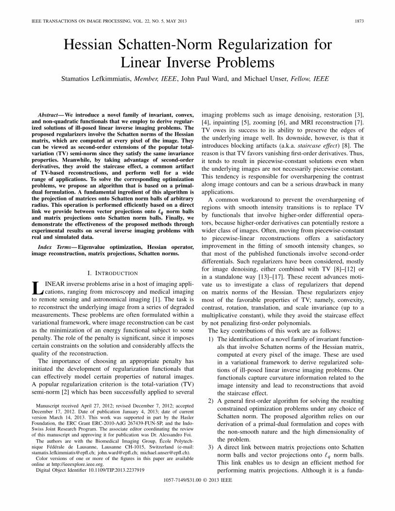
Beyond the ISNR comparisons, the effectiveness of the pro-posed method can also be visually appreciated by inspectingthe representative Face, Kids and House deblurring examplesof Figures 1–3. From these examples we can verify our initialclaims, that TV regularization leads to image reconstructions


(b)(a)

(d)(c)

Fig. 1. Restoration of the Face image degraded by Gaussian blurring andGaussian noise corresponding to a BSNR level of 15 dB. (a) Degraded image(PSNR = 21.76 dB), (b) TV result (PSNR = 25.36 dB), (c) BM3D result(PSNR = 26.51 dB), (d) H S1 result (PSNR = 26.21 dB).

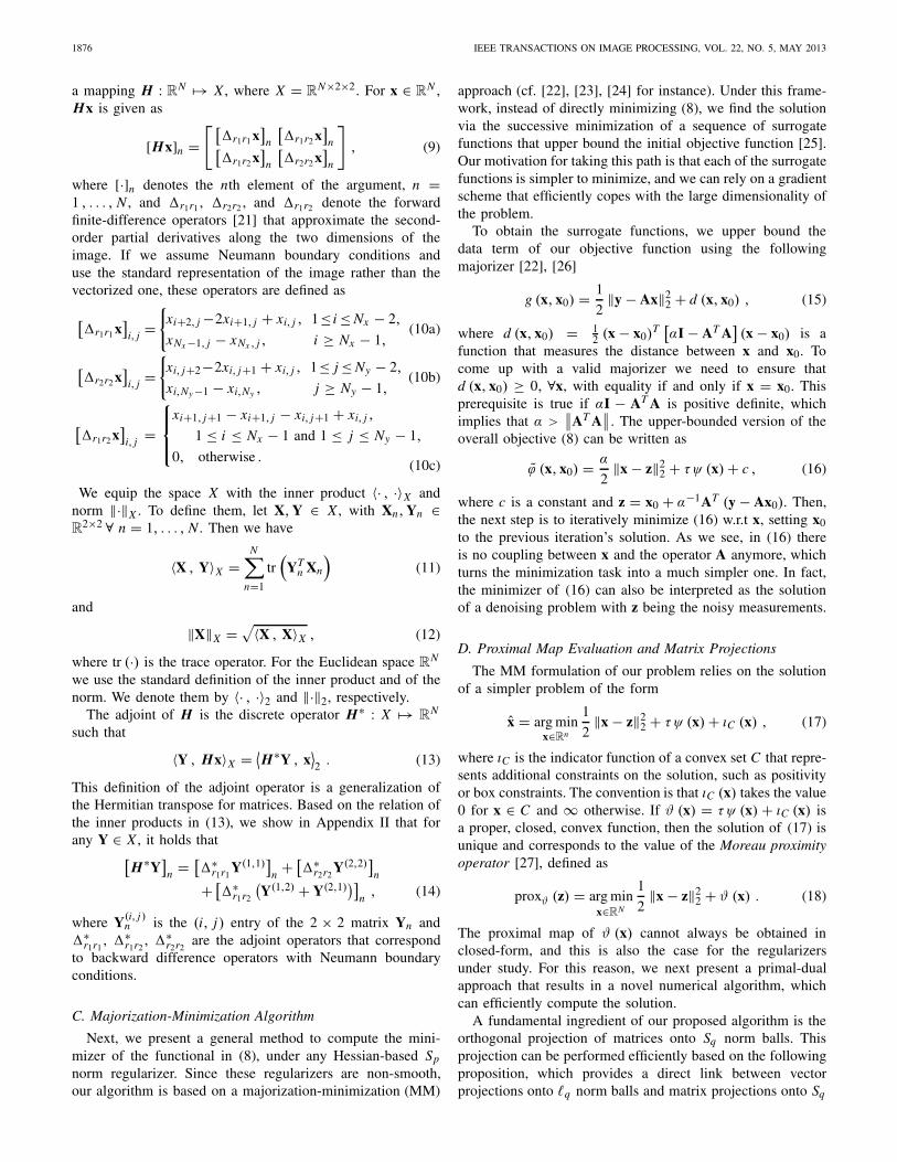
that suffer from the presence of heavy block artifacts. Theseartifacts become more evident in regions where the imageis characterized by smooth intensity transitions, and they areresponsible for shuffling details of the image and broadeningits fine structures. See for example the TV solution in Fig. 1,where the image has cartoon-like appearance. Similar blockingeffects, which are even more pronounced, appear on theHaar-based reconstructions. On the other hand, even in caseswhere the presence of the noise is significant, the Hessian-based regularizers manage to avoid introducing pronouncedartifacts and thus, they lead to reconstructions that are morefaithful representations of the original content of the image.Comparing our results with those of BM3D, we note that evenin cases where the final PSNR favors the latter reconstruction,such as in Fig. 1, our restored images have certain advantages.For example, by a careful inspection of Figs. 1 and 2, onecan clearly observe the presence of ripple-like artifacts in theBM3D solutions which do not appear in the Hessian-basedreconstructions.

C. Deblurring of Biomedical Images

Our interest in image restoration is mostly motivated bythe problem of microscopy image deblurring. In widefieldmicroscopy, the acquired images are degraded by out-of-focusblur due to the poor localization of the microscope’s PSF.This severely reduces our ability to clearly distinguish finespecimen structures. Since a widefield microscope can bemodeled in intensity as a linear space-invariant system [44],the adopted forward model in (7) is still valid and we can,thus, employ the proposed framework for the restoration ofthe underlying biomedical images.

(b)(a)

(d)(c)

Fig. 2. Restoration of the Kids image degraded by motion blurring andGaussian noise corresponding to a BSNR level of 20 dB. (a) Degraded image(PSNR = 21.84 dB), (b) Haar result (PSNR = 27.79 dB), (c) BM3D result(PSNR = 28.50 dB), (d) H S1 result (PSNR = 28.59 dB).

(b)(a)

(d)(c)

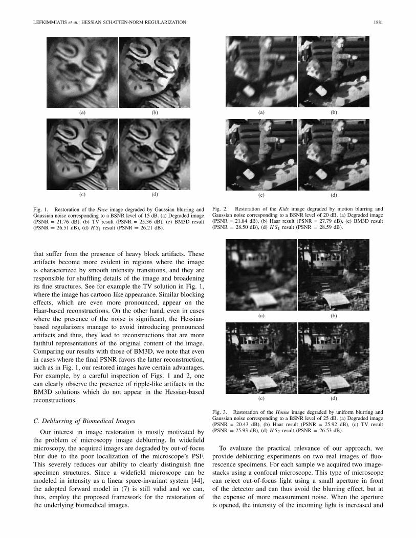
Fig. 3. Restoration of the House image degraded by uniform blurring andGaussian noise corresponding to a BSNR level of 25 dB. (a) Degraded image(PSNR = 20.43 dB), (b) Haar result (PSNR = 25.92 dB), (c) TV result(PSNR = 25.93 dB), (d) H S2 result (PSNR = 26.53 dB).

To evaluate the practical relevance of our approach, weprovide deblurring experiments on two real images of fluo-rescence specimens. For each sample we acquired two image-stacks using a confocal microscope. This type of microscopecan reject out-of-focus light using a small aperture in frontof the detector and can thus avoid the blurring effect, but atthe expense of more measurement noise. When the apertureis opened, the intensity of the incoming light is increased and


(b)(a)

(d)(c)

Fig. 4. Restoration results on a real Fluorescent Cell image of size 352 ×512. Close-up of (a) widefield image, (b) reference confocal image, (c) TVreconstruction, and (d) H S1 reconstruction. The details of this figure are betterseen in the electronic version of this paper by by zooming in on the screen.

the SNR is improved, but this time the measurements includeinterference from adjacent out-of-focus objects. In this case thefinal result is blurred and it is equivalent to an image acquiredby a “cheaper” widefield microscope. For more details on theimage acquisition we refer to [45].

The reported results refer to the restoration of the secondtype of image-stacks, with the first ones serving as visualreferences to evaluate the quality of the reconstruction. Thesize of the image-stacks for the first specimen shown inFigs. 4(a) and 4(b) are 352 × 512 × 96 while the size ofthe image stacks for the second sample shown in Figs. 5(a)and 5(b) are 512 × 512 × 16. From each of the image-stackswe obtained a single image to work with, by computing theaverage intensity with respect to the z-axis. We did the same toobtain a 2D PSF out of a standard diffraction-limited 3D PSFmodel using the nominal optical parameters of the microscope(numerical aperture, wavelength, optical zoom) [44].

In Figs. 4(c) and 4(d) we present the restored images usingTV and H S1 regularization, while in Figs. 5(c) and 5(d) weprovide the restored images using TV and H S2 regularization.From these two examples, if we compare the obtained resultswith the confocal acquisitions, we can verify that the Hessian-based solutions are quite successful in revealing the primaryfeatures of the specimens without introducing severe artifacts,as opposed to TV which oversmooths certain features andwipes out important details of the image structure. Therefore,we conclude that our regularizers can do a better job, espe-cially when one has to deal with images that consist mostlyof ridges and filament-like structures, as is often the case inbiomedical imaging.

D. Sparse Image Reconstruction

In sparse image reconstruction the observed image y isdegraded by a masking operator which randomly sets pixelvalues to zero. This operator corresponds to a diagonal matrixA whose diagonal entries are randomly set to zero or one. Werefer to this problem as sparse because in our experiments we

(b)(a)

(d)(c)

Fig. 5. Restoration results on a real Fluorescent Cell image of size512 × 512. Close-up of (a) widefield image, (b) reference confocal image,(c) TV reconstruction, and (d) H S2 reconstruction. The details of this figureare better seen in the electronic version of this paper by zooming in on thescreen.

consider masking operators that retain only 2%, 5%, 8% and10% of the initial pixel values. Note that this problem canbe considered as compressive sensing if we assume that theimage is sparse in the spatial domain.

The reported experiments are conducted on the gray-levelimages: Boat, Hill, Lena and Peppers. The masked imagesare then reconstructed using our regularizers as before plusTV and two quadratic regularizers based on the gradientand the Laplacian operators, respectively. In this setting wedo not consider any presence of noise and thus, for all theregularizers under comparison, we use the same regularizationparameter τ = 10−4. The value of τ is chosen to be small toensure that the results will be consistent, in the sense thatthe reconstruction methods will not alter the unmasked pixelvalues. However, due to the small value of the regularizationparameter, we have observed that the convergence of theminimization task for all the regularizers can be slow andthus more than 100 iterations are required. To cope withthis problem, for the non-quadratic regularizers, we apply asimple continuation scheme that significantly speeds up theconvergence: We start with a large value for τ and then wegradually decrease it to reach the chosen value. We observeexperimentally that following this strategy and using 200MFISTA iterations (we still solve the corresponding denoisingproblems using 10 iterations) we can solve the problem tohigh accuracy. Regarding the two quadratic regularizers, weminimize their objective functions using the conjugate gradientmethod [46] with a maximum of 2000 iterations.

In Table II we report the reconstruction results we obtainedfor all the employed regularization techniques. The quality ofthe reconstructions is measured in terms of PSNR. As we canobserve from this table, TV does not perform well in thisproblem and its reconstructions fall far behind, even from thetwo quadratic regularization techniques. On the other hand,our Hessian-based regularizers behave much better and in allcases they lead to estimates that outperform the other methods.


TABLE II

PSNR COMPARISONS ON SPARSE IMAGE RECONSTRUCTION FROM

RANDOM SAMPLES FOR FOUR RATIOS OF OBSERVED PIXELS

ObservedPixels % Grad. Lap. TV H S∞ H S2 H S1

Boa

t

2% 21.29 20.83 18.52 21.54 21.56 21.55

5% 22.96 22.87 21.22 23.27 23.31 23.33

8% 23.92 24.03 22.43 24.27 24.33 24.37

10% 24.51 24.67 23.00 24.92 25.00 25.06

Hill

2% 22.53 22.39 19.68 22.97 23.00 23.01

5% 24.27 24.33 22.13 24.70 24.76 24.77

8% 25.34 25.49 23.69 25.75 25.79 25.80

10% 25.90 26.07 24.52 26.29 26.34 26.35

Len

a

2% 22.33 22.79 18.89 23.23 23.34 23.38

5% 24.60 25.42 22.42 25.56 25.70 25.82

8% 25.98 26.96 24.37 26.96 27.11 27.24

10% 26.63 27.64 25.28 27.62 27.77 27.90

Pepp

ers

2% 18.58 18.50 15.68 19.20 19.27 19.32

5% 20.73 20.93 18.31 21.53 21.64 21.71

8% 21.71 22.21 19.97 22.49 22.60 22.66

10% 22.41 22.90 20.92 23.18 23.32 23.39

(b)(a)

(d)(c)

Fig. 6. Sparse reconstruction of the Peppers image from 2% observed pixels.(a) Masked image. (b) Laplacian-based quadratic result (PSNR = 18.50 dB).(c) TV result (PSNR = 15.68 dB). (d) H S1 result (PSNR = 19.32 dB).

As in the image restoration case, the H S1 regularizer leadsto the best reconstructions while the H S2 regularizer followsrather closely. In Fig. 6 we present a representative exampleof the reconstruction of the Peppers image from 2% observedpixels. From this example it is clear that TV cannot produce

TABLE III

PSNR COMPARISONS ON IMAGE INTERPOLATION AND IMAGE ZOOMING

FOR A 4× DOWNSAMPLING FACTOR

Images Grad. Lap. TV H S∞ H S2 H S1

Inte

rpol

atio

n Boat 24.03 24.19 21.90 24.43 24.45 24.45

Hill 25.48 25.62 23.31 25.83 25.84 25.83

Lena 26.57 27.74 23.95 27.79 27.89 27.92

Peppers 21.95 22.13 19.48 22.55 22.63 22.68

Zoo

min

g Boat 25.95 25.89 26.00 26.01 26.08 26.12

Hill 27.32 27.27 27.22 27.31 27.34 27.35

Lena 29.25 29.26 29.50 29.40 29.54 29.61

Peppers 24.10 24.13 24.32 24.69 24.76 24.77

an acceptable result but instead leads to a piecewise constantsolution that does not reveal any features of the image. On theother hand, both the quadratic and the proposed regularizerprovide meaningful reconstructions with the latter achieving abetter performance.

E. Image Interpolation and Image Zooming

Image interpolation and image zooming fall into the sameclass of linear inverse problems. As in the sparse imagereconstruction case, the degradation is due to a maskingoperator that zeros out some of the image pixel values.However, in these two cases the masking operator corre-sponds to subsampling and is highly structured, as opposedto the random masking operator. The difference between thetwo considered forward models is that image interpolationinvolves only the subsampling operator and therefore resultsin observed images that suffer from aliasing, while imagezooming involves additionally an antialiasing operator thatis applied to the underlying image before the subsamplingtakes place. In the last case, the matrix A can be expressed asA = SF where F corresponds to the filtering operation and Sto subsampling. Once more, we do not consider any presenceof noise and we thus use the same regularization parameter andminimization strategy as above. The experiments we presentare conducted on the same four images as in Section IV-D,using the same regularizers for a downsampling factor of 4.Finally, regarding the antialiasing filter we use a Gaussiankernel of support 9 × 9 and standard deviation σb = 1.4.

In Table III we report the obtained results and we evaluatethe quality of the estimates in terms of PSNR. Regardingthe interpolation problem we observe that TV, similarly tothe sparse image reconstruction case, does not perform welland produces the worst scores. However, its performancegets significantly better in the image zooming case wherean antialising filtering is applied. This is an indication thatTV cannot perform at a satisfactory level when the operatoracting on the image does not involve a mixing effect. Onthe other hand, the performance of the proposed regulariz-ers is more robust to the nature of the degradation oper-ator, and they lead to the best reconstructions. To have avisual performance assessment, we present in Figs. 7 and 8interpolation and zooming results on the Lena and Boat


(b)(a) (d)(c) (e)

Fig. 7. Image interpolation. Close-up of (a) High-resolution image, (b) low-resolution image, (c) Laplacian-based quadratic result (PSNR=27.74 dB), (d) TVresult (PSNR=23.95 dB), and (e) H S1 result (PSNR=27.92 dB).

(b)(a) (d)(c) (e)

Fig. 8. Image zooming. Close-up of (a) High-resolution image, (b) low-resolution image, (c) gradient-based quadratic result (PSNR = 25.95 dB), (d) TVresult (PSNR = 26.00 dB), and (e) H S2 result (PSNR = 26.08 dB).

image, respectively. These results confirm our previous con-clusions about the performance of TV and demonstrate thesuperiority of the Hessian-based regularizers over the otherregularizers.

V. CONCLUSION

In this paper we introduced a new family of convex non-quadratic regularizers that can potentially lead to improvedresults in inverse imaging problems. These regularizers incor-porate second-order information of the image and depend onthe Schatten norms of the Hessian. We further designed an effi-cient and highly parrallelizable projected gradient algorithmfor minimizing the corresponding objective functions. We alsopresented a new result that relates vector projections onto �q

norm balls and matrix projections onto Schatten norm balls.This enabled us to design a matrix-projection method, whichis a fundamental ingredient of our optimization algorithm.

The performance and practical relevance of the proposedregularization scheme was assessed for several linear inverseimaging problems, through comparisons on simulated and realexperiments with various competing methods. The results weobtained are promising and competitive both in terms of SNRimprovement and visual quality.

APPENDIX I

A. Proof of Theorem 1

By taking the domain � to be a disk, the rotation invarianceof R ( f ) implies that

R ( f (Rθ ·)) = R ( f ) (37)

where Rθ is a rotation matrix. In particular, (37) must hold forall functions, including those of the form: f (r) = αr1 + βr2,with r ∈ R

2 and α, β ∈ R. Their gradient is constant andequal to ∇ f (r) = [ α

β

] = x. Now, using f as defined above,we write the l.h.s of (37) as

R ( f (Rθ ·)) =∫�� (∇ { f (Rθ ·)} (r)) dr

=∫��

(RTθ ∇ f (Rθr)

)dr =

∫��

(RTθ x

)dr

=∫�� (|x| · uθ ′) dr , (38)

where uθ ′ = [sin

(θ ′) sin

(θ ′ + π

2

)]Tand θ ′ = θ +

sgn (α) arccos

(β√α2+β2

). Setting θ ′ = π

2 in (38) and com-

bining the result with Property (37), we immediately get that

�(x) = �(|x|) ,∀x ∈ R2 . (39)

The scaling invariance of R can be restated as

Ra ( f (a·)) = aμR ( f )∫�/a

�(∇ { f (a·)} (r)) dr = aμ∫�� (∇ f (r)) dr (40)

for some a > 0, and an exponent μ ∈ R. This property musthold for all functions, including those of the form: f (r) =αr1, with r ∈ R

2 and α ∈ R. The magnitude of their gradientis constant and equal to |∇ f (r)| = |α|. Now, using f asdefined above and the result of (39), we write (40) as∫

�/a�(a |α|) dr = aμ

∫�� (|α|) dr . (41)


Therefore, we directly have that

�(a |α|) = aν� (|α|) ,∀α ∈ R, (42)

with ν = μ+ 2. Now, we define the function

�0(α) = �(|α|)|α|ν ,∀α ∈ R (43)

which is homogeneous of degree 0. This implies that �0(α) =c, with c an arbitrary constant. Therefore, the potential func-tions � satisfying (42) are necessarily of the form: �(·) =c |·|ν .

The inverse statement of the theorem can be verified bysubstitution, using the property

∇ { f (a·)} (r) = a∇ { f } (ar) , ∀ f. (44)

B. Proof of Theorem 2

By taking the domain � to be a disk, the rotation invarianceof R ( f ), as defined in (37), must hold for all functions,including those of the form: f (r) = α2

2 r21 + β2

2 r22 + γ r1r2,

with r ∈ R2 and α, β, γ ∈ R. Their Hessian is constant and

equal to H f (r) = [ α γγ β

] = A. Now, using f as defined above,we write the l.h.s of (37) as

R ( f (Rθ ·)) =∫�� (H { f (Rθ ·)} (r)) dr

=∫��

(RTθ H f (Rθr)Rθ

)dr

=∫��

(RTθ ARθ

)dr . (45)

According to the spectral decomposition theorem, A beingsymmetric has an eigenvalue decomposition. This implies thatthere exists a rotation θ ′ such that RT

θ ′ARθ ′ = �, where � isa diagonal matrix consisting of the eigenvalues of A. Theseare denoted as λk , where k = 1, 2. Based on this observationand combining it with Property (37), we immediately get that

�(A) = �(λ1, λ2) ,∀A ∈ S2, (46)

which implies that � should be a function of the Hessianeigenvalues.

The scaling invariance of R can be restated as

Ra ( f (a·)) = aμR ( f )∫�/a

�(H { f (a·)} (r)) dr = aμ∫�� (H f (r)) dr (47)

for some a > 0, and an exponent μ ∈ R. This propertymust hold for all functions, including those of the form:f (r) = α

2 r21 + β

2 r22 , with r ∈ R

2 and α, β ∈ R. Their Hessianis constant and equal to H f (r) = [

α 00 β

]. Now, using f as

defined above and the result of (46), we write (47) as∫�/a

�(

a2α, a2β)

dr = aμ∫�� (α, β) dr . (48)

Therefore, we have that

�(

a2α, a2β)

= aμ+2�(α, β) , ∀α, β ∈ R . (49)

Now, we define the function

�0(x) = �(x)‖x‖νp

,∀x ∈ R2, (50)

where p ≥ 1 and ν = μ+22 . �0 is homogeneous of degree

0 and thus �0 (x) = �0(x/ ‖x‖p

). Therefore, the potential

functions � that satisfy (49), are necessarily of the form:�(x) = �0

(x/ ‖x‖p

) ‖x‖νp . Finally, since x represents thevector of the eigenvalues of the Hessian, its �p norm corre-sponds to the Sp norm of the Hessian itself.

The inverse statement of the theorem can be verified bysubstitution, using the property

H { f (a·)} (r) = a2 H { f } (ar) , ∀ f. (51)

APPENDIX II

A. Adjoint of the Discrete Hessian Operator

To find the adjoint of the discrete Hessian operator, weexploit the relation of the inner products of the spaces R

N

and X in (13). Using (11), we can equivalently write (13) as

N∑n=1

tr(

[Hx]Tn Yn

)=

N∑n=1

xn[H∗Y

]n . (52)

We then expand the l.h.s of (52), to obtain

N∑n=1

tr(

[Hx]Tn Yn

)=

N∑n=1

([Hx](1,1)n Y(1,1)

n +

[Hx](1,2)n

(Y(1,2)

n + Y(2,1)n

)+ [Hx](2,2)n Y(2,2)

n

)

=N∑

n=1

( [ r1r1x

]n Y(1,1)

n + [ r1r2 x

]n

(Y(1,2)

n + Y(2,1)n

)

+ [ r2r2 x

]n Y(2,2)

n

)

=N∑

n=1

xn

( [ ∗

r1r1Y(1,1)

]n

+[ ∗

r1r2

(Y(1,2) + Y(2,1)

)]n

+[ ∗

r2r2Y(2,2)

]n

). (53)

Note that Y(i, j ) corresponds to the vector that is composedof the (i, j) entries of all Yn ∈ R

2×2 matrices. Now, bycomparing the r.h.s of (52) to the r.h.s expansion of (53),it is straightforward to verify that the adjoint of the discreteHessian operator is indeed computed according to (14).

B. Proof of Proposition 1

By definition, the orthogonal projection of a matrix Y ontothe set BSq is given by

PBSq(Y) = arg min

‖X‖Sq ≤ρ‖X − Y‖2

F . (54)

Since all Schatten norms are unitarily invariant, we equiva-lently have

PBSq(Y) = arg min

‖UH XV‖Sq≤ρ

∥∥∥UH XV − UH YV∥∥∥2

F. (55)


Let us now consider the matrix Z = UH XV that is associatedwith the solution of (54). If we substitute Z in (55), then weend up with the following constrained minimization problem

PBSq(�) = arg min

‖Z‖Sq ≤ρ‖Z −�‖2

F , (56)

which corresponds to the projection of the diagonal matrix �onto the set BSq . Now, if PBSq

(�) = Z, we have

∥∥∥Z − �

∥∥∥2

F=

∥∥∥Z∥∥∥2

F+ ‖�‖2

F − 2 Re(

tr(

ZH�))

≥∥∥∥�

∥∥∥2

F

+ ‖�‖2F − 2 tr

(�T�

)=

∥∥∥� − �

∥∥∥2

F, (57)

where the inequality stems from von Neumann’s trace theo-rem [47], and � is a diagonal matrix with the singular valuesof Z. In addition, it holds that∥∥∥�

∥∥∥Sq

=∥∥∥Z

∥∥∥Sq

≤ ρ . (58)

Equations (57) and (58) immediately imply that the projectionof � equals to Z = �, i.e., a positive semidefinite diagonalmatrix. We can then perform this operation by projecting thevector, formed by the main diagonal of �, onto the convexset Bq , and then by transforming the projected vector back toa diagonal matrix. Using this fact and the relations betweenthe optimal solution of (54) and (56), we finally express theprojection of the matrix Y onto BSq as

PBSq(Y) = Udiag

(PBq (σ (Y))

)VH . (59)

C. Proof of Lemma 1

First, we present a matrix inequality that involves theSchatten norms and it will be subsequently used for the proofof the lemma. Let X, Y ∈ C

n1×n2 . Then, the inner product ofthese two matrices satisfies the following inequality

〈X , Y〉Cn1×n2 = Re(

tr(

YH X))

≤ 〈σ (X) , σ (Y)〉2

≤ ‖σ (X)‖q ‖σ (Y)‖p = ‖X‖Sq‖Y‖Sp .

(60)

The first inequality is due to von Neumann’s trace theorem[47], while the second one due to Hölder’s inequality. Thelast equality holds true from the definition of Schatten norms.

By definition, the dual norm of (20) is given by [31]:

‖�‖D = max‖�‖1,p≤1〈� , �〉X , (61)

where X , instead of RN×2×2 that is used throughout the paper,

here is assumed to be the more general linear space X =C

N×n1×n2 . We consider the inequality

〈� , �〉X =N∑

n=1

Re(

tr(�H

n �n

))≤

N∑n=1

‖�n‖Sq‖�n‖Sp ,

(62)which immediatelly follows from inequality (60). Now, byintroducing the vectors ω =

(‖�1‖Sq , ‖�2‖Sq , . . . , ‖�N ‖Sq

)

and ψ =(‖�1‖Sp , ‖�2‖Sp , . . . , ‖�N ‖Sp

), and applying

once again Hölder’s inequality, we get

N∑n=1

‖�n‖Sq‖�n‖Sp = 〈ω , ψ〉2 ≤ ‖ω‖∞ ‖ψ‖1

= ‖�‖∞,q ‖�‖1,p . (63)

From the definition of the dual norm (61) and the inequal-ities (62) and (63) we conclude that ‖�‖D ≤ ‖�‖∞,q . Toprove that ‖�‖D = ‖�‖∞,q , we next show that for each� we can find a � satisfying ‖�‖1,p = 1, and for which〈� , �〉X = ‖�‖∞,q . To that end, let k be any index in the set{

arg max1≤n≤N ‖�n‖Sq

}and �k = Uk�kVH

k be the singularvalue decomposition of �k . Then, we set �n = O for all nexcept for n = k for which we have

�k = UkEVHk , (64)

where

E(i, j ) =(�(i, j )k

)q−1

‖�k‖q−1Sq

, (65)

and �(i, j )k corresponds to the (i, j)-th entry of the matrix �k ∈

Dn1×n2 . Now, we have that

〈� , �〉X =N∑

n=1

Re(

tr(�H

n �n

))= Re

(tr(�H

k �k

))

= tr(

EH�k

)=

min(n1,n2)∑i=1

(�(i,i)k

)q

‖�k‖q−1Sq

= ‖�k‖Sq = ‖�‖∞,q . (66)

Furhermore, for the mixed norm ‖�‖1,p = ‖�k‖Sp it holds

‖�‖1,p =⎛⎝min(n1,n2)∑

i=1

(E(i,i)

)p

⎞⎠

1/p

=

(min(n1,n2)∑

i=1

(�(i,i)k

)q) q−1

q

‖�k‖q−1Sq

=‖�k‖q−1

Sq

‖�k‖q−1Sq

= 1 (67)

which completes the proof of the lemma.

D. Proof of Proposition 2

For any pair of variables � ,� ∈ X we have

‖∇s (�)− ∇s (�)‖X = ‖τH (V (�)− V (�))‖X

≤ τ ‖H‖ ‖V (�)− V (�)‖2

≤ τ ‖H‖ ∥∥τH∗ (�− �)∥∥

2

≤ τ 2 ‖H‖ ∥∥H∗∥∥ ‖�− �‖X

= τ 2 ‖H‖2 ‖�− �‖X , (68)

where V (�) = PC(z − τH∗�

). Note that, the first and

third inequalities follow from the relation between the norms,defined in the spaces X and R

N , and the induced operator


norm, i.e., ‖Hx‖X ≤ ‖H‖ ‖x‖2, while the second one holdsbecause the projection operator PC onto the convex set C ⊆R

N , is firmly nonexpansive [48, Proposition 4.8]. This meansthat

‖PC (x)− PC (y)‖2 ≤ ‖x − y‖2 ∀ x, y ∈ RN . (69)

To compute an upper bound of ‖H‖, we exploit that ‖H‖2 =∥∥H∗ H∥∥ [49] (a general property of bounded linear operators),

and we get∥∥H∗ Hx

∥∥2 = ∥∥( ∗

r1r1 r1r1 + 2 ∗

r1r2 r1r2 + ∗

r2r2 r2r2

)x∥∥

2

≤(∥∥ r1r1

∥∥2 + 2∥∥ r1r2

∥∥2 + ∥∥ r2r2

∥∥2)

‖x‖2 .

(70)

Now, using the definitions of the second-order differentialoperators in (10), it is easy to show that each of

∥∥ r1r1

∥∥,∥∥ r1r2

∥∥ and∥∥ r2r2

∥∥ is smaller than or equal to 4. Thisimmediately implies that ‖H‖ ≤ 8 and, hence, an upper boundof the Lipschitz constant of ∇s (�) will be L (s) ≤ τ 2 ‖H‖2 ≤64τ 2.

ACKNOWLEDGMENT

The authors would like to acknowledge Jean-Charles Bari-taux and Pouya Tafti for fruitful discussions. They would alsolike to thank the anonymous reviewers and the associate editorfor their useful comments and suggestions.

REFERENCES

[1] M. Bertero and P. Boccacci, Introduction to Inverse Problems in Imag-ing. Boca Raton, FL: CRC Press, 1998.

[2] L. Rudin, S. Osher, and E. Fatemi, “Nonlinear total variation based noiseremoval algorithms,” Phys. D, vol. 60, nos. 1–4, pp. 259–268, 1992.

[3] J. Bioucas-Dias, J. Oliveira, and M. Figueiredo, “Total variation-basedimage deconvolution: A majorization—minimization approach,” in Proc.Int. Conf. Acoust., Speech Signal Process., vol. 2. Toulouse, France,2006, pp. 861–864.

[4] A. Beck and M. Teboulle, “Fast gradient-based algorithms for con-strained total variation image denoising and deblurring problems,” IEEETrans. Image Process., vol. 18, no. 11, pp. 2419–2434, Nov. 2009.

[5] T. F. Chan and J. Shen, “Mathematical models for local nontextureinpaintings,” SIAM J. Appl. Math., vol. 62, no. 3, pp. 1019–1043, 2002.

[6] A. Chambolle, “An algorithm for total variation minimization andapplications,” J. Math. Imag. Vis., vol. 20, nos. 1–2, pp. 89–97, 2004.

[7] M. Lustig, D. Donoho, and J. M. Pauly, “Sparse MRI: The application ofcompressed sensing for rapid MR imaging,” Magn. Reson. Med., vol. 58,no. 6, pp. 1182–1195, 2007.

[8] T. Chan, A. Marquina, and P. Mulet, “High-order total variation-basedimage restoration,” Soc. Ind. Appl. Math. J. Sci. Comput., vol. 22, no. 2,pp. 503–516, 2000.

[9] A. Chambolle and P.-L. Lions, “Image recovery via total variationminimization and related problems,” Numer. Math., vol. 76, no. 2,pp. 167–188, 1997.

[10] M. Lysaker and X.-C. Tai, “Iterative image restoration combining totalvariation minimization and a second-order functional,” Int. J. Comput.Vis., vol. 66, no. 1, pp. 5–18, 2006.

[11] T. F. Chan, S. Esedoglu, and F. E. Park, “Image decomposition com-bining staircase reduction and texture extraction,” J. Visual Commun.Image Represent., vol. 18, no. 6, pp. 464–486, 2007.

[12] S. Setzer, G. Steidl, and T. Teuber, “Infimal convolution regularizationswith discrete �1-type functionals,” Commun. Math. Sci., vol. 9, no. 3,pp. 797–827, 2011.

[13] Y.-L. You and M. Kaveh, “Fourth-order partial differential equationsfor noise removal,” IEEE Trans. Image Process., vol. 9, no. 10,pp. 1723–1730, Oct. 2000.

[14] M. Lysaker, A. Lundervold, and X.-C. Tai, “Noise removal using fourth-order partial differential equation with applications to medical magneticresonance images in space and time,” IEEE Trans. Image Process.,vol. 12, no. 12, pp. 1579–1590, Dec. 2003.

[15] G. Steidl, “A note on the dual treatment of higher-order regularizationfunctionals,” Computing, vol. 76, nos. 1–2, pp. 135–148, 2006.

[16] J. Yuan, C. Schnörr, and G. Steidl, “Total-variation based piecewiseaffine regularization,” in Proc. Sec. Int. Conf. Scale Space MethodsVariat. Methods Comput. Vis., 2009, pp. 552–564.

[17] K. Bredies, K. Kunisch, and T. Pock, “Total generalized variation,” SIAMJ. Imaging Sci., vol. 3, no. 3, pp. 492–526, 2010.

[18] R. Bhatia, Matrix Analysis. New York: Springer-Verlag, 1997.[19] S. Lefkimmiatis, A. Bourquard, and M. Unser, “Hessian-based norm

regularization for image restoration with biomedical applications,” IEEETrans. Image Process., vol. 21, no. 3, pp. 983–995, Mar. 2012.

[20] P. C. Hansen, J. G. Nagy, and D. P. O’Leary, Deblurring Images:Matrices, Spectra, and Filtering. Philadelphia, PA: SIAM, 2006.

[21] J. E. Denis and R. B. Schnabel, Numerical Methods for UnconstrainedOptimization and Nonlinear Equations. Philadelphia, PA: SIAM, 1983.

[22] I. Daubechies, M. Defrise, and C. De Mol, “An iterative thresholdingalgorithm for linear inverse problems with a sparsity constraint,” Com-mun. Pure Appl. Math., vol. 57, no. 11, pp. 1413–1457, 2004.

[23] M. Figueiredo, J. Bioucas-Dias, and R. Nowak, “Majorization—minimization algorithms for wavelet-based image restoration,” IEEETrans. Image Process., vol. 16, no. 12, pp. 2980–2991, Dec. 2007.

[24] A. Beck and M. Teboulle, “A fast iterative shrinkage-thresholdingalgorithm for linear inverse problems,” SIAM J. Imag. Sci., vol. 2, no. 1,pp. 183–202, 2009.

[25] D. Hunter and K. Lange, “A tutorial on MM algorithms,” Amer. Stat.,vol. 58, no. 1, pp. 30–37, 2004.

[26] M. Zibulevsky and M. Elad, “L1-L2 optimization in signal and imageprocessing,” IEEE Signal Process. Mag., vol. 27, no. 3, pp. 76–88, May2010.

[27] P. L. Combettes and V. R. Wajs, “Signal recovery by proximalforward-backward splitting,” Multiscale Model. Simul., vol. 4, no. 4,pp. 1168–1200, 2005.

[28] A. Lewis and J. Malick, “Alternating projections on manifolds,” Math.Oper. Res., vol. 33, no. 1, pp. 216–234, 2008.

[29] F. Bach, R. Jenatton, J. Mairal, and G. Obozinski, “Optimization withsparsity-inducing penalties,” Found. Trends Mach. Learn., vol. 4, no. 1,pp. 1–106, 2011.

[30] S. Suvrit, “Fast projections onto �1,q -norm balls for grouped featureselection,” in Proc. Eur. Conf. Mach. Learn. Knowl. Discovery Data-bases, vol. 3. 2011, pp. 305–317.

[31] R. T. Rokcafellar, Convex Analysis. Princeton, NJ: Princeton Univ. Press,1970.

[32] Y. Nesterov, “A method for solving a convex programming problemwith convergence rates O(1/k2),” Soviet Math. Dokl, vol. 27, no. 2,pp. 372–376, 1983.

[33] J. Liu and J. Ye, “Efficient �1/�q norm regularization,” 2010, Arxivpreprint arXiv: 1009.4766

[34] J.-F. Cai, E. J. Candes, and Z. Shen, “A singular value thresholdingalgorithm for matrix completion,” SIAM J. Optim., vol. 20, no. 4,pp. 1956–1982, 2008.

[35] S. Ma, D. Godfarb, and L. Chen, “Fixed point and Bregman iterativemethods for matrix rank minimization,” Math. Program., vol. 128, no. 1,pp. 321–353, 2011.

[36] G. A. Watson, “Characterization of the subdifferential of some matrixnorms,” Linear Algebra Appl., vol. 170, pp. 33–45, Jun. 1992.

[37] D. L. Donoho, “Denoising by soft-thresholding,” IEEE Trans. Inf.Theory, vol. 41, no. 3, pp. 613–627, May 1995.

[38] E. Candes and J. Romberg, “Practical signal recovery from randomprojections,” Proc. SPIE, vol. 5674, pp. 76–86, Jan. 2005.

[39] I. Daubechies, M. Fornasier, and I. Loris, “Accelerated projected gradientmethod for linear inverse problems with sparsity constraints,” J. FourierAnal. Appl., vol. 14, nos. 5–6, pp. 764–792, 2008.

[40] E. Van De Berg, M. Friedlander, and K. Murphy, “Group sparsity vialinear-time projection,” Dept. Comput. Sci., Univ. British Columbia,Vancouver, BC, Canada, Tech. Rep. TR-2008-09, 2008.

[41] J. Duchi, S. Shalev-Shwartz, Y. Singer, and T. Chandra, “Efficientprojections onto the �1-ball for learning in high dimensions,” in Proc.25th Int. Conf. Mach. Learn., 2008, pp. 272–279.

[42] K. Dabov, A. Foi, V. Katkovnik, and K. Egiazarian, “Image restorationby sparse 3D transform-domain collaborative filtering,” Proc. SPIE,vol. 6812, p. 681207, Mar. 2008.


[43] I. Selesnick and M. Figueiredo, “Signal restoration with overcompletewavelet transforms: Comparison of analysis and synthesis priors,” Proc.SPIE, vol. 7446, p. 74460D, Aug. 2009.

[44] C. Vonesch, F. Aguet, J.-L. Vonesch, and M. Unser, “The coloredrevolution of bioimaging,” IEEE Sig. Process. Mag., vol. 23, no. 3,pp. 20–31, May 2006.

[45] C. Vonesch and M. Unser, “A fast thresholded Landweber algorithmfor wavelet-regularized multidimensional deconvolution,” IEEE Trans.Image Process., vol. 17, no. 4, pp. 539–549, Apr. 2008.

[46] J. R. Shewchuk. (1994). An Introduction to the Conjugate Gra-dient Method without the Agonizing Pain [Online]. Available:http://www.cs.cmu.edu/∼jrs/jrspapers.html

[47] L. Mirsky, “A trace inequality of John von Neumann,” Monatshefte FurMathematik, vol. 79, no. 4, pp. 303–306, 1975.

[48] H. H. Bauschke and P. L. Combettes, “Convexity and nonexpansiveness,”in Convex Analysis and Monotone Operator Theory in Hilbert Spaces,J. M. Borwein and P. Borwein, Eds. New York: Springer-Verlag, 2011,pp. 59–74.

[49] V. Hutson, J. S. Pym, and M. J. Cloud, Applications of FunctionalAnalysis and Operator Theory, 2nd ed. New York: Elsevier, 2005.

Stamatios Lefkimmiatis (S’08–M’11) received theM.Sc. degree in computer engineering and informat-ics (hons.) from the University of Patras, Patras,Greece, in 2004, and the Ph.D. degree from theNational Technical University of Athens, Athens,Greece, in 2009.

He has been a Research Scientist with the Bio-medical Imaging Group, Swiss Federal Institute ofTechnology, Lausanne, Switzerland, since 2010. Hiscurrent research interests include image analysis,statistical modeling, and image reconstruction using

convex optimization techniques.

John Paul Ward received the B.S. degree in math-ematics from the University of Georgia, Athens,and the Ph.D. degree in mathematics from TexasA&M University, College Station, in 2005 and 2010,respectively.

He is currently a Post-Doctoral Researcher withthe Biomedical Imaging Group, Swiss Federal Insti-tute of Technology, Lausanne, Switzerland.

Michael Unser (M’89–SM’94–F’99) is a Professorand Director of the École Polytechnique Fédérale deLausanne’s Biomedical Imaging Group, Lausanne,Switzerland. From 1985 to 1997, he was with theBiomedical Engineering and Instrumentation Pro-gram, National Institutes of Health, Bethesda, MD,conducting research on bioimaging and heading theImage Processing Group. He has published over200 journal papers. His current research interestsinclude biomedical image processing, sampling the-ories, multiresolution algorithms, wavelets, and the

use of splines for image processing.He was a EURASIP Fellow in 2009 and a member of the Swiss Academy

of Engineering Sciences. He is the recipient of several international prizes,including three IEEE-SPS Best Paper Awards and two Technical AchievementAwards from the IEEE (2008 SPS and EMBS 2010).

ieee transactions on image processing, …big · hessian schatten-norm regularization for linear...

Documents