bootstrapped policy gradient for difficulty adaptation in

Bootstrapped Policy Gradient for Difficulty Adaptation inIntelligent Tutoring Systems

Yaqian Zhang

Nanyang Technological University

Singapore, Singapore

[email protected]

Wooi-Boon Goh

Nanyang Technological University

Singapore, Singapore

[email protected]

ABSTRACTOne challenge for an intelligent interactive tutoring agent is to

autonomously determine the difficulty levels of the questions pre-

sented to the users. This difficulty adaptation problem can be for-

mulated as a sequential decision making problem which can be

solved by Reinforcement learning (RL) methods. However, the cost

of taking an action is an important consideration when applying

RL in real-time responsive application involving human in the loop.

Sample efficient algorithms are therefore critical for such applica-

tions, especially when the action space is large. This paper proposes

a bootstrapped policy gradient (BPG) framework, which can incor-

porate prior knowledge into policy gradient to enhance sample

efficiency. The core idea is to update the summed probability of

a set of related actions rather than a single action at gradient es-

timation sample. A sufficient condition for unbiased convergence

is provided and proved. We apply the BPG to solve the difficulty

adaptation problem in a challenging environment with large action

space and short horizon, and it achieves fast and unbiased con-

vergence both in theory and in practice. We also generalize BPG

to multi-dimensional continuous action domain in general actor-

critic reinforcement learning algorithms with no prior knowledge

required.

KEYWORDSReinforcement Learning; Multi-arm Bandit; Policy Gradient; Intel-

ligent Tutoring Systems; Bootstrapped Policy Gradient

ACM Reference Format:Yaqian Zhang and Wooi-Boon Goh. 2019. Bootstrapped Policy Gradient

for Difficulty Adaptation in Intelligent Tutoring Systems. In Proc. of the18th International Conference on Autonomous Agents and Multiagent Systems(AAMAS 2019), Montreal, Canada, May 13–17, 2019, IFAAMAS, 9 pages.

1 INTRODUCTIONWith the increasing adoption of the Massive Open Online Courses

(MOOC), there is an important need for online education systems

to take into account individual differences so that contents and

assessments can be personalized to match users who have diverse

backgrounds and ability levels. The “flow theory” [6] suggests that

the present challenge must be optimally set to a person’s ability

in order to avoid frustration when the task is too difficult and

boredom when it is trivial. On the educational front, the theory

of “proximal development zone” [1] suggests that learning gain

is optimal when the difficulty level matches the student’s ability.

Proc. of the 18th International Conference on Autonomous Agents and Multiagent Systems(AAMAS 2019), N. Agmon, M. E. Taylor, E. Elkind, M. Veloso (eds.), May 13–17, 2019,Montreal, Canada. © 2019 International Foundation for Autonomous Agents and

Multiagent Systems (www.ifaamas.org). All rights reserved.

However, traditional educational systems usually employ hand-

crafted rules [18], which can become difficult to determine and

maintain if the choices of task are large and the user base is diverse.

Related research works have applied RL for interaction optimiza-

tion in Human Computer Interaction (HCI), where the RL agent

interacts with the user to make some interactive decisions with

the aim of enhancing user experience. For instance, Markov deci-

sion process (MDP) or partially observed Markov decision process

(POMDP) frameworks have been used to support the sequential

decision-making, such as sequencing seven education concepts

[13], choosing from two pedagogical strategies [3] and selecting

from three display interventional messages [23]. In these applica-

tions, the action space is small, often less than 10. When it comes

to a larger action space, MDP/POMDP suffer from the curse of

dimensionality. In the intelligent tutoring system, there could be

hundreds or even thousands of candidates in the questions bank

[10, 17, 24]. In these large action space cases, Multi-armed Bandit

(MAB) or contextual MAB frameworks are usually employed as

more scalable approaches [5, 10, 12]. The most similar work to ours

is Maple (Multi-Armed Bandits based Personalization for Learning

Environments) [22] which also formalizes difficulty adaptation in

the framework of MAB. This work heuristically uses the prior in-

formation of difficulty ranking to improve the efficacy for difficulty

adjustment. However, despite the promising empirical results, no

theoretical guarantee for convergence is provided and it is unclear

whether the algorithm introduces bias to the optimal question. Gen-

erally, compared to the numerous studies of RL in other domains,

like control systems or game-playing (Atari games, board games),

the work of applying RL to benefit human interaction is much more

limited.

A major challenge in applying RL algorithms to real-world in-

teractive application lies in sample efficiency. Value function-based

reinforcement learning methods [15, 19, 30], such as (deep) Q-learning, have been considered as sample efficient since it can

train on off-policy data with experience replay technique [19]. Nev-

ertheless, a suitable exploration policy [2, 7, 16], such as ϵ-greedy,Thompson sampling, is required in off-policy learning for efficient

exploration. The trade-off between exploration and exploitation

is a tricky issue [4]. As the action space becomes larger, efficient

exploration becomes more challenging. Generally, the convergence

of value function-based algorithms is not guaranteed [8, 26, 29].

Compared to value function-based method, policy gradient-based

methods [20, 21, 27, 31] exhibit more stable convergence both in

theory and in practice because these methods directly estimate the

gradient of RL objective [29]. However, a main limitation for policy

gradient methods is that they are severely sample inefficient due

to the on-policy learning and high variance in gradient estimation

Session 3B: Socially Intelligent Agents AAMAS 2019, May 13-17, 2019, Montréal, Canada

711

[21, 29]. To achieve stable iterative policy optimization, a large

batch size needs to be employed. For example, for continuous con-

trol task in Mujoco simulator [28], the common choice of batch size

is often above 1000. However, responsive interactive application

cannot afford to use such large batch sizes as it will result in slow

adaptation to the user. In fact, instead of batch update, incremental

method which updates the parameters immediately after receiv-

ing a user feedback, is often used to ensure good user experience

[5, 10, 22]. Therefore, this paper investigates how to make the pol-

icy gradient method feasible and stable for small batch size update.

Specifically, we study how policy gradient can be bootstrapped by

priori information to be applied in the environments with short

exploration horizon T and large action space A (T ≪ A).This paper makes a threefold contribution. Firstly, we proposed

a general framework (BPG) for incorporating the prior informa-

tion of action relations into policy gradient to achieve stable policy

optimization even with small batch size. A sufficient condition is

identified to guarantee unbiased convergence while employing BPG.

Secondly, based on this framework, we developed a BPG-based dif-

ficulty adaptation scheme which can be applied in the intelligent

tutoring systems with large action space and short horizon. Thirdly,

we studied the generalization of BPG for multi-dimensional contin-

uous action space in the general actor-critic reinforcement learning

methods.

2 BACKGROUND2.1 Problem FormulationConsider a multi-armed bandits framework defined by ⟨A,R⟩,

where A = {a1, ...,aA} is a finite set of actions and R : A → R is

the reward function. The agent samples action ai from a stochastic

policy πθ (a) : A → [0, 1] parameterized by θ . The environment

generates a reward rai from a unknown probability rai ∼ P(r |ai ),indicating how good the action is. The goal of the agent is to maxi-

mize one-step MDP return as Eq (1).

maxθ J (θ ) = maxθ Eai∼πθ [rai ] (1)

A commonly used policy is the softmax policy πθ (ai ) =ewi (θ )

Σk ewk (θ )

with w ∈ RA as the softmax weights and thus ewi (θ ) ∝ πθ (ai ).(To simplify notation,wi (θ ) will be frequently denoted aswi ). The

softmax weights can be a more complex functionw(θ,ϕ), such as

neural network, w.r.t θ and the action features ϕ(ai ).The problem of difficulty adaptation can be formulated in the

context of MAB by taking questions as actions and the suitability

of a question for a user as the reward. Specifically, we consider a

setting with two actors: a user who is interacting with a system to

complete a number of questions; and an agent selecting questions

from a number of question candidates A = {a1, ...,aA} aiming to

suitably challenge the user. At each time step, t ∈ [1, ...,T ](T ≪ A),the agent selects a question ai from question bank A and the user

engages with the question and then the agent receives an observa-

tion of grade дai and a scalar value of reward rai . The grade д is

negatively related to difficulty. If the grade is too high, the question

is too easy for the user and vice verse. A target grade valueG ∈ R is

specified in advance to indicate the state of the user being suitably

challenged. The reward indicates the suitability of this question for

the user, which is measured by the distance of the current grade to

the target grade Rai = −|дai −G |. A ranking of questions Da ∈ RM

is known in advance. D(ak ) < D(ai ) refers to task ak is easier than

ai . In summary, the input is a target performance G and a known

task difficulty ranking Da,a ∈ A. The agent outputs a question to

the user at each time step with the goal of keeping the user grade

at the target value as close as possible, i.e. selecting the optimal

action with highest reward.

2.2 Policy GradientBased on stochastic policy gradient theorem [27], the gradient of the

objective function in Eq (1) can be reduced to a simple expectation,

which can be obtained through sample-based estimates as shown

in Eq (2). An intuitive understanding of this method is that the

parameter is adjusted to update the exploration probability of an

action based on the reward it receives. When an action leads to a

high reward, the policy parameter will be adjusted to select this

action more often.

∇θ J (θ ) = Eai∼πθ [ra i∇θ logπθ (ai )] (2)

As mentioned earlier, policy gradient method suffers from high

variance in gradient estimation and thus necessities a large batch

size for stable policy optimization. To better illustrate why large

batch size is necessary, we show exactly how the softmax weights

are updated in Eq (2). In the true gradient, the softmax weight of

an action will be increased if and only it has better-than-average

reward, i.e. ∇wk J (θ ) = πθ (ak )(rak − Ea∼πθ [ra ]). However, in the

one-sample estimation of the gradient, as long as the sampled re-

ward rai is positive, the softmaxweight of the sampled action ai will

always be increased, i.e. ∇wi J (θ )|ai = (1 − πθ (ai ))rai , and all the

other actions’ weights will be always decreased, i.e. ∇w j J (θ )|ai =−πθ (aj )rai ,aj , ai . With infinite samples, all inaccuracy update

will be canceled off and eventually an accurate estimation of gra-

dient can be obtained, i.e. ∇wk J (θ ) = Eai∼πθ [∇wk J (θ )|ai ]. But inrealistic scenarios, we do not have infinity samples to estimate one

gradient step. Therefore, many researchers have studied how to

reduce the variance in estimation so that a small number of samples

can achieve an accurate estimation of gradient [8, 11, 21, 29, 31, 32].

In these works, new score functions f (a) are proposed to replace

the raw reward ra in the gradient estimation sample in Eq (2), i.e.

∇θ J (θ ) = Eai∼πθ [f (ai )∇θ logπθ (ai )]. The score functions f (ai )are constructed by subtracting the reward with some baselines. If

the baselines are independent of actions, i.e. f (ai ) = ra i −B, then de-spite the value change at individual gradient estimation sample, the

overall expectation of the gradient estimation samples remains the

same because Eai∼πθ [B∇θ logπθ (ai )] = 0. In other words, adding

any action-independent baseline will not introduce any bias to the

gradient direction [14, 26]. In terms of the exact value of baseline, a

common choice is the average reward B = Ea∼πθ [ra ]. In this way,

at each gradient estimation sample, the sampled action’s probabil-

ity will be increased only when it receives a better-than-average

reward instead of a positive reward as in the original case in Eq (2).


712

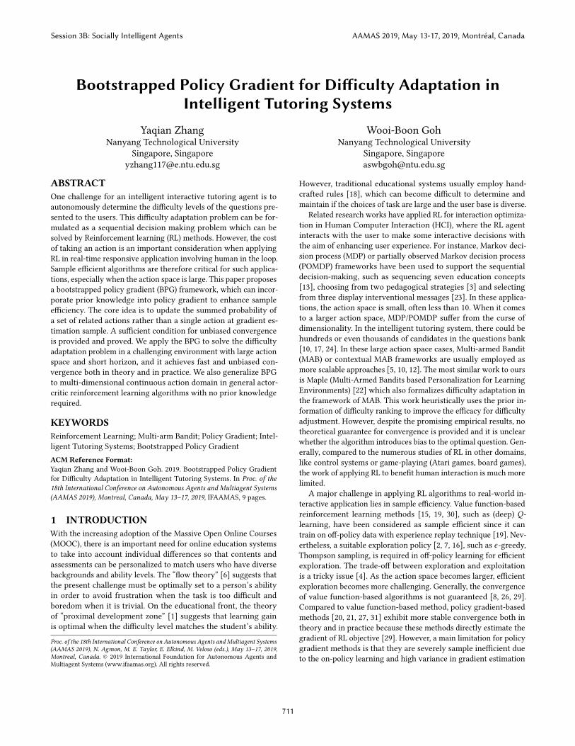
Figure 1: Policy Gradient with batch size equal to one

3 SAMPLE EFFICIENT POLICY GRADIENT3.1 MotivationTo apply policy gradient into the problem with short horizon Tand large action space A (T ≪ A), we examine policy gradient

for incremental update with batch size equal to one. We notice

that policy gradient method would fail under this scenario even

with the above variance reduction scheme. Note that in individ-

ual policy gradient estimation sample, the softmax weight of the

sampled action is updated in one direction and all the other ac-

tions’ updated in the opposite direction. And the above variance

reduction scheme does not change this fact. As a result, the agent

is still susceptible to being stuck at the sampled action. Specifically,

if the sampled action has better-than-average f (ai ) > 0, only the

sampled action’s softmax weight will be increased and thus its

probability is guaranteed to be enhanced. In fact, its probability

increase over other actions is in exponential scale w.r.t the step size

α , sinceπ t+1θ (ai )π t+1θ (ak )

=π tθ (ai )π tθ (ak )

eαxi (ak ), where xi (ak ) = ∇wi J (θ )|ai −

∇wk J (θ )|ai = f (ai )(1 + πtθ (ak ) − π tθ (ai )) and xi (ak ) > 0 if f (ai ) >

0. Hence, the step size needs to be kept very small when receiv-

ing positive score function values f (ai ) > 0. For the case with

f (ai ) < 0, the issue of being stuck in sub-optimal solutions can

be alleviated since the agent does not increase a single action’s

softmax weight but increases for multiple actions i.e. all ak , ai .However, policy gradient would still be unfeasible in our problem

with short horizon T and large action space A (T ≪ A), due to the

fact the number of exploration steps T needed in this method have

to be greater than the action numbers A. Because if the method

does not use any prior knowledge of the actions, then it has to see

all the actions, at least once, to decide which one is the best. Fig

1 shows the probability of the optimal target action of applying

incremental policy gradient in two toy problems with 20 actions

and fixed rewards uniformly distributed from [-0.5,0.5] for problem

1 and [-1,0] for problem 2. Results show that for Problem 1, the

step size has to be kept small to avoid being stuck in sub-optimal.

As a result, it needs nearly 10000 steps to converge, even with this

simple problem. Large step size can be used in problem 2 to achieve

faster convergence but the convergence steps is bounded at the

number of actions (log 20 ≈ 1.3), no matter how large the step size

is.

In the next section, we introduce a new method called Boot-

strapped Policy Gradient (BPG), which incorporates prior infor-

mation of action relationship into the policy gradient to bootstrap

policy optimization. The proposed method can achieve stable and

faster convergence to the target optimal action (without actually

seeing all the actions) and can thus be applied in problems with

short horizon and large action space.

3.2 Bootstrapped Policy GradientConsider a prior information which states certain actions are likely

to have higher/lower reward than others. We will first discuss how

to incorporate such prior information into policy gradient with

unbiased convergence guarantee (in section 3.2 and 3.3) and then

discuss how such information can be obtained in practice (in section

4 and 5).

We propose a novel idea of updating the probability of a setof actions instead of a single action in gradient sample. Let X+aidenote better action set, which includes the actions that might

be better than ai and X−ai denote a worse action set, which con-

tains the worse actions than ai . The bootstrapped policy gradi-

ent1formalized in Eq (3) increases the probability of the better

action set

⌢π+

θ (ai ) := Σak ∈X+aiπθ (ak ) and decreases the probability

⌢π−

θ (ai ) := Σak ∈X−aiπθ (ak ) of worse action set.

˜∇θ J (θ ) = Eai∼πθ [|rai |(∇θ log⌢π+

θ (ai ) − ∇θ log⌢π−

θ (ai ))] (3)

Compared to traditional policy gradient, the proposed method

enjoys several advantages. Firstly, in each gradient sample, the

agent does not raise a single action’s probability weights but that

of a set of actions’. Thus it is more stable and less likely to be stuck

with a certain action, regardless of the sign of the reward. This can

also be shown in the softmax weights˜∇wk J (θ ) =

πθ (ak )⌢π+

θ (ai )|rai |,ak ∈

X+ai and˜∇wk J (θ ) = −

πθ (ak )⌢π

−

θ (ai )|rai |,ak ∈ X−

ai , where the weight

change direction no longer relies on whether the action is the

sampled action and the sign of the reward. This property makes

it possible for BPG to stably update policy even with batch size

equal to one. Secondly, we can see in BPG the "worse" action’s

probability can be decreased without actually exploring it and the

"better" action’ probability can be increased before it has been

selected. It is this property that makes it possible for BPG to find

the best action without exhaustively trying every action. In the

interactive application, this means that the agent can eliminate

some undesirable choices without actually exposing them to the

users and use the limited exploration steps to focus more on the

promising ones.

In spite of the promising properties of the BPG, an immediate

question is how to ensure that the surrogate gradient can still lead

to the target optimal action, given that the gradient direction has

been altered. Notably the performance of BPG is dependent on the

"quality" of the "better/worse action set". We therefore investigate

how to ensure the proposed surrogate gradient method to converge

at the original optimal action and what kind of constraints on "bet-

ter/worse action set" are required for such unbiased convergence.

3.3 Convergence AnalysisWe define the original target action(s) as a∗ := argmax ra . Thenthe goal is to make the surrogate gradient converge to a policy,

where πθ (ak ) = 0,∀ak , a∗. For convenience, we define A+θ :=

1In the case of

⌢π θ (ai ) = 0, the gradient update is set to be zero by letting

⌢π θ (ai ) to

be equal to a constant.


713

{∀ai |⌢π+

θ (ai ) > 0} and A−θ := {∀ai |

⌢π−

θ (ai ) > 0}. Then from Eq (3)

we have:

˜∇θ J (θ ) =∑

ai ∈A+θ

πθ (ai )|rai |∇θ log⌢π+

θ (ai )

−∑

ai ∈A−θ

πθ (ai )|rai |∇θ log⌢π−

θ (ai )

=∑

ai ∈A+θ

πθ (ai )|rai |⌢π+

θ (ai )∇θ

⌢π+

θ (ai ) −∑

ai ∈A−θ

πθ (ai )|rai |⌢π−

θ (ai )∇θ

⌢π−

θ (ai )

The first equality uses the definition of expectation. The second

equality uses the property of ∇θπθ (ai ) = πθ (ai )∇θ logπθ (ai ).

We define h+θ (ai ) :=

πθ (ai )⌢π+

θ (ai )|rai |,

⌢π+

θ (ai ) > 0

0,⌢π+

θ (ai ) = 0

(likewise for

h−θ (ai )). Following these definitions, we have:

˜∇θ J (θ ) =∑ai

hθ (ai )∇θ⌢π+

θ (ai ) −∑ai

h−θ (ai )∇θ⌢π+

θ (ai )

=∑ai

h+θ (ai )∑

ak ∈X+ai

∇θπθ (ak ) −∑ai

h−θ (ai )∑

ak ∈X−ai

∇θπθ (ak )

=∑ak

∇θπθ (ak )(∑

ai ∈X+′

ak

h+θ (ai ) −∑

ai ∈X−′ak

h−θ (ai ))

where X+′

ak := [∀ai |X+ai ⊇ ak ] and X−′

ak := [∀ai |X−ai ⊇ ak ] are the

inverse set of X+ak and X−ak , which consists of all the actions whose

better(worse) action set contains action ak . The first equality uses

the definition of h+θ (ai ) and h−θ (ai ). The second equality uses the

definition of

⌢π θ (a). The third equality reverses the order of i and k

based on the definition of X(a) and X′(a). From above derivation,

we can see the proposed policy improvement method in Eq (3) can

be expressed in a similar format with the original policy gradient

in Eq (2) by using a new score function estimator2 fθ (a) to replace

the ra :˜∇θ J (θ ) =

∑ak

fθ (ak )∇θπθ (ak )

= Eak∼πθ [f (ak )∇θ logπθ (ak )]

(4)

where fθ (ak ) =∑

ai ∈X+′

ak

h+θ (ai ) −∑

ai ∈X−′ak

h−θ (ai ).

We now examine if there is a certain special class of fθ (a) whichcan make the surrogate gradient direction still converge to a∗. Notethat if f (a) is unrelated to θ , the condition for such unbiased conver-gence is straightforward, which is ∀a , a∗, f (a∗) > f (a). However,when fθ (a) is related to θ , it is not immediately obvious what the

condition is, since it is hard to obtain the explicit expression of J (θ ).We examine the case of softmax policy and identify one sufficient

condition on fθ (a) to ensure unbiased convergence as stated in

Theorem 3.1. The detail proof is shown in the Appendix.

Theorem 3.1. (Surrogate Policy Gradient Theorem)Given an action space A = {a1, ..,aA}, a softmax exploration policyπθ (ak ) =

ewk (θ )

Σi ewi (θ )parameterized by θ , and a target action set a∗.

2fθ (a) is a function on X+ and X−and should be denoted as fθ ,X+ ,X− (a). We drop

these variables to simplify notation.

Consider a surrogate policy gradient for policy optimization definedby a score function fθ (a): ˜∇θ J (θ ) = Σak fθ (ak )∇θπθ (ak ), then forthe policy optimization to converge at the target action set a∗, i.e.πθ (a) = 0,∀a , a∗, a sufficient condition C.1 is: ∀a , a∗

(1) fθ (a∗) ≥ fθ (a),∀θ(2) fθ (a∗) > fθ (a),∀θ ∈ {θ |0 < πθ (a) < 1&πθ (a∗) , 0}

In other words, Theorem 3.1 gives a class of score function fθ (a)which can guarantee the surrogate gradient to the target action a∗.This class of score function needs to meet two conditions: 1) the

values of fθ (a) at the target optimal actions a∗ are always better orequal to that of all the other actions, regardless of θ ; 2) the equalityonly exists at certain space of θ , where πθ (a) = 0 or πθ (a) = 1 or

πθ (a∗) = 0. In fact, we can see the previous method with action-

independent baseline [21, 31] is a special case of this theorem, since

its score function f (ai ) = ra i − B satisfies the above conditions.

Unlike previous works that endeavor to maintain unbiased gradient

estimation [8, 11, 21, 29, 31, 32], this paper proved it is legitimate

to use biased gradient, as long as the proposed sufficient condition

C.1 is met.

4 DIFFICULTY ADAPTATIONThe previous section points out a sufficient condition for BPG

to achieve unbiased convergence. Here we discuss how to obtain

better/worse action setsX+a andX−a to actually satisfy this sufficient

condition. Note in practice, we do not know exactly which actions

are better thanwhich, since if we have this information, the problem

would already be solved. Thus we can only work with inaccurate

"better/worse action sets". Therefore, an interesting question is

whether and how the inaccurate "better/worse action sets" can lead

to sufficient condition C.1 to be true.

In the case of difficulty adaptation, there happens to be a con-

venient way to construct approximate better/worse action sets fromprior information of difficulty ranking. Specifically, if a question is

observed to be too easy or too hard for the user, then those ques-

tions which are even easier or harder than the current one can

be considered as "worse" actions; and in contrast those questions

which are harder or easier than the current one can be consider

as "better" actions. Following the problem formulation of difficulty

adaptation described in Section 2.1, the approximate "better action

set" and "worse action set" are expressed as follows:

X+a :=

∀ak |D(ak ) > D(a), дa > G

∀ak |D(ak ) < D(a), дa < G

∅, дa = G

(5)

X−a :=

∀ak |D(ak ) < D(a), дa > G

∀ak |D(ak ) > D(a), дa < G

∀ak |D(ak ) , D(a), дa = G

(6)

Although the information contained in above better/worse action

sets is not completely accurate, the BPG with these sets can still

guarantee unbiased convergence, because the corresponding fθ (a)indeed satisfies the condition C.1. The proof is as follows.

We first present some notations which will be used in the proof.

We define AL := {a |дa > G} and AR := {a |дa < G} which

denote the questions which are too easy or too hard for the user

respectively. And the questions which are suitable challenging for


714

the user is denoted as AM := {a |дa = G}. Then AM is the target

optimal action set. Based on the definition of inverse set, we have

the corresponding inverse sets of the proposed better/worse action

sets are in Eq (7) and (8) respectively.

X+′

a =

AR ∪ {∀ak |D(ak ) < D(a)}, a ∈ AL

AL ∪ {∀ak |D(ak ) > D(a)}, a ∈ AR

AL ∪ AR a ∈ AM

(7)

X−′

a =

AM ∪ {∀ak |ak ∈ AL&D(ak ) > D(a)}, a ∈ AL

AM ∪ {∀ak |ak ∈ AR&D(ak ) < D(a)}, a ∈ AR

∅, a ∈ AM(8)

Note that the optimal actions have larger inverse better action sets

X+′

a and smaller inverse worse action sets X−′

a than other actions,

i.e. X+′

a∗ ⊇ X+′

ak and X−′

ak ⊇ X−′

a∗ . Therefore, ∀ak ∈ AR ,

fθ (a∗) − fθ (ak )

=∑

ai ∈X+′

a∗\X+′ak

h+θ (ai ) +∑

ai ∈X−′ak

\X−′a∗

h−θ (ai )

=h+θ (ak ) + h−θ (a∗) +

∑ai ∈X+

′a∗\X

+′ak

∩X−′ak

\X−′a∗

(h+θ (ai ) + h−θ (ai ))

≤h+θ (ak ) + h−θ (a∗)

The first equality uses the definition of fθ (a) and complementary

set: X+′

a∗ \ X+′

ak = {∀ai |ai ∈ X+′

a∗&ai < X+′

ak } and X−′

ak \ X−′

a∗ =

{∀ai |ai ∈ X−′

ak&ai < X−′

a∗ }. Following Eq (7) and (8), ∀ak ∈ AR ,

X+′

a∗ \ X+′

ak = {∀ai |ai ∈ AR&D(ai ) <= D(ak )} and X−′

ak \ X−′

a∗ =

AM ∪ {∀ai |ai ∈ AR&D(ai ) < D(ak )}. Thus, X+′a∗ \ X+

′

ak ∩ X−′

ak \

X−′

a∗ = {∀ai |ai ∈ AR&D(ai ) < D(ak )}, which leads to the second

equality.

Based on this derivation and the fact that h+θ (a) ≥ 0 and h−θ (a) ≥

0, we immediately have fθ (ak ) ≤ fθ (a∗),∀ak ∈ AR . The case

for ∀ak ∈ AL can be proven in a similar way. Therefore, we

have shown that fθ (a) satisfies the first condition of having maxi-

mum value at the target optimal actions. Moreover, if πθ (a∗) , 0

and πθ (ak ) , 0, then

⌢π+

θ (ak ) > 0 and

⌢π−

θ (a∗) > 0. Combined

with the definition of h+θ (a) and h−θ (a), we have h

+θ (ak ) + h

−θ (a∗) =

πθ (ak )⌢π+

θ (ak )|rak | +

πθ (a∗)⌢π

−

θ (a∗)|ra∗ | > 0, if rak , ra∗ . Thus we have, ∀ak ∈

AR , fθ (ak ) < fθ (a∗). The case for ∀ak ∈ AL can be verified in a

similar way. Therefore, we arrive at the conclusion that fθ (a) alsosatisfies the second condition.

In summary, we have shown that with the proposed better/worse

action sets in Eq (5) and (6), condition C.1 is met and thus the pro-

posed BPG-based difficulty adjustment approach is guaranteed to

converge at the target optimal action. The overall difficulty adap-

tation algorithm is shown in Table 1. In addition, although we

simultaneously increase the probability of better action set and

decrease that of the worse action set, other methods focusing on

one direction adjustment can also be analyzed in BPG framework

by simply setting X+a or X−a to be ∅. We will show such an example

(Maple-like BPG) in the Section 6.

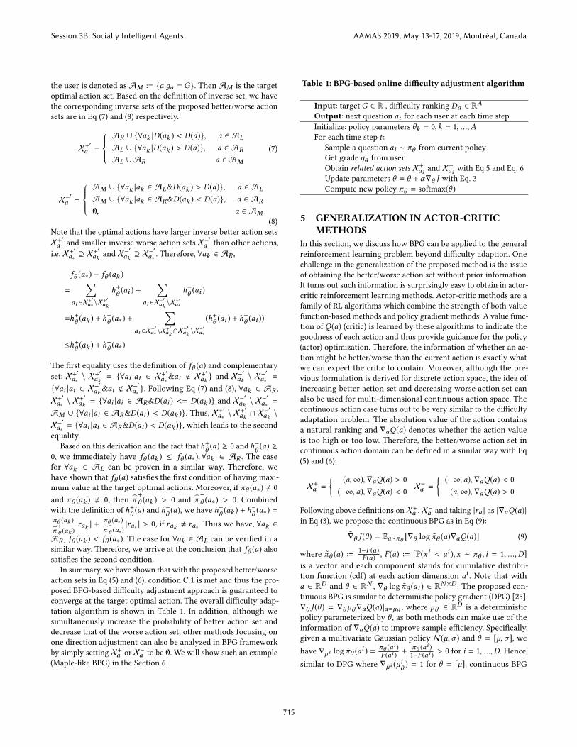
Table 1: BPG-based online difficulty adjustment algorithm

Input: target G ∈ R , difficulty ranking Da ∈ RA

Output: next question ai for each user at each time step

Initialize: policy parameters θk = 0,k = 1, ...,AFor each time step t :

Sample a question ai ∼ πθ from current policy

Get grade дa from user

Obtain related action sets X+ai and X−ai with Eq.5 and Eq. 6

Update parameters θ = θ + α∇θ J with Eq. 3

Compute new policy πθ = softmax(θ )

5 GENERALIZATION IN ACTOR-CRITICMETHODS

In this section, we discuss how BPG can be applied to the general

reinforcement learning problem beyond difficulty adaption. One

challenge in the generalization of the proposed method is the issue

of obtaining the better/worse action set without prior information.

It turns out such information is surprisingly easy to obtain in actor-

critic reinforcement learning methods. Actor-critic methods are a

family of RL algorithms which combine the strength of both value

function-based methods and policy gradient methods. A value func-

tion of Q(a) (critic) is learned by these algorithms to indicate the

goodness of each action and thus provide guidance for the policy

(actor) optimization. Therefore, the information of whether an ac-

tion might be better/worse than the current action is exactly what

we can expect the critic to contain. Moreover, although the pre-

vious formulation is derived for discrete action space, the idea of

increasing better action set and decreasing worse action set can

also be used for multi-dimensional continuous action space. The

continuous action case turns out to be very similar to the difficulty

adaptation problem. The absolution value of the action contains

a natural ranking and ∇aQ(a) denotes whether the action value

is too high or too low. Therefore, the better/worse action set in

continuous action domain can be defined in a similar way with Eq

(5) and (6):

X+a =

{(a,∞),∇aQ(a) > 0

(−∞,a),∇aQ(a) < 0

X−a =

{(−∞,a),∇aQ(a) < 0

(a,∞),∇aQ(a) > 0

Following above definitions on X+a , X−a and taking |ra | as |∇aQ(a)|

in Eq (3), we propose the continuous BPG as in Eq (9):

˜∇θ J (θ ) = Ea∼πθ [∇θ log πθ (a)∇aQ(a)] (9)

where πθ (a) :=1−F (a)F (a) , F (a) := [P(x i < ai ), x ∼ πθ , i = 1, ...,D]

is a vector and each component stands for cumulative distribu-

tion function (cdf) at each action dimension ai . Note that with

a ∈ RD and θ ∈ RN , ∇θ log πθ (ai ) ∈ RN×D

. The proposed con-

tinuous BPG is similar to deterministic policy gradient (DPG) [25]:

∇θ J (θ ) = ∇θ µθ∇aQ(a)|a=µθ , where µθ ∈ RD is a deterministic

policy parameterized by θ , as both methods can make use of the

information of ∇aQ(a) to improve sample efficiency. Specifically,

given a multivariate Gaussian policy N(µ,σ ) and θ = [µ,σ ], we

have ∇µ i log πθ (ai ) =

πθ (ai )F (ai ) +

πθ (ai )1−F (ai ) > 0 for i = 1, ...,D. Hence,

similar to DPG where ∇µ i (µiθ ) = 1 for θ = [µ], continuous BPG


715

also moves the policy in the direction of the gradient of Q and

converges at the places of ∇aQ(a) = 0. However, one common

limitation for continuous BPG and DPG is the local optimal issue

in the case of a non-convex Q function (e.g. neural network), due

to the dependence on ∇aQ(a). DPG is a deterministic policy and

only focuses on the area of a = µθ . Continuous BPG, on the other

hand, is stochastic and can incorporate the ∇aQ(a) information

even when a , µθ . Thus, continuous BPG might have the potential

to alleviate this local optimal problem, given that it can make use

a wider range of ∇aQ(a). A more rigorous convergence analysis

and detailed comparison between continuous BPG and DPG will

be conducted in the future work.

In practice, the critic function Q(a) is usually obtained using a

function approximator Qw (a). Generally, this replacement could

affect the gradient direction. However, similar to traditional sto-

chastic and deterministic policy gradient [25, 27], we give a family

of compatible function approximatorQw (a) for bootstrapped policygradient in Theorem 5.1 such that substituting Qw (a) into Eq (9)

will not affect the gradient.

Theorem 5.1. (Compatible function approximation) A functionapproximatorQw (a) is compatible with a bootstrapped policy ˜∇θ J (θ ) =Eai∼πθ [∇θ log πθ (ai )∇aQ

w (a)|ai ], if

(1) ∇aQw (a)|ai = ∇θ log πθ (ai )

Tw(2) w minimizes the mean-squared error, i.e. minw MSE(θ,w) =

E[ϵ(θ ,w)T ϵ(θ ,w)], where ϵ(θ ,w) = ∇aQw (a)|ai −∇aQ(a)|ai

Proof. Ifw minimizes the MSE then the gradient of ϵ2 w.r.twmust be zero.We then use the fact that, by condition (1),∇wϵ(θ,w) =

∇θ log πθ (ai ),

0 = ∇wMSE(θ ,w)

= E[∇θ log πθ (ai )ϵ(θ ,w)]

= E[∇θ log πθ (ai )(∇aQw (a)|ai − ∇aQ(a)|ai )]

(10)

Thus, E[∇θ log πθ (ai )∇aQw (a)|ai ] = E[∇θ log πθ (ai )∇aQ(a)|ai ]

�

For any stochastic policy πθ (a), there always exists a compatible

function approximator of the form Qw (a) = ϕ(a)Tw with action

features ϕ(a) := ∇θ log πθ (a)aTand parameters w . Although a

linear approximator is not effective for predicting action values

globally, it serves as a useful local critic to guide the parameter

update direction [25]. Regarding the condition (2), in theory, we

need to minimize the mean square error between the gradient of

Q(a) andQw (a). Since the true gradient∇aQ(a) is difficult to obtain,

in practice the parameter w is learned using the standard policy

evaluation method, like Sarsa or Q-learning. The detail discussion

regarding this issue can be found in [25]. In the experiment section,

we provide a concrete example of how to apply the bootstrapped

policy gradient for continuous-armed bandit.

6 EXPERIMENTS6.1 Difficulty Adaptation

6.1.1 Baseline Approaches. We compared our approach (BPG)

with five other methods:

(1) Random method: it always randomly selects questions

(2) Bisection method: a deterministic approach which repeatedly

bisects the difficulty interval and then selects a subinter-

val which may contain the ideal difficulty level for further

processing

(3) Policy gradient (PG): it updates policy based on Eq (2)

(4) Maple method: it heuristically increases the softmax weights

of harder questions when a task is too easy for this user ( i.e.

w = α1eдa−Gw,дa > G), and decreases the softmax weights

of harder questions otherwise (i.e.w = α2eдa−Gw,дa ≤ G)

[22] with α1 and α2 as parameters.

(5) Maple-like BPG (BPG_mpl)3: it uses the bootstrapped policy

gradient in Eq (3), but the better/worse action sets defined

following the rules used in Maple. Specifically, when the

question is too easy, the harder questions are considered

as the better action, i.e. ∀ai ∈ AL , X+ai := {∀ak |D(ak ) >

D(ai )},X−ai = ∅; otherwise, harder questions are regarded as

worse actions, i.e. ∀ai < AL ,X+ai := ∅,X−

ai := {∀ak |D(ak ) >D(ai )}.

A parameter sweep on step size is performed for all the ap-

proaches.

6.1.2 Dataset. The data is generated following a similar manner

in [5, 22]. The user performance is measured by grade д, whichis positively related to the probability of a user answering a task

correctly. Given a target grade value G, which indicates the best

user experience, the goal of the difficulty adjustment algorithm

is to select the questions to keep the user’s performance at the

target grade as close as possible. Each user’ ability is modeled by a

competence level sl . Each question is modeled by a difficulty level

ql . Given a pair of difficulty level and competence level, the grade

the user may receive after answering this question is computed

based on Item Response Theory [9]: д = β 1

1+eγ (ql−sl )+ (1− β)ε . We

set parameters γ = 1 and β = 0.1. Note that β controls the amount

of random noise ε ∼ U[0, 1) in the reward. In this setting, when the

question difficulty ql matches exactly with user ability sl , the gradeis 0.5 and thus the target grade G is set to be 0.5 in the experiment.

Two kinds of distributions are considered while generating the user

competency levels sl and question difficulty levels ql : the uniformdistribution U{1, 200} and Gaussian distribution N(100, 20). We

consider 500 users interact with the agent and each completes

50 questions. There are 1000 possible question for selection (i.e.

T = 50,A = 1000).

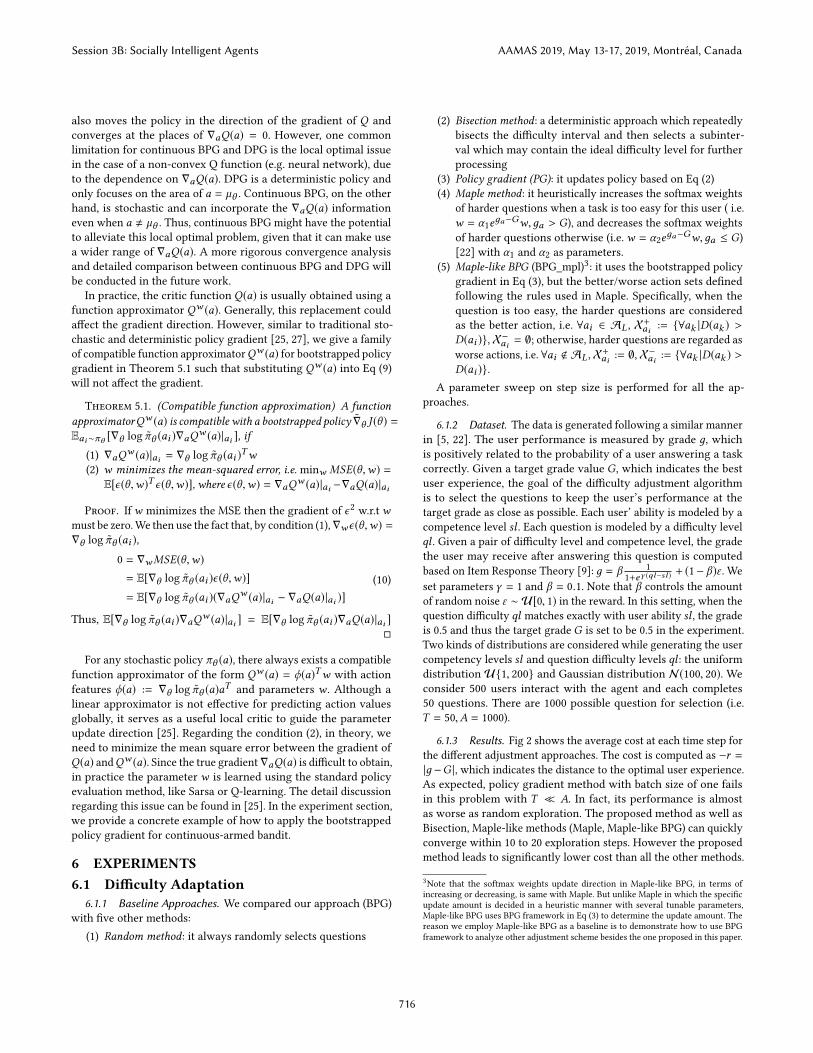
6.1.3 Results. Fig 2 shows the average cost at each time step for

the different adjustment approaches. The cost is computed as −r =|д −G |, which indicates the distance to the optimal user experience.

As expected, policy gradient method with batch size of one fails

in this problem with T ≪ A. In fact, its performance is almost

as worse as random exploration. The proposed method as well as

Bisection, Maple-like methods (Maple, Maple-like BPG) can quickly

converge within 10 to 20 exploration steps. However the proposed

method leads to significantly lower cost than all the other methods.

3Note that the softmax weights update direction in Maple-like BPG, in terms of

increasing or decreasing, is same with Maple. But unlike Maple in which the specific

update amount is decided in a heuristic manner with several tunable parameters,

Maple-like BPG uses BPG framework in Eq (3) to determine the update amount. The

reason we employ Maple-like BPG as a baseline is to demonstrate how to use BPG

framework to analyze other adjustment scheme besides the one proposed in this paper.


716

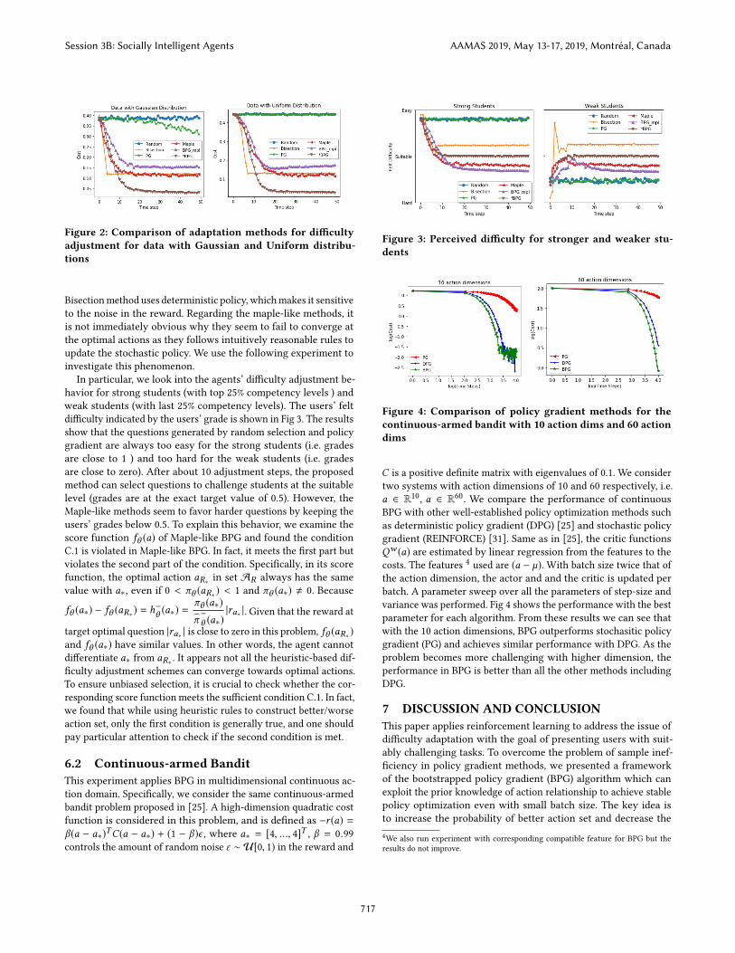
Figure 2: Comparison of adaptation methods for difficultyadjustment for data with Gaussian and Uniform distribu-tions

Bisectionmethod uses deterministic policy, whichmakes it sensitive

to the noise in the reward. Regarding the maple-like methods, it

is not immediately obvious why they seem to fail to converge at

the optimal actions as they follows intuitively reasonable rules to

update the stochastic policy. We use the following experiment to

investigate this phenomenon.

In particular, we look into the agents’ difficulty adjustment be-

havior for strong students (with top 25% competency levels ) and

weak students (with last 25% competency levels). The users’ felt

difficulty indicated by the users’ grade is shown in Fig 3. The results

show that the questions generated by random selection and policy

gradient are always too easy for the strong students (i.e. grades

are close to 1 ) and too hard for the weak students (i.e. grades

are close to zero). After about 10 adjustment steps, the proposed

method can select questions to challenge students at the suitable

level (grades are at the exact target value of 0.5). However, the

Maple-like methods seem to favor harder questions by keeping the

users’ grades below 0.5. To explain this behavior, we examine the

score function fθ (a) of Maple-like BPG and found the condition

C.1 is violated in Maple-like BPG. In fact, it meets the first part but

violates the second part of the condition. Specifically, in its score

function, the optimal action aR∗in set AR always has the same

value with a∗, even if 0 < πθ (aR∗) < 1 and πθ (a∗) , 0. Because

fθ (a∗) − fθ (aR∗) = h−θ (a∗) =

πθ (a∗)⌢π−

θ (a∗)|ra∗ |. Given that the reward at

target optimal question |ra∗ | is close to zero in this problem, fθ (aR∗)

and fθ (a∗) have similar values. In other words, the agent cannot

differentiate a∗ from aR∗. It appears not all the heuristic-based dif-

ficulty adjustment schemes can converge towards optimal actions.

To ensure unbiased selection, it is crucial to check whether the cor-

responding score function meets the sufficient condition C.1. In fact,

we found that while using heuristic rules to construct better/worse

action set, only the first condition is generally true, and one should

pay particular attention to check if the second condition is met.

6.2 Continuous-armed BanditThis experiment applies BPG in multidimensional continuous ac-

tion domain. Specifically, we consider the same continuous-armed

bandit problem proposed in [25]. A high-dimension quadratic cost

function is considered in this problem, and is defined as −r (a) =β(a − a∗)

TC(a − a∗) + (1 − β)ϵ , where a∗ = [4, ..., 4]T , β = 0.99

controls the amount of random noise ε ∼ U[0, 1) in the reward and

Figure 3: Perceived difficulty for stronger and weaker stu-dents

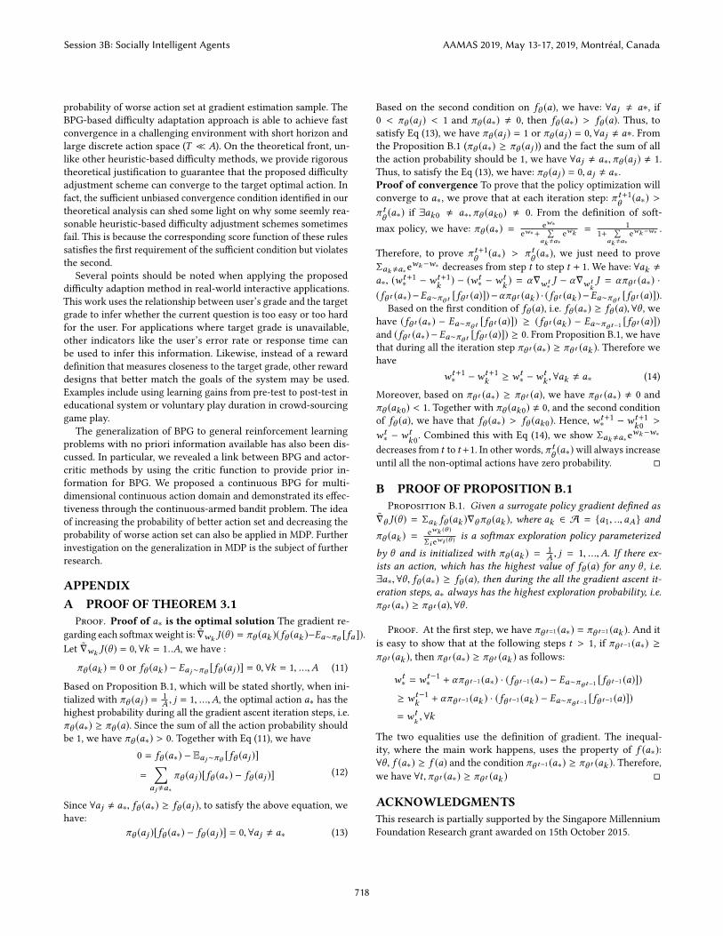
Figure 4: Comparison of policy gradient methods for thecontinuous-armed bandit with 10 action dims and 60 actiondims

C is a positive definite matrix with eigenvalues of 0.1. We consider

two systems with action dimensions of 10 and 60 respectively, i.e.

a ∈ R10, a ∈ R60. We compare the performance of continuous

BPG with other well-established policy optimization methods such

as deterministic policy gradient (DPG) [25] and stochastic policy

gradient (REINFORCE) [31]. Same as in [25], the critic functions

Qw (a) are estimated by linear regression from the features to the

costs. The features4used are (a − µ). With batch size twice that of

the action dimension, the actor and and the critic is updated per

batch. A parameter sweep over all the parameters of step-size and

variance was performed. Fig 4 shows the performance with the best

parameter for each algorithm. From these results we can see that

with the 10 action dimensions, BPG outperforms stochasitic policy

gradient (PG) and achieves similar performance with DPG. As the

problem becomes more challenging with higher dimension, the

performance in BPG is better than all the other methods including

DPG.

7 DISCUSSION AND CONCLUSIONThis paper applies reinforcement learning to address the issue of

difficulty adaptation with the goal of presenting users with suit-

ably challenging tasks. To overcome the problem of sample inef-

ficiency in policy gradient methods, we presented a framework

of the bootstrapped policy gradient (BPG) algorithm which can

exploit the prior knowledge of action relationship to achieve stable

policy optimization even with small batch size. The key idea is

to increase the probability of better action set and decrease the

4We also run experiment with corresponding compatible feature for BPG but the

results do not improve.


717

probability of worse action set at gradient estimation sample. The

BPG-based difficulty adaptation approach is able to achieve fast

convergence in a challenging environment with short horizon and

large discrete action space (T ≪ A). On the theoretical front, un-

like other heuristic-based difficulty methods, we provide rigorous

theoretical justification to guarantee that the proposed difficulty

adjustment scheme can converge to the target optimal action. In

fact, the sufficient unbiased convergence condition identified in our

theoretical analysis can shed some light on why some seemly rea-

sonable heuristic-based difficulty adjustment schemes sometimes

fail. This is because the corresponding score function of these rules

satisfies the first requirement of the sufficient condition but violates

the second.

Several points should be noted when applying the proposed

difficulty adaption method in real-world interactive applications.

This work uses the relationship between user’s grade and the target

grade to infer whether the current question is too easy or too hard

for the user. For applications where target grade is unavailable,

other indicators like the user’s error rate or response time can

be used to infer this information. Likewise, instead of a reward

definition that measures closeness to the target grade, other reward

designs that better match the goals of the system may be used.

Examples include using learning gains from pre-test to post-test in

educational system or voluntary play duration in crowd-sourcing

game play.

The generalization of BPG to general reinforcement learning

problems with no priori information available has also been dis-

cussed. In particular, we revealed a link between BPG and actor-

critic methods by using the critic function to provide prior in-

formation for BPG. We proposed a continuous BPG for multi-

dimensional continuous action domain and demonstrated its effec-

tiveness through the continuous-armed bandit problem. The idea

of increasing the probability of better action set and decreasing the

probability of worse action set can also be applied in MDP. Further

investigation on the generalization in MDP is the subject of further

research.

APPENDIXA PROOF OF THEOREM 3.1

Proof. Proof of a∗ is the optimal solution The gradient re-

garding each softmaxweight is:˜∇wk J (θ ) = πθ (ak )(fθ (ak )−Ea∼πθ [fa ]).

Let˜∇wk J (θ ) = 0,∀k = 1..A, we have :

πθ (ak ) = 0 or fθ (ak ) − Eaj∼πθ [fθ (aj )] = 0,∀k = 1, ...,A (11)

Based on Proposition B.1, which will be stated shortly, when ini-

tialized with πθ (aj ) =1

A , j = 1, ...,A, the optimal action a∗ has thehighest probability during all the gradient ascent iteration steps, i.e.

πθ (a∗) ≥ πθ (a). Since the sum of all the action probability should

be 1, we have πθ (a∗) > 0. Together with Eq (11), we have

0 = fθ (a∗) − Eaj∼πθ [fθ (aj )]

=∑aj,a∗

πθ (aj )[fθ (a∗) − fθ (aj )](12)

Since ∀aj , a∗, fθ (a∗) ≥ fθ (aj ), to satisfy the above equation, we

have:

πθ (aj )[fθ (a∗) − fθ (aj )] = 0,∀aj , a∗ (13)

Based on the second condition on fθ (a), we have: ∀aj , a∗, if0 < πθ (aj ) < 1 and πθ (a∗) , 0, then fθ (a∗) > fθ (a). Thus, tosatisfy Eq (13), we have πθ (aj ) = 1 or πθ (aj ) = 0,∀aj , a∗. Fromthe Proposition B.1 (πθ (a∗) ≥ πθ (aj )) and the fact the sum of all

the action probability should be 1, we have ∀aj , a∗, πθ (aj ) , 1.

Thus, to satisfy the Eq (13), we have: πθ (aj ) = 0,aj , a∗.Proof of convergence To prove that the policy optimization will

converge to a∗, we prove that at each iteration step: π t+1θ (a∗) >

π tθ (a∗) if ∃ak0 , a∗, πθ (ak0) , 0. From the definition of soft-

max policy, we have: πθ (a∗) =ew∗

ew∗+

∑ak ,a∗

ewk =

1

1+∑

ak ,a∗ewk −w∗ .

Therefore, to prove π t+1θ (a∗) > π tθ (a∗), we just need to prove

Σak,a∗ewk−w∗

decreases from step t to step t + 1. We have: ∀ak ,

a∗, (wt+1∗ − wt+1

k ) − (wt∗ − wt

k ) = α∇w t∗J − α∇w t

kJ = απθ t (a∗) ·

(fθ t (a∗)−Ea∼πθ t [fθ t (a)])−απθ t (ak ) · (fθ t (ak )−Ea∼πθ t [fθ t (a)]).Based on the first condition of fθ (a), i.e. fθ (a∗) ≥ fθ (a),∀θ , we

have (fθ t (a∗) − Ea∼πθ t [fθ t (a)]) ≥ (fθ t (ak ) − Ea∼πθ t−1 [fθ t (a)])and (fθ t (a∗) − Ea∼πθ t [fθ t (a)]) ≥ 0. From Proposition B.1, we have

that during all the iteration step πθ t (a∗) ≥ πθ t (ak ). Therefore wehave

wt+1∗ −wt+1

k ≥ wt∗ −wt

k ,∀ak , a∗ (14)

Moreover, based on πθ t (a∗) ≥ πθ t (a), we have πθ t (a∗) , 0 and

πθ (ak0) < 1. Together with πθ (ak0) , 0, and the second condition

of fθ (a), we have that fθ (a∗) > fθ (ak0). Hence, wt+1∗ − wt+1

k0 >

wt∗ − wt

k0. Combined this with Eq (14), we show Σak,a∗ewk−w∗

decreases from t to t+1. In other words, π tθ (a∗)will always increaseuntil all the non-optimal actions have zero probability. �

B PROOF OF PROPOSITION B.1Proposition B.1. Given a surrogate policy gradient defined as

˜∇θ J (θ ) = Σak fθ (ak )∇θπθ (ak ), where ak ∈ A = {a1, ..,aA} and

πθ (ak ) =ewk (θ )

Σi ewi (θ )is a softmax exploration policy parameterized

by θ and is initialized with πθ (ak ) =1

A , j = 1, ...,A. If there ex-ists an action, which has the highest value of fθ (a) for any θ , i.e.∃a∗,∀θ, fθ (a∗) ≥ fθ (a), then during the all the gradient ascent it-eration steps, a∗ always has the highest exploration probability, i.e.πθ t (a∗) ≥ πθ t (a),∀θ .

Proof. At the first step, we have πθ t=1 (a∗) = πθ t=1 (ak ). And it

is easy to show that at the following steps t > 1, if πθ t−1 (a∗) ≥

πθ t (ak ), then πθ t (a∗) ≥ πθ t (ak ) as follows:

wt∗ = w

t−1∗ + απθ t−1 (a∗) · (fθ t−1 (a∗) − Ea∼πθ t−1 [fθ t−1 (a)])

≥ wt−1k + απθ t−1 (ak ) · (fθ t−1 (ak ) − Ea∼πθ t−1 [fθ t−1 (a)])

= wtk,∀k

The two equalities use the definition of gradient. The inequal-

ity, where the main work happens, uses the property of f (a∗):∀θ , f (a∗) ≥ f (a) and the condition πθ t−1 (a∗) ≥ πθ t (ak ). Therefore,

we have ∀t, πθ t (a∗) ≥ πθ t (ak ) �

ACKNOWLEDGMENTSThis research is partially supported by the Singapore Millennium

Foundation Research grant awarded on 15th October 2015.


718

REFERENCES[1] Seth Chaiklin. 2003. The zone of proximal development in Vygotsky’s analysis

of learning and instruction. Vygotsky’s educational theory in cultural context 1(2003), 39–64.

[2] Olivier Chapelle and Lihong Li. 2011. An empirical evaluation of thompson

sampling. In Advances in neural information processing systems. 2249–2257.[3] Min Chi, Kurt VanLehn, Diane Litman, and Pamela Jordan. 2011. An evaluation

of pedagogical tutorial tactics for a natural language tutoring system: A rein-

forcement learning approach. International Journal of Artificial Intelligence inEducation 21, 1-2 (2011), 83–113.

[4] Kamil Ciosek and Shimon Whiteson. 2017. Expected policy gradients. arXivpreprint arXiv:1706.05374 (2017).

[5] Benjamin Clement, Didier Roy, Pierre-Yves Oudeyer, and Manuel Lopes. 2015.

Multi-Armed Bandits for Intelligent Tutoring Systems. Journal of EducationalData Mining 7, 2 (2015).

[6] Mihaly Csikszentmihalyi. 2014. Toward a psychology of optimal experience. In

Flow and the foundations of positive psychology. Springer, 209–226.[7] Ganesh Ghalme, Shweta Jain, Sujit Gujar, and Y Narahari. 2017. Thompson

Sampling Based Mechanisms for Stochastic Multi-Armed Bandit Problems. In

Proceedings of the 16th Conference on Autonomous Agents and MultiAgent Systems.International Foundation for Autonomous Agents and Multiagent Systems, 87–

95.

[8] Shixiang Gu, Timothy Lillicrap, Zoubin Ghahramani, Richard E Turner, and

Sergey Levine. 2016. Q-prop: Sample-efficient policy gradient with an off-policy

critic. arXiv preprint arXiv:1611.02247 (2016).

[9] Ronald K Hambleton, Hariharan Swaminathan, and H Jane Rogers. 1991. Funda-mentals of item response theory. Vol. 2. Sage.

[10] Andrew S Lan and Richard G Baraniuk. 2016. A Contextual Bandits Framework

for Personalized Learning Action Selection.. In EDM. 424–429.

[11] Hao Liu, Yihao Feng, Yi Mao, Dengyong Zhou, Jian Peng, and Qiang Liu. 2018.

Action-dependent control variates for policy optimization via stein identity.

(2018).

[12] Yun-En Liu, Travis Mandel, Emma Brunskill, and Zoran Popovic. 2014. Trading

Off Scientific Knowledge and User Learning with Multi-Armed Bandits.. In EDM.

161–168.

[13] Travis Mandel, Yun-En Liu, Sergey Levine, Emma Brunskill, and Zoran Popovic.

2014. Offline policy evaluation across representations with applications to educa-

tional games. In Proceedings of the 2014 international conference on Autonomousagents and multi-agent systems. International Foundation for Autonomous Agents

and Multiagent Systems, 1077–1084.

[14] Volodymyr Mnih, Adria Puigdomenech Badia, Mehdi Mirza, Alex Graves, Tim-

othy Lillicrap, Tim Harley, David Silver, and Koray Kavukcuoglu. 2016. Asyn-

chronous methods for deep reinforcement learning. In International conferenceon machine learning. 1928–1937.

[15] Volodymyr Mnih, Koray Kavukcuoglu, David Silver, Andrei A Rusu, Joel Veness,

Marc G Bellemare, Alex Graves, Martin Riedmiller, Andreas K Fidjeland, Georg

Ostrovski, et al. 2015. Human-level control through deep reinforcement learning.

Nature 518, 7540 (2015), 529.[16] Ian Osband, Charles Blundell, Alexander Pritzel, and Benjamin Van Roy. 2016.

Deep exploration via bootstrapped DQN. In Advances in neural informationprocessing systems. 4026–4034.

[17] Jan Papoušek and Radek Pelánek. 2015. Impact of adaptive educational sys-

tem behaviour on student motivation. In International Conference on ArtificialIntelligence in Education. Springer, 348–357.

[18] Jan Papoušek, Vít Stanislav, and Radek Pelánek. 2016. Impact of question difficulty

on engagement and learning. In International Conference on Intelligent TutoringSystems. Springer, 267–272.

[19] Tom Schaul, John Quan, Ioannis Antonoglou, and David Silver. 2015. Prioritized

experience replay. arXiv preprint arXiv:1511.05952 (2015).[20] John Schulman, Sergey Levine, Pieter Abbeel, Michael Jordan, and Philipp Moritz.

2015. Trust region policy optimization. In International Conference on MachineLearning. 1889–1897.

[21] John Schulman, Philipp Moritz, Sergey Levine, Michael Jordan, and Pieter Abbeel.

2015. High-dimensional continuous control using generalized advantage estima-

tion. arXiv preprint arXiv:1506.02438 (2015).[22] Avi Segal, Yossi Ben David, Joseph Jay Williams, Kobi Gal, and Yaar Shalom. 2018.

Combining Difficulty Ranking with Multi-Armed Bandits to Sequence Educa-

tional Content. In International Conference on Artificial Intelligence in Education.Springer, 317–321.

[23] Avi Segal, Kobi Gal, Ece Kamar, Eric Horvitz, and Grant Miller. 2018. Optimizing

Interventions via Offline Policy Evaluation: Studies in Citizen Science. (2018).

[24] Guy Shani and Bracha Shapira. 2014. Edurank: A collaborative filtering approach

to personalization in e-learning. Educational data mining (2014), 68–75.

[25] David Silver, Guy Lever, Nicolas Heess, Thomas Degris, Daan Wierstra, and

Martin Riedmiller. 2014. Deterministic policy gradient algorithms. In ICML.[26] Richard S Sutton and AndrewG Barto. 1998. Introduction to reinforcement learning.

Vol. 135. MIT press Cambridge.

[27] Richard S Sutton, David AMcAllester, Satinder P Singh, and YishayMansour. 2000.

Policy gradient methods for reinforcement learning with function approximation.

In Advances in neural information processing systems. 1057–1063.[28] Emanuel Todorov, Tom Erez, and Yuval Tassa. 2012. Mujoco: A physics engine

for model-based control. In Intelligent Robots and Systems (IROS), 2012 IEEE/RSJInternational Conference on. IEEE, 5026–5033.

[29] George Tucker, Surya Bhupatiraju, Shixiang Gu, Richard E Turner, Zoubin

Ghahramani, and Sergey Levine. 2018. The mirage of action-dependent baselines

in reinforcement learning. arXiv preprint arXiv:1802.10031 (2018).[30] Ziyu Wang, Tom Schaul, Matteo Hessel, Hado Van Hasselt, Marc Lanctot, and

Nando De Freitas. 2015. Dueling network architectures for deep reinforcement

learning. arXiv preprint arXiv:1511.06581 (2015).[31] Ronald J Williams. 1992. Simple statistical gradient-following algorithms for

connectionist reinforcement learning. Machine learning 8, 3-4 (1992), 229–256.

[32] Cathy Wu, Aravind Rajeswaran, Yan Duan, Vikash Kumar, Alexandre M Bayen,

Sham Kakade, Igor Mordatch, and Pieter Abbeel. 2018. Variance reduction

for policy gradient with action-dependent factorized baselines. arXiv preprintarXiv:1803.07246 (2018).


719

bootstrapped policy gradient for difficulty adaptation in

Documents