boundary variational inequality approach in the ... · georgian mathematical journal volume 8...
TRANSCRIPT

Georgian Mathematical JournalVolume 8 (2001), Number 3, 469–492
BOUNDARY VARIATIONAL INEQUALITY APPROACH INTHE ANISOTROPIC ELASTICITY FOR THE SIGNORINI
PROBLEM
A. GACHECHILADZE AND D. NATROSHVILI
Abstract. The purpose of the paper is reducing the three-dimensional Sig-norini problem to a variational inequality which occurs on the two-dimen-sional boundary of a domain occupied by an elastic anisotropic body. Theuniqueness and existence theorems for the solution of the boundary varia-tional inequality are proved and a boundary element procedure together withan abstract error estimate is described for the Galerkin numerical approxi-mation.
2000 Mathematics Subject Classification: 35J85, 74B05.Key words and phrases: Signorini problem, anisotropic elasticity, varia-tional inequalities.
1. Introduction
Signorini type problems in the elasticity theory are well studied (see [11], [12],[21], [7], [19], and the references therein). The main tool to investigate theseproblems is the theory of spatial variational inequalities. By this method theuniqueness and existence theorems are proved and the regularity properties ofsolutions are established in various functional spaces.
The purpose of the present paper is reducing of the three-dimensional Sig-norini problem to a variational inequality which occurs on the two-dimensionalboundary of a domain occupied by the elastic anisotropic body under consid-eration. We will show that the spatial variational inequality (SVI) is equivalentto the boundary variational inequality (BVI) obtained. The uniqueness and ex-istence theorems for the solution of BVI are proved, and a boundary elementprocedure together with an abstract error estimate is described for the Galerkinnumerical approximation.
A similar approach in the isotropic case is considered in [16], [17], [15], wherethe Signorini problem is reduced to a system consisting of a BVI and a boundarysingular integral equation (for related problems see also [9], [8] and the referencestherein).
2. Classical and Spatial Variational Inequality Formulations ofthe Signorini Problem
2.1. Let an elastic homogeneous anisotropic body in the natural configuration
ISSN 1072-947X / $8.00 / c© Heldermann Verlag www.heldermann.de
470 A. GACHECHILADZE AND D. NATROSHVILI
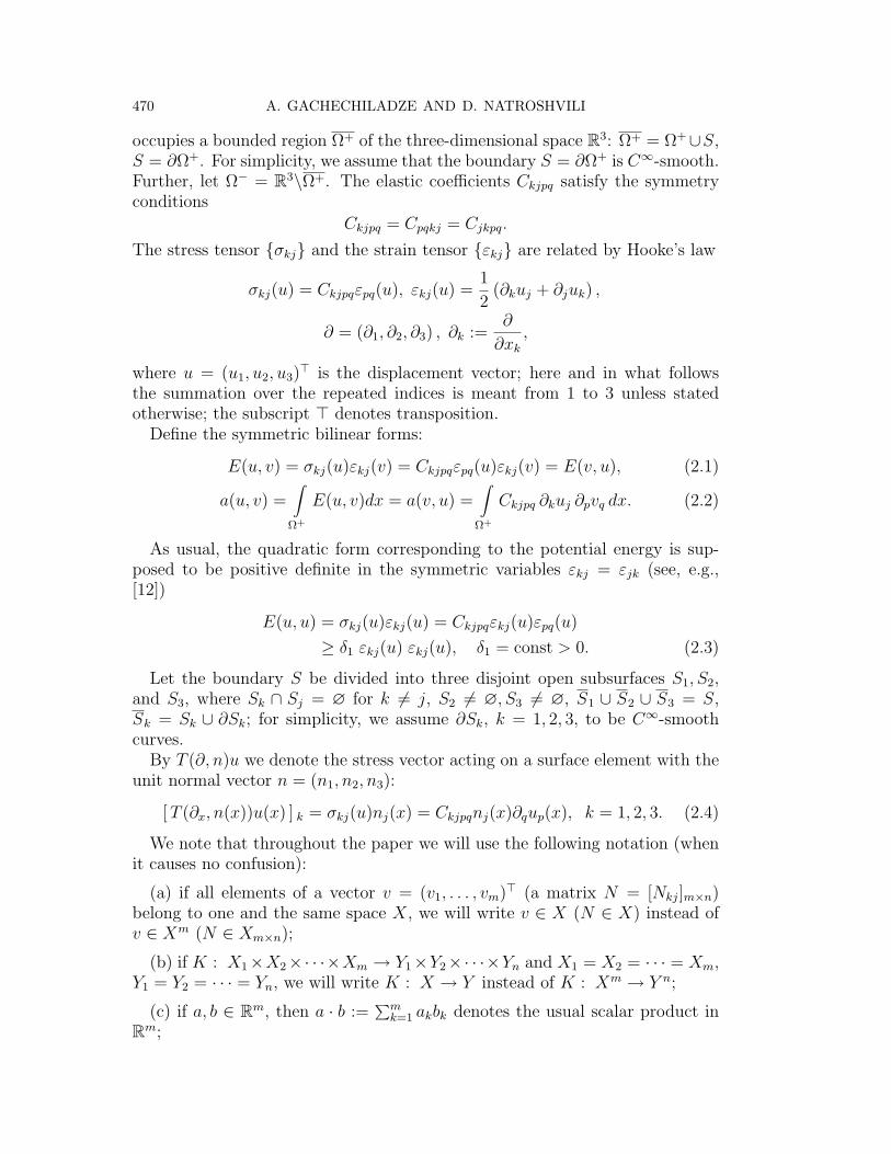
occupies a bounded region Ω+ of the three-dimensional space R3: Ω+ = Ω+∪S,S = ∂Ω+. For simplicity, we assume that the boundary S = ∂Ω+ is C∞-smooth.Further, let Ω− = R3\Ω+. The elastic coefficients Ckjpq satisfy the symmetryconditions
Ckjpq = Cpqkj = Cjkpq.
The stress tensor σkj and the strain tensor εkj are related by Hooke’s law
σkj(u) = Ckjpqεpq(u), εkj(u) =1
2(∂kuj + ∂juk) ,
∂ = (∂1, ∂2, ∂3) , ∂k :=∂
∂xk
,
where u = (u1, u2, u3)> is the displacement vector; here and in what follows
the summation over the repeated indices is meant from 1 to 3 unless statedotherwise; the subscript > denotes transposition.
Define the symmetric bilinear forms:
E(u, v) = σkj(u)εkj(v) = Ckjpqεpq(u)εkj(v) = E(v, u), (2.1)
a(u, v) =∫
Ω+
E(u, v)dx = a(v, u) =∫
Ω+
Ckjpq ∂kuj ∂pvq dx. (2.2)
As usual, the quadratic form corresponding to the potential energy is sup-posed to be positive definite in the symmetric variables εkj = εjk (see, e.g.,[12])
E(u, u) = σkj(u)εkj(u) = Ckjpqεkj(u)εpq(u)
≥ δ1 εkj(u) εkj(u), δ1 = const > 0. (2.3)
Let the boundary S be divided into three disjoint open subsurfaces S1, S2,and S3, where Sk ∩ Sj = ∅ for k 6= j, S2 6= ∅, S3 6= ∅, S1 ∪ S2 ∪ S3 = S,Sk = Sk ∪ ∂Sk; for simplicity, we assume ∂Sk, k = 1, 2, 3, to be C∞-smoothcurves.
By T (∂, n)u we denote the stress vector acting on a surface element with theunit normal vector n = (n1, n2, n3):
[ T (∂x, n(x))u(x) ] k = σkj(u)nj(x) = Ckjpqnj(x)∂qup(x), k = 1, 2, 3. (2.4)
We note that throughout the paper we will use the following notation (whenit causes no confusion):
(a) if all elements of a vector v = (v1, . . . , vm)> (a matrix N = [Nkj]m×n)belong to one and the same space X, we will write v ∈ X (N ∈ X) instead ofv ∈ Xm (N ∈ Xm×n);
(b) if K : X1×X2×· · ·×Xm → Y1×Y2×· · ·×Yn and X1 = X2 = · · · = Xm,Y1 = Y2 = · · · = Yn, we will write K : X → Y instead of K : Xm → Y n;
(c) if a, b ∈ Rm, then a · b :=∑m
k=1 akbk denotes the usual scalar product inRm;
BOUNDARY VARIATIONAL INEQUALITY APPROACH 471
(d) by ‖u; X‖ we denote the norm of the element u in the space X.
As usual, Hα(Ω+), Hαloc(Ω
−) and Hα(S) denote the Sobolev-Slobodetski(Bessel potential) spaces; here α is a real number (see, e.g., [22], [31], [32]).
By Hα(Sk) we denote the subspace of Hα(S):
Hα(Sk) = ω : ω ∈ Hα(S), supp ω ⊂ Sk,while Hα(Sk) denotes the space of restriction on Sk of functionals from Hα(S)
Hα(Sk) = rSkf : f ∈ Hα(S),
where rSkdenotes the restriction operator on Sk.
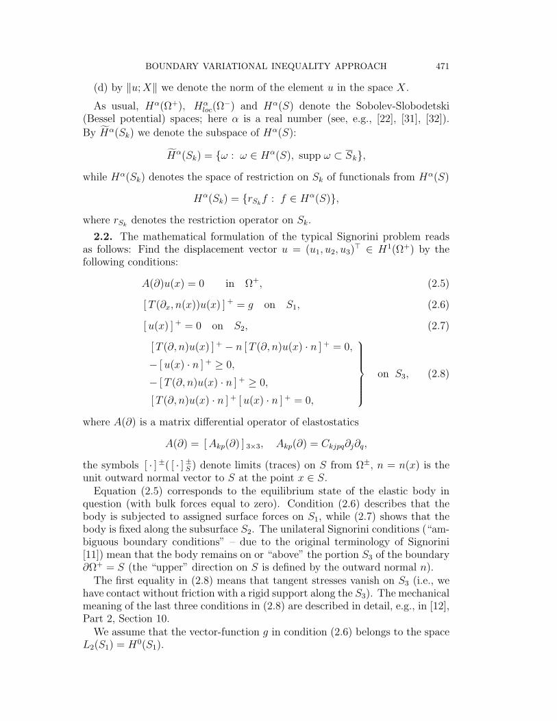
2.2. The mathematical formulation of the typical Signorini problem readsas follows: Find the displacement vector u = (u1, u2, u3)
> ∈ H1(Ω+) by thefollowing conditions:
A(∂)u(x) = 0 in Ω+, (2.5)
[ T (∂x, n(x))u(x) ] + = g on S1, (2.6)
[ u(x) ] + = 0 on S2, (2.7)
[ T (∂, n)u(x) ] + − n [ T (∂, n)u(x) · n ] + = 0,
− [ u(x) · n ] + ≥ 0,
− [ T (∂, n)u(x) · n ] + ≥ 0,
[ T (∂, n)u(x) · n ] + [ u(x) · n ] + = 0,
on S3, (2.8)
where A(∂) is a matrix differential operator of elastostatics
A(∂) = [ Akp(∂) ] 3×3, Akp(∂) = Ckjpq∂j∂q,
the symbols [ · ] ±( [ · ] ±S ) denote limits (traces) on S from Ω±, n = n(x) is theunit outward normal vector to S at the point x ∈ S.
Equation (2.5) corresponds to the equilibrium state of the elastic body inquestion (with bulk forces equal to zero). Condition (2.6) describes that thebody is subjected to assigned surface forces on S1, while (2.7) shows that thebody is fixed along the subsurface S2. The unilateral Signorini conditions (“am-biguous boundary conditions” – due to the original terminology of Signorini[11]) mean that the body remains on or “above” the portion S3 of the boundary∂Ω+ = S (the “upper” direction on S is defined by the outward normal n).
The first equality in (2.8) means that tangent stresses vanish on S3 (i.e., wehave contact without friction with a rigid support along the S3). The mechanicalmeaning of the last three conditions in (2.8) are described in detail, e.g., in [12],Part 2, Section 10.
We assume that the vector-function g in condition (2.6) belongs to the spaceL2(S1) = H0(S1).
472 A. GACHECHILADZE AND D. NATROSHVILI
Note that if u ∈ H1(Ω+) and A(∂)u ∈ L2(Ω+), then, in general, the limit
[ T (∂, n)u ] +S is defined as a functional of the class H− 1
2 (S) defined by the dualityrelation (see, e.g., [22]),
〈 [ T (∂, n)u(x) ] +S , [v]+S 〉S :=
∫
Ω+
A(∂)u · v dx +∫
Ω+
E(u, v) dx, (2.9)
where v = (v1, v2, v3)> ∈ H1(Ω+); here 〈·, ·〉S is the duality between the spaces
H12 (S) and H− 1
2 (S), which coincides with the usual [ L2(S) ] 3 scalar product forregular (in general, complex valued) vector-functions, i.e., if f, h ∈ [ L2(S) ] 3,then
〈f, h〉S =∫
S
fkhk dS =: (f, h)L2(S),
where the over-bar denotes complex conjugation.Equation (2.9) can be interpreted as a Green formula for the operator A(∂).Due to the regularity results obtained in [19] if, in addition, g = [G]+S1
, whereG ∈ H1(Ω+), then all conditions in (2.8) can be understood in the usual classicalsense (see also [12], Part 2, Section 10).
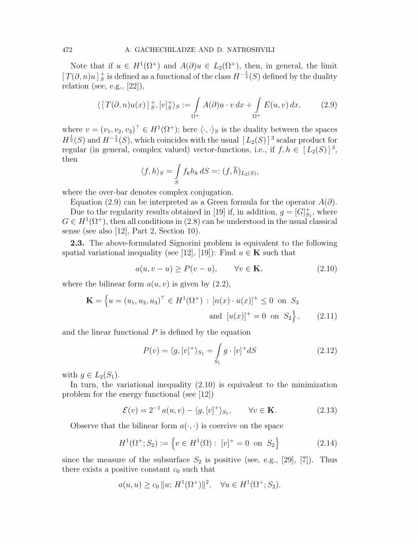
2.3. The above-formulated Signorini problem is equivalent to the followingspatial variational inequality (see [12], [19]): Find u ∈ K such that
a(u, v − u) ≥ P (v − u), ∀v ∈ K, (2.10)
where the bilinear form a(u, v) is given by (2.2),
K =u = (u1, u2, u3)
> ∈ H1(Ω+) : [n(x) · u(x)]+ ≤ 0 on S3
and [u(x)]+ = 0 on S2
, (2.11)
and the linear functional P is defined by the equation
P (v) = 〈g, [v]+〉S1 =∫
S1
g · [v]+dS (2.12)
with g ∈ L2(S1).In turn, the variational inequality (2.10) is equivalent to the minimization
problem for the energy functional (see [12])
E(v) = 2−1 a(u, v)− 〈g, [v]+〉S1 , ∀v ∈ K. (2.13)
Observe that the bilinear form a(·, ·) is coercive on the space
H1(Ω+; S2) :=v ∈ H1(Ω) : [v]+ = 0 on S2
(2.14)
since the measure of the subsurface S2 is positive (see, e.g., [29], [7]). Thusthere exists a positive constant c0 such that
a(u, u) ≥ c0 ‖u; H1(Ω+)‖2, ∀u ∈ H1(Ω+; S2).

BOUNDARY VARIATIONAL INEQUALITY APPROACH 473
Therefore the variational inequality (2.10) together with problem (2.5)–(2.8)and the minimization problem for functional (2.13) is uniquely solvable (see,e.g., [12], [7], [19], [13]).
In the subsequent sections, on the basis of the potential theory, we will equiv-alently reduce the spatial variational inequality (2.10) to a boundary variationalinequality.
First we expose the mapping and coercive properties of the integral (pseu-dodifferential) operators.
3. Properties of Boundary Integral (Pseudodifferential)Operators
3.1. Single- and double-layer potentials and their properties. LetΓ(·) be the fundamental matrix of the operator A(∂)
A(∂)Γ(x) = δ(x)I,
where δ(·) is the Dirac distribution and I = [δkj]3×3 is the unit matrix (δkj isthe Kronecker symbol). This matrix reads [Na1]
Γ(x) = F−1ξ→x [ A−1(−iξ) ] = − 1
8π|x|2π∫
0
A−1(aη)dϕ, (3.1)
where A−1(−iξ) is the matrix inverse to A(−iξ), ξ ∈ R3\0, x ∈ R3\0,a = [akj]3×3 is an orthogonal matrix with the property a>x = (0, 0, |x|)>, η =(cos ϕ, sin ϕ, 0)>; F−1
ξ→x denotes the generalized inverse Fourier transform.Further, let us introduce the single- and double-layer potentials
V (g)(x) =∫
S
Γ(x− y) g(y) dSy, (3.2)
W (g)(x) =∫
S
[T (∂y, n(y))Γ(x− y)]> g(y) dSy, (3.3)
where g = (g1, g2, g3)> is a density vector and x ∈ R3\ S.
The properties of these potentials and the corresponding boundary integral(pseudodifferential) operators in the Holder (Ck+α), Bessel potential (Hs
p) andBesov (Bs
p,q) spaces are studied in [20], [25], [2], [26], [27], [5], [6], [28] (seealso [18], [3], [24], where the coerciveness of boundary operators and Lipschitzdomains are considered).
In the sequel we need some results obtained in the above-cited papers andwe recall them here for convenience.
Theorem 3.1 ([25], [2], [26]). Let k ≥ 0 be an integer and 0 < γ < 1. Thenthe operators
V : Ck+γ(S) → Ck+1+γ(Ω±),
W : Ck+γ(S) → Ck+γ(Ω±),(3.4)
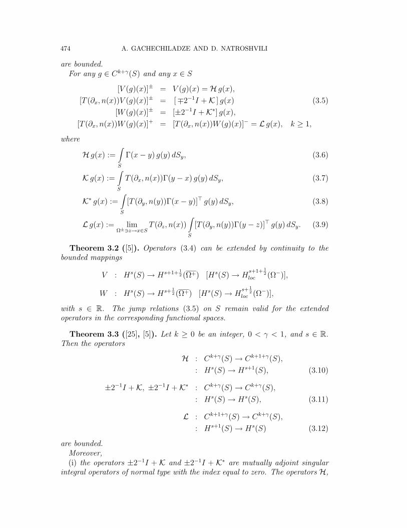
474 A. GACHECHILADZE AND D. NATROSHVILI
are bounded.For any g ∈ Ck+γ(S) and any x ∈ S
[V (g)(x)]± = V (g)(x) = H g(x),
[T (∂x, n(x))V (g)(x)]± = [∓2−1I +K ] g(x) (3.5)
[W (g)(x)]± = [±2−1I +K∗] g(x),
[T (∂x, n(x))W (g)(x)]+ = [T (∂x, n(x))W (g)(x)]− = L g(x), k ≥ 1,
where
H g(x) :=∫
S
Γ(x− y) g(y) dSy, (3.6)
K g(x) :=∫
S
T (∂x, n(x))Γ(y − x) g(y) dSy, (3.7)
K∗ g(x) :=∫
S
[T (∂y, n(y))Γ(x− y)]> g(y) dSy, (3.8)
L g(x) := limΩ±3z→x∈S
T (∂z, n(x))∫
S
[T (∂y, n(y))Γ(y − z)]> g(y) dSy. (3.9)
Theorem 3.2 ([5]). Operators (3.4) can be extended by continuity to thebounded mappings
V : Hs(S) → Hs+1+ 12 (Ω+) [Hs(S) → H
s+1+ 12
loc (Ω−)],
W : Hs(S) → Hs+ 12 (Ω+) [Hs(S) → H
s+ 12
loc (Ω−)],
with s ∈ R. The jump relations (3.5) on S remain valid for the extendedoperators in the corresponding functional spaces.
Theorem 3.3 ([25], [5]). Let k ≥ 0 be an integer, 0 < γ < 1, and s ∈ R.Then the operators
H : Ck+γ(S) → Ck+1+γ(S),
: Hs(S) → Hs+1(S), (3.10)
±2−1I +K, ±2−1I +K∗ : Ck+γ(S) → Ck+γ(S),
: Hs(S) → Hs(S), (3.11)
L : Ck+1+γ(S) → Ck+γ(S),
: Hs+1(S) → Hs(S) (3.12)
are bounded.Moreover,(i) the operators ±2−1I + K and ±2−1I + K∗ are mutually adjoint singular
integral operators of normal type with the index equal to zero. The operators H,
BOUNDARY VARIATIONAL INEQUALITY APPROACH 475
2−1I +K and 2−1I +K∗ are invertible. The inverse of HH−1 : Ck+1+γ(S) → Ck+γ(S) [Hs+1(S) → Hs(S)]
is a singular integro-differential operator;(ii) the L is a singular integro-differential operator and the following equalities
hold in appropriate functional spaces:
K∗H = HK, LK∗ = KL, HL = −4−1I + (K∗)2, LH = −4−1I +K2; (3.13)
(iii) The operators −H and L are self-adjoint and non-negative elliptic pseu-dodifferential operators with the index equal to zero:
〈−Hh, h〉S ≥ 0, 〈Lg, g〉S ≥ 0, (3.14)
∀h ∈ Cγ(S), ∀g ∈ C1+γ(S), [∀h ∈ H− 12 (S), ∀g ∈ H
12 (S) ] ,
with equality only for h = 0 and for
g = [a× x] + b, (3.15)
respectively; here a, b ∈ R3 are arbitrary constant vectors and [· × ·] denotes thecross product of two vectors;
(iv) a general solution of the homogeneous equations [−2−1I +K∗]g = 0 andLg = 0 is given by (3.15), i.e.,
kerL = ker(−2−1I +K∗
)and
dim kerL = dim cokerL = dim ker(−2−1I +K∗
)
= dim coker(−2−1I +K∗
)= 6.
Theorem 3.4 ([5], citeNa1). Let u be a solution of the homogeneous equa-tion A(D)u = 0 in Ω±. Then
W(
[ u ] ±)− V
([ Tu ] ±
)=
±u(x), x ∈ Ω±,
0, x ∈ Ω∓,
where either u ∈ Ck+γ(Ω±) with k ≥ 1, 0 < γ < 1, or u ∈ H1(Ω+) [ H1loc(Ω
−),u(x) → 0 as |x| → +∞ ] .
We also need some additional properties of the above-introduced operators,which will be proved below.
Theorem 3.5. Let f ∈ H12 (S) and h ∈ H− 1
2 (S) satisfy the condition(−2−1I +K∗
)f = Hh, i.e., h = H−1
(−2−1I +K∗
)f. (3.16)
Then there exists a unique vector-function u ∈ H1 (Ω+) such that
A (∂) u(x) = 0 in Ω+,
[ u ] + = f and [ Tu ] + = h on S = ∂Ω+.
476 A. GACHECHILADZE AND D. NATROSHVILI
Moreover,
Lf =(2−1I +K
)h, i.e., h =
(2−1I +K
)−1 Lf. (3.17)
Proof. We putu (x) = W (f)(x)− V (h) (x) , x ∈ Ω±.
Clearly, u ∈ H1(Ω+)∩H1loc(Ω
−) and A (∂) u(x) = 0 in Ω+. Due to Theorem 3.2and equality (3.16) we have
[ u ] − =(−2−1I +K∗
)f −Hh = 0.
Therefore, with the help of the uniqueness theorem for the exterior Dirichletboundary value problem (in Ω−) for the operator A(∂), we conclude that u(x) =0 in Ω−. Thus
W (g)(x)− V (h)(x) =
u(x) for x ∈ Ω+,
0 for x ∈ Ω−.
Whence, applying again Theorem3.2, we get
[ u ] + − [ u ] − = f and [ Tu ] + − [ Tu ] − = h on S,
i.e.,[ u ] + = f and [ Tu ] + = h.
The uniqueness of u can be easily shown by the uniqueness theorem for theDirichlet problem.
To complete the proof we note that (3.16) and Theorem3.3, (ii) imply
HLf =(2−1I +K∗
) (−2−1I +K∗
)f =
(2−1I +K∗
)Hh = H
(2−1I +K
)h,
from which (3.17) follows since H is an invertible operator.
Further, we discuss in detail the coercive properties of the bilinear forms in(3.14) and the operators related to them. Note that similar problems for theisotropic case and the Laplace equation are studied in [18], [3], [24], Ch.10, [4],Ch. XI, § 4 with the help of Korn’s inequalities. Here we treat the generalanisotropic case and prove the coerciveness of the corresponding operators bymeans of different arguments.
3.2. Coercive properties of the boundary bilinear forms. We startby the following simple lemma.
Lemma 3.6. Let 〈·, ·〉S be the bracket of duality (bilinear form) between thedual pair Hr(S) and H−r(S), ∀r ∈ R, and (·, ·)H−r(S) denote a scalar productin H−r(S).
There exists a linear bounded bijective operator
P2r : Hr(S) → H−r(S) (3.18)
and positive constants C1 and C2, such that
〈f, g〉S = (P2rf , g)H−r(S) , ∀f ∈ Hr(S), ∀g ∈ H−r(S), (3.19)

BOUNDARY VARIATIONAL INEQUALITY APPROACH 477
and
C1 ‖f ; Hr(S)‖ ≤ ‖P2rf ; H−r(S)‖ ≤ C2 ‖f ; Hr(S)‖, ∀f ∈ Hr(S). (3.20)
Moreover,
〈f, P2rf〉S ≥ 0, ∀f ∈ Hr(S), (3.21)
with the equality only for f = 0.
Proof. First we consider the case of real functions. Let f ∈ Hr(S). Then
|〈f, g〉S| ≤ C‖f ; Hr(S)‖ ‖g; H−r(S)‖, ∀g ∈ H−r(S),
where C is independent of f and g, i.e., 〈f, ·〉S is the linear bounded functional onH−r(S) and due to the Riesz theorem there exists a unique element F ∈ H−r(S)such that
〈f, g〉S = (F, g)H−r(S) , ∀g ∈ H−r(S). (3.22)
We put F = P2rf. It is evident that the mapping P2r : Hr(S) → H−r(S)is linear and injective. Now we show that it is surjective, i.e., for arbitraryF ∈ H−r(S) there exists unique f ∈ H−r(S) such that equality (3.22) holds.
Let Λr be an equivalent lifting (i.e., order reducing) pseudodifferential oper-ator of order −r (see, e.g., [22], [10], [14], [1]):
Λr : H0(S) → Hr(S).
This mapping is an isomorphism. Then the adjoint operator (with respect tothe duality bracket) Λ∗r is also an equivalent lifting operator
Λ∗r : [ Hr(S) ] ∗ → [ H0(S) ] ∗, i.e., Λ∗r : H−r(S) → H0(S).
Obviously, there exist positive constants a1, a2, b1, and b2 such that
a1 ‖f ; H0(S)‖ ≤ ‖Λrf ; Hr(S)‖ ≤ a2 ‖f ; H0(S)‖, ∀f ∈ H0(S),
b1 ‖g; H−r(S)‖ ≤ ‖Λ∗rg; H0(S)‖ ≤ b2 ‖g; H−r(S)‖, ∀g ∈ H−r(S).
Here aj and bj do not depend on f and g, respectively. Note that
B(f , g) := 〈ΛrΛ∗r f , g〉S
is a bilinear form on H−r(S)×H−r(S).Consider the equation
B(f , g) = (F, g)H−r(S) , ∀g ∈ H−r(S), (3.23)
where F ∈ H−r(S) is some given element and f ∈ H−r(S) is the sought forelement. Obviously, the linear functional in the right-hand side of (3.23) isbounded on H−r(S).
It is also evident that B(·, ·) is continuous:
|B(f , g)| = |〈ΛrΛ∗r f , g〉S| ≤ C ‖ΛrΛ
∗r f ; Hr(S)‖ ‖g; H−r(S)‖
≤ c a2 b2 ‖f ; H−r(S)‖ ‖g; H−r(S)‖.

478 A. GACHECHILADZE AND D. NATROSHVILI
Moreover, B(·, ·) is coercive:
B(f , f) = 〈ΛrΛ∗r f , f〉S = 〈Λ∗r f , Λ∗r f〉S =
(Λ∗r f , Λ∗r f
)H0(S)
= ‖Λ∗rf ; H0(S)‖2 ≥ b21 ‖f ; H−r(S)‖2.
Due to the Lax–Milgram theorem then there exists a unique solution f ∈H−r(S) of equation (3.23), i.e.,
〈ΛrΛ∗r f , g〉S = (F, g)H−r(S) , g ∈ H−r(S),
which proves the surjectivity of the operator P2r since ΛrΛ∗r f ∈ H−r(S). Thus
mapping (3.18) is bijective. Inequality (3.20) then follows from the Banachtheorem on inverse operators.
Now let f = f1 + if2 and g = g1 + ig2, where fj ∈ Hr(S) and gj ∈ H−r(S)are real functions.
Due to the results just proven we have
〈f, g〉S = 〈f1 + if2, g1 − ig2〉S = 〈f1, g1〉S + i〈f2, g1〉S − i〈f1, g2〉S−i2〈f2, g2〉S = (P2rf1, g1)H−r(S) + i (P2rf2, g1)H−r(S)
−i (P2rf1, g2)H−r(S) − i2 (P2rf2, g2)H−r(S) = (P2rf, g)H−r(S) ,
whence (3.20) and (3.21) follow.
Lemma 3.7. There exists a positive constant C3 such that
〈−Hϕ, ϕ〉S ≥ C3 ‖ϕ; H− 12 (S)‖2, ∀ϕ ∈ H− 1
2 (S).
Proof. Due to Lemma 3.6
〈−Hϕ, ϕ〉S = (−P1Hϕ, ϕ)H− 1
2 (S), ∀ϕ ∈ H− 1
2 (S).
Moreover, the mapping
−P1H : H− 12 (S) → H− 1
2 (S)
is an isomorphism and
(−P1Hϕ, ϕ)H− 1
2 (S)= 〈−Hϕ, ϕ〉S ≥ 0
for an arbitrary (complex-valued) function ϕ ∈ H− 12 (S). Evidently, −P1H is a
self-adjoint positive operator (see, e.g., [30], Theorem 12.32).By the square root theorem (see, e.g., [30], Theorem 12.33, [23], Ch.7, §3,
Theorem 2) we conclude that there exists a unique positive linear boundedbijective operator
Q : H− 12 (S) → H− 1
2 (S)
such that Q2 = −P1H. Consequently, Q is self-adjoint and invertible, and
e1 ‖ϕ; H− 12 (S)‖ ≤ ‖Qϕ; H− 1
2 (S)‖ ≤ e2 ‖ϕ; H− 12 (S)‖

BOUNDARY VARIATIONAL INEQUALITY APPROACH 479
with some positive constants e1 and e2. Therefore
〈−Hϕ, ϕ〉S = (−P1Hϕ, ϕ)H− 1
2 (S)
=(Q2ϕ, ϕ
)H− 1
2 (S)= ‖Qϕ; H− 1
2 (S)‖2 ≥ e21 ‖ϕ; H− 1
2 (S)‖2,
which completes the proof.
We denote by X(Ω+) the space of rigid displacements in Ω+, and by X(S) =X(∂Ω+) the space of their restrictions on S = ∂Ω+ (see (3.15)). Note thatdimX(Ω+) =dimX(S) = 6. Let Ψ(S) = χj6
j=1 be the orthonormal (in the
H0(S)-sense) basis in X(S):(χj, χk
)H0(S)
= 〈χj, χk〉S = δkj,
where δkj is Kronecker’s symbol. Clearly, the system χj6j=1 can be obtained
by the orthonormalization (in the H0(S)-sense) procedure of the following basisof X(S):
ν(1) = (1, 0, 0), ν(2) = (0, 1, 0), ν(3) = (0, 0, 1),
ν(4) = (x3, 0,−x1), ν(5) = (−x2, x3, 0), ν(6) = (0,−x3, x2).
Further, let r ∈ R and
Hr∗(S) := ϕ : ϕ ∈ Hr(S), 〈ϕ, χj〉S = 0, j = 1, 6. (3.24)
It is evident that Hr∗(S) is a Hilbert space with the scalar product induced by
(·, ·)Hr(S).
Lemma 3.8. L(H12 (S)) = H
− 12∗ (S), where the operator L is given by (3.9).
Proof. The Green identity∫
Ω+
[ Au · v − u · Av ] dx =∫
S
[ Tu ] + · [ v ] + − [ u ] + · [ Tv ] +
dS
with u = W (ϕ) and ∀v ∈ X(Ω+) yields∫
S
Lϕ · χjdS = 〈Lϕ, χj〉S = 0, ∀ϕ ∈ H12 (S), j = 1, 6.
Therefore
L : H12 (S) → H
− 12∗ (S), i.e., L(H
12 (S)) ⊂ H
− 12∗ (S).
On the other hand, the equation
Lϕ = f, f ∈ H− 1
2∗ (S), (3.25)
is solvable, and a solution ϕ ∈ H12 (S) can be represented in the form ([25], [5])
ϕ = ϕ0 +6∑
j=1
cjχj, ϕ0 ∈ H
12 (S),

480 A. GACHECHILADZE AND D. NATROSHVILI
where ϕ0 is some particular solution of the above non-homogeneous equation
and cj are arbitrary constants. In addition, if we require that ϕ ∈ H12∗ (S), then
(3.25) is uniquely solvable and the solution reads
ϕ = ϕ0 −6∑
j=1
〈ϕ0, χj〉S χj. (3.26)
It can be easily shown that the right-hand side in (3.26) does not depend on thechoice of the particular solution ϕ0 since the homogeneous version of equation
(3.25) (with f = 0) possesses only the trivial solution in the space H12∗ (S).
Corollary 3.9. The operator
L : H12∗ (S) → H
− 12∗ (S)
is an isomorphism, and the inequality
c∗1 ‖ϕ; H12 (S)‖ ≤ ‖Lϕ; H− 1
2 (S)‖ ≤ c∗2 ‖ϕ; H12 (S)‖, (3.27)
holds for all ϕ ∈ H12∗ (S) with some positive constants c∗1 and c∗2 independent
of ϕ.
Lemma 3.10. There exists a positive constant c∗3 such that
〈Lϕ, ϕ〉S ≥ c∗3 ‖ϕ; H12 (S)‖2, ∀ϕ ∈ H
12∗ (S).
Proof. Let
Lϕ := Lϕ +6∑
j=1
〈ϕ, χj〉Sχj.
Note that Lϕ = Lϕ if and only if ϕ ∈ H12∗ (S).
Evidently,
〈Lϕ, ϕ〉S = 〈Lϕ, ϕ〉S +6∑
j=1
|〈ϕ, χj〉S|2, ∀ϕ ∈ H12 (S),
and 〈Lϕ, ϕ〉S = 0 implies ϕ = 0, due to Theorem 3.3, (iii) and (iv). This alsoshows that the homogeneous equation
Lϕ = 0, ϕ ∈ H12 (S),
possesses only the trivial solution, and since Ind L = IndL = 0, we concludethat the mapping
L : H12 (S) → H− 1
2 (S)
is an isomorphism.Let Λ 1
2be an equivalent lifting operator
Λ 12
: H0(S) → H12 (S),
BOUNDARY VARIATIONAL INEQUALITY APPROACH 481
and construct the operator Λ∗12
LΛ 12, where Λ∗1
2
is the operator adjoint to Λ 12
with
respect to the duality bracket. Therefore the isomorphism Λ∗12
: H− 12 (S) →
H0(S) is also an equivalent lifting operator.It is obvious that the mapping
Λ∗12
LΛ 12
: H0(S) → H0(S) (3.28)
is an isomorphism. Moreover,
〈Λ∗12
LΛ 12ϕ, ϕ〉S = 〈LΛ 1
2ϕ, Λ 1
2ϕ〉S ≥ 0, ∀ϕ ∈ L2(S) = H0(S),
with equality only for ϕ = 0. Thus (3.28) defines a positive invertible operator.Further, due to the square root theorem, there exists a positive (self-adjoint)
invertible operator Q : H0(S) → H0(S) such that
Λ∗12
LΛ 12
= Q2.
Therefore, with the help of the self-adjointness of the operator Q and invokingthe Banach theorem on inverse operator, we get
〈Λ∗12
LΛ 12ϕ, ϕ〉S = 〈Q2ϕ, ϕ〉S =
(Q2ϕ, ϕ
)H0(S)
= ‖Qϕ; H0(S)‖2 ≥ c4‖ϕ; H0(S)‖2, ∀ϕ ∈ H0(S). (3.29)
Note that for arbitrary ψ ∈ H12 (S) there exists unique ϕ ∈ H0(S) such that
Λ 12ϕ = ψ, i.e., ψ = Λ−1
12
ϕ and ‖ϕ; H0(S)‖ ≥ c5‖ψ; H12 (S)‖, where c5 is a positive
constant independent of ϕ and ψ. Consequently, by virtue of (3.29) we derive
〈Lψ, ψ〉S = 〈LΛ 12ϕ, Λ 1
2ϕ〉S = 〈Λ∗1
2
LΛ 12ϕ, ϕ〉S
≥ c4 ‖ϕ; H0(S)‖2 ≥ c4c25 ‖ψ; H
12 (S)‖2,
which completes the proof since Lψ = Lψ, ∀ψ ∈ H12∗ (S).
Below we need some mapping and coercive properties of the operator
M := L −(−2−1I +K
)H−1
(−2−1I +K∗
). (3.30)
Applying equalities (3.13) we easily transform (3.30) to obtain
M = H−1(−2−1I +K∗
)=
(−2−1I +K
)H−1. (3.31)
Corollary 3.11. The operator
M : H12 (S) → H− 1
2 (S)
is a bounded, positive, formally self-adjoint (with respect to the duality bracket),elliptic pseudodifferential operator of order 1, and
kerM = kerL = ker(−2−1I +K∗
), IndM = 0.

482 A. GACHECHILADZE AND D. NATROSHVILI
Moreover,
M(H
12 (S)
)= H
− 12∗ (S).
The mapping
M : H12∗ (S) → H
− 12∗ (S)
is an isomorphism, and the inequalities
c′1 ‖ϕ; H12 (S)‖ ≤ ‖Mϕ; H− 1
2 (S)‖ ≤ c′2 ‖ϕ; H12 (S)‖, ∀ϕ ∈ H
12∗ (S),
〈Mϕ, ϕ〉S ≥ c′3 ‖ϕ; H12 (S)‖2, ∀ϕ ∈ H
12∗ (S),
hold with some positive constants c′1, c′2, and c′3 independent of ϕ.
Proof. It is a ready consequence of (3.30), (3.31), Theorem 3.3, Corollary 3.9,and Lemma 3.10.
4. Reduction to BVI. Existence and Uniqueness Results
Let u ∈ K be the unique solution of the SVI (2.10). Due to Theorems 3.4and 3.1 we have the following Steklov-Poincare relations connecting the Dirichletand Neumann boundary data on S = ∂Ω+ of the vector u:
L[u]+ =(2−1I +K
)[Tu]+,
(−2−1I +K∗
)[u]+ = H[Tu]+. (4.1)
These equalities imply
[Tu]+ = L[u]+ −(−2−1I +K
)[Tu]+
= L[u]+ −(−2−1I +K
)H−1
(−2−1I +K∗
)[u]+ = M[u]+, (4.2)
where M is defined by (3.30).The Green formula (2.9) with the vector u and arbitrary v ∈ H1(Ω+) can be
rewritten as∫
Ω+
E(u, v)dx = 〈 [ T (∂, n)u(x) ] +, [v]+〉S = 〈M[u]+, [v]+〉S, (4.3)
whence by virtue of (2.2)
a(u, v) = 〈M[u]+, [v]+〉S. (4.4)
Substituting (4.4) into (2.10) leads to the BVI: Find ϕ ∈ K(S) such that
〈Mϕ, ψ − ϕ〉S ≥∫
S1
g · (ψ − ϕ)dS, ∀ψ ∈ K(S), (4.5)
where, in our case, g ∈ L2(S1) is a given function (see(2.6)),
ϕ = [u]+, ψ = [v]+, (4.6)
K(S) :=f : f ∈ H
12 (S), n · f ≤ 0 on S3, f = 0 on S2
. (4.7)

BOUNDARY VARIATIONAL INEQUALITY APPROACH 483
Obviously, the closed convex cone K(S) coincides with the space of traces (onS) of functions from K (see (2.11)).
In what follows we show that the BVI (4.5) is equivalent to the SVI (2.10)in the following sense. If u is a solution of the SVI (2.10), then [u]+ = ϕ solvesthe BVI (4.5) which has just been proved.
Vice versa, if ϕ is a solution of the BVI (4.5), then the vector-function
u(x) = W (ϕ) (x)− V (h) (x), x ∈ Ω+, (4.8)
where (see (3.31))
h = H−1(−2−1I +K∗
)ϕ =
(−2−1I +K
)H−1ϕ = Mϕ (4.9)
solves the SVI (2.10). To prove this, we show that the vector-function (4.8)
meets conditions (2.5)–(2.8). Since ϕ ∈ H12 (S) and h ∈ H− 1
2 (S), it is evidentthat u ∈ H1(Ω+) by Theorem 3.2 and A(∂)u = 0 in Ω+. In accord with Theorem3.5 (see the proof of Theorem 3.5) we have ϕ = [u]+S and h = [Tu]+S = Mϕ.
Obviously, condition (2.7) holds since ϕ ∈ K.
If in (4.5) we put ψ = ϕ ± ψ ∈ K, where ψ ∈ H12 (S1), we arrive at the
equation
〈Mϕ, ψ〉S = 〈g, ψ〉S1 ∀ψ ∈ H12 (S1),
whence Mϕ = g on S1 follows, i.e., condition (2.6) holds as well.
Further, if in (4.5) we put ψ = ϕ± ω ∈ K, where ω ∈ H12 (S3) and ω · n = 0,
we get
〈Mϕ, ω〉S = 〈g, ω〉S3 , ∀ω ∈ H12 (S3), ω · n = 0,
which implies Mϕ − n(n · Mϕ) = 0 on S3. Thus, the first condition in (2.8)
holds automatically due to the inclusion ϕ ∈ K.Let us set ψ = ϕ−n ν, where n is the outward normal vector and ν ∈ H
12 (S3)
is a non-negative scalar function .From (4.5) then it follows
〈Mϕ,−nν〉S ≥ 0, i.e., 〈−n · Mϕ, ν〉S ≥ 0, ∀ν ∈ H12 (S3), ν ≥ 0.
This shows that the third inequality in (2.10) holds.Now, let h be a scalar function with the properties
0 ≤ h(x) ≤ 1, h ∈ C1(S), supp h ⊂ S3,
and put ψ = [1 + t h(x)]ϕ ∈ K with t ∈ (−1, 1). From inequality (4.5) then weget
〈Mϕ, h(x)ϕ〉S = 0,
which can be rewritten as
〈n · Mϕ, h(n · ϕ)〉S = 0 (4.10)
due to the equation Mϕ = n (n · Mϕ) on S3.Since h is an arbitrary function with the above-mentioned properties, from
(4.10) we conclude that the fourth condition in (2.8) also holds. The above
484 A. GACHECHILADZE AND D. NATROSHVILI
arguments prove that the vector u defined by (4.8) meets conditions (2.5)–(2.8)and therefore it solves the SVI (2.10).
Thus, there holds
Lemma 4.1. The SVI (2.10) is equivalent (in the above-mentioned sense)
to the following BVI: Find ϕ ∈ K such that
〈Mϕ, ψ − ϕ〉S ≥∫
S1
g · (ψ − ϕ)dS, ∀ψ ∈ K(S), (4.11)
with given g ∈ L2(S1).
From the existence and uniqueness theorems for the SVI (2.10) it followsthat BVI (4.11) is also uniquely solvable. Observe that to develop the Galerkinmethod for approximation of solutions by means of the boundary element pro-cedure and to obtain the corresponding abstract error estimate we need thecoercive property of the pseudodifferential operator M on the cone K(S). Thisproperty is also sine–qua–non to study the well–posedness of the BVI (4.11)independently (without invoking the mentioned SVI) on the basis of the theoryof abstract variational inequalities in Hilbert spaces.
Note that Corollary 3.11 proves the coercivity of the operatorM on the space
H12∗ (S). But, in general, the K(S) is not a subset of H
12∗ (S). However, there
holds
Lemma 4.2. The bilinear form 〈Mϕ, ψ〉S is bounded and coercive on the
space H12∗ (S\S2)× H
12∗ (S\S2):
〈Mϕ, ψ〉S ≤ κ1 ‖ϕ; H12 (S)‖ ‖ψ; H
12 (S)‖,
〈Mϕ, ϕ〉S ≥ κ2 ‖ϕ; H12 (S)‖2
with positive κ1 and κ2 independent of ϕ and ψ.
Proof. Step 1. It is evident that for any vector-function ϕ ∈ H12 (S) we have the
unique representation
ϕ(x) = ϕ(1)(x) + ϕ(0)(x), (4.12)
where
ϕ(1)(x) = ϕ(x)−6∑
j=1
cj(ϕ)χ(j)(x), cj(ϕ) = 〈ϕ, χ(j)〉S, (4.13)
ϕ(0)(x) =6∑
j=1
cj(ϕ)χ(j)(x); (4.14)
hereχ(j)
6
j=1is the above-introduced H0(S)-orthogonal basis in the six-di-
mensional space X(S) (traces on S of rigid displacements, i.e., vectors of type

BOUNDARY VARIATIONAL INEQUALITY APPROACH 485
(3.15)). Clearly,
ϕ(1) ∈ H12∗ (S), ϕ(0) ∈ X(S) = ker M⊂ H
12 (S). (4.15)
Note that
|cj(ϕ)| = |〈ϕ, χ(j)〉S| ≤ κj ‖ϕ; H12 (S)‖, j = 1, 6, ϕ ∈ H
12 (S), (4.16)
with the constant κj independent of ϕ.We put
lj(ϕ) =∫
S2
ϕ · χ(j)dS. (4.17)
It is easy to see that if ϕ ∈ X(S), i.e., ϕ(x) =6∑
j=1cj(ϕ)χ(j)(x), and lk(ϕ) =
0, k = 1, 6, then ϕ(x) = 0. Indeed, from these conditions we derive
0 =6∑
k=1
ck(ϕ)lk(ϕ) =∫
S2
ϕ · ϕdS =∫
S2
|ϕ|2dS,
whence ϕ = 0 on S2 and, consequently, ϕ = 0 on S (if a vector of rigid displace-ments vanishes at three points which do not belong to the same straight line,then it is identically zero in R3, that is, the vectors a and b in (3.15) vanish).This implies cj(ϕ) = 0, j = 1, 6.
Step 2. Let us introduce a new norm in H12 (S):
|||ϕ||| = ‖ϕ‖∗ + ‖ϕ‖∗∗, ‖ϕ‖∗ = ‖ϕ(1); H12 (S)‖, ‖ϕ‖∗∗ =
6∑
j=1
|lj(ϕ)|, (4.18)
where ϕ(1) and lj(ϕ) are given by (4.13) and (4.17),
Note that ‖ · ‖∗ and ‖ · ‖∗∗ represent semi-norms in H12 (S), which admits the
following estimates:
‖ϕ‖∗ = ‖ϕ(1); H12 (S)‖ = ‖ϕ−
6∑
j=1
cj(ϕ)χ(j); H12 (S)‖
≤ ‖ϕ; H12 (S)‖+
6∑
j=1
cj(ϕ)‖χ(j); H12 (S)‖
≤ M1‖ϕ; H12 (S)‖, (4.19)
M1 = 1 +6∑
j=1
κj‖χ(j); H12 (S)‖, ∀ϕ ∈ H
12 (S),
‖ϕ‖∗∗ =6∑
j=1
∣∣∣∣∣∣∣
∫
S2
ϕ · χ(j)dS
∣∣∣∣∣∣∣≤
6∑
j=1
‖ϕ; H0(S)‖ ‖χ(j); H0(S)‖
= 6 ‖ϕ; H0(S)‖ ≤ 6 ‖ϕ; H12 (S)‖, ∀ϕ ∈ H
12 (S), (4.20)

486 A. GACHECHILADZE AND D. NATROSHVILI
where the positive constant M1 does not depend on ϕ (see (4.16)).Further, we show that the seminorm ‖ · ‖∗∗ is a norm in X(S), i.e., if ϕ(x) =
6∑k=1
ckχ(k)(x) and ‖ϕ‖∗∗ = 0, then ϕ = 0 on S. Indeed, these conditions yield
‖ϕ‖∗∗ =6∑
j=1
∣∣∣∣∣∣∣
∫
S2
6∑
k=1
ckχ(k)(x) · χ(j)(x)dS
∣∣∣∣∣∣∣= 0,
i.e.,∫
S2
6∑
k=1
ckχ(k)(x) · χ(j)(x)dS = 0.
Hence∫
S2
(6∑
k=1
ck χ(k)
)·
6∑
j=1
cj χ(j)
dS =
∫
S2
|ϕ|2dS = 0,
and, consequently, ϕ = 0 on S (that is, ck = 0, k = 1, 6). This proves that‖ · ‖∗∗ is a norm in X(S).
Since X(S) is a six-dimensional space, we have the estimate
m0 ‖ϕ; H12 (S)‖ ≤ ‖ϕ‖∗∗, ∀ϕ ∈ X(S), (4.21)
with some constant m0 > 0 independent of ϕ, due to the equivalence of allnorms in finite-dimensional spaces.
Step 3. Here we show the equivalence of the norms ||| · ||| and ‖ · ; H 12 (S)‖ in
H12 (S). On the one hand, by virtue of (4.18), (4.19), and (4.20)
|||ϕ||| ≤ M ‖ϕ; H12 (S)‖, ϕ ∈ H
12 (S)
with M = 6 + M1.On the other hand, with the help of (4.18), (4.20) and (4.21) we derive
|||ϕ||| = ‖ϕ‖∗ + ‖ϕ‖∗∗ ≥ ‖ϕ(1); H12 (S)‖+
1
12‖ϕ(1) + ϕ(0)‖∗∗
≥ ‖ϕ(1); H12 (S)‖+
1
12‖ϕ(0)‖∗∗ − 1
12‖ϕ(1)‖∗∗ ≥ 1
2‖ϕ(1); H
12 (S)‖
+m0
12‖ϕ(0); H
12 (S)‖ ≥ m
‖ϕ(1); H
12 (S)‖+ ‖ϕ(0); H
12 (S)‖
= m ‖ϕ; H12 (S)‖, ∀ϕ ∈ H
12 (S),
where the constant m =min
12, m0
12
> 0 is independent of ϕ.
Thus there exists positive constants m and M such that
m ‖ϕ; H12 (S)‖ ≤ |||ϕ||| ≤ M‖ϕ; H
12 (S)‖, ∀ϕ ∈ H
12 (S). (4.22)
Step 4. Here we complete the proof of the lemma.
BOUNDARY VARIATIONAL INEQUALITY APPROACH 487
Let ∀ϕ ∈ H12 (S\S2) ⊂ H
12 (S). Applying the self-adjointness of the operator
M together with Corollary 3.11 and relations (4.15) and (4.22) we proceed asfollows:
〈Mϕ, ϕ〉S = 〈M(ϕ(1) + ϕ(0)
), ϕ(1) + ϕ(0)〉S = 〈Mϕ(1), ϕ(1) + ϕ(0)〉S
= 〈Mϕ(1), ϕ(1)〉S + 〈Mϕ(1), ϕ(0)〉S = 〈Mϕ(1), ϕ(1)〉S + 〈ϕ(1),Mϕ(0)〉S= 〈Mϕ(1), ϕ(1)〉S ≥ c′3 ‖ϕ(1); H
12 (S)‖2 = c′3
‖ϕ(1)‖∗ + ‖ϕ‖∗∗
2
= c′3 |||ϕ|||2 ≥ κ2 ‖ϕ; H12 (S)‖2, κ2 = c′3m
2,
with the constant κ2 > 0 independent of ϕ.The boundedness of the bilinear form 〈Mϕ, ψ〉S is a trivial consequence of
Corollary 3.11.
Now, let us recall the well-known theorem concerning an abstract variationalinequality in a Hilbert space (see, e.g., [13], Ch.1, Theorems 2.1 and 2.2).
Theorem 4.3. Let V0 be a closed convex subset of a Hilbert space V , F be alinear bounded functional on V , and B(·, ·) be a coercive bilinear form on V ×V .Then the problem: Find u ∈ V0 such that
B(u, v − u) ≥ F (v − u), ∀v ∈ V0,
possesses a unique solution.
From this theorem along with Lemma 4.2 we get the following assertion.
Theorem 4.4. The BVI (4.11) possesses a unique solution ϕ satisfying theestimate
‖ϕ; H12 (S)‖ ≤ κ−1
2 ‖g; L2(S1)‖ (4.23)
with the same κ2 as in Lemma 4.2.
Proof. The first part of the theorem immediately follows from Theorem 4.3,
since the cone K(S) is a closed convex set of the Hilbert space H12∗ (S\S2) and the
linear functional defined by the right-hand side expression in (4.23) is bounded
on H12∗ (S\S2):
∣∣∣∣∣∣∣
∫
S1
g · ψ dS
∣∣∣∣∣∣∣≤ ‖g; L2(S1)‖ ‖ψ; H
12 (S1)‖
≤ ‖g; L2(S1)‖ ‖ψ; H12 (S)‖ ∀ψ ∈ H
12∗ (S\S2). (4.24)
To prove (4.23), we proceed as follows. We put ψ = 2ϕ and ψ = 0 in (4.11)to obtain the equality
〈Mϕ, ϕ〉S =∫
S1
g · ϕdS.
488 A. GACHECHILADZE AND D. NATROSHVILI
Further, applying the coercivity of the operatorM (see Lemma 4.2) and relation(4.24) we arrive at inequality (4.23).
Remark 4.5. Note that we can extend the domain of the definition of thelinear functional in the right-hand side of (4.11) with respect to g. In fact,instead of (4.11) we can consider the variational inequality
〈Mϕ, ψ − ϕ〉S ≥ 〈g, ψ − ϕ〉S1 , ∀ψ ∈ K(S), (4.25)
where 〈·, ·〉S1 is the duality pairing between either the spaces H− 12 (S1) and
H12 (S1) if ∂S1 ∩ ∂S3 = ∅, or H− 1
2 (S1) and H12 (S1) if ∂S1 ∩ ∂S3 6= ∅.
In this case a theorem similar to Theorem 4.4 holds with the correspondingestimate (instead of (4.23))
‖ϕ; H12 (S)‖ ≤
κ3‖g; H− 12 (S1)‖ for g ∈ H− 1
2 (S1),
κ3‖g; H− 12 (S1)‖ for g ∈ H− 1
2 (S1),
where κ3 is a positive constant independent of ϕ and g.
5. Galerkin Approximation of the BVI
In this section we treat the problem of numerical approximation of a solutionto the BVI (4.11) by Galerkin’s method.
Suppose that H12
(h)(S\S2) is a finite dimensional subspace of H12 (S\S2) and
let
Kh(S) = ψh ∈ H12
(h)(S\S2) : ψh · n ≤ 0 on S3 (5.1)
be a convex closed nonempty subset of H12 (S\S2). Clearly, Kh(S) ⊂ K(S).
An element ϕh ∈ Kh(S) is said to be an approximate solution of the BVI(4.11) if
〈Mϕh, ψh − ϕh〉S ≥∫
S1
g · (ψh − ϕh) dS ∀ψh ∈ Kh(S). (5.2)
The existence and uniqueness theorems for the solution of the BVI (5.2) followimmediately from Theorem 4.3. Furthermore, we have
Theorem 5.1. Let ϕh ∈ Kh(S) be a solution of BVI (4.11) and ϕh ∈ Kh(S)be an approximate solution of the BVI (5.2).
Then the following abstract error estimate holds:
‖ϕ− ϕh; H12 (S)‖2 ≤ c∗ inf
ψh∈Kh(S)
‖ϕ− ψh; H
12 (S)‖2
+
∣∣∣∣∣〈Mϕ, ψh − ϕ〉S −∫
S1
g · (ψh − ϕ)dS
∣∣∣∣∣
(5.3)
with some positive constant c∗ independent of g, f, and ϕh.

BOUNDARY VARIATIONAL INEQUALITY APPROACH 489
Proof. Due to the coerciveness and boundedness of the operator M (see Lemma4.2) we derive
‖ϕ− ϕh; H12 (S)‖2 ≤ 1
κ2
〈M(ϕ− ϕh), ϕ− ϕh〉S
=1
κ2
〈M(ϕ− ϕh), ϕ− ψh〉S + 〈M(ϕ− ϕh), ψh − ϕh〉S
≤ κ1
κ2
‖ϕ− ϕh; H12 (S)‖ ‖ϕ− ψh; H
12 (S)‖+
1
κ2
〈Mϕ, ψh − ϕh〉S
− 〈Mϕh, ψh − ϕh〉S ≤ 1
2‖ϕ− ϕh; H
12 (S)‖2
+κ2
1
2κ22
‖ϕ− ψh; H12 (S)‖2 +
1
κ2
〈Mϕ, ψh − ϕ〉S−〈Mϕ, ϕh − ϕ〉S − 〈Mϕh, ψh − ϕh〉S ,
where ψh ∈ Kh(S), and κ1 and κ2 are as in Lemma 4.2.By virtue of (4.11) and (5.2) we conclude that
‖ϕ− ϕh; H12 (S)‖2 ≤ κ2
1
κ22
‖ϕ− ψh; H12 (S)‖2
+2
κ2
〈Mϕ, ψh − ϕ〉S −
∫
S1
g · (ϕh − ϕ)dS −∫
S1
g · (ψh − ϕh)dS
=κ2
1
κ22
‖ϕ− ψh; H12 (S)‖2 +
2
κ2
〈Mϕ, ψh − ϕ〉S −
∫
S1
g · (ψh − ϕ) dS
for all ψh ∈ Kh(S), whence (5.3) follows with c∗ =max
2
κ2
,κ2
1
κ22
.
Remark 5.2. Note that
|〈Mϕ, ψh − ϕ〉S| ≤ κ1 ‖ϕ; H12 (S)‖ ‖ψh − ϕ; H
12 (S)‖,
∣∣∣∣∣∣∣
∫
S1
g · (ψh − ϕ) dS
∣∣∣∣∣∣∣≤ ‖g; L2(S1)‖ ‖ψh − ϕ; L2(S1)‖,
where κ1 is independent of ϕ and ψh. Therefore (5.3) implies the inequality
‖ϕ− ϕh; H12 (S)‖2 ≤ c∗∗ inf
ψh∈Kh(S)
‖ϕ− ψh; H
12 (S)‖2
+ ‖ϕ; H12 (S)‖ ‖ψh − ϕ; H
12 (S)‖+ ‖g; L2(S1)‖ ‖ψh − ϕ; L2(S1)‖
with c∗∗ = max
2
κ2
,κ2
1
κ22
,2κ1
κ2
.

490 A. GACHECHILADZE AND D. NATROSHVILI
Remark 5.3. Observe that the expression under modulus in the second termin the right-hand side of (5.3) is, actually, supported on the sub-manifold S3
since Mϕ = g on S1, and ψh and ϕh vanish on S2.
References
1. M. Agranovich, Spectral properties of diffraction problems. (Russian) In: N. Voitovich,B. Kazenelenbaum, A. Sivov, Generalized Method of Eigenoscillation in the DiffractionTheory, 279–281, Nauka, Moscow, 1977.
2. T. V. Burchuladze and T. G. Gegelia, Development of the potential methods in thetheory of elasticity. (Russian) Metsniereba, Tbilisi, 1985.
3. M. Costabel, Boundary integral operators on Lipschitz domains: elementary results.SIAM J. Math. Anal. 19(1988), 613–626.
4. R. Dautray and J. L. Lions, Mathematical analysis and numerical methods for sci-ence and technology. Vol. 4, Integral Equations and Numerical Methods, Springer-Verlag,Berlin–Heidelberg, 1990.
5. R. Duduchava, D. Natroshvili, and E. Shargorodsky, Boundary value problemsof the mathematical theory of cracks. Proc. I. Vekua Inst. Appl. Math. 39(1990), 68–84.
6. R. Duduchava, D. Natroshvili, and E. Shargorodsky, Basic boundary value prob-lems of thermoelasticity for anisotropic bodies with cuts. I, II. Georgian Math. J. 2(1995),No. 2, 123–140, No. 3, 259–276.
7. G. Duvaut and J. L. Lions, Les inequations en mechanique et en physique. Dunod,Paris, 1972.
8. C. Eck and W. L. Wendland, A residual-based error estimator for BEM-discretizationsof contact problems. (To appear)
9. C. Eck, O. Steinbach, and W. L. Wendland, A symmetric boundary element methodfor contact problems with friction. Math. Comp. Simulation 50(1999), 1–4, 43–61.
10. G. Eskin, Boundary value problems for elliptic pseudodifferential equations. Translationof Math. Monographs, Amer. Math. Soc. 52, Providence, Rhode Island, 1981.
11. G. Fichera, Problemi elastostatici con vincoli unilaterali: il problema di Signorini comambigue condicioni al contorno. Accad. Naz. Lincei 8(1963–1964), 91–140.
12. G. Fichera, Existence theorems in elasticity. Handb. der Physik, Bd. 6/2, Springer-Verlag, Heidelberg, 1973.
13. R. Glowinski, J. L. Lions, and R. Tremolieres, Numerical analysis of variationalinequalities. North–Holand, Amsterdam, 1981.
14. G. Grubb, Pseudodifferential boundary problems in Lp–spaces. Comm. Part. Diff. Equa-tions 15(1990), 289–340.
15. H. Han and G. C. Hsiao, The boundary element method for a contact problem. Theoryand Applications of Boundary Element Methods, Proc. 2nd China–Jap. Symp., Beijing1988, 33–38, 1990.
16. H. Han, A boundary element method for Signorini problem in linear elasticity. Numer.Math. J. Chinese Univ. 1(1992), No. 1, 66–74.
17. H. Han, A boundary element procedure for the Signorini problem in three–dimensionalelasticity. Numer. Math. J. Chinese Univ. 3(1994), No. 1, 104–117.
18. G. C. Hsiao and W. L. Wendland, A finite element method for some integral equa-tions of the first kind. J. Math. Anal. Appl. 58(1977), 449–481.

BOUNDARY VARIATIONAL INEQUALITY APPROACH 491
19. D. Kinderlehrer, Remarks about Signorini’s problem in linear elasticity. Ann. ScuolaNorm. Sup. Pisa, Cl. Sci. (4) vol. VIII, 4(1981), 605–645.
20. V. D. Kupradze, T. G. Gegelia, M. O. Basheleishvili, and T. V. Burchuladze,Three-dimensional problems of the mathematical theory of elasticity and thermoelasticity.(Russian) Nauka, Moscow, 1976; English translation: North-Holland Series in AppliedMathematics and Mechanics 25, North-Holland Publishing Company, Amsterdam-NewYork-Oxford, 1979.
21. J. L. Lions and G. Stampacchia, Variational inequalities. Comm. Pure Appl. Math.20(1976), 493–519.
22. J. L. Lions and E. Magenes, Problemes aux limites non homogenes et applications.I. Dunod, Paris, 1968.
23. L. A. Lusternik and B. I. Sobolev, Elements of functional analysis. (Russian) Nauka,Moscow, 1965.
24. W. McLean, Strongly elliptic systems and boundary integral equations. Cambridge Uni-versity Press, Cambridge , 2000.
25. D. Natroshvili, Investigation of boundary value and initial boundary value problemsof the mathematical theory of anisotropic elasticity and thermoelasticity by means ofpotential methods. (Russian) Doct. Thesis, A. Razmadze Math. Inst., Tbilisi, 1–325,1984.
26. D. Natroshvili, Mixed interface problems for anisotropic elastic bodies. Georgian Math.J. 2(1995), No. 6, 631–652.
27. D. Natroshvili, Boundary integral equation method in the steady state oscillationproblems for anisotropic bodies. Math. Methods Appl. Sci. 20(1997), No. 2, 95–119.
28. D. Natroshvili, O. Chkadua, and E. Shargorodsky, Mixed boundary value prob-lems of the anisotropic elasticity. (Russian) Proc. I. Vekua Inst. Appl. Math. Tbilisi StateUniversity 39 (1990), 133–181.
29. J. Necas, Methodes Directes en Theorie des Equations Elliptique. Masson Editeur,Paris, 1967.
30. W. Rudin, Functional analysis. McGraw-Hill Book Company, New York–Toronto, 1973.31. H. Triebel, Interpolation theory, function spaces, differential operators. North–Holand,
Amsterdam, 1978.32. H. Triebel, Theory of function spaces. Birkhauser Verlag, Basel–Boston–Stuttgart,
1983.
(Received 11.04.2001)
Authors’ addresses:
A. GachechiladzeA. Razmadze Mathematical InstituteGeorgian Academy of Sciences1, M. Aleksidze St., Tbilisi 380093Georgia

492 A. GACHECHILADZE AND D. NATROSHVILI
D. NatroshviliDepartment of MathematicsGeorgian Technical University77, Kostava St., Tbilisi 380075GeorgiaE-mail: [email protected]