Utah State University Utah State University

DigitalCommons@USU DigitalCommons@USU

All Graduate Theses and Dissertations Graduate Studies

5-2008

Bridge Instrumentation and the Development of Non-Destructive Bridge Instrumentation and the Development of Non-Destructive

and Destructive Techniques Used to Estimate Residual Tendon and Destructive Techniques Used to Estimate Residual Tendon

Stress in Prestressed Girders Stress in Prestressed Girders

Brian Michael Kukay Utah State University

Follow this and additional works at: https://digitalcommons.usu.edu/etd

Part of the Civil Engineering Commons

Recommended Citation Recommended Citation Kukay, Brian Michael, "Bridge Instrumentation and the Development of Non-Destructive and Destructive Techniques Used to Estimate Residual Tendon Stress in Prestressed Girders" (2008). All Graduate Theses and Dissertations. 128. https://digitalcommons.usu.edu/etd/128

This Dissertation is brought to you for free and open access by the Graduate Studies at DigitalCommons@USU. It has been accepted for inclusion in All Graduate Theses and Dissertations by an authorized administrator of DigitalCommons@USU. For more information, please contact digitalcommons@usu.edu.

BRIDGE INSTRUMENTATION AND THE DEVELOPMENT OF NON-

DESTRUCTIVE AND DESTRUCTIVE TECHNIQUES USED TO

ESTIMATE RESIDUAL TENDON STRESS

IN PRESTRESSED GIRDERS

by

Brian M. Kukay

A dissertation submitted in partial fulfillment of the requirements for the degree

of

DOCTOR OF PHILOSOPHY

in

Civil and Environmental Engineering Approved: ____________________ ___________________ Paul J. Barr Kevin C. Womack Major Professor Committee Member ____________________ ____________________ Marvin W. Halling Joseph A. Caliendo Committee Member Committee Member ____________________ ____________________ Todd K. Moon Byron R. Burnham Committee Member Dean of Graduate Studies

UTAH STATE UNIVERSITY Logan, Utah

2008

ii

ABSTRACT

Bridge Instrumentation and the Development of Destructive and Non-Destructive

Techniques Used to Directly Determine Residual Tendon

Stress in Prestressed Girders

by

Brian M. Kukay, Doctor of Philosophy

Utah State University, 2008 Major Professor: Dr. Paul J. Barr Department: Civil and Environmental Engineering

This research embodied a three-prong approach for directly determining the

residual prestress force of prestressed concrete bridge girders. For bridges that have yet

to be constructed, outfitting girders with instrumentation is a highly effective means of

determining residual prestress force in prestressed concrete bridge girders. This

constitutes the first prong. Still, many bridges are constructed without such

instrumentation. For these bridges, a destructive technique can be used to directly

determine the residual prestress in a prestressed concrete bridge girder. This implies that

the girder(s) being tested have already been taken out of service. This constitutes the

second prong.

For bridges that are anticipated to remain in service that are lacking embedded

instrumentation, the development of a non-destructive technique used to estimate the

iii

remaining force in the tendons of prestressed bridge girders is extremely important. This

constitutes the third prong used to directly determine residual prestress force. The

flexural capacity was also determined from field tests and compared to analytical

estimates. By design, the code estimates are meant to be conservative. Alternatively, the

residual prestress force for in-service members can be determined directly through the

non-destructive technique presented in this research. As such, bridge service capacities

can be determined directly and do not need to be conservatively estimated.

(231 pages)

iv

ACKNOWLEDGMENTS

It is a privilege to work and study under Dr. Paul Barr. He has helped see me

through three years of research and advanced studies at Utah State University. Dr. Barr is

very passionate about what he does and very selfless in the way he does it. On personal,

professional, and financial levels, Dr. Barr has been unwavering in his commitment to my

family and me. He is a professor that can and does inspire.

I would also like to thank Dr. Kevin Womack, for conceptualizing this project.

Without his insight, this project may not have ever come into being. To Dr. Marv

Halling and Dr. Joe Caliendo, your contributions in and out of the classroom have had a

tremendous impact and continue to resonate on many levels with me. Dr. Todd Moon,

thank you for your assistance throughout this project and throughout my time spent here

at Utah State. Collectively, all of your courses, albeit challenging, are always in high

demand. Each of you is patient, knowledgeable, and always available for help. Your

commitment to the students definitely extends beyond the boundaries of the classroom.

I want to thank the Utah Department of Transportation for their willingness to

fund this project. Without their desire to further research efforts such as this, none of this

would have been possible. I believe this research will prove to be very beneficial in the

years to come.

I would also like to extend my heartfelt appreciation to my family for all of their

encouragement and support. Donna, Kyler, and Ally, we are one step closer.

Brian M. Kukay

v

CONTENTS

Page

ABSTRACT........................................................................................................................ ii ACKNOWLEDGMENTS ................................................................................................. iv LIST OF TABLES........................................................................................................... viii LIST OF FIGURES ........................................................................................................... ix CHAPTER 1. INTRODUCTION AND LITERATURE REVIEW ............................................1 Introduction.....................................................................................................1 Literature Review............................................................................................3 2. BRIDGE INSTRUMENTATION: A COMPARISON OF TIME-DEPENDENT PRESTRESS LOSSES IN A TWO-SPAN, PRESTRESSED CONCRETE BRIDGE..............................................................................................................14 Introduction....................................................................................................14 Bridge Description .........................................................................................15 Self-Consolidated, High-Strength Concrete ..................................................17 Instrumentation and Monitoring ....................................................................19 Results............................................................................................................21 Conclusions....................................................................................................34 3. STRAIN ISOLATION IN CONCRETE CYLINDERS....................................36 Introduction....................................................................................................36 Background ....................................................................................................37 Objective ........................................................................................................42 Equipment ......................................................................................................42 Procedures......................................................................................................45 Results............................................................................................................47 Conclusions....................................................................................................51 4. MODEL BEAM TESTS.....................................................................................53 Introduction.....................................................................................................53

vi

Background .....................................................................................................53 Procedure and Interim Results ........................................................................54 Determining the decompression load...................................................54 Determining the residual prestressing force ........................................61 Interim results ......................................................................................63 Computer simulation and secondary findings .....................................64 Results, stress block isolation, two-strand beams................................71 Parametric study, three-strand beams ..................................................74 Results, stress block isolation for the three-strand beams ...................81 Conclusions.....................................................................................................84 5. FULL-SCALE TESTS, PRESTRESSED CONCRETE BRIDGE GIRDERS...86 Introduction.....................................................................................................86 Site Work ........................................................................................................87 Field Tests.......................................................................................................92 Girder properties ..................................................................................92 Neutral axis instrumentation ................................................................92 Destructive tests, cracking tests ...........................................................94 Destructive tests, decompression loads................................................96 Non-destructive tests, saw cuts ............................................................97 Data Analysis ................................................................................................100 Girder properties ................................................................................100 Destructive test results .......................................................................104 Non-destructive test results................................................................112 Relating strain readings to residual prestress force.......................113 Comparisons made between measured, specified, and analytical values ...........................................................................................115 Non-destructive parameters ...............................................................125 North and south strain gauges............................................................126 Gauge lengths.....................................................................................128 Order of operations ............................................................................129 Conclusions...................................................................................................130 Girder Properties................................................................................130 Destructive tests .................................................................................130

vii

Non-destructive tests..........................................................................131 6. FLEXURAL CAPACITY AND DEFLECTION OF PRESTRESSED CONCRETE BRIDGE GIRDERS .........................................................................132 Introduction...................................................................................................132 Field Tests.....................................................................................................133 Flexural capacity and deflection ........................................................133 Flexural capacity, predicted values....................................................135 Data Analysis ................................................................................................142 Flexural Capacity ...............................................................................142 Load Deflection .................................................................................153 Conclusions...................................................................................................162 7. CONCLUSIONS AND RECOMMENDATIONS .................................................165 Conclusions...................................................................................................165 Recommendations.........................................................................................167 REFERENCES ................................................................................................................170 APPENDICES .................................................................................................................172 A. Modulus of Elasticity ...............................................................................173 B. Response to Neutral Axes ........................................................................180 C. Response to Decompression Loads..........................................................185 VITA................................................................................................................................211

viii

LIST OF TABLES

Table Page 3.1 Concrete cylinder parameters .................................................................................46 3.2 Compressive modulus of elasticity (psi).................................................................52 4.1 Beam 1 section properties and variables.................................................................62 4.2 Results for 2-strand beams......................................................................................72 4.3 Results for 3-strand beams......................................................................................82 5.1 Residual prestress force (Pe).................................................................................110 5.2 Solving for the effective prestress force ...............................................................114 5.3 Gauge length and corresponding strain readings ..................................................128 5.4 Destructive and non-destructive results ................................................................129 6.1 Parameters associated with scenarios 4 through 7................................................151 6.2 Averages; measured section properties associated with scenarios 4 through 7 ............................................................................................................152

ix

LIST OF FIGURES Figure Page

2.1 Bridge F726-3, Logan Canyon ...............................................................................15 2.2 Cross-sectional details of a typical interior girder ..................................................16 2.3 Bridge instrumentation equipment..........................................................................20 2.4 Curing time versus compressive strength ...............................................................21 2.5 Elastic shortening losses .........................................................................................23 2.6 Elastic shortening losses for girder 1A ...................................................................25 2.7 Curing temperatures versus time of curing for girder 1A.......................................26 2.8 Prestress losses over time; measured and predicted values ....................................27 2.9 Stress losses at time of deck casting .......................................................................30 2.10 Ratios of measured values to code estimates..........................................................31 2.11 Comparison of overall averages..............................................................................33 3.1 Cylinder cross-sectional and elevation view...........................................................37 3.2 Strain gauges...........................................................................................................40 3.3 Procedure for making cuts on cylinders..................................................................41 3.4 Vishay system analyzer...........................................................................................43 3.5 Tinius Olsen hydraulic testing machine..................................................................43 3.6 Load restraint. .........................................................................................................43 3.7 Load transducer.......................................................................................................44 3.8 Cylinder with strain gauge ......................................................................................44

x

3.9 Strain gauges...........................................................................................................44 3.10 Instrument cards.....................................................................................................45 3.11 Modeled vs. experimental results of optimally placed cuts for cylinder 1 ............47 3.12 Reducing strain from cylinder 1 tests ....................................................................48 3.13 Effect of increased cut spacings (1 inch) from cylinder 6 tests .............................49 3.14 Effect of increased cut spacings (1.5 inch) from cylinder 8 tests ..........................50 4.1 Beam loading setup and cross section ...................................................................55 4.2 Strain gauge placement ..........................................................................................57 4.3 Decompression loads for two-strand beams ..........................................................57 4.4 Decompression loads for three-strand beams ........................................................58 4.5 Decompression load, beam 1 (2 strands) ................................................................59 4.6 Decompression load, beam 2 (2 strands) ...............................................................59 4.7 Decompression load beam 3 (3 strands) ................................................................60 4.8 Decompression Load beam 4 (3 strands)...............................................................60 4.9 Prestressing force and prestress loss per strand .....................................................63 4.10 The end view of the three dimensional model .......................................................65 4.11 Computer simulation versus hand calculations......................................................66 4.12 Residual tensile strain ............................................................................................68 4.13 Length of cut versus simulated strain readings for the two-strand beams.............69 4.14 Depth of cut versus simulated strain readings for the two-strand beams ..............70 4.15 Isolating a stress block ...........................................................................................71 4.16 Four-point loading applied after target cuts for beam 1 ........................................73

xi

4.17 Depth of saw cuts versus microstrain ....................................................................75 4.18 Length of saw cuts versus microstrain...................................................................77 4.19 Spacing between saw cuts versus microstrain .......................................................78 4.20 Width of saw cuts versus microstrain ....................................................................79 4.21 Prestress force versus microstrain..........................................................................80 4.22 Masonite guides .....................................................................................................82 4.23 Computer simulated versus experimental results (beam 4) ...................................83 5.1 Transporting salvaged bridge girders......................................................................87 5.2 Girder dimensions...................................................................................................88 5.3 The load frame ........................................................................................................89 5.4 Suspending the concrete girder ...............................................................................90 5.5 The displacement transducer and load cell .............................................................91 5.6 Affixing strain gauges, neutral axis identification..................................................93 5.7 Hydraulic load cylinders .........................................................................................94 5.8 Crack identification.................................................................................................95 5.9 Strain gauges used to identify the decompression load ..........................................96 5.10 Non-destructive testing ...........................................................................................98 5.11 Stress distribution in a prestressed girder .............................................................100 5.12 Girder 7 neutral axis test .......................................................................................102 5.13 Saw-cutting a block from girder 4 ........................................................................103 5.14 Neutral axes, measured and calculated .................................................................104 5.15 Typical responses for strain gauges during destructive testing ............................106

xii

5.16 Average decompression loads...............................................................................108 5.17 Decompression load ratios....................................................................................109 5.18 Prestress loss of jacking stress ..............................................................................111 5.19 Strain readings versus depth from field tests ........................................................115 5.20 Residual prestress losses .......................................................................................116 5.21 Depth of cut versus average strain readings .........................................................126 5.22 Non-destructive test results for girder 8................................................................127 6.1 Three-point and four-point load cases ..................................................................134 6.2 The displacement transducer.................................................................................135 6.3 The AASHTO LRFD model.................................................................................137 6.4 The AASHTO Standard model.............................................................................138 6.5 The PCI-BDM model............................................................................................140 6.6 Scenario 1: code estimates and measured values of flexural capacity..................145 6.7 A typical flexural capacity test .............................................................................147 6.8 Scenarios 1 and 2: PCI-BDM code estimates .......................................................148 6.9 Scenarios 1 through 3; code estimates for the flexural capacity...........................150 6.10 Flexural capacity, scenarios 3 through 7...............................................................152 6.11 Moment curvature diagram for girders 1 and 2; three point loading....................154 6.12 Moment and curvature for a simply supported beam ...........................................155 6.13 Load deflection diagram for girders 1 and 2.........................................................157 6.14 Load deflection diagram for girders 3 and 7.........................................................158 6.15 Load deflection diagram for girders 4 and 5.........................................................159

xiii

6.16 Load deflection diagram for girders 6 and 8.........................................................161 6.17 Peak deflections for girders 1 through 8 ...............................................................162 A.1 Compressive modulus, cylinder 1 ..........................................................................174 A.2 Compressive modulus, cylinder 2 ..........................................................................174 A.3 Compressive modulus, cylinder 3 ..........................................................................175 A.4 Compressive modulus, cylinder 4 ..........................................................................175 A.5 Compressive modulus, cylinder 5 ..........................................................................176 A.6 Compressive modulus, cylinder 6 ..........................................................................176 A.7 Compressive modulus, cylinder 7 ..........................................................................177 A.8 Compressive modulus, cylinder 8 ..........................................................................177 A.9 Compressive modulus, cylinder 9 ..........................................................................178 A.10 Compressive modulus, cylinder 4 (chapter 4) .......................................................178 A.11 Compressive modulus, cylinders (chapter 5) .........................................................179 B.1 Neutral Axis, beam 2..............................................................................................181 B.2 Neutral Axis, beam 3..............................................................................................181 B.3 Neutral Axis, beam 4..............................................................................................182 B.4 Neutral Axis, beam 5..............................................................................................182 B.5 Neutral Axis, beam 6..............................................................................................183 B.6 Neutral Axis, beam 7..............................................................................................183 B.7 Neutral Axis, beam 8..............................................................................................184 C.1 Beam 1, cycle 1, north............................................................................................186 C.2 Beam 1, cycle 2, north............................................................................................186

xiv

C.3 Beam 1, cycle 2, south ...........................................................................................187 C.4 Beam 1, cycle 3, north............................................................................................187 C.5 Beam 1, cycle 3, south ...........................................................................................188 C.6 Beam 1, cycle 4, north............................................................................................188 C.7 Beam 1, cycle 4, south ...........................................................................................189 C.8 Beam 2, cycle 1, north............................................................................................189 C.9 Beam 2, cycle 1, south ...........................................................................................190 C.10 Beam 2, cycle 2, north............................................................................................190 C.11 Beam 2, cycle 2, south ...........................................................................................191 C.12 Beam 2, cycle 3, north............................................................................................191 C.13 Beam 2, cycle 3, south ...........................................................................................192 C.14 Beam 3, cycle 3, north............................................................................................192 C.15 Beam 3, cycle 3, south ...........................................................................................193 C.16 Beam 3, cycle 4, north............................................................................................193 C.17 Beam 3, cycle 4, south ...........................................................................................194 C.18 Beam 3, cycle 5, north............................................................................................194 C.19 Beam 3, cycle 5, south ...........................................................................................195 C.20 Beam 4, cycle 1, north............................................................................................195 C.21 Beam 4, cycle 1, south ...........................................................................................196 C.22 Beam 4, cycle 2, north............................................................................................196 C.23 Beam 4, cycle 2, south ...........................................................................................197 C.24 Beam 4, cycle 3, north............................................................................................197

xv

C.25 Beam 4, cycle 3, south ...........................................................................................198 C.26 Beam 5, cycle 1, north............................................................................................198 C.27 Beam 5, cycle 1, south ...........................................................................................199 C.28 Beam 5, cycle 2, north............................................................................................199 C.29 Beam 5, cycle 2, south ...........................................................................................200 C.30 Beam 5, cycle 3, north............................................................................................200 C.31 Beam 5, cycle 3, south ...........................................................................................201 C.32 Beam 6, cycle 1, north............................................................................................201 C.33 Beam 6, cycle 1, south ...........................................................................................202 C.34 Beam 6, cycle 2, north............................................................................................202 C.35 Beam 6, cycle 2, south ...........................................................................................203 C.36 Beam 6, cycle 3, north............................................................................................203 C.37 Beam 6, cycle 3, south ...........................................................................................204 C.38 Beam 7, cycle 1, north............................................................................................204 C.39 Beam 7, cycle 1, south ...........................................................................................205 C.40 Beam 7, cycle 2, north............................................................................................205 C.41 Beam 7, cycle 2, south ...........................................................................................206 C.42 Beam 7, cycle 3, north............................................................................................206 C.43 Beam 7, cycle 3, south ...........................................................................................207 C.44 Beam 8, cycle 1, north............................................................................................207 C.45 Beam 8, cycle 1, south ...........................................................................................208 C.46 Beam 8, cycle 2, north............................................................................................208

xvi

C.47 Beam 8, cycle 2, south ...........................................................................................209 C.48 Beam 8, cycle 3, north............................................................................................209 C.49 Beam 8, cycle 3, south ...........................................................................................210

CHAPTER 1

INTRODUCTION AND LITERATURE REVIEW

Introduction

This research embodies bridge instrumentation and the development of

destructive and non-destructive techniques used to estimate residual tendon stress in

prestressed girders. Bridge instrumentation equipment can be used to directly quantify

residual tendon stress. Such instrumentation provides a deeper understanding of residual

tendon stress during the construction process time. This is why a bridge was

instrumented with embedded instrumentation and monitored for a period of 2 years as

part of this research.

In the absence of such instrumentation, destructive and non-destructive

techniques, presented through this research, were used to quantify the residual tendon

stress, to date. With these techniques, residual tendon stress refers to a specific instance

in time as opposed to behavior through time. Here, tests culminated with flexural

capacity tests on eight prestressed concrete bridge girders. These girders were salvaged

from a bridge that remained in service for over 40 years. Associated deflection plots

under applied loads were also provided as part of this research.

With respect to bridge instrumentation, the measured behavior of a two span, live-

load continuous bridge made with, precast, prestressed, self-consolidated concrete girders

will be described. The lengths of each span were 27.2 m (89’3”). The self-consolidated

concrete used for the precast girders was considered high-performance, because of its

high early compressive strength of 69.5 MPa (10.1 ksi) at release and 76.2 MPa (11.1 ksi)

2

at 28 days. By using this high strength, self-consolidating concrete, the bridge designer

would have been able to reduce the number of girder lines. These girders were among

the first to be constructed in state of Utah using self-consolidating concrete.

In order to monitor the behavior of the bridge, instrumentation was embedded in

four of the twelve girders. Two interior girders in each span were chosen as

representative girders. The embedded instrumentation consisted of vibrating wire strain

gauges with integral thermistors. The gauges were placed at the centroid of the

prestressing strands, girder centroid and composite girder centroid. Each of the gauges

recorded data continuously for 2 years beginning at the time of casting. Data collected

from each girder encompass the following phases: casting, de-stressing, curing, and deck

placement.

These measured changes in strain have been used to determine prestress loss

values for each of the instrumented girders. These measured values are compared with

predictive values using the AASHTO LRFD-2007 as well as the AASHTO LRFD-2004

method. The differences between the measured and predicted prestress losses are

compared and recommendations for designers are provided.

For bridges that have yet to be constructed, outfitting girders with instrumentation

is a highly effective means of determining residual prestress force in prestressed concrete

bridge girders. However, the majority of bridges has been and is constructed without

such instrumentation. For these bridges, the development of a non-destructive technique

that is capable of estimating the effective force in the tendons at service of prestressed

bridge girders is extremely important in determining bridge load ratings or in repairing

damaged prestressed bridge girders. To this end, this portion of the project explores a

3

non-destructive method for quantifying the residual prestress force in prestressed

concrete bridge girders that lack imbedded instrumentation. This method should prove

accurate and doable in the field, and provide the means where actual bridge capacities

can be determined and will not have to be conservatively estimated. This developed

methodology ultimately culminated in the testing of eight AASHTO type II, prestressed

concrete bridge girders that were salvaged from a reconstruction project in the state of

Utah.

In addition to developing a non-destructive test, a modified approach to an

existing “destructive” method was also explored. When arriving at the residual prestress

force for the salvaged bridge girders, results from the “non-destructive” portion of the

testing were compared against results obtained through the “destructive” portion of this

experiment. In the context of the experimental nature of this research there are a limited

number of methods that have been employed to estimate the amount of force remaining

in the tendons of prestressed girders. These various approaches, summarized below,

present what is currently being pursued and what has already been pursued by other

researchers.

Literature Review

At present, there are a handful of methods used to determine prestress in tendons.

Qualitatively speaking, one such method, as Halsall documents, is “testing the state of a

tendon by trying to wedge a flat-head screw driver between its wires...” (Scheel and

Hillemeir, 2003, 228). To this end, Civjan et al. mention a variety of other laboratory

techniques that serve the same purpose. These techniques include utilizing a calibrated

4

torque wrench, strain gauges, and an extensometer (Civjan et al., 1998). As can be

expected, either the quality of data, or the suitability of some of these methods in field

applications is questionable. As such, this study aims to develop a non-destructive (ND)

field method to directly determine residual force in prestressed girder tendons. While

proposed destructive field methods dedicated to the task do exist, well established ND

methods do not. This research focuses on an in-situ method whereby shallow cuts

isolate, but do not remove, a small block from the tensile face of a prestressed girder.

The reduction of stress in the block can then be related to the amount of prestress

remaining in the girder.

In terms of prestress loss, Onyemelukwe, Issa, and Mills (2003) arrived at two

categories:

1) Immediate or instantaneous losses attributed mainly to elastic shortening

of concrete;

2) The time-dependent losses caused mainly by creep, shrinkage, and steel

relaxation.

“Ideally, the most effective prestress concrete design is one in which there is little

or no loss at all” (Onyemelukwe, Issa, and Mills, 2003, 211). Previous publications

indicate that eliminating prestress loss altogether has yet to be achieved. Consider that

upon completion of destructive cracking tests on 25-year-old prestressed concrete girders,

Azizinamini et al. (1996) noted that the prestress loss for strands in a 25-year old girder

was 20.7 percent. For their study, Azizinamini et al. (1996, 83) tested “…a standard,

Nebraska Type III, pre-cast, prestressed concrete girder with a span length of 54 ft 10 in.

(16.71 m). Twenty-two 7/16 in. (11 mm) diameter seven-wire strands had been used to

5

prestress this girder.” Similarly, in the Pessiki, Kaczinski, and Wescott (1996,78) study

titled, “Evaluation of effective prestress force in 28-year-old prestressed concrete bridge

beams,” an average prestress loss of 18 percent was noted for the two beams tested; a

value that was 60 percent of the prestress loss arrived at through design specifications.

On the opposite end of the in-service time spectrum, Barr, Kukay, and Halling

(2008) instrumented a bridge with vibrating wire strain gauges (VWSG) and determined

prestress losses on in-service members three years from the time of casting. Here, the

total measured prestress loss was as large as 28 percent of the total jacking stress. As

Barr, Kukay, and Halling (2008) point out, “This loss is larger than would be expected

for a girder made with conventional strength concrete.” For his study, Barr analyzed

high-strength concrete girders with span lengths of 76.7 ft (23.3 m) for short spans and

133 ft (40.6 m) for long spans. The girders, designed for HS-25 loading, were

prestressed with 0.6 inch (15-mm) strands. The long-span girders were prestressed with

14 harped strands in the web, harped at 0.4 times the girder length, and 26 straight strands

in the bottom flange. The short-span girders were prestressed with only 14 strands (Barr,

Kukay, and Halling, 2008). It is interesting to note that prestress losses are fairly similar

among these studies, given the fact that over 22 in-service years separated the beams at

the time of testing. According to Ahlborn, Shield, and French, (1997, 33), “The force (P)

in the prestressing strands continuously decreases until such time when the losses

stabilize; usually 95 percent of the losses are incurred within the first six to 12 months.”

In light of this finding, much can be gained from this research, as estimating bridge

capacities through the use of codes, understood to be conservative, would no longer be

necessary. Codes used for estimating prestress loss include methods recommended by

6

the PCI [Prestressed Concrete Institute] and the AASHTO [American Association of

State Highway and Transportation Officials] (Azizinamini et al., 1996). It should be

noted that comparisons have been made between field-collected data and values arrived

at through codes. These comparisons show that whether directly assessing prestress loss

through field measurements or forgoing this for a more prescriptive approach as found in

the codes, limitations are inherent in either. Because concrete creeps under sustained

compressive loads and shrinks over time, the stress in the prestressing strands

continuously reduces over time. This reduction is also exacerbated by stress relaxation in

the strand itself. The components generating the prestress loss (elastic shortening, creep,

shrinkage, and relaxation) are interdependent and nonlinear, leading to the complex

nature of accurately predicting prestress losses and the state of stress in a member at any

given time. This in turn influences the overall strength of the member (Ahlborn, Shield,

and French, 1997).

Additionally, prestress losses based on the PCI-ACI (American Concrete

Institute) and AASHTO codes are not all time-dependant and are computed only at the

centroids of prestressing strand estimates (Onyemelukwe and Issa, 1997, 1571). “The

code-computed values for lump sum prestress losses are generally overestimated at the

early stages, and underestimated as the age of the concrete increases (Onyemelukwe and

Issa, 1997).” According to Onyemelukwe and Issa (1997, 1571), “The AASHTO values

are more conservative than the PCI-ACI values, both in magnitude and time.” In a

subsequent study, Onyemelukwe, Issa, and Mills (2003, 201) found, “The field-measured

prestress loss is non-uniform across the girder depth, opposed to a uniform distribution

implicitly assumed in most codes. When compared to the calculated concrete stress from

7

using the PCI and AASHTO suggested losses, the stress distribution resulting from

using the field-measured loss is found to be non-linear, and in most cases, higher.”

For field applications, prestress losses may be quantified through destructive or

non-destructive techniques. Much information can be gained from both approaches;

however, nondestructive avenues may prove more beneficial for in-service members.

Accordingly, a survey of existing, nondestructive quantifiers of prestress loss follows.

The first method, and probably the most comparable to this research, “… is based

on the stress state around a small cylindrical hole drilled in the bottom flange of a

prestressed girder) [and is related to hoop stress]” (Azizinamini et al., 1996, 82). As

Azizinamini et al. (1996, 84) discovered, “Determining the hoop stress for arbitrary

values of Q at a specific location in concrete is a difficult task. A simpler approach

would be to seek a case that corresponds to a zero value of hoop stress. This can be

accomplished by pre-cracking a drilled hole into the bottom flange in such a manner that

the crack would run parallel to the girder span to detect the closing of the crack after a

side pressure, Q, is applied.” “Using the new method, the predicted effective prestress of

the prestressing strands was compared to that obtained from destructive cracking tests”

(Azizinami et al., 1996, 82). Once the load corresponding to the onset of the crack

opening is determined, the available flexural stress and, consequently, the effective

prestress force can be calculated (Azizinami et al., 1996). Here, ultrasound and strain

gauge techniques were used to detect the completion of crack closing. Their results were

promising. A second ND approach advocates the use of VWSGs that are embedded in

concrete. Onyemelukwe, Issa, and Mills (2003) discuss how VSWGs encapsulate a steel

wire, tensioned between two ends in an unstrained state. As changes in strain take place,

8

movement relative to the two ends occurs. This results in vibrations and corresponding

changes in wire tension. “This change of tension corresponds to a change in frequency,

which can be transformed to microstrain through a conversion factor” (Onyemelukwe,

Issa, and Mills, 2003, 207).

It is the difference between the strain readings that is considered important for

determining the prestress loss throughout the member as a function of time. The

measured strain consists of many components induced by several loading conditions, for

example, self-weight, temperature, creep and shrinkage to mention a few (Onyemelukwe,

Issa, and Mills, 2003, 207). In a related study, Ahlborn, Shield, and French (1997, 34)

also adopt the use of VWSGs, “Vibrating wire (VW) strain gauges were installed for

long term stability and do not experience signal degradation over long cable lengths, both

being strong advantages of using VW gauges over electrical-resistance-type strain gauges

for long term prestress loss determination.”

The third ND method involves a prototype instrument that evaluates remaining

prestress in damaged prestressed concrete bridge girders. More specifically it estimates

stress levels in exposed prestressed strands of existing members (Civjan et al., 1998).

“The instrument is used to apply a series of incremental loads perpendicular to a strand

and measure the resulting lateral strand displacements. The slope of the load-

displacement plot is compared to a calibration graph to determine the stress in the strand”

(Civjan et al., 1998, 63). In this study, strand forces were consistently estimated to within

ten percent of the actual load. “A longer distance between bearing pegs resulted in more

precise load estimation. It was also found that data obtained during incremental loading

were more reliable than that obtained during unloading (Civjan et al., 1998, 64). Civjan

9

et al.’s (1998) study focused on a 0.5 in. (12.7 mm) diameter seven-wire strand; this

study indicates that the findings should also be applicable to other sizes and types of

strand. According to the authors, “The device is also useful for checking stress levels in

spliced strands and strands in preloaded girders during repair” (Civjan et al., 1998, 63).

A fourth ND method summarizes, termed the stress wave method that was used as

an efficient tool for measuring tensile forces in the post-tensioning strands of a

prestressed concrete structure (Chen and Wissawapaisal, 2001). Here, a stress wave is

generated at one end of a seven-wire prestressing strand and the wave is detected at the

other end using an ultrasonic transducer. “The change of the traveling time of the stress

wave, therefore, can be used to predict the stress level in the strand” (Chen and

Wissawapaisal, 2001, 599). According to Chen and Wissawapaisal (2001, 605), “The

accuracy of this technique would be affected by several factors such as coating of strand,

temperature at time of measurement, and type of strands used.” Their results indicated

that this method performed well for prestress force ranges between 18 percent and 70

percent of the ultimate strength of the strand (Chen and Wissawapaisal, 2001).

Two related ND concepts--the remnant magnetism method and the magnetic flux

leakage concept--concentrate on the magnetic properties of prestressing strands to detect

flaws in the tendons of prestressed concrete girders. Indirectly, these techniques relate to

residual tendon prestress. “The initial prestress is based upon the force applied to the

area of steel present” (Onyemelukwe, Issa, and Mills, 2003, 209). “The remnant

magnetism method allows the identification of potentially unsafe conditions in pre-

tensioned and post-tensioned concrete structures by locating fractures in the prestressing

steel. This nondestructive method identifies fractures of single wires, even when they are

10

bundled with intact wires” (Scheel and Hillemeir, 2003, 228). For this study, the

magnetic field of tendons is measured at the concrete surface, once they have been pre-

magnetized with an electromagnet. “Fractures produce characteristic magnetic leakage

fields, which can be measured with appropriate sensors at the concrete surface” (Scheel

and Hillemeir, 2003, 228).

Similarly, “The magnetic based NDE concept [magnetic flux leakage concept] for

assessing the condition of steel in concrete structures utilizes the ferromagnetic property

of steel to detect perturbation of an externally applied magnetic field due to the presence

of flaws in the steel” (Ghorbanpoor, 1999, 285). Ghorbanpor (1999, 285) states, “The

flux leakage usually results in a three-dimensional perturbation of the magnetic field in

the vicinity of the flaw; the perturbation of the field may be measured by using an array

of sensors.” As Ghorbanpoor (1999, 285) points out, “Other factors also have significant

influence on the field perturbation and should be taken into consideration. These include

the strength of the magnetic source, adjacent steels including stirrups, the distance

between the magnet and the steel, and the distance between detecting sensors and the

steel.”

Scheel and Hillemeir (2003) mention several other techniques used to detect

fractures of prestressing steel wires that include the following: (1) Visual inspection after

opening concrete; (2) Application of the x-ray method; and (3) Application of the

remnant magnetism method. “A fourth method detects the breaking of a steel wire as it

occurs by detecting its short characteristic acoustic emission; this system is called the

Sound Print acoustic monitoring system” (Scheel and Hillemeir, 2003, 228).

11

Aside from field techniques used to directly measure prestress loss, this

parameter can also be calculated or modeled. Generally speaking, “It is possible to

analyze the stresses induced due to prestressing by considering the free bodies of the

prestressing tendons and the concrete members” (Pandit and Gupta, 1980, 154). For this

approach, Pandit and Gupta (1980, 154) suggest treating prestressed concrete structures

as “self-straining systems where the concrete and the prestressing tendons interact with

one another in the unloaded condition.”

Although conceptually the free-body approach has no limitations, it is more

convenient when the cable line can be represented by one or more mathematical

equations. In cases where either the cable line or the flexural stiffness of the beam are so

irregular that they cannot be represented by equations, the free-body approach may still

be used, except that in these cases finite elements and numerical integration have to be

used (Pandit and Gupta, 1980). While various equations are available, prestress loss can

be calculated according to the Load Resistance Factor Design (LRFD) Specification

Equation 5.9.5.1-1 as follows:

∆fpT = ∆fpES + ∆fpSR + ∆fpCR + ∆fpR2 (1.1)

Here, ∆fpT represents the total prestress loss. Similarly ∆fpES and ∆fpSR denote the

losses due to elastic shortening (at transfer) and shrinkage. The remaining two variables

∆fpCR and ∆fpR2 signify the losses due to creep and relaxation (Cole, 2000). As Cole

points out, “…∆fpES has a multiplied effect on ∆fpT and the effective prestress fpe. As a

result, small changes in ∆fpES can make the difference between whether or not a girder is

satisfactory when checked for tension in the bottom of the girder at mid-span by limit

state Service III” (Cole, 2000, 27). It is also worth noting that Cole (2000) as well as

12

others provided an equation that directly solves for ∆fpES where previously this

calculation involved a reiterative approach.

Time-dependent losses are inherent to prestressed concrete as evidenced by the

right hand side of LRFD Specification Equation 5.9.5.1-1, and must be accounted for

when determining prestress loss. Researchers such as Kwak and Seo (2002, 49) have

conducted a “numerical analysis of time-dependent behavior of pre-cast, prestressed

concrete girder bridges”. More specifically, as Kwak and Seo (2002, 49) point out, “The

effects of creep, shrinkage of concrete, relaxation, and losses of prestressing steel, and

material nonlinearity caused by cracking were taken into consideration.” In essence they

effectively modeled the long-term effects of time-dependent behavior of bridges.

Material properties accounted for in the model included concrete, prestressing steel, and

reinforcing steel.

Additionally, composite sections, causing an internal axial force (and

consequently a shift in the neutral axis) were also addressed with respect to stress

redistribution. After arriving at a solution algorithm an experimental and numerical

verification was conducted. Kwak and Seo’s (2002) findings indicate that a concrete

aging coefficient should be used to account for time-dependent deformations; when the

structural system is not changed during construction, shrinkage dominates and creep can

be negated. If the structural system is changed during construction, creep dominates and

shrinkage is dependent on the construction time of the deck slab and diaphragm at the

support. Also, Shrinkage as it relates to structural behavior increases proportionally with

an increase in construction time between the deck and girder (Kwak and Seo, 2002).

13

As previously mentioned, research culminated in the full scale testing of eight

prestressed girders salvaged from the I-15 reconstruction project in Utah. Once

destructive and non-destructive techniques were employed to determine the residual

tendon stress, the flexural capacity of the salvaged girders was explored. To this end,

“Predicted deflections were calculated with moment-area principles using a moment-

curvature relationship based on measured material properties (Shenoy and Frantz, 1991).

For their work, they found that such methods accurately predicted beam behavior. This

was also the finding from the work of Labia, Saiid, and Douglas (1997). This study

focused on full-scale testing and analysis of 20-year-old pretensioned concrete box

girders.

Typically a break in slope method is employed to determine the cracking moment

from load deflection plots. However, according to Labia, Saiid, and Douglas (1997,

476), “The occurrence of the first crack cannot be determined from the load deflection

plot because the formation of the first crack does not affect stiffness significantly.”

Tension stiffening was included in the calculations used to estimate the curvatures and

associated deflections. This approach is said to more accurately reflect measured

deflections for a given load.

According to Shenoy and Frantz (1991, 80), “Flexural cracking occurred at about

two times the 1989 AASHTO Service Load, and the measured flexural strength exceeded

the required strength and factored loads.” Hasley and Miller (1996, 84) found that, “The

AASHTO Specifications provided reasonable estimates of the cracking moments and

conservative estimates of the ultimate moment.”

14

CHAPTER 2

BRIDGE INSTRUMENTATION: A COMPARISON OF TIME-

DEPENDENT PRESTRESS LOSSES IN A TWO-SPAN,

PRESTRESSED CONCRETE BRIDGE

Introduction

The measured behavior of a two equal span, live-load continuous bridge made

with, precast, prestressed, self-consolidated concrete girders is described herein. The

lengths of each span were 27.2 m (89’3”). The self-consolidated concrete was considered

high-performance, because of its high early compressive strength of 69.5 MPa (10.1 ksi)

at release and 76.2 MPa (11.1 ksi) at 28 days. Because of the potential benefits, the Utah

Department of Transportation (UDOT) was interested in expanding the use of high-

performance concrete and self-consolidating concrete to structural applications.

However, despite the obvious benefits the long term behavior of a bridge constructed

with this type of material has never been monitored in the state of Utah. This chapter

describes the prestress loss behavior of the first instrumented prestressed, precast

concrete bridge built in the state of Utah.

The instrumented girders have been used to determine prestress loss values.

These measured values are compared with predictive values using a new method, the

AASHTO LRFD-2007 method, and the existing AASHTO LRFD-2004 method. The

differences between the measured and predicted prestress losses are compared and

recommendations for designers are provided.

15

Bridge Description

The bridge instrumented for this study was located in Logan Canyon which is

near Logan, Utah. The bridge consists of two spans, equal in length, of 27.2 meters (89 ft

3 inches). The bridge deck from each span was supported with six precast, prestressed

concrete AASHTO type IV girders spaced at 2.6 meters (eight ft six inches) on-center

(Figure 2.1).

Figure 2.1. Bridge F726-3, Logan Canyon.

The specified concrete strength at release for the girders was called out as 31.0

MPa (4.5 ksi) with a 28-day strength of 37.9 MPa (5.5 ksi). An AutoCAD rendering of a

typical interior girder cross section (at mid-span) is shown below in Figure 2.2.

16

Figure 2.2. Cross-sectional details of a typical interior girder.

As shown in Figure 2.2, thirty-two harped prestressing strands were used to obtain

the required prestressing force for each girder. The center of gravity of the prestressing

strands was shown to be 133 mm (5 ¼ in.) from the bottom of the girder. The 13-mm (½

in.)-diameter strands were stressed to an initial jacking stress of 1396 MPa (202.5 ksi)

and were harped at 0.4 times the span length.

The girders were designed to be made composite with a 200-millimeter (8 in.)

thick reinforced concrete bridge deck. The specified minimum concrete strength for the

deck concrete was 28 MPa (4.0 ksi). The girder was design as simply supported for

girder and deck self weight and continuous for live load with a capacity of an HL-93

truck in accordance with the AASHTO LRFD Specifications (2004).

17

Self-Consolidated, High-Strength Concrete

While the concrete for the girders was specified as relatively lower strength

concrete, the precaster elected to use a high strength, self-consolidating concrete mix for

the girders. The average diameter of the self-consolidating slump test for the four girders

was 52.6 cm (20.7 in). Two of the girders were de-stressed on a one-day cycle, while the

other two girders were cast on a Friday and were allowed to cure over the weekend

before being de-stressed. As a result, the average compressive strength at release and at

28 days for the one-day cycle girders was 48.9 MPa (7.1 ksi) and 82.2 MPa (11.9 ksi)

respectively. For the two longer cured girders, the average release strength was 69.5

MPa (10.1 ksi) with the 28 day strength at 76.2 MPa (11.1 ksi). While in both cases, the

concrete strength was significantly larger than the specified amount, the concrete required

no external vibration and was placed with minimal labor.

By using this high strength, self-consolidating concrete in each girder, the bridge

designer would have been able to reduce the number of girder lines. Other advantages of

self-consolidated concrete include resistance to segregation, high deformability, no need

for vibration, and its ability to flow into voids under its own weight. Now part of the F-

726 bridge, these girders were among the first to be constructed in Utah using

self-consolidating concrete (SCC) (Figure 2.1).

This self-consolidating concrete was also considered to be high-performance

concrete (HPC); which is a class of concrete that provides enhanced performance

properties such as increased strength or improved durability for a given application. The

high strength would be beneficial in precast, prestressed girders to obtain (1) the use of

18

fewer girders per span, (2) longer spans, or (3) girders with reduced height where

grade clearance is a problem. The additional use of SCC would result in ease of

placement and reduced labor costs.

Engineers have recognized the need to evaluate the appropriateness of applying

current design methods to high-performance concrete. For example, elastic shortening

and creep are two major components of the total prestress loss. Because a HPC girder

will almost certainly be more highly stressed than one made with conventional concrete,

the magnitude of those loss components will probably increase. It is believed that this

difference in prestress loss is not adequately taken into account by present methods of

analysis. In response to these concerns, several research projects have been performed in

order to quantify the response of prestress concrete girder bridges fabricated with high

performance concrete. Ahlborn, Shield, and French (1997) recorded the measured

response of two long-span, high-strength composite prestressed bridge girders. The

researchers compared the measured response with the calculated response according to

the AASHTO LRFD design provisions. They found that the design specifications

overestimated the modulus of elasticity of the high-strength concrete resulting in under

predicted elastic shortening losses and over predicted the creep and shrinkage losses.

Roller et al. (1995) conducted an experimental investigation on four high-strength

concrete bridge girders. Two of the girders were used to evaluate the early-age flexural

properties and the remaining two were used to determine the long-term behavior. The

researchers found that the prestress concrete girders made with high-strength concrete

can be expected to adequately perform if designed according to the AASHTO Standard

Specifications. Kowalsky et al. (2001) instrumented four prestressed high-performance

19

concrete bridge girders in North Carolina. These researchers found that the elastic

shortening and creep losses were major contributors to the overall losses with shrinkage

losses a smaller component. The larger than expected elastic shortening and creep losses

were attributed to an actual modulus of elasticity that was lower than predicted. The total

prestress losses ranged from 12.9 percent to 19.1 percent of the initial jacking stress.

Other HPC bridge research can be found in Shams and Kahn (2000) and Lopez et al.

(2003).

Instrumentation and Monitoring

As mentioned before, in order to monitor the behavior of the bridge,

instrumentation was embedded in four of the twelve girders. Two interior girders in each

span were chosen as representative girders. The primary sensors used for monitoring the

long-term performance of this bridge were vibrating-wire strain gauges (VSWG) with

integral thermistors in Figure 2.3, lower right. Two interior girders were instrumented

from each of the two spans. A total of 16 gauges were placed at midspan of the four

instrumented girders prior to casting. Each instrumentation site was embedded with two

vibrating-wire strain gauges located at the centroid of the prestressing strands (5 ¼ in.

from the bottom of the girder). Additionally, one gauge was placed at the centroid of the

girder section and a second gauge was placed at the centroid of the composite section in

Figure 2.3, upper right.

The gauges measured changes in strain and temperature for approximately one

year, beginning at the time of casting. During curing, the gauges recorded readings every

20

15 minutes, but the reading interval decreased to one minute during de-stressing. After

de-stressing, the gauges were read at 1/2-hour intervals.

Each of the gauges has been monitored continuously since the time of casting.

This was accomplished by the wire leads that are attached to magnetic catches. These

catches are fitted over the center-most portion of each of the strain gauges. Each of the

wire leads trace back to a multiplexer. The multiplexer organizes the wire leads into 16

distinct channels (when temperature and strain readings are used) that are then read and

stored on a pre-determined basis into the data logger. Both the data logger and

multiplexer are shown in Figure 2.3 (leftmost picture).

The data logger is capable of handling several months’ worth of data. The entire

system was powered by a 12-volt battery along with an internal battery should the car

battery fail. For this reason, data was downloaded and collected on a monthly basis so

that the battery could be routinely changed out for a fully charged one. Data collected

from each girder encompass the following phases: casting, de-stressing, curing, and deck

placement. Results are discussed next.

Figure 2.3. Bridge instrumentation equipment.

21

Results

As previously mentioned, the instrumented girders have been used to determine

prestress loss values. These measured values are compared with predictive values using

the AASHTOT LRFD-07 method and the existing AASHTO LRFD-04 method.

According to Tadros, “Current provisions developed for prestress losses in normal-

strength concrete may not provide reliable estimates for high-strength concrete bridge

girders” (Tadros et al., 2003, 3). According to Tadros et al. (2003), current methods for

calculating prestress losses due to elastic shortening, creep, and shrinkage were based on

the observed behavior of conventional concrete with strengths usually below 41.4 MPa

(6000 psi). Results from the materials tests were previously mentioned in the self

consolidated section of this chapter and are summarized below in Figure 2.4.

Figure 2.4. Curing time versus compressive strength.

22

The recently proposed AASHTO LRFD-2007 method incorporates gross and

transformed section properties of both the precast and composite sections when

predicting prestress losses. Along with these input parameters, predicted values are

influenced by the modulus of elasticity. The modulus is shown to be highly influential

when predicting prestress losses. The proposed equation (shown below) accounts for

regional differences in aggregate type (K1 and K2). This equation was used in conjunction

with the NCHRP method. When such information is not available it is valid to assume a

value of one for “K1” and “K2” alike. Such was the case for this study.

(2.1)

Where: Ec = modulus of elasticity (ksi) K1 = correction factor for aggregate type in predicting average value

K2 = correction factor for aggregate type in predicting lower bounds for prestress

loss calculation and upper bound for crack control

f'c = specified concrete compressive strength

Elastic shortening losses will be discussed first. For pre-cast, prestressed concrete

bridge girders strands are pulled tight to a specific jacking stress. Next, forms are put up

and concrete is placed. Typically, concrete is allowed to cure for one day before the

forms are pulled and the strands are cut. Elastic shortening losses are incurred at the time

the strands are cut. These measured values are presented alongside of the predicted

values using the methods mentioned above in Figure 2.5. Here the elastic shortening

losses are expressed both as a stress (ksi) as well as a percentage of jacking stress (%), as

is typically the case.

23

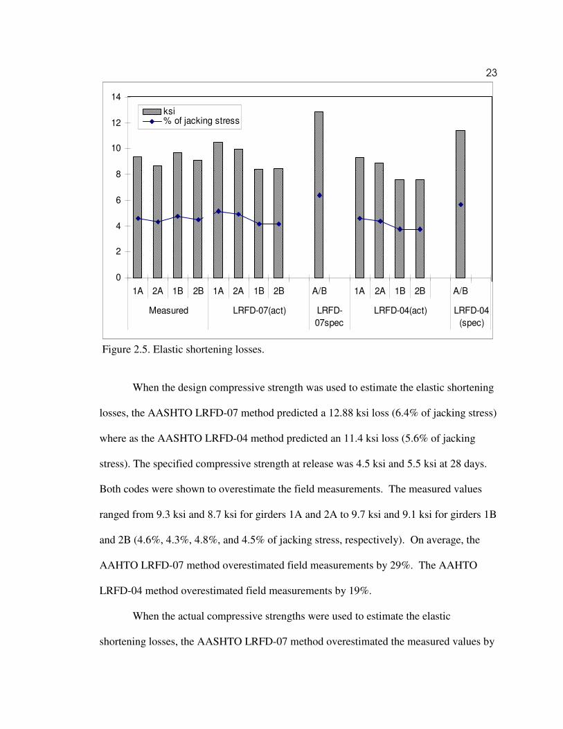
Figure 2.5. Elastic shortening losses.

When the design compressive strength was used to estimate the elastic shortening

losses, the AASHTO LRFD-07 method predicted a 12.88 ksi loss (6.4% of jacking stress)

where as the AASHTO LRFD-04 method predicted an 11.4 ksi loss (5.6% of jacking

stress). The specified compressive strength at release was 4.5 ksi and 5.5 ksi at 28 days.

Both codes were shown to overestimate the field measurements. The measured values

ranged from 9.3 ksi and 8.7 ksi for girders 1A and 2A to 9.7 ksi and 9.1 ksi for girders 1B

and 2B (4.6%, 4.3%, 4.8%, and 4.5% of jacking stress, respectively). On average, the

AAHTO LRFD-07 method overestimated field measurements by 29%. The AAHTO

LRFD-04 method overestimated field measurements by 19%.

When the actual compressive strengths were used to estimate the elastic

shortening losses, the AASHTO LRFD-07 method overestimated the measured values by

0

2

4

6

8

10

12

14

1A 2A 1B 2B 1A 2A 1B 2B A/B 1A 2A 1B 2B A/B

Measured LRFD-07(act) LRFD-

07spec

LRFD-04(act) LRFD-04

(spec)

ksi% of jacking stress

24

1%, on average. The AASHTO LRFD-04 method underestimated the field

measurements by 10.2% on average. For the case when the specified concrete

compressive strength was used in the calculation of the modulus of elasticity the

difference between the measured and predicted was larger by approximately 25%. Here,

the calculated elastic shortening losses were larger than the measured losses. This is

presumably due to the underestimation of the actual modulus of elasticity.

Individually, values using the AASHTO LRFD-07 method were shown to

overestimate girders 1A and 2A by 10.6 and 12.8%, respectively. In contrast, girders 1B

and 2B were underestimated by 15.5 and 7.9% respectively. Similarly, using the

AASHTO LRFD-04 method, girders 1A, 1B and 2B were under-predicted by 0.5, 27.4,

and 19.2 percent. Only girder 2A was conservatively estimated using the LRFD method

(2.2%). Measured values for the elastic shortening losses were based on an average

change in strain readings just prior to the first strand being cut through the point in time

when the last strand was cut. This approach presented next for Girder 1A (Figure 2.6).

Three sets of data are presented in Figure 2.6; “1ABL” and “1ABR” is

representative of data collected from the strain gauges located to the left and right sides

of the centroid of the prestressing tendons, respectively. These two sets of data were

averaged together (“AVG ELS SHRT 1A”) when calculating the elastic shortening loss.

As evidenced from Figure 2.5, an average change in strain of 327.7 microstrain,

multiplied by the modulus of elasticity of the steel (28,500 ksi), results in an elastic

shortening loss of 9.3 ksi. Elastic shortening losses for the three remaining girders were

also solved for in such a manner.

25

Figure 2.6. Elastic shortening losses for girder 1A.

Figure 2.7 presents the temperature readings associated with the casting and

curing stages. As previously mentioned, each girder was instrumented with four strain

gauges with embedded thermistors. 1A BL and 1A BR reflects the strain gauges to the

left and right sides of the prestressing steel. Data sets for 1AGC and 1ACC are

representative of the strain gauges placed at the center of the web and near the top of the

web, respectively.

As anticipated, the strain gauges nearest the top reported the highest curing

temperatures. Similarly, the strain gauges located at the bottom of the girder reported the

lowest curing temperatures. Temperature readings were shown to stabilize after

approximately 80 hours, indicating that the hydration process was complete. Little

variance was noted between the gauges, indicating that a consistent concrete strength

could be achieved based with respect to curing. Typically, higher curing temperatures

produce a higher strength concrete.

26

The prestressing force continues to decrease with creep and shrinkage of the

concrete over time as well. Effects such as temperature losses and relaxation also occur,

but are not addressed in this study. Additionally, there is an increase in the prestressing

force during deck placement; this is because the strain in the prestressing strands

increases when the deck load is applied.

Because total strain is being measured, the effects due to creep and shrinkage,

can’t be segregated in the field measurements, and are consequently presented in terms of

a total loss. As will be shown, the deck placement did increase the prestressing force.

Predicted prestress losses are presented alongside of measured values over time for each

method in Figures 2.8 through 2.11.

Figure 2.7. Curing temperatures versus time of curing for girder 1A.

27

Figure 2.8 shows the total calculated prestress losses according to the AASHTO

LRFD-04 and AASHTO LRFD-07 methodologies using the actual and specified

compressive strengths at release. Up through deck placement and after deck casting, the

calculated values using the actual concrete compressive strengths corresponded more

closely to the measured results for both prediction methods. This figure also shows a

typical history of measured prestress losses over time. In general, the rate of prestress

losses was initially large and then decreased until deck casting at day 130.

After deck casting, the rate of prestress loss increased until approximately day

225, after which it leveled off. This increase in prestress losses after deck casting is

presumably due to differential shrinkage and was consistent for each of the instrumented

girders. This behavior is not exhibited through the AASHTO LRFD-2007 prediction

method (Figure 2.8). In all, 500 days worth of data were recorded and are presented.

0.00

0.02

0.04

0.06

0.08

0.10

0.12

0.14

0.16

0.18

0 100 200 300 400 500 600

Time (days)

Str

ess L

oss a

s P

erc

en

t o

f Jackin

g S

tress (

ksi)

1A Measured

2A Measured

1B Measured

2B Measured

AASHTO LRFD-07,act

AASHTO LRFD-2004, act

AASHTO LRFD-07, spec

AASHTO LRFD-04, spec

Figure 2.8. Prestress losses over time; measured and predicted values.

28

For the measured values presented in Figure 2.7, the average of the bottom left

and bottom right strain gauges (placed at the centroid of the prestressing strand) were

used for each field measurement. At first inspection it is apparent that two gaps in the

field data exist. The first gap of 10 days (days 82 through 92) was a direct result of the

time required to ship the girders from the precast yard and erect the girders on site. The

second gap in data of 18 days (days 146 to 164) was believed to be the result of a battery

disconnect during the construction process. As shown by the marked decrease in

prestress loss, deck placement was captured in its entirety. As of day 500, prestress

losses via measured values were 11.4% (23.13 ksi) of the jacking stress on average.

Individually, prestress losses as of day 500, expressed as a percentage of jacking stress,

are as follows: girder 1A 12% (24.34 ksi); girder 2A 11% (22.20 ksi); girder 1B 11%

(22.56 ksi); and girder 2B 11.6% (23.40 ksi).

The AASHTO LRFD-07 method is shown to more accurately estimate the

residual prestressing force after the deck is cast as well as when actual compressive

strengths are used. This method is intended for high-strength concrete bridge girders.

The specified values were not considered high strength. This leads to the overestimation

of various creep coefficients and the separation of approximately 4% of the jacking stress

(8 ksi) when compared to the plot using actual compressive strengths, on average. In

either instance, the results were shown to be conservative. Using the AASHTO LRFD-

07 method in conjunction with the actual compressive strengths for this girder, estimated

prestress losses at day 500 was approximately 12% of the jacking stress (23.85 ksi).

29

When specified compressive strengths were used in conjunction with this method, the

estimated prestress losses as of day 500 grew to 16% of the jacking stress ( 32.98 ksi).

Also shown in Figure 2.8 are the predicted losses using the AASHTO LRFD-04

method. This method provides reasonable estimates of the stress losses through day 75.

After this point in time, the calculated and measured values continue to diverge from one

another. As of day 500, prestress losses via measured values were 11.4% (23.13 ksi) of

the jacking stress on average, as was previously mentioned. Using the AASHTO LRFD-

04 method in conjunction with the actual compressive strengths for this girder, the

estimated prestress losses at day 500 was 15% of the jacking stress (30.5 ksi). When

specified compressive strengths were used in conjunction with the AASHTO LRFD, the

estimated prestress losses as of day 500 were determined to be 16% of the jacking stress

to (33.2 ksi).

The deck was cast on day 130 (Figure 2.9). As previously mentioned, when the

deck is cast there is a gain in the residual tendon stress. This is a result of the prestressing

steel elongating when an additional load is applied. Figure 2.8 presents the measured

prestress losses in comparison with the AASHTO LRFD-07 method near the time the

deck was placed (days 123 through 137). As shown in Figure 2.9, there is a loss in

“stress losses” at day 130. This constitutes a stress gain. Additionally, gains can be

noted when the future wearing surface and parapet are cast.

30

0.0

2.0

4.0

6.0

8.0

10.0

12.0

14.0

12

0

12

1

12

2

12

3

12

4

12

5

12

6

12

7

12

8

12

9

13

0

13

1

13

2

13

3

13

4

13

5

13

6

13

7

13

8

13

9

14

0

time (days)

str

es

s l

os

s a

s a

pe

rce

nt

of

jac

kin

g s

tre

ss

(%

)1A measured

2A measured

1B measured

2B measured

AASHTO LRFD-07

Figure 2.9. Stress losses at time of deck casting. Stress gains that result from the deck placement for the four measured girders are

as follows: girder 1A 0.8% (1.64 ksi); girder 2A 0.8% (1.78 ksi); girder 1B 1.3% (2.75

ksi); and girder 2B 1.1% (2.11 ksi). The AASHTO LRFD-07 method predicted a 0.5%

stress gain relative to the jacking stress (1.03 ksi). Because the AASHTO-LRFD-07

method overestimated the creep, shrinkage, and relaxation, prior to deck placement, the

total stress loss was overestimated by approximately 1.5% of the jacking stress.

Referring back to Figure2.7 it is shown that this overestimation in the first 130 days of

the bridge’s life resulted in very accurate prestress losses from days 130 through 500;

namely an overestimation of 6% of the measured values on average.

Figure 2.10 displays ratios of the average measured values to the average of each

of the prediction methods. Both prediction methods were shown to be conservative as all

31

ratios are less than one. Data reflects when actual and specified compressive concrete

strengths were used for each code. Additionally the data are separated into two division,

values prior to deck casting (day 130) and values after deck casting (day 130-500). The

NCHRP incorporates both actual and specified compressive strengths when compared to

the measured values.

Overall, the AASHTO LRFD-07 method was shown to produce the most realistic

prediction of prestress losses over time (91.5%), when actual concrete compressive

strengths were used. Through deck placement (day 130), the actual compressive

strengths were shown to overestimate the measured values by an average of 13% when

used in conjunction with this method. Similarly the AASHTO LRFD-04 method was

shown to overestimate the average measured prestress losses by 6 percent, using the

actual compressive strengths.

0.00

0.20

0.40

0.60

0.80

1.00

1.20

Measured/

LRFD-07

Measured/

LRFD-07

Measured/

LRFD-07

Measured/

LRFD-07

Measured/

LRFD-04

Measured/

LRFD-04

Measured/

LRFD-04

Measured/

LRFD-04

through 130 130-500 through 130 130-500 through 130 130-500 through 130 130-500

act. spec. act. spec.

Rati

o (

Measu

red

/Pre

dic

ted

)

Figure 2.10. Ratios of measured values to code estimates.

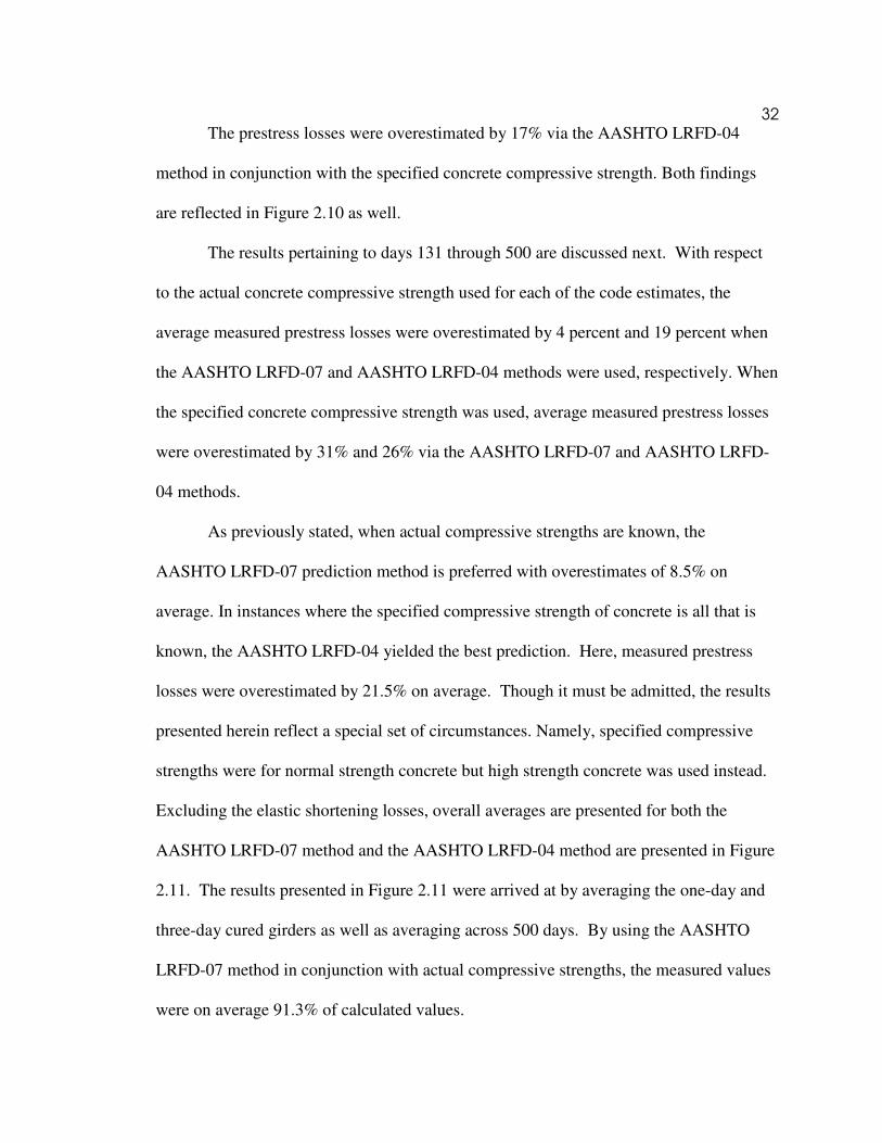
32

The prestress losses were overestimated by 17% via the AASHTO LRFD-04

method in conjunction with the specified concrete compressive strength. Both findings

are reflected in Figure 2.10 as well.

The results pertaining to days 131 through 500 are discussed next. With respect

to the actual concrete compressive strength used for each of the code estimates, the

average measured prestress losses were overestimated by 4 percent and 19 percent when

the AASHTO LRFD-07 and AASHTO LRFD-04 methods were used, respectively. When

the specified concrete compressive strength was used, average measured prestress losses

were overestimated by 31% and 26% via the AASHTO LRFD-07 and AASHTO LRFD-

04 methods.

As previously stated, when actual compressive strengths are known, the

AASHTO LRFD-07 prediction method is preferred with overestimates of 8.5% on

average. In instances where the specified compressive strength of concrete is all that is

known, the AASHTO LRFD-04 yielded the best prediction. Here, measured prestress

losses were overestimated by 21.5% on average. Though it must be admitted, the results

presented herein reflect a special set of circumstances. Namely, specified compressive

strengths were for normal strength concrete but high strength concrete was used instead.

Excluding the elastic shortening losses, overall averages are presented for both the

AASHTO LRFD-07 method and the AASHTO LRFD-04 method are presented in Figure

2.11. The results presented in Figure 2.11 were arrived at by averaging the one-day and

three-day cured girders as well as averaging across 500 days. By using the AASHTO

LRFD-07 method in conjunction with actual compressive strengths, the measured values

were on average 91.3% of calculated values.

33

0.0

10.0

20.0

30.0

40.0

50.0

60.0

70.0

80.0

90.0

100.0

Measured/

LRFD-07

Measured/

LRFD-07

Measured/

LRFD-04

Measured/

LRFD-04

act. spec. act. spec.

Rati

o

Figure 2.11. Comparison of overall averages.

In other words, the AASHTO LRFD-07 method overestimated the total prestress

losses by 8.7% on average. When specified compressive strengths were used under this

code, the AASHTO LRFD-07 method was shown to overestimate the measured values by

33%.

Using the AASHTO LRFD-04 method and the actual compressive strengths, this

approach overestimated the average measured values by 12.4%, compared to an average

overestimate of 21.6 percent when specified values were used. Based on these

percentages, the AASHTO LRFD-07 method is shown to more accurately predict

prestress losses. Overall trends indicate that this approach is conservative and that

predicted values converge towards measured values after deck placement. The measured

prestress losses for all four girders were predominantly overestimated during the first

phase of bridge construction. Both methods were shown to be conservative, when results

were averaged together.

34

Conclusions

Four precast, prestressed girders made with high-performance, self-consolidating

concrete were instrumented and monitored for prestress losses for 500 days since the time

of casting. The observed values of prestress losses were compared with values calculated

using the AASHTO LRFD-04 specifications and the AASHTO LRFD-07 specifications.

This study led to the following conclusions:

1) After 500 days worth of monitoring, the average measured prestress losses for

each of the four instrumented girders is approximately 20.89 ksi which

corresponds to a total loss of 10.3 percent of the jacking stress. This relatively

low percentage of total loss is due to a significantly higher concrete strength that

was required for the design.

2) In terms of elastic shortening losses, when using actual compressive strengths,

measured values on average, 99 percent of the AASHTO LRFD-07 predictions

and were 110 percent of AASHTO LRFD predictions. By using specified

compressive strengths (plan sheets), averages indicate measured E.S. losses were

now overestimated by 29 percent using NCHRP predictions, and overestimated

by 19 percent using AASHTO LRFD predictions.

3) When using actual compressive strengths, measured losses were on average

91.3% of the AASHTO LRFD-07 predictions and 87.6% of the AASHTO LRFD-

04 predictions (Both were conservative). Using specified compressive strengths

(plan sheets), measured losses were now 67.3% of the AASHTO LRFD-07

predictions and over-predicted by 78.4% of AASHTO LRFD-04 predictions (both

35

were conservative). Overall the NCHRP method proved to more closely

approximate measured values when actual compressive strengths were used.

4) At the time the deck was placed, an average gain of 1% of the jacking stress (2.1

ksi) was recorded for tendon stress. This compares to a gain of 0.5% using the

AASHTO LRFD-07 method.

5) With high-strength, self-consolidating concrete, compressive strengths were

observed to average 11.5 ksi at 28 days. The use of this type of concrete in

prestressed concrete bridge girders saves on time and money (as no vibration is

required).

36

CHAPTER 3

STRAIN ISOLATION IN CONCRETE CYLINDERS

Introduction

Research efforts summarized in chapter three (strain isolation in concrete

cylinders) was an important step in developing a non-destructive method to determine

residual tendon stress in prestressed concrete girders. The proposed method for

determining residual prestress involves isolating, but not removing, a small block on the

tensile face of a prestressed girder by making shallow cuts, freeing the block from

prestressing forces. The reduction of stress in the block should then be able to be related

to the effective prestress that is remaining in the girder.

A necessary initial component of this research involved modeling various

combinations of shallow cuts on four-inch diameter by eight-inch tall concrete cylinders.

By initially testing the cylinder, it was hoped to be able to determine the most efficient

combination of depth width and length of cuts with respect to the distance separating

those cuts in order to achieve a “near zero strain” over a specific region of the concrete

cylinder. Of all the possible combinations the most important parameter is the depth of

cut. This is because prestressing strands are typically located two inches from the outer

surface of a concrete girder. Therefore, we want the most efficient combination of cuts

while ensuring the depth of cuts is a safe distance away from the prestressing strands.

Accordingly, the purpose of this task was to determine how feasible and effective

it is to isolate a concrete block from a 4x8 concrete cylinder in order to obtain a near zero

strain. In addition, to quantifying the effect that various combinations of depth of cuts

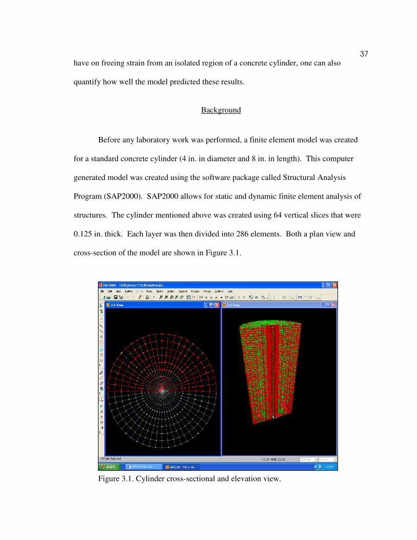
37

have on freeing strain from an isolated region of a concrete cylinder, one can also

quantify how well the model predicted these results.

Background

Before any laboratory work was performed, a finite element model was created

for a standard concrete cylinder (4 in. in diameter and 8 in. in length). This computer

generated model was created using the software package called Structural Analysis

Program (SAP2000). SAP2000 allows for static and dynamic finite element analysis of

structures. The cylinder mentioned above was created using 64 vertical slices that were

0.125 in. thick. Each layer was then divided into 286 elements. Both a plan view and

cross-section of the model are shown in Figure 3.1.

Figure 3.1. Cylinder cross-sectional and elevation view.

38

For this model, assumed material properties included the following:

1) A cylinder strength of 4,000 psi and

2) A static modulus of elasticity of 3.6E6 psi.

In all, 18,304 solid concrete elements (hereafter referred to as elements)

comprised this model. Each element can be thought of as a cube of specific dimensions.

Conceptually speaking, these small elements allowed for shallow cuts to be modeled in

increments of 0.25 in. depth-wise and length-wise as measured from the surface by

deleting an element or row of elements. Each layer was segmented to limit the aspect

ratios to 2:1 in any direction for the five outermost layers. (In addition to meeting an

aspect ratio of 2:1, cuts made at 0.25 in. intervals seemed to be reasonably easy to

achieve in the lab as well.) As shown in Figure 3.1, the innermost layer of elements

converges at a common center point. To this end, connectivity between all elements was

provided. In order to achieve optimal results both element connectivity and a limiting

aspect ratio of 2:1 are stipulated.

Again, it is important to note that the cuts imparted on the cylinder do not remove

a finite block from the cylinder but is intended to free it from the vertical stress imparted

on the surrounding body of the cylinder (in the direction of loading). As such, the

purpose of this model was to attempt to identify the parameters (depth, width, and length)

of two parallel cuts such that “zero stress” near the lengthwise center of the model

cylinder is observed-- when a uniform pressure (40% of the modeled cylinder strength, or

1,600 psi) is applied atop the cylinder. Forty percent of the modeled cylinder strength

ensured that cylinders would be loaded only in the elastic region of a stress strain

diagram. This is assuming that the actual concrete cylinders are at least as strong as the

39

modeled cylinders. This will be shown to be the case. As a direct result, laboratory

and equipment costs could were minimized as the cylinders could be retested with

different depth cuts.

When modeled, the cylinder is taken to be homogeneous and isotropic. However,

when experimentally determined, the cylinder may or may not be homogeneous and

isotropic depending on localized conditions. Accordingly, effects due to local variances,

such as aggregate near the surface, need to be minimized. Aggregate near the surface can

produce local stress concentration; thus data could be skewed. To minimize these effects,

strain values over a specified length were measured and averaged. The position and

location of these elements corresponded to the position and location of a strain gauge

placed on the cylinder for testing; thus the modeled results can be compared to the

experimentally determined results.

Sixteen of the centermost elements in the direction of loading were used to

calculate a “zero stress/strain” or as will be shown a “near-zero stress/strain.” “Zero

stress/strain” is calculated by averaging the surface stress/strain over a specified number

of elements in the direction of the applied load. Sixteen elements, corresponding to 2 in.,

were believed to be an appropriate length to average over. Aggregate can produce

localized stress concentrations if near the surface. To minimize localized effects due to

aggregate near the surface or any surface abnormalities such as air pockets that may be

present, the length one averages over needs to exceed the diameter of aggregate;

otherwise, data may be compromised. For this particular task strain gauges exceeded 2.5

times the diameter of 0.75 in. aggregate. Figure 3.2 shows the typical strain gauges used

in this experiment.

40

Figure 3.2. Strain gauges. The strain gauges pictured above are two-inch uniaxial strain gauges. The overall

“matrix length,” as it is called, is 2.5 in. long. An additional 0.25 in. buffer was allotted

to each side of the gauge to prevent damage when cuts were being placed. This meant

that at best, cuts could be placed no closer than 2.5 in. from the end of each cylinder.

Since preliminary finite-element results indicated that “zero stresses” or “near zero

stresses” were obtained when cuts were placed nearest the gauge, and parallel cuts could

not be placed closer than 2.5 in. from each end of the cylinder (or 3 in. from one another).

This placement fixed the offset distance. From here, various widths and depths were

modeled to determine the length and width of cuts. Each cylinder was equipped with two

strain gauges; one strain gauge was positioned between the paired cuts. The other strain

gauge was placed directly opposite the first one. To this end, the average from two strain

gauges could be used when calculating the static compressive modulus to determine how

comparable the cylinders are. Figure 3.3 shows how these cuts were made with the

available equipment.

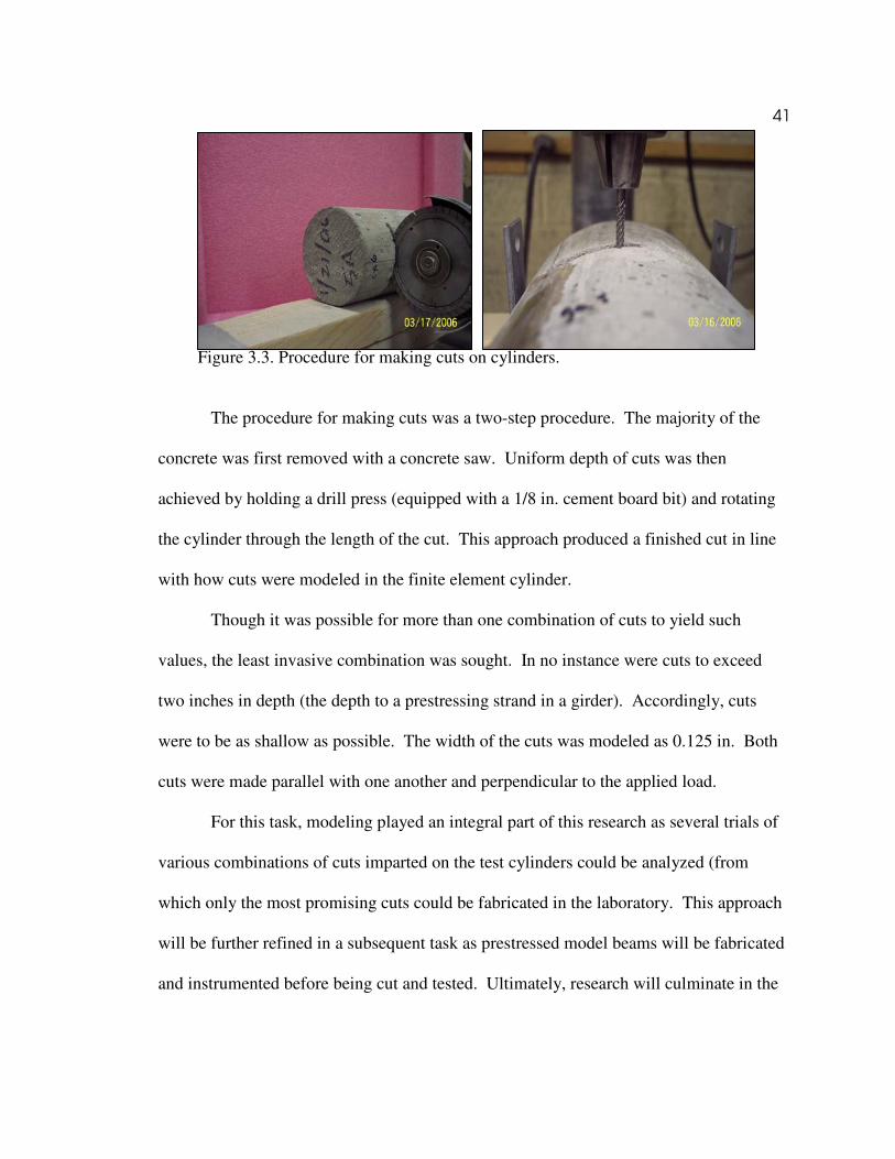
41

Figure 3.3. Procedure for making cuts on cylinders.

The procedure for making cuts was a two-step procedure. The majority of the

concrete was first removed with a concrete saw. Uniform depth of cuts was then

achieved by holding a drill press (equipped with a 1/8 in. cement board bit) and rotating

the cylinder through the length of the cut. This approach produced a finished cut in line

with how cuts were modeled in the finite element cylinder.

Though it was possible for more than one combination of cuts to yield such

values, the least invasive combination was sought. In no instance were cuts to exceed

two inches in depth (the depth to a prestressing strand in a girder). Accordingly, cuts

were to be as shallow as possible. The width of the cuts was modeled as 0.125 in. Both

cuts were made parallel with one another and perpendicular to the applied load.

For this task, modeling played an integral part of this research as several trials of

various combinations of cuts imparted on the test cylinders could be analyzed (from

which only the most promising cuts could be fabricated in the laboratory. This approach

will be further refined in a subsequent task as prestressed model beams will be fabricated

and instrumented before being cut and tested. Ultimately, research will culminate in the

42

full scale testing of eight prestressed girders salvaged from the I-15 reconstruction

project in Utah.

Objective

The objective of this task is to determine how feasible and effective it is to isolate

a concrete block from a 4x8 concrete cylinder in order to obtain a near zero strain on the

surface for an applied load. In addition to quantifying the effect that various

combinations of cuts have on freeing strain from an isolated region of a concrete

cylinder, one can also quantify how well the model predicted these results.

Equipment

a. (1) Vishay 5100B Scanner(Fig. 3.4)

b. (1) Tinius Olsen (Fig. 3.5)

c. (1) Mercoid Control, load restraint (Fig. 3.6)

d. (1) CLC-50k Transducer, Load Transducer (Fig. 3.7)

e. (1) P.C.

f. (3) 8” x 4”θ instrumented & cut concrete cylinder (Fig. 3.8)

g. (6) Strain gauges (Fig. 3.9)

h. (7) Instrument cards (Fig. 3.10)

43

Figure 3.4. Vishay system analyzer.

Figure 3.5. Tinius Olsen hydraulic testing machine.

Figure 3.6. Load restraint.

44

Figure 3.7. Load transducer.

Figure 3.8. Cylinder with strain gauge.

Figure 3.9. Strain gauges.

45

Figure 3.10. Instrument cards.

Procedures

For this particular experiment, three cylinders were loaded to 1600 psi, as

controlled by the load restraint, strain readings were recorded throughout the duration of

each test. The Tinius Olsen Universal tester was loaded at a uniform rate near 100

pounds per second. A calibrated load cell was used to accurately determine the load

applied. Both the load cell and strain gauges were wired into the Vishay system analyzer

using instrument cards such that readings were collected simultaneously. Readings were

collected at the rate of ten values per second. Various depths and separation of cuts were

explored. These parameters along with cylinder dimensions and weights are presented

next in Table 3.1. As indicated in Table 3.1, cylinders one through three were duplicates

of one another as each pair of cuts were located 2.5 in. from either end of the cylinder.

Similarly, cylinders four through six were cylinders whose pairs of cuts were made 2 in.

from either end. Cylinders seven through nine include those cylinders whose pairs of

cuts were located 2 in. from either end. Cylinders 1, 6, and 8 (one from each group) are

represented in the Figures 3.10 through 3.12.

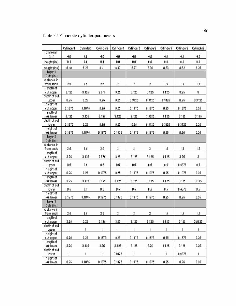
46

Table 3.1 Concrete cylinder parameters

47

97.7 95.9

0

20

40

60

80

100

% reduction in

strain

SAP Model Experimental

Reduction in Strain; Modeled vs. Experimental

Results

For this experiment, the ultimate goal is to compare the reduction in strain

resulting from the various cuts to 1) cylinders with no cuts 2) to one another as well as 3)

to the predicted strains using SAP (when provided). When making comparisons between

cylinders 1 through 9, measurements from ten load intervals ranging from 2,000 to

20,000 lbs, were recorded. All load intervals fell within the elastic region of each

concrete cylinder. The ideal result was to obtain a cut configuration that resulted in a

“zero strain” reading as the loading was increased to 1600 psi. This level of stress

corresponded to modeled results that at 1600 psi (roughly 20,100 lbs load) produced a

strain reduction of 97.7% (see Figure 3.11). Actual results fell within two percent of this

value when compared to cylinder one. When results from cylinders one through three

were averaged together, modeled and experimental results were within 1.3% of one

another (average experimental value of 96.4%).

Figure 3.11. Modeled vs. experimental results of optimally placed cuts for cylinder 1.

48

These results indicate two very important findings: First, the computer model

serves as a good predictor both in terms of optimizing the placement and depth of cuts

and isolating a stress block; second, this approach is promising in terms of ultimately

estimating residual prestress in prestressed concrete girders. In fact, for the optimally

placed cuts (3 in. from one another), results were uniform throughout the duration of

loading (Figure 3.12).

Cuts placed on cylinder one are optimized in terms of spacing (0.5 in. from either

end of the strain gauge), and length (3.125 in.). The depths of cuts ranged from 0.25

inches at layer one to 0.5 in. at layer two and were optimized for layer three where a

depth of 1 in. was achieved. Recall cut optimization was predetermined in the computer

model; refer to Table 3.1. Figure 3.12 shows that a 20% reduction in strain was achieved

from 5,000 lbs through a maximum load of 20,000 lbs.

86.386.0

89.791.6

92.794.0

94.594.9

95.595.9

-60.0

-40.0

-20.0

0.0

20.0

40.0

60.0

80.0

100.0

0 5000 10000 15000 20000 25000

load (lbs)

% r

ed

uc

tio

n o

f s

tra

in

layer 1 cuts

layer 2 cuts

layer 3 cuts

Figure 3.12. Reducing strain from cylinder 1 tests.

49

Meanwhile, results for the layer two cuts ranged from 20 percent near a load

of 5,000 lbs to 40 percent when the load was increased to 20,000 lbs. A dramatic jump

occurred at layer three. Here, over 90 percent reductions in strain were achieved over 70

percent of the load intervals. A maximum reduction of 95.9 percent occurred near 20,000

lbs load (roughly 1600 psi). When the layer three cuts for cylinders one through three

were averaged together, a strain reduction of 96.4 percent was achieved. These effects

diminished with an increased separation of cuts (Figures 3.13 and 3.14). Figure 3.13

presents findings for cylinder six. Cuts were placed one inch from either end of the strain

gauge.

As shown in Figure 3.13, both the first and second layer cuts fell below 20%

reduction; this was to be expected, as neither were at the optimum depth or distance

apart. For the 1 in. deep cuts, strain reduction ranged from 36.2% to 51.5% when

compared to the uncut scenario. This is approximately 40% less than the optimized cuts

placed 0.5 in. from either end of the strain gauge.

40.336.2

37.7

40.7

44.947.0

49.250.2

51.151.5

-60.0

-40.0

-20.0

0.0

20.0

40.0

60.0

80.0

100.0

0 5000 10000 15000 20000 25000

load (lbs)

% r

ed

ucti

on

of

str

ain

layer 1 cuts

layer 2 cuts

layer 3 cuts

Figure 3.13. Effect of increased cut spacings (1 inch) from cylinder 6 tests.

50

When cylinders 4 through 6 were averaged together, an average reduction of

47.3% was obtained for the layer-three cuts. Furthest from the overall goal of a 100%

reduction in strain were the results from cuts placed 1.5 in. away from either end of the

strain gauge (see Figure 3.14).

Here the first two layers of cuts show higher reported strains over the entire load

interval. Strain reduction in layer three cuts ranged from a five percent near 7,500 lbs

load to 21.9% near 17,500 lbs load for cylinder eight. Averages are not presented for this

group of cylinders, as higher loads resulted in failed cylinders.

It can be concluded that based on the results from this series of tests it is apparent

that 95% reductions are possible. However, the depth and placement of cuts is critical in

achieving such reductions in strain. Thus, when separating the cuts by as little as 0.5 in.

more than the optimum spacing or cutting to within 0.5 in. of the specified depth

produces less than desirable results.

-8.3

-3.3-0.4

5.0

10.6

14.817.8

20.321.9

-80.0

-60.0

-40.0

-20.0

0.0

20.0

40.0

60.0

80.0

100.0

0 5000 10000 15000 20000 25000

load (lbs)

% r

ed

uc

tio

n o

f s

tra

in

layer 1 cuts

layer 2 cuts

layer 3 cuts

Figure 3.14. Effect of increased cut spacings (1.5 inch) from cylinder 8 tests.

51

For this task each cylinder was instrumented with two strain gauges, placed on

opposing ends. Compressive tests were run on cylinders cast from the same batch of

concrete, to verify that each “instrumented” cylinder was well within the elastic region

when loaded. Results from each strain gauge were then averaged together and plotted

against the pressure arrived at through the calibrated load cell. A trend line was fit to the

data and the resulting slope of each line represented the modulus of elasticity of each

cylinder. The results are summarized in Table 3.2; raw data is included in Appendix A.

The fact that all cylinders tested in this experiment exhibited similar compressive

modulii, and were cast from the same batch of concrete is an indicator that results are

comparable.

Conclusions

Results indicate that a 95.9% reduction in strain was achieved at a load of 20,000

lbs on a 4x8 inch cylinder. Measured and predicted strains are within 2% of one another

for the optimized pair of cuts. This means that the computer model served as a accurate

predictor; both in terms of optimizing the placement and depth of cuts and isolating a

stress block. The optimum pair of cuts (as they have been termed) occurs when the

following three conditions are met:

1) Cuts are centered 0.5 in. from either end of the two-inch strain gauge. The matrix

length of the strain gauge is 2.5 in. long. However, the gauge itself is two inches

in length. Accordingly, the latter dimension serves as the reference point for the

parallel cuts;

2) Cuts penetrate the cylinder to a depth of 1 in.; and

52

3) Cuts are 3.125 in. long.

Comparisons made between the cylinders show that when paired cuts are placed further

apart from the strain gauge, strain within the isolated block increased. This finding was

also the case for cuts less than 1 in. deep. Results from this task indicate that much

promise exists in terms of accurately estimating residual prestress in prestressed concrete

girders.

Table 3.2. Compressive modulus of elasticity (psi)

Cylinder 1 Cylinder 2 Cylinder 3 AVG

4372709 4359468 4754341 4495506

Cylinder 4 Cylinder 5 Cylinder 6 AVG

4042294 4480615 4133141 4218683

Cylinder 7 Cylinder 8 Cylinder 9 AVG

4311455 4132531 4310822 4251603

53

CHAPTER 4

MODEL BEAM TESTS

Introduction

This portion of the research presents the development of a testing protocol for

small prestressed concrete beams; the creation of finite-element models used to optimize

the placement of cuts; prestressed beam fabrication, laboratory testing; and finally data

analysis.

Background

One 32-foot long beam was cast at Encon Precast in the stem of a double T

section. The beam was cast the first day and de-stressed approximately 24 hours later.

Over the course of the next week the 32-foot section cured uncovered in a sand bed.

Then the beam was saw cut into four, 8-foot lengths. Of the four beams, two beams

incorporated two prestressing strands, and two beams incorporated three prestressing

strands. This change in quantity of strands was accomplished by de-bonding the center

strand over 16 of the 32 total feet. A jacking stress of 29,800 lbs was introduced into

each of the ½ in. nominal diameter, 7-strand cables.

Laboratory preparation for the prestressed beam tests involved purchasing and/or

procuring the following items for testing: 350 ohm uniaxial strain gauges, a 50,000 pound

capacity load cell, a hydraulic load frame, and beam supports.

54

Five strain gauges were allotted for each of the four prestressed beams. After

each beam was initially cracked, strain gauges were affixed to the tension face of each

beam and were used to experimentally determine the decompression load for each beam.

Procedure and Interim Results

The approach for this portion of the research was to crack first, instrument

second, and place cuts third. To this end, the beam(s) would be cracked in an unaltered

state. The prestress force can then be determined and incorporated into a finite-element

model. At this point the length and depth of cuts, necessary to free up the residual

compression strain could be determined. The magnitude of this compressive strain will

then be used to validate the prestress force used in the model. If the prestress force

arrived at through cracking the beam agrees with the prestress force arrived at through the

strain isolation, then collectively, each approach can be validated.

Determining the decompression load

Beams were initially cracked by means of applying a single load evenly

distributed across the width of the beam at mid-span as shown in Figure 4.1. A single

load was preferred because it was believed to limit both the location and number of

cracks that would form as a result of loading. In turn, this meant that fewer cracks

needed to be instrumented on any given beam. A cross-section of this beam is also

included in Figure 4.1. The cross sectional area of each beam was 42.5 in. with a

centroid of 3.9 in., as measured from the bottom of the beam.

55

Figure 4.1. Beam loading setup and cross section.

The concentrated load was applied hydraulically at a rate not in excess of 50

pounds per second. Once cracking was noticed, the load was increased until cracking

propagated from the tensile face up to the centroid of the prestressing strands. At this

point the load was held constant and the crack was traced using a permanent marker.

(Note: had the load been removed prior to identifying the crack, the crack would not have

been visible to the unaided eye.) Loading was discontinued at approximately 5000 lbs for

each two strand beams and at approximately 6000 lbs for each three strand beam.

Strain gauges were then affixed to the tension face of the beam in accordance with

the crack pattern. Strain gauges were placed directly to either side of the crack and

another strain gauge was positioned directly over the crack (Figure 4.2). Once

instrumented, each beam was loaded to a value of approximately twice the

decompression load. Values of microstrain and applied load were recorded at the rate of

one scan per second throughout the duration of each test. Using the recorded data, the

corresponding decompression loads were determined graphically.

56

For this particular set of tests the strain gauges were zeroed and calibrated

when the beam was placed atop the supports. Additionally, the strain gauges were

affixed to the beams after the prestressing force was introduced. For these reasons, the

reported values of strain do not correspond to the anticipated values of strain outright.

The latter would have been observed had the gauges been affixed prior to de-stressing the

prestressed strands and imposing the weight of each beam. Data collected during the

decompression tests for each of the two-strand beams are presented in Figure 4.3.

Microstrain values corresponding to the strain gauges placed to the left and right of

beams one and two reference the leftmost “y axis”. Microstrain values corresponding to

strain gauges placed directly over the crack(s) reference the right-most axis in Figure 4.3.

In terms of behavior, the strain gauge placed directly over the crack increased

linearly with the applied load until the crack opens. Strain gauges placed to either side of

the crack were expected to exhibit a bilinear response. As shown in Figure 4.3, there is

close agreement between the strain gauges placed directly over the cracks for beams one

and two. A bilinear response was not observed for any of the left and right strain gauges.

Data collected during the decompression tests for each of the three-strand beams are

presented in the Figure 4.4. The strain gauge placed directly over the crack for beams

three and four also increased linearly with the applied load until the crack opened.

Of the three-strand beams, only beam four was instrumented to the left and right

of the crack in addition to over the crack. After carefully considering various options, it

was decided that the strain gauges placed over the crack would be used in determining

the decompression loads for each of the beams.

57

Figure 4.2. Strain gauge placement.

0

50

100

150

200

250

300

350

0 1000 2000 3000 4000 5000 6000

Load (lbs)

Ad

jac

en

t M

icro

str

ain

0

1000

2000

3000

4000

5000

6000

Cra

ck

mic

ros

tra

in

left beam 2

right beam 2

left beam 1

right beam 1

beam 2 o.c.

beam 1o.c.

Figure 4.3. Decompression loads for two-strand beams.

58

0

50

100

150

200

250

300

0 1000 2000 3000 4000 5000 6000

Load (lbs)

Ad

jac

en

t m

icro

str

ain

0

1000

2000

3000

4000

5000

6000

Cra

ck

mic

ros

tra

in

Right Beam 4

Left Beam 4

Beam 4 O.C.

Beam 3 O.C.

Figure 4.4. Decompression loads for three-strand beams. Straight lines were fit to the data points in the linear region. The data point just

prior to deviation from this line was used to identify the decompression load. Figures 4.5

through 4.8 present the respective decompression load for beams one and two (the two

strand beams) as well as beams 3 and 4 (the three strand beams).

Using this approach, Figures 4.5 and 4.6 display results from the decompression

tests for beams one and two. Each two-strand beam produced equivalent decompression

loads of 1600 pounds. Similarly, Figures 4.7 and 4.8 display results from the

decompression tests for beams 3 and 4. Each three-strand beam produced equivalent

decompression loads of 2500 pounds. All tests were conducted independent of one

another. Over the linear portion of each curve the data points were nearly

indistinguishable (Figures 4.3 and 4.4).

59

Figure 4.5. Decompression load, beam 1 (2 strands).

Figure 4.6. Decompression load, beam 2 (2 strands).

Decompression Load

Encon Beam 1 (2 strands)

0

1000

2000

3000

4000

5000

6000

0 1000 2000 3000 4000 5000 6000

Load (lbs)

mic

rostr

ain

beam 1o.c.

Decompression

load 1600 lbs

Decompression Load

Encon Beam 2 (2 strands)

0

1000

2000

3000

4000

5000

6000

0 1000 2000 3000 4000 5000 6000

Load (lbs)

mic

ros

tra

in

beam 2 o.c.

Decompression

load 1600 lbs

60

Figure 4.7. Decompression load, beam 3 (3 strands).

Figure 4.8. Decompression load, beam 4 (3 strands).

Decompression Load

Encon Beam 3 (3 strands)

0

1000

2000

3000

4000

5000

6000

0 1000 2000 3000 4000 5000 6000

Load (lbs)

mic

ros

tra

in

Beam 3 Over Crack S.G.

decompression load 2500

pounds

Decompression Load

Encon Beam 4 (3-Strand)

0

1000

2000

3000

0 1000 2000 3000 4000 5000 6000

Load (lbs)

mic

rostr

ain

Beam 4 O.C.

Decompression

load 2500 lbs

61

Determining the residual prestressing force

Once the decompression load and similar section properties were obtained, the

corresponding residual prestress force for each beam was determined through the

following set of equations:

(4.1)

here:

F= the stress at the crack location

Pe = the effective prestress force

A = the gross cross sectional area of the beam

e = eccentricity of prestress force from the centroid

yt = distance from the crack on the bottom surface of the beam to the centroid

r = the radius of gyration

Mt = the total moment at the lengthwise position where the crack is located

here:

Mt = (Mdl + Mdec) (4.2)

here:

Mdl = the beam self-weight moment at the lengthwise position where the crack is

Mdec = the moment due to the applied decompression load where the crack is

Mdec = ½ (Pdecx) (4.3)

Pdec = the applied load at decompression

x = the distance from the crack position to the nearest support

62

This procedure was adopted from the methodology presented in the work of

Pessiki, Kaczinski, and Wescott (1996). As stated in their work, it is important to point

out that at decompression F= 0. Hence, the effective prestress force can be solved for

directly at this point.

Table 4.1 summarizes the section properties and variables used in solving

equations a, b, and c along with the prestress force and prestress loss for beam one, the

first of the two strand beams to be tested.

Table 4.1. Beam 1 section properties and variables

63

Interim Results

The prestress loss for beam one was determined to be 22.1% of the jacking stress.

The residual prestressing force for beam one was experimentally determined to be 23,

229 pounds per strand. All beams were cast in a single pour. As such each beam had

uniform section properties. The prestress loss for the remaining beams was solved for in a

similar fashion. The residual prestressing force and prestress loss for each beam are

presented in Figure 4.9.

As shown in Figure 4.9, the residual prestressing force for beam two was

determined to be 23,667 pounds per strand. The loss for beam two was determined to be

20.6% of the jacking stress. As previously mentioned, each of the beams had identical

section properties. The small difference that exists between the two-strand beams are

attributed to the fact that beam 2 cracked a distance of 35.2 in. (0.7 in. further) from the

nearest support.

Figure 4.9. Prestressing force and prestress loss per strand.

64

Values presented in Figure 4.9 for beams three and four indicate that both

beams were in agreement. This is attributed to similar section properties, decompression

loads and cracking locations. The residual prestressing force for each of the three strand

beams was determined to be 23,580 pounds per strand. The percent loss at the time of

testing for beams 3 and 4 were 20.9%. The residual prestressing force and prestress

losses for all four beams were within two percent of one another. These findings indicate

that the approach used to determine the residual prestress force is valid.

The average prestressing force of approximately 23, 450 pounds per strand was

used for the “two-strand beam” computer simulations, even though either prestressing

force would have produced nearly identical results (where residual strain on the tensile

face of the beams is concerned). To maintain consistency with the experimental results

for beams three and four a prestressing force of 23,580 pounds per strand was used for

the “three-strand beam” computer simulations.

Computer simulation and secondary findings

Once the prestressing forces for the two strand and three strand beams were

known, computer simulations could be run to isolate a combination of cuts that would

free the stress block of any residual compressive strain and ultimately be able to provide

the necessary information to calculate the residual prestressing force.

As with the concrete cylinders, a finite-element model was created for the beams

tested during this phase of the research. The beam mentioned above was created using 64,

1 in. layers to either end and one hundred and twenty-eight 0.25 in. layers over the

65

centermost portion of the beam. Each layer was then divided into 208 elements. The

end view of this three-dimensional model is presented in Figure 4.10.

Figure 4.10. The end view of the three dimensional model.

66

-127 -124-136

-196 -194-213

-250

-200

-150

-100

-50

0

comp. simulation hand calcs (comp.

dim.)

hand calcs (act.

dim.)

mic

ro-s

train

2-strand 3-strand

The solid element and cable elements were used to create a 3-D rendering of the

beams tested in the laboratory. Aspect ratios of less than or equal to “4” were used to

optimize the computer results. The computer model was created to the following three

dimensions:

1) cross-sectional area of 41.875 in.2;

2) moment of inertia of 145.17 in. 4; and

3) eccentricity of -0.48 in.

Actual beam dimensions were as follows: cross sectional area of 42.48 in.,

moment of inertia of 151.9 in., and an eccentricity of -0.4125 in.

Three groups of 8, 0.25 in. elements were designated at specific locations. Each

group was used to simulate each of the 2-inch strain gauges that were instrumented on the

actual girders. Eight elements, corresponding to 2-inches, were believed to be an

appropriate length to average over. Computer simulations were verified with hand

calculations. The results from each are presented below in Figure 4.11.

Figure 4.11. Computer simulations versus hand calculations.

67

The two-strand beams will be discussed first. Figure 4.11 shows that the

computer simulation was within 2.5% of hand calculations when using the dimensions

used for the computer simulations. When actual dimensions were used, the computer

simulation was within 6.6% of hand calculations. In terms of the three-strand beams,

results show that the computer simulation and hand calculations were within one percent

of one another when the computer simulation dimensions were used. When actual

dimensions were used for the hand calculations, values fell to within nine percent of one

another. The values presented in Figure 4.11 were all based on a modulus of elasticity of

4,527 ksi (Appendix A).

The computer simulations were slightly more conservative than the hand

calculations (based on actual dimensions). As such, the computer simulations became the

bench mark for determining when a particular combination of cuts was effective in

freeing a stress block from target values of compressive strain. Hence the target value for

the two strand beams was 127 microstrain (compression). Similarly, the target value for

the three strand beams was 196 microstrain (compression).

Placing cuts to either side of a strain gauge in computer simulations proved to be

ineffective in freeing tensile strains from the tension face of beams (Figure 4.12).

However, when the cumulative strain was in compression (i.e. the compressive strain

from the prestressing force was larger than the tensile strain due to self weight), the

computer simulations were effective in freeing residual strain as was previously shown

in Figure 4.11. External loading was omitted from the prestressed concrete beams

simulated in the computer and tested in the laboratory. This was to maximize the

observed compressive strains as they are so small to begin with (Figure 4.11).

68

For the five depths plotted in Figure 4.12, residual tensile strain was greater

than zero. For a scenario such as this, computer simulations were run with the beam

under self weight, a prestressing force, and a four-point loading large enough to produce

tensile strains at the specified strain gauge locations. All cuts were based on a pair of cuts

three inches long spaced 3 inches apart from one another.

A modulus of 4527 ksi was used in calculating microstrain under a four-point

load of 1200 lbs. This loading produced a decompression moment close to the

decompression moment observed on beam one (Table 4.1). The decompression moment

is the value corresponding to a load at which the crack opened on an instrumented beam.

Of the actual beams tested in the laboratory strain gauges were placed six inches from

mid-span; one to either side at the width-wise center on the tension side of all beams.

Figure 4.12. Residual tensile strain.

69

Computer simulations run on the two-strand beams confirmed that placing the

gauges 12 in. from one another eliminated the possibility of one set of cuts having

influence over the other adjacent pair of cuts. The next two figures represent some of the

scenarios that were explored when isolating the cuts. Figure 4.13 shows lengths effect on

freeing residual strain near the target value. The target combination of cuts is identified as

the combination that produces a stress nearest zero over a specified gauge length. In our

case, the gauge length was 2 in. For convenience, values were then converted to

microstrain. This is because the actual beams instrumented with uniaxial strain gauges

read in such units.

Figure 4.13. Length of cut versus simulated strain readings for the two-strand beams.

Length of Cut vs. Microstrain, 2strand beams

-4.2

5.65

10.4

-6

-4

-2

0

2

4

6

8

10

12

0 0.5 1 1.5 2 2.5 3 3.5

Length of Cut (in)

mic

ros

tra

in

length = varries

separation = 3 in

width = 0.25 in

depth = 0.75 in

prestress = 23.450 kips

70

Based on these computer simulations, an effective combination proved to be a

pair of ¼ in. wide cuts made ¾ in. deep, 2 ¼ in. long, with three inches of separation. For

this combination of cuts, an observed tensile strain of 5.65 microstrain was observed in

the computer simulation. Prior to simulating the cuts a compressive strain of 127 was

present at the designated strain gauge locations in the computer model.

As shown in Figure 4.13, values ranged from -4.2 microstrain to 10.4 microstrain

when the length of cut was adjusted from 2 in. to 3 in. long. All other parameters were

held constant. Parameters for these cuts include 3-inches of separation, ¼ -inch wide,

and ¾ -inch deep. Values reflect a prestressing force of 23.45 kips. Figure 4.14 shows

the effect varying the depth of cuts has on residual microstrain near the target

combination. Here the length of cuts was 3 in. long, three inches apart, and were ¼-inch

wide.

Figure 4.14. Depth of cut versus simulated strain readings for the two strand beams.

71

As shown in Figure 4.14, values ranged from -81 microstrain to 10.4

microstrain when the length of cut was adjusted from ¼ in. deep on up to ¾ in. deep. All

other parameters were held constant. The depth of the cut was shown to have had a

greater influence than did the length of the cut. It was necessary to manipulate both

parameters to optimize the cuts as shown in Figures 4.13 and 4.14.

Results, stress block isolation, two-strand beams

Armed with the target combination the next step was to reproduce these cuts on

the two strand beams in the laboratory (Figure 4.15). The saw cuts were performed with

an electric hand-held grinder. This grinder was equipped with a 4-inch diameter

diamond-tipped blade. Multiple saw cuts were made to achieve a consistent depth. Each

pair of saw cuts was then cleaned out with a dremmel tool and a tile cutting bit. This

helped to insure that a consistent depth of cut was achieved across the entire width of the

member. As such, this proved to be a very time-consuming and required some effort.

However, the target parameters were achieved for the length, width and spacing of cuts.

Results for the two-strand beams are summarized in Figure Table 4.2.

Figure 4.15. Isolating a stress block.

72

Table 4.2. Results for 2-strand beams 2-strand Beams ustrain

comp. simulation 127

hand calcs (comp. dim.) 124

hand calcs (act. dim.) 136

Beam 1 cuts sg ustrain % of c.s. % hand c.s. % of hand act.

1/4 deep 21/2 long 46 36 37 34

5/16 deep 2 1/2 long 101 80 81 74

3/4 deep 2 1/2 long 114 90 92 84

3/4 in deep 2 3/4 in long 139 109 112 102

Beam 1 no cuts sg ustrain % of c.s. % hand c.s. % of hand act.

5/16 deep 2 1/2 long 30 24 24 22

3/4 deep 2 3/4 long 77 61 62 57

1deep a.t.w. 128 101 103 94

removed 298 235 240 219

Beam 2 cuts sg ustrain % of c.s. % hand c.s. % of hand act.

1/2 deep 2 1/2 long 40 31 32 29

3/4 deep 2 1/2 long 67 53 54 49 3/4 deep all the way across 78 61 63 57

Beam 2 no cuts sg ustrain % of c.s. % hand c.s. % of hand act.

1/4 in deep 2 1/2 long 10 8 8 7 3/4 in deep all the way across 43 34 35 32

Table 4.2 presents the results for all of the experimentally determined

combination of cuts and compares them to the target values that were previously

presented in Figure 4.11. For the target combination of cuts (3/4-in. deep, 2.25-in. long),

beam one was 90% of the value predicted by the computer simulation when the first pair

of cuts reached the target combination. As for the second pair of cuts placed on beam

one, only 67% of the computer simulation value was reached. For this strain gauge, only

when the cuts reached a depth of 1 in. and the length of cuts spanned the entire width of

the beam were the target value and experimental values in agreement.

73

Results for beam two were 53% of the computer simulated value when the

target combination of cuts was reached. There was no combination of cuts for beam 2

that brought experimental and predicted values within an acceptable range of 10% or less.

Upon placing the target cuts on each of the beams, a four-point load was applied

to beam one. Results for the four-point load are presented in Figure 4.16. For beam 1,

the strain gauge that came within ten percent of predicted values was selected for

evaluation here. When a constant moment was applied, after the target depth of cuts was

placed, the general trend indicated that further increasing tensile strains were observed

(Figure 4.16). This indicates that on actual beams tested, 1) the target cuts are valid so

long as the loading does not change significantly due to future wearing surface etc., and

2) even though an external load applied to a given beam would produce a smaller

compressive strain, results would most likely only be valid if the target cuts were made

after the fact. Of the two-strand beams tested, only one of the four strain gauges produced

results that were in agreement with the predicted values.

Figure 4.16. Four-point load applied after target cuts for beam 1.

74

For this reason, a more in depth analysis was carried out and the experimental

plan was modified slightly to determine if cracking the beams prior to placing cuts on the

beam had any bearing on the results. A discussion of the three-strand beams follows.

Parametric study, three-strand beams

Upon testing the two-strand beams, it was decided that a more in depth analysis

was required. First, a parametric study was carried out through a series of computer

simulations. These computer simulations explored the effect that the length, width,

separation, and depth of cuts had on freeing a stress block from the residual strain beyond

the target combination. Additionally, the prestressing force was varied, and its effects on

simulated strain readings were noted. The experimental plan was also modified. Beam 3,

the first of the three-strand beams to be tested, was cut prior to cracking, while beam four

was cracked first prior to placing cuts. Results from both the parametric study and the

modified experimental plan are discussed next.

For the various scenario presented herein, three strain gauges were simulated in

the computer model. The “cuts” strain gauge represented the strain gauge situated

between the pair of cuts made to either end of the strain gauge. The “no cuts” strain

gauge was located directly opposite the cuts strain gauge. Aptly named, the “no cuts”

strain gauge did not have cuts placed to either end, during initial tests. Both strain gauges

are located six inches to either end of the mid-span. The center strain gauge was located

directly at mid-span of the beam. Both the center strain gauge and the “no cuts strain

gauge served as markers for this parametric study. In addition to providing baseline

values, one could see the effect the various combinations of cuts had while they were

75

some distance away from the isolated stress block. The first parameter to be explored

was the depth of cut in relation to freed microstrain. Results are presented below, in

Figure 4.17.

As shown in Figure 4.17, with no cuts placed to either side of the “cuts” strain

gauge, all three strain gauges were in agreement at -196 micostrain (196 compressive

microstrain). As the depth of cut varied from 0 inches to 1.5 in., the remaining

parameters were held constant: length of cut 2 ¼ in., separation between cuts 3 in., width

of cut ¼ inch, and prestressing force 23.580 kips per strand.

Figure 4.17. Depth of saw cuts versus microstrain.

76

At a depth of 0.75 in., the computer simulation estimated that three microstrain

are present over the computer-simulated strain gauge. As the depth of cut is increased

from 0.75 in. on up to 1.5 in., the simulated values reach approximately 30 microstrain

(tension). Both the “no cuts” and center strain gauges remain virtually unchanged

throughout the first 0.75 in.

The center strain gauge begins to deviate slightly from the baseline value after

0.75 inches, indicating that the last few combinations of cuts was having some influence

over the center strain gauge. Values based on the “no cuts” strain gauge remained

unchanged throughout this portion of the study. This indicates that at a distance of 12 in.

from the cuts strain gauge (center to center), adjacent strain readings were unaffected by

the depth of cut.

The second parameter to be explored was the length of cut in relation to freed

microstrain. Results are presented below, in Figure 4.18. As shown in Figure 4.18, with

no cuts placed to either side of the “cuts” strain gauge, all three strain gauges were in

close agreement. As the length of cut varied from zero inches to 6.5 inches (the entire

width of the beam) to either side of the cuts strain gauge, the remaining parameters were

held constant: depth of cut 0.75-in., separation between cuts 3-in., width of cut 0.25-in.,

prestressing force 23.5824 kips per strand.

Both the “no cuts” and center strain gauges remain virtually unchanged (within 2

microstrain) throughout the length of cuts when the other parameters are held constant.

This indicates that at a distance of 6 in. from the cuts strain gauge (center to center),

strain readings were unaffected by the length of cut. With that said, all other parameters

were held constant.

77

Figure 4.18. Length of saw cuts versus microstrain.

The third parameter to be explored was the separation between cuts in relation to

freed microstrain. Results are presented below, in Figure 4.19. As indicated in Figure

4.19, the distance separating the pair of cuts varied from 3 inches to 6 inches (centered at

the midpoint of cuts strain gauge). The remaining parameters were held constant: length

of cut 2.25-inches, width of cut 0.25-inches, depth of cut 0.75-inches, prestressing force

23.5824 kips per strand. At a separation of 3-in., the computer simulation estimated that

three microstrain are present over the computer-simulated strain gauge. As the separation

between the pair of cuts is increased from 3 in. up to 6 in., the “cuts” strain gauge fell to -

160 microstrain (160 compressive microstrain). This indicates that a separation of six

inches between the pair of cuts was effective in freeing 36 of the 196 microstrain. Only

the center strain gauge was affected by the separation of cuts.

Length of Cut vs Microstrain

-210

-200

-190

-180

-170

-160

-150

-140

-130

-120

-110

-100

-90

-80

-70

-60

-50

-40

-30

-20

-10

0

10

20

30

40

0 0.5 1 1.5 2 2.5 3 3.5 4 4.5 5 5.5 6 6.5

Length (in)

Mic

rostr

ain

cuts sg centersg

no cuts sg

length = varries as shown

separation =3 in

width = 0.25 in

depth =0.75 in

Prestress = 23.5824 Kips

78

Figure 4.19. Spacing between saw cuts versus microstrain.

The center strain gauge deviated from the baseline value by approximately ten

microstrain, when the separation of cuts was at six inches. This finding was somewhat

intuitive as the closer a saw cut is to an adjacent strain gauge, the greater the affect it will

have on those strain readings. Values based on the “no cuts” strain gauge remained

constant throughout this portion of the study. This indicates that at a distance of 12 in.

from the cuts strain gauge (center to center), strain readings were unaffected by a cut

made six inches away. The fourth parameter to be explored was the width of cut in

relation to freed microstrain. Results are presented below, in Figure 4.20. For this

portion of the parametric study, the width of cuts was varied from ¼ in. to 1 in. as

indicated in Figure 4.20. Inside to inside dimensions were held constant, and outside to

outside dimensions were increased in ¼ in. increments to meet the required widths.

Distance Separating Cuts vs. Microstrain

-210

-200

-190

-180

-170

-160

-150

-140

-130

-120

-110

-100

-90

-80

-70

-60

-50

-40

-30

-20

-10

0

10

20

0 0.5 1 1.5 2 2.5 3 3.5 4 4.5 5 5.5 6 6.5

Separation (in)

Mic

rostr

ain

cuts sg centersg

no cuts sg

length = 2.25

separation = varries as shown

width = 0.25 in

depth =0.75 in

Prestress = 23.5824 Kips

79

Figure 4.20. Width of saw cuts versus microstrain.

The remaining parameters were held constant: length of cut 2 ¼ in., separation 3

in. depth of cut ¾ in. and prestressing force 23.580 kips per strand. At widths varying

from ¼ to 1 in. the computer simulation indicated that strain readings for all three gauges

remained virtually unchanged (differing by at most 3-microstrain). This indicates that the

width of cut has little effect when all other parameters are held constant.

Having fixed all other parameters, the prestressing force was varied next. To this

end, one could determine what effect the change in prestress force has over time on an

isolated stress block. Results are presented below, in Figure 4.21.

Width of Cuts vs Microstrain

-210

-200

-190

-180

-170

-160

-150

-140

-130

-120

-110

-100

-90

-80

-70

-60

-50

-40

-30

-20

-10

0

10

20

0 0.25 0.5 0.75 1 1.25 1.5

Width (in)

Mic

ros

tra

in

cuts sg centersg

no cuts sg

length = 2.25 in

separation = 3 in

width = varries as shown

depth =0.75 in

Prestress = 23.5824 Kips

80

Figure 4.21. Prestress force versus microstrain.

This is to be expected. Also, we see that based on the target value of cuts, the

variance in prestressing force, ranging from 15 kips to 35 kips per strand has virtually no

effect on the target combination of cuts. Yet when the cuts are made across the entire

width of the beam the strain readings are affected somewhat as the prestressing force

changes. Here, an increase of 30 kips per strand resulted in a 20 microstrain increase in

strain readings.

Also shown in this figure are a series of points that are associated with cuts made

across the entire width of the beam, under a constant prestressing force of 23.582 Kips,

spaced three inches apart, and varying only in depth. For 0.75 in.deep, the calculated

prestressing force cuts made in such a fashion, overestimated the target value of 194

microstrain to be freed by 22 microstrain (11%).

Prestress Force vs Microstrain

-320-310-300-290-280-270-260-250-240-230-220-210-200-190-180-170-160-150-140-130-120-110-100-90-80-70-60-50-40-30-20-10

01020304050

10 15 20 25 30 35 40

Prestress Force (Kips/strand)

Mic

rostr

ain

cuts sg

centersg

no cuts sg

vary prestress

6.5 in .5 deep

6.5 in .75 deep

6.5in 0.25 deep

length = 2.25 in

separation = 3 in

width = 0.25 in

depth =0.75 in

Prestress = varries as shown

length=6.5 in

depth = 0.75 in

width = 0.25 in

separation = 3 in

prestress force= varries

81

Results, stress block isolation for the three-strand beams

As previously mentioned, the experimental plan was modified for a couple of

reasons. First, it was thought that cracking the beams, instrumenting those beams and

again reloading them through the crack opening may have had an adverse effect on the

strain readings. To gain some perspective on this issue, beam three, the first of the three-

strand beams to be tested was cut prior to cracking, whereas beam four was cracked first

prior to placing cuts. Second, approaching the target combination for the pair of cuts

used in isolating a stress block proved to be a fairly time-consuming process. Such was

the case for not only the two-strand beams, but the concrete cylinders tested as well.

With the mind set of performing this test in the field, the decision was made to make one

pair of cuts across the entire width of the beam.

As indicated in the parametric study, placing cuts along the entire width of the

beam was shown to slightly overestimate the target values of strain based on hand

calculations and computer simulations. Still, this was preferred as cuts could be made

with the same level of precision, in a fraction of the time. A total of six, 1/8-in. masonite

guides were cut and placed on the beam(s). These guides insured that a series of cuts

could be made at progressive depths with each pass, so that multiple readings could be

taken (Figure 4.22). For comparison, the results from the three-strand tests are presented

alongside of the computer simulated values (Table 4.3). Table 4.3 presents the results for

all of the experimentally determined combination of cuts and compares them to the target

values that were previously presented in Figure 4.11. For the full width cuts, beam 3 was

at best 45% of the value predicted at ¾ of an inch deep.

82

As for the second pair of cuts placed on beam 3, only 39% of the computer

simulation value was reached. The value obtained from the “no cuts” sg in beam three

was confirmed independently through another digital strain indicator. Results were

within two microstrain of one another.

Figure 4.22. Masonite guides.

Table 4.3. Results for 3-strand beams

3-strand Beams no cuts

comp. simulation 196

hand calcs (comp. dim.) 194

hand calcs (act. dim.) 213

Beam 3 cuts sg ustrain % of c.s. % hand c.s. % of hand act.

¼ in. deep, full width 19 10 10 9

3/8 in. deep, full width 41 21 21 19

½ in. deep, full width 55 28 28 26

5/8 in. deep, full width 67 34 35 31

3/4 in. deep, full width 88 45 45 41

Beam 3 no cuts sg ustrain % of c.s. % hand c.s. % of hand act.

3/4 in. deep, full width 76 39 39 36

Beam 4 cuts sg ustrain % of c.s. % hand c.s. % of hand act.

3/4 in. deep, full width 184 94 95 86

Beam 4 right of cuts sg ustrain % of c.s. % hand c.s. % of hand act.

3/4 in. deep, full width 177 90 91 83

83

Results for Beam 4 were much more promising as the first pair of cuts was

94% of the computer simulated value when the target combination of cuts. The second

pair of cuts was 90% of the computer simulated values. Both pair of full width cuts

brought the experimental and computer simulated values to within an acceptable range of

ten percent or less. It is worth noting that these percentages are based on the target values

when no cuts were imparted on the beam (Figure 4.11).

When experimental results were compared to their computer-simulated

counterparts for the full width cuts at depths of ¼ in., ½ in., and ¾ in., the results

departed slightly (Figure 4.23). As shown for beam four, the first two strain gauges for

beam four (B4-cuts and B4-right of cuts) are now on average 82.5% of the computer

models predicted values when simulated cuts were made across the full width of the

beam at a depth of ¾ in. This was because making full length cuts in the computer

model, was shown to produce an additional 23 microstrain (tensile) beyond what the

target values presented in Figure 4.11 were determined to be.

Figure 4.23. Computer simulated versus experimental results (beam 4).

84

Conclusions

Based on the findings of the small prestressed beams, by orienting a strain gauge

over a crack and then loading the beam by a nominal amount, one was successful in

determining the residual prestressing force. The order in which cracking and cutting the

beams were carried out did not appear to affect the results. Beam three was shown to

have approximated the residual prestress force by at best 45% of actual values. Recall,

this was the beam that was instrumented and cut prior to being cracked. In contrast, beam

four was cracked first to determine the prestressing force, and then residual strain was

estimated. Depending on which target value was used to compare against, the residual

prestressing force was approximated to be within 95% of the experimental values using

the residual strain approach.

Although results were somewhat sporadic and not all gauges proved to be

accurate, all gauges under-predicted the residual prestressing force. This could be a

function of the low prestressing force, the number of strands used, localized bonding

issues. Still, at present, the “residual strain” approach is shown to be conservative.

Computer simulations indicated that freeing a stress block was valid only for compressive

strains. Additionally, experimental results indicated that a target combination of parallel

cuts were valid so long as an additional load was not applied after the cuts were made.

Based on the parametric study, conclusions could be made as follows. When the

beam-geometry was held constant the ideal combination of cuts did not vary as the pre-

stressing force was changed from 15 kips to 30 kips per strand. As the depth of cuts was

increased beyond 0.75 in., given a target length of 2.25 in. and a target separation of 3 in.,

85

an increase of 30 microstrain could be expected. The width of cuts bared no

significance on the stress block over a range of (0.25 in. to 1 in.). The depth of cuts as

well as the separation between cuts was critical in estimating the residual prestressing

force. Producing such a combination of cuts in existing beams proved to be inefficient.

For these reasons, full-width cuts were given preference over the target

combination of cuts. When parallel cuts were made across the full width of the beam at a

target depth (0.75 in.), the change in microstrain varied by at most 23 microstrain when

the pre-stressing force was varied from 15 kips to 30 kips per strand. Although computer

simulations indicated that overestimates on the order of 20 microstrain were likely

(assuming a target depth of 0.75 in.) when cuts were made across the entire beam width,

experimental results indicated that this approach was in fact conservative.

86

CHAPTER 5

FULL-SCALE TESTS, PRESSTRESSED

CONCRETE BRIDGE GIRDERS

Introduction

This portion of the research culminates with a series of tests on eight, full-scale

prestressed concrete bridge girders for UDOT project No. 81F15404, Determining

Residual Tendon Stress in Pre-Stressed Girders. The focus for this particular chapter is

placed on obtaining the parameters of an isolated stress block jointly with measured

values that will lead to the non-destructive determination of the residual prestress force

for a girder. Findings will be presented jointly with measured values obtained through

destructive tests and code estimates for this set of prestressed concrete bridge girders.

Specifically, measured results will be compared to predicted values using the AASHTO

LRFD-04 method and the AASHTO LRFD-07 method when quantifying the prestress

losses.

Collectively, the work performed on eight full-scale prestressed bridge girders

that is described in this chapter is divided into the following sections: site work, field

tests, and data analysis. Field tests were also performed to measure the ultimate flexural

capacity, and load-deflection behavior of each girder. These parameters are presented

alongside predicted values in a subsequent chapter. All tasks are representative of field

work performed continuously from May through November of 2007.

87

Site Work

The eight salvaged prestressed bridge girders were hauled from a storage yard

located due east of first dam, and were transported to the load frame site located

approximately 1.25 miles behind 10000 West and 1400 North. Local contractors

provided services during this phase of the project (Figure 5.1). Depending on the amount

of decking, girder weights ranged anywhere from 14,000 lbs up to 20,000 lbs as

estimated by the crane operator. All eight girders were safely loaded, transported, and

unloaded over the course of a 12-hour period. Once on site each girder was prepped for

testing. Intermittent layers of concrete, asphalt, and deck reinforcement were removed to

limit the variability amongst the girders due to self weight and to provide the needed

clearance (Figure 5.2).

Figure 5.1. Transporting salvaged bridge girders.

88

Figure 5.2. Girder dimensions.

As shown in Figure 5.2, these prestressed concrete bridge girders were

approximately 36 in. high, 18 in. at the base, and 12 in. at the top. Each girder spanned

34.5 feet. In all, fourteen 7/16-in. diameter strands were used to impose a prestressing

force on these girders. Two rows of four strands were placed 6 in. from the bottom of the

girder. Three rows of two strands remained. All strands were oriented 2 in. above and

below the surrounding strands. On average, 6 in. of the concrete deck was left atop each

girder. The material properties and prestressing steel are discussed in greater detail in

subsequent sections.

Girders were prepped over several weeks. The finished product resulted in

uniform deck dimensions that were consistent with top flanges of each girder. Concrete

pads were also placed atop each girder to provide a level surface when loaded. As will be

shown in the data analysis, the concrete pads did not provide composite action. For this

reason, pad dimensions were not included in the various section property calculations.

Both field data and hand calculations support this decision.

89

Once each of the eight girders was prepped, attention was turned to the load

frame. The load frame was a steel frame that up to this point had been a semi-permanent

structure used in conjunction with a pile driving short course. The load frame is pictured

below in Figure 5.3.

The load frame consisted of four h-piles driven into the ground, a reaction beam,

and various support beams. The reaction beam was designed with sufficient capacity to

test each of the girders through failure. The vertical h-piles of the load frame were driven

into upwards of 50 feet of clay prior to penetrating a sandy-gravel layer. As a result

special steps were taken to insure that the load frame would not be lifted out of the

ground during testing. A series of four 0.6-in. diameter, seven-wire cables were draped

over each end of the reaction beam. These cables were then passed through the steel

support beams that are shown to keep the concrete girder above grade (Figure 5.3). Once

the cables were affixed to the support beams, both were elevated to a predetermined

distance (Figure 5.4).

Figure 5.3. The load frame.

90

Figure 5.4. Suspending the concrete girder. This approach meant that the vertical h-piles would not be subjected to any of

the applied load that would otherwise be incurred during the various test stages. Also

shown in Figure 5.4 is one of two 250-ton capacity load cylinders. Each cylinder was

equipped with a tilt-saddle. Hydraulic loads were applied through the use of a generator,

hydraulic pump, and hand held unit. These single-acting cylinders were outfitted with

base plates and fit in-between a guide track that spanned the bottom-most portion of the

reaction beam. The load cylinders, each weighing approximately 400 lbs, could then be

maneuvered more easily into place through the use of some rigging and a chain hoist.

Additional equipment used throughout the various stages of testing included two

400,000 lb capacity load cells, and a 15-in. displacement transducer. The load cell and

displacement transducer are pictured in Figure 5.5.

91

Figure 5.5. Displacement transducer and load cell. As shown in Figure 5.5, the load cell is sandwiched between two 2.5-in. thick

steel bearing plates. The 2.5-in. thick, steel bearing plate (placed atop the load cell)

served a dual purpose. Plates of this thickness are reported by GEOKON to eliminate

reading errors in the 400,000 lb capacity load cells due to bending. This is when the

diameter of the load cell and the diameter of the hydraulic cylinder differ at the interface.

The second purpose of the top bearing plate was to retract the hydraulic cylinder’s stroke

arm at the completion of a test. This was necessary as each hydraulic cylinder was

“single acting” and was mounted in an inverted position. The 2.5-in. thick bearing plate

placed beneath the load cell acted to distribute the applied load across the entire width of

each girder. The displacement transducer was capable of measuring up to 15 in. of

deflection, in increments of .001 in. Hence, the 11.81-in. stroke on each hydraulic

cylinder proved to be the limiting factor. As discussed in Chapter 6, the girders failed

well before this threshold was reached.

92

Field Tests

Girder properties

Upon prepping each girder and performing site related activities full scale testing

for each of the eight girders followed. The sequence of the testing was performed as

follows. First a bridge girder was placed in the load frame with a crane. Next various

measurements related to placement and load configuration were recorded. These

measurements were used for the following four reasons:

1) to determine the mid-span of each girder alignment in order to insure consistent

load configurations;

2) to identify cross-sectional dimensions and strand locations for calculations that

involve the cross-sectional area, eccentricity, neutral axis, and moment of inertia;

3) to determine proper locations for affixing strain gauges over the height of the

girder to experimentally determine the neutral axis and verify various hand

calculations; and,

4) to insure proper alignment and placement of various strain gauges on the tensile

face of each girder for the destructive and non-destructive tests used to directly

quantify the residual prestress force in each girder.

Many of the above-mentioned measurements were not necessarily order specific and

were performed as time allowed throughout the various stages of testing.

Neutral-axis instrumentation

Once the section properties were identified each girder was instrumented with

strain gauges. A series of four 2-inch strain gauges were affixed over the height of the

93

girder to obtain the neutral axis through measured values. To this end, the calculated

neutral axis was compared against field data. Results from these tests were incorporated

into parameters such as eccentricity (e) and the moment of inertia (I). Both parameters

are important when determining the effective prestress force. Figure 5.6 shows the

placement of these strain gauges.

As shown in Figure 5.6, a calibrated jack was used to apply pressure to each of

the strain gauges while the epoxy cured overnight. Strain gauges were affixed to the top

and bottom flanges as well as to the top and bottom of the web with a two-part epoxy as

shown in Figure 5.6. In accordance with the manufacturer’s instructions, the concrete

surface was: cleaned, sanded, and neutralized prior to applying the two-part epoxy.

Strain gauges were placed within a 15-minute window. This was the specified working

time for the epoxy. Between 5 and 15 psi of pressure was applied to these gauges while

the epoxy cured. Gauges were placed four feet from mid-span and were oriented parallel

to the girder’s long axis. This distance proved to be far enough from midspan that when

a crack formed under a three-point load, the strain gauges would remain unaffected.

Figure 5.6. Affixing strain gauges, neutral axis identification.

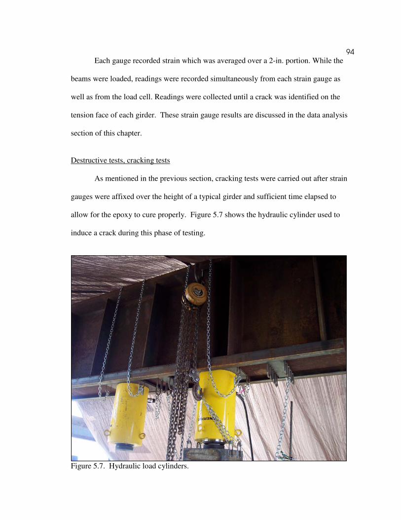
94

Each gauge recorded strain which was averaged over a 2-in. portion. While the

beams were loaded, readings were recorded simultaneously from each strain gauge as

well as from the load cell. Readings were collected until a crack was identified on the

tension face of each girder. These strain gauge results are discussed in the data analysis

section of this chapter.

Destructive tests, cracking tests

As mentioned in the previous section, cracking tests were carried out after strain

gauges were affixed over the height of a typical girder and sufficient time elapsed to

allow for the epoxy to cure properly. Figure 5.7 shows the hydraulic cylinder used to

induce a crack during this phase of testing.

Figure 5.7. Hydraulic load cylinders.

95

A single point load was applied at mid-span, to the compression face of each

girder. Each girder was loaded in 5,000-pound increments until a visible crack had

formed. An additional 10,000-pound load was applied beyond this point. The girder was

unloaded and loaded again until a minimum of three cracking tests were performed on

every girder. As such, all cracks could be properly identified and accounted for. Girders

were inspected in 10,000-pound increments up through an applied load of 60,000-pounds.

Beyond this point, each girder was inspected in 5,000-pound increments. A mirror was

oriented beneath each girder at mid-span to facilitate this process (Figure 5.8). The

applied load as well as corresponding strain readings and deflection readings were

recorded during this phase of testing. Results are discussed in the data analysis section.

Once the crack formed, the load was increased a nominal amount and kept

constant. Every crack that formed under the applied load was then traced with a

permanent marker. Typically, cracks were visually identified in the 95 to 105-kip range.

All cracks were in close proximity to the mid-span of each girder. Crack locations were

noted and used in determining the moments at the decompression loads.

Figure 5.8. Crack identification.

96

Destructive tests, decompression loads

Prior to conducting the decompression tests on a given girder, it was necessary to

affix a series of strain gauges on the tension face of the girder. These gauges were

oriented near the center-line of the beam and are pictured in Figure 5.9. Two ¼-in. strain

gauges were epoxied to either side of the crack. One 2-in. strain gauge was epoxied

directly over the crack. Each was affixed to the tension face of the girder and placed

under pressure while curing according to the manufacturer’s specifications.

As with the cracking tests, a single point load was once again applied at mid-span,

to the compression face of each girder. The load was applied in 5,000-pound increments

and a minimum of three cycles of decompression tests were conducted. Data collected

from each cycle was then averaged to determine decompression load for each girder.

Recall that the decompression load is by definition the load at which the instrumented

crack(s) open. The decompression load is determined in accordance with the procedures

outlined in Chapter 4. Each cycle was terminated after readings from the ¼-in. strain

gauges recorded a bi-linear response and the 2-in. strain gauge reached a conservative

threshold of 2,000 to 3,000 microstrain.

Figure 5.9 Strain gauges used to identify the decompression load.

97

The 3,000 microstrain threshold insured that the strain gauge could be re-used

from cycle to cycle without incurring any adverse effects. Computer software and a data

acquisition system were used to continuously record the strain and load throughout these

tests. This meant that data could be viewed in real-time which were an added advantage.

The ¼-in. strain gauges placed to either side of the crack are representative of the

standard procedure for determining the decompression load (Pessiki, Kaczinski, and

Wescott, 1996). The decompression load is used to calculate the effective prestress force.

For comparison, a single strain gauge was placed over the crack and data was collected in

unison with the strain gauges placed to either side of the crack. Data collected from both

techniques are the result of the cracking test which is a destructive test. This means that

once cracked, the effective prestress force in the girder can be determined. To test

girders in this manner means that a bridge must first be decommissioned, bridge girders

hauled to an off-site testing facility, and the residual prestress force is determined after

the fact. Results for the non-destructive tests are presented in the data analysis section of

this chapter.

Non destructive testing, saw cuts

As a viable alternative to the destructive testing, currently the commonly used

way to quantify the residual prestress force, this phase presents a non-destructive

procedure to directly quantifying such a value. In effect, this non-destructive approach

means that the residual prestress force is directly quantifiable and can be obtained from

in-service girders without any sustained damage.

98

Of the eight girders tested, two groups were created. For the first group, the

residual prestress force was first arrived at destructively and then subsequently non-

destructively. This order was reversed for the second group of girders. Since each girder

was tested in both a destructive and non-destructive fashion, pair wise comparisons could

be made. Also, one could address whether or not one type of test influenced the results

from the other type of test. As will be shown, the order of operations did not appear to

influence results from either test. Results are presented and discussed in the data analysis

section.

Each girder was subject to two sets of non-destructive tests. In turn, each set of

non-destructive tests consisted of one strain gauge (oriented through the length-wise

centerline on the tension face of each girder) and saw cuts were placed ¼ -inch to either

side of the strain gauge (Figure 5.10).

Figure 5.10. Non-destructive testing.

99

Each pair of saw cuts transverse the entire bottom flange of the beam. After

zeroing and calibrating each strain gauge, twelve pairs of saw cuts were made in

increasing increments of 1/8-in. in depth in between each strain gauge reading.

Accordingly, changes in strain were recorded with the data acquisition system up through

a depth of 1½-in. The cuts were not made deeper than 1½ in. due to the fact that the

bottom most row of prestressing strands in newly constructed girders is typically 2-in.

above the tension face. Typically, changes in strain were shown to diminish as the depth

of saw cuts approached 1½ –in. This trend was important for the following two reasons:

1) a safety margin of ½-inch could be provided for the majority of prestressed

girders that have been, are being, or will be constructed ;and,

2) as will be shown, the strain gauge readings taken at this depth resulted in a

residual prestress force that was comparable to the prestress force arrived at

through the destructive tests for the majority of girders tested.

Strain gauges that were 2 in. and 4-in. in length were used for this phase of the

research. The appropriateness of these gauge lengths will be addressed in the results

section. Of the two strain gauges used in conjunction with the non-destructive tests, each

was affixed 4 feet to either side of mid-span. To this end, strain gauge readings were

directly comparable to one another as the moment due to self-weight was equal at both

instrumented locations due to the girder preparation ( refer to the deck in Figures 5.1 and

5.2). Assuming that a uniform moment due to self weight can be achieved, any two

equidistant locations would have sufficed. This is true so long as the strain gauges were

not placed within 60 strand diameters from either end of a prestressed concrete girder

100

where the strand is still within the development length. Results are presented and

discussed in the Data Analysis section.

Data Analysis

Girder Properties

A major portion of the focus of this research is to determine the feasibility of

implementing a non-destructive approach for directly quantifying the residual prestress

force of an in-service bridge girder. The objective of each section is to present data as it

relates to that goal. Accordingly, in the data analysis section, two pertinent questions

must be answered:

1) Do the girder and deck act in a composite fashion?

2) How must the section properties be handled, gross, transformed, a combination

thereof?

The non-destructive test focuses on the strain on the tensile face of the girder. For a

prestressed concrete girder, the following figure represents the superposition of total

stress throughout the cross section (Figure 5.11).

Figure 5.11. Stress distribution in a prestressed girder.

101

As shown in Figure 5.11, the cross-section area (A), moment of inertia (I), the

centroid of the member (c) and the eccentricity (e) due to the prestressing force (P) are

parameters that affect the two questions posed at the beginning of this section. This

equation is as follows:

σ = -P – Pec + Mc (5.1) A I I This equation solves for stress at a particular location on the cross section. All

variables were defined in the previous paragraph except for the moment due to self

weight (M). Therefore the modulus of elasticity of both the deck and girder concrete

must be determined, assuming that the deck and girder behave in a composite fashion.

To answer this question attention was placed on determining the centroid of each

member. Strain gauges were placed at various heights on the member, and were analyzed

for three separate loads during the first cycle of the cracking tests. The loads analyzed

were: 25,000, 50,000, and 75,000 pounds. The corresponding strain gauge readings

associated with each of these loads were then plotted against their vertical elevation as

measured from the tensile face of the girder. This type of plot results is an intersection

point. This intersection point corresponds to the neutral axis of the girder. Assuming the

stresses remain in the elastic range, the intersection point passes through the centroid of

the section. All three load cases were below the cracking load and were taken from the

first cycle. As such, it was reasonable to assume that the incurred stresses did in fact

remain in the elastic range. In turn, this meant that the neutral axis and centroid were in

fact the same value. A typical strain versus elevation plot is shown below in Figure 5.12.

The neutral axis for Girder 7 was experimentally determined to be 18.5 in.

102

Beam 7 Neutral Axis

0

5

10

15

20

25

30

35

-150 -100 -50 0 50 100 150

micro strain

dis

t fr

om

bo

tom

(in

.)

25 K

50 K

75 K

Figure 5.12. Girder 7 neutral axis test.

To arrive at the transformed section properties, core samples were extracted

from concrete blocks at the conclusion of the field tests (Figure 5.13). Averaging the

results from these cores resulted in a modulus of elasticity of 5,660ksi for the girder and

3,650 ksi for the deck (Appendix A). Flexural capacity tests indicated that the deck and

girder were acting in a composite fashion, however the concrete pads placed atop each

girder were not acting in a composite fashion. This meant that only the girder and deck

would be included in calculations. Calculations, based on field measurements for Girder

7 are in close agreement to the measured values. A value of 18.2 inches was arrived at

when the gross area of the girder was used in conjunction with the transformed area of

the deck.

103

Values for the neutral axis that was experimentally determined from data

collected during the cracking tests and centroid that was based on hand calculations and

field measurements are presented in Figure 5.14. Values presented in Figure 5.14 indicate

that the measured neutral axes from all girders were in close agreement with the

calculated values when the gross area of the girder was used in conjunction with the

transformed area of the deck. All values were well within 10% of one another.

Figure 5.13. Saw-cutting a block from girder 4.

104

Figure 5.14. Neutral axes, measured and calculated.

Plots, similar to Figure 5.12, are included in Appendix B for each beam. As such,

both questions presented at the beginning of this section were answered as follows:

1) the girder and deck exhibited composite behavior whereas the pad did not; and,

2) field tests indicated that equations involving section properties would be

adequately handled when the gross cross-sectional properties were used for the

girder and transformed properties were used for the deck.

Results from the decompression tests and corresponding residual prestress forces are

presented in the Destructive Test Results section.

Destructive test results

Measured strain values recorded from the decompression tests were used to

determine the residual prestress force. Both the procedure and equations have already

been presented in Chapter 4. Therefore this section presents and addresses the results

Neutral Axis

0

5

10

15

20

25

G1 G2 G3 G4 G5 G6 G7 G8

Beam ID

Ne

utr

al A

xis

(in

.)

Measured

Calculated

105

from the destructive (cracking) and the non-destructive test taken to determine the

decompression load. Brief summaries for each of these approaches are as follows:

1) For the destructive test, once the girder has been cracked, strain gauges were

placed to either side of the crack (Figure 5.9). Data from these strain gauges

exhibit a bilinear behavior as the crack opens when the applied load was plotted

against the corresponding strain. Trend lines were fit to each linear portion of this

curve. These lines were then extended until they intersected. The applied load

corresponding to the point of intersection is taken as the decompression load.

This approach, developed by Pessiki, Kaczinski, and Wescott (1996), serves as

the standard to which the second approach is compared to.

2) The modified destructive approach allows for a single strain gauge to be placed

directly over the crack (Figure 5.9). Here measured strains gradually deviate from

a trendline that starts at the origin and passes through a linear series of points.

This trendline is then extended beyond the deviation point by a nominal amount.

The load associated with the point, just prior to deviation, is taken as the

decompression load.

Both techniques are shown to hold merit. There are situations where one technique may

be preferred over the other, especially if less interpretation is required using a particular

method. These situations will be discussed in greater detail at the end of this section.

Accordingly typical responses for each destructive gauge placement are presented in

Figure 5.15. Additional responses are included in Appendix C. These plots presented in

this figure are considered to be ideal.

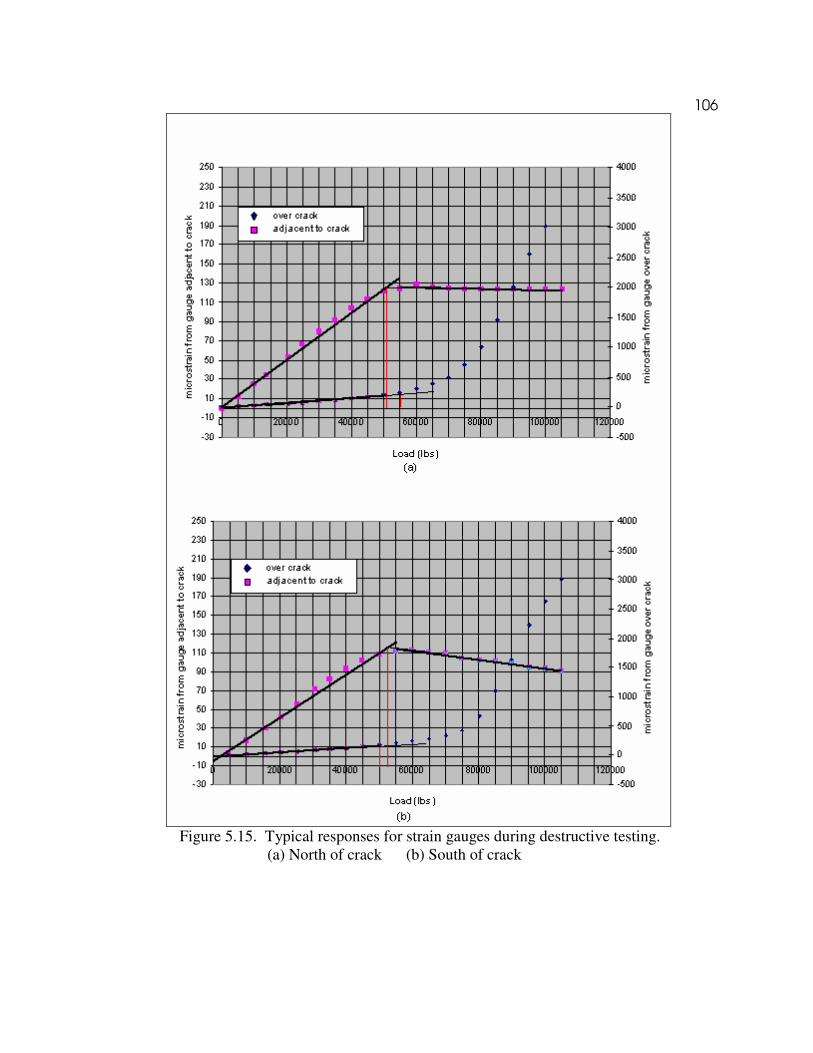
106

Figure 5.15. Typical responses for strain gauges during destructive testing. (a) North of crack (b) South of crack

107

The standard method (strain gauges on either side of crack) presented in

Figure 5.15 will be discussed first. For this method, refer to the strain readings on the

left-hand side of the plots in conjunction with the data set(s) that eventually plateau as

loading continues to increase. Two graphs are shown in Figure 5.15. Figure 5.15(a)

presents data collected from the ¼-in. strain gauge placed to the north of the crack and

monitored during the first cycle of the decompression test. Figure 5.15(b) presents data

collected from the ¼-in. strain gauge placed to the south of the same crack and monitored

during the second cycle of the decompression test. For both load cases, intersecting lines

were used to pinpoint the decompression load using the standard method. Plots for both

strain gauges and each cycle typically exhibited a bi-linear behavior for an increasing,

applied load. An increase in the applied load resulted in a linear increase in strain

readings until the point where the crack opened. Decompression loads of approximately

50,000 pounds and 51,250 pounds were noted from the respective gauges. This indicated

that the gauges and cycles behaved in a consistent and precise manner for the standard

method.

The modified method presented in Figure 5.15 (a) and (b) will now be discussed.

For this method, refer to the scale of strain readings on the right-hand side of the plots

and the data set(s) that climb at an increasing rate as a result of larger applied loads.

Again, two graphs are shown in Figure 5.15. Figure 5.15(a) presents data collected from

the 2-inch strain gauge placed directly over the crack during the first cycle of the

decompression test. Figure 5.15(b) presents data collected from the same strain gauge,

during the second cycle of the decompression test. In both instances, the decompression

load could be identified using the modified method. Plots for each girder and each cycle

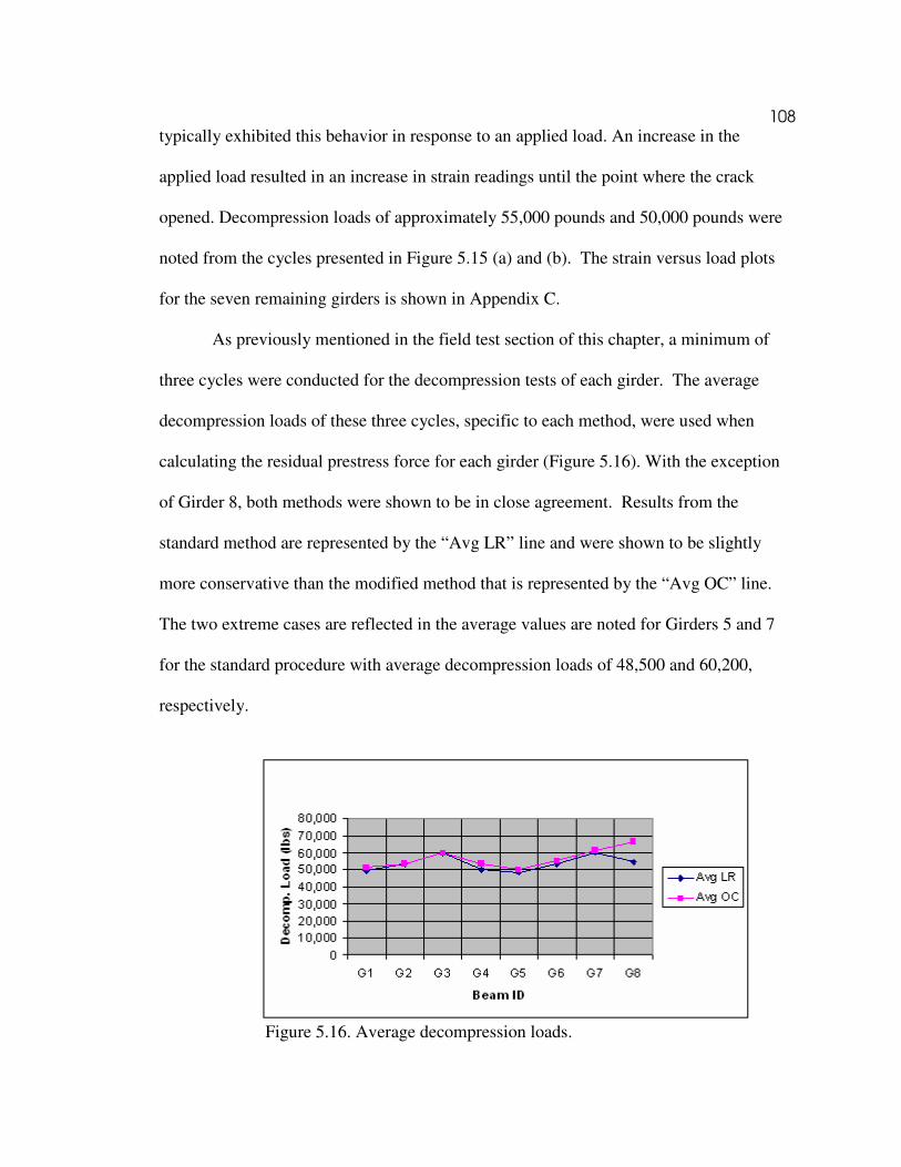
108

typically exhibited this behavior in response to an applied load. An increase in the

applied load resulted in an increase in strain readings until the point where the crack

opened. Decompression loads of approximately 55,000 pounds and 50,000 pounds were

noted from the cycles presented in Figure 5.15 (a) and (b). The strain versus load plots

for the seven remaining girders is shown in Appendix C.

As previously mentioned in the field test section of this chapter, a minimum of

three cycles were conducted for the decompression tests of each girder. The average

decompression loads of these three cycles, specific to each method, were used when

calculating the residual prestress force for each girder (Figure 5.16). With the exception

of Girder 8, both methods were shown to be in close agreement. Results from the

standard method are represented by the “Avg LR” line and were shown to be slightly

more conservative than the modified method that is represented by the “Avg OC” line.

The two extreme cases are reflected in the average values are noted for Girders 5 and 7

for the standard procedure with average decompression loads of 48,500 and 60,200,

respectively.

Figure 5.16. Average decompression loads.

109

For the modified method, the extreme cases were reflected in Girders 5 and 8

with average decompression loads of 50,000 and 66,700 pounds, respectively. Ratios of

the standard method to the modified method are summarized in Figure 5.17. As

previously mentioned, the standard method was predominantly shown to be conservative.

Aside from beam eight, the modified approach was shown to be in close agreement.

Reported percentages for the remaining seven girders ranged from 94% for Girder 4 to

101% for Girder 2.

Accordingly, for the two destructive methods, the more conservative results were

obtained with the standard method. Still, instances arise when a bilinear response is not

always exhibited in data collected from strain gauges placed to the left and right hand

side of a crack. In instances such as these, the modified approach could be used in lieu of

the standard approach where interpreting a bilinear response would clearly be subject to

greater interpretation. The modified method is within 4.5% of standard method.

Decompression Load Ratio

0.00

0.20

0.40

0.60

0.80

1.00

1.20

G1 G2 G3 G4 G5 G6 G7 G8

Beam ID

Rati

o

ratio (Avg LR/AvgOC)

Figure 5.17. Decompression load ratios.

110

The decompression load is a critical parameter that is used to determine

residual prestress force. Both the procedure and parameters for calculating the residual

prestress force were presented in Chapter 4. This residual prestress force is crucial

because ultimately, it is this force that is used in assessing the flexural capacity of a

girder. Decompression loads arrived at through both methodologies has been combined

with the appropriate measured parameters from each girder when calculating the residual

prestress force. To this end, the effects of employing the modified method can be

explored further by evaluating the values presented in Table 5.1.

The first column lists the ID while the second column lists values for the effective

prestress force when the standard method for determining the residual prestress force was

used. The third column represents the same parameter when the modified method is

used. As expected the extreme cases are again Girders 5 and 7 for the standard method

and Girders 5 and 8 for the modified method. It is more useful from a design prospective

to present the effective (or residual) prestress force in terms of a percentage of the jacking

stress. Recall from Chapter 2, that the jacking stress is the stress in the strands just prior

to destressing. Typically, this jacking stress is specified on plan-sheets. Such values

were not available on plan sheets provided for this particular bridge.

Table 5.1 Residual prestress force (Pe) Beam ID Pe based on Avg. LR (lbs) Pe based on Avg OC (lbs)

G1 191,240 197,160

G2 190,420 188,770

G3 200,920 202,180

G4 181,540 191,930

G5 178,570 183,700

G6 195,680 199,750

G7 219,210 224,340

G8 205,810 249,310

111

Despite this, the jacking stress can be arrived at through the strand type, and

diameter. For 7/16-in. diameter, 7-wire, 250 ksi strands a minimum, ultimate breaking

strength of 27,000-pounds per strand is the recognized standard for a girder fabricated in

Utah during this time period. Therefore according to the code a jacking stress that is 70%

of this value is permitted. Accordingly, the values presented in Table 5.1 are compared

against a combined jacking stress of 264,600 pounds as there were 14 strands in each of

the eight girders. A summary of these comparisons are presented for each girder in

Figure 5.18.

The percent losses reflect approximately 40 years of service for the eight

AASHTO Type II prestressed concrete bridge girders. Calculated losses were lower in

seven of the eight girders when the modified method was employed for determining the

decompression load. Smaller losses indicate larger residual prestress forces that result in

a less conservative approach. The percent loss for five of the eight girders ranged from

20 to 30% loss when either destructive method was used.

Figure 5.18. Percent loss of jacking stress.

Percent Loss of Prestress force

0.00

5.00

10.00

15.00

20.00

25.00

30.00

35.00

G1 G2 G3 G4 G5 G6 G7 G8

Beam ID

Pe

rce

nt

Lo

ss

(%

)

% Loss (Avg LR)

% Loss (Avg OC)

112

Prestress losses over time generally result in a reduction of initial

prestressing force between 10 to 30% (Collins and Mitchell, 1987). To put this

difference in the context of the residual prestress force per strand, approximately 13,950

lbs per strand remain when the standard method for determining the decompression load

is used. Similarly, 14,610 lbs per strand remain when the modified method is used to

determine the decompression load. The residual prestress force for the destructive and

non-destructive test results will be compared to each other as well as to specified and

analytical values in a subsequent section.

Assuming both methods are used together to determine the decompression load, it

would be safe to use the more conservative results. Depending on the shape of the

response curves generated, the method that is preferred may be the one that is subject to

the least amount of interpretation. Now assuming both of these conditions are met

through a single method, then the path is clear. If not, engineering judgment is required.

Non-destructive test results

The field tests section described how the non-destructive test was performed.

This section will present and discuss the results of the test. To put these results into some

sort of framework, a series of questions will be posed. Results pertaining to those

questions will then be presented and discussed. To this end, the following questions are

posed:

1) How does a strain reading taken at the bottom of a beam relate to residual

prestress force?

113

2) How do these strain readings compare to destructive, specified and analytical

values?

3) How were the parameters fixed for the non-destructive test (depth, width, length,

separation)?

4) Two sets of non-destructive tests were performed on each girder, how did they

compare to one another?

5) Two gauge lengths were used here, did one perform better than the other?

6) Four of the eight girders were first tested destructively, then non-destructively.

Did this have any affect on the test results?

7) Overall, were the saw cuts an effective method for determining the residual

prestress force?

Ultimately the non-destructive method must result in quantifiable prestress forces and be

performed on in-service members without imparting any permanent damage. The

questions proposed above will now be addressed.

Relating strain readings to residual prestress force. In answer to the first question

posed, strain is related to residual prestress force via equation 6 (presented earlier in this

chapter). As defined, this equation solves for the stress in the bottom of the member. We

are interested in the latter. Again, Equation 5.1 is again presented as follows:

σ = -P – Pec + Mc (5.1) A I I

All of the variables associated with this equation were defined previously. Armed

with the modulus of elasticity, the stress at the bottom of the girder can be solved for,

114

based on the corresponding strain gauge reading. As such the only unknown

becomes the residual prestress force, P. This variable can then be solved for directly.

Table 5.2 presents these variables and the resulting prestress force for Girder 5.

Table 5.2 lists all measured values including cross-sectional properties, the

modulus of elasticity for the prestressed concrete girder, and the eccentricity of the

prestressing steel. Also included is the moment due to self weight at the location where

the strain gauge is located. The variable “ε saw cuts @ 1.5 in deep” reflects the strain

reading at a specified depth for this particular strain gauge. At this point, the effective

prestress force can be solved for as all other variables are known. In the procedure

outlined in Table 5.2, Peff is solved for via interpolation. Alternatively, the effective

prestress force can be solved for using an iterative approach; the solution converges

relatively quickly. A solution is achieved when the right hand and left hand side of

Equation 5.1 equal one another. Both approaches yield the same answer.

Table 5.2 Solving for the effective prestress force

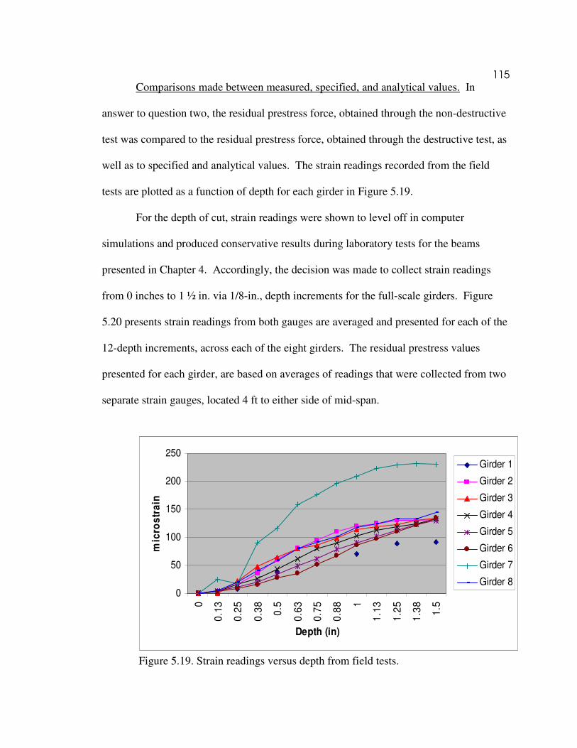
115

Comparisons made between measured, specified, and analytical values. In

answer to question two, the residual prestress force, obtained through the non-destructive

test was compared to the residual prestress force, obtained through the destructive test, as

well as to specified and analytical values. The strain readings recorded from the field

tests are plotted as a function of depth for each girder in Figure 5.19.

For the depth of cut, strain readings were shown to level off in computer

simulations and produced conservative results during laboratory tests for the beams

presented in Chapter 4. Accordingly, the decision was made to collect strain readings

from 0 inches to 1 ½ in. via 1/8-in., depth increments for the full-scale girders. Figure

5.20 presents strain readings from both gauges are averaged and presented for each of the

12-depth increments, across each of the eight girders. The residual prestress values

presented for each girder, are based on averages of readings that were collected from two

separate strain gauges, located 4 ft to either side of mid-span.

0

50

100

150

200

250

0

0.1

3

0.2

5

0.3

8

0.5

0.6

3

0.7

5

0.8

8 1

1.1

3

1.2

5

1.3

8

1.5

Depth (in)

mic

ros

tra

in

Girder 1

Girder 2

Girder 3

Girder 4

Girder 5

Girder 6

Girder 7

Girder 8

Figure 5.19. Strain readings versus depth from field tests.

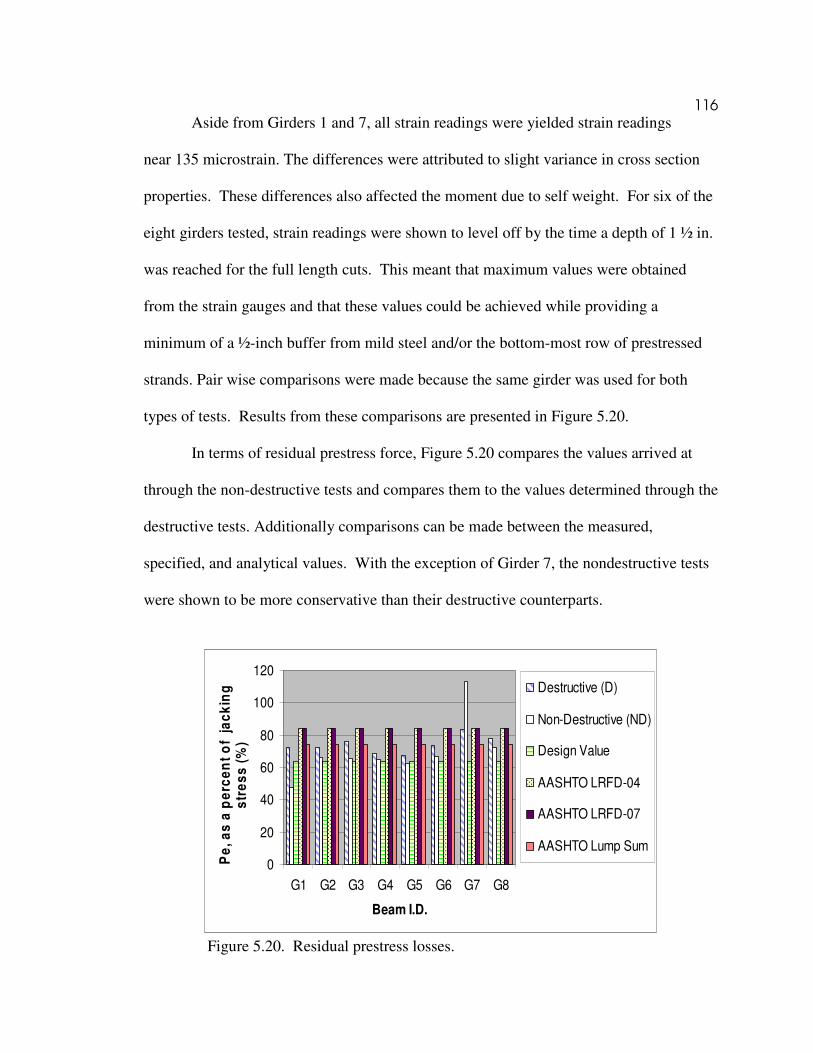
116

Aside from Girders 1 and 7, all strain readings were yielded strain readings

near 135 microstrain. The differences were attributed to slight variance in cross section

properties. These differences also affected the moment due to self weight. For six of the

eight girders tested, strain readings were shown to level off by the time a depth of 1 ½ in.

was reached for the full length cuts. This meant that maximum values were obtained

from the strain gauges and that these values could be achieved while providing a

minimum of a ½-inch buffer from mild steel and/or the bottom-most row of prestressed

strands. Pair wise comparisons were made because the same girder was used for both

types of tests. Results from these comparisons are presented in Figure 5.20.

In terms of residual prestress force, Figure 5.20 compares the values arrived at

through the non-destructive tests and compares them to the values determined through the

destructive tests. Additionally comparisons can be made between the measured,

specified, and analytical values. With the exception of Girder 7, the nondestructive tests

were shown to be more conservative than their destructive counterparts.

0

20

40

60

80

100

120

G1 G2 G3 G4 G5 G6 G7 G8

Beam I.D.

Pe

, a

s a

pe

rce

nt

of

ja

ck

ing

s

tre

ss

(%

)

Destructive (D)

Non-Destructive (ND)

Design Value

AASHTO LRFD-04

AASHTO LRFD-07

AASHTO Lump Sum

Figure 5.20. Residual prestress losses.

117

On average, the residual prestress force obtained from the non-destructive

tests was 94% of the destructive tests when directly determining residual prestress force.

Two outliers were noted for the non-destructive tests, namely Girders 1 and 8. The non-

destructive data is skewed slightly. If one removes these two outliers from this scenario

when comparing the results, the prestress force from the non-destructive tests are 92% of

the prestress force from the destructive test. However, because all tests were performed

in a concise and repeatable manner, the remaining comparisons will be based on all eight

girders.

On average, the non-destructive test results were 94% of the destructive test

results. This indicates that a margin of safety is accounted for when the non-destructive

technique is used. The design calculations specify an effective prestress force, hereafter

referred to as the design value that is 64% of the jacking stress (169,000 lbs). Compared

to the destructive test results, the design value underestimated the effective prestress

force by 16% on average. Compared to the non-destructive test results the design value

underestimated the effective prestress force by 9% on average.

Compressive strengths of 4 ksi (initial) and 5 ksi (28-day) were specified on the

plan sheets for the prestressed girders. A 28-day strength of 3-ksi was specified for the

deck. These compressive strengths were used for the analytical prediction methods. By

averaging the results presented in Figure 5.20, the AASHTO LRFD-04 method

overestimated the destructive results for residual prestress force by 12% on average.

Compared to the non-destructive test, this method overestimated the residual prestress

force by 17%, on average.

118

The AASHTO LRFD-07 code is based on transformed section properties.

Compared to the destructive tests results, this method over predicted the residual

prestress force by 11% on average. When compared to the non-destructive tests results,

this method over predicted the residual prestress force by 16% on average. Lastly, the

AASHTO Lump Sum method equaled the residual prestress force via the destructive tests

and overestimated the residual prestress force via the non-destructive tests by 6%, on

average.

Collectively, there was little difference in the net result between the AASHTO-

LRFD-07 and the AASHTO-LRFD-04 analytical methods. Both approaches are a

function of the jacking stress. The AASHTO Lump Sum method closely approximated

the measured values, when averages were compared.

As previously mentioned, the analytical approaches encompass the AASHTO

LRFD-07, the AASHTO LRFD-04, and the AASHTO Lump Sum methods were used for

estimating residual prestress loss. The procedures for each method are summarized

below.

The AASHTO LRFD-07 method is designed specifically to estimate prestress

losses in high-strength pretensioned concrete girder bridges. Advantages to this method

include better predictions of the modulus of elasticity, creep, and shrinkage of concrete

(Tadros et al., 2003). The equation used to estimate the modulus of elasticity via the

AASHTO LRFD-07 method was presented previously in Chapter 2. As such the

remaining equations, as defined by Tadros et al. (2003), are defined as follows:

∆fpES = ni (fcgp) (5.2)

119

This equation reflects the instantaneous prestress loss due to elastic shortening

at transfer. The variables for this equation are defined as follows: ∆fpES represents the

loss of steel stress due to elastic shortening (ksi); ni stands for the initial steel modular

ratio; and fcgp corresponds to the concrete stress at the center of the prestressing steel due

to the initial prestressing force. This variable, in turn is solved for in the next equation:

(5.3)

The variables represented in Equation 8 are defined next. The variables yet to be defined

follow: Ati denotes the area of the transformed section at transfer (in2); epti stands for the

eccentricity of steel with respect to the initial transformed section (in); Mg represents the

maximum moment due to self weight (k-in); Iti denotes the transformed moment of

inertia at transfer (in4).

The next set of equations represents long term losses between the time of the

prestressing force are transferred and the deck is placed for the AASHTO LRFD-07

method. Equation 9 solves for prestress loss due to shrinkage,∆fpSR (ksi), during this time

frame.

∆fpSR = εbid Ep Kid (5.4)

Here values for the following three variables are required to solve this equation. The

variables include: εbid which denotes shrinkage of the girder between transfer and deck

placement (in/in); Ep represents the modulus of elasticity of prestressing steel (ksi); and

Kid represents the transformed effective modulus of elasticity factor during the above-

mentioned timeframe.

120

The prestress loss due to creep, ∆fpCR (ksi), accounts for deformation under

an applied load between the times of transfer and deck-placement. This parameter is

presented in Equation 5.5.

∆fpCR = ni fcgp ψbid Kid (5.5)

The only variable yet to be defined is ψbid. This is a girder creep coefficient that is a ratio

of the strain that exists at deck placement to the elastic strain that due to the applied load

at transfer.

Relaxation, ∆fpR2 (ksi), as handled by the AASHTO LRFD-07 method is broken

into two time increments. The first increment of 1.2 ksi is accounted for prior to deck

placement. The other 1.2 ksi is accounted for after deck placement.

The final set of equations reflects long term losses from the time the deck is cast

through the final time via the AASHTO LRFD-07 method. Equation 11 solves for the

prestress loss due to shrinkage of girder concrete in the composite section, ∆fpSD (ksi),

during this time frame.

∆fpSD = εbdf Ep Kdf (5.6)

Here, εbdf represents shrinkage in the girder between deck placement and final time. The

variable Kdf represents the transformed effective modulus of elasticity factor during the

above-mentioned timeframe.

There are two equations presented for prestress losses due to creep. The first

equation reflects prestress loss due to creep of girder concrete in the composite section

caused by initial prestressing force and self weight based on the coefficients presented in

Equation 5.7.

121

∆fpCD1 = ni fcgp(ψbif-ψbid) Kdf (5.7)

Of these variables the only one yet to be defined is ψbif, this signifies the girder creep

coefficient that accounts for the ratio of strain at final time to the elastic strain incurred at

the time of transfer. The fact that this coefficient is based in part on time final is the

reason it is presented here.

The second equation that accounts for prestress loss due to creep of girder

concrete in the composite section is termed ∆fpCD2 (ksi); this variable is based on creep

that is caused by deck and superimposed dead loads. This long-term prestress loss

component is presented in Equation 5.8.

∆fpCD2 = n fcdp ψbdf Kdf (5.8)

The variable n denotes the steel modular ratio; namely, the modulus of the prestressing

steel divided by the modulus of the concrete. The next variable, fcdp, represents the

concrete stress at the center of the prestressing steel due to the deck and superimposed

loads. The ratio of strain which exists at final time to the elastic strain caused when load

is applied at the time of deck placement is symbolized by ψbdf. The variable Kdf was

previously defined.

The final equation utilized by the AASHTO LRFD-07 method to predict prestress

losses is reflected in Equation 5.9; the prestress gain due to shrinkage of deck in the

composite section, ∆fpSS (ksi).

∆fpSS = ∆fssp Kdf n [1+X(ψbdf)] (5.9)

122

Where ∆fssp stands for the change in concrete stress are the level of prestressing

strands due to shrinkage in the deck and X signifies an aging coefficient. This coefficient

accounts for concrete stress variability with time and is taken as a constant (0.7).

The second method employed to predict prestress losses is the AASHTOLRFD-

04 method. Here the elastic shortening loss due to the prestress force and self weight of

the girder are calculated using the following equations.

(5.10)

Equation 5.10 represents the elastic shortening loss due to the initial prestress force,

∆fpES, at the instant the strands are cut is calculated using the initial stress (fpi) and the

cross section area (Aps) of the prestressing strands the cross section area of the

prestressing strands. The remaining variables associated with this equation are the cross-

sectional area of the beam (Abm), the moment of inertia of the beam (Ibm), and distances

from the bottom of the beam to the centroid (yb) and to the centroid of the prestressing

steel (ypb).

The elastic shortening loss due to the self weight of the girder, ∆fpESsw,

is reflected in Equation 5.11.

(5.11)

With the exception of the maximum moment due to the self-weight of the girder, Msw, the

remaining variables in this equation were defined in Equation 15. Associated units for

both equations are in ksi. The negative sign indicates that this is a loss in prestress loss,

or rather, a gain in prestress. This is a result of the prestressing tendons elongating under

123

a load. The same can be said for Equation 5.12, the elastic shortening “gain” due to

the deck.

(5.12)

As before the negative sign indicates that this is a loss in prestress loss, or rather, a gain

in prestress which is a result of the prestressing tendons elongating under a load. In this

instance it is due to the casting of the deck.

Similarly, Equation 5.13 constitutes the gain due to the superimposed loads.

(5.13)

Here, Msi represents the moment due to the super-imposed loads. The variable yc stands

for this distance from the bottom of the beam to the centroid of the composite section. In

keeping with this subscript, Ic denotes the composite moment of inertia. When total

losses are sought, the results from equations 5.10 through 5.13 are added together.

The remaining equations reflected in the AASHTO LRFD-04 method account for

prestress losses due to shrinkage, creep, and strand relaxation. For prestressed members

the loss in prestressing steel stress due to shrinkage, ∆fpSR (ksi), is presented in Equation

5.14.

∆fpSR = 17.0 - 0.150H (5.14)

Here, the average annual ambient mean relative humidity, H, is expressed as a percent.

Losses attributed to creep in the concrete, ∆fpCR (ksi), are shown in Equation 5.15.

∆fpCR = 12.0fcgp – 7.0∆fcdp (5.15)

124

The concrete stress at the center of gravity of prestressing steel at transfer is

represented by the variable fcgp; associated units are in ksi. The change in concrete stress

at the centroid of the prestressing steel due to permanent loads (less loads present at the

time the prestressing force was imposed) is symbolized by ∆fcdp (ksi).

The prestress losses due to relaxation of the prestressing strands, ∆fpR2 (ksi), are

estimated via the AASHTO LRFD-04 method with Equation 5.16.

∆fpR2 = 20 – 0.4∆fpES – 0.2(∆fpSR + ∆fpCR) (5.16)

All variables were defined previously.

The third analytical method employed for this portion of the research is termed

the AASHTO Lump Sum Method. It typically results in a more conservative prestress

loss estimate as a result of the closed for solution. This method is addressed in the

AASHTO LRFD Bridge Design Specifications Manual (2004). For 250 ksi prestressing

strand, Equation 5.17 is used to predict total prestress losses, ∆fpTotal.

(5.17)

The compressive strength of concrete is represented by f’c. The second variable, PPR,

stands for the partial prestress ratio. This ratio is presented next in Equation 5.18.

(5.18)

The cross-sectional area of the mild steel corresponds to As (in.2). Similarly, the cross-

sectional area of the prestressing steel corresponds to Aps (in.2). The yield strength of the

prestressing steel and the yield strength of the mild steel are symbolized by fpy and fy,

respectively; associated units are in ksi.

125

Non-destructive parameters

Attention will now be turned to determining the parameters associated with the

non-destructive test. The results presented for the non-destructive tests are based on saw

cuts placed ¼ inch to either side of the strain gauge. These cuts ran the entire width of the

girder and progressed in depth from 0 inches to 1½ inches in ½-in. increments.

First, these parameters were explored through a parametric study presented in

chapter 4. Highlighting the key points of that study, we saw that the modeled behavior

and beam theory were in agreement (Figure 4.11). Hand calculations were based on the

equation presented in Equation 5.1. Strain readings most closely approximated hand

calculations when a target combination was reached. Beyond this target combination, we

saw that for both the depth and length of cuts, associated strain readings increased by a

nominal amount and then leveled off (Figures 4.17 and 4.18). The width of cut barred no

significance, however the placement of these cuts, termed separation, in relation to strain

gauge did.

Laboratory tests indicated that full-length cuts placed ¼-inch to either side of the

strain gauge yielded strain readings that were still considered to be conservative.

Accordingly, full length cuts were preferred for such reasons as repeatability, precision

and accuracy in the field (Figure 5.21). As anticipated all strain readings were shown to

level off by the time a depth of 1 ½ in. was reached for the full length cuts. Aside from

girders 1 and 7, the results were tightly grouped. This was encouraging for two reasons.

It meant that the maximum values were obtained from the strain gauges and that these

values could be achieved while providing a minimum of a ½-in. buffer from mild steel

and/or the bottom-most row of prestressed strands.

126

-50

0

50

100

150

200

250

0

0.1

3

0.2

5

0.3

8

0.5

0.6

3

0.7

5

0.8

8 1

1.1

3

1.2

5

1.3

8

1.5

Depth (in)

mic

rostr

ain

Girder 1

Girder 2

Girder 3

Girder 4

Girder 5

Girder 6

Girder 7

Girder 8

Figure 5.21. Depth of cut versus average strain readings.

As such full length cuts that transverse the entire width of the bottom flange,

placed ¼ inch to either side of the strain gauge, should be made in 1/8-in. increments up

through but not exceeding 1 ½ inches in depth. The 1/8- in. increments are still advisable

to insure the circular saw is not overworked. Additionally, strain gauge readings

collected in these increments will indicate whether or not maximum values obtained, as

well as insuring that the gauges were functioning properly.

North and south strain gauges

Recall that two sets of non-destructive tests were performed on each girder.

These gauges were located equal distances away from the mid-span. The saw cuts, placed

to either side of these gauges, were performed in the same manner at uniform depths. For

any given girder, it was typical that one gauge reading overestimated the target value and

the other strain gauge underestimated the target value. If results from individual gauges

had been used, in lieu of reporting an average between these values, a closer

approximation of the destructive test results could have been achieved. However, the

127

depth at which the target values were achieved would vary anywhere between 1 and 1

½ in. In consequence, results from one opposing strain gauge would be omitted altogether

and the strain readings may not be maximized which would lead one to question the

validity of such a test. Without the results obtained through destructive tests there would

be little indication into the correct depth to use. In effect, this would pose quite a

problem. To emphasize this point, data results from the “north” and “south” strain gauges

are presented for Beam 8 in Figure 5.22. These results should be compared to a target

value of 156 microstrain, specific to Beam 8 section properties and destructive test

results. This is why subjectivity is all but eliminated, and repeatability is insured when

average strain readings are used for a pair of gauges (Figure 5.21). As was shown in

seven of the eight girders tested, averaging results from a pair of gauges for each girder,

allows for a consistent depth of 1 ½ in. to be used, and yields results that perform better

than values indicated on the design sheets, yet are still conservative when compared to

results obtained through the destructive tests. Both the average and target strain values

are presented in Table 5.2 of the next section.

Figure 5.22. Non-destructive test results for girder 8.

128

Gauge lengths

Next, recall that two gauge lengths were used here, a 2-inch strain gauge and a 4-

in strain gauge. More specifically, the strain gauges were assigned to each beam as

defined in Table 5.3. This table displays the girder I.D., the types of strain gauges

employed, individual values, average values, and a ratio of average values to target

values.

Upon examining the data presented in this table we see that the outlying non-

destructive tests came from a pair of 2-in. strain gauges associated with Girder 1, and a 4-

in. and 2-in. strain gauge associated with Girder 7. Eliminating these outliers we now

have two girders per group for comparison. By averaging the ratios for each group we

see that the 2-in. gauges, 4-in. gauges, and any combination thereof would suffice for

non-destructive purposes. This is promising when one considers the fact that both gauge

lengths are specified for concrete. If cost is an issue, the cheaper gauges, or rather the 2-

in. gauges, may prove to be a better option. Lastly, recall that four of the eight girders

were first tested destructively, then non-destructively. To assess whether or not this had

any affect on the test results we will then turn our attention to Table 5.4.

Table 5.3. Gauge length and corresponding strain readings

Beam I.D. North South

North Strain

South Strain

Avg. Strain

Target Strain Avg/Target

G1 2 in 2 in 105 79 92 145 0.64

G2 2 in 2 in 156 107 131.5 145 0.91

G8 2 in 2 in 171 118 144.5 156 0.93

G3 4 in 2 in 111 157 134 158 0.85

G4 4 in 2 in 168 98 133 141 0.95

G7 4 in 2 in 183 277 230 166 1.38

G5 4 in 4 in 135 124 129.5 140 0.92

G6 4 in 4 in 168 100 134 149 0.90

129

Table 5.4. Destructive and non-destructive results

Beam I.D.

Group

Avg. Strain

Target Strain Avg/Target

G1 D. First, N.D. Second 92 145 0.64

G4 D. First, N.D. Second 133 141 0.95

G6 D. First, N.D. Second 134 149 0.90

G7 D. First, N.D. Second 230 166 1.38

G2 N.D. First, D. Second 131.5 145 0.91

G3 N.D. First, D. Second 134 158 0.85

G5 N.D. First, D. Second 129.5 140 0.92

G8 N.D. First, D. Second 144.5 156 0.93

Order of operations

Table 5.4 can be used to assess this because the average strain readings are

representative of the non-destructive tests, namely the saw cuts at 1 ½ in. deep, and the

target strain are based on results obtained through the destructive tests. Girders 1, 4, 6,

and 7 first tested in a destructive fashion. Girders 2, 3, 5, and 8 were first tested in a non-

destructive fashion. We see from the first collection of girders that both outliers reside in

the destructive group. Closer inspection reveals that one outlier is a maximum, the other

is a minimum. Accordingly, a definitive statement can’t be made with regards to the

order that the tests were conducted and the fact that both outliers reside in this group.

Eliminating the outliers from the destructive group creates a mismatch. Keeping

all four girders in this group skews the data. As such eliminating outliers from both

groups seems appropriate for this comparison. In so doing the non destructive results

were both within 1% of one another and both were within 10% of target values. This

indicates that the order in which the destructive and non-destructive tests were conducted

did not factor into the performance of either set of results. Qualitatively speaking, results

that will be presented in the next chapter indicate consistent flexural capacities amongst

130

the girders. This indicates the nondestructive tests didn’t affect the destructive test

results. Overall, the saw cuts were an effective method for determining the residual

prestress force.

Conclusions

This portion of the research presents a series of destructive and non-destructive

tests used to evaluate the residual prestress force in a precast, prestressed concrete girder.

Eight AASHTO Type II bridge girders were salvaged from a bridge that had been in

service since the mid 1960s. These girders were 34.5 feet in length, prestressed with 14,

7/16 diameter prestressing strands. Plan sheets indicate that after losses a residual

prestress force of 169,000 pounds was designed for.

Girder properties

Results from the neutral axis field data, and hand calculations indicate that gross

properties should be used for the girders, and transformed section properties should be

used for the deck when determining the residual prestress force.

Destructive tests

Results indicate that for the two destructive methods employed to determine the

residual prestress force, the more conservative results would be evidenced through the

standard method. Instances may arise where a bilinear response is not always exhibited

in data collected from the standard approach. Here, the modified approach could be used

in lieu of the standard approach.

131

Non-destructive tests

Strain readings taken at the bottom of a beam directly relate to residual prestress

force. Field tests indicated that full-length cuts placed ¼-in. to either side of the strain

gauge yielded strain readings that were still considered to be conservative when made to

depths of 1 ½ in. For the depth of cut, strain readings were shown to level off as the

depth of cut approach 1 ½ in. On average, the non-destructive tests are 94% of the

destructive tests when directly determining residual prestress force.

Comparisons were also made between the measured values, the analytical values,

and the specified values. Based on the destructive test results, the specified value over-

estimated prestress losses by 16% on average. Compared to the non-destructive test

results the specified values were overestimated prestress losses by 9% on average. The

AASHTO LRFD-04/07 methods underestimated the prestress losses by 12% on average.

When compared to the non-destructive tests results, this method underestimated the

prestress losses by 17% on average. Lastly, the AASHTO Lump Sum method equaled the

destructive tests and over predicted the nondestructive tests by 6% on average.

132

CHAPTER 6

FLEXURAL CAPACITY AND DEFLECTION OF PRESSTRESSED

CONCRETE BRIDGE GIRDERS

Introduction

This portion of the research presents the flexural capacity and deflection

determined from field tests. Accurate prediction of the flexural capacity and associated

deflections under load are of great importance in the field of bridge engineering. As such

code based prediction methods continue to be refined as new information becomes

available. This is evidenced in the works of Seguriant, Brice, and Khaleghi (2005);

Labia, Saiid, and Douglas (1997); Hasley and Miller (1996); and Shenoy and Frantz

(1991). The measured flexural capacity is then compared to code estimates provided in

the AASHTO LRFD-04, AASHTO Standard Specifications-02, and the Prestressed

Concrete Institute Bridge Design Manual method, or rather the PCI-BDM-97 method.

When the deck and girder act compositely, the PCI-BDM-97 provides an iterative

solution that accounts for the compressive strengths of both sections. Seguriant, Brice,

and Khaleghi (2005) made mention of the fact that predicted values calculated using the

AASHTO LRFD-04 and AASHTO Standard Specifications, hereafter referred to as the

LRFD and Standard methods, are most representative of members of uniform

compressive strength. He goes on to say that both the LRFD and Standard methods can

still be used on composite members, but suggests that the results may be over-

conservative. All three codes are discussed in greater detail in a subsequent section.

133

Load and associated deflection readings are also presented in this chapter.

Here, field data is presented alongside of predicted values for deflection. For predicted

values, a computer program cited in Collins and Mitchell (1997), RESPONSE (TM

Borland) is used to generate a moment curvature diagram. The program, RESPONSE,

can be used to determine the load-deformation response of a prestressed concrete section

and helps develop an understanding of the response of prestressed concrete (Collins and

Mitchell, 1997). This program incorporates moment-area concepts that are based on

measured material properties and will be discussed in greater detail in a subsequent

section.

Field Tests

Flexural capacity and deflection

Testing for flexural capacity was the last field test performed for each of the eight

AASHTO Type II Girders. To vary the test scenarios, three point and four point loading

schemes were assigned to the salvaged bridge girders (Figure 6.1).

For all eight girders, the distance between the centers of the support beams was

272 inches. Because the girder’s overall length was 34 ½ feet, this left 71 inches of

overhang from the center of the support beams on either side. For the three point loading

scheme, a hydraulic cylinder was positioned at the mid-span of the beam. This midspan

location was 136 inches from the center of either support. Girders 1 and 2 were loaded to

failure in this manner. The remaining six girders were loaded to failure with an applied

constant moment region that varied from 2 to 9 feet. Girders 3 and 7 were failed with

applied constant moment distance of 2 feet. Girders 4 and 5 were failed with an applied

134

constant moment region of 6-feet. Lastly, Girders 6 and 8 were failed with an applied

constant moment region of 9-feet. The applied constant moment regions were centered

about the mid-span of each girder.

As with the cracking tests and decompression tests, the load was applied in 5,000

pound increments. The only difference here is that loading was applied through failure.

Deflection readings were collected with a 15-in. displacement transducer, capable of

collecting reading to the nearest 0.001 inches. The displacement transducer is pictured in

the foreground of Figure 6.2.

Figure 6.1. Three-point and four-point load cases.

135

Figure 6.2. The displacement transducer.

Prior to the start of each test the displacement transducer was “zeroed” and a field

check was performed to verify that the available stroke from the displacement transducer

corresponded to the measured distance. A couple of instances arose where the field

check and the displayed reading were not in agreement. In both instances it was the

result of a loose wire. This problem was easily addressed, and because it was caught

prior to testing, the test results were not affected. Prior to the start of each test, the

displacement transducer was adjusted for plumbness to insure accurate readings were

being recorded.

Flexural capacity, predicted values

Prior to presenting and discussing the results from the experimental tests, the

calculated code estimated values used for predicting flexural capacity will first be

discussed in greater detail. As mentioned in the introduction, three procedures were used

in estimating the flexural capacity; they were the AASHTO LRFD method, the AASHTO

Standard method and the PCI-BDM Method. Each will be discussed in the order that

they were introduced.

136

The AASHTO LRFD method. The following equations were used for

predicting the flexural capacity of a member using the LRFD method:

(6.1)

Where:

(6.2)

The variables “fps” and “fpu” denote the stress in the prestressing steel at the

nominal moment capacity and the ultimate tensile strength of the prestressing steel. The

variable “fpy” presented in Equation 6.2 represents the yield stress of the prestressing

steel. The steel used in the fabrication of the eight AASHTO type II girders was 7-strand

250 ksi that was 7/16-inches in diameter. Accordingly, these variables are 250 ksi for

“fpu” and 213 ksi for “fpy”. The variables “c” and “dp” are defined as the distance from

the extreme compression fiber to the neutral axis and the distance from the extreme

compression fiber to the centroid of the prestressing tendons, respectively. The variable

“c” is solved for based on equilibrium as follows:

(6.3)

Here “Aps”, “As”, and “As’” represent: the total cross-sectional areas of: the

prestressing steel, the mild reinforcing tensile steel, and the mild reinforcing compression

steel. Tensile tests on the actual mild reinforcement revealed that the yield stress of the

#5 bars used for both the compression and tensile steel was 60 ksi. Next “b” and “bw”

represent the width of the deck and width of the girder. The variable “β1” is the depth of

137

the whitney stress block compression zone. Lastly, the variable “hf” is the thickness

of the deck. All other variables were previously defined. Before the equation used to

predict the ultimate flexural capacity is presented it will be helpful to refer to Figure 6.3,

taken from Seguriant, Brice, and Khaleghi (2005).

Note that the ultimate flexural capacity is based on taking moments about a point

on the cross section. Figure 6.3 shows a model representative of the LRFD method. The

most notable attribute of Figure 6.3 is the fact that compression zones acting in the flange

overhangs are reduced by the factor β1. The ultimate moment capacity is now presented

as follows:

(6.4)

For the tested girders, “bw” and “b” were within a fraction of an inch from one

another of those girders tested in the field. Additionally, when calculating the flexural

capacity with the LRFD method, in accordance with Figure 6.3, the deck width, and the

web width are used for calculations; whereas the width of the top flange is omitted.

Figure 6.3. The AASHTO LRFD model.

138

Data presented in the results section will show that where “c” and “a” was

within the width of the flange, calculations involving “bw” utilized the top flange’s width.

Depending on the assumptions made, this wasn’t always the case. For situations where

“c” and “a” extended into the web, “bw” denoted the web width instead.

The AASHTO Standard method. Next we will turn our attention to the second

method used in predicting the flexural capacity, namely the AASHTO Standard method.

The main difference between the LRFD method and the Standard method according to

Seguriant, Brice and Khaleghi (2005) is that the factor “β1” is omitted from the model’s

treatment of the flange overhangs (Figure 6.4). For the tested girders, the width of the

deck-overhang and top flange were within a fraction of an inch. As such differences

between the Standard method and LRFD method were minimized. Had there been a

larger difference between the deck overhang and the top flange of the bridge girder,

differences between the two codes procedures would become much more apparent. The

β1 value was not the only difference between the code procedures. Their treatment of fps

varied as well.

Figure 6.4. The AASHTO Standard model.

139

The value of fps arrived at through method was typically higher than fps

arrived at through the LRFD method (Seguriant, Brice, and Khaleghi, 2005). In any

event, the overall goal here was to compare the code predictions to actual field capacities,

not to in-service capacities. Accordingly, “b” reflected the deck widths of the girders at

the time of testing, not the composite width while in service. The following equations are

representative of the Standard method:

(6.5)

(6.6)

Here, (6.7)

The variables associated with each of these equations were previously defined.

The PCI-BDM method. The most notable difference between the PCI-BDM

method and the previous two methods are the treatment of “β1”, and the fact that the

procedure is iterative in nature, rather than closed form. While this series of equations is

more involved, the result is that a weighted average of “β1” can be used, as opposed to

assuming a conservative value of “β1” typically associated with f’c of the deck. As

implied through the treatment of “β1”, this approach more readily lends itself to

predicting the flexural capacity of composite members which is typically the case for

bridge girders. To allow for direct comparison amongst each of the codes as well as to

field tests, the resistance factor, “Ф”, commonly associated with “Mn” has been omitted.

The model for the PCI-BDM method is presented next in Figure 6.5.

140

Figure 6.5. The PCI-BDM model. Conceptually speaking, the procedure presented in Figure 6.5 is solved when the

summation of the compression forces are equal in sign and opposite in magnitude to the

summation of the forces in the steel. The depth of “c” varies. In consequence, “β1” and

“a” also vary. The PCI-BDM equations, used to predict the flexural capacity, are

presented next. Upon assuming an initial value for “c”, solve the following equations.

(6.8)

Here “fpe” represents the effective prestress force during service. The effective

prestress force and the residual prestress force can be used interchangeably. Each

represents the prestress force once all losses have been incurred at some nominal point in

time. In Chapter 5, significant effort was dedicated to obtaining this parameter. Both

destructive and non-destructive techniques were used to directly determine this capacity.

In addition to the measured value, a design value for the effective prestress force was also

specified on the plan sheets. As such, all three values of effective prestress force were

applied to the codes. This will be addressed in the results section. The variable, “Ep”,

141

represents the modulus of elasticity of the prestressing strands; it was taken to be

28,500 ksi.

For non-tensioned reinforcing bars, the following equation was used to estimate

tensile strain:

(6.9)

Here, “di” denotes the depth of a particular steel layer from the extreme

compression fiber. Next, “fse” stands for the effective prestress. According to the PCI-

BDM, for non-tensioned reinforcement fse is -25,000 psi. An iterative approach was

used to solve for fps using the PCI-BDM method. Here, the following equation was used

in accordance with Table 2.11-1 of the PCI Bridge design manual for 250 ksi steel:

For εps ≤ 0.0076: fps = 28,500 εps (6.10)

For εps ≤ 0.0076: fps = 250 – 0.04/( εps – 0.0064) (6.11)

Both mild steel and prestressed steel were incorporated. As such the force in the

steel was determined by the following equation:

∑Asifsi = Apsfps + Asfs + As’fs’ (6.12)

The variables fs and fs’, refer to the stress in the mild steel, or rather the tension steel and

compression steel. Values associated with the compression zone are considered to be

negative. Values associated with tension steel are considered to be positive. Because fs

and fs’ are dependent on equation 6.9, each will differ in sign and magnitude.

In cases where the deck and girder have different compressive strengths, the depth

of the equivalent stress block, “a” is typically solved for as follows:

142

a = β1(avg) c (6.13)

where:

(6.14)

Initially, a value for β1(avg) must be chosen, then “a” can be calculated. This

procedure is repeated until β1(avg) converges using the subsequent values of “a” that result

from this trial and error process. Once a final value of β1(avg) is reached the compression

forces can then be calculated as follows:

∑Fcj = 0.85f'c[hf b]+0.85f'c[a-hf]bw (6.15)

All variables for Equation 6.15 were previously defined. Through the iterative

process of equating the compression forces to the force in the steel, one eventually arrives

at a point of equilibrium. At this point the corresponding values can be used to solve for

the flexural capacity as follows:

Mn = ∑Asi Fsi di + ∑Fcjdj (6.16)

Results from the field values and code estimate will be presented and discussed next.

Data Analysis

Flexural capacity

This portion of research addresses the implications of using theoretical as well as

field derived values. More specifically, the effective prestress force used in predicting the

flexural capacity of the eight AASHTO Type II bridge girders will be examined. These

girders were salvaged from a reconstruction project near Salt Lake City, Utah after 40-

143

plus years of service. There were additional reasons for the study. Where flexural

capacity is concerned seven scenarios were investigated. Both the scenarios and the

assumptions behind those scenarios are presented as follows:

Scenario 1: Under ideal circumstances, what is the absolute best that each code

can be expected to perform when compared to the flexural capacity tests? To

answer this question, the following scenario, thought to be the gold standard, is

presented. It is considered to be the gold standard in that the concrete strength of

both the deck and girder are known, actual section properties specific to each

girder are incorporated, and the effective prestress force based on the standard

destructive approach is used for each girder. As such, the code estimates are

girder specific.

Scenario 2: Scenario 1 is ideal but not totally realistic in that a destructive test

was used to determine the effective prestress force. Since the test was

“destructive,” the girder(s) would have had been taken out of service. In turn, this

would mean that the bridge is most likely no longer in service. Accordingly,

scenario 2 poses the following question, “How well would the codes perform if

results from the non-destructive tests were used in lieu of the destructive tests

used to directly determine the flexural capacity of each girder?” For this scenario,

the concrete strength of both the deck and girder are known, actual section

properties specific to each girder are incorporated, and the effective prestress

force based on the proposed non-destructive approach are used for each girder.

Here, the code estimates are girder specific.

144

Scenario 3: The first two situations present code estimates specific to each

girder. Typically, the more field data that one collects the better. But does data

specific to each girder mean that the codes must be run for each and every girder,

or rather can an average of the various parameters be used in conjunction with a

single run of the code(s)? For this scenario, the concrete strength of both the deck

and girder are known, average values based on actual section properties are

incorporated, and the average effective prestress force based on the proposed non-

destructive approach is used. Here, only one run through the code estimates is

required.

Scenarios 4 through 7 explore the implications of selecting theoretical values over

field values, and various combinations thereof, when estimating the ultimate flexural

capacity. To this end, when time is limited, or budgets are tight, what is the most vital

piece of information one should obtain? Accordingly, Scenarios 4 through 7 address this

question as follows:

Scenario 4: For this scenario, theoretical values specified on the plan sheets are used

for the concrete strength of both the deck and girder, theoretical section properties

are used, and the average effective prestress force based on the proposed non-

destructive approach is used. Here, only one run through the code estimates is

required.

Scenario 5: For this scenario, the concrete strength of both the deck and girder are

known, theoretical section properties are used, and the theoretical prestress force

that is specified on the plan sheets is used. Here, only one run through the code

estimates is required.

145

Scenario 6: For this scenario, theoretical values specified on the plan sheets are

used for the concrete strength of both the deck and girder, average values based on

actual section properties are incorporated, and the theoretical prestress force that is

specified on the plan sheets is used. Here, only one run through the code estimates is

required.

Scenario 7: For this scenario, theoretical values specified on the plan sheets are used

for the concrete strength of both the deck and girder, theoretical section properties

are used, and the theoretical prestress force that is specified on the plan sheets is

used. Here, only one run through the code estimates is required.

Findings, relevant to the questions posed in the above mentioned scenarios will now be

presented and discussed. As was mentioned in Scenario 1, field data was used in

conjunction with each prediction method. Results for Scenario 1 are shown in Figure 6.6.

0.0100.0200.0300.0400.0500.0600.0700.0800.0900.0

1000.01100.01200.01300.01400.0

Beam

1

Beam

2

Beam

3

Beam

4

Beam

5

Beam

6

Beam

7

Beam

8

Fle

xu

ral

ca

pa

cit

y (

kip

-ft)

LRFD Mn

STD Mn

PCI

Measured

Figure 6.6. Scenario 1: code estimates and measured values of flexural capacity.

146

The LRFD and Standard methods differed by less than 1 percent. Average

flexural capacities of 958 and 959 kip-feet were noted for the LRFD and Standard

methods. Although not clearly evident from the graph, slightly higher values were noted

for the Standard method when compared to the LRFD method. This result is based on

how the two codes treat the deck height and the calculation of fps. In either instance the

Standard method yielded higher values. Larger differences would most likely have been

noted had the deck widths been larger. However, increased deck widths would have

impeded the study due to clearance issues as well as capacity issues.

The PCI-BDM method was consistently shown to more accurately predict the

measured flexural capacity for each girder. This is attributed to the fact that the

compressive strengths of both the deck and girder are incorporated into the compressive

stress block. An average flexural capacity of 1014 kip-feet was achieved with the PCI-

BDM method. These averages can be compared against an average measured flexural

capacity of 1149 kip-feet.

Comparing these averages, percentage-wise, the LRFD and Standard codes were

84% of measured values and the PCI-BDM was 89% of the measured values. All code

estimates were shown to be conservative, individually and on average. Typically

resistance factors would be applied to values of Mn. Resistance factors were omitted

from this study. Had they been incorporated, greater separation between the predicted

values and measured values of flexural capacity may have been observed.

The measured flexural capacities were all comparable to one another. The

average measured flexural capacity was 1149 kip-feet. The maximum and minimum

values were 1060 kip-feet for Girder 2, and 1243.9 kip-feet for Girder 7. If a girder failed

147

outside the constant moment region, the measured flexural capacity for each girder

was a function of the applied load, and distance from the compression block failure to the

nearest support. In instances where the compression block failed within the constant

moment region, only the moment due to self weight need be adjusted. Figure 6.7 pictures

one such scenario.

As previously mentioned in Chapter 5, the deck and girder acted composite with

one another; the grout pad did not. This is apparent from Figure 6.7. Although the failure

mechanism noted from the girder pictured in Figure 6.7 was considered to be a ductile

failure, a first hand account is that, contrary to the name “ductile failure,” it was still quite

violent. Advanced warning of an impending failure was apparent visually and

graphically. Flexural cracks opened up well in advance. Graphically speaking, data was

viewed real time. So when a girder continued to deflect in the absence of an increasing

load, failure was close. Still it must be admitted, the actual moment of failure was rather

alarming.

Figure 6.7. A typical flexural capacity test.

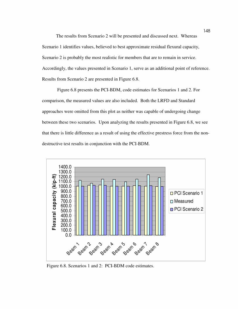
148

The results from Scenario 2 will be presented and discussed next. Whereas

Scenario 1 identifies values, believed to best approximate residual flexural capacity,

Scenario 2 is probably the most realistic for members that are to remain in service.

Accordingly, the values presented in Scenario 1, serve as an additional point of reference.

Results from Scenario 2 are presented in Figure 6.8.

Figure 6.8 presents the PCI-BDM, code estimates for Scenarios 1 and 2. For

comparison, the measured values are also included. Both the LRFD and Standard

approaches were omitted from this plot as neither was capable of undergoing change

between these two scenarios. Upon analyzing the results presented in Figure 6.8, we see

that there is little difference as a result of using the effective prestress force from the non-

destructive test results in conjunction with the PCI-BDM.

0.0100.0200.0300.0400.0500.0600.0700.0800.0900.0

1000.01100.01200.01300.01400.0

Beam

1

Beam

2

Beam

3

Beam

4

Beam

5

Beam

6

Beam

7

Beam

8

Fle

xu

ral

ca

pa

cit

y (

kip

-ft)

PCI Scenario 1

Measured

PCI Scenario 2

Figure 6.8. Scenarios 1 and 2: PCI-BDM code estimates.

149

Non-destructive values reported for the effective (residual) prestress force

were shown to be on average 94% of the values arrived at through the destructive tests

when the two outliers were eliminated.

Referring to Figure 6.9 we see that on average values for the PCI –BDM flexural

capacity remains unchanged. Both scenarios on average are 89% of the measured field

capacity. This is significant when one considers the fact that an in-service test can be

performed in lieu of a test that would render a member inadequate for in-service

conditions. This finding is tempered by the fact that Equation 32 is not overly sensitive

to nominal changes of fpe, the effective prestress force, after losses have been incurred,

as stated by Seguriant, Brice, and Khaleghi (2005).

Scenarios 1 and 2 present code estimates that are specific to each girder. Both

resulted in promising predictions; and in consequence, repeated iterations. Accordingly,

Scenario 3 explores the implication of using an average value for each of the various

parameters used in conjunction with a single iteration of the code(s). Figure 6.9 shows

the results for this condition.

Collectively, these results indicate that only negligible differences arise. Thus, the

engineer can use average values for section properties, effective prestress force, etc. As

was shown, average values used in conjunction with a single iteration of the code(s) is

just as effective at estimating the residual flexural capacity, as applying the code(s) to

individual members. Depending on the number of girders tested, and the number of codes

used, the former approach can save on time and money. Neither of these comes at the

expense of the code estimates.

150

Figure 6.9. Scenarios 1 through 3; code estimates for the flexural capacity.

Scenarios 1 through 3 reflect code behavior when parameters such as the

compressive strength of the deck and girder are known; as are the section properties, and

effective prestress forces. These scenarios require that a fair amount of field data must be

collected or is already available. The remaining scenarios reflect code behavior and

identify which parameters are most influential in providing accurate code estimates. The

following Table presents Scenarios 4 through 7 (Table 6.1).

151

Table 6.1. Parameters associated with scenarios 4 through 7

Scenario f'c Section Properties Pe

Scenario 4: Theoretical theoretical Pend Avg. measured

Scenario 5: Avg meas from cores theoretical theoretical

Scenario 6: Theoretical Avg. measured theoretical

Scenario 7: Theoretical theoretical theoretical

Qualitatively speaking, all theoretical parameters are those values that have been

specified on the plan sheets and are specific to this bridge. Quantitatively speaking, the

values associated with those parameters are listed in Table 6.2. Theoretical compressive

strengths of 3 and 5 ksi are noted for the deck and girder, respectively. Aside from a

prestressed centroid of 9 inches and an average deck height of 5 ½ inches, section

properties standard to an AASHTO Type II girder are used where theoretical properties

are called out. The effective prestress called out on the plan sheets was 169 kips, this is

taken as the theoretical value.

The average values, represent averages of field values collected for each

parameter. Here compressive strengths of 6.1 and 9.3 ksi are reported for the deck and

girder. Similarly, an average measured effective prestress force of 184.9 kips, based on

results from the non-destructive tests, and is used. Lastly, the average measured section

properties are presented in Table 6.2. The units associated with rows 2 through 10 are in

inches. The units associated with the last row, “Pend”, are in pounds. All things

considered, the section properties were fairly consistent amongst all eight girders.

Results specific to Scenarios 4 through 7 will be presented next in Figure 6.10.

1

52

Tab

le 6.2

Averag

es; measu

red sectio

n p

rop

erties associated

with

scenario

s 4 th

rough 7

.

9 5 8

7 1 8

9 3 4

7 5 4

7 1 8

9 6 0

7 7 4

9 3 6

8 0 1

7 7 4

1 0 1 4

8 9 4

9 8 9

9 1 7

8 9 0

0.0

200.0

400.0

600.0

800.0

1000.0

1200.0

L R F D ,S ce n 3

L R F D ,S ce n 4

L R F D ,S ce n 5

L R F D ,S ce n 6

L R F D ,S ce n 7

S T D ,S ce n 3

S T D ,S ce n 4

S T D ,S ce n 5

S T D ,S ce n 6

S T D ,S ce n 7

P C I,S ce n 3

P C I,S ce n 4

P C I,S ce n 5

P C I,S ce n 6

P C I,S ce n 7

fle x u ra l c a p a c ity (k ip -fe e t)

F

igu

re 6.1

0 F

lexural cap

acities, scenario

s 3 th

rough 7

.

153

For comparison, Scenario 3 was included in Figure 6.10 as all parameters were

known, from which the averages of each were used. Upon examining the data presented

in Figure 6.10 it is clear that each code predicted values closest to the measured capacity

when the field parameters were used throughout. Closer examination of Figure 6.10

reveals that of all the field parameter, the compressive strength of the deck and girder are

probably the most important when estimating the flexural capacity. The section properties

were shown to be the second most influential parameter. Scenario 7 represents when

theoretical, or rather, plan values were used throughout the code(s). There is a marked

difference (23 percent) between Scenarios 3 and 7. The take home message here is that

measured data plays an important role in estimating the flexural strength of prestressed

concrete bridge girders.

Although the effective prestress force was not as influential as the other

parameters presented in Table 6.1 for the PCI BDM, and did not play a factor in the other

two codes presented in Figure 6.10, its importance should not be underestimated. By

design, the code estimates are meant to be conservative. In light of this, being able to

directly determine the residual prestress force on in-service members means that actual

bridge capacities can be determined and do not have to be conservatively estimated.

Load deflection

As mentioned in the introduction, load and associated deflection readings are also

presented in this chapter. Herein, field data is presented alongside of predicted values for

deflection. This program incorporates moment-area concepts that are based on measured

material properties. The measured material properties include; the compressive strength

154

of the concrete; the type of prestressing steel; the type of mild reinforcement; and the

prestressing force. Armed with these material properties and field measurements, one

can create a model that accurately predicts the deflection of prestressed concrete

members placed under a load.

The computer program, RESPONSE, is used to generate moment curvature

diagrams. These moment curvature diagrams reflect the average cross-sectional

dimensions for all eight prestressed girders. Collectively, the average values were used

to create a single, representative cross section of an AASHTO Type II bridge girder that

was 388 sq. in. with 43 sq. in. of deck concrete placed atop. These dimensions reflect a

42 in. tall girder that is 18.5 in. at the base and 12.5 in. at the top. (Refer to Chapter 5 for

the strand locations and associated dimensions.) The cross section just described, was

used to generate moment curvature diagrams wherein only the prestressing force was

varied (Figure 6.11).

-600

-400

-200

0

200

400

600

800

1000

1200

-2500 -2000 -1500 -1000 -500 0 500 1000

Curvature (rad/10^6 in)

Mo

men

t C

ap

acit

y (

kip

-ft)

Figure 6.11. Moment curvature diagram for girders 1 and 2; three point loading.

155

The moment curvature diagram presented in Figure 6.11 reflects an average

prestressing force of 190.83 kips for girders 1 and 2. The average prestress force was

used to reflect the measured behavior for each pair of beams that was loaded through

failure under like loading conditions. As shown in Figure 6.11, a maximum moment of

1115 kip feet was recorded alongside a curvature of 285.7 rad/106 in. As a matter of

procedure, a number of moments and associated curvatures are read from a moment

curvature diagram, in this case Figure 6.11. The values read from such a diagram can be

used for virtually any type of applied load. Differences between the remaining moment

curvature diagrams were negligible and did not warrant individual plots. For a simply

supported beam, the applied load results in a corresponding moment over the length of a

beam. Figure 6.12, adopted from Collins and Mitchell (1997), presents such a scenario.

Figure 6.12. Moment and curvature for a simply supported beam.

156

As the moment is maximized at the mid-span, so to is the associated deflection.

This moment is a result of the applied load and associated distance. Both of these

concepts are emphasized in Figure 6.12. Because the moment and curvature diagrams

are mirrored for equidistant locations beyond mid-span, calculations are typically not

carried out beyond the mid-span of a beam. By integrating the moment diagram, the

curvature can be calculated for a given point. By integrating the curvature diagram, the

deflection can be calculated at a given point. Numerical integration can simplify the

process (Equation 6.17).

(6.17)

Deflection (∆) is solved for by taking nominal values for curvature (Фn),

multiplying each by its respective distance (xn), and repeating the procedure and adding it

to the values that correspond to the next point of interest. This product is divided by a

factor of 2 and multiplied by the resulting distance between each pair of points (∆xn).

Refer to Figure 6.12. The increments can be divided up until a necessary level of

accuracy is achieved. For this work a total of seven increments were used to solve for the

deflection at midspan, starting at the end.

The procedure just described is repeated for nominal loads until a desired number

of points can be plotted (Figure 6.13). Figure 6.13 presents the measured values for

girders 1 and 2, and compares these values to the predicted deflections using

RESPONSE. These girders reflect a three point loading scenario. The predicted values

are shown to closely approximate the measured values for both girders.

157

Figure 6.13. Load deflection diagram for girders 1 and 2.

As the load increased, predicted values resulted in slightly higher deflections

when compared to the measured values. At approximately 198,000 lbs, the predicted

deflection was 1.72 inches. This value can be compared to a load and associated

deflection of 215,000 lbs and 1.75 inches for Girder 1 and 210,000lbs and 1.63 inches for

Girder 2. The fact that Girders 1 and 2 plotted similar to one another indicates that the

prestressing force and associated losses were comparable. The load deflection diagram

for Girders 3 and 7 are presented next (Figure 6.14). Figure 6.14 presents the results for

the first 3, four point loading scenarios. This four point loading scheme reflects a constant

moment region of 2 feet oriented about the mid-span of these two girders. Here again, the

predicted values are shown to closely approximate the measured values for both girders.

As the load increased, predicted values resulted in slightly higher deflections when

158

compared to the measured values. At approximately 242,000 lbs, the predicted

deflection was 2.97 inches. This value can be compared to a load and associated

deflection of 242,000 lbs and 2.87 inches for Girder 3 and 236,700lbs and 2.71 inches for

Girder 2. The fact that Girders 3 and 7 plotted with increased separation indicates that

the prestressing force and associated losses differed by a slightly larger amount, 20,000

pound to be exact.

When compared to the results of Figure 6.13, the constant moment region results

in higher loads and higher deflections. The deflection at failure for both beams was still

comparable as shown in Figure 6.14. An average prestressing force of 210,000 lbs was

used for the predicted values associated with this model. The load deflection diagram for

Girders 4 and 5 are presented next (Figure 6.15).

Figure 6.14. Load deflection diagram for girders 3 and 7.

159

Figure 6.15. Load deflection diagram for girders 4 and 5.

Figure 6.15 presents the results for a four-point loading scheme with a constant

moment region of 6 feet oriented about the mid-span of these two girders. The predicted

values are shown to closely approximate the measured values for both girders up through

90,000 pounds. As the load increased, predicted values resulted in slightly higher

deflections when compared to the measured values. This deviation is attributed to a

larger constant moment region. Where measured values are analyzed, the larger constant

moment region corresponds to smaller deflections for a given load. Still, fairly accurate

predictions were provided near the ultimate moment capacity. At approximately

257,240 lbs, the predicted deflection was 2.27 inches. This value can be compared to a

load and associated deflection of 268,300 lbs and 2.02 inches for Girder 4 and 257,240lbs

and 1.51 inches for Girder 5.

160

When compared to the results of Figure 6.13, the constant moment region

results in higher loads and higher deflections. The deflection at failure for both beams

was still comparable as shown in Figure 6.14. An average prestressing force of 180,000

lbs was used for the predicted values associated with this model. The load deflection

diagram for Girders 6 and 8 are presented next (Figure 6.16).

Figure 6.16 presents the results for a four-point loading scheme with a constant

moment region of 9.5 feet oriented about the mid-span of these two girders. The

predicted values are shown to closely approximate the measured values for both girders

up through 130,000 pounds. As the load increased, predicted values resulted in slightly

higher deflections when compared to the measured values. This was also the finding for

Girders 4 and 5. At approximately 330,040 lbs, the predicted deflection was 2.86 in.

This value can be compared to a load and associated deflection of 340,020 lbs and 2.63

inches for Girder 6 and 330,040lbs and 2.14 in. for Girder 8. The difference in load and

associated deflection between Girders 6 and 8 reflect the fact that the displacement

transducer was located 30 in. away from the mid-span of the girder. An average

prestressing force of 200,750 lbs was used for the predicted values associated with this

model.

In summary, measured deflections for Girders 1 and 2 were 98% of the predicted

value at the measured flexural capacity. Girders 3 and 7 were 94% of the average,

predicted peak deflection. Similarly, Girders 4 and 5 were 81% of the predicted,

maximum deflection, on average. Lastly measured deflections for Girders 6 and 8 were

83% of the ultimate predicted deflection, on average. Collectively, the predicted values

overestimated the maximum deflections by 11% (Figure 6.17).

161

Figure 6.16. Load deflection diagram for girders 6 and 8. As indicated from the results presented in Figure 6.17, the peak deflections were shown

to overestimate measured deflections by an additional 14% when the constant moment

region increased beyond 2 feet. For a given load case, the measured deflections at

capacity were in close agreement with one another. For the three point loading applied at

midspan, Girders 1 and 2 were within 7% of one another. When a constant moment

region of 2 feet was introduced, Girders 3 and 7 were shown to be within 6% of one

another. When the constant moment region was increased to 6 feet, the measured

deflections for Girders 4 and 5 were shown to be within 23% of one another. This

difference is attributed to local variance in the compressive strength of concrete.

Maximum deflections for Girders 6 and 8 were shown to differ by nearly 19%.

162

0.00

0.50

1.00

1.50

2.00

2.50

3.00

3.50

Gird

er 1

Gird

er 2

Pre

dicte

d

Gird

er 3

Gird

er 7

Pre

dicte

d

Gird

er 4

Gird

er 5

Pre

dicte

d

Gird

er 6

Gird

er 8

Pre

dicte

d

Defl

ecti

on

(in

.)

Figure 6.17. Peak deflections for girders 1 through 8. When greater loads are incurred over longer spans, as is the case with increasing

constant moment regions, the localized variance of concrete’s compressive strength is

believed to be of greater significance.

Conclusions

During design, accurate prediction of the flexural capacity and associated

deflections under load are of great importance in the field of bridge engineering.

Implications of underestimating the flexural capacity during design can result in cracking

and service loads, and in worst case scenarios, failure of the prestressed member.

Overestimating the flexural capacity by a significant amount during design results in over

conservative designs, and unnecessary costs. The code estimates are meant to be

conservative. Alternatively, the residual prestress force for in-service members can be

determined directly through the non-destructive technique presented in this research. As

163

such, the service bridge capacities can also be determined directly and don’t have to

be conservatively estimated.

Results from the field tests indicated that all eight girders failed in a ductile

manner. The measured flexural capacities were all comparable to one another. The

average measured flexural capacity was 1149 kip-feet. The maximum and minimum

values were 1060 kip-feet for Girder 2, and 1243.9 kip-feet for Girder 7. The measured

flexural capacity was compared to code estimates such as the AASHTO LRFD, and

AASHTO Standard methods and the PCI-BDM method.

Results indicated that the PCI-BDM method provided the most accurate results

with an average overestimate of 11 percent. It was shown that in-service tests, performed

in lieu of destructive tests, do not result in reduced, analytical flexural capacities. The

same can be said for using an average value of the non-destructive tests and section

properties as only negligible differences arose (less than 1%). As such, average values

used in conjunction with a single iteration of the code(s) are just as effective at estimating

the residual flexural capacity. When theoretical, or rather, plan values were used

throughout the code(s), flexural capacities were 75% (LRFD), 81% (Standard), and 87%

(PCI-BDM) of the measured flexural capacity. Each code predicted values closest to the

measured capacity when average, measured values were used. The compressive

strengths of the deck and girder are probably the most influential when estimating the

flexural capacity. The section properties were shown to be the second most influential

parameter.

Load and associated deflection readings were also presented in this chapter. Here,

field data was presented alongside of predicted values. For predicted values, a computer

164

program was used to generate a moment curvature diagram. This program

incorporated moment-area concepts that are based on measured material properties.

Where peak deflections are considered, values were shown to overestimate the

measured deflections by 11 percent, on average. The measured deflections for a given

pair of girders behaved most similarly (within 10%) when failed under a three-point load,

or a small constant moment region of 2 feet. Overall, the computer program,

RESPONSE, accurately predicted deflections at in-service capacity as well as at

maximum capacity.

165

CHAPTER 7

CONCLUSIONS AND RECOMMENDATIONS

Conclusions

This research embodied a three-prong approach for directly determining the

residual prestress force of prestressed concrete bridge girders. For bridges that have yet

to be constructed, outfitting girders with instrumentation is a highly effective means of

determining residual prestress force in prestressed concrete bridge girders. This

constitutes the first prong. Four precast, prestressed girders made with high-performance,

self-consolidating concrete were instrumented and monitored for prestress losses. The

observed values of prestress losses were compared with values calculated using the

AASHTO LRFD Specifications (2004) and a newly proposed method based on the

results of the AASHTO LRFD-07 (Tadros et al., 2003). Overall the NCHRP method

proved to more closely approximate measured values when actual compressive strengths

were used.

Still, many bridges are constructed without such instrumentation. For these

bridges, a destructive technique can be used to directly determine the residual prestress in

a prestressed concrete bridge girder. This implies that the girder(s) being tested have

already been taken out of service. This constitutes the second prong. Two destructive

methods were employed to determine the residual prestress force; the more conservative

results were evidenced through the standard method; strain gauges placed to either side of

a crack. As previously indicated, instances may arise where a bilinear response isn’t

always exhibited in data collected from the standard approach. Here, the modified

166

approach (a strain gauge placed directly over a crack) could be used in lieu of the

standard approach.

Assuming both methods are used to determine the decompression load, it would

be safe to use the more conservative results. Depending on the response curves

generated, the method subject to the least amount of interpretation may also be preferred.

Now assuming both of these conditions are met through a single method, then the path is

clear. If not, engineering judgment is required.

For bridges that are anticipated to remain in service that are lacking embedded

instrumentation, the development of a non-destructive technique used to estimate the

remaining force in the tendons of prestressed bridge girders is extremely important. This

constitutes the third prong used to directly determine residual prestress force. Here a

strain gauge was oriented between two 1 ½ in. deep saw cuts. These cuts transverse the

entire width of the bottom flange and were placed ¼-in. to either side of the strain gauge.

This procedure was repeated twice at locations that were equal distances away from mid-

span. The average of both readings was then used to calculate the residual prestress force.

On average, the estimated residual prestress force as determined by the non-

destructive tests was 94% of the estimated residual prestress force as determined by the

destructive tests. Analytical estimates were closest to the destructive and non-destructive

test results using the Lump Sum Method. Both the AASHTO LRFD-04 and the

AASHTO LRFD-07 were shown to be un-conservative. Hence for girders with a service

life of 40 years, prestress losses were most accurately reflected in the procedure that

yielded the largest prestress loss.

167

The measured flexural capacity was also determined from field tests and

compared to analytical estimates such as the AASHTO LRFD code, the AASHTO

Standard code, and the Prestressed Concrete Institute Bridge Design Manual code (PCI-

BDM). A number of scenarios were considered. Each analytical method predicted values

closest to the measured capacity when average, measured values were used. Preference

was given to the PCI-BDM code as the predicted flexural capacity was 89% of the

average measured flexural capacity. The average measured flexural capacity was 1149

kip-feet. Where material properties can be accounted for, the compressive strengths of the

deck and girder have the most influence in accurately estimating the flexural capacity.

The section properties were shown to be the second most influential parameter.

By design, the code estimates are meant to be conservative. Alternatively, the

residual prestress force for in-service members can be determined directly through the

non-destructive technique presented in this research. As such, bridge capacity can also be

determined directly and doesn’t have to be conservatively estimated.

Where peak deflections are considered, values were shown to overestimate the

measured deflections by 11%, on average. Overall, the computer program, RESPONSE,

accurately predicted deflections at in-service capacity as well as at maximum capacity.

Recommendations

Currently, it is assumed that prestressing strands provide a uniform load

throughout the span of a girder once development lengths of 60-strand diameters have

been achieved from either end. Results from the non-destructive tests indicate that this

may not be the case. The destructive tests indicated that one strain gauge yielded higher

168

values of strain when compared to readings take from the other strain gauge.

Typically values from one gauge exceeded the target value associated with the

destructive test. The other strain gauge underestimated that same target value. When

averaged, the results behaved within 10% of the target values associated with the

destructive tests. Both strain gauges were located equal distances to either side of the

mid-span. Therefore, instrumenting a prestressed concrete bridge girder with multiple

strain gauges throughout the span may provide insight into why different readings were

likely, but why the average worked out.

The most practical method to implement the non-destructive method is to build a

guide track that extends beyond the width of the girder by a nominal amount and to

insure that a concrete saw capable of making 1 ½ in. deep cuts is used. Cuts should be

placed ¼ in. to either side of a 2-in. or 4-in. strain gauge and transverse the entire width

of the beam. It is recommended that these cuts be made in 1/8-in. increments and that

strain readings are collected in between each progressive set of cuts. A minimum of two

strain gauges should be placed on opposite sides, equidistant from midspan.

The next logical step for this research would be to perform the non-destructive

test on in-service members. As with the salvaged girders, care must be taken when

measuring section properties and determining compressive strengths of the deck and the

girder. The neutral axis may be field verified through a series of proof loads. Three

distinct loads are preferable and need not cause cracking in the bottom of a member. One

such advantage to this test arises in instances where coring the bridge girder is not a

feasible way to determine the compressive modulus of the girder. Here, deck cores and

results from the neutral axis test can be used to back out the modulus of the girder. This

169

assumes that the deck and girder are acting in a composite fashion and that a

transformation ratio is applied to obtain the neutral axis via hand calculations.

170

REFERENCES Ahlborn, T.M., C.K. Shield, and C.W. French. 1997, Full-scale testing of prestressed

concrete bridge girders. Experimental Techniques Journal 21(1):33-35. American Association of State Highway and Transportation Officials (AASHTO). 2004.

LRFD Bridge Design Specifications, Third Edition, Washington, D.C. Azizinamini, A., B. J. Keeler, J. Rohde, and A. B. Mehrabi. 1996. Application of a new

nondestructive evaluation technique to a 25-year-old prestressed concrete girder. Prestressed/Precast Concrete Institute Journal 41(3):82-95.

Barr, P. J., B. M. Kukay, and M. W. Halling. 2008. Comparison of prestress losses in a

high performance concrete bridge. Journal of Bridge Engineering, ASCE. In press.

Chen, R. H.L., and K. Wissawapaisal. 2001. Measurement of tensile forces in a seven-

wire prestressing strand using stress waves. Journal of Engineering Mechanics 127(6):599-606.

Civjan, Ss. A., J. O. Jirsa, R. L. Carrasquillo, and D. W. Fowler. 1998. Instrument to

evaluate remaining prestress in damaged prestressed concrete bridge girders. Prestressed/Precast Concrete Institute Journal 43(2):62-71.

Cole, H. A. 2000. Direct solution for elastic prestress loss in pretensioned concrete

girders. Practice Periodical on Structural Design and Construction 5(1):27-31. Collins, M. P., and D. Mitchell. 1997. Prestressed concrete structures. Response

Publications, Canada. 766 p. Ghorbanpoor, A. 1999. Evaluation of prestressed concrete girders using magnetic flux

leakage. Proceedings of the 1999 Structures Congress for Structural Engineering in the 21st Century, April 18- 21, 1999. p. 284-287.

Hasley, T. J., and R. Miller. 1996. Destructive testing of two forty-year old prestressed

concrete bridge beams. Precast/Prestressed Concrete Institute Journal 41(5):84-93.

Kwak, H., and Y. Seo. 2002. Numerical analysis of time-dependent behavior of pre-cast

prestressed concrete girder bridges. Construction and Building Materials Journal 16(1):49-63.

Labia, Y., M. S. Saiidi, and B. Douglas. 1997. Full-scale testing and analysis of 20-year-

old pretensioned concrete box girders. Structural Journal, ACI 94(5):471-482.

171

Lopez, M., L.F. Kahn, K. E. Kurtis, and J. S. Lai. 2003. Creep, shrinkage, and prestress

of high-performance precast prestressed bridge girders. Structural Engineering, Mechanics, and Materials Research Report No. 00-1, Georgia Institute of Technology, Atlanta GA.

Onyemelukwe, O., and M. Issa. 1997. Field measurement of time-dependent losses in

prestressed concrete bridges. Proceedings of the 1997 15th Structures Congress. April 13-16, 1997. p. 1569-1573.

Onyemelukwe, O.U., M. Issa, and C.J. Mills. 2003. Field measured prestress concrete

losses versus design code estimates. Journal of Experimental Mechanics 43(2):201-215.

Pandit, G.S., and S.P. Gupta. 1980. Free body approach for analysis of prestressed

concrete beams. Indian Concrete Journal 54(6):154-161. Pessiki, S., M. Kaczinski, and H. H. Wescott. 1996. Evaluation of effective prestress

force in 28-year-old prestressed concrete bridge beams. Prestressed/Precast Concrete Institue Journal 41(6):78-89.

Roller, J.J., H. G. Russell, R.N. Bruce, and B.T. Martin. 1995. Long-term performance

of prestressed, pretensioned high strength concrete bridge girders. Prestressed/Precast Concrete Institue Journal 40(6):48-59.

Scheel, H., and B. Hillemeir. 2003. Location of prestressing steel fractures in concrete.

Journal of Materials in Civil Engineering 15(5):228-234. Seguirant, S. J., R. Brice, and B. Khaleghi. 2005. Flexural strength of reinforced and

prestresed concrete t-beams. Precast/Prestressed Concrete Institute Journal 50(1):44-73.

Shams, M.K. and L.F. Kahn. 2000. Time-dependent behavior of high-strength concrete:

task 3, use of high strength/high performance concrete for precast prestressed concrete bridges in Georgia. Structural Engineering, Mechanics, and Materials Research Report No. 00-1, Georgia Institute of Technology, Atlanta GA.

Shenoy, C. V., and G. C. Frantz. 1991. Structural tests of 27-year-old prestressed

concrete bridge beams. Precast/Prestressed Concrete Institute Journal 36(5):80-90.

Tadros, M.K., N. Al-Omaishi, S.J. Seguirant, and J.G. Gallt. 2003. Prestress losses in

pretensioned high-strength concrete bridge girders. NCHRP Report 496, National Cooperative Highway Research Program, Transportation Research Board, National Research Council. August 2003, 111 p.

172

APPENDICES

173

Appendix A

Modulus of Elasticity

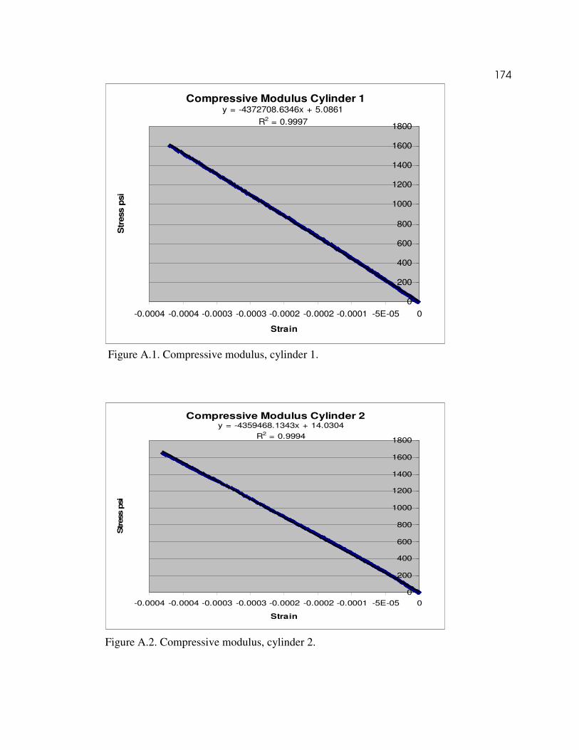
174

Figure A.1. Compressive modulus, cylinder 1.

Figure A.2. Compressive modulus, cylinder 2.

Compressive Modulus Cylinder 1y = -4372708.6346x + 5.0861

R2 = 0.9997

0

200

400

600

800

1000

1200

1400

1600

1800

-0.0004 -0.0004 -0.0003 -0.0003 -0.0002 -0.0002 -0.0001 -5E-05 0

Strain

Str

ess p

si

Compressive Modulus Cylinder 2y = -4359468.1343x + 14.0304

R2 = 0.9994

0

200

400

600

800

1000

1200

1400

1600

1800

-0.0004 -0.0004 -0.0003 -0.0003 -0.0002 -0.0002 -0.0001 -5E-05 0

Strain

Stress p

si

175

Figure A.3. Compressive modulus, cylinder 3. Figure A.4. Compressive modulus, cylinder 4.

Compressive Modulus Cylinder 3y = -4754340.6837x + 8.0855

R2 = 0.9992

0

200

400

600

800

1000

1200

1400

1600

1800

-0.0004 -0.0004 -0.0003 -0.0003 -0.0002 -0.0002 -0.0001 -5E-05 0

Strain

Str

ess p

si

Compressive Modulus Cylinder 4y = -4042294.0319x + 10.8350

R2 = 0.9992

0

200

400

600

800

1000

1200

1400

1600

1800

-0.0005 -0.0004 -0.0003 -0.0002 -0.0001 0

Strain

Str

ess p

si

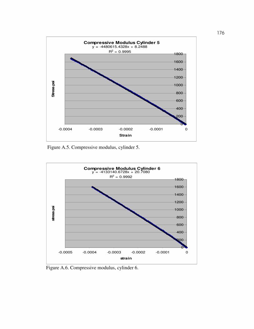
176

Figure A.5. Compressive modulus, cylinder 5. Figure A.6. Compressive modulus, cylinder 6.

Compressive Modulus Cylinder 5y = -4480615.4328x + 8.2488

R2 = 0.9995

0

200

400

600

800

1000

1200

1400

1600

1800

-0.0004 -0.0003 -0.0002 -0.0001 0

Strain

Str

ess p

si

Compressive Modulus Cylinder 6y = -4133140.6728x + 20.7080

R2 = 0.9992

0

200

400

600

800

1000

1200

1400

1600

1800

-0.0005 -0.0004 -0.0003 -0.0002 -0.0001 0

strain

stress p

si

177

Figure A.7. Compressive modulus, cylinder 7. Figure A.8. Compressive modulus, cylinder 8.

Compressive Modulus Cylinder 7y = -4311455.1027x + 15.9549

R2 = 0.9994

0

200

400

600

800

1000

1200

1400

1600

1800

-0.0005 -0.0004 -0.0003 -0.0002 -0.0001 0

Strain

Str

ess p

si

Compressive Modulus Cylinder 8y = -4132530.9697x + 5.6314

R2 = 0.9996

0

200

400

600

800

1000

1200

1400

1600

1800

-0.0005 -0.0004 -0.0003 -0.0002 -0.0001 0

Strain

Str

ess p

si

178

Figure A.9. Compressive modulus, cylinder 9.

Figure A.10. Compressive modulus, cylinder 4 (chapter 4).

Cylinder 4 Diam (in) Rad (in) Area (sq in)

4.048 2.024 12.86977

S2 2530.65147 psi

S1 106.2291 psi

e1 0.000005263 strain

e2 0.000540789 strain

E = (S2-S1)/(e2-e1)

Corrected E 4527176.91 psi

E 4527.17691 ksi

Compressive Modulus Cylinder 9y = -4310822.4471x + 12.4366

R2 = 0.9989

0

200

400

600

800

1000

1200

1400

1600

1800

-0.0004 -0.0003 -0.0002 -0.0001 0

Strain

Stress p

si

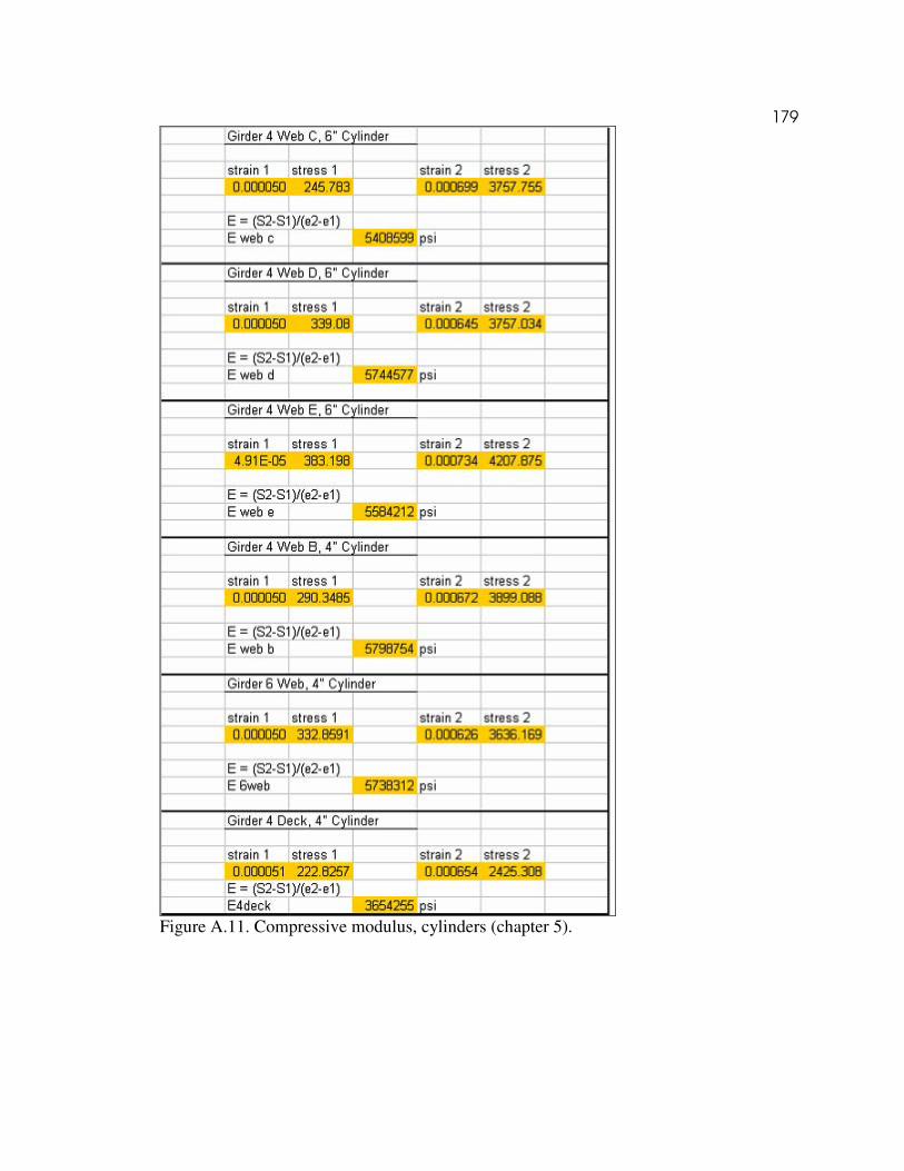
179

Figure A.11. Compressive modulus, cylinders (chapter 5).

180

Appendix B

Response to Neutral Axes

181

Beam 2 Neutral Axis

0

5

10

15

20

25

30

35

-150 -100 -50 0 50 100 150

micro strain

dis

t fr

om

bo

tom

(in

)

25 K

50 K

75 K

Neutral axis 17.5 inches from

bottom (calculated w as 18.5

inches).

Figure B.1. Neutral axis, beam 2.

Beam 3 Neutral Axis

0

5

10

15

20

25

30

35

-200 -150 -100 -50 0 50 100 150 200

micro strain

dis

t fr

om

bo

tom

(in

)

25 K

50 K

75 K

Neutral axis 17.25 inches from

bottom (calculated w as 18.38

inches).

Figure B.2. Neutral axis, beam 3.

182

Beam 4 Neutral Axis

0

5

10

15

20

25

30

35

-300 -250 -200 -150 -100 -50 0 50 100 150

micro strain

dis

t fr

om

bo

tom

(in

)

25 K

50 K

75 K

Neutral axis 17 inches from

bottom (calculated w as

18.19 inches).

Figure B.3. Neutral axis, beam 4.

Beam 5 Neutral Axis

0

5

10

15

20

25

30

35

-100 -50 0 50 100 150 200

micro strain

dis

t fr

om

bo

tom

(in

)

25 K

50 K

75 K

Neutral axis 17 inches from bottom (calculated

w as 18.17 inches).

Figure B.4. Neutral axis, beam 5.

183

Beam 6 Neutral Axis

0

5

10

15

20

25

30

35

-150 -100 -50 0 50 100 150

micro strain

dis

t fr

om

bo

tom

(in

)

25 K

50 K

75 K

Neutral axis 17.5 inches from

bottom (calculated w as 18.31

inches).

Figure B.5. Neutral axis, beam 6.

Beam 7 Neutral Axis

0

5

10

15

20

25

30

35

-150 -100 -50 0 50 100 150

micro strain

dis

t fr

om

bo

tom

(in

)

25 K

50 K

75 K

Neutral axis 18.5 inches from

bottom (calculated w as 18.2

inches).

Figure B.6. Neutral axis, beam 7.

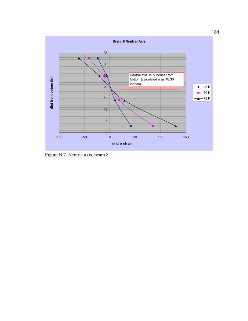
184

Beam 8 Neutral Axis

0

5

10

15

20

25

30

35

-100 -50 0 50 100 150

micro strain

dis

t fr

om

bo

tom

(in

)

25 K

50 K

75 K

Neutral axis 19.5 inches from

bottom (calculated w as 18.30

inches).

Figure B.7. Neutral axis, beam 8.

185

Appendix C

Response to Decompression Loads

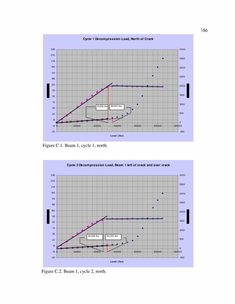
186

Cycle 1 Decompression Load, North of Crack

-30

-10

10

30

50

70

90

110

130

150

170

190

210

230

250

0 20000 40000 60000 80000 100000 120000

Load ( lbs)

-500

0

500

1000

1500

2000

2500

3000

3500

4000

51,250 lbs 55,000 lbs

Figure C.1. Beam 1, cycle 1, north.

Cycle 2 Decompression Load, Beam 1 left of crack and over crack

-30

-10

10

30

50

70

90

110

130

150

170

190

210

230

250

0 20000 40000 60000 80000 100000 120000

Load ( lbs)

-500

0

500

1000

1500

2000

2500

3000

3500

4000

46,250 lbs 50,000 lbs

Figure C.2. Beam 1, cycle 2, north.

187

Cycle 2 Decompression Load, Beam 1, Right of Crack

-30

-10

10

30

50

70

90

110

130

150

170

190

210

230

250

0 20000 40000 60000 80000 100000 120000

Load ( lbs)

-500

0

500

1000

1500

2000

2500

3000

3500

4000

50,000 lbs 52,500 lbs

Figure C.3. Beam 1, cycle 2, south.

Cycle 3 Decompression Load, Beam 1 ,Left of Crack

-30

-10

10

30

50

70

90

110

130

150

170

190

210

230

250

0 20000 40000 60000 80000 100000 120000

Load ( lbs)

-500

0

500

1000

1500

2000

2500

3000

3500

4000

46,250 lbs 50,000 lbs

Figure C.4. Beam 1, cycle 3, north.

188

Cycle 3 Decompression Load, Beam 1 Right of crack and over crack

-30

-10

10

30

50

70

90

110

130

150

170

190

210

230

250

0 20000 40000 60000 80000 100000 120000

Load (lbs)

mic

rostr

ain

-500

0

500

1000

1500

2000

2500

3000

3500

4000

mic

rostr

ain

50,000 lbs 52,500 lbs

Figure C.5. Beam 1, cycle 3, south.

Cycle 4 Decompression Load, Beam 1, Left of Crack

-30

-10

10

30

50

70

90

110

130

150

170

190

210

230

250

0 20000 40000 60000 80000 100000 120000

Load (lbs)

mic

rostr

ain

-500

0

500

1000

1500

2000

2500

3000

3500

4000

mic

rostr

ain

46,250 lbs 50,000 lbs

Figure C.6. Beam 1, cycle 4, north.

189

Cycle 4 Decompression Load, Beam 1 Right of crack and over crack

-30

-10

10

30

50

70

90

110

130

150

170

190

210

230

250

0 20000 40000 60000 80000 100000 120000

Load (lbs)

mic

rostr

ain

-500

0

500

1000

1500

2000

2500

3000

3500

4000

mic

rostr

ain

50,000

lbs52,500

lbs

Figure C.7. Beam 1, cycle 4, south.

Beam 2, Cycle 1 Decompression Load, left of crack

-30

-10

10

30

50

70

90

110

130

150

170

190

210

230

250

0 20000 40000 60000 80000 100000 120000

Load (lbs)

mic

rostr

ain

-500

0

500

1000

1500

2000

2500

3000

3500

4000

mic

rostr

ain

50,000 lbs

Figure C.8. Beam 2, cycle 1, north.

190

Beam 2, Cycle 1 Decompression Load, right of crack

-10

10

30

50

70

90

110

130

150

170

190

210

230

250

0 20000 40000 60000 80000 100000 120000

Load (lbs)

mic

rostr

ain

-500

0

500

1000

1500

2000

2500

3000

3500

4000

mic

rostr

ain

50,000 lbs

58,750 lbs

Figure C.9. Beam 2, cycle 1, south.

Beam 2, Cycle 2 Decompression Load, Left of Crack

-30

-10

10

30

50

70

90

110

130

150

170

190

210

230

250

0 20000 40000 60000 80000 100000 120000

Load (lbs)

mic

rostr

ain

-500

0

500

1000

1500

2000

2500

3000

3500

4000

mic

rostr

ain

50,000 lbs 55,000 lbs

Figure C.10. Beam 2, cycle 2, north.

191

Beam 2, Cycle 2 Decompression Load, right of crack

-30

-10

10

30

50

70

90

110

130

150

170

190

210

230

250

0 20000 40000 60000 80000 100000 120000

Load (lbs)

mic

rostr

ain

-500

0

500

1000

1500

2000

2500

3000

3500

4000

mic

rostr

ain

55,000 lbs

Figure C.11. Beam 2, cycle 2, south.

Beam 2, Cycle 3 Decompression Load, Left of Crack

-10

10

30

50

70

90

110

130

150

170

190

210

230

250

0 20000 40000 60000 80000 100000 120000

Load (lbs)

mic

rostr

ain

-500

0

500

1000

1500

2000

2500

3000

3500

4000

mic

rostr

ain

55,000

lbs

Figure C.12. Beam 2, cycle 3, north.

192

Beam 2, Cycle 3 Decompression Load, right of crack

-30

-10

10

30

50

70

90

110

130

150

170

190

210

230

250

0 20000 40000 60000 80000 100000 120000

Load (lbs)

mic

rostr

ain

-500

0

500

1000

1500

2000

2500

3000

3500

4000

mic

rostr

ain

55,000 lbs

Figure C.13. Beam 2, cycle 3, south.

Beam 3, Cycle 3 Decompression Load, left of crack

-30

-10

10

30

50

70

90

110

130

150

170

190

210

230

250

0 20000 40000 60000 80000 100000 120000

Load (lbs)

mic

rostr

ain

-500

0

500

1000

1500

2000

2500

3000

3500

4000

mic

rostr

ain

70,000

lbs

60,000

lbs

Figure C.14. Beam 3, cycle 3, north.

193

Beam 3, Cycle 3 Decompression Load, right of crack

-30

-10

10

30

50

70

90

110

130

150

170

190

210

230

250

0 20000 40000 60000 80000 100000 120000

Load (lbs)

mic

rostr

ain

-500

0

500

1000

1500

2000

2500

3000

3500

4000

mic

rostr

ain

50,000

lbs

60,000

lbs

Figure C.15. Beam 3, cycle 3, south.

Beam 3, Cycle 4 Decompression Load, Left of crack

-30

-10

10

30

50

70

90

110

130

150

170

190

210

230

250

0 20000 40000 60000 80000 100000 120000

Load (lbs)

mic

rostr

ain

-500

0

500

1000

1500

2000

2500

3000

3500

4000

mic

rostr

ain

70,000 lbs60,000 lbs

Figure C.16. Beam 3, cycle 4, north.

194

Beam 3, Cycle 4 Decompression Load, right of crack

-30

-10

10

30

50

70

90

110

130

150

170

190

210

230

250

0 20000 40000 60000 80000 100000 120000

Load (lbs)

mic

rostr

ain

-500

0

500

1000

1500

2000

2500

3000

3500

4000

mic

rostr

ain

45,000 lbs60,000 lbs

Figure C.17. Beam 3, cycle 4, south.

Beam 3, Cycle 5 Decompression Load, left of crack

-30

-10

10

30

50

70

90

110

130

150

170

190

210

230

250

0 20000 40000 60000 80000 100000 120000

Load (lbs)

mic

rostr

ain

-500

0

500

1000

1500

2000

2500

3000

3500

4000

mic

rostr

ain

72,500

lbs60,000

lbs

Figure C.18. Beam 3, cycle 5, north.

195

Beam 3, Cycle 5 Decompression Load, right of crack

-30

-10

10

30

50

70

90

110

130

150

170

190

210

230

250

0 20000 40000 60000 80000 100000 120000

Load (lbs)

mic

rostr

ain

-500

0

500

1000

1500

2000

2500

3000

3500

4000

mic

rostr

ain

50,000 lbs

60,000 lbs

Figure C.19. Beam 3, cycle 5, south.

Beam 4, Cycle 1 Decompression Load, Left of Crack

-30

-10

10

30

50

70

90

110

130

150

170

190

210

230

250

0 20000 40000 60000 80000 100000 120000

Load (lbs)

mic

rostr

ain

-500

0

500

1000

1500

2000

2500

3000

3500

4000

mic

rostr

ain

52,500 lbs50,000 lbs

Figure C.20. Beam 4, cycle 1, north.

196

Beam 4, Cycle 1 Decompression Load, Right of crack

-30

-10

10

30

50

70

90

110

130

150

170

190

210

230

250

0 20000 40000 60000 80000 100000 120000

Load (lbs)

mic

rostr

ain

-500

0

500

1000

1500

2000

2500

3000

3500

4000

mic

rostr

ain

53,750

lbs

50,000

lbs

Figure C.21. Beam 4, cycle 1, south.

Beam 4, Cycle 2 Decompression Load, Left of Crack

-30

-10

10

30

50

70

90

110

130

150

170

190

210

230

250

0 20000 40000 60000 80000 100000 120000

Load (lbs)

mic

rostr

ain

-500

0

500

1000

1500

2000

2500

3000

3500

4000

mic

rostr

ain

55,000

lbs

45,000

lbs

Figure C.22. Beam 4, cycle 2, north.

197

Beam 4, Cycle 2 Decompression Load, Right of crack

-30

-10

10

30

50

70

90

110

130

150

170

190

210

230

250

0 20000 40000 60000 80000 100000 120000

Load (lbs)

mic

rostr

ain

-500

0

500

1000

1500

2000

2500

3000

3500

4000

mic

rostr

ain

55,000

lbs

45,000

lbs

Figure C.23. Beam 4, cycle 2, south.

Beam 4, Cycle 3 Decompression Load, Left of Crack

-30

-10

10

30

50

70

90

110

130

150

170

190

210

230

250

0 20000 40000 60000 80000 100000 120000

Load (lbs)

mic

rostr

ain

-500

0

500

1000

1500

2000

2500

3000

3500

4000

mic

rostr

ain

55,000

lbs50,000

lbs

Figure C.24. Beam 4, cycle 3, north.

198

Beam 4, Cycle 3 Decompression Load, Right of crack

-30

-10

10

30

50

70

90

110

130

150

170

190

210

230

250

0 20000 40000 60000 80000 100000 120000

Load (lbs)

mic

rostr

ain

-500

0

500

1000

1500

2000

2500

3000

3500

4000

mic

rostr

ain

55,000

lbs

Figure C.25. Beam 4, cycle 3, south.

Beam 5, Cycle 1 Decompression Load, Left of Crack

-30

-10

10

30

50

70

90

110

130

150

170

190

210

230

250

0 20000 40000 60000 80000 100000 120000

Load (lbs)

mic

rostr

ain

-500

0

500

1000

1500

2000

2500

3000

3500

4000

mic

rostr

ain

50,000 lbs 52,500 lbs

Figure C.26. Beam 5, cycle 1, north.

199

Beam 5, Cycle 1 Decompression Load, Right of crack

-30

-10

10

30

50

70

90

110

130

150

170

190

210

230

250

0 20000 40000 60000 80000 100000 120000

Load (lbs)

mic

rostr

ain

-500

0

500

1000

1500

2000

2500

3000

3500

4000

mic

rostr

ain

50,000

lbs

Figure C.27. Beam 5, cycle 1, south.

Beam 5, Cycle 2 Decompression Load, Left of Crack

-30

-10

10

30

50

70

90

110

130

150

170

190

210

230

250

0 20000 40000 60000 80000 100000 120000

Load (lbs)

mic

rostr

ain

-500

0

500

1000

1500

2000

2500

3000

3500

4000

mic

rostr

ain

50,000

lbs

Figure C.28. Beam 5, cycle 2, north.

200

Beam 5, Cycle 2 Decompression Load, Right of crack

-30

-10

10

30

50

70

90

110

130

150

170

190

210

230

250

0 20000 40000 60000 80000 100000 120000

Load (lbs)

mic

rostr

ain

-500

0

500

1000

1500

2000

2500

3000

3500

4000

mic

rostr

ain

50,000

lbs

43,750

lbs

Figure C.29. Beam 5, cycle 2, south.

Beam 5, Cycle 3 Decompression Load, Left of Crack

-30

-10

10

30

50

70

90

110

130

150

170

190

210

230

250

0 20000 40000 60000 80000 100000 120000

Load (lbs)

mic

rostr

ain

-500

0

500

1000

1500

2000

2500

3000

3500

4000

mic

rostr

ain

51,250

lbs50,000

lbs

Figure C.30. Beam 5, cycle 3, north.

201

Beam 5, Cycle 3 Decompression Load, Right of crack

-30

-10

10

30

50

70

90

110

130

150

170

190

210

230

250

0 20000 40000 60000 80000 100000 120000

Load (lbs)

mic

rostr

ain

-500

0

500

1000

1500

2000

2500

3000

3500

4000

mic

rostr

ain

45,000

lbs

50,000

lbs

Figure C.31. Beam 5, cycle 3, south.

Beam 6, Cycle 1 Decompression Load, Right of crack

-30

-10

10

30

50

70

90

110

130

150

170

190

210

230

250

0 20000 40000 60000 80000 100000 120000

Load (lbs)

mic

rostr

ain

-500

0

500

1000

1500

2000

2500

3000

3500

4000

mic

rostr

ain

55,000

lbs

Figure C.32. Beam 6, cycle 1, north.

202

Beam 6, Cycle 1 Decompression Load, Right of crack

-30

-10

10

30

50

70

90

110

130

150

170

190

210

230

250

0 20000 40000 60000 80000 100000 120000

Load (lbs)

mic

rostr

ain

-500

0

500

1000

1500

2000

2500

3000

3500

4000

mic

rostr

ain

55,000

lbs

Figure C.33. Beam 6, cycle 1, south.

Beam 6, Cycle 2 Decompression Load, Left of Crack

-30

-10

10

30

50

70

90

110

130

150

170

190

210

230

250

0 20000 40000 60000 80000 100000 120000

Load (lbs)

mic

rostr

ain

-500

0

500

1000

1500

2000

2500

3000

3500

4000

mic

rostr

ain

53,750

lbs

55,000

lbs

Figure C.34. Beam 6, cycle 2, north.

203

Beam 6, Cycle 2 Decompression Load, Right of crack

-30

-10

10

30

50

70

90

110

130

150

170

190

210

230

250

0 20000 40000 60000 80000 100000 120000

Load (lbs)

mic

rostr

ain

-500

0

500

1000

1500

2000

2500

3000

3500

4000

mic

rostr

ain

55,000

lbs52,500

lbs

Figure C.35. Beam 6, cycle 2, south.

Beam 6, Cycle 3 Decompression Load, Left of Crack

-30

-10

10

30

50

70

90

110

130

150

170

190

210

230

250

0 20000 40000 60000 80000 100000 120000

Load (lbs)

mic

rostr

ain

-500

0

500

1000

1500

2000

2500

3000

3500

4000

mic

rostr

ain

55,000

lbs53,750

lbs

Figure C.36. Beam 6, cycle 3, north.

204

Beam 6, Cycle 3 Decompression Load, Right of crack

-30

-10

10

30

50

70

90

110

130

150

170

190

210

230

250

0 20000 40000 60000 80000 100000 120000

Load (lbs)

mic

rostr

ain

-500

0

500

1000

1500

2000

2500

3000

3500

4000

mic

rostr

ain

52,500

lbs

55,000

lbs

Figure C.37. Beam 6, cycle 3, south.

Beam 7, Cycle 1 Decompression Load, Left of Crack

-30

-10

10

30

50

70

90

110

130

150

170

190

210

230

250

0 20000 40000 60000 80000 100000 120000

Load (lbs)

mic

rostr

ain

-500

0

500

1000

1500

2000

2500

3000

3500

4000

mic

rostr

ain

60,000

lbs

58,750

lbs

Figure C.38. Beam 7, cycle 1, north.

205

Beam 7, Cycle 1 Decompression Load, Right of crack

-30

-10

10

30

50

70

90

110

130

150

170

190

210

230

250

0 20000 40000 60000 80000 100000 120000

Load (lbs)

mic

rostr

ain

-500

0

500

1000

1500

2000

2500

3000

3500

4000

mic

rostr

ain

58,750

lbs

60,000

lbs

Figure C.39. Beam 7, cycle 1, south.

Beam 7, Cycle 2 Decompression Load, Left of Crack

-30

-10

10

30

50

70

90

110

130

150

170

190

210

230

250

-20000 0 20000 40000 60000 80000 100000 120000

Load (lbs)

mic

rostr

ain

-500

0

500

1000

1500

2000

2500

3000

3500

4000

mic

rostr

ain

60,000

lbs

61,250

lbs

Figure C.40. Beam 7, cycle 2, north.

206

Beam 7, Cycle 2 Decompression Load, Right of crack

-30

-10

10

30

50

70

90

110

130

150

170

190

210

230

250

0 20000 40000 60000 80000 100000 120000

Load (lbs)

mic

rostr

ain

-500

0

500

1000

1500

2000

2500

3000

3500

4000

mic

rostr

ain

61,250

lbs60,000

lbs

Figure C.41. Beam 7, cycle 2, south.

Beam 7, Cycle 3 Decompression Load, Left of Crack

-30

-10

10

30

50

70

90

110

130

150

170

190

210

230

250

0 20000 40000 60000 80000 100000 120000

Load (lbs)

mic

rostr

ain

-500

0

500

1000

1500

2000

2500

3000

3500

4000

mic

rostr

ain

65,000

lbs60,000

lbs

Figure C.42. Beam 7, cycle 3, north.

207

Beam 7, Cycle 3 Decompression Load, Right of crack

-30

-10

10

30

50

70

90

110

130

150

170

190

210

230

250

0 20000 40000 60000 80000 100000 120000

Load (lbs)

mic

rostr

ain

-500

0

500

1000

1500

2000

2500

3000

3500

4000

mic

rostr

ain

61,250

lbs

65,000

lbs

Figure C.43. Beam 7, cycle 3, south.

Beam 8, Cycle 1 Decompression Load, Left of Crack

-30

-10

10

30

50

70

90

110

130

150

170

190

210

230

250

0 20000 40000 60000 80000 100000 120000

Load (lbs)

mic

rostr

ain

-500

0

500

1000

1500

2000

2500

3000

3500

4000

mic

rostr

ain

70,000

lbs50,000

lbs

Figure C.44. Beam 8, cycle 1, north.

208

Beam 8, Cycle 1 Decompression Load, Right of crack

-30

-10

10

30

50

70

90

110

130

150

170

190

210

230

250

0 20000 40000 60000 80000 100000 120000

Load (lbs)

mic

rostr

ain

-500

0

500

1000

1500

2000

2500

3000

3500

4000

mic

rostr

ain

70,000

lbs

Figure C.45. Beam 8, cycle 1, south.

Beam 8, Cycle 2 Decompression Load, Left of Crack

-30

-10

10

30

50

70

90

110

130

150

170

190

210

230

250

0 20000 40000 60000 80000 100000 120000

Load (lbs)

mic

rostr

ain

-500

0

500

1000

1500

2000

2500

3000

3500

4000

mic

rostr

ain

57,500 65,000

Figure C.46. Beam 8, cycle 2, north.

209

Beam 8, Cycle 2 Decompression Load, Right of crack

-30

-10

10

30

50

70

90

110

130

150

170

190

210

230

250

0 20000 40000 60000 80000 100000 120000

Load (lbs)

mic

rostr

ain

-500

0

500

1000

1500

2000

2500

3000

3500

4000

mic

rostr

ain

65,000

lbs55,000

lbs

Figure C.47. Beam 8, cycle 2, south.

Beam 8, Cycle 3 Decompression Load, Left of Crack

-30

-10

10

30

50

70

90

110

130

150

170

190

210

230

250

0 20000 40000 60000 80000 100000 120000

Load (lbs)

mic

rostr

ain

-500

0

500

1000

1500

2000

2500

3000

3500

4000

mic

rostr

ain

65,000

lbs

Figure C.48. Beam 8, cycle 3, north.

210

Beam 8, Cycle 3 Decompression Load, Right of crack

-30

-10

10

30

50

70

90

110

130

150

170

190

210

230

250

0 20000 40000 60000 80000 100000 120000

Load (lbs)

mic

rostr

ain

-500

0

500

1000

1500

2000

2500

3000

3500

4000

mic

rostr

ain

55,000

lbs

65,000

lbs

Figure C.49. Beam 8, cycle 3, south.

211

VITA

~ Brian M. Kukay ~ Department of Civil and Environmental Engineering

4110 Old Main Hill Logan UT 84322-4110

(435)797-2932

~ Education ~

MONTANA TECH OF THE UNIVERSITY OF MONTANA, Butte Montana B.S. ~ Environmental Engineering, 1999 M.S. ~ General Engineering, 2005

UTAH STATE UNIVERSITY, Logan Utah

Ph.D. ~ Civil and Environmental Engineering, 2008

Area of Specialization: Structural Engineering

~ Awards and Honors ~

Tau Beta Pi, National Engineering Honor Society, 2004 American Concrete Institute, Intermountain Chapter Graduate Scholarship Recipient, 2006 United States Department of Transportation, University Transportation Centers Program,“Outstanding Student of the Year” for the Utah Transportation Center, 2006 Golden Key International Honour Society, 2007 Cambridge Who’s Who Among Executives and Professionals, Honors Edition, 2007 - 2008

~ Teaching Experience ~

Teaching Assistant: Montana Tech of the University of Montana, 2003 – 2004 Laboratory assistance and grading for the strengths and mechanics of materials laboratory.

Instructor: Montana Tech of the University of Montana, 2004 – 2005

Sole responsibility for laboratory in strengths and mechanics of materials. Incorporated lectures and assisted in developing new curriculum.

212

Proctor: Montana Tech of the University of Montana, 2004 – 2005 Fundamentals of Engineering exam for the October, 2004 and April, 2005 sessions.

Lecturer: Utah State University, 2006 – 2007

Guest lectured for courses in experimental methods (graduate level) and reinforced concrete design (undergraduate level). Proctored exams for statics. Also hosted an outdoor field session for bridge design (graduate level).

Host: Engineering State, Utah State University 2006 – 2007

Facilitated several sessions of this outreach program for the Structures Division at Utah State University. Introduced high-school students throughout Utah to various projects, videos, and software packages that related to structural engineering.

Co-Instructor: Utah State University, 2008

Scheduled to co-teach a surveying course during the 2008 summer session. Includes lectures and field outings; with Dr. Joseph A. Caliendo.

~ Teaching Interests ~

General Engineering Courses: Statics, strengths and mechanics of materials, fluid mechanics, structural analysis and design, and mechanics of composite materials.

Code Based Design Courses:

Reinforced concrete design, steel design, and wood design.

~ Professional Affiliations ~

Engineer-In-Training: 2002. Seismic Effects, Friend of the Committee: 2007. Methods of Monitoring and Evaluating Structural Performance, Friend of the Committee: 2007. American Society of Civil Engineers, Student Member: 2007. Forest Products Society, Student Member: 2007.

213

~ Professional Experience ~

Bentley Construction Company, Inc., Butte, Montana October, 1998 – June 2000

Engineer Assist in preparing costs for bids on commercial projects, review contracts, read blueprints, create marketing materials.

Project Manager

Managed a $223,000 municipal wastewater treatment facility project.

Responsible for project layout, monitoring and compliance issues, confined space

issues, subcontractor and general supervision, contract negotiation, and hands-on

training.

Safety Director

Conducted weekly safety meetings. Responsible for creating and implementing

safety programs including: an incentive program, a voluntary respirator program,

an excavation program, and a hazards communication program.

BIO-WEST, Inc., Logan, Utah June 2000 – April 2003 full time –August 2003 part time

Project Engineer: Adept at compiling and submitting various permits and design calculations. Conducted: site assessments; project inspections; soil/gas surveys; phase I/II investigations and a corrective action analysis. Responsible for excavations, tank pulls, and monitoring well installations. Coordinated field aspects of various remediation system installations and modifications. Carried out several sampling events and reporting activities. Provided training for new employees on sampling protocol and “operation and maintenance” procedures. Also hosted numerous site walkthroughs and company meetings.

Project Manager:

Provide technical over-site, coordination of sub-contractors, and clientele expansion. During my most recent year of full time employment, I managed four projects, settled two payment disputes, and served as an assistant project manager on two leaking underground storage tank (LUST) sites in Utah. From 2002 to 2003, BIO-WEST was awarded contracts on eleven of the fifteen proposals that I compiled costs for.

214

~ Outside Interests ~

Tae-Kwon-Do: 20 years of experience, earned a third degree black belt while a student at Montana Tech. Also developed and instructed a self-defense course offered through Montana Tech’s Continuing Education Program, from 1994 to 2000. Camping and Cross Country Skiing: I enjoy camping with family and friends in the Pioneer Mountains and skiing in the Mount Hagen and Lost Trail wilderness areas. Sporting Events: I like attending local basketball and football games. Do-It-Yourself Projects and Wood-Working: I enjoy designing and constructing decks, board walks, and planters around the home. For my next project I plan on building a strip canoe.

~ Research Experience ~

Graduate Research, Montana Tech of the University of Montana and Utah State University: 2004 – 2007 (Research advisors: Dr. Leroy Friel, Dr. Paul Barr, and Dr. Dan Coster)

Quantify fires effect on wood products and composite wood products used in residential construction through measures of central tendency and dispersion: Montana Tech of the University of Montana, 2004 – 2005. Develop baseline prediction equations that can be compared with field data during post-fire evaluations through multivariate analyses. Equations such as this provide valuable analytical tools for inspection professionals; as they represent the mean residual flexural properties for specific materials and adjust for differences in specific gravity, an underlying factor of wood strength. Utah State University, 2005 - 2007.

Doctoral Research, Utah State University: 2005 - 2008 (research advisor: Dr. Paul Barr)

Perform a research program to determine the residual stress in full scale concrete bridge girders. Investigate the appropriateness of newly developed destructive and non-destructive techniques for the Utah Department of Transportation, 2005 - present. Monitor the behavior of a two-span, prestressed concrete bridge by embedding instrumentation in several bridge girders. Measured changes in strain are used to determine prestress loss values for each of the instrumented girders and are then compared to predictive values, 2005 - 2007.

215

~ Research Interests ~

Development and application of experimental destructive and non-destructive techniques used to evaluate wood structures. Development and application of experimental destructive and non-destructive techniques used to evaluate concrete structures.

~ Publications and Presentations ~

Barr, Paul J., Brian M. Kukay, and Marv W. Halling. Comparison of prestress losses for a prestress concrete bridge made with high performance concrete. American Society of Civil Engineer’s Journal of Bridges. Submitted for publication in July, 2006, under review. Barr, Paul J., Brian M. Kukay, and Marv W. Halling. 2007. A comparison of time dependent prestress losses in a two-span, prestressed concrete bridge. Presented at the 2007 Structures Congress, Bridge Design Track, Concrete Bridges Part 1. Long Beach, California. Kukay, Brian M., Paul J. Barr, Leroy Friel, Dan Coster, and Marv Halling.2008. Post fire assessments, methodology and equations for directly determining wood’s residual flexural properties. Forest Products Journal. Accepted for publication in the January-February, 2008 edition of the Forest Products Journal.