Introduction

Statistical mechanics: “a branch of physics whichstudies macroscopic systems from a microscopic ormolecular point of view” (McQuarrie,1976)Also see (Hill,1986; Chandler, 1987)

Stat mech will inform us about

- how to set up and run a simulation algorithm- how to estimate macroscopic properties ofinterest from simulations

Two important postulates

- in an isolated system with constant E, V, and N,all microstates are equally likely.

- time averages are equivalent to ensembleaverages (principle of ergodicity).

The ensemble formalism allows extension of thesepostulates to more useful physical situations.

Brief Review of Statistical Mechanics

Ensembles

Ensemble: “the (virtual) assembly of all possiblemicrostates (that are) consistent with the constraintswith which we characterize the systemmacroscopically” (Chandler,1987)

Microstate: the complete specification of a system atthe most detailed level.

In the most rigorous sense, the microstate of asystem is its quantum state, which is obtained bysolving the Schrodinger equation. Quantumstates are discrete and have discreteprobabilities.

However, the microstate of a classical system iscompletely specified by the positions (r) andmomenta (p) of all particles. Such microstatesare part of a continuum and must be describedwith probability density functions.

Note: We will sometimes use quantum notationfor compactness, but the focus of this part of thecourse is on classical systems.

Macroscopic constraints: generally, these arethermodynamic properties (energy, temperature,pressure, chemical potential, ...)

Role of simulation

For a given model system, the tasks of a molecularsimulation are to:

(1) Sample microstates within an ensemble, with theappropriate statistical weights

(2) During the sampling, calculate and collectmolecular-level information that aids in understandingthe physical behavior of the system

(3) Employ a large enough sample size to ensure thatthe collected information is meaningful(Note: even with today’s powerful computers, it isgenerally impossible to sample all of the microstatesof a model system.)

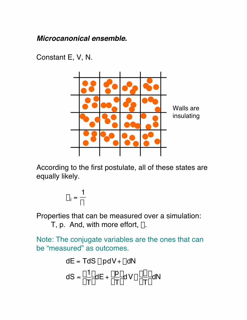
Microcanonical ensemble.

Constant E, V, N.

According to the first postulate, all of these states areequally likely.

p i =1W

Properties that can be measured over a simulation:T, p. And, with more effort, m.

Note: The conjugate variables are the ones that canbe “measured” as outcomes.

dE = TdS - pdV+ mdN

dS =1T

Ê Ë

ˆ ¯ dE +

pT

Ê Ë

ˆ ¯ dV-

mT

Ê Ë

ˆ ¯ dN

Walls areinsulating

Canonical ensemble.

Constant T, V, N.

Now the boxes may have different energies!

Can show (Hill,1986; McQuarrie, 1976) that theprobability of a state is

p i Ei( ) =e-bEi

Q , where b = 1kBT

Properties that can be measured:E, p. And, with more effort, m.

The governing equation isd S -

ET

Ê Ë

ˆ ¯ = -Ed 1

TÊ Ë

ˆ ¯ +

pT

Ê Ë

ˆ ¯ dV-

mT

Ê Ë

ˆ ¯ dN

Walls areconducting

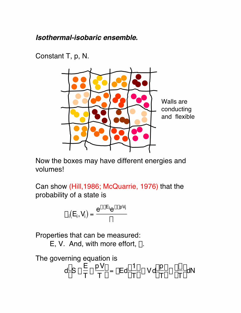
Isothermal-isobaric ensemble.

Constant T, p, N.

Now the boxes may have different energies andvolumes!

Can show (Hill,1986; McQuarrie, 1976) that theprobability of a state is

p i Ei,Vi( ) =e-bEie-bpVi

D

Properties that can be measured:E, V. And, with more effort, m.

The governing equation isd S -

ET -

pVT

Ê Ë

ˆ ¯ = -Ed 1

TÊ Ë

ˆ ¯ - Vd p

TÊ Ë

ˆ ¯ -

mT

Ê Ë

ˆ ¯ dN

Walls areconductingand flexible

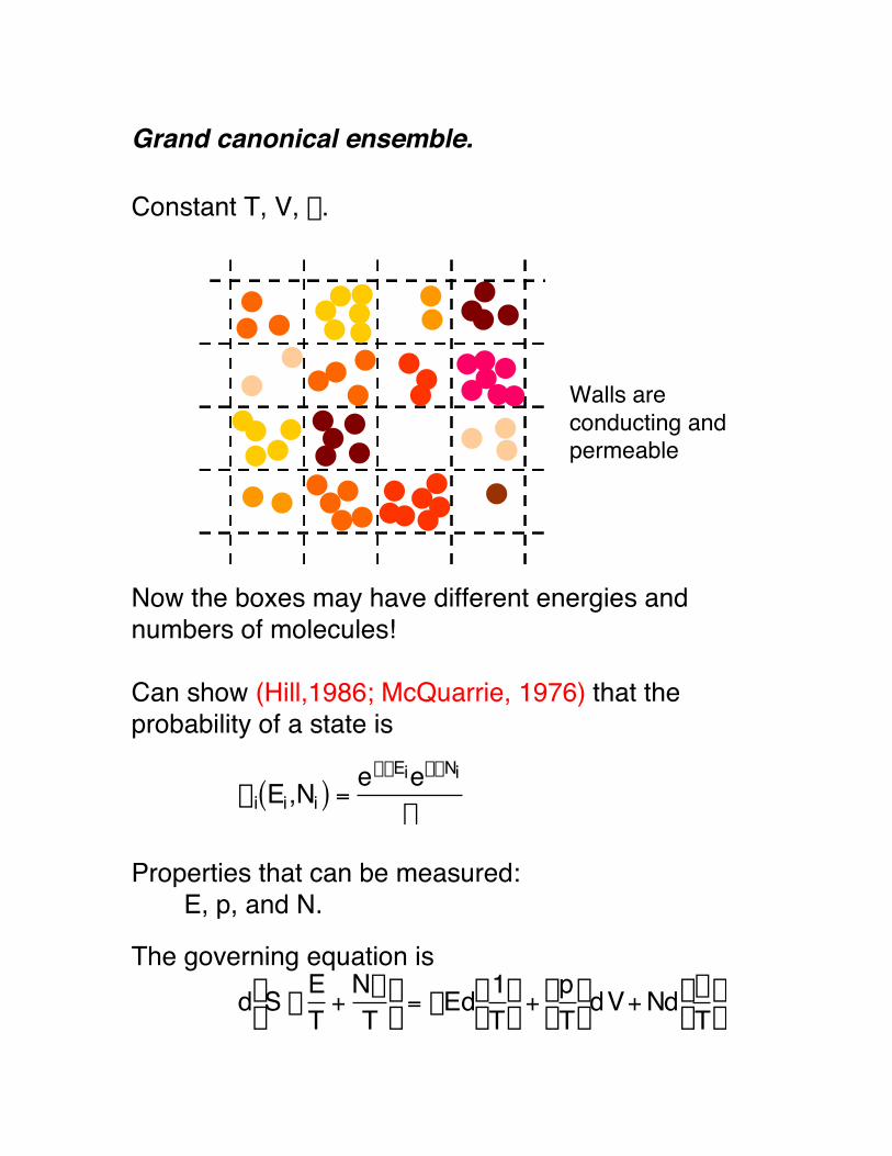
Grand canonical ensemble.

Constant T, V, m.

Now the boxes may have different energies andnumbers of molecules!

Can show (Hill,1986; McQuarrie, 1976) that theprobability of a state is

p i Ei,Ni( ) =e-bEiebmNi

X

Properties that can be measured:E, p, and N.

The governing equation isd S -

ET +

NmT

Ê Ë

ˆ ¯ = -Ed 1

TÊ Ë

ˆ ¯ +

pT

Ê Ë

ˆ ¯ dV+ Nd m

TÊ Ë

ˆ ¯

Walls areconducting andpermeable

Bridges to macroscopic thermodynamics

Partition functions.The normalization constants are referred to aspartition functions, and they have (macroscopic)physical significance.

Summary, in “quantum” notation:

Ensemble PartitionFunction

BridgeEquation

Micro-canonical

W E,V,N( ) = 1i

 SkB

= lnW

Canonical Q T,V,N( ) = e-bEi

i -bA = lnQ

Isothermal-Isobaric

D T,p,N( ) = e-bpV

VÂ e-bEi V( )

iÂ

= e-bpV Q T,V,N( )VÂ

-bG = lnD

Grandcanonical

X T,V,m( ) = ebmN

NÂ e-bEi N( )

iÂ

= ebmN Q T,V,N( )NÂ

bpV = lnX

We can translate these quantum formulas into quasi-classical expressions that are appropriate for ourforce-field-based molecular modeling approach.

Recall that the microstate of a classical system is notdefined by a quantum state, but rather by the positionand momentum of each particle. To get a partitionfunction, we must sum (actually integrate, for theclassical case) over all possible microstates.

Example: canonical partition function

Q =1N!

1h3N ...Ú dp1...dpN dr1...drN e-bHÚ

whereH p N{ },r N{ }( ) = K p N{ }( ) +U r N{ }( )

If we could evaluate this partition function for a modelsystem at various temperatures and volumes, wecould obtain thermodynamic properties via

-bA b,V,N( ) = lnQ

E = -∂ -bA( )

∂b V,N

bp =∂ -bA( )

∂V T,N

However, it is not even close to practical to calculatethe partition function for a typical system.

Example:Say we have a system with N=100 atoms, and wewish to evaluate the configurational (r) part of thecanonical partition function. We have 3N=300coordinates over which to integrate.

Try a Simpson’s rule integration, where 10 functionevaluations per coordinate are employed (a fairlycoarse grid).

# of function evaluations = 10( ) 10( )L 10( ) = 10300

10300operations( ) sec5 ¥ 1012ops

Ê Ë Á

ˆ ¯ ˜ ª 10288 sec

ª 10280yrs

Not likely in the forseeable future!

Instead, we focus on obtaining averages of propertiesof interest.

Formalism for simple averages.One can easily define the average of any propertythat has a simple dependence on the microstatevariables.

For example, in quantum notation

B = Bi pii

Â

In the canonical ensemble, for example, we have

B =Bi e-bEi

iÂ

Q

In classical notation, a similar expression can bewritten for any quantity that has a simple, directfunctional dependence on molecular positions andmomenta.

B =

1N!

1h3N ...Ú dp1...dpN dr1...drN B p{N},r{N}( )e-bHÚ

Q

This seems no better than before – we can’t calculatethe numerator or denominator!

But…

Obtaining simple averages from simulation.Recall that it is the task of a simulation algorithm togenerate microstates in an ensemble, in proportion totheir statistical weights (probabilities).

This can be done- probabilistically (Monte Carlo)- deterministically (molecular dynamics)*

*actually a time average – we’ll revisit this issue

Either way, given a set of nobs representativemicrostates, we can write the average of B as

B =1

nobsB pi

{N},ri{N}( )i=1

nobsÂ

as long as those microstates were generatedaccording to the appropriate weighting function p forthat ensemble!

The quality of the result that you obtain depends onnobs.

Separation of the energy.In the classical limit, the kinetic energy (K) andpotential energy (U) can be considered as separablein the Hamiltonian.

{N}( )

This allows Q to be factored

Q =1N!

1h3N ...Ú dp1...dpN e-bK

Ú( ) ...Ú dr1...drN e-bUÚ( )

and the momentum part will drop out of averages thatdepend only on positions.

B =

1N!

1h3N ...Ú dp1...dpN e-bKÚ( ) ...Ú dr1...drN B r{N}( )e-bUÚ( )1N!

1h3N ...Ú dp1...dpN e-bK

Ú( ) ...Ú dr1...drN e-bUÚ( )

=...Ú dr1...drN B r{N}( )e-bUÚ

...Ú dr1...drN e-bUÚ

This is why Monte Carlo, where there is no time, canstill be useful in obtaining thermodynamic properties.

Examples of simple averages.

Kinetic energy.

The classical definition is

K =1

2mipi

2

i=1

NÂ

So we have

K =1

nobsK pi

{N}( )i=1

nobs =

1nobs

12mi

pi2

i=1

NÂ

Ê

Ë Á

ˆ

¯ ˜

i=1

nobsÂ

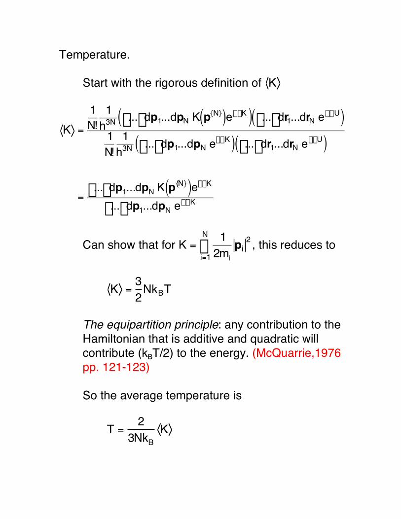
Temperature.

Start with the rigorous definition of K

K =

1N!

1h3N ...Ú dp1...dpN K p{N}( )e-bKÚ( ) ...Ú dr1...drN e-bUÚ( )

1N!

1h3N ...Ú dp1...dpN e-bK

Ú( ) ...Ú dr1...drN e-bUÚ( )

=...Ú dp1...dpN K p{N}( )e-bKÚ

...Ú dp1...dpN e-bKÚ

Can show that for K =1

2mipi

2

i=1

NÂ , this reduces to

K =32NkBT

The equipartition principle: any contribution to theHamiltonian that is additive and quadratic willcontribute (kBT/2) to the energy. (McQuarrie,1976pp. 121-123)

So the average temperature is

T =2

3NkBK

Potential energy.

This is simply the interaction potential within andbetween molecules (intramolecular andintermolecular, respectively). It depends only onthe atomic coordinates, not the momenta.

So we may write

U =1

nobsU ri{N}( )

i=1

nobsÂ

We may write a similar relationship for anyparticular component of the potential energy. Forexample, for a polymeric system we may beinterested in the torsional component of thepotential:

Utors =1

nobsUtors ri{N}( )

i=1

nobsÂ

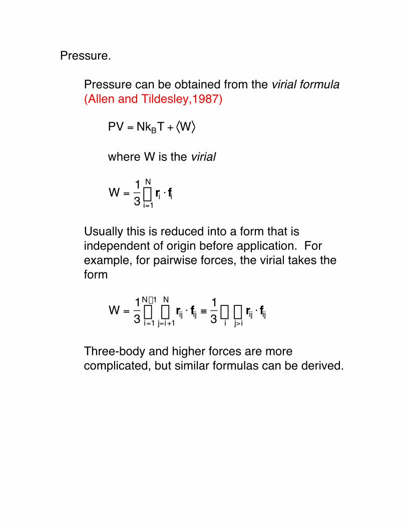
Pressure.

Pressure can be obtained from the virial formula(Allen and Tildesley,1987)

PV = NkBT + W

where W is the virial

W =13 ri ⋅ fi

i=1

NÂ

Usually this is reduced into a form that isindependent of origin before application. Forexample, for pairwise forces, the virial takes theform

W =13 rij ⋅ fij

j=i+1

NÂ

i=1

N-1Â ≡

13 rij ⋅ fij

j>iÂ

iÂ

Three-body and higher forces are morecomplicated, but similar formulas can be derived.

Chemical potential.

Chemical potential is not a “mechanical variable”– it does not have a “simple, direct functionaldependence on molecular positions andmomenta.”

Calculating the chemical potential of a speciesfrom a molecular simulation can be quitechallenging; we will discuss this in detail later.

For now, the following definition (in the canonicalensemble) provides a clue on how it might becalculated

bm = -∂ -bA( )

∂N b,V

Ergodicity

Ergodic hypothesis.“…a large number of observations made on a singlesystem at n arbitrary instants of time have the samestatistical properties as observing n arbitrarily chosensystems at the same time from an ensemble…”(McQuarrie,1976)

time average Û ensemble average

We believe that it “holds for all many-body systems innature.” (Chandler,1987)

Implications for molecular simulation.(Allen and Tildesley,1987; Frenkel and Smit,1996)

molecular dynamicssimulation in timeaverage over snapshots in time

Monte Carloprobabilistic walk through configurationsaverage over (properly weighted) configurations

When we simulate a given model system under agiven set of macroscopic constraints, we should getstatistically identical results from MD and MC.

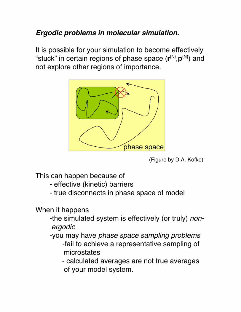
Ergodic problems in molecular simulation.

It is possible for your simulation to become effectively“stuck” in certain regions of phase space (r{N},p{N}) andnot explore other regions of importance.

(Figure by D.A. Kofke)

This can happen because of- effective (kinetic) barriers- true disconnects in phase space of model

When it happens-the simulated system is effectively (or truly) non-ergodic-you may have phase space sampling problems

-fail to achieve a representative sampling ofmicrostates- calculated averages are not true averagesof your model system.

phase space

Phase-space sampling problems can occur with bothMD and MC algorithms. There are several ways tolook for, and avoid, such problems.

Molecular dynamics- increase simulation time- vary starting conditions- use annealing

Monte Carlo- same remedies as MD, plus…- use special (bolder) algorithms

Role of simulation, re-visited

For a given model system, the tasks of a molecularsimulation are to:

(1) Sample microstates within an ensemble, with theappropriate statistical weights

(2) During the sampling, calculate and collectmolecular-level information that aids in understandingthe physical behavior of the system

(3) Employ a large enough sample size to ensure thatthe collected information is meaningful(Note: even with today’s powerful computers, it isgenerally impossible to sample all of the microstatesof a model system.)