brussels, 04 october 2006 - cnr · introduction to the dtu wind energy research fields ......
TRANSCRIPT

SCIENTIFIC REPORT
ACTION: ES1303 TOPROF
STSM: COST-STSM-ES1303-30536
TOPIC: Validation of real time turbulence estimation and measurement of
wind gust using Doppler lidar.
VENUE: Technical University of Denmark (DTU), Risø Roskilde Denmark
PERIOD: 18 January – 05 february 2016
Host: Sven-Erik Gryning (DTU Wind Energy, Denmark)
Applicant: Lucie Rottner (Météo-France, CNRM, France)
Submission date: 18.02.2016
Contribution by: Lucie Rottner (Météo-France, CNRM, France), Irene
Suomi (Finnish Meteorological Institute, Finland)
1

Introduction
A preliminary work on a new way to estimate atmospheric turbulence using
high-frequency Doppler Lidar measurements has been recently achieved by
Christophe Baehr (Météo-France, CNRM, Toulouse, France) and myself. The
turbulence estimations are based on wind reconstruction using Lidar WindCube
observations and a particle filter (Rottner L, Baehr C., 2014). The suggested
reconstruction algorithm links the WindCube observations to numerical particles to
obtain turbulence estimations every time new observations are available. The high
frequency of the estimations is a new point which has to be validated (figure 1).
Moreover, the presented algorithm enables to reconstruct the wind in three
dimensions in the observed volume. We have thus locally access to the spatial
variability of the turbulent atmosphere.
The suggested algorithm has already been applied to a reduced set of real
observations. The obtained results are very encouraging : they show significant
improvements on turbulent parameter estimations. The objective is now to validate the
reconstruction algorithm using longer data sets (from one week to one month).
2
Figure 0: WindCube lidar with an illustration of the five lines of sight (left), an example
of particles within the volume of the particle filter (middle) and an example of the TKE
calculated from the particle velocities (red curve) and from the reference
measurements (black stairs) (right).

As an advanced research center on wind energy, the DTU gathers all the
equipment and human expertise which are required to validate the reconstruction
algorithm. For instance, several Doppler lidars are operated in Høvsøre at the foot of a
high meteorological mast equipped with sonic anemometers. Besides, members of the
DTU Wind Energy are world specialists of turbulence measurements.
The scientific mission has been the opportunity to get several data sets of lidar
observations, and to set the basis of a collaborative work with Irene Suomi on wind
gusts.
Objectives
The main objectives of the STSM were :
Introduction to the DTU Wind Energy research fields
Presentation of the turbulence estimation method, and presentation of results
previously obtained
Definition of the policy of use of the DTU data
Downloading WindCube V2 data and anemometer data from the Høvsøre site
Application of the reconstruction method to the DTU data
Introduction to wind gusts measurements (Irene Suomi)
Definition of the frame work with Irene Suomi : real time parameter required,
number of cases to study, data format
Performing the first test experiments to begin the work on the relationship
between wind gusts and turbulent parameters
Presentation of the first results
Results or Achievements
Observation data sets and validation of 3D wind reconstruction and
turbulence estimation method
The aim of the STSM was to get long data sets of WindCube V2
measurements. These data sets will then be used to validate the new method of
turbulence estimation. The method gives access to turbulent parameters in real time :
it is the innovative point which has to be validated.
3

During the STSM, I have downloaded three kinds of wind observations from the
DTU database. The observations come from the Høvsøre test center for large wind
turbines (figure 2). The site has been described in details by Peña et al. (2015). First,
WindCube V2 measurements have been downloaded. These observations are
available at a frequency of 0.25Hz. Secondly, sonic anemometer measurements have
been downloaded. The observations are available at different heights from 10m to
116m, at a frequency of 20Hz. The sonic data will be useful to validate the real time
turbulence estimations given by the reconstruction algorithm. Then I have downloaded
cup anemometer data and wind vane data averaged over 10 minutes. These data will
be used to assess the estimation of wind direction and of turbulent intensity.
4
Figure 2: The Danish National Test Station for Large Wind Turbines is located at
Høvsøre, at the western coast of Denmark (left). The 116.5 m tall meteorological mast is
situated at left on the right hand side picture.

The downloaded data are resumed in the following table :
Date Instruments
01-31/05/2013 Windcube V2 unit 139, sonic anemometer, 10min data
01-05/06/2013 Windcube V2 unit 139, sonic anemometer, 10min data
08-31/07/2013 Windcube V2 unit 139, sonic anemometer, 10min data
01-31/08/2013 Windcube V2 unit 139, sonic anemometer, 10min data
01-31/08/2013 Windcube V2 unit 139, sonic anemometer, 10min data
01-31/12/2013 Sonic anemometer, 10min data
01-05/12/2013 Windcube V2 unit 62
06-13/12/2013 Windcube V2 unit 62
01-31/01/2014 Windcube V2 unit 62, sonic anemometer, 10min data
01-28/02/2014 Windcube V2 unit 62, sonic anemometer, 10min data
01-31/10/2015 Windcube V2 unit 139, sonic anemometer, 10min data
The data from the DTU database have been formatted to be easily used by the
reconstruction method. Then the first step of the validation work has begun. The
reconstruction method has been applied to 2 hours of WindCube observations. The
preliminary results I have obtained show the capability of the reconstruction method to
estimate 3D wind and turbulence. The results are presented in the following
paragraphs.
To validate the reconstruction method, the first point is to validate the 3D wind
reconstruction. On figure 3, 30 minutes time series of the reconstructed wind and of
the WindCube V2 wind are shown. We can notice that the time series are in very good
agreement when the WindCube observations are fine. For the meridian wind (V) and
for the vertical wind (W) there is a spike in the WindCube time series. It is linked to a
transient measurement error. We can notice that the reconstruction method is able to
remove the spike and to reconstruct coherent time series.
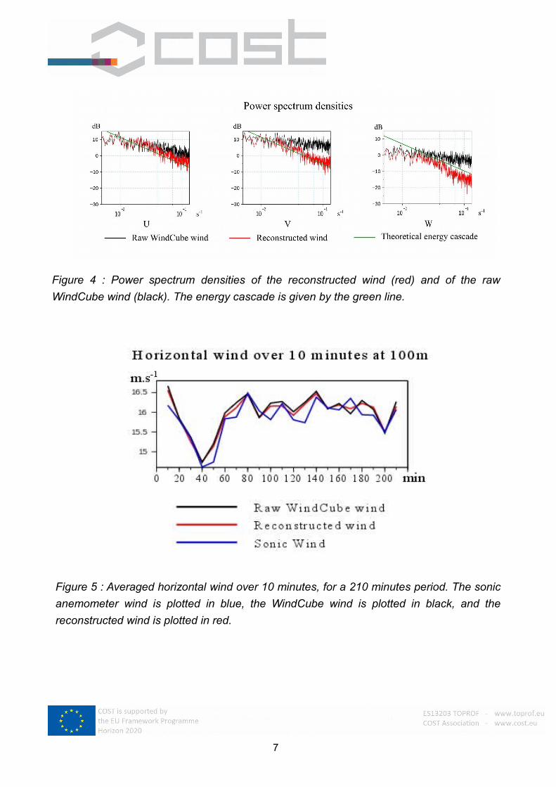
On figure 4 the power spectrum densities of the reconstructed wind and of the
WindCube V2 wind are represented. The power spectrum densities are compared to
the theoretical energy cascade. This cascade describes the energy transfer from large
scales to small scales in the atmosphere. The figure 4 shows that the WindCube
observations follow the energy cascade for the zonal wind (U) only. The power
spectrum densities of the two other components are almost flat. It reflects that the
5

WindCube retrieves noisy wind observations. On the contrary, the slopes of the power
spectrum densities of the reconstructed wind follow the energy cascade.
The horizontal WindCube wind and the horizontal reconstructed wind have also
been compared to sonic anemometer measurements. Figure 5 represents the
horizontal winds averaged over 10 minutes, for a 210 minutes period. The figure
shows a good agreement between the averaged winds.
The study of the reconstructed wind has shown that the reconstruction method is
able to filter spikes in the time series. In addition, starting from noisy observations, the
method retrieves 3D wind in good agreement both with sonic data and with the
turbulence laws in the atmosphere.
6
Figure 3 : Time series of the three components of the wind over 30 minutes from 4 pm,
10/06/2015. The raw WindCube wind is plotted in black, and the reconstructed wind is
plotted in red.
7
Figure 4 : Power spectrum densities of the reconstructed wind (red) and of the raw
WindCube wind (black). The energy cascade is given by the green line.
Figure 5 : Averaged horizontal wind over 10 minutes, for a 210 minutes period. The sonic
anemometer wind is plotted in blue, the WindCube wind is plotted in black, and the
reconstructed wind is plotted in red.
Having validated the reconstructed wind, I have worked on the turbulent intensity.
The turbulent intensity is an important parameter to design wind turbines. Indeed, the
turbines are calibrated for a specific range of turbulent intensity. To measure the
turbulent intensity, cup anemometers are the reference instruments. By comparison
with cup anemometers, the lidar WindCube V2 is known to overestimate the turbulent
intensity. Previous results have shown that the reconstruction method retrieves good
estimation of the turbulent intensity. The data downloaded from the DTU database will
be used to assess this point.
On figure 6 the vertical profiles of turbulent intensity obtained from the WindCube
V2 data and from the reconstructed method are represented. We can notice that the
reconstructed turbulent intensity is lower than the WindCube turbulent intensity.
However, the two profiles show the same temporal evolution. The objective will be to
compare the turbulent intensity calculated over several days from the WindCube data,
8
Figure 6 : Vertical profiles of turbulent intensity from the raw WindCube data (upper part)
and from the reconstructed wind (lower part).

from the reconstructed wind, from the sonic anemometer data and from the cup
anemometer data.
Measurement of wind gusts using Doppler lidar (with Irene Suomi)
This work is done in collaboration with Irene Suomi. The aim is to study the
dependence of wind gusts on turbulence measurements using the reconstruction
method. The objective is to study the link between the turbulent intensity, or the
turbulent kinetic energy -calculated in real time using the reconstruction method- and
the wind gusts. Besides, among the outlines, there is the issue of the extension of the
surface gust measurements throughout the boundary layer. During the STSM, a new
question has also been raised : can we use the statistical characteristics of the particle
system used in the reconstruction method to retrieve the extreme wind values
measured by sonic anemometers ?
This work has begun by a presentation about wind gusts (Suomi et al., 2015).
Then Irene Suomi and I have first defined the ideal cases which would be selected.
According to the geography of the Høvsøre test site, only easterly strong winds should
be chosen for gust study. To be in the optimal working range of the reconstruction
method, we have to choose periods when the turbulence is the more developed. Thus
data from 10 am to 6 pm should be selected. In October 2015, winds were mainly
easterly at Høvsøre. In addition, the 10/06/2015 horizontal winds higher than 16m/s
have been observed during the afternoon. We have thus decide to begin our study
with this case. A first work on wind gust has already been done.
In this premilinary study, we investigate how information about the particle
velocities could be used in the derivation of a gust estimate. Figure 7 shows the first
results of such analysis. At first, the data was divided into 10 min bins. The mean
horizontal wind speeds calculated from the reference sonic anemometer, directly from
the original lidar measurements and from the reconstructed wind speed agree well
(the dashed lines on figure 7). The wind speed maxima, i.e. the gusts, were calculated
from sonic anemometers by applying a 3.8 s moving average to the measured 20Hz
wind speed signal and the gust was determined as the maximum of each 10 min
period of the signal. The length of the moving average window, 3.8 s, was chosen to
be the same as the time taken for a lidar to measure a full set of five beams, i.e. it is
the resolution of the lidar measurements (as well as of the reconstructed velocity).
On figure 7, the wind gust speed of the reconstructed wind agrees well with the
sonic anemometer gusts of 3.8 s duration, but the original lidar wind speed maxima
are slightly higher than the sonic ones. Figure 7 also shows that the unrealistically
9

high maximum in the lidar wind gust speed centered at 85 min is efficiently removed
by the reconstruction method.
On figure 7, the maxima of the sonic anemometer data (Umax,sonic, the raw 20Hz
measurements) are clearly higher than the ones derived from the original or
reconstructed lidar measurements. One possibility to estimate the wind gust is to take
the maximum of the particle velocities as the gust estimate. However, in this case it
leads to unrealistically large wind speed maxima. However, potentially the information
about the particle velocity distributions within the turbulence model could be used to fill
the gap between the lidar maxima and the maxima of the raw sonic anemometer
signals.
Designing new experiences to work on wind gust measurements
During the STSM and to support it, DTU started another lidar measurement
campaign at the National Test Centre for Large Wind Turbines at Østerild (57° 3' 0.27"
N, 8° 52' 55.70" E) which is located north of Høvsøre. The advantage of this site is
that there is a 250 m high, extensively instrumented meteorological mast, which will
provide good quality reference measurements from sonic anemometers at heights 8,
40, 103, 175 and 241 m (figure 8). Since the 25/01/2016, a WindCube V2 has been
calibrated to measure winds at 40m, 70m, 103m, 106m, 140m, 175m, 178m, 210m,
241m, 244m, 270m and 290m. The data from this site will be used to complete the
gust study that will be done with the data from Høvsøre. For the comparison with
anemometer data, we have to remind that the lidar has an offset from North of
52.5deg.
10
Figure 7 : Mean wind (U) and wind gust (Umax) speed calculated from the original lidar,
reconstructed lidar (red) and sonic anemometer meausrements. For the latter, Umax is
calculated as the maximum of 3.8 s moving averages and as the maximum of the original raw
(20 Hz) signal.

11
Figure 8 : Meteorological mast at Østerild. Cup anemometers, sonic anemometers
and wind vanes are hanged at different heights. The WindCube V2 has been
calibrated to measure wind at the same heights.

Conclusions
The scientific mission has given me the opportunity to get several data sets of
lidar observations. I have also presented and discussed the reconstruction algorithm
with experts on turbulence measurement using Doppler lidar. Moreover, Irene Suomi
and I have begun a new work on wind gust. The basis of this collaborative work has
been set, and we except to obtain innovative results in the next few months. To
conclude, as all the objectives have been been met and exceeded, and as an
interesting work on wind gust measurements in collaboration with Irene Suomi has
begun, this STSM was a successful mission.
Deliverables
As an outcome of this STSM an abstract was submitted to the 22nd Symposium on
Boundary Layers and Turbulence, which will be held in Salt Lake City, Utah, USA
during 20–24 June 2016 (Suomi et al., 2016). Another abstract related to turbulence
estimation will also be submitted before the end of February 2016 to the International
Symposium for the Advancement of Boundary Layer Remote Sensing (Rottner et al.,
2016).
References
Peña A, Floors R, Sathe A, Gryning S-E, Wagner R, Courtney M S, Larsen X G, Hahmann A
N, Hasager C B. 2015. Ten years of boundary-layer and wind-power meteorology at
Høvsøre, Denmark. Boundary-Layer Meteorol. doi: 10.1007/s10546-015-0079-8.
Rottner L, Baehr C. 2014. 3D Wind Reconstruction and Turbulence Estimation in the
Boundary Layer from Doppler Lidar Measurements using Particle Method. AGU Fall Meeting
Abstracts, http://adsabs.harvard.edu/abs/2014AGUFMNG23B3806R
Rottner L, Suomi I, Rieutord T, Baehr C, Gryning S-E. 2016. Real time turbulence and wind
gust estimation from wind lidar observations using the turbulence reconstruction method. 18 th
International Symposium for the Advancement of Boundary Layer Remote Sensing, 6-9 June
2016.
Suomi I, Gryning S-E, Floors R, Vihma T, Fortelius C. 2015. On the vertical structure of wind
gusts. Q.J. R. Meteorol. Soc. 141: 1658-1670. doi:10.1002/qj.2468.
Suomi I, Rottner-Peyrat L, O'Connor E, Gryning S-E, Sathe A. 2016. Wind gust
measurements using pulsed Doppler wind-lidar: comparison of direct and indirect techniques.
22nd Symposium on Boundary Layers and Turbulence, 20–24 June 2016, American
Meteorological Society, Salt Lake City, Utah, USA. (submitted).
12