bsg 2012 14 (bsg lessons from the 2011 european stress tests exercise)
TRANSCRIPT

Do Stress Tests reduce Bank Opaqueness? Lessons from the 2011 European Exercise
Giovanni Petrella* and Andrea Resti**
December 5, 2011 – DRAFT – COMMENTS WELCOME
Abstract - Supervisory stress tests assess the impact of an adverse macroeconomic scenario on the profitability and capitalisation of a large number of banks (accounting for a significant share of the overall loans and deposits). The results of such stress test exercises have recently been disclosed to the public in an attempt to restore confidence by curbing bank opaqueness, i.e., helping investors distinguish between sound and fragile institutions. The 2011 European Union stress test carried out by the EBA lead to the release of some 3,400 data points for each of the 90 participating banks. Market participants were not only given a predetermined, "black box" outcome, but were also in a position to adjust the supervisors’ “adverse scenario” by simulating further shocks and to assess each bank’s resilience to alternative assumptions. This makes the 2011 EU exercise an ideal empirical experiment to investigate a number of hypotheses on stress tests and bank opaqueness. E.g., were the test’s results deemed relevant by investors or simply ignored? Did they trigger a price adjustment process, and if so, for what banks? To what variables did the market associate the strongest importance? Did investors care about the results of the EBA’s adverse scenario, or did they simply rely on historical, detailed data to run their own stressed simulations? The paper investigates such questions through a thorough econometric analysis of stock-market data.
1 Introduction
A supervisory “stress test” program requires a large number of banks (accounting for a
significant share of the overall loans and deposits) to assess the impact, on their
profitability and capitalisation levels, of an adverse macroeconomic scenario.
Unlike in the internal stress tests used by individual banks for risk management and capital
planning purposes (and required by the so-called “Pillar Two” in the 2004 Basel Accord),
supervisory stress tests are to be run by all involved institutions based on the same
downturn scenario (e.g., a 2% decrease in GDP, a 3% surge in the unemployment rate, a
20% drop in stock prices, etc.) and covering an identical forecast window (typically two
years). This makes supervisory stress test results highly comparable across banks.
The outcome of the test can be kept confidential by the supervisors, but recently results
have often been disclosed to the public, in an attempt to restore confidence and help
investors distinguish between sound and weak institutions (with the latter often being
forced to recapitalise as the stress test results were announced).
* Università Cattolica del Sacro Cuore, Milano ([email protected]); ** Bocconi University,
Milano ([email protected]). Helpful comments by Mario Quagliariello are gratefully acknowledged.

Do Stress Tests reduce Bank Opaqueness? Lessons from the 2011 European Exercise
* 2 *
It has been argued, however, that such publicly disclosed stress tests are inherently flawed:
on one side, supervisors cannot test adverse scenarios which are extreme enough to provide
a truly “stressed” environment, as they might scare investors or simply be politically
unpalatable (e.g., scenarios involving the default of one or more sovereign entities); on the
other hand, if the downturn scenarios are perceived as too mild by investors, the stress test
results will simply be ignored by market participants. Also, if macroeconomic conditions in
the following months deteriorate more than it was anticipated by the “stressed”
assumptions (possibly leading to the failure of one or more banks which had passed the
test), this might dent the supervisors’ credibility and hence lead to greater market
uncertainty1.
To address such concerns, some supervisors have decided not to disclose the stress test
results, using them only internally, as a way to pre-emptively address capital shortages by
individual banks. Furthermore, even those supervisors who still make results public are
increasingly shifting away from issuing a simple, “binary” signal on “pass” and “fail”
banks, and have considerably increased the depth and width of the data released to the
public, to help investors “decide for themselves”, based on fresh, rich, reliable data.
Namely the 2011 European Union stress test (carried out by the European Banking
Authority, EBA) lead to the release of some 3,400 data points for each of the 90
participating banks. As all banks had to use the same data structure (which was shared with
the public ahead of the results’ publication), market participants were in a position to adjust
the supervisors’ “adverse scenario” by simulating further shocks and assessing each bank’s
resilience to alternative sets of assumptions.
This makes the 2011 EBA stress tests an ideal empirical experiment to investigate a
number of hypotheses on stress tests and bank opaqueness. Were the test’s results deemed
relevant by investors or simply ignored? Did they trigger a price adjustment process, and if
so, for what banks? To what variables did the market attach the strongest importance? Did
1 Furthermore, some banks have argued that, if too many details on balance-sheet composition are made
public, this could damage business confidentiality and give rise to legal risks. Also, other market participants could gain insights into one bank’s risk profile, e.g. by estimating the amount of needed financial hedges and using this information to carry out arbitrage strategies on the CDS market (Bryant 2011).

Do Stress Tests reduce Bank Opaqueness? Lessons from the 2011 European Exercise
* 3 *
investors care about the results of the EBA’s adverse scenario, or did they simply rely on
newly-available detailed data to run their own stressed simulations?
Another fact that makes the 2011 EU stress test an interesting area of research is that it was
quickly dismissed by some bank analysts as plainly useless, as it failed to reverse the
downward trend experienced by bank stock prices in late 2010 and 2011. Such conclusions
appear somewhat rushed. One one hand, it is hard to see how a supervisory exercise, no
matter how timely and accurate, could by itself stop a long-lasting decline in bank shares
and prevail over market jitters caused by a deep sovereign debt crisis. On the other hand,
stress tests cannot be evaluated by looking at market returns in the following weeks or
months, as they are most likely affected by a number of further news and events (e.g.,
bailout plans for Greece) which go well beyond the stress test exercise. Accordingly, a
rigorous econometric analysis is needed, focusing on the days immediately after the release
of stress test results, before one can claim that the whole exercise was ineffective.
This paper unfolds as follows: §2 summarises previous research results on bank
opaqueness and stress tests; §3 presents the main features of the 2011 European stress test;
§4 states the hypotheses to be tested in our empirical analysis; §5 describes our sample,
methodology and key variables; §6 shows our main results, while further results and
robustness checks are presented in §7; §8 concludes.
2 Literature review
Compared to other companies, banks have an higher share of assets which suffer from a
strong degree of opaqueness: e.g., loans are informationally sensitive and hard to evaluate
for outsiders, while liquid assets are easily sold and replaced, so that the data in financial
statements may rapidly become obsolete. As a result, banks may be harder to assess, for
investors and rating agencies, than non-bank companies.
A proof of bank opacity is the fact that market prices react to supervisory announcements
(Jordan 2000). Also, split ratings tend to occur more often for banks than for non-bank
companies (Morgan 2002; Iannotta 2006), suggesting that the latter are harder to assess,
due to stronger opaqueness. Regressions of bank stock returns on market indices show

Do Stress Tests reduce Bank Opaqueness? Lessons from the 2011 European Exercise
* 4 *
higher R-squares (Haggard and Howe 2007); this means that firm-specific information is
harder to extract and therefore plays a less relevant role for bank stock prices2.
Several supervisory tools are usually put in place, including deposit insurance and risk-
based capital requirements, to prevent lenders and depositors from being scared away by
bank opacity. As opacity tends to increase in times of crisis (Flannery, Kwan, and
Nimalendran 2010), additional instruments are needed to reassure the market during a
financial turmoil.
This is the case of the stress testing exercises carried out in the US (20093) and the
European Union (20104 and 20115). The effects of a downturn scenario on a large number
of banks were simulated, with the main results being released to the public (including any
capital shortfalls arising from the simulation). By disclosing information on each bank’s
strengths and vulnerabilities, the supervisors aimed at reducing market uncertainty,
stabilise stock prices and prevent panic6; the idea was that investors, when presented with a
deep and robust flow of data (made comparable across banks and somewhat “certified” by
the supervisors’ intervention in the test), would consider banks less opaque, and therefore
better differentiate among banks when setting the risk premium required to invest in equity
capital, or to lend.
Table 2 illustrates the main characteristics of the three exercises mentioned above7,
highlighting the amount of information released to investors. While the 2009 and 2010
stress tests implied the publication of a limited number of key figures for each bank, the
2011 EU-wide test was significantly more ambitious, as more than 3,400 data-points for
each bank could, in principle, be provided8.
2 The fact that bank prices are driven mostly by easily observable variables (like market indices) also
provides an explanation for the results in (Flannery, Kwan, and Nimalendran 2004), where stockmarket analysts are found to agree more often on bank valuations than they do for other industries.
3 (Federal Reserve 2009a). 4 (Committee of European Banking Supervisors 2010). 5 (European Banking Authority 2011a). 6 To quote the Federal Reserve report whereby the 2009 stress test results were released to the public, “the
decision to depart from the standard practice of keeping examination information confidential stemmed from the belief that greater clarity […] will make the exercise more effective at reducing uncertainty and restoring confidence in our financial institutions” (Federal Reserve 2009b).
7 Stress testing exercises have also been carried out, with different scope and depth, by most national authorities in the European Union. See (Quagliariello 2009) for a complete picture of macro- and micro- stress testing approaches in many European countries.
8 This included a breakdown of sovereign bonds and credit exposures by country and duration bands; as most banks did not have an exposure to all countries and duration bands, many data points (about 73% of the total) were filled with zeroes; note however that those were meaningful zeroes, informing that a given

Do Stress Tests reduce Bank Opaqueness? Lessons from the 2011 European Exercise
* 5 *
Table 1: Main Stress Test Exercises in the US and EU
Exercise Announcement date
Results release
date
Banks covered # of released data items per bank
Minimum capital
target(s)
Capital shortfalls
found
Supervisory Capital Assessment Program (SCAP) by Federal Reserve, FDIC, OCC, OTS
February 10, 2009
May 7, 2009
19 domestic bank holding companies covering 2/3 of
the assets in the US banking system
17 Common Tier 1 at 4%, Tier
1 at 6%
10 banks, USD 75 bn.
2010 EU-wide Stress Testing Exercise by the Committee of European Banking Supervisors
December 2, 2009
July 23, 2010
91 banks, covering 65% of the assets in the EU
banking system and at least 50% for each member
country
27 Tier 1 at 6% 7 banks (+17 “near fail”),
€3.5 bn.
2011 EU-wide Stress Test by the European Banking Authority
January 12, 2011
July 15, 2011
90 banks, covering 65% of the assets in the EU
banking system and at least 50% for each member country
3,456 Core Tier 1 at 5%
8 banks (+16 “near fail”),
€2.5 bn.
These stress tests and their market impact have been discussed by some recent research
papers. (Hirtle, Schuermann, and Stiroh 2009) provide a qualitative assessment of how the
2009 US exercise (the “SCAP”) was received by investors: in the Authors’ opinion, the
process was perceived as rigorous and thorough, transparency was appreciated, the
aggregate estimated capital shortfall was seen as reasonable and consistent with other
analysts’ forecasts, the variation across firms was in line with market expectations. In
short, the SCAP was appreciated by the market because it did not add any major
unforeseen element to the market’s information set; paradoxically, one might say that it
helped reassure markets right because it did not significantly increase transparency9.
A more quantitative assessment of the SCAP’s market impact is provided by (Peristiani,
Morgan, and Savino 2010) using standard event study models. Several dates are analysed,
including the SCAP’s initial announcement, the release of some important clarifications
regarding its methodology and policy implications (in terms of compulsory capital
increases and possible government interventions), and of course the final disclosure of
bank-by-bank figures. The market is found to have reacted only to policy-related
bank was not exposed to that specific combination of duration and nationality. Another 5.3% of the data points included missing values; again most of them were, again, “meaningful missings”, e.g. to indicate that banks did not expect any state aid in the following months, neither through equity nor hybrid securities.
9 In the Authors’ words, “whether the reception would have been positive if […] there had been a negative “surprise” about a firm or a group of firms, remains open to debate”.

Do Stress Tests reduce Bank Opaqueness? Lessons from the 2011 European Exercise
* 6 *
clarifications and to the publication of stress test results. Investors have been able to guess
in advance what banks would be required to raise extra capital; accordingly, when actual
results were released, the impact on stock prices was not driven by the “gross” capital
shortfall highlighted for each bank, but rather by its “unanticipated” component (net of
market expectations). Overall, the stress test exercise appears to have been informative to
investors, hence to have had a positive effect in terms of dissipating opaqueness and relieve
panic.
(Blundell-Wignall and Slovik 2010) look at the 2010 EU-wide stress test with a special
focus on the treatment of sovereign debt. In the 2010 simulation, government bonds were
subject to a haircut only when held in the trading portfolio (while no credit-related losses
were imposed on sovereign exposures in the banking book10). The Authors show that 83%
of the sovereign debt held by EU banks at end 2009 was instead held in the banking book,
and conclude that this could explain why the encouraging results of the 2010 stress test
failed to reassure the market. To some extent, their critique also applies to the 2011
exercise, as again no proper haircut was imposed on sovereign bonds outside the trading
book; however, the credibility of the final results was somewhat improved by the fact that
losses were imposed also on sovereign exposures held in the banking book, although
indirectly (through a floor on the “expected loss rate” applied to exposures towards banks
and sovereigns located in different countries, see Appendix 1 for details).
(Beltratti 2011) looks at the 2011 EU-wide stress test and concludes that they provides
relevant information to markets, since their outcome (i.e., the capital shortfall associated
with individual banks) could not be forecast by combining variables that were already
known to the market ahead of the stress test exercise.
(Cardinali and Nordmark 2011) analyse the 2010 and 2011 European stress tests by
looking at cumulative abnormal returns for tested and untested banks. However, they not
cover the release of 2011 results, but only the announcement of the new stress test and a
number of methodological clarifications issued by the European Banking Authority while
data were being collected and processed. While the 2010 exercise appears to have been
relatively uninformative to investors, the release of the 2011 methodology (including the
10 Loosely speaking the trading portfolio, or trading book, consists of financial assets held at fair value and
includes the bank’s own position in financial instruments for trading purposes (ie., aimed at generating profits in the short run by buying and selling securities) as well as derivatives held to hedge that position. The banking book includes all other exposures (often long term) which are not held in the trading book.
Do Stress Tests reduce Bank Opaqueness? Lessons from the 2011 European Exercise
* 7 *
decision to focus on a “core Tier 1” target11 of 5% which was considerably more
conservative than the one used one year before) gave rise to negative CARs for stress-
tested banks, while non-tested institutions remained roughly unaffected. Also, the paper
finds no major differences between PIIGS and non-PIIGS banks12.
3 The 2011 EU-wide stress test
3.1 Scope and assumptions
The 2011 EU-wide stress test was carried out on 90 banks accounting for more than 65%
of the total assets in the EU banking system. For each member state, a variable number of
banks were included, starting from the largest one and stopping when at least 50% of total
assets was covered13.
The starting point was the financial data as of December 31, 2010. The simulation exercise
covered two years (2011 and 2012) and consisted of two scenarios: baseline (designed by
the European Commission) and adverse (set up by the ECB).
Under the baseline scenario a strengthening of macroeconomic recovery was assumed,
with GDP growth of 1.7% and 2% in the EU. Under the adverse scenario, GDP would
shrink by 0.4% in 2011 and stay flat in 2012; meanwhile, equity prices would drop by
15%, short-term risk-free rates would increase by 1.40% and long-term ones by 1.25%.
Credit spreads for sovereign debts in Europe would also pick-up, with different increases
for individual countries. The USD would devaluate by 11%.
Starting from such macroeconomic assumptions, banks were requested to use their internal
models to generate values for balance-sheet items and P&L results. In doing so, however,
they had to follow a detailed methodology specified by EBA. Firm-specific assumptions,
as well as results generated by individual banks, were subsequently cross-checked by
national supervisors and by EBA itself, and further calibrated when necessary.
11 “Core Tier 1” refers to high-quality capital, such as common equity and government-sponsored hybrid
securities, net of a number of deductions to make the final result robust and comparable across different banks and countries. However, it is not equivalent to the “common equity Tier 1” capital dictated by the so-called “Basel 3” agreement.
12 PIIGS banks are those headquartered in Portugal, Ireland, Italy, Greece and Spain. 13 National authorities could add further banks in sample, beyond this minimum requirement (e.g., Spain
included several other minor banks).

Do Stress Tests reduce Bank Opaqueness? Lessons from the 2011 European Exercise
3.2 Key dates
As shown in Figure 1, the stress test was announced by EBA on 13 January 2011 (“the first
announcement date”) with a short press release highlighting the expected duration of the
exercise (“first half of 2011”) and EBA’s commitment to make results public14. No further
details were provided.
On 2 March 2011 (“the detailed announcement date”) EBA outlined the overall logic
underlying the simulation exercise and indicated that EU member states might put in place
“remedial back stop measures” (i.e., capital increases) to address any weaknesses that the
stress test may reveal.
The methodology to be used by banks when carrying out simulations was disclosed on 18
March 2011 (“the methodology date”). This included a 51-page note15 and four annexes,
providing an in-depth description of how all the main items in the banks’ balance-sheets
and P&L accounts had to be generated (including, e.g., haircuts to be applied to sovereign
risk exposures).
14 EU Regulation 1093/2010, whereby EBA was established, mandates the Authority to carry out annual
bank stress tests, but no legal provision requires that the results be released to the public. 15 (European Banking Authority 2011a).
Figure 1: Timeline of the 2011 EU-wide stress test
13 January 2011First announcement date
2 March 2011Detailed announcement date
18 March 2011Methodology date
8 April 2011Capital definition date
9 June 2011Clarification date
15 July 2011Release date
Pre-releasedates

Do Stress Tests reduce Bank Opaqueness? Lessons from the 2011 European Exercise
* 9 *
On 8 April 2011 (“the capital definition date”) EBA released the list of banks participating
in the stress test exercise, as well as the definition of bank capital to be used (“core Tier 1
capital” that is, mainly equity capital and reserves from retained profits). It also clarified
that ordinary shares subscribed by governments, as well as other forms of public support,
would be indicated separately upon disclosure of the stress test results, thereby enabling
market participants to appreciate their role in propping up bank capital.
On 9 June 2011 (“the clarification date”) a clarification note16 was released, aimed at
improve consistency across different banks. This addressed several aspects of the stress
testing exercise, mainly the treatment of exposures to banks and sovereigns, and implied an
upward revision of the haircuts applied to sovereign securities in the trading book (making
the test more conservative and consistent with the deterioration experienced by PIIGS
bonds in the last few weeks), as well as minimum loss rates for sovereign exposures in the
banking book.
Stress tests results were released on 15 July 201117 at 6 pm CEST (complete data for all
individual banks was available by 6:30). We call this18 “the release date”, while all other
prior dates are be collectively referred to as “pre-release dates”.
3.3 Disclosed outputs
Results for each bank participating in the test were disclosed to the public through a MS
Excel template including several sections. The main areas covered were the following
data on risk-weighted assets and own funds; the latter included a breakdown of
items recognised as “core Tier 1” by EBA, compulsory deductions, governmental
support, mitigating measures not yet in place but fully committed before 30 April
2011;
key P&L figures, including net interest income, trading income, impairments, other
income/losses and net profit after tax;
16 (European Banking Authority 2011b). 17 The publication date for the stress test results was announced on 8 July 2011 and marked a delay
compared to the original schedule (results were expected to disclosed in June), mainly due to the need of further review and data quality-assurance work.
18 As the results were in fact released after market close, we use the following trading day (18 July) as the actual “release date”:

Do Stress Tests reduce Bank Opaqueness? Lessons from the 2011 European Exercise
* 10 *
details on provisions, loss rates and coverage ratios for performing and non-
performing exposures (with separate evidence on retail, corporate, bank and
sovereign portfolios);
a breakdown of credit exposures by geographic area, counterparty and default
status (i.e., defaulted vs. non-defaulted);
a breakdown of sovereign exposures by geographic area, accounting treatment (e.g.
trading book, fair value option, available for sale, etc.), duration band. This
included derivative exposures at fair value. Short positions were also partially
accounted for, although in a conservative manner.
4 Testable hypotheses
This paper analyses the market reaction to the 2011 EU-wide exercise in order to
empirically test a number of (partly alternative) hypotheses.
The simplest one is that the market did not react to the stress test (either upon the pre-
release announcements or when bank-by-bank results were published). This would signal
that the whole stress testing process had no information content or lacked credibility, e.g.
because of the political constraints which prevented the implementation of an adequately
conservative scenario and/or due to the inadequacy of the supervisory bodies charged with
its design and implementation. This cannot be ruled out, given the sharp critiques that have
accompanied the 2010 stress tests, the constraints met by EBA in terms of IT and human
resources, and the fact that some national supervisors were sometimes seen as only half-
heartedly committed to the data gathering and validation process. We name this the
irrelevance hypothesis: when a round of stress tests is announced and/or its results are
released to the public, no price impact can be observed over the relevant event window.
Alternatively, stress tests could trigger a market response. Investors could e.g. appreciate
the increased transparency brought about by the tests and let prices react as opaqueness is
reduced19. If that occurs, then equity returns should be higher for banks which emerge as
relatively stronger from the test. We call this the
19 One might also argue that investors fear the dilution effect arising from the possible new rights issues
imposed upon under-capitalised banks. As well-capitalised banks can hardly be expected to shrink their capital basis, the aggregate effect would be an increase in the supply of bank stock and a decrease in

Do Stress Tests reduce Bank Opaqueness? Lessons from the 2011 European Exercise
* 11 *
disclosure hypothesis: when a round of stress test is announced, implying the
dissemination of bank-by-bank results to investors, the tested banks’ stocks will rise in
anticipation of the benefits associated with lower opaqueness. When stress test results
are released, some banks will react more favourably than others, and the difference will
be explained by the stress test results
If the above is true, however, the market might be using two types of information to decide
what banks are stronger.
Investors may, in fact, distrust simulated figures (because the starting assumptions are seen
as too mild, heterogeneity across the banks’ internal models is perceived as too high, etc.)
and instead focus on the detailed historical data that come with the stress test results (e.g.,
the breakdown of sovereign exposures to peripheral euro-zone countries) to assess the
likely impact of their own downturn scenarios. This is what we call the
zoom hypothesis: the market reaction to stress test results is mainly driven by new
information concerning historical financial data, that is, by a “zoom” on the banks’
current financial statements which provides investors with further details, previously
undisclosed to the public.
Alternatively, the price reaction might be mostly driven by simulated results if such
forecasts, although possibly affected by political constraints which prevent supervisors
from adopting overly pessimistic scenarios, are deemed technically sound and overall
credible (e.g., they might be underestimating the total impact of a downturn scenario, but
still point into the right direction and highlight individual strengths and weaknesses
looking at differences across banks). We name this is as the
stress hypothesis: the market reaction to stress test results is mainly driven by the
information concerning the individual banks’ resilience to the simulated downturn
scenario.
market prices. While such a process is likely to affect undercapitalised banks in the first place, all bank stocks (including not-tested ones) might become cheaper as investors underweight the banking industry in their portfolios, in view of the forthcoming equity offerings. When presenting our results, we refer to this as the dilution explanation.

Do Stress Tests reduce Bank Opaqueness? Lessons from the 2011 European Exercise
* 12 *
The practical relevance of distinguishing between the zoom and the stress hypothesis
should not be overlooked: if the former were correct and the latter were rejected, there
would be no sound justification to release simulation results to the market. Supervisory
resources should then be devoted to confidential stress test programs without wasting time
and efforts in cleaning, releasing, explaining simulated data. Enhanced data flows on the
banks’ current financial situation (possibly published under Pillar 3 in the Basel Accord)
would be the best way to address opacity; while downturn scenarios and their expected
effects would only be shared by bankers and their supervisors.
5 Sample and methodology
5.1 Sample
We start by looking at all banks included in the Thomson Reuters European Banks index
(g#LBANKSER) which is composed by a set of stocks covering at least 75% of the total
market capitalization of the European banking industry20. This index includes 201 banks,
51 of which participate in the stress test exercise and 150 do not. We use 45 institutions
that are included in the index and incorporated in countries considered in the stress test
exercise, but do not participate in it, as our control sample21 (“non tested banks”).
We then complete our sample of “stressed banks” by including three listed institutions that
took part in the 2011 exercise but were not included in the Thomson Reuters European
Banks index22. This brings the number of stressed banks to 54 (out of 90 banks
20 Agri.Bank Of Greece, Alpha Bank, Banca Monte Dei Paschi, Banco Bpi, Banco Comercial Portugues,
Banco De Sabadell, Banco Espirito Santo, Banco Pastor, Banco Popolare, Banco Popular Espanol, Banco Santander, Bank Of Cyprus, Bank Of Ireland, Bank Of Piraeus, Bank Of Valletta, Bankinter, Barclays, BBVA, Bnp Paribas, Caixabank, Caja De Ahorros Del Mediterraneo, Commerzbank, Credit Agricole, Danske Bank, Deutsche Bank, Dexia, DNB Nor, Efg Eurobank Ergasias, Erste Group Bank, Hsbc Hdg, Intesa Sanpaolo, Jyske Bank, Kbc Group, Landesbank Bl.Hldg., Lloyds Banking Group, Marfin Popular Bank, National Bk.Of Greece, Nordea Bank, Otp Bank, Pko Bank, Pohjola Pankki A, Raiffeisen Bank Intl., Royal Bank Of Sctl.Gp., Seb 'A', Societe Generale, Svenska Handbkn.'A', Swedbank 'A', Sydbank, Tt Hellenic Postbank, Ubi Banca, Unicredit..
21 Attica Bank, Banca Carige, Banca Finnat, Banca Popolare Di Milano, Banca Popolare Etruria, Banca Popolare di Sondrio, Banca Popolare dell’Emilia Romagna, Banco De Valencia, Banco Espanol De Credito, Banif-Sgps, Bank Bph, Bank Coop, Bank Millennium, Bank of Greece, Bank Zachodni Wbk, Banque Nale.De Belgique, Bgz, Banco di Desio, BRE Bank, CIC, Crcam Brie Pic2Cci, Crcam Nord De France Cci, Credit Agr. Ile De France, Credito Artigiano, Credito Bergamasco, Credito Emiliano, Credito Valtellinese, Deutsche Postbank, General Bank Of Greece, Getin Holding, Getinoble Bank, Handlowy, Ikb Deutsche Indstrbk., Ing Bank Slaski Bsk, KBC Ancora, Kredyt Bank, Mediobanca, Natixis, Oldenburgische Lb., Pekao, Spar Nord Bank, Sparebank 1 Smn, Sparebank 1 Sr Bank, Standard Chartered, Van Lanschot.
22 Allied Irish Banks, Banca Civica and Bankia.

Do Stress Tests reduce Bank Opaqueness? Lessons from the 2011 European Exercise
* 13 *
participating in the stress test, the other 36 being unlisted). When investigating the link
between market reactions and stress test results, we may have to drop a few banks from the
sample if their published results do not include the variables that we wish to test (e.g.,
some banks did not release detailed data on new provisions by portfolio type) or if the
closing price does not change for five consecutive trading days.
5.2 Methodology
Our tests will be based on standard event study techniques (Campbell, Lo, and MacKinlay
1997); the abnormal return ARjt for bank i at time t will therefore be defined as the
difference between the actual stockmarket return Rjt and a measure of “normal” return
(NRjt) generated by a market model. As concerns the latter, two alternative specification
will be tested:
a one-factor model based on country-specific stock-market indices23, rather than on
just one pan-European index for all banks; this is motivated by the fact that in 2011
sovereign risk represented a major driver behind price movements for European
stocks. Hence, if our market model did not properly account for country-specific
effects, large abnormal returns would emerge, due to national dynamics rather than
to bank-related factors. By using national stock-market indices, instead, one can be
confident that residuals will only include idiosyncratic effects.
a two-factor model including both national stockmarket indices (as above) and an
industry-specific index (the Morgan Stanley Capital International – MSCI Europe
Banks); while this might not be appropriate when one’s goal is to highlight market
reactions which affect all banking institutions, controlling for industry-wide effects
could be helpful when we want to highlight differences across individual banks
(e.g., to see if the price impact was somehow correlated with each bank’s capital
gap).
23 These are the DAX 30 (Germany), Belgium 20 (Belgium), Bulgaria SE SOFIX (Bulgaria), Cyprus General
(Cyprus), Prague SE (Czech Republic), OMX Copenhagen (Denmark), IBEX 35 (Spain), OMX Helsinki (Finland), SBF 120 (France), Athex Composite (Greece), Budapest BUX (Hungary), Ireland SE ISEQ (Ireland), FTSE Italia All Share (Italy), Malta SE MSE (Malta), AEX (Netherlands), OSLO SE OBX (Norway), Wiener Borse (Austria), Warsaw General Index 20 (Poland), Portugal PSI 20 (Portugal), Romania BET (Romania), Russian MICEX (Russian Federation), SBI 20 (Slovenia), OMX General (Sweden), Swiss Market (Switzerland), Istanbul SE 100 (Turkey), FTSE All Share (UK).
Do Stress Tests reduce Bank Opaqueness? Lessons from the 2011 European Exercise
* 14 *
Both models are estimated on a 200-day window ranging from t*-210 to t*-11, where t* is
the event date to be tested (e.g., the “release date” or the “first announcement date”, see
§3.2 for details). Although the length of this estimation window is to some extent arbitrary,
our choice appears consistent with previous research24.
Once “normal returns” are estimated, we look at CARs (cumulative abnormal returns) over
the event window, that is, the window where each event can reasonably be expected to
have affected market prices.
We use a 5-day event window (-2,+2) including 2 days before the event and 2 days
thereafter. It looks general enough to be applied across all announcements without
tampering with individual dates, as it incorporates both the risk of a news leak before the
formal announcement and the possibility that investors have reacted slowly, over a few
days, as the concrete details and technical implications of the news were properly digested.
We will run our multivariate analysis on post-event days only, using a (0,+2) window
covering the announcement day25 and the following two trading days. A three-day event
window is consistent with the other empirical studies on the stress tests’ market impact,
both in the US and in Europe (Peristiani, Morgan, and Savino 2010; Cardinali and
Nordmark 2011). While those authors choose a (-1, +1) window, we do not include any
pre-announcement day. There are several reasons for that. First, univariate results (see
below, §6.2.1) rule out the risk a news leak in the days leading to the announcement (as
confirmed by a thorough inspection of press articles and news releases). Second, a (0, +2)
window, while possibly too long to capture market reactions in liquid, informed markets,
takes into account the vastness and complexity of the information that investors were
called to factor in, allowing enough time for equity analysts to update their models with the
new data and to issue new reports26 triggering price adjustments. Also, stopping at t*+2
eliminates the risk that our results be disturbed by subsequent news27.
24 (Weston, Mitchell, and Mulherin 2004) suggest an estimation window of 200 trading days; (Boehmer,
Broussard, and Kallunki 2002) indicate that such estimation window is used by most researchers; (MacKinlay 1997) suggests a 120-day window; (Thompson 1995) supports using 60 observations for monthly data and 250 observations for daily data.
25 As indicated in footnote , as the actual announcement took place on Friday at 6 p.m. (when markets were closed and no reaction could take place), we use the following Monday as announcement date. Hence our [0, +2] window consists of 18, 19 and 20 July.
26 According to I/B/E/S 52 recommendations on the European banks in our sample were issued by equity analysts between July 15 (average release time: 6:43 PM GMT) and July 20; two thirds of them concerned stress-tested institutions. While most analyses were published late on Friday 15, reports

Do Stress Tests reduce Bank Opaqueness? Lessons from the 2011 European Exercise
* 15 *
5.3 Explanatory variables
To test the zoom hypothesis and the stress hypothesis we are going to regress CARs (on the
release date) on a set of indicators based on the stress test results. As the latter included
more than 3,000 data items, a clear selection strategy is needed in order to focus on the
most relevant regressors and avoid the risk of data mining.
Figure 2 outlines our approach. We start (on the left) with the capital adequacy ratio at end
2012 under the stressed scenario (“stressed core tier 1 ratio in 2012”). This summarises
most factors captured by the stress test exercise (initial capital ratio at end 2010,
profitability expectations, credit and market losses, etc.). Also, this indicator (which
focused on high quality capital, also known as “core tier 1” or CT1) was the one used by
EBA as a benchmark: a value below 6% was most likely to prompt a request for additional
capital; as such, it was most likely to trigger market reactions.
continued in the first days of the following week, with 13, 6 and 8 recommendations issued on Monday, Tuesday and Wednesday. This compares with 20 recommendations issued in the same period of 2010 (from Friday 16 to Wednesday 21 July 2010).
27 On day t*+3 (July 21) an additional €109bn bail-out plan was agreed by EU Leaders for Greece (Spiegel and Peel 2011), which had a strong positive impact on bank stock prices (Dennis 2011).

Do Stress Tests reduce Bank Opaqueness? Lessons from the 2011 European Exercise
Moving left to right in the figure, we decompose the stressed capital ratio into its two main
drivers: the initial capital ratio at end 2010 and the drop in capital adequacy caused by the
stress scenario.
The former indicator (“CT1 ratio in 2010”) may have no impact on market prices, as it
hardly represents a surprise for investors (information on own funds were already available
in the 2010 statements); however, not all items which would qualify as supervisory capital
under the current Basel 2 rules were deemed acceptable by EBA, as further filters and
deductions were imposed in order to ensure conservatism and cross-country consistency.
Although the criteria used to define “core Tier 1” had been released by EBA a few weeks
before the stress test results, their application to individual banks involved some
discretionary choices and the final result was still, to some extent, uncertain. In this sense,
the information on eligible capital might not have been fully anticipated by the market; this
Figure 2: Main variables to be tested
Stressed CT1 ratio in 2012
CT1 ratio in 2010
CT1 ratio in 2011-2(stressed)
Net Incomein 2011-2(stressed)
Risk Weighted
Assets in 2011-2
(stressed)
Operating income in
2011-2 (stressed)
Writedowns/ writeoffsin 2011-2 (stressed)
Sovereign Exposures to PIIGS in 2010
Trading income in
2011-2 (stressed)
Net Interest Margin in
2011-2 (stressed)
Funding Costs
in 2011-2 (stressed)
Coverage of defaulted
exposures at end 2012
Stressed_CT1
DCT1_stress
CT1_2010
DNetInc_stress
DRWA_stress
DExpCover
DOpInc_stress
D_FC_stress
DNII_stress
DTI_stress
PIIGS_loss_CT1
DefExpCover
Mod
el
Ris
kL
iqu
idit
y R
isk
Pro
fita
bil
ity
and
Cap
ital
Ad
equ
acy

Do Stress Tests reduce Bank Opaqueness? Lessons from the 2011 European Exercise
* 17 *
could be more true for smaller institutions, as less information on their capital items is
usually available and less analyses are provided on them on a continuous basis .
The second indicator (the change in CT1 capital caused by the stress scenario) could in
turn be decomposed into two factors: the net profits/losses in stressed 2011 and 2012
(affecting capital, i.e., the numerator of the capital ratio) and the change in risk-weighted
assets at end 2012 (the denominator) foreseen by the bank in the event of a stress. The
latter, although quite relevant in principle, might have played a limited role in the EBA
stress test since the simulation methodology required banks to assume that total assets
would remain unchanged over the whole forecast window28. Note however that, keeping
total assets unchanged, risk-weighted assets may still have increased following a shift in
the risk-weights (e.g., due to massive downgrades of the borrowers)
As shown in the figure, net profits/losses may be due to operational profits29 (“ Operating
Income in 2011-2 (stressed)”) and/or to extraordinary credit losses and provisions against
credit risk (“Writedowns/writeoffs in 2011-2 (stressed)”). The former are mainly driven by
net interest margin and trading income. Under the simulation scheme designed by EBA,
interest-based income was strongly affected by the possible increase in the bank’s funding
costs. The idea was that the upward shift in market rates associated with the stressed
scenario would immediately translate into higher wholesale funding costs for the banks,
while retail deposits would remain partly unaffected; hence institutions relying heavily on
interbank facilities would suffer from a sharper increase in the average cost of funds. Thus,
the change in funding costs associated with the stress scenario (“ Funding Costs in 2011-
2 (stressed)”) can also be seen as an indirect measure of liquidity risk30 and hence may
even prove more significant than net interest income as a whole.
Although the EBA and the national supervisors paid considerable attention to the way that
individual banks estimated credit losses and write-downs, one area where the stress test
28 This was meant to prevent banks from stating that they would achieve capital adequacy through
deleveraging (asset cuts) rather than through new capital. 29 As argued by (Onado 2011), when stress test results were released stock prices may have reacted more to
the announcement of a structural drop in the profitability of the traditional banking business (namely, a decrease in net interest margin triggered by higher funding costs) than to the risk of significant one-off losses due to extraordinary events (like sovereign defaults, turmoil in equity and currency markets, etc.).
30 Information on liquidity risk was collected by EBA during the 2011 stress test, but no results were disclosed to the public. Hence “ Funding Costs in 2011-2” was one of the few proxies for liquidity risks (possibly the only one) provided to investors. Also, unlike other liquidity indicators (e.g., the ratio of liquid assets to short term claims) which might quickly become obsolete as banks continuously recalibrate their portfolios, this is structural in nature, so it conveys a more stable type of information.

Do Stress Tests reduce Bank Opaqueness? Lessons from the 2011 European Exercise
* 18 *
may not have been adequately conservative is sovereign risk. As it clearly would be
politically unacceptable, for the European bank supervisor, to assume that one or more EU
countries could default, the simulation scheme only required that a set of fixed loss rates be
applied to bonds issued by euro-zone peripheral countries. This approach was seen as too
mild by most analysts and financial columnists31. However, as pointed out by EBA itself,
the stress test results offered an unprecedented degree of detail on sovereign bonds held by
individual banks (including gross and net positions broken down by country and duration
bands); hence, any investor could carry out her own simulations based on more
conservative assumptions. To see if that really occurred, we will include in our list of
relevant variables one or more indicators based on the banks’ exposure to PIIGS (at end
2010); the main one will be a rough estimate of the possible losses (equal to 25% of the
booked amount) on net exposures towards PIIGS countries, scaled by core Tier 1 capital at
end 2010. Setting a uniform loss rate across all PIIGS countries32 ensures that this variable
can also be used as an indicator of PIIGS debt holdings (as losses and holdings differ by a
constant).
The last indicator to be tested is the coverage ratio on defaulted exposures at end 2012. The
idea is that, for any amount of defaulted exposures, a bank is safer if a large share of them
has already been written-down and/or covered with provisions; hence, all other things
being equal, a higher coverage ratio on defaulted exposures makes capital adequacy data
more credible and easier to sustain. Note that, just like the increase in funding costs could
be seen as a proxy for liquidity risk, the coverage ratio provides some (indirect)
information on model risk (loosely speaking, the risk that the internal models used by
individual banks prove overly optimistic when simulating stressed results). A low coverage
means a stronger risk of extra losses if recovery rates turn out to be worse than expected;
conversely, a coverage ratio close to 100% suggests that very low recoveries have already
been factored in, hence there is limited scope for bad surprises.
31 See e.g.(Jenkins 2011; The Economist). Notably, just a few weeks after the stress tests results were
released even the IMF claimed that bank capital in Europe had to be raised significantly above the thresholds used as a safety level in the test (Financial Times 2011).
32 It may be argued that applying a flat 25% loss rate across all five PIIGS countries (and a 0% loss rate to the remaining ones) may over-simplify the market’s view of sovereign credit risk. We will therefore also test an alternative ratio, where possible losses are estimated by applying the haircuts set by EBA not only to the trading book (as was required in the 2011 stress test) but instead to the banks’ overall net exposures to each country (both PIIGS and non-PIIGS).

Do Stress Tests reduce Bank Opaqueness? Lessons from the 2011 European Exercise
* 19 *
Table 2: Main explanatory variables
Variable Legend
Stressed_CT1 Core Tier 1 ratio at end 2012 in the downturn scenario
CT1_2010 Core Tier 1 ratio at end 2010, including mitigating measures up to April 30 2011
DCT1_stress Decrease in Core Tier 1 moving from 2010 to 2012 (stressed)
DNetInc_stress Decrease in 2012 net income moving from baseline to stressed, scaled by 2010 total assets
DRWA_stress Increase in risk-weighted assets moving from 2010 to stressed 2012
DOpInc_stress Decrease in 2012 operating income moving from baseline to stressed, scaled by 2010 total assets
DNII_stress Decrease in 2012 net interest margin moving from baseline to stressed, scaled by 2010 total assets
DTI_stress Decrease in 2012 trading income moving from baseline to stressed, scaled by 2010 total assets
Delta_FC_stress Increase in the cost of funding (in basis points) moving from 2010 to stressed 2012
DExpCover Increase in coverage ratio for credit exposures (due to write-downs and provisions) moving from 2010 to stressed 2012
PIIGS_loss_CT1 Estimated loss on sovereign bonds issued by PIIGS (set to 25% of current value) over Core Tier 1 at end 2010
DefExpCover Coverage ratio for defaulted exposures in stressed 2012
The black boxes in Figure 2 show the names of the main variables to be tested in the
following pages; the same labels are shown in Table 2, where further clarifications are
provided. These variables will be complemented by other indicators when necessary, to
check robustness and/or to test further assumptions.
6 Results
6.1 Non-release dates
We compute cumulative abnormal returns around non-release dates and compare the
reactions of tested and “non tested” banks. Also, to check whether the market anticipated
what banks would be deemed weaker by the stress test, we rank tested banks by
Stressed_CT1 (the Core Tier 1 ratio at end 2012 in the downturn scenario, a piece of
information that would become available only upon disclosure of the stress test results) and
compute average CARs for the bottom 20% and the top 20% banks; we then test whether
the difference between the two is statistically different from zero.
Table 3 summarises our results for the various dates listed in Figure 1. For each
announcement we provide CARs over the (-2,+2) window, as well as a breakdown between

Do Stress Tests reduce Bank Opaqueness? Lessons from the 2011 European Exercise
* 20 *
pre-event and post-event days. To check for robustness, abnormal returns estimated with
two different market models are shown.
Most announcements had an impact on stock market prices.
The first announcement (with the commitment to publicly disclose the results) had a
positive impact on the prices of tested banks33. However, the market seems not to have
been able to anticipate what banks were worse equipped to withstand a stressed scenario,
although highly capitalised banks (those for which an increase in transparency would be
most beneficial) experience a positive abnormal return in the post-event window.
On the detailed announcement date, EBA made reference to “remedial backstop measures”
to be put in place for weaker institutions. This might have increased the perception of a
dilution risk, in case new rights issues were pushed through by supervisors at heavily
discounted prices. While non-tested banks did not react, tested ones showed an average
negative CAR of 2%. Again, no special pattern can be observed regarding the difference
between “top” and “bottom” banks.
When the actual stress test methodology was shared with the market, tested banks
experienced a negative return again, while no reaction occurred in the control sample.
Additionally, while stronger banks did not react, weaker banks displayed negative and
statistically significant abnormal returns. This could be due to the fact that the 2011
methodology was both more conservative and more detailed than the one used one year
before, so it would be more difficult for vulnerable banks to hide their weaknesses34.
33 Although the list of participating banks was only released at a later stage, these were almost identical to
those enrolled in the 2010 exercise, so investors were in a position to make an educated guess. 34 Furthermore, upon release of the methodological note EBA clarified that only legally binding
recapitalisation plans signed before 30 April 2011 would be incorporated in the assessment; this reinforced the trend towards raising capital ahead of the end-April deadline and might have spurred further fears of dilution. During the following weeks many large banks (e.g., Commerzbank and Intesa Sanpaolo) announced capital increases for several tens of billions.

Do Stress Tests reduce Bank Opaqueness? Lessons from the 2011 European Exercise
* 21 *
Table 3: Market Reactions around the pre-release dates
One-Factor Model Two-Factor Model CAR (-2,2) CAR (-2,-1) CAR (0,2) CAR (-2,2) CAR (-2,-1) CAR (0,2) # obs Avg p-val Avg p-val Avg p-val Avg p-val Avg p-val Avg p-val
(a) First announcement date (January 13, 2011) Full Sample 96 0,02 0,00 0,01 0,00 0,01 0,01 0,01 0,01 0,00 0,14 0,01 0,03Non Tested Banks 45 0,01 0,16 0,00 0,23 0,00 0,37 0,00 0,41 0,00 0,65 0,00 0,41Tested Banks 51 0,03 0,00 0,02 0,00 0,01 0,01 0,01 0,01 0,01 0,12 0,01 0,03Bottom 20% by Stressed_CT1 9 0,03 0,08 0,03 0,02 0,00 0,96 0,03 0,08 0,03 0,03 0,00 0,94Top 20% by Stressed_CT1 9 0,01 0,24 -0,01 0,39 0,01 0,00 -0,01 0,18 -0,02 0,00 0,01 0,06Bottom - Top . 0,02 0,31 0,03 0,01 -0,02 0,29 0,04 0,03 0,05 0,00 -0,01 0,48
(b) Detailed announcement date (March 2, 2011) Full Sample 103 -0,01 0,00 -0,01 0,00 -0,01 0,00 -0,01 0,16 0,00 0,61 0,00 0,17Non Tested Banks 51 0,00 0,59 0,00 0,73 0,00 0,39 0,00 0,39 0,00 0,17 0,00 0,93Tested Banks 52 -0,02 0,00 -0,01 0,00 -0,01 0,00 -0,01 0,01 -0,01 0,08 -0,01 0,04Bottom 20% by Stressed_CT1 9 -0,02 0,11 -0,01 0,07 -0,01 0,34 -0,02 0,17 -0,01 0,09 -0,01 0,39Top 20% by Stressed_CT1 10 -0,02 0,00 -0,01 0,05 -0,01 0,05 -0,01 0,03 0,00 0,52 -0,01 0,15Bottom - Top . 0,00 0,40 0,00 0,49 0,00 0,65 -0,01 0,88 -0,01 0,45 0,00 0,89
(c ) Methodology date (March 18, 2011)
Full Sample 99 -0,01 0,00 -0,01 0,01 0,00 0,08 -0,01 0,05 0,00 0,24 0,00 0,16Non Tested Banks 47 0,00 0,87 0,00 0,76 0,00 0,95 0,00 0,82 0,00 0,94 0,00 0,84Tested Banks 52 -0,02 0,00 -0,01 0,00 -0,01 0,00 -0,01 0,01 -0,01 0,13 -0,01 0,02Bottom 20% by Stressed_CT1 9 -0,02 0,04 -0,01 0,08 -0,01 0,27 -0,02 0,04 -0,01 0,08 -0,01 0,21Top 20% by Stressed_CT1 10 0,00 0,85 0,00 0,93 0,00 0,90 0,01 0,42 0,00 0,52 0,00 0,88Bottom - Top . -0,02 0,12 -0,01 0,27 -0,01 0,49 -0,02 0,04 -0,01 0,13 -0,01 0,43
(d) Capital definition date (April 8, 2011)
Full Sample 96 0,01 0,00 0,01 0,00 0,00 0,17 0,01 0,00 0,01 0,00 0,00 0,03Non Tested Banks 45 0,00 0,40 0,00 0,08 0,00 0,66 0,00 0,59 0,00 0,29 0,00 0,88Tested Banks 51 0,02 0,00 0,02 0,00 0,00 0,04 0,01 0,00 0,01 0,00 0,01 0,01Bottom 20% by Stressed_CT1 9 -0,01 0,61 0,01 0,25 -0,01 0,39 -0,01 0,64 0,01 0,28 -0,01 0,39Top 20% by Stressed_CT1 9 0,04 0,00 0,02 0,01 0,02 0,00 0,03 0,00 0,01 0,03 0,02 0,00Bottom - Top . -0,04 0,08 -0,01 0,72 -0,03 0,01 -0,04 0,12 0,00 0,82 -0,04 0,00
(e) Clarification date June 9, 2011)
Full Sample 92 -0,01 0,00 -0,01 0,00 0,00 0,12 -0,01 0,00 -0,01 0,00 0,00 0,17Non Tested Banks 45 -0,01 0,01 -0,01 0,01 0,00 0,59 -0,01 0,01 -0,01 0,01 0,00 0,56Tested Banks 47 -0,01 0,01 0,00 0,06 -0,01 0,06 -0,01 0,05 0,00 0,19 -0,01 0,12Bottom 20% by Stressed_CT1 8 -0,02 0,12 -0,01 0,07 0,00 0,88 -0,02 0,12 -0,01 0,07 0,00 0,81Top 20% by Stressed_CT1 9 -0,02 0,02 -0,01 0,09 -0,01 0,01 -0,01 0,02 -0,01 0,12 -0,01 0,01Bottom - Top . 0,00 0,75 -0,01 0,46 0,01 0,19 0,00 0,79 -0,01 0,53 0,01 0,23
This table reports the number of observations and the average cumulative abnormal returns (CARs) estimated over the event windows (-3,3), (-3,1) and (0,3) centered on pre-release dates, with a one-factor model as well as a two-factor model for the full sample, non tested banks, tested banks, bottom 20% banks and top 20% banks based on the variables defined in Table 2. This table also reports the p-value of the t test of the null hypothesis that the average standardized CAR (i.e., the CAR divided by the standard deviation of the estimation period adjusted for the length of the event window) is zero and the difference between average standardized CARs of bottom and top 20% banks is zero.
On April 8 the EBA clarified that the definition of capital to be used in the stress test
exercise would be more conservative than the one currently adopted under the Basel 2
agreement, and would somehow anticipate the additional constraints and limitations

Do Stress Tests reduce Bank Opaqueness? Lessons from the 2011 European Exercise
* 22 *
brought about by the Basel 3 framework. This announcement had a positive impact on the
sample of tested banks as a whole and this effect was stronger for the most capitalised ones
(“Top 20% by Stressed_CT1”) in the post-event window. This evidence might be due to
the fact that more resilient banks would benefit from receiving a supervisory “certification”
based on higher capital-quality standards (hence closer to the perspective of equity analysts
and rating agencies).
The market reaction on the clarification date is negative and statistically significant for
both tested and untested banks. This suggests that other events may have occurred, which
do not relate to the stress test exercise. Indeed, in the first week of June the worsening of
the sovereign crisis took toll on bank stock throughout the continent, with Italian, Greek
and French bank shares being especially hit by sales.
To sum up, early announcements regarding the stress test exercise seem to have
significantly affected tested banks, while banks in the control sample did not react. A
positive impact came from the commitment to transparency, consistent with the disclosure
hypothesis; the asymmetric reaction of strongest and weakest banks on capital definition
date lends further support to this hypothesis. Lastly, the risk of remedial measures and the
imposition of a stricter, more detailed methodology seem to have affected prices
negatively.
6.2 The release date
6.2.1 Univariate analysis
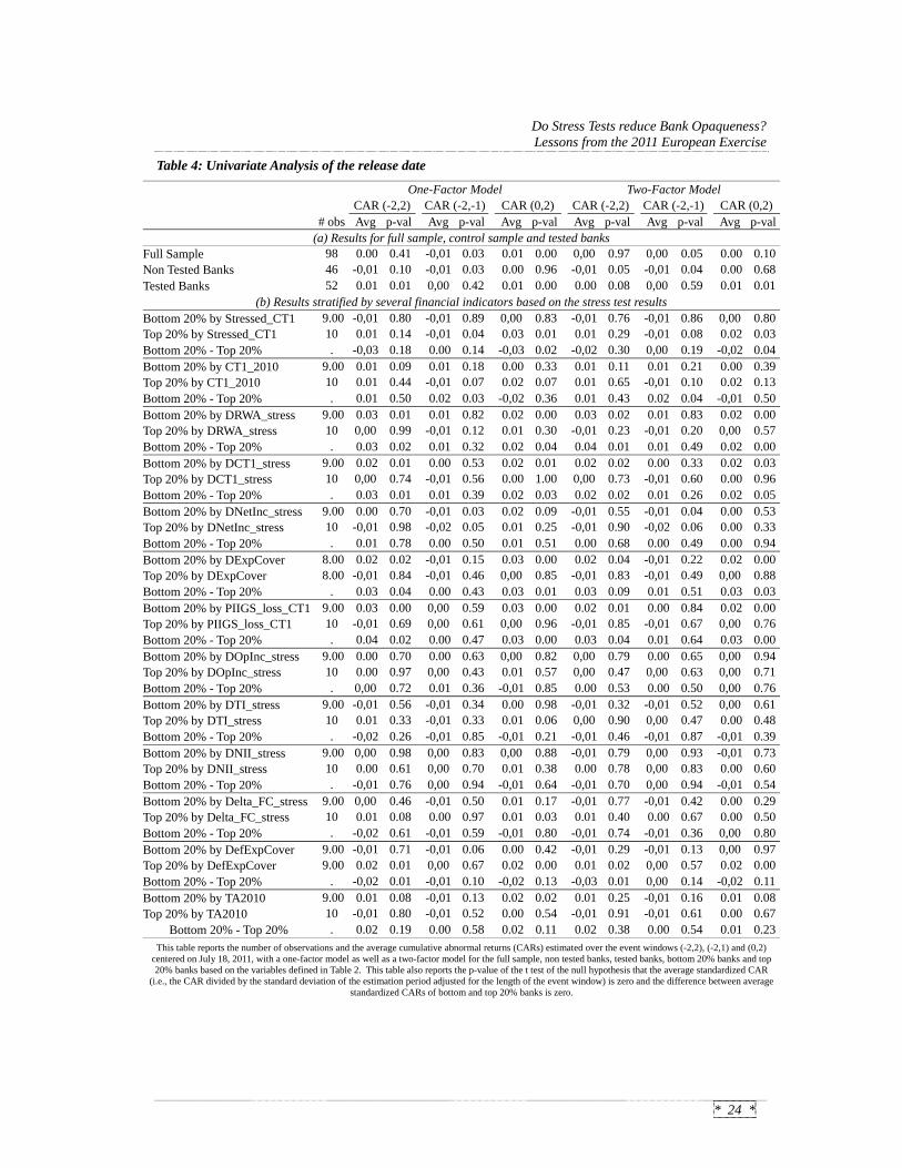
Table 4 provides detailed univariate tests on the release date. The layout is similar to Table
3, except that we do not rank banks only by Stressed_CT1, but instead use all the variables
in Table 2, since full details for all key indicators were known to the market at that time.
Tested banks show a positive reaction over the (-2, +2) window; this effect, however, is
statistically significant only in the post-event period (0,+2). The opposite is true for non-
tested banks: they experience weakly negative abnormal returns throughout the whole
event window, but price movements are significant only in the pre-event period.
Accordingly, tested banks are the only ones to experience a positive and statistically
significant reaction in the post-event period, most likely because of the results released by
EBA.
Do Stress Tests reduce Bank Opaqueness? Lessons from the 2011 European Exercise
* 23 *
This interpretation of the evidence is corroborated by the fact that, in the pre-event period,
almost no significant difference can be found between “top” and “bottom” tested banks
ranked according to several financial indicators35.
In the post-event period, instead, abnormal returns36 reward institutions which, under the
stressed scenario, manage to preserve a higher amount of Core Tier 1 capital
(Stressed_CT1), experience a lower drop in capital adequacy (DCT1_stress) and show a
less sharp increase in risk-weighted assets, write-downs and provisions (DRWA_stress,
DExpCov). Also, returns are better for banks less exposed to PIIGS sovereign debt
(PIIGS_loss_CT1).
Other determinants of net income (DOpInc_stress, DTI_stress, DNII_stress) prove less
significant; the same happens with the amount of eligible capital at end 2010 (CT1_2010)
and with variables which could indirectly capture some form of liquidity risk and model
risk (Delta_FC_stress, DefExpCover). It could well be that, while these relatively more
sophisticated indicators are not strong enough to explain CARs on a univariate basis, they
prove relevant when considered within a multivariate framework; further tests on this will
be produced in the next Section.
35 When one looks at the p-values for inter-quintile differences, only one out of 13 indicators falls below the
5% threshold (the Core Tier 1 ratio at end 2010). In this case, however, none of the two subgroups (Bottom and Top 20%) shows CARs that are different from zero at 5%. Accordingly, as mentioned in §5.2, in the next Section our multivariate analysis will focus on the post-event window only.
36 Results are robust to the market model used to generate abnormal returns (single-factor vs. two-factor model); further robustness checks across models will be produced in the multivariate analysis (§7).
Do Stress Tests reduce Bank Opaqueness? Lessons from the 2011 European Exercise
* 24 *
Table 4: Univariate Analysis of the release date
One-Factor Model Two-Factor Model CAR (-2,2) CAR (-2,-1) CAR (0,2) CAR (-2,2) CAR (-2,-1) CAR (0,2) # obs Avg p-val Avg p-val Avg p-val Avg p-val Avg p-val Avg p-val
(a) Results for full sample, control sample and tested banks Full Sample 98 0.00 0.41 -0,01 0.03 0.01 0.00 0,00 0.97 0,00 0.05 0.00 0.10Non Tested Banks 46 -0,01 0.10 -0,01 0.03 0.00 0.96 -0,01 0.05 -0,01 0.04 0.00 0.68Tested Banks 52 0.01 0.01 0,00 0.42 0.01 0.00 0.00 0.08 0,00 0.59 0.01 0.01
(b) Results stratified by several financial indicators based on the stress test results Bottom 20% by Stressed_CT1 9.00 -0,01 0.80 -0,01 0.89 0,00 0.83 -0,01 0.76 -0,01 0.86 0,00 0.80Top 20% by Stressed_CT1 10 0.01 0.14 -0,01 0.04 0.03 0.01 0.01 0.29 -0,01 0.08 0.02 0.03Bottom 20% - Top 20% . -0,03 0.18 0.00 0.14 -0,03 0.02 -0,02 0.30 0,00 0.19 -0,02 0.04Bottom 20% by CT1_2010 9.00 0.01 0.09 0.01 0.18 0.00 0.33 0.01 0.11 0.01 0.21 0.00 0.39Top 20% by CT1_2010 10 0.01 0.44 -0,01 0.07 0.02 0.07 0.01 0.65 -0,01 0.10 0.02 0.13Bottom 20% - Top 20% . 0.01 0.50 0.02 0.03 -0,02 0.36 0.01 0.43 0.02 0.04 -0,01 0.50Bottom 20% by DRWA_stress 9.00 0.03 0.01 0.01 0.82 0.02 0.00 0.03 0.02 0.01 0.83 0.02 0.00Top 20% by DRWA_stress 10 0,00 0.99 -0,01 0.12 0.01 0.30 -0,01 0.23 -0,01 0.20 0,00 0.57Bottom 20% - Top 20% . 0.03 0.02 0.01 0.32 0.02 0.04 0.04 0.01 0.01 0.49 0.02 0.00Bottom 20% by DCT1_stress 9.00 0.02 0.01 0.00 0.53 0.02 0.01 0.02 0.02 0.00 0.33 0.02 0.03Top 20% by DCT1_stress 10 0,00 0.74 -0,01 0.56 0.00 1.00 0,00 0.73 -0,01 0.60 0.00 0.96Bottom 20% - Top 20% . 0.03 0.01 0.01 0.39 0.02 0.03 0.02 0.02 0.01 0.26 0.02 0.05Bottom 20% by DNetInc_stress 9.00 0.00 0.70 -0,01 0.03 0.02 0.09 -0,01 0.55 -0,01 0.04 0.00 0.53Top 20% by DNetInc_stress 10 -0,01 0.98 -0,02 0.05 0.01 0.25 -0,01 0.90 -0,02 0.06 0.00 0.33Bottom 20% - Top 20% . 0.01 0.78 0.00 0.50 0.01 0.51 0.00 0.68 0.00 0.49 0.00 0.94Bottom 20% by DExpCover 8.00 0.02 0.02 -0,01 0.15 0.03 0.00 0.02 0.04 -0,01 0.22 0.02 0.00Top 20% by DExpCover 8.00 -0,01 0.84 -0,01 0.46 0,00 0.85 -0,01 0.83 -0,01 0.49 0,00 0.88Bottom 20% - Top 20% . 0.03 0.04 0.00 0.43 0.03 0.01 0.03 0.09 0.01 0.51 0.03 0.03Bottom 20% by PIIGS_loss_CT1 9.00 0.03 0.00 0,00 0.59 0.03 0.00 0.02 0.01 0.00 0.84 0.02 0.00Top 20% by PIIGS_loss_CT1 10 -0,01 0.69 0,00 0.61 0,00 0.96 -0,01 0.85 -0,01 0.67 0,00 0.76Bottom 20% - Top 20% . 0.04 0.02 0.00 0.47 0.03 0.00 0.03 0.04 0.01 0.64 0.03 0.00Bottom 20% by DOpInc_stress 9.00 0.00 0.70 0.00 0.63 0,00 0.82 0,00 0.79 0.00 0.65 0,00 0.94Top 20% by DOpInc_stress 10 0.00 0.97 0,00 0.43 0.01 0.57 0,00 0.47 0,00 0.63 0,00 0.71Bottom 20% - Top 20% . 0,00 0.72 0.01 0.36 -0,01 0.85 0.00 0.53 0.00 0.50 0,00 0.76Bottom 20% by DTI_stress 9.00 -0,01 0.56 -0,01 0.34 0.00 0.98 -0,01 0.32 -0,01 0.52 0,00 0.61Top 20% by DTI_stress 10 0.01 0.33 -0,01 0.33 0.01 0.06 0,00 0.90 0,00 0.47 0.00 0.48Bottom 20% - Top 20% . -0,02 0.26 -0,01 0.85 -0,01 0.21 -0,01 0.46 -0,01 0.87 -0,01 0.39Bottom 20% by DNII_stress 9.00 0,00 0.98 0,00 0.83 0,00 0.88 -0,01 0.79 0,00 0.93 -0,01 0.73Top 20% by DNII_stress 10 0.00 0.61 0,00 0.70 0.01 0.38 0.00 0.78 0,00 0.83 0.00 0.60Bottom 20% - Top 20% . -0,01 0.76 0,00 0.94 -0,01 0.64 -0,01 0.70 0,00 0.94 -0,01 0.54Bottom 20% by Delta_FC_stress 9.00 0,00 0.46 -0,01 0.50 0.01 0.17 -0,01 0.77 -0,01 0.42 0.00 0.29Top 20% by Delta_FC_stress 10 0.01 0.08 0.00 0.97 0.01 0.03 0.01 0.40 0.00 0.67 0.00 0.50Bottom 20% - Top 20% . -0,02 0.61 -0,01 0.59 -0,01 0.80 -0,01 0.74 -0,01 0.36 0,00 0.80Bottom 20% by DefExpCover 9.00 -0,01 0.71 -0,01 0.06 0.00 0.42 -0,01 0.29 -0,01 0.13 0,00 0.97Top 20% by DefExpCover 9.00 0.02 0.01 0,00 0.67 0.02 0.00 0.01 0.02 0,00 0.57 0.02 0.00Bottom 20% - Top 20% . -0,02 0.01 -0,01 0.10 -0,02 0.13 -0,03 0.01 0,00 0.14 -0,02 0.11Bottom 20% by TA2010 9.00 0.01 0.08 -0,01 0.13 0.02 0.02 0.01 0.25 -0,01 0.16 0.01 0.08Top 20% by TA2010 10 -0,01 0.80 -0,01 0.52 0.00 0.54 -0,01 0.91 -0,01 0.61 0.00 0.67
Bottom 20% - Top 20% . 0.02 0.19 0.00 0.58 0.02 0.11 0.02 0.38 0.00 0.54 0.01 0.23This table reports the number of observations and the average cumulative abnormal returns (CARs) estimated over the event windows (-2,2), (-2,1) and (0,2)
centered on July 18, 2011, with a one-factor model as well as a two-factor model for the full sample, non tested banks, tested banks, bottom 20% banks and top 20% banks based on the variables defined in Table 2. This table also reports the p-value of the t test of the null hypothesis that the average standardized CAR
(i.e., the CAR divided by the standard deviation of the estimation period adjusted for the length of the event window) is zero and the difference between average standardized CARs of bottom and top 20% banks is zero.

Do Stress Tests reduce Bank Opaqueness? Lessons from the 2011 European Exercise
* 25 *
6.2.2 Multivariate analysis
Our multivariate testing strategy is straightforward: we look at Figure 2 and take all
variables located on the final “leaves” of the tree starting from the stressed 2012 CT1 ratio.
These are: CT1_2010, DRWA_stress, DexpCover, DNII_stress and DTI_stress. By
focusing on variables which are not embedded into each other, we ensure that
multicollinearity issues are kept under control (see the pairwise correlations in Table 537).
We also test three other variables which, as shown in §5.3, are likely to add further insight
to the model: PIIGS_loss_CT1 (to express market concerns that the EBA approach on
sovereign losses may not have been conservative enough), Delta_FC_stress (impact on
funding costs of the stressed scenario, to proxy liquidity risk) and DefExpCov (coverage
ratio on defaulted exposures, which captures the “robustness” of the simulated losses to
worse-than-anticipated loss rates, and hence provides an indication, albeit very partial,
about each bank’s model risk).
Table 5: Pairwise correlations among regressors
CET1 ratio 2010
DRWAstress
DExp Cover
PIIGS loss
CET1
DNIMstress
DTI stress
Delta_FC stress
DefExpCover
CT1_ratio_2010 1 1% 21% 3% 19% -21% 8% 3%
DRWA_stress 1% 1 -28% -22% -28% 36% 10% -20%
DExpCover 21% -28% 1 54% 28% -48% -18% 30%
PIIGS_loss_CET1 3% -22% 54% 1 -4% -21% -19% 14%
DNII_stress 19% -28% 28% -4% 1 -21% 34% 5%
DTI_stress -21% 36% -48% -21% -21% 1 -16% -21%
Delta_FC_stress 8% 10% -18% -19% 34% -16% 1 0%
DefExpCover 3% -20% 30% 14% 5% -21% 0% 1
We start by testing all these potentially-relevant variables, and then move to a more
parsimonious model by gradually removing those which are not statistically significant.
The first and last step of this procedure are shown in Table 6; as a dependent variable we
use CARs on the (0, 2) window based on both a single-factor and a two-factor market
model (see columns I-II and III-IV, respectively).
37 Variance Inflaction Factors (VIFs) for the variables in Table 6 range from 1.1 to 2.3.

Do Stress Tests reduce Bank Opaqueness? Lessons from the 2011 European Exercise
* 26 *
Table 6: Cross-Sectional Determinants of the Market Reaction to the Stress Test Results
One-factor model
(local index) Two-factor model
(local and banks index)
(I) (II) (III) (IV)
Intercept -0,01 -0,03 0,00 -0,02 0,60 0,07 0,82 0,35
CT1_2010 0,51 0,57 0,45 0,48 0,00 0,00 0,01 0,00
DRWA_stress -0,02 -0,06 -0,07 0,31 0,03 0,00
DExpCover -1,01 -0,89 -0,91 -0,83
0,00 0,00 0,00 0,00
PIIGS_loss_CT1 -0,01 -0,01
0,23 0,54
DNII_stress 0,66 0,93
0,75 0,70
DTI_stress -7,17 -6,17
0,11 0,24
Delta_FC_stress [ x 103 ] -0,12 -0,11 -0,14 -0,12 0,02 0,05 0,03 0,04
DefExpCover 0,07 0,07 0,06 0,06 0,01 0,01 0,03 0,02
F-test 8,14 13,03 5,28 8,26
Prob > F 0,00 0,00 0,00 0,00
Adj R^2 0,58 0,58 0,44 0,46
# of obs 43 43 43 43
This table reports the results of weighted least squares (WLS) regressions of cumulative abnormal returns (CARs) over the (0, 2) event window, where 0 is the first trading day following the disclosure of the stress test results (i.e., July 18, 2011). The weight is the
inverse of the square root of the market model residual variance. The table shows the value of the coefficient estimates along with the p-value of their t-statistic (in italics). See Table 2 for
the definition of the explanatory variables.
The main results38 in the table are the following:
the models explain about half of the cross-sectional variance in CARs;
as shown in columns I and III, all tested variables have the expected sign, except
DNII_stress (which, however, is not statistically significant). Namely, a positive
market reaction appears to be associated with a higher amount of eligible capital at
end 2010, a decrease in the risk weights used to compute RWAs, lower credit
losses, lower involvement in PIIGS countries, a smaller drop in trading income
38 Results based on slightly wider or narrower event windows confirm most findings shown in Table 6,
although the significance of CET1_RATIO_2010 and Delta_FC_stress may sometimes decrease.

Do Stress Tests reduce Bank Opaqueness? Lessons from the 2011 European Exercise
* 27 *
(and a smaller increase in funding costs) under the stressed scenario, a higher
coverage of defaulted exposures;
the significance of DRWA_stress is weak and depends on the model used to
generate abnormal returns; this is not overly surprising, given that the change in
risk-weighted assets was only driven by changes in risk weights (the simulation
recipe prevented banks from de-leveraging);
besides net interest income, two other variables are consistently dropped when
moving from the complete model to the compact one; while DTI_stress may lack
relevance simply because trading income data was affected by the way each bank
had allocated securities between the trading and the banking book,
PIIGS_loss_CT1 (estimated losses on PIIGS exposures scaled by core Tier 1
capital) deserves further investigation, as data on sovereign exposures is thought to
have been one of the most noteworthy portion of the stress test results (and proved
relevant also in our univariate analysis); in §7.1 we control for a number of
alternative specifications;
variables proxying for liquidity risk and model risk prove significant across both
market models, suggesting that this type of information was appreciated by
investors (and more disclosure on those profiles would probably prove useful to the
market).
The above results have clear implications for the “stress hypothesis” stated in §4: variables
based on simulated data appear to be highly significant in driving the market reaction to
stress test results. Hence, the simulation exercise coordinated by EBA, while being openly
criticised by many analysts and commentators, seems to have provided investors with
relevant information.
The relevance of CT1_2010 provides support for the “zoom hypothesis”; however, it is
striking that the most important example of “zoomed” financial data included in the results
(the breakdown of sovereign exposures towards peripheral euro-zone countries) is
somewhat overriden by other indicators when tested on a multivariate basis. This will be
further investigated in the next Section.
Do Stress Tests reduce Bank Opaqueness? Lessons from the 2011 European Exercise
* 28 *
7 Further results and robustness checks
7.1 Sovereign risk and the zoom hypothesis39
As noted above, the lack of significance for PIIGS_loss_CET1 in Table 6 is somewhat
surprising. Details on sovereign debt holdings across countries and maturity bands were
considered highly informative by some equity analysts40, as they allowed to simulate the
impact of alternative stressed scenarios based on more severe assumptions. Indeed, EBA’s
chairman reportedly invited investors to “do the modelling themselves” based on such raw
data41. It is therefore important to verify whether such anecdotal evidence is confirmed by
abnormal price movements.
It could be that data on sovereign debt was in fact relevant, but PIIGS_loss_CT1 does not
capture the type of information actually used by investors . This could be due to a number
of reasons:
1. we are testing the wrong variable and a different specification would get different
results;
2. we are looking at data on sovereign debt holdings, but instead we should be
focusing on the unexpected component of such data, as only new information can
trigger price adjustments;
3. data on sovereign debt holdings partially duplicates information which is common
to other independent variables in Table 6, so one should look only at original
(orthogonal) information.
These possible explanations are now examined and tested in detail.
Different specifications - PIIGS_loss_CT1 might simply be a wrong way of capturing
sovereign risk, so different ratios could get better results. To address this concern we
experimented with a number of alternative variables. We first changed the numerator,
estimating possible losses on sovereign securities by multiplying the banks’ overall net
exposures (trading and banking book) to each country by the haircuts set by EBA for the
trading book (instead of applying a flat 25% loss rate to PIIGS countries and a 0% loss rate
the other ones). We then changed the denominator and used total assets as a scale variable,
39 This paragraph reports results for CARs generated through the two-factor market model. Results for the
single factor-based CARs are qualitative similar and available upon request. 40 See e.g. the reports by Goldman Sachs and Barclays quoted in (Onado 2011). 41 (Jenkins 2011).

Do Stress Tests reduce Bank Opaqueness? Lessons from the 2011 European Exercise
* 29 *
since using CT1 might duplicate information which already enters the model through
CT1_2010. Finally, we applied both changes jointly. Regression outcomes (available from
the authors) were similar to those shown in Table 6; hence our results appear robust across
alternative specifications for PIIGS-related losses42.
Unexpected information - Only new information reaching the market can cause abnormal
price adjustments, but sovereign debt holdings are not, per se, an unexpected piece of
news. Everybody expects Greek banks to hold a lot of Athens’ Treasury bonds, just like
OATs are most likely to be found in a French bank’s portfolio. What might matter more, in
our case, is whether an individual bank is holding an amount of PIIGS debt above or below
the average national level. To extract such unexpected component, we regress
PIIGS_loss_CT143 on a set of country dummies (see Table 7) and save the residuals
(measuring the gap between each institution and the country-specific mean) into a new
variable called Unexp_PLO (unexpected PIIGS-related losses).
Table 7: Estimation of unexpected losses on PIIGS exposures
Independent Variables:
AT BE CY DE DK ES FI FR GB GR HU IE IT MT NO PL PT SE
Coefficient 0,03 0,29 0,41 0,13 0,01 0,47 0,00 0,13 0,03 0,83 0,00 0,10 0,63 0,02 0,00 0,00 0,47 0,01
p-value 0,88 0,10 0,10 0,37 0,93 0,00 0,99 0,36 0,81 0,00 1,00 0,68 0,00 0,93 1,00 1,00 0,00 0,96
F-test 8,20
Prob > F 0,00
Adj R^2 0,73
# of obs 43
This table reports the results of an ordinary least square (OLS) regression of PIIGS_loss_CT1 (estimated loss on sovereign bonds issued by PIIGS over end-2010 Core Tier 1) over individual country dummies. The residuals of this regression are
referred to as 'Unexp_PLO' in Table 8.
We then take model (IV) in Table 6 and replace PIIGS_loss_CT1 with Unexp_PLO, to see
if this unexpected component has a stronger impact on abnormal returns. The result is
shown in Table 8, column (I): while the coefficient has the right sign (market prices drop
42 Holdings of Greek debt only (scaled by capital) are also found to be statistically irrelevant; although such
a ratio was found to significant in (Wolff 2011), the latter looks at stock returns between July and October 2011, hence it cannot be seen as (and is not meant to be) a study on stress test effects, but rather as an analysis of market reactions throughout the sovereign crisis.
43 As explained in §5.3, although the variable’s name refers to losses it also represents holdings of PIIGS debt, since the former are set equal to 25% of the latter.

Do Stress Tests reduce Bank Opaqueness? Lessons from the 2011 European Exercise
* 30 *
when exposure to PIIGS turns out to be higher than expected) it totally lacks statistical
significance44.
Table 8: Further results on sovereign exposures
(I) (II) (III)
Intercept -0,02 -0,01 -0,02 0,33 0,48 0,39
CT1_2010 0,47 0,44 0,47 0,00 0,01 0,00
DRWA_stress -0,07 -0,07 -0,07 0,00 0,00 0,00
DExpCover -0,85 -0,84 -0,85 0,00 0,00 0,00
Unexp_PLO -0,01
0,57
PLO_Orth -0,01
0,49
PLO_Orth_All -0,01 0,49
DeltaFC_stress [ x 103 ] -0,11 -0,12 -0,12 0,057 0,048 0,043
DefExpCover 0,07 0,06 0,06
0,02 0,02 0,02
F-test 6,81 6,87 6,87
Prob > F 0,00 0,00 0,00
Adj R^2 0,45 0,46 0,46
# of obs 43 43 43
This table reports the results of weighted least squares (WLS) regressions of cumulative abnormal returns (CARs) over the (0, 2) event window, where 0 is the first trading day following the disclosure of the stress test results (i.e., July 18, 2011). The weight is the
inverse of the square root of the market model residual variance. The table shows the value of the coefficient estimates along with the p-value of their t-statistcs. 'Unexp_PLO' is the
residual of the PIIGS_loss_CT1 variable regressed on individual country dummies. 'PLO_Orth_ChgExpCover' is the residual of the PIIGS_loss_CT1 variable regressed on the
ChgExpCover variable. 'PLO_Orth_All' is the residual of the PIIGS_loss_CT1 variable regressed on all the variables included in model (IV) reported on Table 6.
Original information – PIIGS_loss_CT1 is significantly correlated to other regressors in
our multivariate model, and namely to DExpCov (the variable measuring new write-downs
and provisions on credit exposures). The correlation between the two (see Table 5) is in
44 An alternative specification was also tested (not reported), where unexpected PIIGS losses/holdings were
proxied by PIIGS losses/holdings toward countries other than the one where the bank is legally headquartered; results were qualitatively similar.

Do Stress Tests reduce Bank Opaqueness? Lessons from the 2011 European Exercise
* 31 *
fact slightly higher than 50%. This is hardly surprising, as the rise in the expected loss rate
on sovereigns is one of the key factors causing provisions to increase under the stressed
scenario (as shown in Figure 2). Still, not all information in PIIGS_loss_CT1 is duplicated
by DExpCov (or by the other regressors in Table 6); actually, if the losses driving
DexpCov did not adequately mirror the banks’ individual exposures to sovereign risk, one
would expect the extra (i.e., original) information embedded in PIIGS_loss_CT1 to prove
highly relevant for abnormal returns.
To capture such “original information” we use the residuals of a regression of
PIIGS_loss_CT1 on DExpCov (see Table 9, column I) and call them PLO_Orth (PIIGS
losses made orthogonal). We then substitute PLO_Orth for PIIGS_loss_CT1 in Table 6 and
check whether PIIGS-related losses become more significant. The outcome (Table 8,
column II) looks quite weak: while the p-value slightly drops compared to equation (IV)
in Table 6 (49% vs. 54%), it still is too far from zero for PIIGS exposures to be relevant in
shaping the market’s reaction to stress test results. The same occurs (see variable
PLO_Orth_All in column III, Table 8) if, as a proxy for original information, one uses the
residuals obtained by regressing PIIGS_loss_CT1 (Table 9, column II) on all the
independent variables used in the last column of Table 6.
Overall, the results presented in this section confirm that data on sovereign exposures
appear of limited use when used jointly with other variables taken from EBA’s “stressed”
scenario. This means that, even though political constraints prevented the European
supervisor from making extreme assumptions (like the default of one or more euro-zone
countries), the individual weaknesses and vulnerabilities highlighted by the stress test were
still considered credible and reasonably accurate by market participants. The alternative
explanation (that detailed data on sovereign exposures have been snubbed by investors
simply because their quality/granularity was deemed too poor45) would not explain why
such data prove significant when considered on a stand-alone basis.
45 Data quality issues were, in fact, present. As noted by (Das 2011), for example, one British bank only
disclosed the European credit exposures in its UK operation, omitting exposures held through other entities below the 5% EBA disclosure threshold. One Italian bank did not separately disclose Eastern European exposures, as they were held via their subsidiary in Austria

Do Stress Tests reduce Bank Opaqueness? Lessons from the 2011 European Exercise
* 32 *
Table 9: Orthogonalisation of Sovereign Exposures (PIIGS_loss_CT1)
(I) (II)
Intercept 0,04 0,40 0,63 0,22
CT1_2010 -5,18 0,04
DeltaFC_stress [ x 103 ] 0,38 0,73
DefExpCover 0,10 0,84
ChgExpCover 10,82 11,81 0,00 0,00
DRWA_stress -0,15
0,72
F-test 16,46 4,31
Prob > F 0,00 0,00
Adj R^2 0,27 0,28
# of obs 43 43
Model I is the ordinary least square (OLS) regressions of PIIGS_loss_CT1 (the estimated loss on sovereign bonds issued by PIIGS over 2010 Core Tier 1) on the change in coverage ratio for credit exposures from 2010 to stressed 2012 (in model (I); its residuals are referred
to as 'PLO_Orth' in Table 8). Model II is the OLS regression of PIIGS_loss_CT1 on the explanatory variables shown in Table 6, column (IV); its residuals are referred to as
'PLO_Orth_All' in Table 8). The table shows the value of the coefficient estimates along with the p-value of the t-statistic (in italics)
7.2 Eligible capital and “small” banks
One of the most significant regressors in Table 6 is CT1_ratio_2010, the Core Tier 1 ratio
at end 2010 (adjusted by all mitigating measures that were irrevocably committed by end
April 2011). As mentioned in §6.2.2, one could wonder why a variable based on the 2010
financial statement had not already been discounted by market prices. Our explanation is
that CT1_ratio_2010 may indeed convey new (“zoomed”) information as it tells investors
about the actual capital items and deductions that EBA and national supervisors deemed
appropriate for each bank. If this were the case, then CT1_ratio_2010 is likely to be
especially relevant for smaller banks, as equity analysts and rating agencies can be
expected to have already produced accurate estimates of “eligible capital” for larger
institutions.
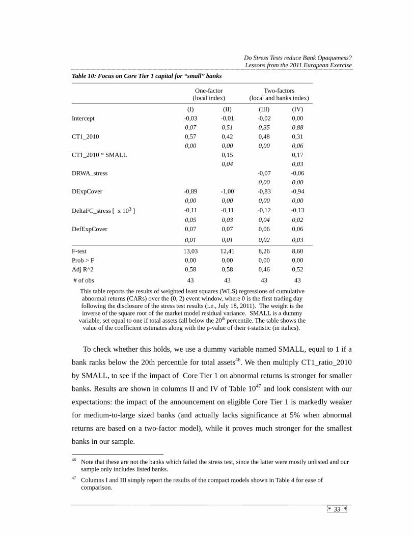
Do Stress Tests reduce Bank Opaqueness? Lessons from the 2011 European Exercise
* 33 *
Table 10: Focus on Core Tier 1 capital for “small” banks
One-factor
(local index) Two-factors
(local and banks index)
(I) (II) (III) (IV)
Intercept -0,03 -0,01 -0,02 0,00 0,07 0,51 0,35 0,88
CT1_2010 0,57 0,42 0,48 0,31 0,00 0,00 0,00 0,06
CT1_2010 * SMALL 0,15 0,17 0,04 0,03
DRWA_stress -0,07 -0,06 0,00 0,00
DExpCover -0,89 -1,00 -0,83 -0,94 0,00 0,00 0,00 0,00
DeltaFC_stress [ x 103 ] -0,11 -0,11 -0,12 -0,13 0,05 0,03 0,04 0,02
DefExpCover 0,07 0,07 0,06 0,06
0,01 0,01 0,02 0,03
F-test 13,03 12,41 8,26 8,60
Prob > F 0,00 0,00 0,00 0,00
Adj R^2 0,58 0,58 0,46 0,52
# of obs 43 43 43 43
This table reports the results of weighted least squares (WLS) regressions of cumulative abnormal returns (CARs) over the (0, 2) event window, where 0 is the first trading day following the disclosure of the stress test results (i.e., July 18, 2011). The weight is the inverse of the square root of the market model residual variance. SMALL is a dummy
variable, set equal to one if total assets fall below the 20th percentile. The table shows the value of the coefficient estimates along with the p-value of their t-statistic (in italics).
To check whether this holds, we use a dummy variable named SMALL, equal to 1 if a
bank ranks below the 20th percentile for total assets46. We then multiply CT1_ratio_2010
by SMALL, to see if the impact of Core Tier 1 on abnormal returns is stronger for smaller
banks. Results are shown in columns II and IV of Table 1047 and look consistent with our
expectations: the impact of the announcement on eligible Core Tier 1 is markedly weaker
for medium-to-large sized banks (and actually lacks significance at 5% when abnormal
returns are based on a two-factor model), while it proves much stronger for the smallest
banks in our sample.
46 Note that these are not the banks which failed the stress test, since the latter were mostly unlisted and our
sample only includes listed banks. 47 Columns I and III simply report the results of the compact models shown in Table 4 for ease of
comparison.
Do Stress Tests reduce Bank Opaqueness? Lessons from the 2011 European Exercise
* 34 *
8 Final remarks
Stress tests are complex exercises involving scenario design, extensive data gathering,
close interaction between banks and supervisors, repeated assessment of the internal
models and assumptions used by the former, careful calibration and timely disclosure of
the final results.
The current debate on their ability to reduce bank opaqueness is often based on anecdotal
evidence or event windows biased by unrelated events.
In this paper we examine the 2011 European stress test exercise, which provided investors
with an unprecedented amount of data on 90 large European banks, to assess whether and
how it affected stock prices. We find evidence of significant market reactions both on
various pre-release announcement dates and upon the release of the test’s detailed (i.e.,
bank-by-bank) results.
The initial announcement of the 2011 stress test exercise (and the decision to publicly
disclose its results) was accompanied by a rise in the stock prices of tested banks, while
untested banks share prices were unaffected. This is consistent with the hypothesis that the
market welcomes the stress test exercise as a way to trim bank opacity costs. We observe a
price drop around the second announcement, when supervisors made reference to possible
“remedial measures” (i.e., capital increases), possibly due to dilution fears. We also find a
positive market reaction (especially for the more capitalized banks) around the
announcement of a stricter definition of capital to be used in the stress test exercise.
The irrelevance hypothesis is further weakened by the market reaction to the disclosure of
detailed stress test results. Tested banks show a significant price rise, unparalleled by non-
tested ones, and their abnormal returns depend on a number of bank-specific factors. While
it cannot be ruled out that CARs be driven by detailed information on current financial data
(the “zoom hypothesis”), ratios expressing the banks’ vulnerability/resilience to a downturn
scenario clearly play a major role. This supports the “stress hypothesis” and indicates that
stress tests, although politically constrained (as well as affected by model risk and data
quality issues), provide investors with relevant information and can be used as an effective
tool to address bank opacity.
Do Stress Tests reduce Bank Opaqueness? Lessons from the 2011 European Exercise
* 35 *
9 Appendices
Appendix 1 - The main assumptions in the EBA 2011 stress tests
The stress test exercise was based on financial data as of December 31, 2010 and covered
a period of two simulated years (2011 and 2012). Two scenarios were tested: baseline and
adverse. Under the baseline scenario a strengthening of macroeconomic recovery was
assumed, with GDP growth of 1.7% and 2% in the EU. Under the adverse scenario, GDP
would shrink by 0.4% in 2011, then stay flat in 2012; meanwhile, equity prices would drop
by 15%, short-term risk-free rates would increase by 1.40% and long-term ones by 1.25%.
Credit spreads for sovereign debts in Europe would also pick-up, with different increases
for individual countries. The USD would devaluate by 11%.
Banks had to translate these assumptions into their balance sheets based on a “zero growth
and constant mix” approach, whereby maturing assets and liabilities were to be replaced by
equivalent ones (e.g., the proportion of retail and wholesale liabilities had to be kept
constant). The main criteria to be followed by banks to generate simulated results are
summarized below.
Defaulted loans had to be estimated by multiplying outstanding balances by expected
default rates (accounting for the effects of the adverse scenario where appropriate). The
increase in non-performing loans would negatively affect interest receivable.
Migrations of risk-weighted assets across different rating/PD buckets had to be simulated
by the banks subject to a subsequent review by EBA and national supervisors. IRB banks48
also had to estimate the deterioration in downturn LGDs following from adverse
macroeconomic conditions, in order to assess the overall increase in expected losses and
regulatory RWAs. RWAs at end 2010 would in any case act as a floor to the banks’
projections.
As regards expected losses in the adverse scenario, EBA had asked banks to apply a 40%
LGD and a set of predetermined PDs to exposures towards banks and sovereigns located in
different countries (e.g., exposures to Greek counterparts would be subject to a 36% PD).
Full provisions against such expected losses had to be charged onto the P&L account.
48 In the Basel 2 jargon, IRB banks are those allowed to use internal rating models to compute minimum
regulatory capital.

Do Stress Tests reduce Bank Opaqueness? Lessons from the 2011 European Exercise
* 36 *
Securities in the trading book (as well as equity holdings in the “available for sale”
portfolio) had to be marked to market based on the parameters underlying the
macroeconomic scenario. RWAs on market risk had to be increased to account for the new
Basel rules (“stressed VaR”, “incremental risk charge”); banks unable to provide internal
estimates were asked to apply a 250% scaling factor to 2010 data.
Capital was expected to change due to retained profits, losses and maturing Tier2 issues.
Any extraordinary measure (including government support) agreed upon and committed by
April 30, 2011 could be factored in, but had to be highlighted separately. Retained profits
were estimated based on the median payout ratio for the last three years.
The shift in market rates had to be translated into the banks’ lending and funding rate
based on a conservative approach. The increase in risk-free rates could be passed on only
to variable-rate loans and rolled-over ones; only 50% of the rise in the bank’s own credit
spread (set equal to the 2-year sovereign spread) could translate into higher lending rates.
As regards interest expenses, the banks had to account for an immediate 100% rise of
wholesale funding costs, a partial increase in the cost of retail deposits (in line with past
records, but also accounting for stronger competition in that market) and a drop in the
value of sovereign assets used as collateral in funding transactions.
Commissions, dividend income and administrative costs had to be kept in line with 2010
levels. Trading income had to be estimated by taking the average amount for the last five
years and applying the loss rates implied by the macroeconomic scenario (e.g., a 15%
stock-market drop, haircuts due to the increase in interest rates and credit spreads, etc.).
Impairments on defaulted loans had to be simulated based on the banks’ forecasts for loss
rates (“LGD”). This included new defaulted exposures, as well as a re-assessment of the
loss rates on previously defaulted positions that had not yet been written-off.

Do Stress Tests reduce Bank Opaqueness? Lessons from the 2011 European Exercise
* 37 *
10 Bibliography
Beltratti, Andrea. 2011. Do stress tests carry useful information? Evidence from Europe. mimeo, Bocconi University, October.
Blundell-Wignall, A., and P. Slovik. 2010. The EU stress test and sovereign debt exposures. OECD.
Boehmer, E., J.P. Broussard, and J.P. Kallunki. 2002. Using SAS in financial research. Sas Inst.
Bryant, Chris. 2011. “German banks hit at data plan.” Financial Times Europe, July 12.
Campbell, J.Y., A.W. Lo, and A.C. MacKinlay. 1997. The econometrics of financial markets. Vol. 1. princeton University press Princeton, NJ.
Cardinali, Andrew, and Jakob Nordmark. 2011. How informative are Bank Stress Tests? Bank Opacity in the European Union. Lund University.
Committee of European Banking Supervisors. 2010. Aggregate outcome of the 2010 EU wide stress test exercise coordinated by CEBS in cooperation with the ECB. Committee of European Banking Supervisors.
Das, Satyajit. 2011. The EBA Stress Tests - Not the Real Thing. Eurointelligence. July 26. http://www.eurointelligence.com/eurointelligence-news/home/singleview/article/the-eba-stress-tests-not-the-real-thing.html.
Dennis, Neil. 2011. “Gains for Commerzbank and Unicredit as banks perk up.” Financial Times Europe, July 22.
European Banking Authority. 2011a. EU-wide Stress Test: Methodological Note. European Banking Authority.
---. 2011b. EU-wide Stress Test: Methodological Note, Additional Guidance. European Banking Authority.
Federal Reserve. 2009a. The Supervisory Capital Assessment Program: Design and Implementation. Federal Reserve, Washington DC.
---. 2009b. The Supervisory Capital Assessment Program:Overview of Results. Federal Reserve, Washington DC.
Financial Times. 2011. “Recapitalisation cal catches Europe off guard.” Financial Times Europe, August 29.
Flannery, Mark .J., Simon H. Kwan, and M. Nimalendran. 2010. “The 2007–09 Financial Crisis and Bank Opaqueness.” Working Paper Series, Federal Reserve Bank of San Francisco.
Flannery, Mark J., Simon H. Kwan, and M. Nimalendran. 2004. “Market evidence on the opaqueness of banking firms’ assets.” Journal of Financial Economics 71 (3): 419-460. doi:10.1016/S0304-405X(03)00185-5.

Do Stress Tests reduce Bank Opaqueness? Lessons from the 2011 European Exercise
* 38 *
Haggard, K.S., and J.S. Howe. 2007. Are banks opaque. unpublished working paper, University of.
Hirtle, Beverly, Til Schuermann, and Kevin J. Stiroh. 2009. “Macroprudential Supervision of Financial Institutions: Lessons from the SCAP.” SSRN eLibrary (November 1). http://papers.ssrn.com/sol3/papers.cfm?abstract_id=1515800.
Iannotta, G. 2006. “Testing for opaqueness in the European banking industry: evidence from bond credit ratings.” Journal of Financial Services Research 30 (3): 287–309.
Jenkins, Patrick. 2011. “Quality of stress test disclosures a mixed bag.” Financial Times Europe, July 18.
Jordan, J. 2000. “The Market Reaction to the Disclosure of Supervisory Actions: Implications for Bank Transparency.” Journal of Financial Intermediation 9 (July): 298-319. doi:10.1006/jfin.2000.0292.
MacKinlay, A.C. 1997. “Event studies in economics and finance.” Journal of economic literature 35 (1): 13–39.
Morgan, D.P. 2002. “Rating banks: Risk and uncertainty in an opaque industry.” American Economic Review: 874–888.
Onado, Marco. 2011. European stress tests: Good or bad news? www.voxeu.com. August 16. http://www.voxeu.com/index.php?q=node/6878.
Peristiani, S., D.P. Morgan, and V. Savino. 2010. “The Information Value of the Stress Test and Bank Opacity.” FRB of New York Staff Report No 460 (July).
Quagliariello, Mario. 2009. Stress-testing the banking system: methodologies and applications. Cambridge University Press, October 15.
Spiegel, Peter, and Quentin Peel. 2011. “Deal agreed on Greece bailout.” Financial Times Europe, July 22.
The Economist. Europe’s banks: Ignoring the obvious | The Economist. zotero://attachment/123/.
Thompson, R. 1995. “Empirical methods of event studies in corporate finance.” Handbooks in Operations Research and Management Science 9: 963–992.
Weston, J.F., M.L. Mitchell, and J.H. Mulherin. 2004. Takeovers, Restructuring & Corporate Governance International Edition, 4th Edition. 4th ed. Upper Saddle River (NJ): Prentice Hall, ISBN 0-13-122553-7.
Wolff, Guntram B. 2011. “Is recent bank stress really driven by the sovereign debt crisis?” Bruegel Policy Contribution (12).