January 14, 2000

Building Community Institutions to Manage Local Resources:

An Empirical Investigation

Eric V. Edmonds∗∗∗∗

Department of Economics

Dartmouth College

Abstract

The lack of well-defined property rights causes the Tragedy of the Commons. Transferring common property to local communities for management has become the primary prescription for eliminating the incentives driving the Tragedy. Building community institutions to manage local resources is a critical component of the recent emphasis on “sustainable development.” Despite substantial theoretical consideration of indigenous community resource management, there is little empirical evidence on the efficacy of government initiated, community institutions. This paper uses variation in the timing of implementation of a massive institutional reform in Nepal to identify the impact of newly created community user groups on household forest use. Transferring forest property to local user groups substantially reduces household resource extraction.

∗ I received financial support on this paper from the National Science Foundation, the John D. and Catherine T. MacArthur Foundation, and the Andrew W. Mellon Foundation. I have benefited from the insights and assistance of Marianne Bertrand, Kristin Butcher, Anne Case, Angus Deaton, Karla Hoff, Bo Honore, Keshav Karmacharya, Doug Miller, Jonathan Morduch, Nina Pavcnik, Chris Paxson, Giovanna Prennushi, Yam Raya, K.B. Shrestha, Rajendra Shrestha, and Sanjay Verma. I am grateful for the many helpful comments of seminar participants at Boston College, Cornell University, Dartmouth College, Michigan State University, North Carolina State University, Princeton University, William and Mary, and Williams College. Correspondence to: Eric Edmonds, Department of Economics, 6106 Rockefeller Center, Hanover, NH 03755. Eric.Edmonds@dartmouth.edu.

2

I. Introduction

The “Tragedy of the Commons” occurs, because open access to a scarce resource prevents rents

from accruing to that resource. Thus, the resource is overexploited (Gordon 1954). Traditionally,

nationalization and privatization have been the two main policy solutions prescribed to prevent the

tragedy of the commons. In many cases, the success of nationalization has been hampered by imperfect

incentives and prohibitively large information and monitoring costs. Though many economists have been

advocating privatization of the commons for decades (Coase 1960, Demsetz 1967), concerns about

fairness and widespread anecdotes of abuse have contributed to substantial political resistance to

privatization (Dasgupta 1993). Spurred by extensive research on indigenous community institutions,

community management of common property has risen as a popular alternative for the commons (Ostrom

1990, Baland and Platteau 1996). Recent environmental conferences such as the 1992 Earth Summit and

the United Nations Conference on Environment and Development have taken the position that

“sustainable development” requires community management of resources (Leach, et al 1999). This paper

considers the impact of government initiated community institutions to manage local resources on local

resource extraction.

Government initiated community institutions might not impact local resources in the same way as

indigenous institutions. A large theoretical literature shows that communities, under certain restrictive

conditions, can develop mechanisms limiting extraction from common property (see Sethi and

Somanathan 1996 for a recent discussion), but these models do not generalize to institutions imposed on

communities. Large-scale implementation of community-based management requires that communities

manage the resource independent of the implementing agent. Hence, it is unclear whether these

unsolicited institutions will continue to function without external supervision. The small theoretical

literature on government initiated community management focuses entirely on co-management of local

resources by communities and governments (Baland and Platteau 1996, Ligan and Narian 1999), and the

empirical literature on government initiated community institutions is limited to case studies of small,

nonrandom projects operating with extensive external assistance and oversight. This study examines the

3

impact of government initiated community institutions on local resource extraction using a massive

program in Nepal that transferred all of Nepal’s accessible forestland to community groups of forest

users.1 We find that government initiated community institutions to manage local resource are associated

with a statistically significant reduction in resource extraction.

We base this study on a household survey collected two years after the passage of the act handing

over forestland to local communities. Transferring every accessible forest over to local communities is

time consuming and costly. At the time of the survey, significant portions of the country have not

received user groups yet. We use variation in the timing of the implementation of user groups to identify

the effects of the program. In our analysis, we compare areas that have received forest groups to areas

that have not. This raises econometric issues associated with unobserved differences between areas with

and without forest groups. To overcome this evaluation problem, we use institutional information and

administrative records to control for the nonrandom assignment of forest groups. We show that the

creation of user groups is associated with a more than ten percent reduction in resource extraction and this

result is robust to various identification strategies.

The next section outlines the household’s resource extraction problem. The operation of user

groups is explained and incorporated into the household model. Section III builds a model of user group

formation and incorporates the model into a discussion of the program evaluation problem in this study.

Section IV applies the insights of section III to data from eastern Nepal. Section V concludes.

II. Institutions in the Resource Extraction Problem

Throughout this paper, we focus on the household’s fuelwood collection problem as our measure

of resource extraction. The collection of wood for fuel is one of the two main causes of deforestation in

Nepal (agricultural conversion of forest land is the other: Soussan, et al 1995). While forest user groups

1 Community (or social) forestry is the moniker applied to the government creation of community institutions to manage local forests. Smaller community forestry programs are currently being implemented throughout the world including countries such as India, Thailand, Indonesia, the Philippines, Kenya, Nigeria, Ethiopia, Ghana, South Africa, Peru, and Brazil.

4

generally have well defined boundaries that can limit agricultural conversion of forest user group land, the

impact of forest user groups on household collection activities is unclear. To examine, the impact of

forest groups on forest use, we adapt the basic farm household model explored in Singh, Squire, and

Strauss (1986) to the problem the household solves when it decides how much firewood to collect.2

In the simplest household model, households have preferences over firewood y and some

other good l (l may be a vector in a more elaborate framework). These preferences have a utility

representation U that may depend on household characteristics X. G() summarizes the tradeoff

between firewood and some other good x. G() reflects resource and technology constraints (l

might be leisure so that –l is labor, and G() is a production function). Firewood may be

purchased at relative price p.3 A household produces firewood until the value of the marginal

product of –l in the production of firewood is equal to its opportunity cost. The household

purchases any additional firewood that it needs to consume its most preferred, attainable bundle

of firewood and good l. Figure 1a is the simple graphical representation of this model outlined in

Benjamin (1992).

2 Significantly more complicated frameworks have been applied to the household’s wood for fuel collection problem (Amacher, et al 1996; Heltberg, et al 2000). While these models unquestionably are more accurate depictions of the household’s decision-making problem, they do not bring any additional insight to the evaluation problem presented in this paper. 3 In a non-separable framework, the relative price is actually the (endogenous) opportunity cost of the labor used in firewood collection. This is the substantive difference between the treatment here and the treatment in the two papers mentioned in the previous footnote. This treatment does not change the conclusions we draw below in part B of this section.

5

Figure 1: Separable Farm Household Model (Benjamin 1992)

Firewood

-l

Collected Firewood

Total Firewood

G(l;X)

U(-l,y;X)

Slope is p

A. Forestry Institutions in Nepal

The staff of His Majesty’s Government’s Department of Forests creates forest user groups in Nepal.

Prior to 1993, all forests in Nepal were the property of His Majesty’s Government, and the Department of

Forests existed to protect and maintain Nepal’s forests.4 With the transfer of all accessible national

forests to local users in the Forest Act of 1993, the work of the Department of Forests turned to creating

forest groups.

The Department of Forests field staff is given a basic operational plan and a constitution that the field

staff adapts to each forest group. The forest user group constitution details how user group committees

are constructed, how disputes are resolved, how land territory and borders are defined, and who are

members of the group. User group committees meet periodically to handle all management decisions

regarding the forest. The operational plan describes the activities permissible on user group land.

Typically, the operational plan prohibits grazing on forestland. Most plans specify what products can and

cannot be removed from the forest, who can remove them, and when products can be removed. Prices are

set for products that can be removed. These prices are usually in the form of per unit taxes on the

4 In 1957, all forests over 1.25 hectares in the mountain and hill areas of Nepal and all forests over 3.25 in the flat Terai area of Nepal were nationalized.

6

collecting household.5 Prices for user group members and nonmembers are specified and typically differ

(nonmembers are charged more for using the forest). In practice, nonmembers are often excluded from

using the user group land altogether. Also, most operational plans specify an access fee in addition to or

as an alternative to the extraction tax. These fees gain the household entrance into the forest. Many

operational plans frame these access fees as membership fees that must be paid annually or paid in

advance to join the forest user group. Thus, the mechanisms open to forest groups to effect forest use are

a ration, exclusion (a ration of zero), an access fee, or an output tax.

While the constitution and the operational plan define how a user group is supposed to operate, a

group’s actual operation can vary substantially from these guidelines. The field staff has been

overextended with the formation process; the staff has few opportunities to oversee group operation

(Gibbon 1996). Usually, the field staff helps the forest group take control of the land and provide

assistance in fencing the forest and hiring a forest guard (Chhetri and Nurse 1992). When the field staff is

available for additional support, the staff assists with forest nurseries or income-generating activities

(Chhetri and Pondey 1992). Thus, user groups are free to implement their constitutions and operational

plans as they choose.

B. Forest Institutions in the Farm Household Model

The motivation behind community forestry is to internalize the externality associated with extraction

into the household’s fuelwood collection problem (or equivalently to make the household pay rent to the

forestland). Thus, absent any supply effects, households reduce their use of the forest. All of the

different mechanisms open to forest groups (assuming that firewood is a good) reduce firewood

collection.6 Unfortunately, it is not possible to identify which of the separate mechanisms are at work.

5 No forest user groups in the area of our sample of households reported selling harvested firewood directly to market (author’s calculation from the Nepali-United Kingdom Community Forestry Database 1997). 6 Reduced firewood collection should allow the forest to regenerate. Thus, the long-term effect of forest groups could be greater firewood collection, because the supply effects might dominate the effects of the taxes imposed. However, the time to regenerate a forest in the Arun Valley is substantially longer than the short time forest groups have been operating in the Arun Valley (Shrestha 1989).

7

Consider an access fee. There are several different ways the access fee could affect household

behavior. Assume the access fee is assessed in firewood units. First, in the simplest (separable) version of

the model in figure 1, the access fee shifts G(), but does not change the shape of G(). Since the price line

does not change, then the slope of G() at the point where the household stops collecting and starts

purchasing does not change. This is illustrated in figure 1B.

Figure 1B: Downward Shift in G

Firewood

-l

Collected Firewood

Total Firewood

G(l;X)

U(-l,y;X)

Shift from Access Fee

Figure 1C: Change in Shape of G

Firewood

-l

Collected Firewood

Total Firewood

U(-l,y;X)

Old Forest w/ Access Fee

Substitute Forest

A second possibility is that if the household chooses to collect from an alternative forest (without an

access fee) rather than pay the access fee, the shape of G() changes to reflect the production technology in

the alternative forest. Figure 1C is an example of this. Thus, a precise characterization of the effect of an

access fee is very difficult.

A ration or exclusion is just as ambiguous. One potential effect is that the household's collection

is limited to the ration. In this case, if we possessed more price data (only 70 households report a purchase

price of firewood), we could recover the kink in household firewood demand from the ration. However, if

there exist other forests that have not been transferred to user group control, households may just collect

from these alternative forests. In this way, collection becomes more costly, and the ration is not visible in

the data. Another possibility is that the ration makes firewood more abundant (and less costly to collect)

to households that have access to the user group forest. When certain households are excluded and others

8

are not, fuelwood collection could become cheaper for included households and more costly to excluded

households.

Thus, identifying different mechanisms used by forest user groups to lower fuelwood extraction is

not feasible with the data available. In what follows, we limit discussion to whether or not forest user

groups reduce household fuelwood collection and leave the question of how forest user groups do this

unanswered.

III. The Evaluation Problem

The aim of this paper is to understand the impact of transferring forests to local communities on forest

use. We address this question by comparing areas with and without forest user groups. This section

spells out the evaluation problem this type of comparison occasions. We begin with background

information on the area studied, build a model of forest group formation in the study area, and then

incorporate this model into the program evaluation problem.

A. Background Information

In this paper, we use data from the Arun Valley of Nepal. The Arun Valley constitutes three districts

in Eastern Nepal, and the household survey used in this paper is based on a random sample of households

from these three districts. The World Bank and the Central Bureau of Statistics in Kathmandu jointly

conducted the survey (the Arun Valley Living Standards Study, “ALSS”). 1200 households in 100

communities were sampled during one Nepali calendar year that spanned 1995 and 1996 of the Gregorian

calendar.7 This is two years after the passage of the Forest Act, transferring all forested land to local

users.

7 Each district in Nepal is divided into VDCs (Village Development Committees). The VDC is the main local government agent, and there are more than thirty VDCs per district typically. Each VDC is divided into eight wards usually. The ward is the smallest level of administration in Nepal, and it is the definition of community used throughout this paper.

9

The Arun Valley refers to the watershed surrounding the Arun River. Shrestha (1989) describes

the economy and the environment of the Arun Valley. Almost the entire valley is accessible only by

footpath and the economy is largely subsistence. Over 70% of the adult population never received any

schooling. The terrain is mountainous and varied, characterized by few flat areas, and ranging in

elevation from sea level near the river’s base to 8,470 meters at the top of Mt. Makalu-Barun.

Forest Policy in all three districts is coordinated by one organization, the Nepali-United Kingdom

Community Forestry Project (NUKCFP). The NUKCFP database (1997) is a census of all forest user

groups in the Arun Valley. This database is matched to the Arun Valley Living Standards Survey in order

to identify the location and formation dates of forest groups. The NUKCFP funds and trains all of the

foresters in the three districts of the Arun Valley, and it provides the field staff with the basic operational

plans and constitutions used in the creation of forest groups. The forest staff in each district consists of a

District Forest Officer and then his field staff (forest rangers, forest guards) that creates forest groups.

The field staff operates out of range posts spread throughout the district.

B. The Formation of Forest Groups

The user group formation process takes place in four general steps.8 First, a forester selects a

forest to hand over to a user group. Second, the forester decides who are the users of this forest. The user

identification process generates controversy since the field staff depends on local leaders to name forest

users (Gurung, et al 1996; Kafle 1997). Third, the forester organizes the users and holds a meeting of all

user group members. In this meeting the field staff helps group members create a group constitution, fill

out an operational plan, and elect committee members in charge of the daily operations of the group.

Fourth, the forester submits the operational plan and constitution to the Department of Forests in

Kathmandu. Once these documents are approved, the forest user group (FUG) is officially formed.

8 These four steps are my summary of the formation process defined in the Operational Guideline for Community Forestry Development Programme 2051. These steps can be interpreted as broad categories for the rules and procedures outlined in the Community Forestry Manual 1995. They correspond to the formation process that I observed during my fieldwork.

10

The Forest Act does not stipulate how foresters decide what areas get user groups first, because

all accessible forests are to be turned over to user groups immediately (Community Forestry Manual

1995). The implementation process is time consuming, and thus implementation has occurred more

gradually than envisioned in the law. By the time of the household survey used in this paper, less than ten

percent of the forestland in Nepal has been transferred to user groups (see Edmonds 1999 for greater

detail on the implementation of community forestry throughout Nepal). This section outlines a simple

model of how the field staff forms forest groups.

Consider a forester faced with the decision of where to form a group next. The forester gets some

payoff from forming a forest group. The forester’s payoff depends on the effort the forester must put into

forming the group, e, and how accessible the forest area is to the forester, a. Let the forester’s payoff be

represented by the function v=V(e,a). Assume V is increasing in a and decreasing in e. The forester

knows that all areas must receive forest groups, but discounts the future so he chooses to form groups in

areas with the highest payoff (least effort, most accessible) first.

The forester’s payoff does not depend on the quality of the forest area being transferred.

Relaxing this assumption does not change the interpretation of the second part of our identification

strategy (section IV, part B), and it is likely to be a realistic assumption. All accessible forest area will be

transferred to forest groups eventually. Thus, the payoff of transferring more (or less) degraded

forestland first, is purely in the benefit to the forest of being transferred today versus in a few years.

Shrestha (1989) notes the forests in the Arun Valley face a long regenerative cycle. Consequently, even if

the forester cares about the outcome on the forest area, the extra benefit to the forest from transferring one

type of forest first is likely to be minimal, especially when compared with the cost and inconvenience of

going to an unfamiliar area several days trek from the range post.

Effort e captures how difficult the forester expects it to be to form a group in an area. It is unclear

whether or not this effort varies from community to community. The forester fills out the operational

plan and constitution for the community. Hence, this step does not require the active cooperation of

community members. Given the lack of monitoring of group activities, there is no reason why a

11

community would object or obstruct the formation of a user group in its area. At the very least, a

community opposed to the group, could take the funds directed towards group formation (such as for

building a fence), and then ignore the mandates of the constitution and operational plans. This contention

is supported by the fact that there are no known instances of a community refusing to have its forest

transferred to a user group.

Even if effort to form groups differed across communities, there is little reason to believe that this

effort e will influence the analysis of this paper. Foresters are generally not from the area where they

work, so their knowledge of local communities is limited (Shrestha 1996). It is plausible that a forester

knows e for communities in close proximity to the range post he works from, but this knowledge is

unlikely for more remote forest areas. Hence, there maybe heterogeneity in e in the order of the first

groups formed, but after 3 years and 4,000 groups (at the time of the household survey), it is very unlikely

e is known to the forester any more than it is to the econometrician. Consequently, for a given level of

accessibility a we assume that foresters have the same expected payoff in areas with groups and areas

without:

[ ] [ ]1 0( , ) ( , )E V e a E V e a=

The subscript 1 and 0 indicate if a community has a forest group.9 Thus, variation in the accessibility of a

community to the Department of Forest’s field staff and random variation determine whether or not a

community receives a forest group.

In this framework, when we compare two areas, one with and the other without a user group, we

know these two areas differ by 1 0v v> . Foresters form groups first in areas where the payoff from

forming a group is higher. If v is continuous, at any given point of time, there exists some *v such that

*0 1v v v< < . We expect *v to vary both across range posts and within range posts depending on both the

staffing and tastes of that staffing at different range posts.

9 Gibbon (1996) discusses the formation of forest groups in the Arun Valley (Gibbon is the director of the NUKCFP office that manages the Arun Valley). He emphasizes the limitations imposed by time constraints and how the foresters that he directs tend to choose locations based on their accessibility to the forester. The same point is made by Dahal (1994).

12

C. The Formation of Forest Groups in the Evaluation Problem.

The household’s collection of wood for fuel Y depends on household characteristics X. The

function g represents how these characteristics translate into fuelwood collection. This function might be

different in areas with forest groups. Hence we write the household’s collection of wood for fuel in areas

without forest groups as ( )0 0oY g X ε= + and in areas with forest groups as ( )1 1 1Y g X ε= + . The

identification problem in this paper is that we never observe Y0i and Y1i for the same household i. Rather,

we only observe Yi :

(1) ( ) 0 11i i i i iY D Y DY= − +

Di indicates the presence of a forest group in household i’s community. Rewriting (1), we have:

( )0 1 0i i i i iY Y D Y Y= + −

(2) i i i iY a D b= + .

The estimation problem in this paper is that whether or not an area has a forest group depends on

the forester’s payoff from selecting an area and forming a forest group. For household i’s area:

(3) *

*

1 if

0 if i

i

i

v vD

v v

>= <

.

If we do not control for v, then the error in estimating 0Y may depend on the indicator of forest group

placement:

0 0

* *0 0

, 1 , 0

, ,

E X D E X D

E X v v E X v v

ε ε

ε ε

= ≠ = ⇔

> ≠ <

.

Hence, plugging in for 0Y and 1Y into (2):

( ) ( ) ( )1 1 0 0

0

i i i i o i i i o i i i i

i i i i

Y a D b g X D g X g X

a D b

ε ε ε

ε

= + = + − + − + = + +

The effect of forest groups in general is not identified because of the correlation between 0iε and Di.

13

This paper follows two general approaches to remove this correlation. First, we control for

observable differences between areas with and without user groups. The inclusion of a variety of controls

does not change the association that we find in the raw means. Second, we follow two strategies to model

*v . First, we compare households immediately around *v . Second, we model *v and use it to attain

estimates of program effects.

IV. Results

The ALSS questionnaire asks each household: “On average, how many bharis of firewood do you

collect each month?” The answer to this question (annualized) is our measure of firewood extraction. A

bhari is a basket that people carry on their backs usually supported by a brace on the head.10 Table 1

compares areas with and without forest user groups. Areas with forest groups collect on average 15.5 less

bharis per year than areas without forest groups. If firewood collection in areas without forest groups is

an accurate measure of what firewood collection would look like in areas with forest groups absent the

presence of those forest groups, then 15.5 less bharis per year corresponds to a 14% reduction in the

extraction of wood for fuel as a result of the presence of a forest group.

The remainder of table 1 provides several reasons to be concerned about naively comparing areas

with and without forest groups. Aside from firewood collection, none of the characteristics listed in table

1 vary between areas with and without forest groups in a statistically significant way. Forest

characteristics appear similar. Forest cover is approximately the same in areas with and without forest

groups. Similarly, the density of the forest crown is similarly depleted in areas with and without forest

groups.11 Though forest conditions appear similar, table 1 hints at other differences that might be

10 Though imprecise, it is the most meaningful measure of firewood collection to a Nepali household. Little variation in the definition of a bhari from region to region has been reported in the field. However, Filmer and Pritchett (1996) comment that the definition of a bhari could vary geographically. Throughout this paper, we maintain the assumption that any variation in the definition of a bhari from one community to the next is independent of any other community characteristics. 11 Unfortunately, the data on forest cover comes from a Land Resource Mapping Project conducted by His Majesty’s Government in the early 1980s (Morgan and Nyborg 1996 describe the data in greater detail). Though it is the best available data on forest cover for the Arun Valley, its age limits its informational content.

14

meaningful even though they are not statistically different. Communities with forest groups are more

likely to have electricity of some form. They are also closer to markets, more likely to have piped water,

and slightly richer. Also, the factors we observe that are correlated with how accessible the community is

to the Department of Forests field staff are also associated with the presence of forest groups. In addition

to being closer to markets, areas with forest groups are more likely to have range posts, to receive

agricultural technical assistance, and to have other types of user groups. In the remainder of this paper,

we explore alternative approaches to address differences in the characteristics of areas with and without

user groups.

A. Controlling for Heterogeneity

Our first strategy to control of differences between areas induced by the placement rule (3) is to

use variables Z in addition to the determinants of household fuelwood collection X, writing ( )* ,X X Z= .

The impact of forest groups will be identified, if conditional on the control variables *X , the error in

estimating 0iY is the same in areas with and without user groups: * * * *0 0, ,E X v v E X v vε ε > = < .

Further, to be able to identify the impact of forest groups using these controls, we need to observe

household characteristics in both areas with and without forest user groups: *0 Pr( 1 ) 1D X< = <

(Heckman, Ichimura, and Todd 1997). Our strategy in this section is to impose strong restrictions on g()

and the ways that forest groups can affect resource use, then weaken those restrictions.

1. A Linear, Common Effect Framework

We begin by assuming that the characteristics iX determine firewood collection linearly.

Further, we assume that the effect of forest groups on firewood collection, b, is additively separable from

the characteristics of households that collect fuelwood and that this effect b is common to any area that

15

receives a user group. Thus, the process driving firewood collection is the same in areas with and without

forest groups, ( ) ( )0 1g X g X X β= = , and we can estimate the effect of forest user groups with:

(4) *Y X Dbβ ε= + +

where X* includes a constant. If these assumptions hold and [ ] [ ]1 00E D E Dε ε= = , the forest user group

effect on the outcome variable is the coefficient on the forest user group dummy in an OLS regression.

Table 2 contains the results of this regression, varying the set of conditioning variables. Three

key determinants of household collection or purchasing decisions are the household's marginal value of

time ("the household’s wage"), the time it takes to collect firewood, and the price of firewood (Heltberg,

et al 2000). In the ALSS data, we only observe a purchase price for 70 households in 26 wards. Thus, it is

not possible to condition on the purchase price of firewood. Estimating the household's marginal value of

time is problematic also. Most of the household members in the survey do not engage in market work, so

we proxy the household’s wage with total expenditure per capita. Wood and fuel expenditures are

excluded from the total throughout this paper.12

The first column of table 2 contains the results of estimating (4) with controls for total

expenditure per capita, household size, the time it takes a households to collect a bhari of firewood, and

the household’s latitude. Latitude controls for how remote a household is. The further north the

household, the more distant the household is from any road and the more mountainous the terrain. This

control set is used extensively throughout this paper when the econometric methodology requires a

parsimonious specification. This minimal set of controls works well for this purpose, because its

components are strongly correlated with many of the controls used in richer models. However, these

12 This proxy is problematic for two reasons. First, the marginal utility that the household receives from consuming more of the composite good is a function of how much firewood it is consuming. Thus, the household’s total consumption depends on its firewood consumption. With sufficient variation in household size and if household size is independent of the error term, the fact that our proxy is total consumption per capita might break the correlation between the numerator (total consumption) and the error term in (4). Second, the "vicious circle" literature (Dasgupta 1995) suggests that household size depends on the scarcity of collected goods. Though household level empirical research supporting a positive correlation between fertility and scarcity is almost nonexistent (see Loughran and Pritchett 1997 find no correlation in Nepal), this correlation between the error term and total consumption per capita potentially biases our results.

16

correlations are not perfect; excluding the other variables results in a statistically significant loss of

information.

The second column of table 2 shows that the results in column one are not sensitive to the

inclusion of the possible endogenous controls total expenditure per capita and the time to collect one bhari

of firewood. Later, we address this potential endogeneity problem by differencing the effect of these

variables from the regression in (4). In the second column of table 2, we include controls that are

correlated with how wealthy the household is but are less apt to be jointly determined with current

firewood collection (owning land, having a kitchen garden, having bonded walls, having piped water,

having electricity in the ward) and how remote the household is (time to market, distance to paved

road).13 The estimated effect of forest user groups on wood extraction is very similar in columns two and

three. With the minimal control set in column one, forest user groups are associated with 11% less

firewood collection. With the control set in column two, forest user groups still are associated with 11%

less firewood collection.14 Neither of these differs statistically from the reduction in firewood collection

calculated without controlling for differences between areas with and without groups of 14%.

In column three of table 2, we include all of the controls in the first two columns of table 2. We

can test the hypothesis that the factors in column two are jointly insignificant. The F-statistic associated

with this hypothesis is 10.44 and has a p-value of 0.00. In column four of table 2, we control for the

household's stove type, whether the household uses kerosene, and whether there are non-biomass based

cooking fuels used in the ward. Inclusion of these controls is common in the firewood extraction

literature, though there is an obvious endogeneity concern.15 In addition, controls for environmental

13 We also include a control for whether or not the household is located in the Makalu-Barun National Conservation Area. This is a national park in the Arun Valley. 14 Throughout this paper the reduction in fuelwood collected is calculated by using the regression results to calculate the imputed firewood collected in the absence of forest groups for areas with forest groups. Then dividing the reduction associated with forest groups by this imputed firewood collection. 15 In the Arun Valley, kerosene is widespread for lighting, but almost never used as a cooking fuel (only 3 households report ever using kerosene as a cooking fuel). Likewise the presence of improved stoves in the Arun Valley seemed to have more to do with the activity of various non-governmental organizations than the household's response to fuelwood shortages, and it is likely that the distribution of improved stoves might be associated with the placement of forest user groups. In practice, the inclusion of these controls has no substantive impact on the measured effect of forest user groups.

17

characteristics (in addition to collection time) are also included in column 4. Because of missing data, the

addition of these environment controls drops 12 households from our sample.16 Although environmental

characteristics predate the survey time period by over a decade, environmental characteristics tend to be

correlated through time so they should have some informational value. Measurement error may attenuate

the coefficients on these controls and contaminate some of the other coefficients. Nevertheless, we still

observe a forest user group effect that is not significantly different from its value without any controls.

2. A Partially Linear, Common Effect Framework

We begin relaxing the linearity assumption in table 3. The column labels in the top panel of table

3 correspond to the control sets indicated by the column labels in table 2. The first row of table 3

summarizes the results of table 2 in percentage form. In the second row, we allow certain variables to

enter non-linearly, keeping the remaining variables linear. Hence, we partition the set of observed

controls into ( )*i iX x where the lowercase x indicates that the variable is permitted to effect forest use

non-linearly. Thus, we estimate the effect of forest groups with:

(5) ( )*Y X g x Dbβ ε= + + +

We consider the effect of non-linearities in expenditure or collection time on firewood collection. This is

in reaction to the concern that non-linearities in either of these variables might be associated with the

presence of forest groups. We employ two methods different methods to allow one variable to enter non-

linearly. The second and third rows of table 3 follow Andrews (1991) and apply a flexible Fourier form

to the non-linear variable.17 The fourth and fifth rows apply the first differencing approach of Estes and

Honore (1995).18 In addition to addressing the possible issue of nonlinearities, the Estes-Honore

16 These 12 households are in the wealthiest and most populated ward in our sample. 17 We transform the non-linear variable to be on the interval 0 to 2π and include sin(jx) and cos(jx) in the regression where j=1,2, and 3. 18 Estes and Honore suggest sorting the data by the nonlinear variable, then subtracting observation n from

observation n+1: ( ) ( ) ( ) ( ) ( )* *1 1 1 1 1n n n n n n n n n nY Y x x X X D D bπ π β ε ε+ + + + +− = − + − + − + − . If x is continuous, for a

sufficiently large sample size, this removes the effect of x on Y.

18

approach also addresses the concerns about endogeneity of these two controls discussed in the context of

table two, column one. Allowing for non-linearities or removing the effect of either collection time or

total expenditure does not alter out findings in a statistically significant way.

3. A Linear Framework without a Common Effect

The sixth row of table 3 relaxes the assumption that the effect of forest user groups is additively

separable from household characteristics. Keeping the linearity assumption, we interact the forest user

group indicator with household characteristics. Thus, (4) becomes:

(6) * *( * )Y X X D bβ ε= + +

including a constant in the control set X. Hence, the reported coefficient in the sixth row of table 3 gives

the average impact on the extraction of wood for fuel for areas that have received forest groups. This

average effect of treatment on the treated might differ from the average impact of randomly dropping a

user group on a community. Nevertheless, the results in the sixth row of table 3 do not differ

substantially from the results from the first row that restricts the effect of forest groups to enter only

additively.

4. A Matching Framework

Finally, we move away from linearity altogether by using a matching models in the bottom panel

of table 3. The idea is to compare households in areas with forest user groups to households that look like

them in areas without forest user groups. Very generally, the matching estimator of the average effect of

forest groups on areas that receive forest groups can be written:

(7) ( ){ }{ }

11 01 01

1,

oi n n ji D j D

Y W i j Yn ∈ = ∈ =

−

∑ ∑ .

19

This is the framework of Heckman, Ichimura, and Todd (1998) and Rosenbaum and Rubin (1983).19 n1 is

the sample size of households in areas with forest user groups. {D=1} is the set of household indicators

for households in areas with forest user groups. {D=0} is similarly defined. Y1i and Y0i are the relevant

observed outcome variables in areas with and without forest user groups respectively.

Matching estimators differ based on the choice of the weighting function ( )1

,on nW i j . In the

bottom panel of table 3, the reported matching estimators use a Gaussian kernel to weight observations j

based on the joint density of characteristics between i and j. Though substantially less precise, the results

of these matching estimators are all in line with the results from the nonlinear models and the linear

controls strategies.

B. Modeling Omitted Heterogeneity

The results in the previous section identify the effect of forest user groups on firewood collection

if two assumptions are true. First, conditional on the control variables, the assignment of forest user

groups is independent of firewood collection. Second, each value of the control variables must be present

with some positive density in both areas that receive forest groups and areas that do not. These two

assumptions are satisfied if forest groups are randomly assigned to communities, but forest groups are not

randomly assigned (although assignment may be approximately random with respect to firewood

collection).

The user group formation process described in section III suggests that the areas most accessible

to the forest staff are more likely to get forest groups first. This section takes two approaches to evaluate

the robustness of the results in part A of this section. First, we compare areas that receive forest groups at

approximately the same time, immediately before and after the household survey. In the language of the

group formation model, these areas should have approximately the same v*. Second, we model the

formation of forest groups as a function of the accessibility of a community to the field staff. If

19 Heckman, Ichimura, and Todd (1998) include an additional weighting scheme to control for heteroskedasticity that we do not apply here.

20

conditional on the other controls, the accessibility of a community to a range post has no impact on

firewood collection other than through the presence of user groups, we have a valid instrumental variable.

In what follows, we condition on how remote the household is with its latitude (the further north the

household is the more remote the household is).20 Then, a set of variables indicating the accessibility of a

community to its range post is used as instruments. Thus, we identify the effect of forest groups on forest

use off variation in the accessibility of communities to the forest staff.

Both of these approaches yield estimates of program effects that might differ in meaning from the

estimates in part A of this section. If the impact of forest groups is common to all communities that

receive treatment, then the estimates in this section should be directly comparable to the results in section

A. However, if the impact of forest groups is heterogeneous, then the estimates of this section are local

average treatment effects (Imbens and Angrist 1994). Comparing households around v* gives us the

treatment effect associated with a change in v, and the instrumental variables estimates indicate the impact

of forest groups associated with a change in the accessibility of the community to the forest staff.

1. Switching Communities

The model of forest group formation in the previous section suggests that households that receive

groups at approximately the same point in time, should have similar payoffs to foresters from forming

forest groups: a similar v. Thus, omitted differences between areas with and without groups should be

smallest for this group. In this section, we compare households that receive forest groups immediately

before the household survey ( *i iv v u= + ) to households that receive forest groups immediately after the

household survey ( *i iv v u= − ) where ui is some random variation between or with range posts that

determines which side of the margin the household lies. Thus, the program effect we are estimating for

household i is:

20 The results in this section are not sensitive to the choice of how one controls for the remoteness of the household. Using the household’s distance to market or distance to a road gives similar results to those reported here with latitude. We use latitude in order to be consistent with the specification in the previous section.

21

( ) ( )* *1 0, ,i i i i i i i iE Y X v v u E Y X v v u= + − = −

To do this, the household survey sample is divided into four groups based on the timing of forest user

group placement in the NUKCFP database (as discussed in part A of this section). Let t indicate the

period of the survey. Then, equation (3) is estimated as:

(8) 2 2 1 1 0 0t t t t t tY X D b D b D bβ ε− − − −= + + + + .

X is the matrix of controls, Dt-2 is an indicator for a forest user group in place more than a year before the

survey, Dt-1 is an indicator for a forest user group in place in the year before the survey, and D0 indicates

that no forest user group forms in the ward during the time of the NUKCFP database. Thus, the reference

group is the group that receives a forest user group immediately after the survey. The first two rows of

table 4 reports the 1tb − transformed to percentage terms by dividing 1tb − by the predicted firewood

collection in the absence of forest groups, inferred by looking at households that receive forest groups

immediately after the household survey time. The estimated effect of forest groups is larger than the

effects attained in the linear models of the previous subsection (although it is substantially less precisely

measured). This suggests that, if omitted differences are important, they work in the direction of

attenuating the effect of forest groups rather than showing false, positive results.

Ideally, we need information on forest product collection before any forest user groups were

formed. If forest user groups were formed based on fuelwood extraction, then, in a probit of forest user

group location on fuelwood extraction, we would expect to see fuelwood enter significantly. We do not

have data on firewood collection preceding forest user group formation, but we have administrative

records from after the household survey. Thus, we examine the impact of fuelwood extraction on the

probability that a forest user group forms after the household survey. The measure of fuelwood extraction

predates the formation of the user group.

Table 5 contains the results of this probit. Eleven new user groups are formed between the end of

the household survey and the end of the administrative records. Some of these groups are in wards that

already have a forest user groups operating. Fuelwood collection never enters significantly. Of course, an

22

important qualification to this result is that we are only looking at a select group of wards that receive

forest user groups after the household survey. It is possible that fuelwood collection drove the formation

of the first groups and is insignificant in the later stages of forest user group formation. Nevertheless,

table 5 provides some evidence that firewood collection does not drive forest user group placement. It is

consistent with the findings throughout this section.

2. Instrumental Variables

In the linear model of (4), the bias from an omitted variable arises from the correlation the

omitted variable causes between the forest user group indicator D and the error term ε . The discussion in

the preceding section and in earlier parts of this section suggests that a ward is more likely to have a forest

user group if it is near a range post. In addition, the accessibility of the area to other types of assistance

should be correlated with the accessibility of the area to foresters. Thus, we use indicators for the

presence of a department of forests range post, other types of user groups, and agricultural technical

assistance in a ward as measures of the accessibility of a ward to foresters. If the three variables do not

have an independent effect on firewood collection (and hence uncorrelated with the error ε in (4)), then

we consistently estimate the average effect of forest user groups γ by using these as instruments.

The third row of table 4 contains results of using this instrument set in the linear model of

equation (4). The F-Test of the joint significance of the instrument set in the first stage has an F-Statistic

of 30.62 with an associated p-value of 0.00. Using this IV strategy, forest groups are associated with a

23% reduction in the collection of wood for fuel. A Hausman test of this instrumental variable estimator

fails to reject the OLS results. The chi-square statistic for this test is 1.57 with a p-value of 0.21.

A potential problem with this instrument set is that other types of government activity or the

presence of range posts could have a direct impact on firewood use. Given the time pressure on range post

staff discussed in the previous section, there is little reason to expect that less remote areas receive extra

assistance or supervision after forest user group formation (the absence of post-formation support is a

23

well documented problem in the Arun Valley, Gibbon 1996). Nevertheless, one can imagine many

explanations for why government activity might impact fuelwood collection directly, even though there is

nothing systematic in the presence of range posts, other types of user groups, or agricultural technical

assistance that necessarily affects fuelwood extraction.

We examine this problem in two ways. First, we regress the residuals from the second stage of

the regression on the instrument set. If, conditional on the other controls, the instruments have a direct

effect on forest use, we should reject the hypothesis that these instruments have no effect on forest use.

The chi-square statistic associated with this overidentification test is 0.15 with an associated p-value of

0.93. An additional concern could be that the instrument set effects firewood collection only through the

mechanism that the forest user group indicator is picking up. Thus, the overidentification test described

has no power. A second diagnostic comes from examining the sub-sample without treatment. If these

instruments have a direct impact on fuelwood collection, then they should enter significantly into a

regression of fuelwood collection on the instrument set using only the control group (areas without forest

user groups at the survey time). The control group is by definition unaffected by the presence of forest

user groups, so if the instruments have an independent effect on fuelwood extraction, then they should

enter significantly in this regression. These results are reported in the table 6. We uncover no evidence

that the instrument set has a direct impact on fuelwood collection. The F-Statistic associated with the null

hypothesis that the three instruments are jointly zero is 1.33 for collection (the P-Value is 0.26). Of

course, the obvious problem with these results is that the regressions use only the control sample and

might suffer from selection bias. The selection bias could counteract the instruments.

In the application of instrumental variable above, we have imposed the effect of forest groups be

additively separable from the other controls in the regression. However, the effect of forest user groups

might interact with the regression controls. Next, we estimate (4) interacting the controls variables with

the instrumented forest user group indicator. This result is in the fourth row of table 4. All of the

estimates in this section yield consistently significant results, suggesting that if there is an omitted

variable problem, it contributes to understating the effect of transferring forestland.

24

V. CONCLUSION

This paper finds that forest user groups reduce household extraction of fuelwood from the forest.

Point estimates of the magnitude of this effect vary slightly with the choice of estimation method, but no

result differs in a statistical way from the raw sample mean of a 14% reduction in wood extraction. We

conduct the analysis of this paper using a single cross-sectional household survey. While cross-sectional

program evaluations are plagued by omitted variables, this study illustrates how supplemental

administrative records and institutional knowledge can be used to explore the direction of the effect of

omitted variables.

The significant reduction in resource extraction illustrates that there may be a role for government

in initiating local resource management. The role of government initiated community institutions is

unclear in much of the theoretical literature on local resource management (Benhabib and Radner 1986;

Dutta and Sundaram 1993), and in the model of Sethi and Somanathan (1996), government interference

could destroy local norms that constrain resource use. However, Runge (1983) models the household’s

resource extraction problem as a (battle of the sexes) coordination game. A community institution can

coordinate players’ actions so they can achieve an efficient equilibrium. Bianco and Bates (1990) present

a similar role for local institutions by emphasizing the importance of a “leader” in resolving common

property problems. Although we find a significant effect of government initiated user groups on resource

extraction, this paper does not address whether government initiated user groups impact forest use

through the internalization of the externality associated with the removal of forest products or through

some more authoritarian mechanism that might not be consistent with an efficient level of resource

extraction.

In addition, the analysis of this paper focuses on household behavior less than three years after

the passage of the institutional reform. Consequently, we can say nothing about the long-term effect of

transferring forests. Most proponents of community forestry want to reduce current forest extraction,

giving the forest time to regenerate itself. If this happens, in the long-term, community forestry might

25

lead to a greater abundance of forest products. De Meza and Gould (1987) point out that such effects, in

the long run, may benefit even households completely excluded from the land handed over to forest user

groups.

The long-term consequences of government initiated community institutions and the mechanism

through which they affect local resource use are clearly important topics for future research.

Nevertheless, the experience of Nepal described in this study illustrates that government initiated

community institutions can limit resource extraction. This issue is of great importance in the lives of

much of the world’s population. Even without considering other types of common property, over a third

of the world’s population relies on their local forests to meet their household basic needs (Gregerson, et al

1989). Nerlove (1991) shows that increasing rates of deforestation may lead to greater population growth

and even faster rates of deforestation. Dasgupta (1995) illustrates how this cycle can lead to an

environmental poverty trap, trapping generations in worsening poverty. While nothing in this paper

suggests that government initiated community institutions are the optimal policy instrument to break this

“vicious circle” (see Larson and Bromley 1990 for a discussion), it appears that these “sustainable

development” institutions are real policy instruments capable of influencing local resource use.

WORKS CITED Amacher, Gregory S., William F. Hyde, and Keshav R. Kanel. "Household Fuelwood Demand and

Supply in Nepal's Terai and Mid-Hills: Choice Between Cash Outlays and Labor Opportunity." World Development, 1996, 24(11), 1725-1736.

Andrews, Donald W. K. "Asymptotic Normality of Series Estimators for Nonparametric and Semiparametric Regression Models." Econometrica, 1991, 59(2), 307-345.

Baland, Jean-Marie and Jean-Philippe Platteau. Halting Degradation of Natural Resources: Is there a Role for Rural Communities. Clarendon Press: Oxford, 1996.

Bianco, William and Robert Bates. “Cooperation by Design: Leadership, Structure, and Collective Dilemmas.” American Political Science Review, March 1990, 84(1), 133-147.

Benhabib, Jess and Roy Radner. “The Joint Exploitation of a Productive Asset: A Game Theoretic Approach.” Economic Theory, April 1992, 2(2), 155-90.

Benjamin, Dwayne. "Household Composition, Labor Markets, and Labor Demand: Testing for Separation in Agricultural Household Models." Econometrica, 1992, 60(2), 287-322.

Chhetri, R.B. and M.C. Nurse. "Equity in User Group Forestry: Implementation of Community Forestry in Central Nepal." NACFP Discussion Paper, January 1992.

Chhetri, R.B. and T.R. Pondey. User Group Forestry in the Far Western Region of Nepal. ICIMOD: Kathmandu, 1992.

Coase, Ronald. “The Problem of Social Cost.” Journal of Law and Economics, October 1960, 3, 1-44.

26

Community Forestry Manual. Community and Private Forest Division, His Majesty's Government of Nepal. 1995.

Dasgupta, Partha. An Inquiry into Well-Being and Destitution. Clarendon Press: Oxford, 1993 -----,“Population, Poverty, and the Local Environment.” Scientific American. February 1995, 40 – 45. Dahal, Dilli Ram. A Review of Forest User Groups: Case Studies from Eastern Nepal. ICIMOD:

Kathmandu, 1994. De Meza, David and J.R. Gould. "Free Access versus Private Property in a Resource: Income

Distributions Compared." Journal of Political Economy, 1987, 95(6), 1317-1325. Demsetz, Harold. “Toward a Theory of Property Rights.” American Economic Review, May 1967, 57(2),

347-359. Dutta, Prajit and Rangarajan Sundaram. “The Tragedy of the Commons.” Economic Theory, July 1993,

3(3), 413-26. Edmonds, Eric. “Development Assistance and Institutional Reform in Nepal’s Forests.” Mimeo

(Dartmouth College), 1999. Estes, Eugena and Bo Honore. “Partial Regression Using One Nearest Neighbor.” Mimeo (Princeton

University), 1995. Filmer, Deon and Lant Pritchett. “Environmental Degradation and the Demand for Children: Searching

for the Vicious Circle.” World Bank Policy Research Working Paper 1623, 1996. Gibbon, Hugh. "Some Thoughts on NUKCFP's CF Support Strategy." NUKCFP Memo. July1996. Gordon, H. Scott. “The Economic Theory of a Common Property Resource: The Fishery.” Journal of

Political Economy, 1954, 62(2), 124-142. Gregerson, Hans, Sydney Draper, and Dieter Elz. People and Trees: The Role of Social Forestry in

Sustainable Development. World Bank: Washington, DC, 1989. Gurung, Meena, Ram Bahadur Silwal, and Risi Ram Sharma. "Forest User Group Formation Process: 2

Case Studies from Parbat District." NUKCFP Memo. February 1996. Heckman, James, Hidehiko Ichimura, and Petra E. Todd. "Matching as an Econometric Evaluation

Estimator." Review of Economic Studies, April 1998, 65(2), 261-294. Heltberg, Rasmus, Channing Arndt, and Nagothu Udaya Sekhar. "Fuelwood Consumption and Forest

Degradation: A Household Model for Domestic Energy Consumption in Rural India." Land Economics, May 2000.

Imbens, Guido and Joshua Angrist. “Identification and Estimation of Local Average Treatment Effects.” Econometrica, 1994, 62(2), 467-475.

Kafle, Ghanendra. "A Process for User Group Formation in Nepal: Problems and Solutions in Bhakimle and Ahale Forests in Bhojpur District." NUKCFP Project Working Paper # 3, 1997.

Larson, Bruce and Daniel Bromley. “Property Rights, Externalities, and Resource Degradation.” Journal of Development Economics. 1990, 33, 235-262.

Leach, Melissa, Robin Mearns, and Ian Scoones. “Environmental Entitlements: Dynamics and Institutions in Community-Based Natural Resource Management.” World Development, 1999, 27(2), 225-247.

Ligan, Ethan and Urvashi Narian. “Government Management of Village Commons: Comparing Two Forest Policies.” Journal of Environmental Economics and Management, 1999, 37(3), 272-289.

Loughran, David and Lant Pritchett. "Environmental Scarcity, Resource Collection, and the Demand for Children." Mimeo (World Bank), 1997.

Morgan, Glenn and Petter Nyborg. “Using Geographic Information Systems to Support Watershed Management: Case Studies from Nepal and China.” ITLAB Technical Paper – GIS Series #1, 1996

Nerlove, Marc. “Population and the Environment: A Parable of Firewood and Other Tales.” American Journal of Agricultural Economics, December 1991, 1334-1357.

Nepali-United Kingdom Project. Community Forestry Database, Koshi Hills Office. 1997. Yam Raya, administrator.

Ostrom, Elinor. Governing the Commons. Cambridge University Press: Cambridge, 1990.

27

Rosenbaum, Paul and Donald Rubin. “The Central Role of the Propensity Score in Observational Studies for Causal Effects.” Biometrika, 1993, 70(1), 41-55.

Runge, Carlisle Ford. “Common Property Externalities: Isolation, Assurance, and Resource Depletion in a Traditional Grazing Context.” American Journal of Agricultural Economics, November 1981, 595-606.

Sethi, Rajiv and E. Somanathan. "The Evolution of Social Norms in Common Property Resource Use." American Economic Review, 1996, 86(4), 766 – 788.

Shrestha, K.B. " Community Forestry in Nepal – An Overview of Conflicts." ICIMOD Discussion Paper MNR 1996/2.

Shrestha, T.B. Development Ecology of the Arun River Basin in Nepal. ICIMOD: Kathmandu, 1989. Singh, Inderjit, Lyn Squire, and John Strauss. Agricultural Household Models: Extensions, Applications,

and Policy. Johns Hopkins: London, 1986. Soussan, J., B. K. Shrestha, and L. P. Uprety. The Social Dynamics of Deforestation. The Parthenon

Publishing Group: New York, 1995.

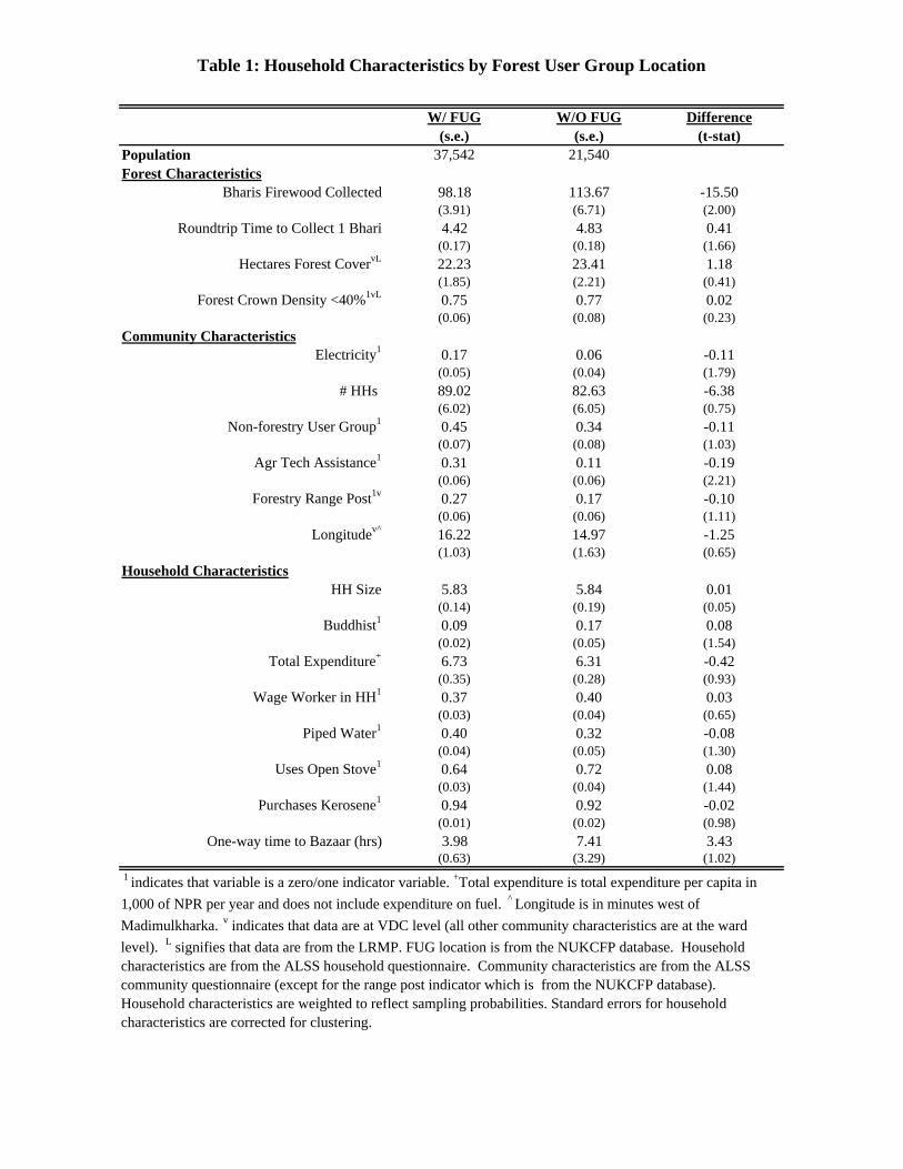
Table 1: Household Characteristics by Forest User Group Location

W/ FUG W/O FUG Difference(s.e.) (s.e.) (t-stat)

Population 37,542 21,540Forest Characteristics

Bharis Firewood Collected 98.18 113.67 -15.50(3.91) (6.71) (2.00)

Roundtrip Time to Collect 1 Bhari 4.42 4.83 0.41(0.17) (0.18) (1.66)

Hectares Forest CovervL 22.23 23.41 1.18(1.85) (2.21) (0.41)

Forest Crown Density <40%1vL 0.75 0.77 0.02(0.06) (0.08) (0.23)

Community CharacteristicsElectricity1 0.17 0.06 -0.11

(0.05) (0.04) (1.79)# HHs 89.02 82.63 -6.38

(6.02) (6.05) (0.75)Non-forestry User Group1 0.45 0.34 -0.11

(0.07) (0.08) (1.03)Agr Tech Assistance1 0.31 0.11 -0.19

(0.06) (0.06) (2.21)Forestry Range Post1v 0.27 0.17 -0.10

(0.06) (0.06) (1.11)Longitudev^ 16.22 14.97 -1.25

(1.03) (1.63) (0.65)Household Characteristics

HH Size 5.83 5.84 0.01(0.14) (0.19) (0.05)

Buddhist1 0.09 0.17 0.08(0.02) (0.05) (1.54)

Total Expenditure+ 6.73 6.31 -0.42(0.35) (0.28) (0.93)

Wage Worker in HH1 0.37 0.40 0.03(0.03) (0.04) (0.65)

Piped Water1 0.40 0.32 -0.08(0.04) (0.05) (1.30)

Uses Open Stove1 0.64 0.72 0.08(0.03) (0.04) (1.44)

Purchases Kerosene1 0.94 0.92 -0.02(0.01) (0.02) (0.98)

One-way time to Bazaar (hrs) 3.98 7.41 3.43(0.63) (3.29) (1.02)

1 indicates that variable is a zero/one indicator variable. +Total expenditure is total expenditure per capita in 1,000 of NPR per year and does not include expenditure on fuel. ^ Longitude is in minutes west of Madimulkharka. v indicates that data are at VDC level (all other community characteristics are at the ward level). L signifies that data are from the LRMP. FUG location is from the NUKCFP database. Household characteristics are from the ALSS household questionnaire. Community characteristics are from the ALSS community questionnaire (except for the range post indicator which is from the NUKCFP database). Household characteristics are weighted to reflect sampling probabilities. Standard errors for household characteristics are corrected for clustering.

Table 2: Forest User Groups and the Fuelwood Collection, Linear Models

I II III IVFUG in Ward -12.65 ** -12.36 ** -10.79 ** -10.26

(3.16) (3.30) (3.12) (3.08)Household CharacteristicsTot Exp Per Cap 0.51 1.39 ** 2.02 **

(0.41) (0.41) (0.44)Owns Agr Land -37.25 ** -28.05 ** -19.73 **

(7.73) (7.30) (7.37)Has Kitchen Garden -9.14 * -11.44 ** -12.11 **

(4.74) (4.49) (4.50)Buddhist 12.14 ** 10.68 ** 14.49 **

(4.91) (4.63) (4.77)Household Size 7.70 ** 7.97 ** 8.10 **

(0.65) (0.64) (0.63)Bonded Walls -2.52 -8.61 ** -8.56 **

(4.31) (4.10) (4.17)Bazaar 1 to 2 hours away 16.61 ** 19.81 ** 18.99 **

(4.07) (3.86) (3.83)Bazaar 2 to 4 hours 12.91 ** 15.73 ** 14.17 **

(4.24) (4.01) (3.96)Bazaar >4 hours 22.91 ** 24.20 ** 22.94 **

(5.28) (4.99) (5.04)Paved Road > 2 hours 47.02 ** 37.87 ** 41.54 **

(11.55) (10.90) (11.11)Piped Water in House -4.22 -7.40 ** -4.35

(3.24) (3.08) (3.11)Uses Open Stove 8.80 **

(3.27)Purchases Kerosene -17.29 **

(5.77)Time to Collect 1 Bhari 1.45 * 1.50 ** 1.62 **

(0.75) (0.74) (0.74)Ward CharacteristicsElectricity in Ward -1.06 -2.82 0.00

(4.52) (4.34) (4.64)Makalu-Barun Ward 13.57 ** 19.87 ** 15.63 **

(6.47) (6.18) (6.22)Alternative Fuel in Ward -29.65 **

(8.20)VDC CharacteristicsForest Area in VDC 0.26 **

(0.11)Tropical Mixed Hardwood Forest 10.18 **

(4.07)Forest w/ Dense Crown -2.87

(4.45)Barren Forest -6.69 *

(3.86)Latitude 2.25 ** 1.29 ** 1.36 ** 1.31 **

(0.17) (0.21) (0.20) (0.24)N 1200 1200 1200 1188Adjusted R2 0.213 0.180 0.276 0.297OLS of bharis collected on various sets of controls. Constant included in regressions. Source : FUG location is from the NUKCFP database. Household characteristics are from the ALSS household questionnaire. Community characteristics are from the ALSS community questionnaire (except for the range post and Makalu-Barun indicators which are from the NUKCFP database). Environmental characteristics are from the LRMP data. Notes : * indicates significant at 10%. ** indicates significant at 5%.

Table 3: Percent Reduction in Fuelwood CollectionConditioning on Observables

I II III IV

Linear Model (eq 4) 11.43 11.24 9.89 9.43(2.65) (2.79) (2.68) (2.66)

Partially Linear Models (eq 5)Flexible Fourier Form

Total Expenditure Per Capita 11.22 9.80 9.47(2.75) (2.73) (2.71)

Collection Time 11.69 10.07 9.26(2.70) (2.69) (2.69)

DifferencingTotal Expenditure Per Capita 9.91 8.36 8.36

(2.91) (2.86) (2.87)

Collection Time 14.47 11.54 12.39(3.02) (3.05) (3.11)

Flexible Linear Model (eq 6) 12.42 10.35 10.73 9.27(2.64) (2.92) (2.73) (2.90)

Kernel Matching ModelsUnivariate Matching

Total Expenditure 12.77(6.24)

Collection Time 12.38(6.34)

Matching on Set I. 10.02(6.54)

Estimates in the top panel are based on dividing the reduction in firewood collection with forest groups by the predicted firewood collection absent forest groups for those areas with forest groups. In rows 1 and 2, standard errors are calculcated by application of the delta method. The regression variance covariance matrix in partially linear models is bootstrapped using a clustered bootstrap with 1,000 replications. Matching estimators use a Gaussian Kernel with bandwidth selection by Silverman (1986): p48 for univariate matching, p 87 for multivariate matching. Standard errors for the matching estimators are bootstrapped with a clustered bootstrap, 1,000 replications.

Table 4: Percent Reduction in Fuelwood CollectionOmitted Variable Strategies

Relative to Areas Receiving User Groups After Survey Time

Sample Mean 32.95(17.80)

Linear Regression Model (eq 8) 24.94(5.69)

Instrumental Variables Results

IV-2SLS (eq 4) 22.54(8.58)

IV-2SLS (eq 6) 23.19(8.32)

The top panel compares areas that receive forest user groups in the year prior to the survey with areas that receive forest groups in the year after the survey. A forest group indicator, total expenditure per capita, roundtrip time to collect 1 bhari of firewood, household size, latitude, and a constant are included in all regressions . The bottom panel contains instrumental variables results. The first row contains two stage least squares estimates of the coefficient on the forest user group indicator. Instruments are indicators for if there is a range post in the VDC, other non-forestry user groups in the ward, or agricultural technical assistance in the ward. Row 2 allows the controls to interact with the instrumented forest user group indicator. Standard errors are derived using the delta-method. All estimates are significant at the 5% level.

Table 5:FUG Formation After the Household Survey, Probit Results

dF/dX S.E. dF/dX S.E. dF/dX S.E. dF/dX S.E.

Household CharacteristicsTot Exp Per Cap -0.003 0.002 -0.003 0.002 -0.003 0.002 0.003 0.001 **

Wage Worker in HH -0.023 0.010 **

Owns Agr Land 0.066 0.020 **

Has Kitchen Garden 0.007 0.012Buddhist 0.020 0.018Household Size 0.009 0.003 ** 0.007 0.003 ** 0.007 0.003 ** 0.009 0.003 **

# Adults -0.005 0.004Bonded Walls -0.033 0.019 **

Bazaar 1 to 2 hours away 0.042 0.019 **

Bazaar 2 to 4 hours 0.026 0.018 *

Bazaar >4 hours 0.055 0.031 **

Paved Road > 2 hours 0.319 0.120 **

Piped Water in House -0.011 0.010Roundtrip Time to Collect 1 Bhari -0.023 0.004 ** -0.023 0.004 ** -0.023 0.004 ** -0.006 0.003 **

Bharis Collected 0.000 0.000 0.000 0.000 0.000 0.000

Ward CharacteristicsElectricity in Ward -0.028 0.008 **

Other User Group in Ward -0.061 0.016 ** -0.061 0.016 ** -0.061 0.016 ** -0.033 0.010 **

Agr Tech Assistance in Ward -0.106 0.013 ** -0.105 0.013 ** -0.106 0.013 ** -0.057 0.009 **

Forest User Group in Ward 0.007 0.016 0.003 0.011

VDC CharacteristicsForest Area in VDC 0.001 0.000 **

# Dominant Tree Species -0.019 0.008 **

Tropical Mixed Hardwood Forest 0.063 0.009 **

Forest w/ Dense Crown -0.045 0.009 **

Barren Forest -0.151 0.041 **

Range Post in VDC 0.213 0.031 ** 0.214 0.031 ** 0.213 0.031 ** 0.184 0.032 **

Longitude -0.008 0.001 **

Latitude 0.004 0.001 ** 0.003 0.001 ** 0.003 0.001 ** 0.002 0.001 *

N 1200 1200 1200 1188

Pseudo R2 0.1896 0.1914 0.1915 0.3824

Coefficients are probit results evaluated at the sample mean. For indicator variables, the coefficients are evaluated at a change from 0 to 1. A constant was included in the regression. The dependent variable is an indicator for if a forest user group forms in the ward after the survey is completed. This can include both wards without a forest user group at survey time and wards that receive an additional forest user group after the survey. * indicates significant at 10%. ** indicates significant at 5%.

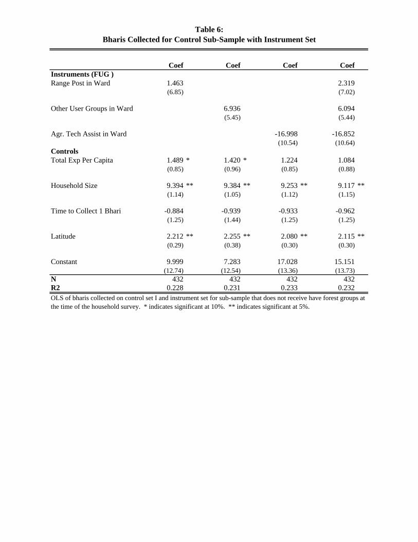
Table 6:Bharis Collected for Control Sub-Sample with Instrument Set

Coef Coef Coef CoefInstruments (FUG )Range Post in Ward 1.463 2.319

(6.85) (7.02)

Other User Groups in Ward 6.936 6.094(5.45) (5.44)

Agr. Tech Assist in Ward -16.998 -16.852(10.54) (10.64)

ControlsTotal Exp Per Capita 1.489 * 1.420 * 1.224 1.084

(0.85) (0.96) (0.85) (0.88)

Household Size 9.394 ** 9.384 ** 9.253 ** 9.117 **(1.14) (1.05) (1.12) (1.15)

Time to Collect 1 Bhari -0.884 -0.939 -0.933 -0.962(1.25) (1.44) (1.25) (1.25)

Latitude 2.212 ** 2.255 ** 2.080 ** 2.115 **(0.29) (0.38) (0.30) (0.30)

Constant 9.999 7.283 17.028 15.151(12.74) (12.54) (13.36) (13.73)

N 432 432 432 432R2 0.228 0.231 0.233 0.232OLS of bharis collected on control set I and instrument set for sub-sample that does not receive have forest groups at the time of the household survey. * indicates significant at 10%. ** indicates significant at 5%.