buildingblocks for theoreticalcomputerscience...
TRANSCRIPT

Building Blocksfor
Theoretical Computer Science(preliminary version 1.0)
Margaret M. Fleck
January 9, 2012
Contents
Preface xi
1 Math review 1
1.1 Some sets . . . . . . . . . . . . . . . . . . . . . . . . . . . . . 1
1.2 Pairs of reals . . . . . . . . . . . . . . . . . . . . . . . . . . . 3
1.3 Exponentials and logs . . . . . . . . . . . . . . . . . . . . . . 4
1.4 Factorial, floor, and ceiling . . . . . . . . . . . . . . . . . . . . 5
1.5 Summations . . . . . . . . . . . . . . . . . . . . . . . . . . . . 6
1.6 Variation in notation . . . . . . . . . . . . . . . . . . . . . . . 8
2 Logic 9
2.1 A bit about style . . . . . . . . . . . . . . . . . . . . . . . . . 9
2.2 Propositions . . . . . . . . . . . . . . . . . . . . . . . . . . . . 10
2.3 Complex propositions . . . . . . . . . . . . . . . . . . . . . . . 10
2.4 Implication . . . . . . . . . . . . . . . . . . . . . . . . . . . . 11
2.5 Converse, contrapositive, biconditional . . . . . . . . . . . . . 13
2.6 Complex statements . . . . . . . . . . . . . . . . . . . . . . . 14
2.7 Logical Equivalence . . . . . . . . . . . . . . . . . . . . . . . . 15
2.8 Some useful logical equivalences . . . . . . . . . . . . . . . . . 16
i
CONTENTS ii
2.9 Negating propositions . . . . . . . . . . . . . . . . . . . . . . . 17
2.10 Predicates and Variables . . . . . . . . . . . . . . . . . . . . . 18
2.11 Other quantifiers . . . . . . . . . . . . . . . . . . . . . . . . . 19
2.12 Notation . . . . . . . . . . . . . . . . . . . . . . . . . . . . . . 20
2.13 Useful notation . . . . . . . . . . . . . . . . . . . . . . . . . . 21
2.14 Notation for 2D points . . . . . . . . . . . . . . . . . . . . . . 22
2.15 Negating statements with quantifiers . . . . . . . . . . . . . . 23
2.16 Binding and scope . . . . . . . . . . . . . . . . . . . . . . . . 24
2.17 Variations in Notation . . . . . . . . . . . . . . . . . . . . . . 24
3 Proofs 26
3.1 Proving a universal statement . . . . . . . . . . . . . . . . . . 26
3.2 Another example of direct proof involving odd and even . . . . 28
3.3 Direct proof outline . . . . . . . . . . . . . . . . . . . . . . . . 29
3.4 Proving existential statements . . . . . . . . . . . . . . . . . . 30
3.5 Disproving a universal statement . . . . . . . . . . . . . . . . 30
3.6 Disproving an existential statement . . . . . . . . . . . . . . . 31
3.7 Recap of proof methods . . . . . . . . . . . . . . . . . . . . . 32
3.8 Direct proof: example with two variables . . . . . . . . . . . . 32
3.9 Another example with two variables . . . . . . . . . . . . . . . 33
3.10 Proof by cases . . . . . . . . . . . . . . . . . . . . . . . . . . . 34
3.11 Rephrasing claims . . . . . . . . . . . . . . . . . . . . . . . . . 35
3.12 Proof by contrapositive . . . . . . . . . . . . . . . . . . . . . . 36
3.13 Another example of proof by contrapositive . . . . . . . . . . 37
3.14 Proof by contradiction . . . . . . . . . . . . . . . . . . . . . . 38
3.15√2 is irrational . . . . . . . . . . . . . . . . . . . . . . . . . . 38
CONTENTS iii
4 Number Theory 40
4.1 Factors and multiples . . . . . . . . . . . . . . . . . . . . . . . 40
4.2 Direct proof with divisibility . . . . . . . . . . . . . . . . . . . 41
4.3 Stay in the Set . . . . . . . . . . . . . . . . . . . . . . . . . . 42
4.4 Prime numbers . . . . . . . . . . . . . . . . . . . . . . . . . . 43
4.5 There are infinitely many prime numbers . . . . . . . . . . . . 43
4.6 GCD and LCM . . . . . . . . . . . . . . . . . . . . . . . . . . 44
4.7 The division algorithm . . . . . . . . . . . . . . . . . . . . . . 45
4.8 Euclidean algorithm . . . . . . . . . . . . . . . . . . . . . . . 46
4.9 Pseudocode . . . . . . . . . . . . . . . . . . . . . . . . . . . . 47
4.10 A recursive version of gcd . . . . . . . . . . . . . . . . . . . . 48
4.11 Congruence mod k . . . . . . . . . . . . . . . . . . . . . . . . 48
4.12 Proofs with congruence mod k . . . . . . . . . . . . . . . . . . 50
4.13 Equivalence classes . . . . . . . . . . . . . . . . . . . . . . . . 50
4.14 Wider perspective on equivalence . . . . . . . . . . . . . . . . 52
4.15 Variation in Terminology . . . . . . . . . . . . . . . . . . . . . 53
5 Sets 54
5.1 Sets . . . . . . . . . . . . . . . . . . . . . . . . . . . . . . . . 54
5.2 Things to be careful about . . . . . . . . . . . . . . . . . . . . 55
5.3 Cardinality, inclusion . . . . . . . . . . . . . . . . . . . . . . . 56
5.4 Vacuous truth . . . . . . . . . . . . . . . . . . . . . . . . . . . 57
5.5 Set operations . . . . . . . . . . . . . . . . . . . . . . . . . . . 58
5.6 Set identities . . . . . . . . . . . . . . . . . . . . . . . . . . . 59
5.7 Size of set union . . . . . . . . . . . . . . . . . . . . . . . . . . 60
5.8 Product rule . . . . . . . . . . . . . . . . . . . . . . . . . . . . 61

CONTENTS iv
5.9 Combining these basic rules . . . . . . . . . . . . . . . . . . . 62
5.10 Proving facts about set inclusion . . . . . . . . . . . . . . . . 63
5.11 Example proof: deMorgan’s law . . . . . . . . . . . . . . . . . 64
5.12 An example with products . . . . . . . . . . . . . . . . . . . . 64
5.13 Another example with products . . . . . . . . . . . . . . . . . 65
5.14 A proof using sets and contrapositive . . . . . . . . . . . . . . 67
5.15 Variation in notation . . . . . . . . . . . . . . . . . . . . . . . 67
6 Relations 68
6.1 Relations . . . . . . . . . . . . . . . . . . . . . . . . . . . . . . 68
6.2 Properties of relations: reflexive . . . . . . . . . . . . . . . . . 70
6.3 Symmetric and antisymmetric . . . . . . . . . . . . . . . . . . 71
6.4 Transitive . . . . . . . . . . . . . . . . . . . . . . . . . . . . . 72
6.5 Types of relations . . . . . . . . . . . . . . . . . . . . . . . . . 74
6.6 Proving that a relation is an equivalence relation . . . . . . . . 75
6.7 Proving antisymmetry . . . . . . . . . . . . . . . . . . . . . . 76
7 Functions and onto 77
7.1 Functions . . . . . . . . . . . . . . . . . . . . . . . . . . . . . 77
7.2 When are functions equal? . . . . . . . . . . . . . . . . . . . . 79
7.3 What isn’t a function? . . . . . . . . . . . . . . . . . . . . . . 80
7.4 Images and Onto . . . . . . . . . . . . . . . . . . . . . . . . . 80
7.5 Why are some functions not onto? . . . . . . . . . . . . . . . . 81
7.6 Negating onto . . . . . . . . . . . . . . . . . . . . . . . . . . . 82
7.7 Nested quantifiers . . . . . . . . . . . . . . . . . . . . . . . . . 83
7.8 Proving that a function is onto . . . . . . . . . . . . . . . . . 85

CONTENTS v
7.9 A 2D example . . . . . . . . . . . . . . . . . . . . . . . . . . . 86
7.10 Composing two functions . . . . . . . . . . . . . . . . . . . . . 86
7.11 A proof involving composition . . . . . . . . . . . . . . . . . . 87
7.12 Variation in terminology . . . . . . . . . . . . . . . . . . . . . 88
8 Functions and one-to-one 89
8.1 One-to-one . . . . . . . . . . . . . . . . . . . . . . . . . . . . . 89
8.2 Bijections . . . . . . . . . . . . . . . . . . . . . . . . . . . . . 91
8.3 Pigeonhole Principle . . . . . . . . . . . . . . . . . . . . . . . 91
8.4 Permutations . . . . . . . . . . . . . . . . . . . . . . . . . . . 93
8.5 Further applications of permutations . . . . . . . . . . . . . . 94
8.6 Proving that a function is one-to-one . . . . . . . . . . . . . . 95
8.7 Composition and one-to-one . . . . . . . . . . . . . . . . . . . 95
8.8 Strictly increasing functions are one-to-one . . . . . . . . . . . 97
8.9 Making this proof more succinct . . . . . . . . . . . . . . . . . 98
8.10 Variation in terminology . . . . . . . . . . . . . . . . . . . . . 99
9 Graphs 100
9.1 Graphs . . . . . . . . . . . . . . . . . . . . . . . . . . . . . . . 100
9.2 Degrees . . . . . . . . . . . . . . . . . . . . . . . . . . . . . . 102
9.3 Complete graphs . . . . . . . . . . . . . . . . . . . . . . . . . 103
9.4 Cycle graphs and wheels . . . . . . . . . . . . . . . . . . . . . 104
9.5 Isomorphism . . . . . . . . . . . . . . . . . . . . . . . . . . . . 105
9.6 Subgraphs . . . . . . . . . . . . . . . . . . . . . . . . . . . . . 106
9.7 Walks, paths, and cycles . . . . . . . . . . . . . . . . . . . . . 107
9.8 Connectivity . . . . . . . . . . . . . . . . . . . . . . . . . . . . 109
CONTENTS vi
9.9 Distances . . . . . . . . . . . . . . . . . . . . . . . . . . . . . 110
9.10 Euler circuits . . . . . . . . . . . . . . . . . . . . . . . . . . . 110
9.11 Graph coloring . . . . . . . . . . . . . . . . . . . . . . . . . . 111
9.12 Why should I care? . . . . . . . . . . . . . . . . . . . . . . . . 113
9.13 Bipartite graphs . . . . . . . . . . . . . . . . . . . . . . . . . . 114
9.14 Variation in terminology . . . . . . . . . . . . . . . . . . . . . 115
10 Induction 117
10.1 Introduction to induction . . . . . . . . . . . . . . . . . . . . . 117
10.2 An Example . . . . . . . . . . . . . . . . . . . . . . . . . . . . 118
10.3 Why is this legit? . . . . . . . . . . . . . . . . . . . . . . . . . 119
10.4 Building an inductive proof . . . . . . . . . . . . . . . . . . . 121
10.5 Another example of induction . . . . . . . . . . . . . . . . . . 121
10.6 Some comments about style . . . . . . . . . . . . . . . . . . . 123
10.7 Another example . . . . . . . . . . . . . . . . . . . . . . . . . 123
10.8 A geometrical example . . . . . . . . . . . . . . . . . . . . . . 124
10.9 Graph coloring . . . . . . . . . . . . . . . . . . . . . . . . . . 126
10.10Postage example . . . . . . . . . . . . . . . . . . . . . . . . . 128
10.11Nim . . . . . . . . . . . . . . . . . . . . . . . . . . . . . . . . 129
10.12Prime factorization . . . . . . . . . . . . . . . . . . . . . . . . 130
10.13Variation in notation . . . . . . . . . . . . . . . . . . . . . . . 131
11 Recursive Definition 133
11.1 Recursive definitions . . . . . . . . . . . . . . . . . . . . . . . 133
11.2 Finding closed forms . . . . . . . . . . . . . . . . . . . . . . . 134
11.3 Divide and conquer . . . . . . . . . . . . . . . . . . . . . . . . 136
CONTENTS vii
11.4 Hypercubes . . . . . . . . . . . . . . . . . . . . . . . . . . . . 138
11.5 Proofs with recursive definitions . . . . . . . . . . . . . . . . . 139
11.6 Inductive definition and strong induction . . . . . . . . . . . . 140
11.7 Variation in notation . . . . . . . . . . . . . . . . . . . . . . . 141
12 Trees 142
12.1 Why trees? . . . . . . . . . . . . . . . . . . . . . . . . . . . . 142
12.2 Defining trees . . . . . . . . . . . . . . . . . . . . . . . . . . . 145
12.3 m-ary trees . . . . . . . . . . . . . . . . . . . . . . . . . . . . 146
12.4 Height vs number of nodes . . . . . . . . . . . . . . . . . . . . 147
12.5 Context-free grammars . . . . . . . . . . . . . . . . . . . . . . 147
12.6 Recursion trees . . . . . . . . . . . . . . . . . . . . . . . . . . 151
12.7 Another recursion tree example . . . . . . . . . . . . . . . . . 153
12.8 Tree induction . . . . . . . . . . . . . . . . . . . . . . . . . . . 154
12.9 Heap example . . . . . . . . . . . . . . . . . . . . . . . . . . . 155
12.10Proof using grammar trees . . . . . . . . . . . . . . . . . . . . 157
12.11Variation in terminology . . . . . . . . . . . . . . . . . . . . . 158
13 Big-O 160
13.1 Running times of programs . . . . . . . . . . . . . . . . . . . . 160
13.2 Function growth: the ideas . . . . . . . . . . . . . . . . . . . . 161
13.3 Primitive functions . . . . . . . . . . . . . . . . . . . . . . . . 162
13.4 The formal definition . . . . . . . . . . . . . . . . . . . . . . . 164
13.5 Applying the definition . . . . . . . . . . . . . . . . . . . . . . 164
13.6 Writing a big-O proof . . . . . . . . . . . . . . . . . . . . . . . 165
13.7 Sample disproof . . . . . . . . . . . . . . . . . . . . . . . . . . 166

CONTENTS viii
13.8 Variation in notation . . . . . . . . . . . . . . . . . . . . . . . 166
14 Algorithms 168
14.1 Introduction . . . . . . . . . . . . . . . . . . . . . . . . . . . . 168
14.2 Basic data structures . . . . . . . . . . . . . . . . . . . . . . . 168
14.3 Nested loops . . . . . . . . . . . . . . . . . . . . . . . . . . . . 170
14.4 Merging two lists . . . . . . . . . . . . . . . . . . . . . . . . . 171
14.5 A reachability algorithm . . . . . . . . . . . . . . . . . . . . . 172
14.6 Binary search . . . . . . . . . . . . . . . . . . . . . . . . . . . 173
14.7 Mergesort . . . . . . . . . . . . . . . . . . . . . . . . . . . . . 175
14.8 Tower of Hanoi . . . . . . . . . . . . . . . . . . . . . . . . . . 176
14.9 Multiplying big integers . . . . . . . . . . . . . . . . . . . . . 178
15 Sets of Sets 181
15.1 Sets containing sets . . . . . . . . . . . . . . . . . . . . . . . . 181
15.2 Powersets and set-valued functions . . . . . . . . . . . . . . . 182
15.3 Partitions . . . . . . . . . . . . . . . . . . . . . . . . . . . . . 184
15.4 Combinations . . . . . . . . . . . . . . . . . . . . . . . . . . . 186
15.5 Applying the combinations formula . . . . . . . . . . . . . . . 187
15.6 Combinations with repetition . . . . . . . . . . . . . . . . . . 188
15.7 Identities for binomial coefficients . . . . . . . . . . . . . . . . 189
15.8 Binomial Theorem . . . . . . . . . . . . . . . . . . . . . . . . 190
15.9 Variation in notation . . . . . . . . . . . . . . . . . . . . . . . 191
16 State Diagrams 192
16.1 Introduction . . . . . . . . . . . . . . . . . . . . . . . . . . . . 192
16.2 Wolf-goat-cabbage puzzle . . . . . . . . . . . . . . . . . . . . . 194
CONTENTS ix
16.3 Phone lattices . . . . . . . . . . . . . . . . . . . . . . . . . . . 195
16.4 Representing functions . . . . . . . . . . . . . . . . . . . . . . 196
16.5 Transition functions . . . . . . . . . . . . . . . . . . . . . . . . 197
16.6 Shared states . . . . . . . . . . . . . . . . . . . . . . . . . . . 198
16.7 Counting states . . . . . . . . . . . . . . . . . . . . . . . . . . 200
16.8 Variation in notation . . . . . . . . . . . . . . . . . . . . . . . 201
17 Countability 202
17.1 The rationals and the reals . . . . . . . . . . . . . . . . . . . . 202
17.2 Completeness . . . . . . . . . . . . . . . . . . . . . . . . . . . 203
17.3 Cardinality . . . . . . . . . . . . . . . . . . . . . . . . . . . . 203
17.4 More countably infinite sets . . . . . . . . . . . . . . . . . . . 204
17.5 Cantor Schroeder Bernstein Theorem . . . . . . . . . . . . . . 205
17.6 P(N) isn’t countable . . . . . . . . . . . . . . . . . . . . . . . 206
17.7 More uncountability results . . . . . . . . . . . . . . . . . . . 207
17.8 Uncomputability . . . . . . . . . . . . . . . . . . . . . . . . . 208
17.9 Variation in notation . . . . . . . . . . . . . . . . . . . . . . . 209
18 Planar Graphs 210
18.1 Planar graphs . . . . . . . . . . . . . . . . . . . . . . . . . . . 210
18.2 Faces . . . . . . . . . . . . . . . . . . . . . . . . . . . . . . . . 211
18.3 Trees . . . . . . . . . . . . . . . . . . . . . . . . . . . . . . . . 212
18.4 Proof of Euler’s formula . . . . . . . . . . . . . . . . . . . . . 213
18.5 Some corollaries of Euler’s formula . . . . . . . . . . . . . . . 214
18.6 K3,3 is not planar . . . . . . . . . . . . . . . . . . . . . . . . . 215
18.7 Kuratowski’s Theorem . . . . . . . . . . . . . . . . . . . . . . 216

CONTENTS x
18.8 Coloring planar graphs . . . . . . . . . . . . . . . . . . . . . . 219
18.9 Application: Platonic solids . . . . . . . . . . . . . . . . . . . 220
A Jargon 223
A.1 Strange technical terms . . . . . . . . . . . . . . . . . . . . . . 223
A.2 Odd uses of normal words . . . . . . . . . . . . . . . . . . . . 224
A.3 Constructions . . . . . . . . . . . . . . . . . . . . . . . . . . . 226
A.4 Unexpectedly normal . . . . . . . . . . . . . . . . . . . . . . . 227
B Acknowledgements and Supplementary Readings 228

Preface
This book teaches two different sorts of things, woven together. It teachesyou how to read and write mathematical proofs. It also provides a surveyof basic mathematical objects, notation, and techniques which will be usefulin later computer science courses. These include propositional and predicatelogic, sets, functions, relations, modular arithmetic, counting, graphs, andtrees.
Why learn formal mathematics?
Formal mathematics is relevant to computer science in several ways. First, itis used to create theoretical designs for algorithms and prove that they workcorrectly. This is especially important for methods that are used frequentlyand/or in applications where we don’t want failures (aircraft design, Pentagonsecurity, ecommerce). Only some people do these designs, but many peopleuse them. The users need to be able to read and understand how the designswork.
Second, the skills you learn in doing formal mathematics correspondclosely to those required to design and debug programs. Both require keepingtrack of what types your variables are. Both use inductive and/or recursivedesign. And both require careful proofreading skills. So what you learn inthis class will also help you succeed in practical programming courses.
Third, when you come to design complex real software, you’ll have todocument what you’ve done and how it works. This is hard for many peo-ple to do well, but it’s critical for the folks using your software. Learninghow to describe mathematical objects clearly will translate into better skills
xi
PREFACE xii
describing computational objects.
Everyone can do proofs
You probably think about proofs as something created by brilliant youngtheoreticians. Some of you are brilliant young theoreticians and you’ll thinkthis stuff is fun because it’s what you naturally like to do. However, manyof you are future software and hardware engineers. Some of you may neverthink of formal mathematics as “fun.” That’s ok. We understand. We’rehoping to give you a sense of why it’s pretty and useful, and enough fluencywith it to communicate with the theoretical side of the field.
Many people think that proofs involve being incredibly clever. That istrue for some steps in some proofs. That’s where it helps to actually be abrilliant young theoretician. But many proofs are very routine. And manysteps in clever proofs are routine. So there’s quite a lot of proofs that all ofus can do. And we can all read, understand, and appreciate the clever bitsthat we didn’t think up ourselves.
In other words, don’t be afraid. You can do proofs at the level requiredfor this course, and future courses in theoretical computer science.
Is this book right for you?
This book is designed for students who have taken an introductory program-ming class of the sort intended for scientists or engineers. Algorithms willbe presented in “pseudo-code,” so it does not matter which programminglanguage you have used. But you should have written programs that ma-nipulate the contents of arrays e.g. sort an array of numbers. You shouldalso have written programs that are recursive, i.e. in which a function (akaprocedure aka method) calls itself.
We’ll also assume that you have taken one semester of calculus. Thoughwe will make little direct reference to calculus, we will assume a level of flu-ency with precalculus (algebra, geometry, logarithms, etc) that is typicallydeveloped during while taking calculus. If you already have significant expe-
PREFACE xiii
rience writing proofs, including inductive proofs, this book may be too easyfor you. You may wish to read some of the books listed as supplementaryreadings in Appendix B.
For instructors
This text is designed for a broad range of computer science majors, rangingfrom budding young theoreticians to capable programmers with very littleinterest in theory. It assumes only limited mathematical maturity, so that itcan be used very early in the major. Therefore, a central goal is to explainthe process of proof construction clearly to students who can’t just pick itup by osmosis.
This book is designed to be succinct, so that students will read and absorbits contents. Therefore, it includes only core concepts and a selection ofillustrative examples, with the expectation that the instructor will providesupplementary materials as needed and that students can look up a widerrange of facts, definitions, and pictures, e.g. on the internet.
Although the core topics in this book are old and established, terminol-ogy and notation have changed over the years and vary somewhat betweenauthors. To avoid overloading students, I have chosen one clean, modernversion of notation, definitions, and terminology to use consistently in themain text. Common variations are documented at the end of each chapter. Ifstudents understand the underlying concepts, they should have no difficultyadapting when they encounter different conventions in other books.
Many traditional textbooks do a careful and exhaustive treatment of eachtopic from first principles, including foundational constructions and theoremswhich prove that the conceptual system is well-formed. However, the mostabstract parts of many topics are hard for beginners to absorb and the impor-tance of the foundational development is lost on most students at this level.The early parts of this textbook remove most of this clutter, to focus moreclearly on the key concepts and constructs. At the end, we revisit certaintopics to look at more abstract examples and selected foundational issues.
Chapter 1
Math review
This book assumes that you understood precalculus when you took it. So youused to know how to do things like factoring polynomials, solving high schoolgeometry problems, using trigonometric identities. However, you probablycan’t remember it all cold. Many useful facts can be looked up (e.g. on theinternet) as you need them. This chapter reviews concepts and notation thatwill be used a lot in this book, as well as a few concepts that may be newbut are fairly easy.
1.1 Some sets
You’ve all seen sets, though probably a bit informally. We’ll get back to someof the formalism in a couple weeks. Meanwhile, here are the names for a fewcommonly used sets of numbers:
• Z = {. . . ,−3,−2,−1, 0, 1, 2, 3, . . .} is the integers.
• N = {0, 1, 2, 3, . . .} is the non-negative integers, also known as thenatural numbers.
• Z+ = {1, 2, 3, . . .} is the positive integers.
• R is the real numbers
1
CHAPTER 1. MATH REVIEW 2
• Q is the rational numbers
• C is the complex numbers
Notice that a number is positive if it is greater than zero, so zero is notpositive. If you wish to exclude negative values, but include zero, you mustuse the term “non-negative.” In this book, natural numbers are defined toinclude zero.
Remember that the rational numbers are the set of fractions p
qwhere q
can’t be zero and we consider two fractions to be the same number if theyare the same when you reduce them to lowest terms.
The real numbers contain all the rationals, plus irrational numbers suchas
√2 and π. (Also e, but we don’t use e much in this end of computer
science.) We’ll assume that√x returns (only) the positive square root of x.
The complex numbers are numbers of the form a+ bi, where a and b arereal numbers and i is the square root of -1. Some of you from ECE will beaware that there are many strange and interesting things that can be donewith the complex numbers. We won’t be doing that here. We’ll just usethem for a few examples and expect you to do very basic things, mostly easyconsequences of the fact that i =
√−1.
If we want to say that the variable x is a real, we write x ∈ R. Similarlyy 6∈ Z means that y is not an integer. In calculus, you don’t have to thinkmuch about the types of your variables, because they are largely reals. Inthis class, we handle variables of several different types, so it’s important tostate the types explicitly.
It is sometimes useful to select the real numbers in some limited range,called an interval of the real line. We use the following notation:
• closed interval: [a, b] is the set of real numbers from a to b, including aand b
• open interval: (a, b) is the set of real numbers from a to b, not includinga and b
• half-open intervals: [a, b) and (a, b] include only one of the two end-points.

CHAPTER 1. MATH REVIEW 3
1.2 Pairs of reals
The set of all pairs of reals is written R2. So it contains pairs like (−2.3, 4.7).In a computer program, we implement a pair of reals using an object or structwith two fields.
Suppose someone presents you with a pair of numbers (x, y) or one of thecorresponding data structures. Your first question should be: what is thepair intended to represent? It might be
• a point in 2D space
• a complex number
• a rational number (if the second coordinate isn’t zero)
• an interval of the real line
The intended meaning affects what operations we can do on the pairs.For example, if (x, y) is an interval of the real line, it’s a set. So we can writethings like z ∈ (x, y) meaning z is in the interval (x, y). That notation wouldbe meaningless if (x, y) is a 2D point or a number.
If the pairs are numbers, we can add them, but the result depends onwhat they are representing. So (x, y) + (a, b) is (x + a, y + b) for 2D pointsand complex numbers. But it is (xb+ ya, yb) for rationals.
Suppose we want to multiply (x, y)×(a, b) and get another pair as output.There’s no obvious way to do this for 2D points. For rationals, the formulawould be (xa, yb), but for complex numbers it’s (xa− yb, ya+ xb).
Stop back and work out that last one for the non-ECE students, usingmore familiar notation. (x+yi)(a+ bi) is xa+yai+xbi+ byi2. But i2 = −1.So this reduces to (xa− yb) + (ya+ xb)i.
Oddly enough, you can also multiply two intervals of the real line. Thiscarves out a rectangular region of the 2D plane, with sides determined bythe two intervals.

CHAPTER 1. MATH REVIEW 4
1.3 Exponentials and logs
Suppose that b is any real number. We all know how to take integer powersof b, i,e. bn is b multiplied by itself n times. It’s not so clear how to preciselydefine bx, but we’ve all got faith that it works (e.g. our calculators producevalues for it) and it’s a smooth function that grows really fast as the inputgets bigger and agrees with the integer definition on integer inputs.
Here are some special cases to know
• b0 is one for any b.
• b0.5 is√b
• b−1 is 1b
And some handy rules for manipulating exponents:
bxby = bx+y
axbx = (ab)x
(bx)y = bxy
b(xy) 6= (bx)y
Suppose that b > 1. Then we can invert the function bx, to get the func-tion logb x (“logarithm of x to the base b”). Logarithms appear in computerscience as the running times of particularly fast algorithms. They are alsoused to manipulate numbers that have very wide ranges, e.g. probabilities.Notice that the log function takes only positive numbers as inputs. In thisclass, log x with no explicit base always means log2 x because analysis ofcomputer algorithms makes such heavy use of base-2 numbers and powers of2.
Useful facts about logarithms include:
CHAPTER 1. MATH REVIEW 5
blogb(x) = x
logb(xy) = logb x+ logb y
logb(xy) = y logb x
logb x = loga x logb a
In the change of base formula, it’s easy to forget whether the last termshould be logb a or loga b. To figure this out on the fly, first decide which oflogb x and loga x is larger. You then know whether the last term should belarger or smaller than one. One of logb a and loga b is larger than one andthe other is smaller: figure out which is which.
More importantly, notice that the multiplier to change bases is a con-stant, i.e doesn’t depend on x. So it just shifts the curve up and downwithout really changing its shape. That’s an extremely important fact thatyou should remember, even if you can’t reconstruct the precise formula. Inmany computer science analyses, we don’t care about constant multipliers.So the fact that base changes simply multiply by a constant means that wefrequently don’t have to care what the base actually is. Thus, authors oftenwrite log x and don’t specify the base.
1.4 Factorial, floor, and ceiling
The factorial function may or may not be familiar to you, but is easy toexplain. Suppose that k is any positive integer. Then k factorial, written k!,is the product of all the positive integers up to and including k. That is
k! = 1 · 2 · 3 · . . . · (k − 1) · k
For example, 5! = 1 · 2 · 3 · 4 · 5 = 120. 0! is defined to be 1.
The floor and ceiling functions are heavily used in computer science,though not in many areas other of science and engineering. Both functionstake a real number x as input and return an integer near x. The floor func-tion returns the largest integer no bigger than x. In other words, it converts

CHAPTER 1. MATH REVIEW 6
x to an integer, rounding down. This is written ⌊x⌋. If the input to flooris already an integer, it is returned unchanged. Notice that floor roundsdownward even for negative numbers. So:
⌊3.75⌋ = 3
⌊3⌋ = 3
⌊−3.75⌋ = −4
The ceiling function, written ⌈x⌉, is similar, but rounds upwards. Forexample:
⌈3.75⌉ = 4
⌈3⌉ = 3
⌈−3.75⌉ = −3
Most programming languages have these two functions, plus a functionthat rounds to the nearest integer and one that “truncates” i.e. roundstowards zero. Round is often used in statistical programs. Truncate isn’tused much in theoretical analyses.
1.5 Summations
If ai is some formula that depends on i, then
n∑
i=1
ai = a1 + a2 + a3 + . . .+ an
For example
n∑
i=1
1
2i=
1
2+
1
4+
1
8. . .+
1
2n
Products can be written with a similar notation, e.g.

CHAPTER 1. MATH REVIEW 7
n∏
k=1
1
k=
1
1· 12· 13· . . . · 1
n
Certain sums can be re-expressed “in closed form” i.e. without the sum-mation notation. For example:
n∑
i=1
1
2i= 1− 1
2n
In Calculus, you may have seen the infinite version of this sum, whichconverges to 1. In this class, we’re always dealing with finite sums, notinfinite ones.
If you modify the start value, so we start with the zeroth term, we getthe following variation on this summation. Always be careful to check whereyour summation starts.
n∑
i=0
1
2i= 2− 1
2n
Many reference books have tables of useful formulas for summations thathave simple closed forms. We’ll see them again when we cover mathematicalinduction and see how to formally prove that they are correct.
Only a very small number of closed forms need to be memorized. Oneexample is
n∑
i=1
i =n(n+ 1)
2
Here’s one way to convince yourself it’s right. On graph paper, draw abox n units high and n+1 units wide. Its area is n(n+1). Fill in the leftmostpart of each row to represent one term of the summation: the left box in thefirst row, the left two boxes in the second row, and so on. This makes a littletriangular pattern which fills exactly half the box.

CHAPTER 1. MATH REVIEW 8
1.6 Variation in notation
Mathematical notation is not entirely standardized and has changed over theyears, so you will find that different subfields and even different individualauthors use slightly different notation. These “variation in notation” sectionstell you about synonyms and changes in notation that you are very likely toencounter elsewhere. Always check carefully which convention an author isusing. When doing problems on homework or exams for a class, follow thehouse style used in that particular class.
In particular, authors differ as to whether zero is in the natural numbers.Moreover,
√−1 is named j over in ECE and physics, because i is used for
current. Outside of computer science, the default base for logarithms isusually e, because this makes a number of continuous mathematical formulaswork nicely (just as base 2 makes many computer science formulas worknicely).
Chapter 2
Logic
This chapter covers propositional logic and predicate logic at a basic level.Some deeper issues will be covered later.
2.1 A bit about style
Writing mathematics requires two things. You need to get the logical flow ofideas correct. And you also need to express yourself in standard style, in away that is easy for humans (not computers) to read. Mathematical style isbest taught by example and is similar to what happens in English classes.
Mathematical writing uses a combination of equations and also parts thatlook superficially like English. Mathematical English is almost like normalEnglish, but differs in some crucial ways. You are probably familiar with thefact that physicists use terms like “force” differently from everyone else. Orthe fact that people from England think that “paraffin” is a liquid whereasthat word refers to a solid substance in the US. We will try to highlight theplaces where mathematical English isn’t like normal English.
You will also learn how to make the right choice between an equation andan equivalent piece of mathematical English. For example, ∧ is a shorthandsymbol for “and.” The shorthand equations are used when we want to lookat a complex structure all at once, e.g. discuss the logical structure of a proof.When writing the proof itself, it’s usually better to use the longer English
9

CHAPTER 2. LOGIC 10
equivalents, because the result is easier to read. There is no hard-and-fastline here, but we’ll help make sure you don’t go too far in either direction.
2.2 Propositions
Two systems of logic are commonly used in mathematics: propositional logicand predicate logic. We’ll start by covering propositional logic.
A proposition is a statement which is true or false (but never both!). Forexample, “Urbana is in Illinois” or 2 ≤ 15. It can’t be a question. It alsocan’t contain variables, e.g. x ≤ 9 isn’t a proposition. Sentence fragmentswithout verbs (e.g. “bright blue flowers”) or arithmetic expressions (e.g.5 + 17), aren’t propositions because they don’t state a claim.
The lack of variables prevents propositional logic from being useful forvery much, though it has some applications in circuit analysis, databases, andartificial intelligence. Predicate logic is an upgrade that adds variables. Wewill mostly be using predicate logic in this course. We just use propositionallogic to get started.
2.3 Complex propositions
Statements can be joined together to make more complex statements. Forexample, “Urbana is in Illinois and Margaret was born in Wisconsin.” Totalk about complex sequences of statements without making everything toolong, we represent each simple statement by a variable. E.g. if p is “Urbanais in Illinois” and q is “Margaret was born in Wisconsin”, then the wholelong statement would be “p and q”. Or, using shorthand notation p ∧ q.
The statement p ∧ q is true when both p and q are true. We can expressthis with a “truth table”:
p q p ∧ qT T TT F FF T FF F F

CHAPTER 2. LOGIC 11
Similarly, ¬p is the shorthand for “not p.” In our example, ¬p would be“Urbana is not in Illinois.” ¬p is true exactly when p is false.
p ∨ q is the shorthand for “p or q”, which is true when either p or q istrue. Notice that it is also true when both p and q are true, i.e. its true tableis:
p q p ∨ qT T TT F TF T TF F F
When mathematicians use “or”, they always intend it to be understood withthis “inclusive” reading.
Normal English sometimes follows the same convention, e.g. “you needto wear a green hat or a blue tie” allows you to do both. But normal Englishis different from mathematical English, in that “or” sometimes excludes thepossibility that both statements are true. For example, “Clean up your roomor you won’t get desert” strongly suggests that if you do clean up your room,you will get desert. So normal English “or” sometimes matches mathematical“or” and sometimes another operation called exclusive or defined by
p q p⊕ qT T FT F TF T TF F F
Exclusive or has some important applications in computer science, espe-cially in encoding strings of letters for security reasons. However, we won’tsee it much in this class.
2.4 Implication
Two propositions p and q can also be joined into the conditional statement.“if p, then q.” The proposition after the “if” (p in this case) is called the“hypothesis” and the proposition after “then” (q in this example) is called
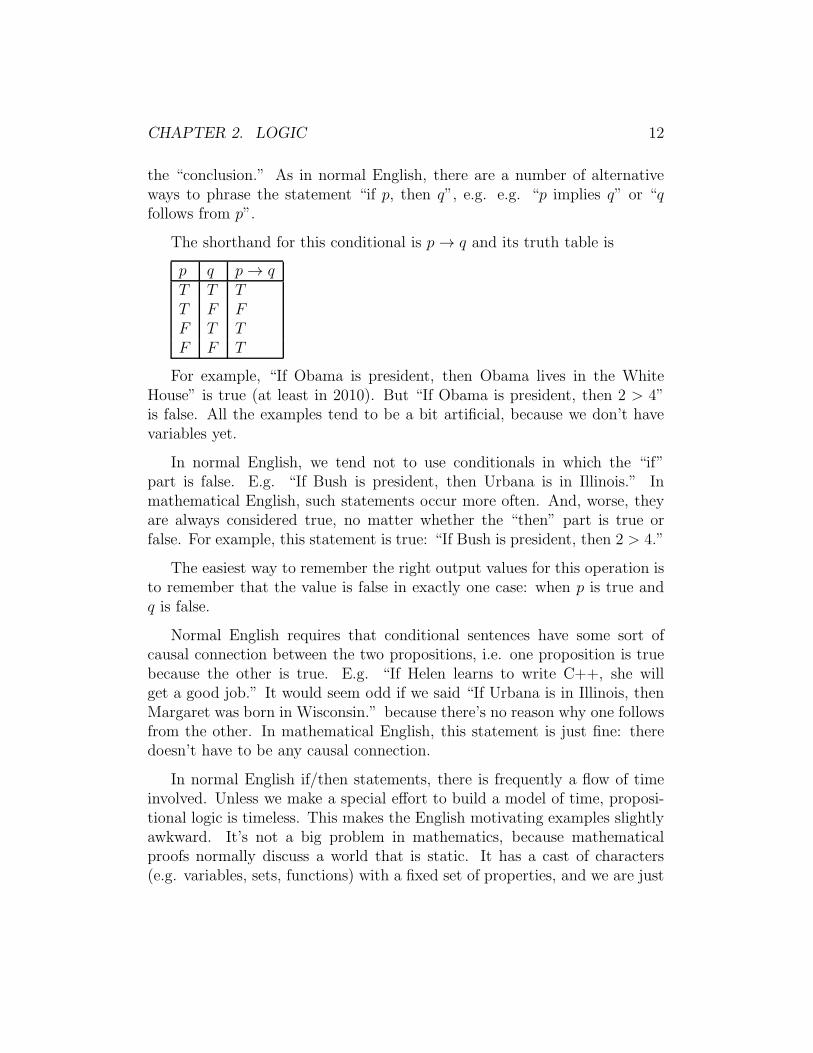
CHAPTER 2. LOGIC 12
the “conclusion.” As in normal English, there are a number of alternativeways to phrase the statement “if p, then q”, e.g. e.g. “p implies q” or “qfollows from p”.
The shorthand for this conditional is p → q and its truth table is
p q p → qT T TT F FF T TF F T
For example, “If Obama is president, then Obama lives in the WhiteHouse” is true (at least in 2010). But “If Obama is president, then 2 > 4”is false. All the examples tend to be a bit artificial, because we don’t havevariables yet.
In normal English, we tend not to use conditionals in which the “if”part is false. E.g. “If Bush is president, then Urbana is in Illinois.” Inmathematical English, such statements occur more often. And, worse, theyare always considered true, no matter whether the “then” part is true orfalse. For example, this statement is true: “If Bush is president, then 2 > 4.”
The easiest way to remember the right output values for this operation isto remember that the value is false in exactly one case: when p is true andq is false.
Normal English requires that conditional sentences have some sort ofcausal connection between the two propositions, i.e. one proposition is truebecause the other is true. E.g. “If Helen learns to write C++, she willget a good job.” It would seem odd if we said “If Urbana is in Illinois, thenMargaret was born in Wisconsin.” because there’s no reason why one followsfrom the other. In mathematical English, this statement is just fine: theredoesn’t have to be any causal connection.
In normal English if/then statements, there is frequently a flow of timeinvolved. Unless we make a special effort to build a model of time, proposi-tional logic is timeless. This makes the English motivating examples slightlyawkward. It’s not a big problem in mathematics, because mathematicalproofs normally discuss a world that is static. It has a cast of characters(e.g. variables, sets, functions) with a fixed set of properties, and we are just
CHAPTER 2. LOGIC 13
reasoning about what those properties are. Only very occasionally do wetalk about taking an object and modifying it.
In computer programming, we often see things that look like conditionalstatements, e.g. “if x > 0, then increment y”. But these are commands forthe computer to do something, changing its little world. whereas the similar-looking mathematical statements are timeless. Formalizing what it meansfor a computer program to “do what it’s supposed to” requires modellinghow the world changes over time. You’ll see this in later CS classes.
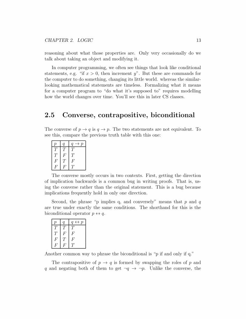
2.5 Converse, contrapositive, biconditional
The converse of p → q is q → p. The two statements are not equivalent. Tosee this, compare the previous truth table with this one:
p q q → pT T TT F TF T FF F T
The converse mostly occurs in two contexts. First, getting the directionof implication backwards is a common bug in writing proofs. That is, us-ing the converse rather than the original statement. This is a bug becauseimplications frequently hold in only one direction.
Second, the phrase “p implies q, and conversely” means that p and qare true under exactly the same conditions. The shorthand for this is thebiconditional operator p ↔ q.
p q q ↔ pT T TT F FF T FF F T
Another common way to phrase the biconditional is “p if and only if q.”
The contrapositive of p → q is formed by swapping the roles of p andq and negating both of them to get ¬q → ¬p. Unlike the converse, the

CHAPTER 2. LOGIC 14
contrapositive is equivalent to the original statement. Here’s a truth tableshowing why:
p q ¬q ¬p ¬q → ¬pT T F F TT F T F FF T F T TF F T T T
To figure out the last column of the table, recall that ¬q → ¬p will befalse in only one case: when the hypothesis (¬q) is true and the conclusion(¬p) is false.
Let’s consider what these variations look like in an English example:
• If it’s below zero, my car won’t start.
• converse: If my car won’t start, it’s below zero
• contrapositive: If my car will start, then it’s not below zero.
2.6 Complex statements
Very complex statements can be made using combinations of connectives.E.g. “If it’s below zero or my car does not have gas, then my car won’t startand I can’t go get groceries.” This example has the form
(p ∨ ¬q) → (¬r ∧ ¬s)
The shorthand notation is particularly useful for manipulating complicatedstatements, e.g. figuring out the negative of a statement.
When you try to read a complex set of propositions all glued togetherwith connectives, there is sometimes a question about which parts to grouptogether first. English is a bit vague about the rules. So, for example, inthe previous example, you need to use common sense to figure out that “Ican’t go get groceries” is intended to be part of the conclusion of the if/thenstatement.
CHAPTER 2. LOGIC 15
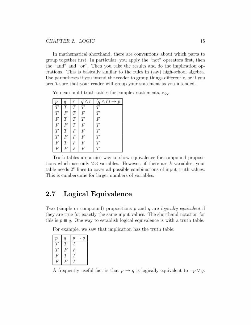
In mathematical shorthand, there are conventions about which parts togroup together first. In particular, you apply the “not” operators first, thenthe “and” and “or”. Then you take the results and do the implication op-erations. This is basically similar to the rules in (say) high-school algebra.Use parentheses if you intend the reader to group things differently, or if youaren’t sure that your reader will group your statement as you intended.
You can build truth tables for complex statements, e.g.
p q r q ∧ r (q ∧ r) → pT T T T TT F T F TF T T T FF F T F TT T F F TT F F F TF T F F TF F F F T
Truth tables are a nice way to show equivalence for compound proposi-tions which use only 2-3 variables. However, if there are k variables, yourtable needs 2k lines to cover all possible combinations of input truth values.This is cumbersome for larger numbers of variables.
2.7 Logical Equivalence
Two (simple or compound) propositions p and q are logically equivalent ifthey are true for exactly the same input values. The shorthand notation forthis is p ≡ q. One way to establish logical equivalence is with a truth table.
For example, we saw that implication has the truth table:
p q p → qT T TT F FF T TF F T
A frequently useful fact is that p → q is logically equivalent to ¬p ∨ q.
CHAPTER 2. LOGIC 16
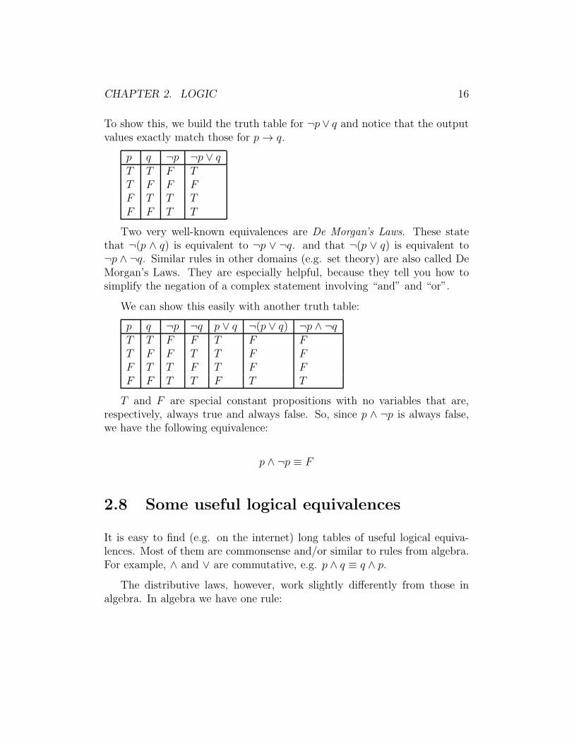
To show this, we build the truth table for ¬p ∨ q and notice that the outputvalues exactly match those for p → q.
p q ¬p ¬p ∨ qT T F TT F F FF T T TF F T T
Two very well-known equivalences are De Morgan’s Laws. These statethat ¬(p ∧ q) is equivalent to ¬p ∨ ¬q. and that ¬(p ∨ q) is equivalent to¬p ∧ ¬q. Similar rules in other domains (e.g. set theory) are also called DeMorgan’s Laws. They are especially helpful, because they tell you how tosimplify the negation of a complex statement involving “and” and “or”.
We can show this easily with another truth table:
p q ¬p ¬q p ∨ q ¬(p ∨ q) ¬p ∧ ¬qT T F F T F FT F F T T F FF T T F T F FF F T T F T T
T and F are special constant propositions with no variables that are,respectively, always true and always false. So, since p ∧ ¬p is always false,we have the following equivalence:
p ∧ ¬p ≡ F
2.8 Some useful logical equivalences
It is easy to find (e.g. on the internet) long tables of useful logical equiva-lences. Most of them are commonsense and/or similar to rules from algebra.For example, ∧ and ∨ are commutative, e.g. p ∧ q ≡ q ∧ p.
The distributive laws, however, work slightly differently from those inalgebra. In algebra we have one rule:

CHAPTER 2. LOGIC 17
a(b+ c) = ab+ ac
where as in logic we have two rules:
p ∨ (q ∧ r) ≡ (p ∨ q) ∧ (p ∨ r)
p ∧ (q ∨ r) ≡ (p ∧ q) ∨ (p ∧ r)
So, in logic, you can distribute either operator over the other. Also,arithmetic has a clear rule that multiplication is done first, so the righthandside doesn’t require parentheses. The order of operations is less clear for thelogic, so more parentheses are required.
2.9 Negating propositions
An important use of logical equivalences is to help you correctly state thenegation of a complex proposition, i.e. what it means for the complex propo-sition not to be true. This is important when you are trying to prove a claimfalse or convert a statement to its contrapositive. Also, looking at the nega-tion of a definition or claim is often helpful for understanding precisely whatthe definition or claim means. Having clear mechanical rules for negation isimportant when working with concepts that are new to you, when you haveonly limited intuitions about what is correct.
For example, suppose we have a claim like “If M is regular, then M isparacompact or M is not Lindelof.” I’m sure you have no idea whether thisis even true, because it comes from a math class you are almost certain notto have taken. However, you can figure out its negation.
First, let’s convert the claim into shorthand so we can see its structure.Let r be “M is regular”, p be “M is paracompact”, and l be “M is Lindelof.”Then the claim would be r → (p ∨ ¬l).
The negation of r → (p∨¬l) is ¬(r → (p∨¬l)). However, to do anythinguseful with this negated expression, we normally need to manipulate it into anequivalent expression that has the negations on the individual propositions.
The key equivalences used in doing this manipulation are:

CHAPTER 2. LOGIC 18
• ¬(¬p) ≡ p
• ¬(p ∧ q) ≡ ¬p ∨ ¬q
• ¬(p ∨ q) ≡ ¬p ∧ ¬q
• ¬(p → q) ≡ p ∧ ¬q.
The last of these follows from an equivalence we saw above: p → q ≡ ¬p∨qplus one of DeMorgan’s laws.
So we have
¬(r → (p ∨ ¬l)) ≡ r ∧ ¬(p ∨ ¬l) ≡ r ∧ ¬p ∧ ¬¬l ≡ r ∧ ¬p ∧ l
So the negation of our original claim is “M is regular and M is notparacompact and M is Lindelof.” Knowing the mechanical rules helps youhandle situations where your logical intuitions aren’t fully up to the task ofjust seeing instinctively what the negation should look like. Mechanical rulesare also very helpful when you are tired or stressed (e.g. during an exam).
Notice that we’ve also derived a new logical equivalence ¬(r → (p∨¬l)) ≡r ∧ ¬p ∧ l by applying a sequence of known equivalences. This is how weestablish new equivalences when truth tables get unwieldy.
2.10 Predicates and Variables
Propositions are a helpful beginning but too rigid to represent most of theinteresting bits of mathematics. To do this, we need predicate logic, whichallows variables and predicates that take variables as input. We’ll get startedwith predicate logic now, but delay covering some of the details until theybecome relevant to the proofs we’re looking at.
A predicate is a statement that becomes true or false if you substitutein values for its variables. For example, “x2 ≥ 10” or “y is winter hardy.”

CHAPTER 2. LOGIC 19
Suppose we call these P (x) and Q(y). Then Q(y) is true if y is “mint” butnot if y is “tomato”.1
If we substitute concrete values for all the variables in a predicate, we’reback to having a proposition. That wasn’t much use, was it?
The main use of predicates is to make general statements about whathappens when you substitute a variety of values for the variables. For exam-ple:
P(x) is true for every x
For example, “For every integer x, x2 ≥ 10” (false).
Consider “For all x, 2x ≥ x.” Is this true or false? This depends on whatvalues x can have. Is x any integer? In that case the claim is false. But if xis supposed to be a natural number, then the claim is true.
In order to decide whether a statement involving quantifiers is true, youneed to know what types of values are allowed for each variable. Good stylerequires that you state the type of the variable explicitly when you introduceit, e.g. “For all natural numbers x, 2x ≥ x.” Exceptions involve caseswhere the type is very, very clear from the context, e.g. when a whole longdiscussion is all about (say) the integers. If you aren’t sure, a redundant typestatement is a minor problem whereas a missing type statement is sometimesa big problem.
2.11 Other quantifiers
The general idea of a quantifier is that it expresses express how many ofthe values in the domain make the claim true. Normal English has a widerange of quantifiers which tell you roughly how many of the values work, e.g.“some”, “a couple”, “a few”, “many”, “most.” For example, “most studentsin this class have taken a programming class.”
1A winter hardy plant is a plant that can survive the winter in a cold climate, e.g. here
in central Illinois.

CHAPTER 2. LOGIC 20
By contrast, mathematics uses only three quantifiers, one of which is usedrarely. We’ve seen the universal quantifier “for all.” The other common oneis the existential quantifier “there exists,” as in
There is an integer x such that x2 = 0.
In normal English, when we say that there is an object with some prop-erties, this tends to imply that there’s only one or perhaps only a couple. Ifthere were many objects with this property, we normally expect the speakerto say so. So it would seem odd to say
There is an integer x such that x2 > 0.
Or
There exists an integer x such that 5 < x < 100.
Mathematicians, however, are happy to say things like that. When theysay “there exists an x,” with certain properties, they mean that there existsat least one x with those properties. They are making no claims about howmany such x’s there are.
However, it is sometimes important to point out when one and only one xhas some set of properties. The mathematical jargon for this uses the uniqueexistence quantifier, as in:
There is a unique integer x such that x2 = 0.
Mathematicians use the adjective “unique” to mean that there’s only onesuch object (similar to the normal usage but not quite the same).
2.12 Notation
The universal quantifier has the shorthand notation ∀. For example,

CHAPTER 2. LOGIC 21
∀x ∈ R, x2 + 3 ≥ 0
In this sentence, ∀ is the quantifier. x ∈ R declares the variable and the set(R) from which its values can be taken, called its domain or its replacementset. As computer scientists, we can also think of this as declaring the typeof x, just as in a computer program. Finally, x2 + 3 ≥ 0 is the predicate.
The existential quantifier is written ∃, e.g. ∃y ∈ R, y =√2. Notice that
we don’t write “such that” when the quantifier is in shorthand. The uniqueexistence quantifier is written ∃! as in ∃!x ∈ R, x2 = 0. When existentialquantifiers are written in English, rather than shorthand, we need to add thephrase “such that” to make the English sound right, e.g.
There exists a real number y such that y =√2.
There’s no deep reason for adding “such that.” It’s just a quirk about howmathematical English is written, which you should copy so that your writtenmathematics looks professional. “Such that” is sometimes abbreviated “s.t.”
2.13 Useful notation
If you want to state a claim about two numbers, you can use two quantifiersas in:
∀x ∈ R, ∀y ∈ R, x+ y ≥ x
This is usually abbreviated to
∀x, y ∈ R, x+ y ≥ x
This means “for all real numbers x and y, x+ y ≥ x” (which isn’t true).
In such a claim, the two variables x and y might contain different values,but it’s important to realize that they might also be equal. For example, thefollowing sentence is true:

CHAPTER 2. LOGIC 22
∃x, y ∈ Z, x− y = 0
We saw above that the statement “if p, then q” has the contrapositive“if ¬q, then ¬p.” This transformation can be extended to statements with aquantifier (typically universal). For example, the statement
∀x, if p(x), then q(x)
would have a contrapositive
∀x, if ¬q(x), then ¬p(x)
Notice that the quantifier stays the same: we only transform the if/thenstatement inside it.
2.14 Notation for 2D points
When writing mathematics that involves 2D points and quantifiers, you haveseveral notational options. You can write something like ∀x, y ∈ Z (“for anyintegers x and y”) and then later refer to the pair (x, y). Or you can treatthe pair (x, y) as a single variable, whose replacement set is all 2D points.For example, the following says that the real plane (R2) contains a point onthe unit circle:
∃(x, y) ∈ R2, x2 + y2 = 1
Another approach is to write something like
∃p ∈ R2, p is on the unit circle
When you later need to make precise what it means to be “on the unit circle,”you will have to break up p into its two coordinates. At that point, you saythat that since p is a point on the plane, it must have the form (x, y), wherex and y are real numbers. This defines the component variables you need toexpand the definition of “on the unit circle” into the equation x2 + y2 = 1.
CHAPTER 2. LOGIC 23
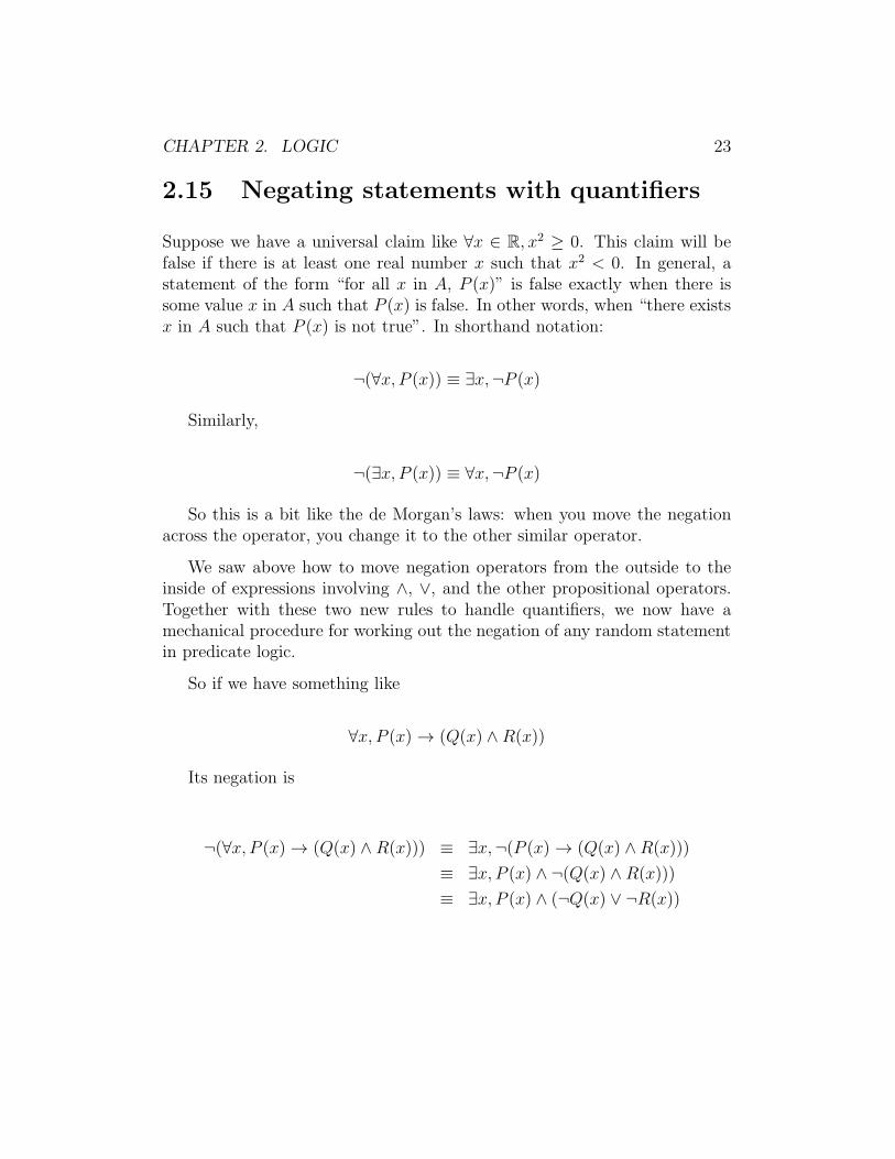
2.15 Negating statements with quantifiers
Suppose we have a universal claim like ∀x ∈ R, x2 ≥ 0. This claim will befalse if there is at least one real number x such that x2 < 0. In general, astatement of the form “for all x in A, P (x)” is false exactly when there issome value x in A such that P (x) is false. In other words, when “there existsx in A such that P (x) is not true”. In shorthand notation:
¬(∀x, P (x)) ≡ ∃x,¬P (x)
Similarly,
¬(∃x, P (x)) ≡ ∀x,¬P (x)
So this is a bit like the de Morgan’s laws: when you move the negationacross the operator, you change it to the other similar operator.
We saw above how to move negation operators from the outside to theinside of expressions involving ∧, ∨, and the other propositional operators.Together with these two new rules to handle quantifiers, we now have amechanical procedure for working out the negation of any random statementin predicate logic.
So if we have something like
∀x, P (x) → (Q(x) ∧ R(x))
Its negation is
¬(∀x, P (x) → (Q(x) ∧ R(x))) ≡ ∃x,¬(P (x) → (Q(x) ∧R(x)))
≡ ∃x, P (x) ∧ ¬(Q(x) ∧ R(x)))
≡ ∃x, P (x) ∧ (¬Q(x) ∨ ¬R(x))
CHAPTER 2. LOGIC 24
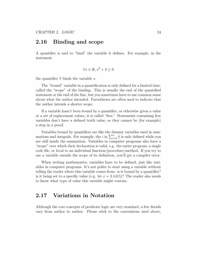
2.16 Binding and scope
A quantifier is said to “bind” the variable it defines. For example, in thestatement
∀x ∈ R, x2 + 3 ≥ 0
the quantifier ∀ binds the variable x.
The “bound” variable in a quantification is only defined for a limited time,called the “scope” of the binding. This is usually the end of the quantifiedstatement or the end of the line, but you sometimes have to use common senseabout what the author intended. Parentheses are often used to indicate thatthe author intends a shorter scope.
If a variable hasn’t been bound by a quantifier, or otherwise given a valueor a set of replacement values, it is called “free.” Statements containing freevariables don’t have a defined truth value, so they cannot be (for example)a step in a proof.
Variables bound by quantifiers are like the dummy variables used in sum-mations and integrals. For example, the i in
∑n
i=01iis only defined while you
are still inside the summation. Variables in computer programs also have a“scope” over which their declaration is valid, e.g. the entire program, a singlecode file, or local to an individual function/procedure/method. If you try touse a variable outside the scope of its definition, you’ll get a compiler error.
When writing mathematics, variables have to be defined, just like vari-ables in computer programs. It’s not polite to start using a variable withouttelling the reader where this variable comes from: is it bound by a quantifier?is it being set to a specific value (e.g. let x = 3.1415)? The reader also needsto know what type of value this variable might contain.
2.17 Variations in Notation
Although the core concepts of predicate logic are very standard, a few detailsvary from author to author. Please stick to the conventions used above,

CHAPTER 2. LOGIC 25
because it’s less confusing if we all use the same notation. However, don’tbe surprised if another class or book does things differently. For example:
• There are several conventions about inserting commas after the quan-tifier and/or parentheses around the following predicate. We won’t bepicky about this.
• Some subfields (but not this class) have a convention that “and” isapplied before “or,” so that parentheses around “and” operations canbe omitted. We’ll keep the parentheses in such cases.
• Some authors use certain variations of “or” (e.g. “either ... or”) with anexclusive meaning, when writing mathematical English. In this class,always read “or” as inclusive unless there is an explicit reason to dootherwise (e.g. “X and Y, but not both”).
• In circuits and certain programming languages, “true” and “false” arerepresented by 1 and 0. There are also many different shorthand nota-tions for connectives such as “and”.
Chapter 3
Proofs
Many mathematical proofs use a small range of standard outlines: directproof, examples/counter-examples, and proof by contradiction and contra-positive. These notes explain these basic proof methods, as well as how touse definitions of new concepts in proofs. More advanced methods (e.g. proofby induction) will be covered later.
3.1 Proving a universal statement
Now, let’s consider how to prove a claim like
For every rational number q, 2q is rational.
First, we need to define what we mean by “rational”.
A real number r is rational if there are integers m and n, n 6= 0, suchthat r = m
n.
In this definition, notice that the fraction mn
does not need to satisfyconditions like being proper or in lowest terms So, for example, zero is rationalbecause it can be written as 0
1. Howevet, it’s critical that the two numbers
26
CHAPTER 3. PROOFS 27
in the fraction be integers, since even irrational numbers can be written asfractions with non-integers on the top and/or bottom. E.g. π = π
1.
The simplest technique for proving a claim of the form ∀x ∈ A, P (x) isto pick some representative value for x.1. Think about sticking your handinto the set A with your eyes closed and pulling out some random element.You use the fact that x is an element of A to show that P (x) is true. Here’swhat it looks like for our example:
Proof: Let q be any rational number. From the definition of“rational,” we know that q = m
nwhere m and n are integers and
n is not zero. So 2q = 2mn
= 2mn. Since m is an integer, so is
2m. So 2q is also the ratio of two integers and, therefore, 2q isrational.
At the start of the proof, notice that we expanded the word “rational”into what its definition said. At the end of the proof, we went the otherway: noticed that something had the form required by the definition andthen asserted that it must be a rational.
WARNING!! Abuse of notation. Notice that the above definition of“rational” used the word “if”. If you take this literally, it would mean that thedefinition could be applied only in one direction. This isn’t what’s meant.Definitions are always intended to work in both directions. Technically, Ishould have written “if and only if” (frequently shortened to “iff”). Thislittle misuse of “if” in definitions is very, very common.
Notice also that we spelled out the definition of “rational” but we justfreely used facts from high school algebra as if they were obvious. In general,when writing proofs, you and your reader come to some agreement aboutwhat parts of math will be considered familiar and obvious, and which re-quire explicit discussion. In practical terms, this means that, when writingsolutions to homework problems, you should try to mimic the level of detail inexamples presented in lecture and in model solutions to previous homeworks.
1The formal name for this is “universal instantiation.”

CHAPTER 3. PROOFS 28
3.2 Another example of direct proof involv-
ing odd and even
Here’s another claim that can be proved by direct proof.
Claim 1 For any integer k, if k is odd then k2 is odd.
This has a slightly different form from the previous claim: ∀x ∈ Z, if P (x),then Q(x)
Before doing the actual proof, we first need to be precise about what wemean by “odd”. And, while we are on the topic, what we mean by “even.”
Definition 1 An integer n is even if there is an integer m such that n = 2m.
Definition 2 An integer n is odd if there is an integer m such that n =2m+ 1.
Such definitions are sometimes written using the jargon “has the form,” asin “An integer n is even if it has the form 2m, where m is an integer.”
We’ll assume that it’s obvious (from our high school algebra) that everyinteger is even or odd, and that no integer is both even and odd. You prob-ably also feel confident that you know which numbers are odd or even. Anexception might be zero: notice that the above definition makes it definitelyeven. This is the standard convention in math and computer science.
Using these definitions, we can prove our claim as follows:
Proof of Claim 1: Let k be any integer and suppose that k is odd.We need to show that k2 is odd.
Since k is odd, there is an integer j such that k = 2j + 1. Thenwe have
k2 = (2j + 1)2 = 4j2 + 4j + 1 = 2(2j2 + 2j) + 1
Since j is an integer, 2j2 + 2j is also an integer. Let’s call it p.Then k2 = 2p+ 1. So, by the definition of odd, k2 is odd.

CHAPTER 3. PROOFS 29
As in the previous proof, we used our key definition twice in the proof:once at the start to expand a technical term (“odd”) into its meaning, thenagain at the end to summarize our findings into the appropriate technicalterms.
At the start of the proof, notice that we chose a random (or “arbitrary”in math jargon) integer k, like last time. However, we also “supposed” thatthe hypothesis of the if/then statement was true. It’s helpful to collect upall your given information right at the start of the proof, so you know whatyou have to work with.
The comment about what we need to show is not necessary to the proof.It’s sometimes included because it’s helpful to the reader. You may also wantto include it because it’s helpful to you to remind you of where you need toget to at the end of the proof.
Similarly, introducing the variable p isn’t really necessary with a claimthis simple. However, using new variables to create an exact match to adefinition may help you keep yourself organized.
3.3 Direct proof outline
In both of these proofs, we started from the known information (anythingin the variable declarations and the hypothesis of the if/then statement)and moved gradually towards the information that needed to be proved (theconclusion of the if/then statement). This is the standard “logical” order fora direct proof. It’s the easiest order for a reader to understand.
When working out your proof, you may sometimes need to reason back-wards from your desired conclusion on your scratch paper. However, whenyou write out the final version, reorder everything so it’s in logical order.
You will sometimes see proofs that are written partly in backwards order.This is harder to do well and requires a lot more words of explanation to helpthe reader follow what the proof is trying to do. When you are first startingout, especially if you don’t like writing a lot of comments, it’s better to stickto a straightforward logical order.
CHAPTER 3. PROOFS 30
3.4 Proving existential statements
Here’s an existential claim:
Claim 2 There is an integer k such that k2 = 0.
An existential claim such as the following asserts the existence of an objectwith some set of properties. So it’s enough to exhibit some specific concreteobject, of our choosing, with the required properties. So our proof can bevery simple:
Proof: Zero is such an integer. So the statement is true.
We could spell out a bit more detail, but it’s really not necessary. Proofsof existential claims are often very short, though there are exceptions.
Notice one difference from our previous proofs. When we pick a value toinstantiate a universally quantified variable, we have no control over exactlywhat the value is. We have to base our reasoning just on what set it belongsto. But when we are proving an existential claim, we get to pick our ownfavorite choice of concrete value, in this case zero.
Don’t prove an existential claim using a general argument about whythere must exist numbers with these properties.2 This is not only overkill,but very hard to do correctly and harder on the reader. Use a specific,concrete example.
3.5 Disproving a universal statement
Here’s a universal claim that is false:
Claim 3 Every rational number q has a multiplicative inverse.
2In higher mathematics, you occuasionally must make an abstract argument about
existence because it’s not feasible to produce a concrete example. We will see one example
towards the end of this course. But this is very rare.
CHAPTER 3. PROOFS 31
Definition 3 If q and r are real numbers, r is a multiplicative inverse for qif qr = 1.
In general, a statement of the form “for all x in A, P (x)” is false exactlywhen there is some value y in A for which P (y) is false.3 So, to disprove auniversal claim, we need to prove an existential statement. So it’s enough toexhibit one concrete value (a “counter-example”) for which the claim fails.In this case, our disproof is very simple:
Disproof of Claim 3: This claim isn’t true, because we know fromhigh school algebra that zero has no inverse.
Don’t try to construct a general argument when a single specific coun-terexample would be sufficient.
3.6 Disproving an existential statement
There’s a general pattern here: the negation of ∀x, P (x) is ∃x,¬P (x). So thenegation of a universal claim is an existential claim. Similarly the negation of∃x, P (x) is ∀x,¬P (x). So the negation of an existential claim is a universalone.
Suppose we want to disprove an existential claim like:
Claim 4 There is an integer k such that k2 + 2k + 1 < 0.
We need to make a general argument that, no matter what value of k wepick, the equation won’t hold. So we need to prove the claim
Claim 5 For every integer k, it’s not the case that k2 + 2k + 1 < 0.
Or, said another way,
3Notice that “for which” is occasionally used as a variant of “such that.” In this case,
it makes the English sound very slightly better.

CHAPTER 3. PROOFS 32
Claim 6 For every integer k, k2 + 2k + 1 ≥ 0.
The proof of this is fairly easy:
Proof: Let k be an integer. Then (k+1)2 ≥ 0 because the squareof any real number is non-negative. But (k+1) = k2+2k+1. So,by combining these two equations, we find that k2 + 2k + 1 ≥ 0.
3.7 Recap of proof methods
So, our general pattern for selecting the proof type is:
prove disproveuniversal general argument specific counter-exampleexistential specific example general argument
Both types of proof start off by picking an element x from the domainof the quantification. However, for the general arguments, x is a randomelement whose identity you don’t know. For the proofs requiring specificexamples, you can pick x to be your favorite specific concrete value.
3.8 Direct proof: example with two variables
Let’s do another example of direct proof. First, let’s define
Definition 4 An integer n is a perfect square if n = k2 for some integer k.
And now consider the claim:
Claim 7 For any integers m and n, if m and n are perfect squares, then sois mn.
Proof: Let m and n be integers and suppose that m and n areperfect squares.
CHAPTER 3. PROOFS 33
By the definition of “perfect square”, we know that m = k2 andn = j2, for some integers k and j. So then mn is k2j2, which isequal to (kj)2. Since k and j are integers, so is kj. Since mnis the square of the integer kj, mn is a perfect square, which iswhat we needed to show.
Notice that we used a different variable name in the two uses of thedefinition of perfect square: k the first time and j the second time. It’simportant to use a fresh variable name each time you expand a definitionlike this. Otherwise, you could end up forcing two variables (m and n in thiscase) to be equal when that isn’t (or might not be) true.
Notice that the phrase “which is what we needed to show” helps tell thereader that we’re done with the proof. It’s polite to indicate the end inone way or another. In typed notes, it may be clear from the indentation.Sometimes, especially in handwritten proofs, we put a box or triangle of dotsor Q.E.D. at the end. Q.E.D. is short for Latin “Quod erat demonstrandum,”which is just a translation of “what we needed to show.”
3.9 Another example with two variables
Here’s another example of a claim involving two variables:
Claim 8 For all integers j and k, if j and k are odd, then jk is odd.
A direct proof would look like:
Proof: Let j and k be integers and suppose they are both odd.Because j is odd, there is an integer p such that j = 2p + 1.Similarly, there is an integer q such that k = 2q + 1.
So then jk = (2p+1)(2q+1) = 4pq+2p+2q+1 = 2(2pq+p+q)+1.Since p and q are both integers, so is 2pq + p + q. Let’s call itm. Then jk = 2m+ 1 and therefore jk is odd, which is what weneeded to show.

CHAPTER 3. PROOFS 34
3.10 Proof by cases
When constructing a proof, sometimes you’ll find that part of your giveninformation has the form “p or q.” Perhaps your claim was stated using“or,” or perhaps you had an equation like |x| > 6 which translates into anor (x > 6 or x < −6) when you try to manipulate it. When the giveninformation allows two or more separate possibilities, it is often best to usea technique called “proof by cases.”
In proof by cases, you do part of the proof two or more times, once foreach of the possibilities in the “or.” For example, suppose that our claim is:
Claim 9 For all integers j and k, if j is even or k is even, then jk is even.
We can prove this as follows:
Proof: Let j and k be integers and suppose that j is even or k iseven. There are two cases:
Case 1: j is even. Then j = 2m, where m is an integer. So thejk = (2m)k = 2(mk). Since m and k are integers, so is mk. Sojk must be even.
Case 2: k is even. Then k = 2n, where n is an integer. So thejk = j(2n) = 2(nj). Since n and j are integers, so is nj. So jkmust be even.
So jk is even in both cases, which is what we needed to show.
It is ok to have more than two cases. It’s also ok if the cases overlap,e.g. one case might assume that x ≤ 0 and another case might assume thatx ≥ 0. However, you must be sure that all your cases, taken together, coverall the possibilities.
In this example, each case involved expanding the definition of “even.”We expanded the definition twice but, unlike our earlier examples, only oneexpansion is active at a given time. So we could have re-used the variable mwhen we expanded “even” in Case 2. I chose to use a fresh variable name(n) because this is a safer strategy if you aren’t absolutely sure when re-useis ok.
CHAPTER 3. PROOFS 35
3.11 Rephrasing claims
Sometimes you’ll be asked to prove a claim that’s not in a good form for adirect proof. For example:
Claim 10 There is no integer k such that k is odd and k2 is even.
It’s not clear how to start a proof for a claim like this. What is our giveninformation and what do we need to show?
In such cases, it is often useful to rephrase your claim using logical equiv-alences. For example, the above claim is equivalent to
Claim 11 For every integer k, it is not the case that k is odd and k2 is even.
By DeMorgan’s laws, this is equivalent to
Claim 12 For every integer k, k is not odd or k2 is not even.
Since we’re assuming we all know that even and odd are opposites, thisis the same as
Claim 13 For every integer k, k is not odd or k2 is odd.
And we can restate this as an implication using the fact that ¬p ∨ q isequivalent to p → q:
Claim 14 For every integer k, if k is odd then k2 is odd.
Our claim is now in a convenient form: a universal if/then statementwhose hypothesis contains positive (not negated) facts. And, in fact, weproved this claim earlier in these notes.

CHAPTER 3. PROOFS 36
3.12 Proof by contrapositive
A particularly common sort of rephrasing is to replace a claim by its contra-positive. If the original claim was ∀x, P (x) → Q(x) then its contrapositiveis ∀x,¬Q(x) → ¬P (x). Remember that any if/then statement is logicallyequivalent to its contrapositive.
Remember that contructing the hypothesis requires swapping the hypoth-esis with the conclusion AND negating both of them. If you do only half ofthis transformation, you get a statement that isn’t equivalent to the original.For example, the converse ∀x,Q(x) → P (x) is not equivalent to the originalclaim.
For example, suppose that we want to prove
Claim 15 For any integers a and b, if a + b ≥ 15, then a ≥ 8 or b ≥ 8.
This is hard to prove in its original form, because we’re trying to useinformation about a derived quantity to prove something about more basicquantities. If we rephrase as the contrapositive, we get
Claim 16 For any integers a and b, if it’s not the case that a ≥ 8 or b ≥ 8,then it’s not the case that a+ b ≥ 15.
And this is equivalent to:
Claim 17 For any integers a and b, if a < 8 and b < 8, then a+ b < 15.
Notice that when we negated the conclusion of the original statement, weneeded to change the “or” into an “and” (DeMorgan’s Law).
When you do this kind of rephrasing, your proof should start by explain-ing to the reader how you rephrased the claim. It’s technically enough to saythat you’re proving the contrapositive. But, for a beginning proof writer, it’sbetter to actually write out the contrapositive of the claim. This gives you achance to make sure you have constructed the contrapositive correctly. And,while you are writing the rest of the proof, it helps remind you of exactlywhat is given and what you need to show.
So a proof our our original claim might look like:

CHAPTER 3. PROOFS 37
Proof: We’ll prove the contrapositive of this statement. That is,for any integers a and b, if a < 8 and b < 8, then a + b < 15.
So, suppose that a and b are integers such that a < 8 and b < 8.Since they are integers (not e.g. real numbers), this implies thata ≤ 7 and b ≤ 7. Adding these two equations together, we findthat a+ b ≤ 14. But this implies that a+ b < 15. �
There is no hard-and-fast rule about when to switch to the contrapositiveof a claim. If you are stuck trying to write a direct proof, write out thecontrapositive of the claim and see whether that version seems easier toprove.
3.13 Another example of proof by contrapos-
itive
Here’s another example where it works well to convert to the contrapositive:
Claim 18 For any integer k, if 3k + 1 is even, then k is odd.
If we rephrase as the contrapositive, we get:
Claim 19 For any integer k, if k is even, 3k + 1 is odd.
So our complete proof would look like:
Proof: We will prove the contrapositive of this claim, i.e. thatfor any integer k, if k is even, 3k + 1 is odd.
So, suppose that k is an integer and k is even. Then, k = 2m forsome integer m. Then 3k+ 1 = 3(2m) + 1 = 2(3m) + 1. Since mis an integer, so is 3m. So 3k+ 1 must be odd, which is what weneeded to show.
CHAPTER 3. PROOFS 38
3.14 Proof by contradiction
Another way to prove a claim P is to show that its negation ¬P leads to acontradiction. If ¬P leads to a contradiction, then ¬P can’t be true, andtherefore P must be true. A contradiction can be any statement that is well-known to be false or a set of statements that are obviously inconsistent withone another, e.g. n is odd and n is even, or x < 2 and x > 7.
Proof by contradiction is typically used to prove claims that a certaintype of object cannot exist. The negation of the claim then says that anobject of this sort does exist. For example:
Claim 20 There is no largest even integer.
Proof: Suppose not. That is, suppose that there were a largesteven integer. Let’s call it k.
Since k is even, it has the form 2n, where n is an integer. Considerk + 2. k + 2 = (2n) + 2 = 2(n + 1). So k + 2 is even. But k + 2is larger than k. This contradicts our assumption that k was thelargest even integer. So our original claim must have been true.�
The proof starts by informing the reader that you’re about to use proofby contradiction. The phrase “suppose not” is one traditional way of doingthis. Next, you should spell out exactly what the negation of the claim is.Then use mathematical reasoning (e.g. algebra) to work forwards until youdeduce some type of contradiction.
3.15√2 is irrational
One of the best known examples of proof by contradiction is the proof that√2 is irrational. This proof, and consequently knowledge of the existence of
irrational numbers, apparently dates back to the Greek philosopher Hippasusin the 5th century BC.
CHAPTER 3. PROOFS 39
We defined a rational number to be a real number that can be written asa fraction a
b, where a and b are integers and b is not zero. If a number can
be written as such a fraction, it can be written as a fraction in lowest terms,i.e. where a and b have no common factors. If a and b have common factors,it’s easy to remove them.
Also, we proved (above) that, for any integer k, if k is odd then k2 is odd.So the contrapositive of this statement must also be true: (*) if k2 is eventhen k is even.
Now, we can prove our claim:
Suppose not. That is, suppose that√2 were rational.
Then we can write√2 as a fraction a
bwhere a and b are integers
with no common factors.
Since√2 = a
b, 2 = a2
b2. So 2b2 = a2.
By the definition of even, this means a2 is even. But then a mustbe even, by (*) above. So a = 2n for some integer n.
If a = 2n and 2b2 = a2, then 2b2 = 4n2. So b2 = 2n2. This meansthat b2 is even, so b must be even.
We now have a contradiction. a and b were chosen not to haveany common factors. But they are both even, i.e. they are bothdivisible by 2.
Because assuming that√2 was rational led to a contradiction, it
must be the case that√2 is irrational. �

Chapter 4
Number Theory
We’ve now covered most of the basic techniques for writing proofs. So we’regoing to start applying them to specific topics in mathematics, starting withnumber theory.
Number theory is a branch of mathematics concerned with the behaviorof integers. It has very important applications in cryptography and in thedesign of randomized algorithms. Randomization has become an increasinglyimportant technique for creating very fast algorithms for storing and retriev-ing objects (e.g. hash tables), testing whether two objects are the same (e.g.MP3’s), and the like. Much of the underlying theory depends on facts aboutwhich numbers evenly divide one another and which numbers are prime.
4.1 Factors and multiples
You’ve undoubtedly seen some of the basic ideas (e.g. divisibility) somewhatinformally in earlier math classes. However, you may not be fully clear onwhat happens with special cases, e.g. zero, negative numbers. We also needclear formal definitions in order to write formal proofs. So, let’s start with
Definition: Suppose that a and b are integers. Then a divides bif b = an for some integer n. a is called a factor or divisor of b. bis called a multiple of a.
40

CHAPTER 4. NUMBER THEORY 41
The shorthand for a divides b is a | b. Be careful about the order. Thedivisor is on the left and the multiple is on the right.
Some examples:
• 7 | 77
• 77 6 | 7
• 7 | 7 because 7 = 7 · 1
• 7 | 0 because 0 = 7 · 0, zero is divisible by any integer.
• 0 6 | 7 because 0 · n will always give you zero, never 7. Zero is a factorof only one number: zero.
• (−3) | 12 because 12 = 3 · −4
• 3 | (−12) because −12 = 3 · −4
A number p is even exactly when 2 | p. The fact that zero is even is justa special case of the fact that zero is divisible by any integer.
4.2 Direct proof with divisibility
We can prove basic facts about divisibility in much the same way we provedbasic facts about even and odd.
Claim 21 For any integers a,b,and c, if a | b and a | c then a | (b+ c).
Proof: Let a,b,and c and suppose that a | b and a | c.Since a | b, there is an integer k such that b = ak (definition ofdivides). Similarly, since a | c, there is an integer j such thatc = aj. Adding these two equations, we find that (b + c) =ak + aj = a(k + j). Since k and j are integers, so is k + j.Therefore, by the definition of divides, a | (b+ c). �

CHAPTER 4. NUMBER THEORY 42
When we expanded the definition of divides for the second time, we useda fresh variable name. If we had re-used k, then we would have wronglyforced b and c to be equal.
The following two claims can be proved in a similar way:
Claim 22 For any integers a,b,and c, if a | b and b | c then a | c. (Transi-tivity of divides.)
Claim 23 For any integers a,b, and c, if a | b, then a | bc.
You’ve probably seen “transitivity” before in the context of inequalities.E.g. if a < b and b < c, then a < c. We’ll get back to the general notion oftransitivity later in the term.
4.3 Stay in the Set
Students are sometimes tempted to rephrase the definition of a | b as “ bais an
integer.” This is not a good idea because it introduces a non-integer rationalnumber into a problem that only needs to involve integers. Stepping outsidethe set of interest in this way is occasionally useful, but more often it leadsto inelegant and/or buggy solutions. This happens for three reasons:
• The purely integer proofs are typically simpler.
• When constructing math from the ground up, the integers are typicallyconstructed first and the rationals built from them. So using rationalsto prove facts about integers can lead to circular proofs.
• On computers, integer operations yield exact answers but floating pointoperations are only approximate. So implementing an integer calcula-tion using real numbers often introduces errors.
CHAPTER 4. NUMBER THEORY 43
4.4 Prime numbers
We’re all familiar with prime numbers from high school. Firming up thedetails:
Definition: an integer q ≥ 2 is prime if the only positive factorsof q are q and 1. An integer q ≥ 2 is composite if it is not prime.
For example, among the integers no bigger than 20, the primes are 2, 3,5, 7, 11, 13, 17, and 19.
A key fact about prime numbers is
Fundanmental Theorem of Arithmetic: Every integer ≥ 2 can bewritten as the product of one or more prime factors. Except forthe order in which you write the factors, this prime factorizationis unique.
The word “unique” here means that there is only one way to factor eachinteger.
For example, 260 = 2 · 2 · 5 · 13 and 180 = 2 · 2 · 3 · 3 · 5.We won’t prove this theorem right now, because it requires a proof tech-
nique called “induction,” which we haven’t seen yet.
There are quite fast algorithms for testing whether a large integer is prime.However, even once you know a number is composite, algorithms for factoringthe number are all fairly slow. The difficulty of factoring large compositenumbers is the basis for a number of well-known cryptographic algorithms(e.g. the RSA algorithm).
4.5 There are infinitely many prime numbers
We can now prove a classic result about prime numbers. So classic, in fact,that it goes back to Euclid, who lived around 300 B.C.

CHAPTER 4. NUMBER THEORY 44
Euclid’s Theorem: There are infinitely many prime numbers.
This is a lightly disguised type of non-existence claim. The theoremcould be restated as “there is no largest prime” or “there is no finite list ofall primes.” So this is a good situation for applying proof by contradiction.
Proof: Suppose not. That is, suppose there were only finitelymany prime numbers. Let’s call them p1, p2, up through pn.
Consider Q = p1p2 · · ·pn + 1.
If you divide Q by one of the primes on our list, you get a re-mainder of 1. So Q isn’t divisible by any of the primes p1, p2,up through pn. However, by the Fundamental Theorem of Arith-metic, Q must have a prime factor (which might be either itselfor some smaller number). This contradicts our assumption thatp1, p2,. . . pn was a list of all the prime numbers. �
Notice one subtlety. We’re not claiming that Q must be prime. Rather,we’re making the much weaker claim that Q isn’t divisible by any of the firstn primes. It’s possible that Q might be divisible by another prime largerthan pn.
4.6 GCD and LCM
If c divides both a and b, then c is called a common divisor of a and b. Thelargest such number is the greatest common divisor of a and b. Shorthandfor this is gcd(a, b).
You can find the GCD of two numbers by inspecting their prime factor-izations and extracting the shared factors. For example, 70 = 2 · 5 · 7 and130 = 2 · 5 · 13. So gcd(70, 130) is 2 · 5 = 10.
Similarly, a common multiple of a and b is a number c such that a|c andb|c. The least common multiple (lcm) is the smallest positive number forwhich this is true. The lcm can be computed using the formula:
CHAPTER 4. NUMBER THEORY 45
lcm(a, b) =ab
gcd(a, b)
For example, lcm(70, 130) = 70·13010
= 910.
If two integers a and b share no common factors, then gcd(a, b) = 1. Sucha pair of integers are called relatively prime.
If k is a non-zero integer, then k divides zero. the largest common divisorof k and zero is k. So gcd(k, 0) = gcd(0, k) = k. However, gcd(0, 0) isn’tdefined. All integers are common divisors of 0 and 0, so there is no greatestone.
4.7 The division algorithm
The obvious way to compute the gcd of two integers is to factor both intoprimes and extract the shared factors. This is easy for small integers. How-ever, it quickly becomes very difficult for larger integers, both for humansand computers. Fortunately, there’s a fast method, called the Euclidean al-gorithm. Before presenting this algorithm, we need some background aboutinteger division.
In general, when we divide one integer by another, we get a quotient anda remainder:
Theorem 1 (Division Algorithm) The Division Algorithm: For any in-tegers a and b, where b is positive, there are unique integers q (the quotient)and r (the remainder) such that a = bq + r and 0 ≤ r < b.
For example, if 13 is divided by 4, the quotient is 3 and the remainder is1. Notice that the remainder is required to be non-negative. So -10 dividedby 7 has the remainder 4, because (−10) = 7 · (−2)+4. This is the standardconvention in mathematics. The word “unique” in this theorem simply meansthat only one pair of number q and r satisfy the pair of equations.
Now, notice the following non-obvious fact about the gcd:

CHAPTER 4. NUMBER THEORY 46
Claim 24 For any integers a, b, q and r, where b is positive, if a = bq + r,then gcd(a, b) = gcd(b, r).
Proof: Suppose that n is some integer which divides both a andb. Then n divides bq and so n divides a − bq. (E.g. use variouslemmas about divides from last week.) But a− bq is just r. So ndivides r.
By an almost identical line of reasoning, if n divides both b andr, then n divides a.
So, the set of common divisors of a and b is exactly the same asthe set of common divisors of b and r. But gcd(a, b) and gcd(b, r)are just the largest numbers in these two sets, so if the sets containthe same things, the two gcd’s must be equal.
If r is the remainder when a is divided by b, then a = bq + r, for someinteger q. So we can immediately conclude that:
Corollary: Suppose that a and b are integers and b is positive.Let r be the remainder when a is divided by b. Then gcd(a, b) =gcd(b, r).
The term “corollary” means that this fact is a really easy consequence ofthe preceding claim.
4.8 Euclidean algorithm
We can now give a fast algorithm for computing gcd, which dates back to Eu-clid. Suppose that remainder(a, b) returns the remainder when a is dividedby b. Then we can compute the gcd as follows:
gcd(a,b: positive integers)
x := a
y := b
while (y > 0)

CHAPTER 4. NUMBER THEORY 47
begin
r := remainder(x,y)
x := y
y := r
end
return x
Let’s trace this algorithm on inputs a = 105 and b = 252. Traces shouldsummarize the values of the most important variables.
x y r = remainder(x, y)105 252 105252 105 42105 42 2142 21 021 0
Since x is smaller than y, the first iteration of the loop swaps x and y.After that, each iteration reduces the sizes of a and b, because a mod b issmaller than b. In the last iteration, y has gone to zero, so we output thevalue of x which is 21.
To verify that this algorithm is correct, we need to convince ourselves oftwo things. First, it must halt, because each iteration reduces the magnitudeof y. Second, by our corollary above, the value of gcd(x, y) does not changefrom iteration to iteration. Moreover, gcd(x, 0) is x, for any non-zero integerx. So the final output will be the gcd of the two inputs a and b.
This is a genuinely very nice algorithm. Not only is it fast, but it involvesvery simple calculations that can be done by hand (without a calculator).It’s much easier than factoring both numbers into primes, especially as theindividual prime factors get larger. Most of us can’t quickly see whether alarge number is divisible by, say, 17.
4.9 Pseudocode
Notice that this algorithm is written in pseudocode. Pseudocode is an ab-stracted type of programming language, used to highlight the important

CHAPTER 4. NUMBER THEORY 48
structure of an algorithm and communicate between researchers who maynot use the same programming language. It borrows many control constructs(e.g. the while loop) from imperative languages such as C. But details re-quired only for a mechanical compiler (e.g. type declarations for all variables)are omitted and equations or words are used to hide details that are easy tofigure out.
If you have taken a programming course, pseudocode is typically easy toread. Many small details are not standardized, e.g. is the test for equalitywritten = or ==? However, it’s usually easy for a human (though not acomputer) to figure out what the author must have intended.
A common question is how much detail to use. Try to use about the sameamount as in the examples shown in the notes. And think about how easilyyour pseudocode could be read by a classmate. Actual C or Java code isalmost never acceptable pseudocode, because it is way too detailed.
4.10 A recursive version of gcd
We can also write gcd as a recursive algorithm
procedure gcd(a,b: positive integers)
r := remainder(a,b)
if (r = 0) return b
else return gcd(b,r)
This code is very simple, because this algorithm has a natural recursivestructure. Our corollary allows us to express the gcd of two numbers in termsof the gcd of a smaller pair of numbers. That is to say, it allows us to reducea larger version of the task to a smaller version of the same task.
4.11 Congruence mod k
Many applications of number theory, particularly in computer science, usemodular arithmetic. In modular arithmetic, there are only a finite set of
CHAPTER 4. NUMBER THEORY 49
numbers and addition “wraps around” from the highest number to the lowestone. This is true, for example, for the 12 hours on a standard US clock: 3hours after 11 o’clock is 2 o’clock, not 14 o’clock.
The formal mathematical definitions of modular arithmetic are based onthe notion of congruence. Specifically, two integers are “congruent mod k”if they differ by a multiple of k. Formally:
Definition: If k is any positive integer, two integers a and b arecongruent mod k (written a ≡ b (mod k)) if k | (a− b).
Notice that k | (a− b) if and only if k | (b− a). So it doesn’t matter whichnumber is subtracted from the other.
For example:
• 17 ≡ 5 (mod 12) (Familiar to those of us who’ve had to convert be-tween US 12-hour clocks and European/military 24-hour clocks.)
• 3 ≡ 10 (mod 7)
• 3 ≡ 38 (mod 7) (Since 38− 3 = 35.)
• 38 ≡ 3 (mod 7)
• −3 ≡ 4 (mod 7) (Since (−3) + 7 = 4.)
• −3 6≡ 3 (mod 7)
• −3 ≡ 3 (mod 6)
• −29 ≡ −13 (mod 8) (Since (−13)− (−29) = 16.)
Congruence mod k is a relaxation of our normal rules for equality ofnumbers, in which we agree that certain pairs of numbers will be consideredinterchangeable.

CHAPTER 4. NUMBER THEORY 50
4.12 Proofs with congruence mod k
Let’s try using our definition to prove a simple fact about modular arithmetic:
Claim 25 For any integers a, b, c, d, and k, k positive, if a ≡ b (mod k)and c ≡ d (mod k), then a + c ≡ b+ d (mod k).
Proof: Let a, b, c, d, and k be integers with k positive. Supposethat a ≡ b (mod k) and c ≡ d (mod k).
Since a ≡ b (mod k), k | (a− b), by the definition of congruencemod k. Similarly, c ≡ d (mod k), k | (c− d).
Since k | (a − b) and k | (c − d), we know by a lemma aboutdivides (above) that k | (a− b) + (c− d). So k | (a+ c)− (b+ d)
But then the definition of congruence mod k tells us that a+ c ≡b+ d (mod k). �
This proof can easily be modified to show that
Claim 26 For any integers a, b, c, d, and k, k positive, if a ≡ b (mod k)and c ≡ d (mod k), then ac ≡ bd (mod k).
So standard arithmetic operations interact well with our relaxed notationof equality.
4.13 Equivalence classes
The true power of modular conguence comes when we gather up a group ofconguent numbers and treat them all as a unit. Such a group is known as acongruence class or an equivalence class. Specifically, suppose that wefix a particular value for k. Then, if x is a number, the equivalence class ofx (written [x]) is the set of all numbers congruent to x mod k.
For example, suppose that we fix k to be 7. Then

CHAPTER 4. NUMBER THEORY 51
[3] = {3, 10,−4, 17,−11, . . .}[1] = {1, 8,−6, 15,−13, . . .}[0] = {0, 7,−7, 14,−14, . . .}
Notice that [−4], and [10] are exactly the same set as [3]. That is [−4] =[10] = [3]. So we have one object (the set) with many different names (oneper number in it). This is like a student apartment shared by Fred, Emily,Ali, and Michelle. The superficially different phrases “Emily’s apartment”and “Ali’s apartment” actually refer to one and the same apartment.
Having many names for the same object can become confusing, so peopletend to choose a special preferred name for each object. For the k equiva-lence classes of numbers mod k, mathematicians tend to prefer the names[0], [1], . . . , [k− 1]. Other names (e.g. [30] when k = 7) tend to occur only asintermediate results in calculations.
Because standard arithmetic operations interact well with modular con-gruence, we can set up a system of arithmetic on these equivalence classes.Specifically, we define addition and multiplication on equivalence classes by:
[x] + [y] = [x+ y]
[x] ∗ [y] = [x ∗ y]
So, (still setting k = 7) we can do computations such as
[4] + [10] = [4 + 10] = [14] = [0]
[−4] ∗ [10] = [−4 ∗ 10] = [−40] = [2]
This new set of numbers ([0], [1], . . . , [k− 1]), with these modular rules ofarithmetic and equality, is known as the “integers mod k” or Zk for short.For example, the addition and multiplication tables for Z4 are:
+4 [0] [1] [2] [3][0] [0] [1] [2] [3][1] [1] [2] [3] [0][2] [2] [3] [0] [1][3] [3] [0] [1] [2]

CHAPTER 4. NUMBER THEORY 52
×4 [0] [1] [2] [3][0] [0] [0] [0] [0][1] [0] [1] [2] [3][2] [0] [2] [0] [2][3] [0] [3] [2] [1]
People making extensive use of modular arithmetic frequently drop thesquare brackets. We’re keeping the brackets for the moment to help you un-derstand more clearly how the modular integers are created from the normalintegers.
4.14 Wider perspective on equivalence
Modular arithmetic is often useful in describing periodic phenomena. Forexample, hours of the day form a circular space that is Z12. However, thetradition in time-keeping is to prefer the names [1], [2], . . . , [12] rather thanthe [0], [2], . . . , [11] traditional in math.
Low-precision integer storage on computers frequently uses modular arith-metic. For example, values in digitized pictures are often stored as 8-bitunsigned numbers. These numbers range from 0 to 255, i.e. the structure isZ256. In Z256, if you add [17] to [242], the result will be [3].
Equivalence classes of a more general type are used to construct rationalnumbers. That is, rational numbers are basically fractions, except that twofractions x
yand p
qare considered equivalent if xq = py. So, for example, the
set [23] would contain values such as 2
3, 6
9, and −4
−6. Most people prefer to
name a rational number using a fraction in lowest terms.
Further afield, notice that musicians have more than one name for eachnote. There are seven note names, each of which can be sharped or flatted.However, there are only 12 different notes in a standard Western scale: manyof these 21 names actually refer to the same note.1 For example, A# is thesame note as Bb. So, using more mathematical notation than the musicianswould find comfortable, we could say that [A#] contains both A# and Bb.
1More precisely, this is true on instruments like pianos. More subtle note distinctions
are possible on some other instruments.
CHAPTER 4. NUMBER THEORY 53
4.15 Variation in Terminology
In these notes, a divides b is defined to be true if b = an for some integern. There is some variation among authors as to what happens when a iszero. Clearly, a non-zero number can’t be a multiple of zero. But is zeroa multiple of itself? According to our definition, it is, but some authorsexplicitly exclude this special case. Fortunately, this is a special case thatone rarely sees in practice. The greatest common divisor is also known asthe highest common factor (HCF).
In the shorthand notation a ≡ b (mod k), the notation (mod k) is log-ically a modifier on our notion of equality (≡). In retrospect, it might havemade more sense to write something like a ≡k b. However, a ≡ b (mod k)has become the standard notation and we have to live with it.
There are many variant notations for the quotient and remainder cre-ated by integer division, particularly if you include the functions built into most programming languages. Popular names for the remainder includemod, modulo, rem, remainder, and %. The behavior on negative inputs dif-fers from language to language and, in some cases, from implementation toimplementation.2 This lack of standardization often results in hard-to-findprogram bugs.
Some authors use Z/nZ instead of Zn as the shorthand name for the inte-gers mod n. The notation Zn may then refer to a set which is structurally thesame as the integers mod n, but in which multiplication and exponentiationare used as the basic operations, rather than addition and multiplication.The equivalence class of n is sometimes written n.
2The “modulo operation” entry on wikipedia has a nice table of what happens in
different languages.
Chapter 5
Sets
So far, we’ve been assuming only a basic understanding of sets. It’s time todiscuss sets systematically, including a useful range of constructions, opera-tions, notation, and special cases. We’ll also see how to compute the sizes ofsets and prove claims involving sets.
5.1 Sets
Sets are an extremely general concept, defined as follows:
Definition: A set is an unordered collection of objects.
For example, the natural numbers are a set. So are the integers between3 and 7 (inclusive). So are all the planets in this solar system or all theprograms written by students in CS 225 in the last three years. The objectsin a set can be anything you want.
The items in the set are called its elements or members. We’ve alreadyseen the notation for this: x ∈ A means that x is a member of the set A.
There’s three basic ways to define a set:
• describe its contents in mathematical English, e.g. “the integers be-tween 3 and 7, inclusive.”
54
CHAPTER 5. SETS 55
• list all its members, e.g. {3, 4, 5, 6, 7}
• use so-called set builder notation, e.g. {x ∈ Z | 3 ≤ x ≤ 7}
Set builder notation has two parts separated with a vertical bar or acolon. The first part names a variable (in this case x) that ranges over allobjects in the set. The second part gives one or more constraints that theseobjects must satisfy, e.g. 3 ≤ x ≤ 7. The type of the variable (integer inour example) can be specified either before or after the vertical bar. Theseparator (| or :) is often read “such that.”
Here’s an example of a set containing an infinite number of objects
• “multiples of 7”
• {. . .− 14,−7, 0, 7, 14, 21, 18, . . .}
• {x ∈ Z | x is a multiple of 7}
We couldn’t list all the elements, so we had to use “. . .”. This is only agood idea if the pattern will be clear to your reader. If you aren’t sure, useone of the other methods.
If we wanted to use shorthand for “multiple of”, it might be confusing tohave | used for two different purposes. So it would probably be best to usethe colon variant of set builder notation:
{x ∈ Z : 7 | x}
5.2 Things to be careful about
A set is an unordered collection. So {1, 2, 3} and {2, 3, 1} are two names forthe same set. Each element occurs only once in a set. Or, alternatively, itdoesn’t matter how many times you write it. So {1, 2, 3} and {1, 2, 3, 2} alsoname the same set.
CHAPTER 5. SETS 56
We’ve seen ordered pairs and triples of numbers, such as (3, 4) and (4, 5, 2).The general term for an ordered sequence of k numbers is a k-tuple.1 Tuplesare very different from sets, in that the order of values in a tuple mattersand duplicate elements don’t magically collapse. So (1, 2, 2, 3) 6= (1, 2, 3)and (1, 2, 2, 3) 6= (2, 2, 1, 3). Therefore, make sure to enclose the elementsof a set in curly brackets and carefully distinguish curly brackets (set) fromparentheses (ordered pair).
A more subtle feature of tuples is that a tuple must contain at least twoelements. In formal mathematics, a 1-dimensional value x is just written asx, not as (x). And there’s no such thing in mathematics as a 0-tuple. So atuple is simply a way of grouping two or more values into a single object.
By contrast, a set is like a cardboard box, into which you can put objects.A kitty is different from a box containing a kitty. Similarly, a set containinga single object is different from the object by itself. For example, {57} is notthe same as 57. A set can also contain nothing at all, like an empty box.The set containing nothing is called the empty set or the null set, and hasthe shorthand symbol ∅.2
The empty set may seem like a pain in the neck. However, computerscience applications are full of empty lists, strings of zero length, and thelike. It’s the kind of special case that all of you (even the non-theoreticians)will spend your life having to watch out for.
Both sets and tuples can contain objects of more than one type, e.g.(cat,Fluffy, 1983) or {a, b, 3, 7}. A set can also contain complex objects,e.g. {(a, b), (1, 2, 3), 6} is a set containing three objects: an ordered pair, anordered triple, and a single number.
5.3 Cardinality, inclusion
If A is a finite set (a set containing only a finite number of objects), then |A|is the number of (different) objects in A. This is also called the cardinality
1There are latinate terms for longer sequences of numbers, e.g. quadruple, but they
aren’t used much.2Don’t write the emptyset as {}. Like a spelling mistake, this will make readers think
less of your mathematical skills.

CHAPTER 5. SETS 57
of A. For example, |{a, b, 3}| = 3. And |{a, b, a, 3}| is also 3, because wecount a group of identical objects only once. The notation of cardinality alsoextends to sets with infinitely many members (“infinite sets”) such as theintegers, but we won’t get into the details of that right now.
Notice that the notation |A| might mean set cardinality or it might be themore familiar absolute value. To tell which, figure out what type of objectA is. If it’s a set, the author meant cardinality. If it’s a number, the authormeant absolute value.
If A and B are sets, then A is a subset of B (written A ⊆ B) if everyelement of A is also in B. Or, if you want it formally: ∀x, x ∈ A → x ∈ B.For example, Q ⊆ R, because every member of the rationals is also a memberof the reals.
The notion of subset allows the two sets to be equal. So A ⊆ A is true forany set A. So ⊆ is like ≤. If you want to force the two sets to be different (i.e.like <), you must say that A is a proper subset of B, written A ⊂ B. You’lloccasionally see reversed versions of these symbols to indicate the oppositerelation, e.g. B ⊇ A means the same as A ⊆ B.
5.4 Vacuous truth
If we have a set A, an interesting question is whether the empty set shouldbe considered a subset of A. To answer this, let’s first back up and look atone subtlety of mathematical logic.
Consider the following claim:
Claim 27 For all natural numbers n, if 14 + n < 10, then n wood elves willattack Siebel Center tomorrow.
I claim this is true, a fact which most students find counter-intuitive. In fact,it wouldn’t be true if n was declared to be an integer.
Notice that this statement has the form ∀n, P (n) → Q(n), where P (n) isthe predicate 14+n < 10. Because n is declared to be a natural number, n isnever negative, so n+ 14 will always be at least 14. So P (n) is always false.
CHAPTER 5. SETS 58
Therefore, our conventions about the truth values for conditional statementsimply that P (n) → Q(n) is true. This argument works for any choice of n.So ∀n, P (n) → Q(n) is true.
Because even mathematicians find such statements a bit wierd, they typ-ically say that such a claim is vacuously true, to emphasize to the readerthat it is only true because of this strange convention about the meaning ofconditionals. Vacuously true statements typically occur when you are tryingto apply a definition or theorem to a special case involving an abnormallysmall or simple object, such as the empty set or zero or a graph with noarrows at all.
In particular, this means that the empty set is a subset of any set A. For∅ to be a subset of A, the definition of “subset” requires that for every objectx, if x is an element of the empty set, then x is an element of A. But thisif/then statement is considered true because its hypothesis is always false.
5.5 Set operations
Given two sets A and B, the intersection of A and B (A ∩ B) is the setcontaining all objects that are in both A and B. In set builder notation:
A ∩B = {S | S ∈ A and S ∈ B}
Let’s set up some sample sets:
• M = {egg, bread,milk}
• P = {milk, egg, flour}
Then M ∩ P is {milk, egg}.If the intersection of two sets A and B is the empty set, i.e. the two sets
have no elements in common, then A and B are said to be disjoint.
The union of sets A and B (A ∪ B) is the set containing all objects thatare in one (or both) of A and B. So M ∪ P is {milk, egg, bread, flour}.
CHAPTER 5. SETS 59
The set difference of A and B (A − B) contains all the objects that arein A but not in B. In this case,
M − P = {bread}
The complement of a set A (A) is all the objects that aren’t in A. Forthis to make sense, you need to define your “universal set” (often written U).U contains all the objects of the sort(s) you are discussing. For example, insome discussions, U might be all real numbers. U doesn’t contain everythingyou might imagine putting in a set, because constructing a set that inclusiveleads to paradoxes. U is more limited than that. Whenever U is used, youand your reader need to come to an understanding about what’s in it.
So, if our universe is all integers, and A contains all the multiples of 3,then A is all the integers whose remainder mod 3 is either 1 or 2. Q wouldbe the irrational numbers if our universe is all real numbers. If we hadbeen working with complex numbers, it might be the set of all irrational realnumbers plus all the numbers with an imaginary component.
If A and B are two sets, their Cartesian product (A × B) contains allordered pairs (x, y) where x is in A and y is in B. That is
A×B = {(x, y) | x ∈ A and y ∈ B}
For example, if A = {a, b} and B = {1, 2}, then
A×B = {(a, 1), (a, 2), (b, 1), (b, 2)}B ×A = {(1, a), (2, a), (1, b), (2, b)}
Notice that these two sets aren’t equal: order matters for Cartesian prod-ucts.
5.6 Set identities
It’s easy to find (e.g. on the net), long lists of identities showing when twosequences of set operations yield the same output set. For example:

CHAPTER 5. SETS 60
DeMorgan’s Law: A ∪B = A ∩B
I won’t go through these in detail because they are largely identical tothe identities you saw for logical operations, if you make the following corre-spondences:
• ∪ is like ∨
• ∩ is like ∧
• A is like ¬P
• ∅ (the empty set) is like F
• U (the universal set) is like T
The two systems aren’t exactly the same. E.g. set theory doesn’t use aclose analog of the → operator. But they are very similar.
5.7 Size of set union
Many applications require that we calculate3 the size of the set created byapplying set operations. These sets are often sets of options for some task.
If two sets A and B don’t intersect, then the size of their union is justthe sum of their sizes. That is: |A ∪ B| = |A| + |B|. For example, supposethat it’s late evening and you want to watch a movie. You have 37 movieson cable, 57 DVD’s on the shelf, and 12 movies stored in I-tunes. If thesethree sets of movies don’t intersect, you have a total of 37 + 57 + 12 = 106movies.
If your input sets do overlap, then adding up their sizes will double-countsome of the objects. So, to get the right number for the union, we need tocorrect for the double-counting. For our movie example, suppose that theonly overlap is that 2 movies are on I-tunes and also on DVD. Then youwould have (37 + 57 + 12)− 2 = 104 movies to choose from.
3Or sometimes just estimate.

CHAPTER 5. SETS 61
The formal name for this correction is the “Inclusion-Exclusion Princi-ple”. Formally, suppose you have two sets A and B. Then
Inclusion-Exclusion Principle: |A ∪ B| = |A|+ |B| − |A ∩B|
We can use this basic 2-set formula to derive the corresponding formulafor three sets A, B, and C:
|A ∪B ∪ C| = |A|+ |B ∪ C| − |A ∩ (B ∪ C)|= |A|+ |B|+ |C| − |B ∩ C| − |A ∩ (B ∪ C)|= |A|+ |B|+ |C| − |B ∩ C| − |(A ∩B) ∪ (A ∩ C)|= |A|+ |B|+ |C| − |B ∩ C| − (|A ∩B|+ |A ∩ C| − |(A ∩ B) ∩ (A ∩ C)|)= |A|+ |B|+ |C| − |B ∩ C| − |A ∩B| − |A ∩ C|+ |A ∩ B ∩ C|
In addition to the inclusion-exclusion principle, this derivation uses thedistributive law (third step) and the fact that intersection is commutativeand associative (last step).
5.8 Product rule
Now, suppose that we form the Cartesian product of two sets A and B, where|A| = n and |B| = q. To form an element (x, y) in the product, we have nchoices for x and q choices for y. So we have nq ways to create an elementof the product. So |A× B| = nq.
In general:
The product rule: if you have p choices for one part of a task,then q choices for a second part, and your options for the secondpart don’t depend on what you chose for the first part, then youhave pq options for the whole task.

CHAPTER 5. SETS 62
This rule generalizes in the obvious way to sequences of several choices:you multiply the number of options for each choice. For example, supposethat T-shirts come in 4 colors, 5 sizes, 2 sleeve lengths, and 3 styles ofneckline, there are 4 · 5 · 2 · 3 = 120 total types of shirts.
We could represent a specific T-shirt type as a 4-tuple (c, s, l, n): c is itscolor, s is its size, l is its sleeve length, and n is its neckline. E.g. one T-shirttype is (red, small, long, vee) The set of all possible T-shirt types would thenbe a 4-way Cartesian product of the set of all colors, the set of all sizes, theset of all sleeve lengths, and the set of all necklines.
5.9 Combining these basic rules
These two basic counting rules can be combined to solve more complex practi-cal counting problems. For example, suppose we have a set S which containsall 5-digit decimal numbers that start with 2 one’s or end in 2 zeros, wherewe don’t allow leading zeros. How large is S, i.e. how many numbers havethis form?
Let T be the set of 5-digit numbers starting in 2 one’s. We know the firsttwo digits and we have three independent choices (10 options each) for thelast three. So there are 1000 numbers in T .
Let R be the set of 5-digit numbers ending in 2 zeros. We have 9 optionsfor the first digit, since it can’t be zero. We have 10 options each for thesecond and third digits, and the last two are fixed. So we have 900 numbersin R.
What’s the size of T ∩ R? Numbers in this set start with 2 one’s andend with 2 zeros, so the only choice is the middle digit. So it contains 10numbers. So
|S| = |T |+ |R| − |T ∩R| = 1000 + 900− 10 = 1890
CHAPTER 5. SETS 63
5.10 Proving facts about set inclusion
So far in school, most of your proofs or derivations have involved reason-ing about equality. Inequalities (e.g. involving numbers) have been muchless common. With sets, the situation is reversed. Proofs typically involvereasoning about subset relations, even when proving two sets to be equal.Proofs that rely primarily on a chain of set equalities do occur, but they aremuch less common. Even when both approaches are possible, the approachbased on subset relations is often easier to write and debug.
As a first example of a typical set proof, consider the following claim:
Claim 28 For any sets A, B, and C, if A ⊆ B and B ⊆ C, then A ⊆ C.
This property is called “transitivity,” just like similar properties for (say)≤ on the real numbers. Both ⊆ and ≤ are examples of a general type ofobject called a partial order, for which transitivity is a key defining property.
First, remember our definition of ⊆: a set A is a subset of a set B if andonly if, for any object x, x ∈ A implies that x ∈ B.
Proof: Let A, B, and C be sets and suppose that A ⊆ B andB ⊆ C.
Our ultimate goal is to show that A ⊆ C. This is an if/then statement:for any x, if x ∈ A, then x ∈ C. So we need to pick a representative xand assume the hypothesis is true, then show the conclusion. So our proofcontinues:
Let x be an element of A. Since A ⊆ B and x ∈ A, then x ∈ B(definition of subset). Similarly, since x ∈ B and B ⊆ C, x ∈ C.So for any x, if x ∈ A, then x ∈ C. So A ⊆ C (definition ofsubset again). �

CHAPTER 5. SETS 64
5.11 Example proof: deMorgan’s law
Now, suppose that we want to to prove that two sets A and B are equal.It is sometimes possible to do this via a chain of equalities (e.g. using setoperation identities), but this strategy works less often for sets than it doesfor (say) facts about the real numbers.
A more common method is to show that A ⊆ B and B ⊆ A, usingseparate subproofs. We can then conclude that A = B. This is just likeshowing that x = y by showing that x ≤ y and y ≤ x. Although it seems likemore trouble to you right now, this is a more powerful approach that worksin a wider range of situations, especially in upper-level computer science andmathematics courses (e.g. real analysis, algorithms).
As an example, let’s look at
Claim (DeMorgan’s Law): For any sets A and B, A ∪ B = A∩B
We’ll prove this in two parts:
Proof: Let A and B be sets. We’ll do this in two parts:
A ∪B ⊆ A∩B: Let x ∈ A ∪B. Then x 6∈ A∪B. So it’s not thecase that (x ∈ A or x ∈ B). So, by deMorgan’s Law for logic,x 6∈ A and x 6∈ B. That is x ∈ A and x ∈ B. So x ∈ A ∩ B.
A ∩ B ⊆ A ∪B: Let x ∈ A ∩ B. Then x ∈ A and x ∈ B. Sox 6∈ A and x 6∈ B. So, by deMorgan’s law for logic, it’s not thecase that (x ∈ A or x ∈ B) So x 6∈ A ∪ B. That is x ∈ A ∪B.
In this example, the second half is very basically the first half writtenbackwards. However, this is not always the case. The power of this methodcomes from the fact that, in harder problems, the two halves of the proofcan use different techniques.
5.12 An example with products
Let’s move on to some facts that aren’t so obvious, because they involveCartesian products.
CHAPTER 5. SETS 65
Claim 29 If A, B, C, and D are sets such that A ⊆ B and C ⊆ D, thenA× C ⊆ B ×D.
To prove this, we first gather up all the facts we are given. What we needto show is the subset inclusion A × C ⊆ B × D. To do this, we’ll need topick a representative element from A × C and show that it’s an element ofB ×D.
Proof: Let A, B, C, and D be sets and suppose that A ⊆ B andC ⊆ D.
Let p ∈ A × C. By the definition of Cartesian product, p musthave the form (x, y) where x ∈ A and y ∈ C.
Since A ⊆ B and x ∈ A, x ∈ B. Similarly, since C ⊆ D andy ∈ C, y ∈ D. So then p = (x, y) must be an element of B ×D.
We’ve shown that, for all p, if p ∈ A× C then p ∈ B ×D. Thismeans that A× C ⊆ B ×D. �
The last paragraph is optional. When you first start, it’s a useful recapbecause you might be a bit fuzzy about what you needed to prove. As youget experienced with this sort of proof, it’s often omitted. But you will stillsee it occasionally at the end of a very long (e.g. multi-page) proof, whereeven an experienced reader might have forgotten the main goal of the proof.
5.13 Another example with products
Here’s another claim about Cartesian products:
Claim 30 For any sets A, B, and C, if A × B ⊆ A × C and A 6= ∅, thenB ⊆ C.
Notice that this claim fails if A = ∅. For example, ∅×{1, 2, 3} is a subsetof ∅ × {a, b}, because both of these sets are empty. However {1, 2, 3} is nota subset of {a, b}.

CHAPTER 5. SETS 66
This is like dividing both sides of an algebraic equation by a non-zeronumber: if xy ≤ xz and x 6= 0 then y ≤ z. This doesn’t work we allow xto be zero. Set operations don’t always work exactly like operations on realnumbers, but the parallelism is strong enough to suggest special cases thatought to be investigated.
A general property of proofs is that the proof should use all the informa-tion in the hypothesis of the claim. If that’s not the case, either the proofhas a bug (e.g. on a homework assignment) or the claim could be revised tomake it more interesting (e.g. when doing a research problem, or a buggyhomework problem). Either way, there’s an important issue to deal with.So, in this case, we need to make sure that our proof does use the fact thatA 6= ∅.
Here’s a draft proof:
Proof draft 1: Suppose that A, B, C, and D are sets and supposethat A× B ⊆ A× C and A 6= ∅. We need to show that B ⊆ C.
So let’s choose some x ∈ B. . . .
The main fact we’ve been given is that A × B ⊆ A × C. To use it, weneed an element of A × B. Right now, we only have an element of B. Weneed to find an element of A to pair it with. To do this, we reach blindlyinto A, pull out some random element, and give it a name. But we have tobe careful here: what if A doesn’t contain any elements? So we have to usethe assumption that A 6= ∅.
Proof draft 1: Suppose that A, B, C, and D are sets and supposethat A× B ⊆ A× C and A 6= ∅. We need to show that B ⊆ C.
So let’s choose some x ∈ B. Since A 6= ∅, we can choose anelement t from A. Then (t, x) ∈ A × B by the definition ofCartesian product.
Since (t, x) ∈ A × B and A × B ⊆ A × C, we must have that(t, x) ∈ A × C (by the definition of subset). But then (again bythe definition of Cartesian product) x ∈ C.
So we’ve shown that if x ∈ B, then x ∈ C. So B ⊆ C, which iswhat we needed to show.
CHAPTER 5. SETS 67
5.14 A proof using sets and contrapositive
Here’s a claim about sets that’s less than obvious:
Claim 31 For any sets A and B, if (A − B) ∪ (B − A) = A ∪ B thenA ∩ B = ∅.
Notice that the conclusion A ∩ B = ∅ claims that something does notexist (i.e. an object that’s in both A and B). So this is a good place to applyproof by contrapositive.
Proof: Let’s prove the contrapositive. That is, we’ll prove that ifA ∩B 6= ∅, then (A−B) ∪ (B − A) 6= A ∪ B.
so, let A and B be sets and suppose that. A ∩ B 6= ∅. SinceA∩B 6= ∅, we can choose an element from A∩B. Let’s call it x.
Since x is in A ∩ B, x is in both A and B. So x is in A ∪ B.
However, since x is in B, x is not in A−B. Similarly, since x is inA, x is not in B−A. So x is not a member of (A−B)∪ (B−A).This means that (A−B) ∪ (B −A) and A ∪B cannot be equal,because x is in the second set but not in the first. �.
5.15 Variation in notation
Tuples containing tuples are, formally, different from longer tuples. E.g.((a, b), c) is formally a different object from (a, b, c), and (a, (b, c)) is differentfrom both. Most mathematical writers make a note of this formal difference,but then immediately say they will treat all of these forms as interchangeable.However, you will find an occasional author who is picky about the difference.
Linked lists used in computer science behave very differently from math-ematical tuples. E.g. the linked list ((a, b), c) is completely different from thelist (a, b, c). This can cause confusion because computer science lists are of-ten written just like mathematical tuples. When in doubt, carefully examinethe author’s examples to see which convention they are using.
Chapter 6
Relations
Mathematical relations are an extremely general framework for specifyingrelationships between pairs of objects. This chapter surveys the types ofrelations that can be constructed on a single set A and the properties usedto characterize different types of relations.
6.1 Relations
A relation R on a set A is a subset of A×A, i.e. R is a set of ordered pairsof elements from A. For simplicity, we will assume that the base set A isalways non-empty. If R contains the pair (x, y), we say that x is related toy, or xRy in shorthand. We’ll write x 6Ry to mean that x is not related to y.
For example, suppose we let A = {2, 3, 4, 5, 6, 7, 8}. We can define arelation W on A by xWy if and only if x ≤ y ≤ x + 2. Then W containspairs like (3, 4) and (4, 6), but not the pairs (6, 4) and (3, 6). Under thisrelation, each element of A is related to itself. So W also contains pairs like(5, 5).
We can draw pictures of relations using directed graphs. We draw agraph node for each element of A and we draw an arrow joining each pair ofelements that are related. So W looks like:
68

CHAPTER 6. RELATIONS 69
2 3 4 5 6 7 8
In fact, there’s very little formal difference between a relation on a setA and a directed graph, because graph edges can be represented as orderedpairs of endpoints. They are two ways of describing the same situation.
We can define another relation S on A by saying that xSy is in S if x ≡ y(mod 3). Then S would look like:
2
5
8
3
6
4
7
Or, suppose that B = {2, 3, 4, 5, 6, 12, 25}. Let’s set up a relation T on Bsuch that xTy if x|y and x 6= y. Then our picture would look like
25 12
46
5 3 2
Mathematical relations can also be used to represent real-world relation-ships, in which case they often have a less regular structure. For example,suppose that we have a set of students and student x is related to student yif x nominated y for ACM president. The graph of this relation (call it Q)might look like:
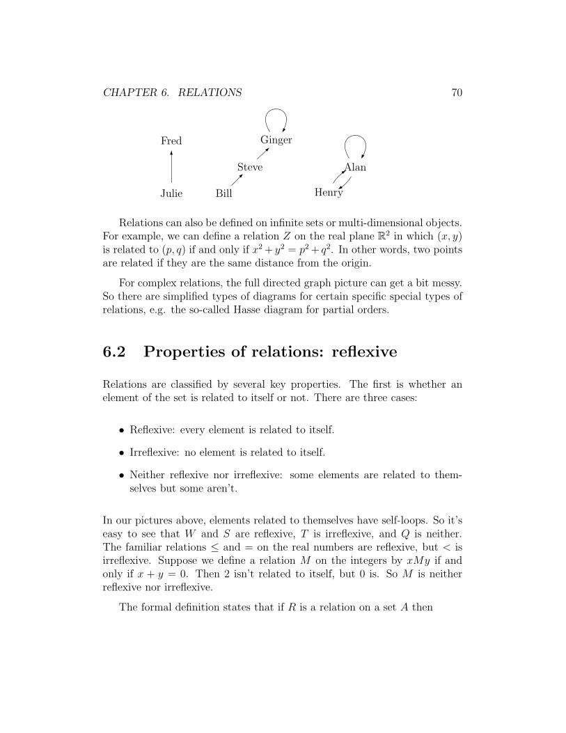
CHAPTER 6. RELATIONS 70
Fred Ginger
AlanSteve
Julie Bill Henry
Relations can also be defined on infinite sets or multi-dimensional objects.For example, we can define a relation Z on the real plane R2 in which (x, y)is related to (p, q) if and only if x2+ y2 = p2+ q2. In other words, two pointsare related if they are the same distance from the origin.
For complex relations, the full directed graph picture can get a bit messy.So there are simplified types of diagrams for certain specific special types ofrelations, e.g. the so-called Hasse diagram for partial orders.
6.2 Properties of relations: reflexive
Relations are classified by several key properties. The first is whether anelement of the set is related to itself or not. There are three cases:
• Reflexive: every element is related to itself.
• Irreflexive: no element is related to itself.
• Neither reflexive nor irreflexive: some elements are related to them-selves but some aren’t.
In our pictures above, elements related to themselves have self-loops. So it’seasy to see that W and S are reflexive, T is irreflexive, and Q is neither.The familiar relations ≤ and = on the real numbers are reflexive, but < isirreflexive. Suppose we define a relation M on the integers by xMy if andonly if x + y = 0. Then 2 isn’t related to itself, but 0 is. So M is neitherreflexive nor irreflexive.
The formal definition states that if R is a relation on a set A then
CHAPTER 6. RELATIONS 71
• R is reflexive if xRx for all x ∈ A.
• R is irreflexive if x 6Rx for all x ∈ A.
Notice that irreflexive is not the negation of reflexive. The negation ofreflexive would be:
• not reflexive: there is an x ∈ A, x 6Ry
6.3 Symmetric and antisymmetric
Another important property of a relation is whether the order matters withineach pair. That is, if xRy is in R, is it always the case that yRx? If this istrue, then the relation is called symmetric.
In a graph picture of a symmetric relation, a pair of elements is eitherjoined by a pair of arrows going in opposite directions, or no arrows. In ourexamples with pictures above, only S is symmetric.
Relations that resemble equality are normally symmetric. For example,the relation X on the integers defined by xXy iff |x| = |y| is symmetric. Sois the relation N on the real plane defined by (x, y)N(p, q)) iff (x−p)2+(y−q)2 ≤ 25 (i.e. the two points are no more than 5 units apart).
Relations that put elements into an order, like ≤ or divides, have a differ-ent property called antisymmetry. A relation is antisymmetric if two distinct1
elements are never related in both directions. In a graph picture of an an-tisymmetric relation, a pair of points may be joined by a single arrow, ornot joined at all. They are never joined by arrows in both directions. In ourpictures above, W and T are antisymmetric.
As with reflexivity, there are mixed relations that have neither property.So the relation Q above is neither symmetric nor antisymmetric.
If R is a relation on a set A, here’s the formal definition of what it meansfor R to be symmetric (which doesn’t contain anything particularly difficult):
1“Distinct” means not equal.

CHAPTER 6. RELATIONS 72
symmetric: for all x, y ∈ A, xRy implies yRx
There’s two ways to define antisymmetric. They are logically equivalentand you can pick whichever is more convenient for your purposes:
antisymmetric: for all x and y in A with x 6= y, if xRy, then y 6Rx
antisymmetric: for all x and y in A, if xRy and yRx, then x = y
To interpret the second definition, remember that when mathematicianspick two values x and y, they leave open the possibility that the two valuesare actually the same. In normal conversational English, if we mention twoobjects with different names, we normally mean to imply that they are differ-ent objects. This isn’t the case in mathematics. I find that the first definitionof antisymmetry is better for understanding the idea, but the second is moreuseful for writing proofs.
6.4 Transitive
The final important property of relations is transitivity. A relation R on aset A is transitive if
transitive: for all a, b, c ∈ A, ifaRb and bRc, then aRc
As we’ve seen earlier, transitivity holds for a broad range of familiarnumerical relations such as <, =, divides, and set inclusion. For example,for real numbers, if x < y and y < z, then x < z. Similarly, if x|y and y|z,then x|z. For sets, X ⊆ Y and Y ⊆ Z implies that X ⊆ Z.
If we look at graph pictures, transitivity means that whenever there is anindirect path from x to y then there must also be a direct arrow from x toy. This is true for S and B above, but not for W or Q.
We can also understand this by spelling out what it means for a relationR on a set A not to be transitive:
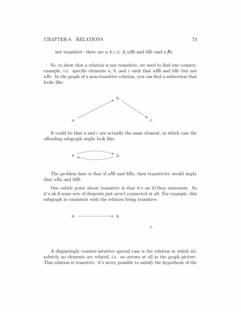
CHAPTER 6. RELATIONS 73
not transitive: there are a, b, c ∈ A, aRb and bRc and a 6Rc
So, to show that a relation is not transitive, we need to find one counter-example, i.e. specific elements a, b, and c such that aRb and bRc but notaRc. In the graph of a non-transitive relation, you can find a subsection thatlooks like:
a
b
c
It could be that a and c are actually the same element, in which case theoffending subgraph might look like:
a b
The problem here is that if aRb and bRa, then transitivity would implythat aRa and bRb.
One subtle point about transitive is that it’s an if/then statement. Soit’s ok if some sets of elements just aren’t connected at all. For example, thissubgraph is consistent with the relation being transitive.
a b
c
A disgustingly counter-intuitive special case is the relation in which ab-solutely no elements are related, i.e. no arrows at all in the graph picture.This relation is transitive. it’s never possible to satisfy the hypothesis of the
CHAPTER 6. RELATIONS 74
definition of transitive. It’s also symmetric, for the same reason. And, oddlyenough, antisymmetric. All of these properties hold via vacuous truth.
Vacuous truth doesn’t apply to reflexive and irreflexive, because they areunconditional requirements, not if/then statements. So this empty relationis irreflexive and not reflexive.
6.5 Types of relations
Now that we have these basic properties defined, we can define some impor-tant types of relations. Three of these are ordering relations:
• A partial order is a relation that is reflexive, antisymmetric, andtransitive.
• A linear order (also called a total order) is a partial order in whichevery pair of elements are comparable. That is, for every pair x, y,x ≥ y or y ≥ x.
• A strict partial order is a relation that is irreflexive, antisymmetric,and transitive.
A linear order is like the normal ≤ ordering on the integers. A partialorder is similar, but there are some pairs of elements which aren’t orderedwith respect to each other. For example, the divides relation on the integersis a partial order but not a linear order, because (for example) 5 is neither afactor nor a multiple of 7. A strict partial order is like a partial order, exceptthat objects are not related to themselves, the relation T in section 6.1 is astrict partial order.
The fourth type of relation is an equivalence relation:
Definition: An equivalence relation is a relation that is reflex-ive, symmetric, and transitive.
These three properties create a well-behaved notation of equivalence orcongruence for a set of objects, like congruence mod k on the set of integers.
CHAPTER 6. RELATIONS 75
In particular, if R is an equivalence relation on a set A and x is an elementof A, we can define the equivalence class of x to be the set of all elementsrelated to x. That is
[x]R = {y ∈ A | xRy}
When the relation is clear from the context (as when we discussed congruencemod k), we frequently omit the subscript on the square brackets.
For example, we saw the relation Z on the real plane R2, where (x, y)Z(p, q)if and only if x2 + y2 = p2 + q2. Then [(0, 1)]Z contains all the points relatedto (0, 1), i.e. the unit circle.
6.6 Proving that a relation is an equivalence
relation
Let’s see how to prove that a new relation is an equivalence relation. Theseproofs are usually very mechanical. For example, let F be the set of allfractions, i.e.
F = {pq| p, q ∈ Z and q 6= 0}
Fractions aren’t the same thing as rational numbers, because each rationalnumber is represented by many fractions. We consider two fractions to beequivalent, i.e. represent the same rational number, if xq = yp. So, we havean equivalence relation ∼ defined by: x
y∼ p
qif and only if xq = yp.
Let’s show that ∼ is an equivalence relation.
Proof: Reflexive: For any x and y, xy = xy. So the definition of∼ implies that x
y∼ x
y.
Symmetric: if xy∼ p
qthen xq = yp, so yp = xq, so py = qx, which
implies that p
q∼ x
y.
Transitive: Suppose that xy∼ p
qand p
q∼ s
t. By the definition of
∼, xq = yp and pt = qs. So xqt = ypt and pty = qsy. Since

CHAPTER 6. RELATIONS 76
ypt = pty, this means that xqt = qsy. Cancelling out the q’s, weget xt = sy. By the definition of ∼, this means that x
y∼ s
t.
Since ∼ is reflexive, symmetric, and transitive, it is an equivalencerelation.
Notice that the proof has three sub-parts, each showing one of the keyproperties. Each part involves using the definition of the relation, plus asmall amount of basic math. The reflexive case is very short. The symmetriccase is often short as well. Most of the work is in the transitive case.
6.7 Proving antisymmetry
Here’s another example of a relation, this time an order (not an equivalence)relation. Consider the set of intervals on the real line J = {(a, b) | a, b ∈R and a < b}. Define the containment relation C as follows:
(a, b) C (c, d) if and only if a ≤ c and d ≤ b
To show that C is a partial order, we’d need to show that it’s reflex-ive, antisymmetric, and transitive. We’ve seen how to prove two of theseproperties. Let’s see how to do a proof of antisymmetry.
For proving antisymmetry, it’s typically easiest to use this form of thedefinition of antisymmetry: if xRy and yRx, then x = y. Notice that C is arelation on intervals, i.e. pairs of numbers, not single numbers. Substitutingthe definition of C into the definition of antisymmetry, we need to show that
For any intervals (a, b) and (c, d), if (a, b) C (c, d) and (c, d) C (a, b),then (a, b) = (c, d).
So, suppose that we have two intervals (a, b) and (c, d) such that (a, b) C (c, d)and (c, d) C (a, b). By the definition of C, (a, b) C (c, d) implies that a ≤ cand d ≤ b. Similarly, (c, d) C (a, b) implies that c ≤ a and b ≤ d.
Since a ≤ c and c ≤ a, a = c. Since d ≤ b and b ≤ d, b = d. So(a, b) = (c, d).

Chapter 7
Functions and onto
This chapter covers functions, including function composition and what itmeans for a function to be onto. In the process, we’ll see what happens whentwo dissimilar quantifiers are nested.
7.1 Functions
We’re all familiar with functions from high school and calculus. However,these prior math courses concentrate on functions whose inputs and outputsare numbers, defined by an algebraic formula such as f(x) = 2x+3. We’ll beusing a broader range of functions, whose input and/or output values maybe integers, strings, characters, and the like.
Suppose that A and B are sets, then a function f from A to B is anassignment of exactly one element of B (i.e. the output value) to each elementof A (i.e. the input value). A is called the domain of f and B is called theco-domain. All of this information can be captured in the shorthand typesignature: f : A → B. If x is an element of A, then the value f(x) is alsoknown as the image of x.
For example, suppose P is a set of five people:
P = {Margaret,Tom,Chen,LaSonya,Emma}
77
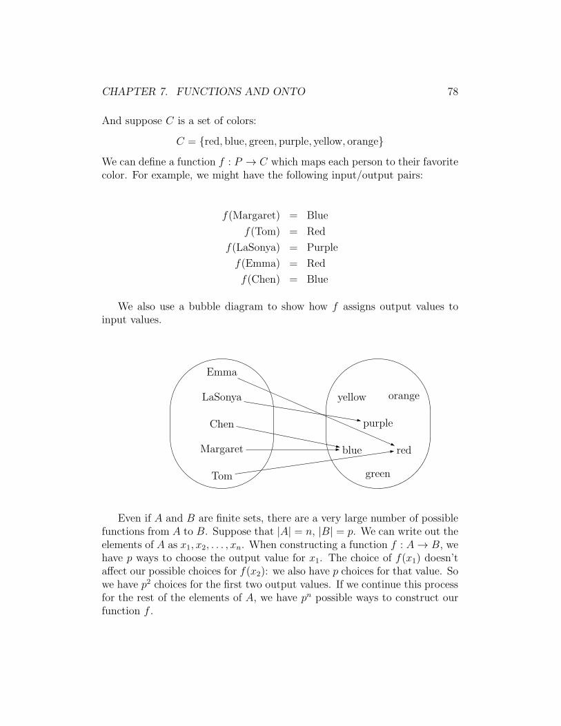
CHAPTER 7. FUNCTIONS AND ONTO 78
And suppose C is a set of colors:
C = {red, blue, green, purple, yellow, orange}We can define a function f : P → C which maps each person to their favoritecolor. For example, we might have the following input/output pairs:
f(Margaret) = Blue
f(Tom) = Red
f(LaSonya) = Purple
f(Emma) = Red
f(Chen) = Blue
We also use a bubble diagram to show how f assigns output values toinput values.
Margaret
Tom
Chen
LaSonya
Emma
blue red
green
purple
yellow orange
Even if A and B are finite sets, there are a very large number of possiblefunctions from A to B. Suppose that |A| = n, |B| = p. We can write out theelements of A as x1, x2, . . . , xn. When constructing a function f : A → B, wehave p ways to choose the output value for x1. The choice of f(x1) doesn’taffect our possible choices for f(x2): we also have p choices for that value. Sowe have p2 choices for the first two output values. If we continue this processfor the rest of the elements of A, we have pn possible ways to construct ourfunction f .

CHAPTER 7. FUNCTIONS AND ONTO 79
For any set A, the identity function idA maps each value in A to itself.That is, idA : A → A and idA(x) = x.
7.2 When are functions equal?
Notice that the domain and co-domain are an integral part of the definitionof the function. To be equal, two functions must (obviously) assign the sameoutput value to each input value. But, in addition, they must have the sametype signature.
For example, suppose D is a slightly smaller set of colors:
D = {red, blue, purple}
Then the function g : P → D shown below is not equal to the function ffrom section 7.1, even though g(x) = f(x) for every x in P .
Margaret
Tom
Chen
LaSonya
Emma
blue red
purple
Similarly, the following definitions describe quite different functions, eventhough they are based on the same equation.
• f : N → N such that f(x) = 2x.
• f : R → R such that f(x) = 2x.
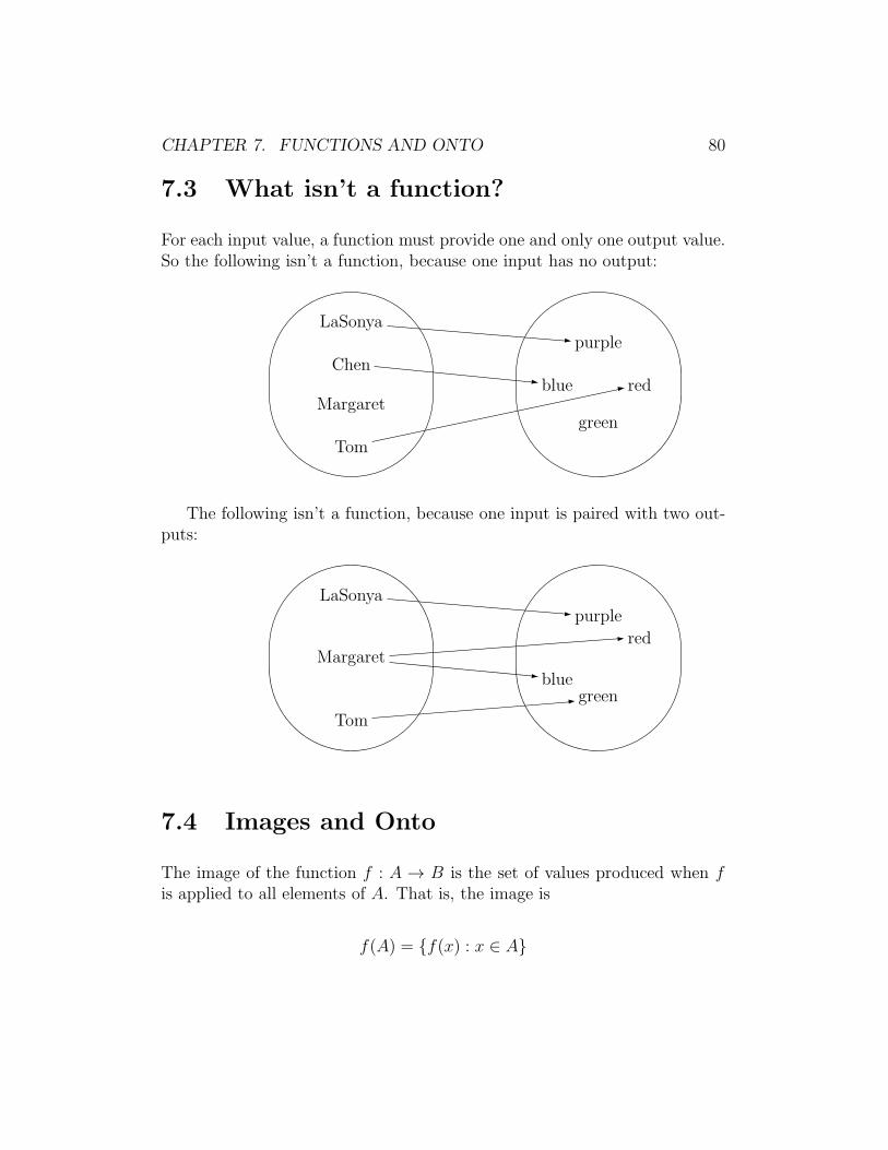
CHAPTER 7. FUNCTIONS AND ONTO 80
7.3 What isn’t a function?
For each input value, a function must provide one and only one output value.So the following isn’t a function, because one input has no output:
Margaret
Tom
Chen
LaSonya
blue red
purple
green
The following isn’t a function, because one input is paired with two out-puts:
Margaret
Tom
LaSonya
blue
red
purple
green
7.4 Images and Onto
The image of the function f : A → B is the set of values produced when fis applied to all elements of A. That is, the image is
f(A) = {f(x) : x ∈ A}
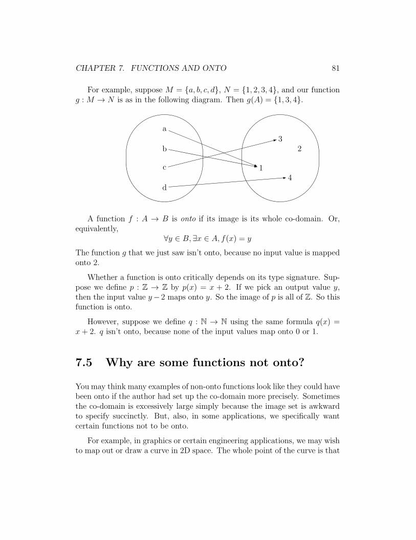
CHAPTER 7. FUNCTIONS AND ONTO 81
For example, suppose M = {a, b, c, d}, N = {1, 2, 3, 4}, and our functiong : M → N is as in the following diagram. Then g(A) = {1, 3, 4}.
a
b
c
d
1
23
4
A function f : A → B is onto if its image is its whole co-domain. Or,equivalently,
∀y ∈ B, ∃x ∈ A, f(x) = y
The function g that we just saw isn’t onto, because no input value is mappedonto 2.
Whether a function is onto critically depends on its type signature. Sup-pose we define p : Z → Z by p(x) = x + 2. If we pick an output value y,then the input value y−2 maps onto y. So the image of p is all of Z. So thisfunction is onto.
However, suppose we define q : N → N using the same formula q(x) =x+ 2. q isn’t onto, because none of the input values map onto 0 or 1.
7.5 Why are some functions not onto?
You may think many examples of non-onto functions look like they could havebeen onto if the author had set up the co-domain more precisely. Sometimesthe co-domain is excessively large simply because the image set is awkwardto specify succinctly. But, also, in some applications, we specifically wantcertain functions not to be onto.
For example, in graphics or certain engineering applications, we may wishto map out or draw a curve in 2D space. The whole point of the curve is that
CHAPTER 7. FUNCTIONS AND ONTO 82
it occupies only part of 2D and it is surrounded by whitespace. These curvesare often specified “parametrically,” using functions that map into, but notonto, 2D.
For example, we can specify a (unit) circle as the image of a functionf : [0, 1] → R2 defined by f(x) = (cos 2πx, sin 2πx). If you think of the inputvalues as time, then f shows the track of a pen or robot as it goes aroundthe circle. The cosine and sine are the x and y coordinates of its position.The 2π multiplier simply puts the input into the right range so that we’llsweep exactly once around the circle (assuming that sine and cosine taketheir inputs in radians).
7.6 Negating onto
To understand the concept of onto, it may help to think about what itmeans for a function not to be onto. This is our first example of negating astatement involving two nested (different) quantifiers. Our definition of ontois
∀y ∈ B, ∃x ∈ A, f(x) = y
So a function f is not onto if
¬∀y ∈ B, ∃x ∈ A, f(x) = y
To negate this, we proceed step-by-step, moving the negation inwards.You’ve seen all the identities involved, so this is largely a matter of beingcareful.
¬∀y ∈ B, ∃x ∈ A, f(x) = y
≡ ∃y ∈ B,¬∃x ∈ A, f(x) = y
≡ ∃y ∈ B, ∀x ∈ A,¬(f(x) = y)
≡ ∃y ∈ B, ∀x ∈ A, f(x) 6= y

CHAPTER 7. FUNCTIONS AND ONTO 83
So, if we want to show that f is not onto, we need to find some value yin B, such that no matter which element x you pick from A, f(x) isn’t equalto y.
7.7 Nested quantifiers
Notice that the definition of onto combines a universal and an existentialquantifier, with the scope of one including the scope of the other. These arecalled nested quantifiers. When quantifiers are nested, the meaning of thestatement depends on the order of the two quantifiers.
For example,
For every person p in the Fleck family, there is a toothbrush tsuch that p brushes their teeth with t.
This sentence asks you to consider some random Fleck. Then, given thatchoice, it asserts that they have a toothbrush. The toothbrush is chosenafter we’ve picked the person, so the choice of toothbrush can depend on thechoice of person. This doesn’t absolutely force everyone to pick their owntoothbrush. (For a brief period, two of my sons were using the same onebecause they got confused.) However, at least this statement is consistentwith each person having their own toothbrush.
Suppose now that we swap the order of the quantifiers, to get
There is a toothbrush t, such that for every person p in the Fleckfamily, p brushes their teeth with t.
In this case, we’re asked to choose a toothbrush t first. Then we’re assert-ing that every Fleck uses this one fixed toothbrush t. Eeeuw! That wasn’twhat we wanted to say!
We do want the existential quantifier first when there’s a single objectthat’s shared among the various people, as in:
CHAPTER 7. FUNCTIONS AND ONTO 84
There is a stove s, such that for every person p in the Fleck family,p cooks his food on s.
Notice that this order issue only appears when a statement a mixture ofexistential and universal quantifiers. If all the quantifiers are existential, orif all the quantifiers are universal, the order doesn’t matter.
To take a more mathematical example, let’s look back at modular arith-metic. Two numbers x and y are multiplicative inverses if xy = yx = 1. Inthe integers Z, only 1 has a multiplicative inverse. However, in Zk, manyother integers have inverses. For example, if k = 7, then [3][5] = [1]. So [3]and [5] are inverses.
For certain values of k every non-zero element of Zk has an inverse.1 Youcan verify that this is true for Z7: [3] and [5] are inverses, [2] and [4] areinverses, [1] is its own inverse, and [6] is its own inverse. So we can say that
∀ non-zero x ∈ Z7, ∃y ∈ Z7, xy = yx = 1
Notice that we’ve put the universal quantifier outside the existential one,so that each number gets to pick its own inverse. Reversing the order of thequantifers would give us the following statement:
∃y ∈ Z7, ∀ non-zero x ∈ Z7, xy = yx = 1
This version isn’t true, because you can’t pick one single number thatworks as an inverse for all the rest of the non-zero numbers, even in modulararithmetic.
However, we do want the existential quantifier first in the following claim,because 0y = y0 = 0 for every y ∈ Z7.
∃x ∈ Z7, ∀y ∈ Z7, xy = yx = x
1Can you figure out which values of k have this property?
CHAPTER 7. FUNCTIONS AND ONTO 85
7.8 Proving that a function is onto
Now, consider this claim:
Claim 32 Define the function g from the integers to the integers by theformula g(x) = x− 8. g is onto.
Proof: We need to show that for every integer y, there is aninteger x such that g(x) = y.
So, let y be some arbitrary integer. Choose x to be (y + 8).x is an integer, since it’s the sum of two integers. But theng(x) = (y+8)− 8 = y, so we’ve found the required pre-image fory and our proof is done.
For some functions, several input values map onto a single output value.In that case, we can choose any input value in our proof, typically whicheveris easiest for the proof-writer. For example, suppose we had g : Z → Z suchthat g(x) = ⌊x
2⌋. To show that g is onto, we’re given an output value x and
need to find the corresponding input value. The simplest choice would be 2xitself. But you could also pick 2x+ 1.
Suppose we try to build such a proof for a function that isn’t onto, e.g.f : Z → Z such that f(x) = 3x+ 2.
Proof: We need to show that for every integer y, there is aninteger x such that f(x) = y.
So, let y be some arbitrary integer. Choose x to be (y−2)3
. . . .
If f was a function from the reals to the reals, we’d be ok at this point,because x would be a good pre-image for y. However, f ’s inputs are declaredto be integers. For many values of y, (y−2)
3isn’t an integer. So it won’t work
as an input value for f .

CHAPTER 7. FUNCTIONS AND ONTO 86
7.9 A 2D example
Here’s a sample function whose domain is 2D. Let f : Z2 → Z be defined byf(x, y) = x+ y. I claim that f is onto.
First, let’s make sure we know how to read this definition. f : Z2 isshorthand for Z× Z, which is the set of pairs of integers. So f maps a pairof integers to a single integer, which is the sum of the two coordinates.
To prove that f is onto, we need to pick some arbitrary element y in theco-domain. That is to say, y is an integer. Then we need to find a samplevalue in the domain that maps onto y, i.e. a “preimage” of y. At this point,it helps to fiddle around on our scratch paper, to come up with a suitablepreimage. In this case, (0, y) will work nicely. So our proof looks like:
Proof: Let y be an element of Z. Then (0, y) is an element off : Z2 and f(0, y) = 0 + y = y. Since this construction will workfor any choice of y, we’ve shown that f is onto.
Notice that this function maps many input values onto each output value.So, in our proof, we could have used a different formula for finding the inputvalue, e.g. (1, y − 1) or (y, 0). A proof writer with a sense of humor mightuse (342, y − 342).
7.10 Composing two functions
Suppose that f : A → B and g : B → C are functions. Then g ◦ f is thefunction from A to C defined by (g ◦ f)(x) = g(f(x)). Depending on theauthor, this is either called the composition of f and g or the composition ofg and f . The idea is that you take input values from A, run them throughf , and then run the result of that through g to get the final output value.
Take-home message: when using function composition, look at the au-thor’s shorthand notation rather than their mathematical English, to beclear on which function gets applied first.
In this definition, notice that g came first in (g ◦ f)(x) and g also comesfirst in g(f(x)). I.e. unlike f(g(x)) where f comes first. The trick for

CHAPTER 7. FUNCTIONS AND ONTO 87
remembering this definition is to remember that f and g are in the sameorder on the two sides of the defining equation.
For example, suppose we define two functions f and g from the integersto the integers by:
f(x) = 3x+ 7
g(x) = x− 8
Since the domains and co-domains for both functions are the integers, wecan compose the two functions in both orders. But two composition ordersgive us different functions:
(f ◦ g)(x) = f(g(x)) = 3g(x) + 7 = 3(x− 8) + 7 = 3x− 24 + 7 = 3x− 17
(g ◦ f)(x) = g(f(x)) = f(x)− 8 = (3x+ 7)− 8 = 3x− 1
Frequently, the declared domains and co-domains of the two functionsaren’t all the same, so often you can only compose in one order. For example,consider the function h : {strings} → Z which maps a string x onto its lengthin characters. (E.g. h(Margaret) = 8.) Then f ◦ h exists but (h ◦ f) doesn’texist because f produces numbers and the inputs to h are supposed to bestrings.
7.11 A proof involving composition
Let’s show that onto-ness works well with function composition. Specifically:
Claim 33 For any sets A, B, and C and for any functions f : A → B andg : B → C, if f and g are onto, then g ◦ f is also onto.
Proof: Let A, B, and C be sets. Let f : A → B and g : B → Cbe functions. Suppose that f and g are onto.

CHAPTER 7. FUNCTIONS AND ONTO 88
We need to show that g ◦ f is onto. That is, we need to showthat for any element x in C, there is an element y in A such that(g ◦ f)(y) = x.
So, pick some element x in C. Since g is onto, there is an elementz in B such that g(z) = x. Since f is onto, there is an element yin A such that f(y) = z.
Substituting the value f(y) = z into the equation g(z) = x, weget g(f(y)) = x. That is, (g ◦ f)(y) = x. So y is the element ofA we needed to find.
7.12 Variation in terminology
A function is often known as a “map” and “surjective” is often used as asynonym for “onto.” The image of a function is sometimes written Im(f).The useful term “type signature” is not traditional in pure mathematics,though it’s in wide use in computer science.
The term “range” is a term that has become out-dated in mathematics.Depending on the author, it may refer to either the image or the co-domainof a function, which creates confusion. Avoid using it.
Some authors write gf rather than g ◦ f for the composition of two func-tions. Also, some authors define g ◦ f such that g ◦ f(x) = f(g(x)), i.e. theopposite convention from what we’re using.
Chapter 8
Functions and one-to-one
In this chapter, we’ll see what it means for a function to be one-to-one andbijective. This general topic includes counting permutations and comparingsizes of finite sets (e.g. the pigeonhole principle). We’ll also see the methodof adding stipulations to a proof “without loss of generality” as well as thetechnique of proving an equality via upper and lower bounds.
8.1 One-to-one
Suppose that f : A → B is a function from A to B. If we pick a value y ∈ B,then x ∈ A is a pre-image of y if f(x) = y. Notice that I said a pre-imageof y, not the pre-image of y, because y might have more than one preimage.For example, in the following function, 1 and 2 are pre-images of 1, 4 and 5are pre-images of 4, 3 is a pre-image of 3, and 2 has no preimages.
89
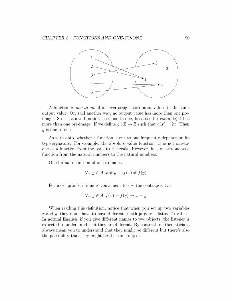
CHAPTER 8. FUNCTIONS AND ONE-TO-ONE 90
1
2
3
4
5
1
23
4
A function is one-to-one if it never assigns two input values to the sameoutput value. Or, said another way, no output value has more than one pre-image. So the above function isn’t one-to-one, because (for example) 4 hasmore than one pre-image. If we define g : Z → Z such that g(x) = 2x. Theng is one-to-one.
As with onto, whether a function is one-to-one frequently depends on itstype signature. For example, the absolute value function |x| is not one-to-one as a function from the reals to the reals. However, it is one-to-one as afunction from the natural numbers to the natural numbers.
One formal definition of one-to-one is:
∀x, y ∈ A, x 6= y → f(x) 6= f(y)
For most proofs, it’s more convenient to use the contrapositive:
∀x, y ∈ A, f(x) = f(y) → x = y
When reading this definition, notice that when you set up two variablesx and y, they don’t have to have different (math jargon: “distinct”) values.In normal English, if you give different names to two objects, the listener isexpected to understand that they are different. By contrast, mathematiciansalways mean you to understand that they might be different but there’s alsothe possibility that they might be the same object.
CHAPTER 8. FUNCTIONS AND ONE-TO-ONE 91
8.2 Bijections
If a function f is both one-to-one and onto, then each output value hasexactly one pre-image. So we can invert f , to get an inverse function f−1. Afunction that is both one-to-one and onto is called bijective or a bijection. Iff maps from A to B, then f−1 maps from B to A.
Suppose that A and B are finite sets. Constructing an onto functionfrom A to B is only possible when A has at least as many elements as B.Constructing a one-to-one function from A to B requires that B have at leastas many values as A. So if there is a bijection between A and B, then the twosets must contain the same number of elements. As we’ll see later, bijectionsare also used to define what it means for two infinite sets to be the “samesize.”
8.3 Pigeonhole Principle
Suppose that A contains more elements than B. Then it’s impossible toconstruct a bijection fromA to B, because two elements of Amust be mappedto the same element of B. If we rephrase this in terms of putting labels onobjects, we get the following Pigeonhole Principle:
Pigeonhole principle: Suppose you have n objects and assignk labels to these objects. If n > k, then two objects must get thesame label.
For example, if you have 8 playing cards and the cards come in five colors,then at least two of the cards share the same color. Or, if you have a 30-character string containing lowercase letters, it must contain some duplicateletters, because 26 is smaller than 30.
The pigeonhole principle (like many superheros) has a dual identity.When you’re told to apply it to some specific objects and labels, it’s ob-vious how to do so. However, it is often pulled out of nowhere as a clevertrick in proofs, where you would have never suspected that it might be useful.Such proofs are easy to read, but sometimes hard to come up with.
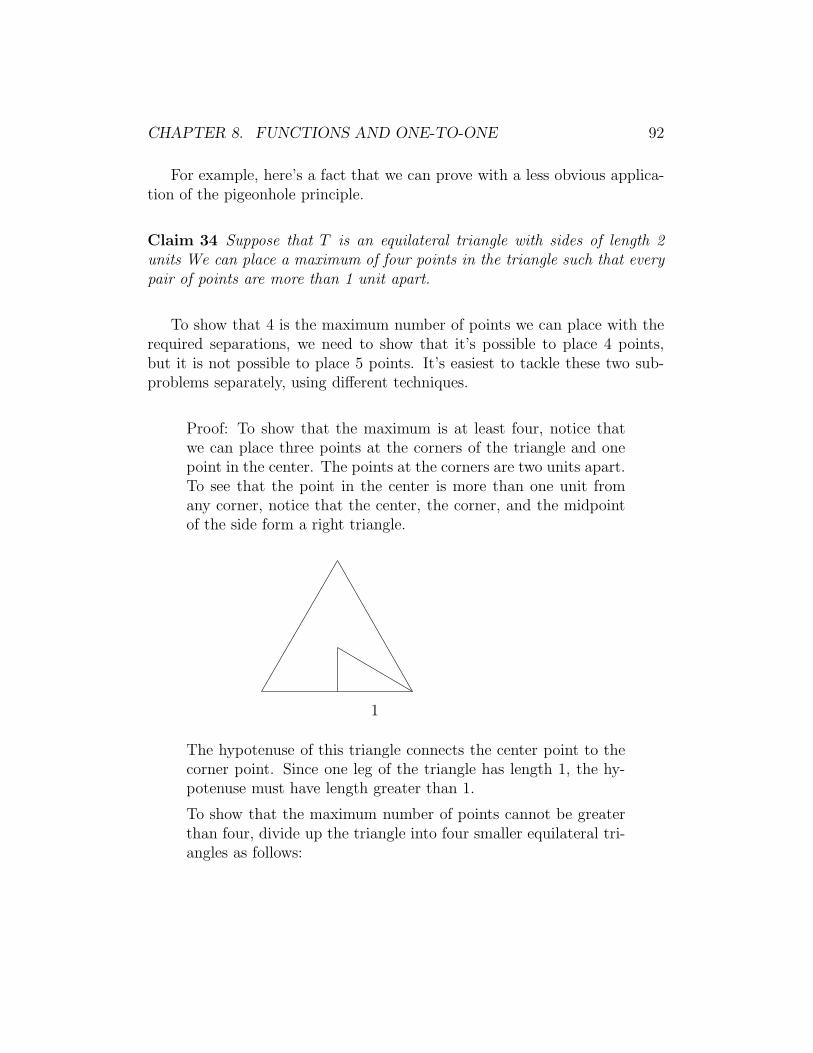
CHAPTER 8. FUNCTIONS AND ONE-TO-ONE 92
For example, here’s a fact that we can prove with a less obvious applica-tion of the pigeonhole principle.
Claim 34 Suppose that T is an equilateral triangle with sides of length 2units We can place a maximum of four points in the triangle such that everypair of points are more than 1 unit apart.
To show that 4 is the maximum number of points we can place with therequired separations, we need to show that it’s possible to place 4 points,but it is not possible to place 5 points. It’s easiest to tackle these two sub-problems separately, using different techniques.
Proof: To show that the maximum is at least four, notice thatwe can place three points at the corners of the triangle and onepoint in the center. The points at the corners are two units apart.To see that the point in the center is more than one unit fromany corner, notice that the center, the corner, and the midpointof the side form a right triangle.
1
The hypotenuse of this triangle connects the center point to thecorner point. Since one leg of the triangle has length 1, the hy-potenuse must have length greater than 1.
To show that the maximum number of points cannot be greaterthan four, divide up the triangle into four smaller equilateral tri-angles as follows:

CHAPTER 8. FUNCTIONS AND ONE-TO-ONE 93
Suppose we tried to place five or more points into the big trian-gle. Since there are only four small triangles, by the pigeonholeprinciple, some small triangle would have to contain at least twopoints. But since the small triangle has side length only 1, thesepoints can’t be separated by more than one unit.
The tricky part of this proof isn’t the actual use of the pigeonhole prin-ciple. Rather, it’s the setup steps, e.g. dividing up the triangle, that got usto the point where the pigeonhole principle could be applied. This is typicalof harder pigeonhole principle proofs.
8.4 Permutations
Now, suppose that |A| = n = |B|. We can construct a number of one-to-onefunctions from A to B. How many? Suppose that A = {x1, x2, . . . , xn}.We have n ways to choose the output value for x1. But that choice uses upone output value, so we have only n − 1 choices for the output value of x2.Continuing this pattern, we have n(n− 1)(n− 2) . . . 2 · 1 (n! for short) waysto construct our function.
Similarly, suppose we have a group of n dragon figurines that we’d like toarrange on the mantlepiece. We need to construct a map from positions onthe mantlepiece to dragons. There are n! ways to do this. An arrangementof n objects in order is called a permutation of the n objects.
More frequently, we need to select an ordered list of k objects from alarger set of n objects. For example, we have 30 dragon figurines but spacefor only 10 on our mantlepiece. Then we have 30 choices for the first figurine,

CHAPTER 8. FUNCTIONS AND ONE-TO-ONE 94
29 for the second, and so forth down to 21 choices for the last one. Thus wehave 30 · 29 · . . . 21 ways to decorate the mantlepiece.
In general, an ordered choice of k objects from a set of n objects is knownas a k-permutation of the n objects. There are n(n−1) . . . (n−k+1) = n!
(n−k)!
different k-permutations of n objects. This number is called P (n, k). P (n, k)is also the number of one-to-one functions from a set of k objects to a set ofn objects.
8.5 Further applications of permutations
Many real-world counting problems can be solved with the permutations for-mulas, but some problems require a bit of adaptation. For example, supposethat 7 adults and 3 kids need to get in line at the airport. Also suppose thatwe can’t put two children next to each other, because they will fight.
The trick for this problem is to place the 7 adults in line, with gapsbetween them. Each gap might be left empty or filled with one kid. Thereare 8 gaps, into which we have to put the 3 kids. So, we have 7! ways toassign adults to positions. Then we have 8 gaps in which we can put kid A,7 for kid B, and 6 for kid C. That is 7! · 8 · 7 · 6 ways to line them all up.
Now, let’s suppose that we have a set of 7 scrabble tiles and we wouldlike to figure out how many different letter strings we can make out of them.We could almost use the permutations formula, except that some of thetiles might contain the same letter. For example, suppose that the tiles are:C,O, L, L, E,G,E.
First, let’s smear some dirt on the duplicate tiles, so we can tell thetwo copies apart: C,O, L1, L2, E1, G, E2. Then we would calculate 7! per-mutations of this list. However, in terms of our original problem, this isdouble-counting some possibilities, because we don’t care about the differ-ence between duplicates like L1 and L2. So we need to divide out by thenumber of ways we can permute the duplicates. In this case, we have 2! waysto permute the l’s and 2! ways to permute the e’s. So the true number oforderings of L is 7!
2!2!.
Similarly, the number of reorderings of J = (a, p, p, l, e, t, r, e, e, s) is 10!2!3!
.
CHAPTER 8. FUNCTIONS AND ONE-TO-ONE 95
In general, suppose we have n objects, where n1 are of type 1, n2 are oftype 2, and so forth through nk are of type k. Then the number of ways toorder our list of objects is n!
n1!n2!...nk!.
8.6 Proving that a function is one-to-one
Now, let’s move on to examples of how to prove that a specific function isone-to-one.
Claim 35 Let f : Z → Z be defined by f(x) = 3x+ 7. f is one-to-one.
Let’s prove this using our definition of one-to-one.
Proof: We need to show that for every integers x and y, f(x) =f(y) → x = y.
So, let x and y be integers and suppose that f(x) = f(y). Weneed to show that x = y.
We know that f(x) = f(y). So, substituting in our formula for f ,3x+ 7 = 3y + 7. So 3x = 3y and therefore x = y, by high schoolalgebra. This is what we needed to show.
When we pick x and y at the start of the proof, notice that we haven’tspecified whether they are the same number or not. Mathematical conventionleaves this vague, unlike normal English where the same statement wouldstrongly suggest that they were different.
8.7 Composition and one-to-one
Like onto, one-to-one works well with function composition. Specifically:
Claim 36 For any sets A, B, and C and for any functions f : A → B andg : B → C, if f and g are one-to-one, then g ◦ f is also one-to-one.
CHAPTER 8. FUNCTIONS AND ONE-TO-ONE 96
We can prove this with a direct proof, by being systematic about using ourdefinitions and standard proof outlines. First, let’s pick some representativeobjects of the right types and assume everything in our hypothesis.
Proof: Let A, B, and C be sets. Let f : A → B and g : B → Cbe functions. Suppose that f and g are one-to-one.
We need to show that g ◦ f is one-to-one.
To show that g ◦ f is one-to-one, we need to pick two elements x andy in its domain, assume that their output values are equal, and then showthat x and y must themselves be equal. Let’s splice this into our draft proof.Remember that the domain of g ◦ f is A and its co-domain is C.
Proof: Let A, B, and C be sets. Let f : A → B and g : B → Cbe functions. Suppose that f and g are one-to-one.
We need to show that g ◦ f is one-to-one. So, choose x and y inA and suppose that (g ◦ f)(x) = (g ◦ f)(y)We need to show that x = y.
Now, we need to apply the definition of function composition and the factthat f and g are each one-to-one:
Proof: Let A, B, and C be sets. Let f : A → B and g : B → Cbe functions. Suppose that f and g are one-to-one.
We need to show that g ◦ f is one-to-one. So, choose x and y inA and suppose that (g ◦ f)(x) = (g ◦ f)(y)Using the definition of function composition, we can rewrite thisas g(f(x)) = g(f(y)). Combining this with the fact that g isone-to-one, we find that f(x) = f(y). But, since f is one-to-one,this implies that x = y, which is what we needed to show.
CHAPTER 8. FUNCTIONS AND ONE-TO-ONE 97
8.8 Strictly increasing functions are one-to-
one
Now, let’s do a slightly trickier proof. First, a definition. Suppose that Aand B are sets of real numbers (e.g. the reals, the rationals, the integers).A function f : A → B is increasing if, for every x and y in A, x ≤ y impliesthat f(x) ≤ f(y). f is called strictly increasing if, for every x and y in A,x < y implies that f(x) < f(y).1
Claim 37 For any sets of real numbers A and B, if f is any strictly increas-ing function from A to B, then f is one-to-one.
A similar fact applies to strictly decreasing functions.
To prove this, we will restate one-to-one using the alternative, contrapos-itive version of its definition.
∀x, y ∈ A, x 6= y → f(x) 6= f(y)
Normally, this wouldn’t be a helpful move. The hypothesis involves anegative fact, whereas the other version of the definition has a positive hy-pothesis, normally a better place to start. But this is an atypical exampleand, in this case, the negative information turns out to be a good startingpoint.
Proof: Let A and B be sets of numbers and let f : A → B be astrictly increasing function. Let x and y be distinct elements ofA. We need to show that f(x) 6= f(y).
Since x 6= y, there’s two possibilities.
Case 1: x < y. Since f is strictly increasing, this implies thatf(x) < f(y). So f(x) 6= f(y)
Case 2: y < x. Since f is strictly increasing, this implies thatf(y) < f(x). So f(x) 6= f(y).
1In math, “strictly” is often used to exclude the possibility of equality.

CHAPTER 8. FUNCTIONS AND ONE-TO-ONE 98
In either case, we have that f(x) 6= f(y), which is what we neededto show.
The phrase “distinct elements of A” is math jargon for x 6= y.
When we got partway into the proof, we had the fact x 6= y which isn’teasy to work with. But the trichotomy axiom for real number states that forany x and y, we have exactly three possibilities: x = y, x < y, or y < x. Theconstraint that x 6= y eliminates one of these possibilities.
8.9 Making this proof more succinct
In this example, the proofs for the two cases are very, very similar. So we canfold the two cases together. Here’s one approach, which I don’t recommenddoing in the early part of this course but which will serve you well later on:
Proof: Let A and B be sets of numbers and let f : A → B be astrictly increasing function. Let x and y be distinct elements ofA. We need to show that f(x) 6= f(y).
Since x 6= y, there’s two possibilities.
Case 1: x < y. Since f is strictly increasing, this implies thatf(x) < f(y). So f(x) 6= f(y)
Case 2: y < x. Similar to case 1.
In either case, we have that f(x) 6= f(y), which is what we neededto show.
This method only works if you, and your reader, both agree that it’sobvious that the two cases are very similar and the proof will really be similar.Dangerous assumption right now. And we’ve only saved a small amount ofwriting, which isn’t worth the risk of losing points if the grader doesn’t thinkit was obvious.
But this simplification can be very useful in more complicated situationswhere you have may have lots of cases, the proof for each case is long, andthe proofs for different cases really are very similar.
CHAPTER 8. FUNCTIONS AND ONE-TO-ONE 99
Here’s another way to simplify our proof:
Proof: Let A and B be sets of numbers and let f : A → B be astrictly increasing function. Let x and y be distinct elements ofA. We need to show that f(x) 6= f(y).
We know that x 6= y, so either x < y or y < x. Without loss ofgenerality, assume that x < y.
Since f is strictly increasing, x < y implies that f(x) < f(y). Sof(x) 6= f(y), which is what we needed to show.
The phrase “without loss of generality” means that we are adding anadditional assumption to our proof but we claim it isn’t really adding anymore information. In this case, s and t are both arbitrary indices introducedat the same time. It doesn’t really matter which of them is called s and whichis called t. So if we happen to have chosen our names in an inconvenient order,we could simply swap the two names.
Simplifying a problem “without loss of generality” is a powerful but po-tentially dangerous proof technique. You’ll probably probably want to see afew times before you use it yourself. It’s actually used fairly often to simplifyproofs, so it has an abbreviation: WOLOG or WLOG.
8.10 Variation in terminology
The term “injective” is a synonym for one-to-one and one-to-one correspon-dence is a synonym for bijective. The phrase “by symmetry” is often usedin place of “without loss of generality.”
Chapter 9
Graphs
Graphs are a very general class of object, used to formalize a wide variety ofpractical problems in computer science. In this chapter, we’ll see the basicsof (finite) undirected graphs, including graph isomorphism, connectivity, andgraph coloring.
9.1 Graphs
A graph consists of a set of nodes V and a set of edges E. We’ll sometimesrefer to the graph as a pair of sets (V,E). Each edge in E joins two nodesin V . Two nodes connected by an edge are called neighbors or adjacent.
For example, here is a graph in which the nodes are Illinois cities and theedges are roads joining them:
100

CHAPTER 9. GRAPHS 101
Chicago
Springfield
Bloomington
Urbana Danville
Decatur
A graph edge can be traversed in both directions, as in this street example,i.e. the edges are undirected. When discussing relations earlier, we useddirected graphs, in which each edge had a specific direction. Unless weexplicitly state otherwise, a “graph” will always be undirected. Concepts forundirected graphs extend in straightforward ways to directed graphs.
When there is only one edge connecting two nodes x and y, we can namethe edge using the pair of nodes. We could call the edge xy or (since orderdoesn’t matter) yx or {x, y}. So, in the graph above, the Urbana-Danvilleedge connects the node Urbana and the node Danville.
In some applications, we need graphs in which two nodes are connectedby multiple edges, i.e. parallel edges with the same endpoints. For exam-ple, the following graph shows ways to travel among four cities in the SanFrancisco Bay Area. It has three edges from San Francisco to Oakland, repre-senting different modes of transportation. When multiple edges are present,we typically label the edges rather than trying to name edges by their end-points. This diagram also illustrates a loop edge which connects a node toitself.
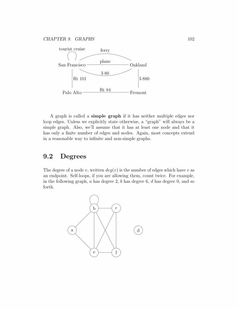
CHAPTER 9. GRAPHS 102
San Francisco Oakland
FremontPalo Alto
ferry
plane
I-80
tourist cruise
Rt 101
Rt 84
I-880
A graph is called a simple graph if it has neither multiple edges norloop edges. Unless we explicitly state otherwise, a “graph” will always be asimple graph. Also, we’ll assume that it has at least one node and that ithas only a finite number of edges and nodes. Again, most concepts extendin a reasonable way to infinite and non-simple graphs.
9.2 Degrees
The degree of a node v, written deg(v) is the number of edges which have v asan endpoint. Self-loops, if you are allowing them, count twice. For example,in the following graph, a has degree 2, b has degree 6, d has degree 0, and soforth.
a
b
e
c
d
f

CHAPTER 9. GRAPHS 103
Each edge contributes to two node degrees. So the sum of the degrees ofall the nodes is twice the number of edges. This is called the HandshakingTheorem and can be written as
∑
v∈V
deg(v) = 2|E|
This is a slightly different version of summation notation. We pick eachnode v in the set V , get its degree, and add its value into the sum. SinceV is finite, we could also have given names to the nodes v1, . . . , vn and thenwritten
n∑
k=1
vk ∈ V deg(v) = 2|E|
The advantage to the first, set-based, style is that it generalizes well tosituations involving infinite sets.
9.3 Complete graphs
Several special types of graphs are useful as examples. First, the completegraph on n nodes (shorthand name Kn), is a graph with n nodes in whichevery node is connected to every other node. K5 is shown below.
a
b c
d e
To calculate the number of edges in Kn, think about the situation fromthe perspective of the first node. It is connected to n− 1 other nodes. If welook at the second node, it adds n − 2 more connections. And so forth. Sowe have
∑n
k=1(n− k) =∑n−1
k=0 k = n(n−1)2
edges.
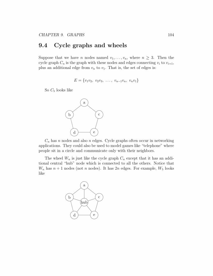
CHAPTER 9. GRAPHS 104
9.4 Cycle graphs and wheels
Suppose that we have n nodes named v1, . . . , vn, where n ≥ 3. Then thecycle graph Cn is the graph with these nodes and edges connecting vi to vi+1,plus an additional edge from vn to v1. That is, the set of edges is:
E = {v1v2, v2v3, . . . , vn−1vn, vnv1}
So C5 looks like
a
b c
d e
Cn has n nodes and also n edges. Cycle graphs often occur in networkingapplications. They could also be used to model games like “telephone” wherepeople sit in a circle and communicate only with their neighbors.
The wheel Wn is just like the cycle graph Cn except that it has an addi-tional central “hub” node which is connected to all the others. Notice thatWn has n + 1 nodes (not n nodes). It has 2n edges. For example, W5 lookslike
a
b c
d e
hub
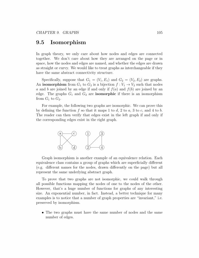
CHAPTER 9. GRAPHS 105
9.5 Isomorphism
In graph theory, we only care about how nodes and edges are connectedtogether. We don’t care about how they are arranged on the page or inspace, how the nodes and edges are named, and whether the edges are drawnas straight or curvy. We would like to treat graphs as interchangeable if theyhave the same abstract connectivity structure.
Specifically, suppose that G1 = (V1, E1) and G2 = (V2, E2) are graphs.An isomorphism from G1 to G2 is a bijection f : V1 → V2 such that nodesa and b are joined by an edge if and only if f(a) and f(b) are joined by anedge. The graphs G1 and G2 are isomorphic if there is an isomorphismfrom G1 to G2.
For example, the following two graphs are isomorphic. We can prove thisby defining the function f so that it maps 1 to d, 2 to a, 3 to c, and 4 to b.The reader can then verify that edges exist in the left graph if and only ifthe corresponding edges exist in the right graph.
a
b
c
d
1
2
3
4
Graph isomorphism is another example of an equivalence relation. Eachequivalence class contains a group of graphs which are superficially different(e.g. different names for the nodes, drawn differently on the page) but allrepresent the same underlying abstract graph.
To prove that two graphs are not isomorphic, we could walk throughall possible functions mapping the nodes of one to the nodes of the other.However, that’s a huge number of functions for graphs of any interestingsize. An exponential number, in fact. Instead, a better technique for manyexamples is to notice that a number of graph properties are “invariant,” i.e.preserved by isomorphism.
• The two graphs must have the same number of nodes and the samenumber of edges.
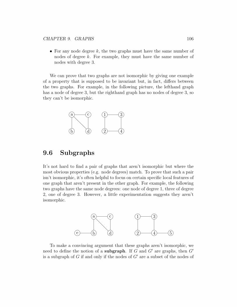
CHAPTER 9. GRAPHS 106
• For any node degree k, the two graphs must have the same number ofnodes of degree k. For example, they must have the same number ofnodes with degree 3.
We can prove that two graphs are not isomorphic by giving one exampleof a property that is supposed to be invariant but, in fact, differs betweenthe two graphs. For example, in the following picture, the lefthand graphhas a node of degree 3, but the righthand graph has no nodes of degree 3, sothey can’t be isomorphic.
a
b
c
d
1
2
3
4
9.6 Subgraphs
It’s not hard to find a pair of graphs that aren’t isomorphic but where themost obvious properties (e.g. node degrees) match. To prove that such a pairisn’t isomorphic, it’s often helpful to focus on certain specific local features ofone graph that aren’t present in the other graph. For example, the followingtwo graphs have the same node degrees: one node of degree 1, three of degree2, one of degree 3. However, a little experimentation suggests they aren’tisomorphic.
a
b
c
de
1
2
3
4 5
To make a convincing argument that these graphs aren’t isomorphic, weneed to define the notion of a subgraph. If G and G′ are graphs, then G′
is a subgraph of G if and only if the nodes of G′ are a subset of the nodes of
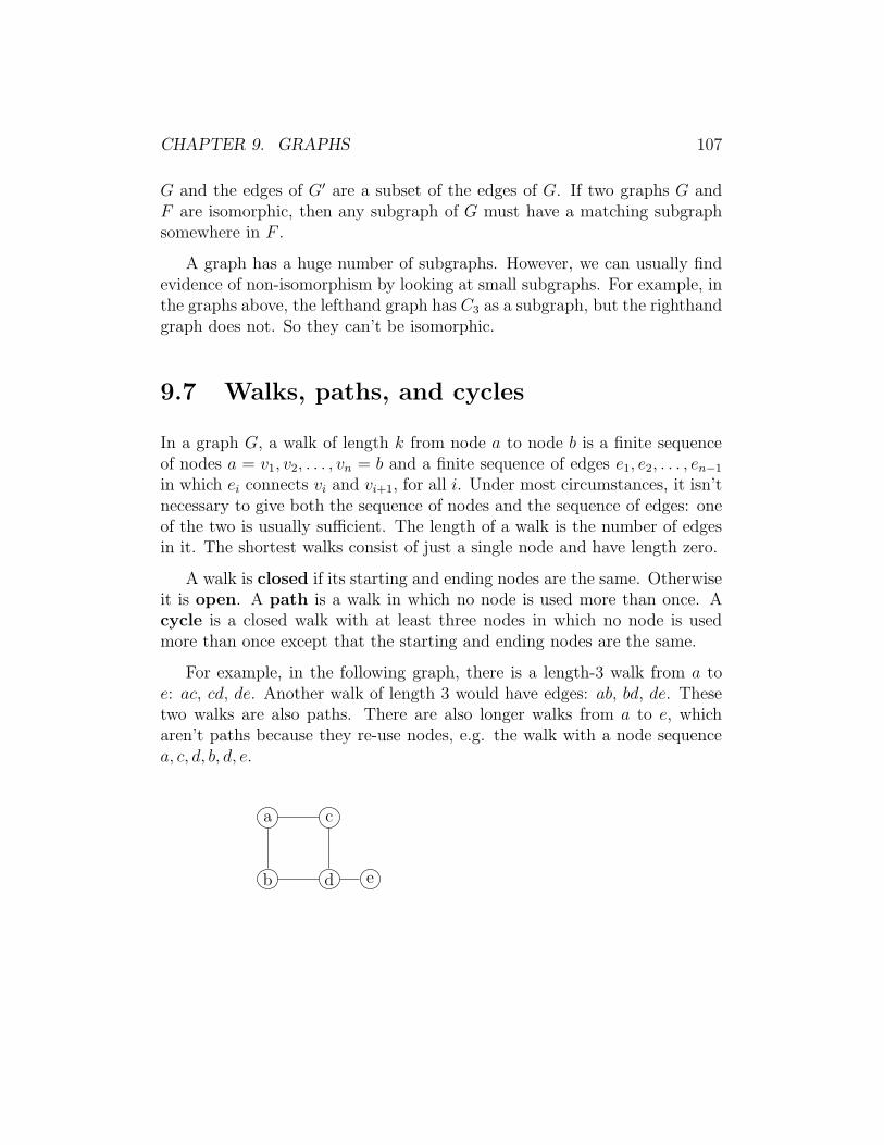
CHAPTER 9. GRAPHS 107
G and the edges of G′ are a subset of the edges of G. If two graphs G andF are isomorphic, then any subgraph of G must have a matching subgraphsomewhere in F .
A graph has a huge number of subgraphs. However, we can usually findevidence of non-isomorphism by looking at small subgraphs. For example, inthe graphs above, the lefthand graph has C3 as a subgraph, but the righthandgraph does not. So they can’t be isomorphic.
9.7 Walks, paths, and cycles
In a graph G, a walk of length k from node a to node b is a finite sequenceof nodes a = v1, v2, . . . , vn = b and a finite sequence of edges e1, e2, . . . , en−1
in which ei connects vi and vi+1, for all i. Under most circumstances, it isn’tnecessary to give both the sequence of nodes and the sequence of edges: oneof the two is usually sufficient. The length of a walk is the number of edgesin it. The shortest walks consist of just a single node and have length zero.
A walk is closed if its starting and ending nodes are the same. Otherwiseit is open. A path is a walk in which no node is used more than once. Acycle is a closed walk with at least three nodes in which no node is usedmore than once except that the starting and ending nodes are the same.
For example, in the following graph, there is a length-3 walk from a toe: ac, cd, de. Another walk of length 3 would have edges: ab, bd, de. Thesetwo walks are also paths. There are also longer walks from a to e, whicharen’t paths because they re-use nodes, e.g. the walk with a node sequencea, c, d, b, d, e.
a
b
c
d e

CHAPTER 9. GRAPHS 108
In the following graph, one cycle of length 4 has edges: ab, bc, ce, da.Other closely-related cycles go through the same nodes but with a differentstarting point or in the opposite direction, e.g. da, ab, bc, ce. Unlike cycles,closed walks can re-use nodes, e.g. ab, ba, ac, ce, ec, ca is a closed walk butnot a cycle.
a
b
c
d
e
f
The following graph is acyclic, i.e. it doesn’t contain any cycles.
a
b
c
d
e
f
Notice that the cycle graph Cn contains 2n different cycles. For example,if the vertices of C4 are labelled as shown below, then one cycle is ab, bc, cd, da,another is cd, bc, ab, da, and so forth.
ab
c d
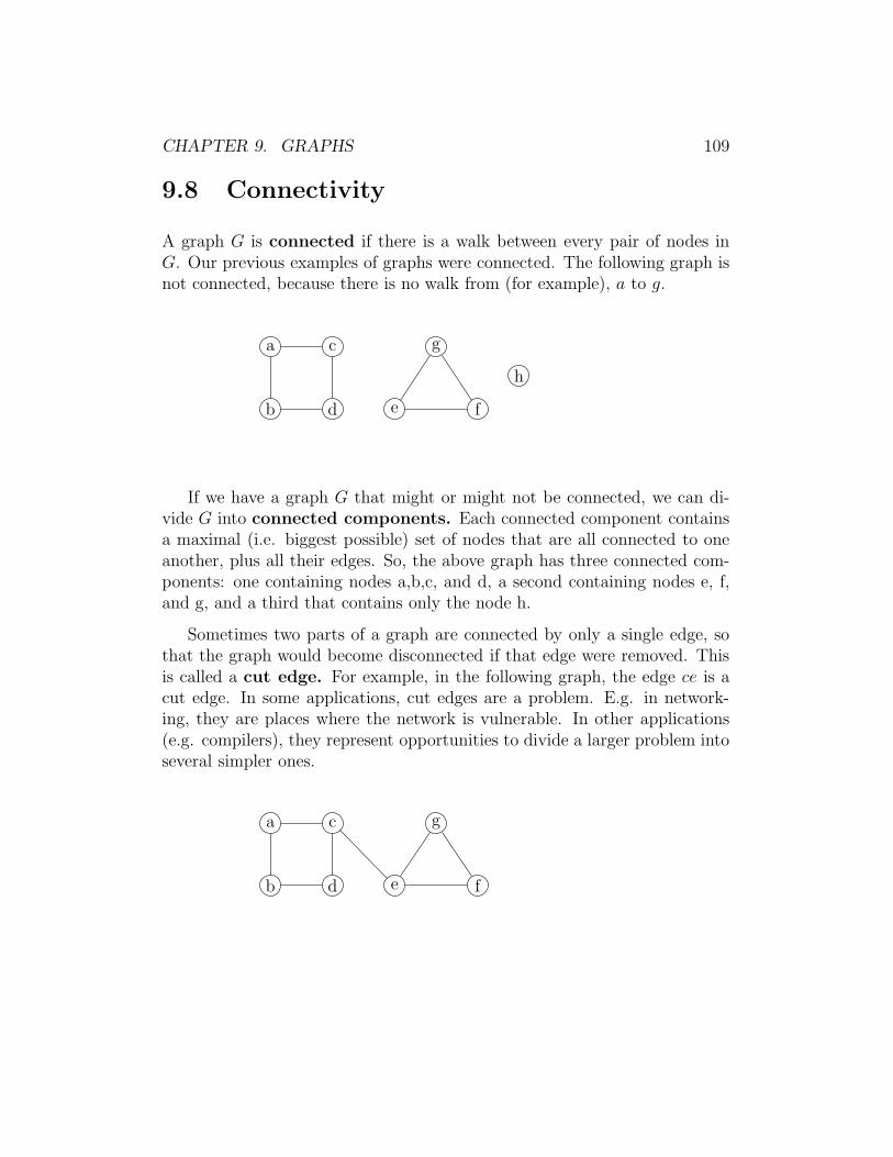
CHAPTER 9. GRAPHS 109
9.8 Connectivity
A graph G is connected if there is a walk between every pair of nodes inG. Our previous examples of graphs were connected. The following graph isnot connected, because there is no walk from (for example), a to g.
a
b
c
d e f
g
h
If we have a graph G that might or might not be connected, we can di-vide G into connected components. Each connected component containsa maximal (i.e. biggest possible) set of nodes that are all connected to oneanother, plus all their edges. So, the above graph has three connected com-ponents: one containing nodes a,b,c, and d, a second containing nodes e, f,and g, and a third that contains only the node h.
Sometimes two parts of a graph are connected by only a single edge, sothat the graph would become disconnected if that edge were removed. Thisis called a cut edge. For example, in the following graph, the edge ce is acut edge. In some applications, cut edges are a problem. E.g. in network-ing, they are places where the network is vulnerable. In other applications(e.g. compilers), they represent opportunities to divide a larger problem intoseveral simpler ones.
a
b
c
d e f
g

CHAPTER 9. GRAPHS 110
9.9 Distances
In graphs, distances are based on the lengths of paths connecting pairs ofnodes. Specifically, the distance d(a, b) between two nodes a and b is thelength of the shortest path from a to b. The diameter of a graph is themaximum distance between any pair of nodes in the graph. For example,the lefthand graph below has diameter 4, because d(f, e) = 4 and no otherpair of nodes is further apart. The righthand graph has diameter 2, becaused(1, 5) = 2 and no other pair of nodes is further apart.
f a
b
c
d e
1
2
3
4
5
9.10 Euler circuits
An Euler circuit of a graph G is a closed walk that uses each edge of thegraph exactly once. For example, one Euler circuit of the following graphwould be ac, cd, df , fe, ec, cf , fb, ba.
a
b
c
d
e
f
An Euler circuit is possible exactly when the graph is connected and eachnode has even degree. Each node has to have even degree because, in orderto complete the circuit, you have to leave each node that you enter. If the
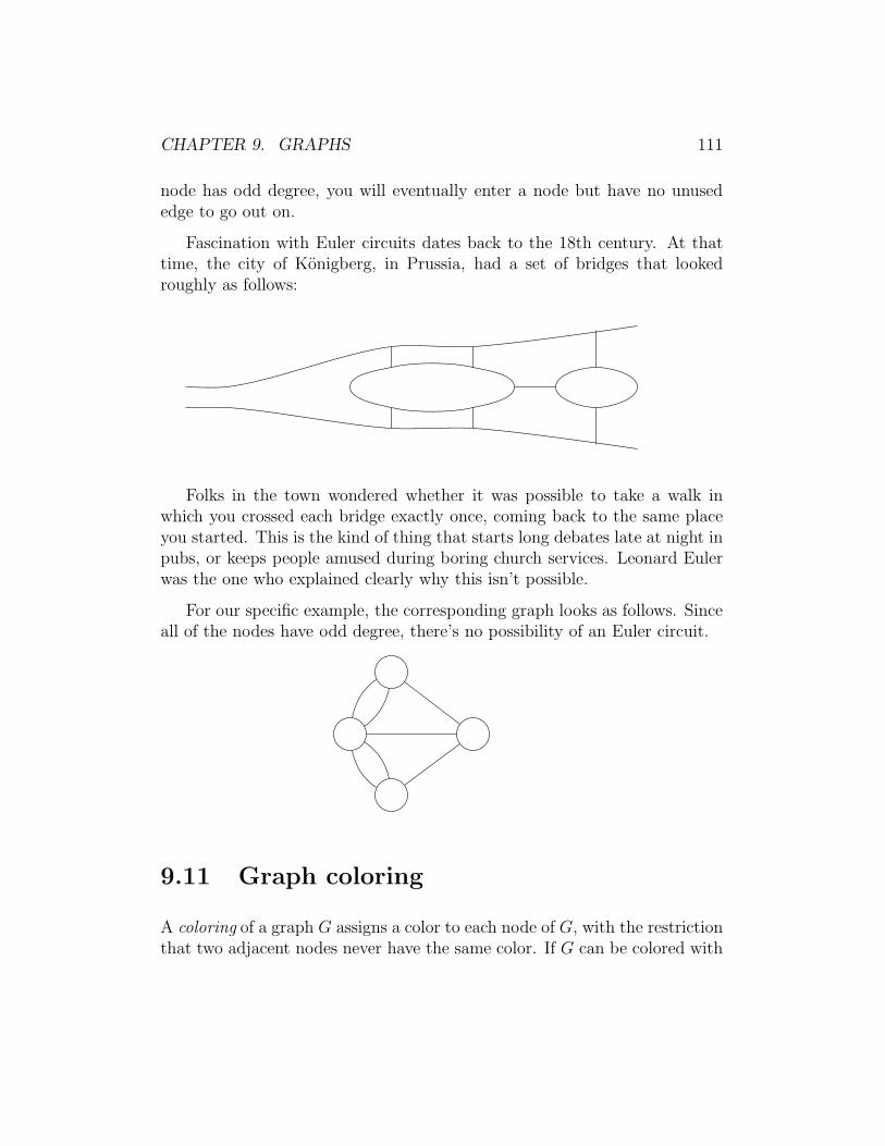
CHAPTER 9. GRAPHS 111
node has odd degree, you will eventually enter a node but have no unusededge to go out on.
Fascination with Euler circuits dates back to the 18th century. At thattime, the city of Konigberg, in Prussia, had a set of bridges that lookedroughly as follows:
Folks in the town wondered whether it was possible to take a walk inwhich you crossed each bridge exactly once, coming back to the same placeyou started. This is the kind of thing that starts long debates late at night inpubs, or keeps people amused during boring church services. Leonard Eulerwas the one who explained clearly why this isn’t possible.
For our specific example, the corresponding graph looks as follows. Sinceall of the nodes have odd degree, there’s no possibility of an Euler circuit.
9.11 Graph coloring
A coloring of a graph G assigns a color to each node of G, with the restrictionthat two adjacent nodes never have the same color. If G can be colored with

CHAPTER 9. GRAPHS 112
k colors, we say that G is k-colorable. The chromatic number of G, writtenχ(G), is the smallest number of colors needed to color G.
For example, only three colors are required for this graph:
R G
G B
R
But the complete graph Kn requires n colors, because each node is adja-cent to all the other nodes. E.g. K4 can be colored as follows:
R G
B Y
To establish that n is the chromatic number for a graph G, we need toestablish two facts:
• χ(G) ≤ n: G can be colored with n colors.
• χ(G) ≥ n: G cannot be colored with less than n colors
For small finite graphs, the simplest way to show that χ(G) ≤ n is to showa coloring of G that uses n colors.
Showing that χ(G) ≥ n can sometimes be equally straightforward. Forexample, G may contain a copy of Kn, which can’t be colored with less thann colors. However, sometimes it may be necessary to step carefully throughall the possible ways to color G with n−1 colors and show that none of themworks out.

CHAPTER 9. GRAPHS 113
So determining the chromatic number of a graph can be relatively easy forgraphs with a helpful structure, but quite difficult for other sorts of graphs.A fully general algorithm to find chromatic number will take time roughlyexponential in the size of the graph, for the most difficult input graphs.1 Sucha slow running time isn’t practical except for small examples, so applicationstend to focus on approximate solutions.
9.12 Why should I care?
Graph coloring is required for solving a wide range of practical problems. Forexample, there is a coloring algorithm embedded in most compilers. Becausethe general problem can’t be solved efficiently, the implemented algorithmsuse limitations or approximations of various sorts so that they can run in areasonable amount of time.
For example, suppose that we want to allocate broadcast frequencies tolocal radio stations. In the corresponding graph problem, each station is anode and the frequencies are the “colors.” Two stations are connected byan edge if they are geographically too close together, so that they wouldinterfere if they used the same frequency. This graph should not be too badto color in practice, so long as we have a large enough supply of frequenciescompared to the numbers of stations clustered near one another.
We can model a sudoku puzzle by setting up one node for each square.The colors are the 9 numbers, and some are pre-assigned to certain nodes.Two nodes are connected if their squares are in the same block or row orcolumn. The puzzle is solvable if we can 9-color this graph, respecting thepre-assigned colors.
We can model exam scheduling as a coloring problem. The exams for twocourses should not be put at the same time if there is a student who is inboth courses. So we can model this as a graph, in which each course is a nodeand courses are connected by edges if they share students. The question isthen whether we can color the graph with k colors, where k is the number ofexam times in our schedule.
In the exam scheduling problem, we actually expect the answer to be
1In CS theory jargon, this problem is “HP-hard.”
CHAPTER 9. GRAPHS 114
“no,” because eliminating conflicts would require an excessive number ofexam times. So the real practical problem is: how few students do we haveto take out of the picture (i.e. give special conflict exams to) in order to beable to solve the coloring problem with a reasonable value for k. We alsohave the option of splitting a course (i.e. offering a scheduled conflict exam)to simplify the graph.
A particularly important use of coloring in computer science is registerallocation. A large java or C program contains many named variables. Buta computer has a smallish number (e.g. 32) of fast registers which can feedbasic operations such as addition. So variables must be allocated to specificregisters.
The nodes in this coloring problem are variables. The colors are registers.Two variables are connected by an edge if they are in use at the same timeand, therefore, cannot share a register. As with the exam scheduling problem,we actually expect the raw coloring problem to fail. The compiler then usesso-called “spill” operations to break up the dependencies and create a graphwe can color with our limited number of registers. The goal is to use as fewspills as possible.
9.13 Bipartite graphs
Another special type of graph is a bipartite graph. A graph G = (V,E)is bipartite if we can split V into two non-overlapping subsets V1 and V2
such that every edge in G connects an element of V1 with an element of V2.That is, no edge connects two nodes from the same part of the division. Or,alternatively, a graph is bipartite if and only if it is 2-colorable.
For example, the cube graph is bipartite because we can color it with twocolors:
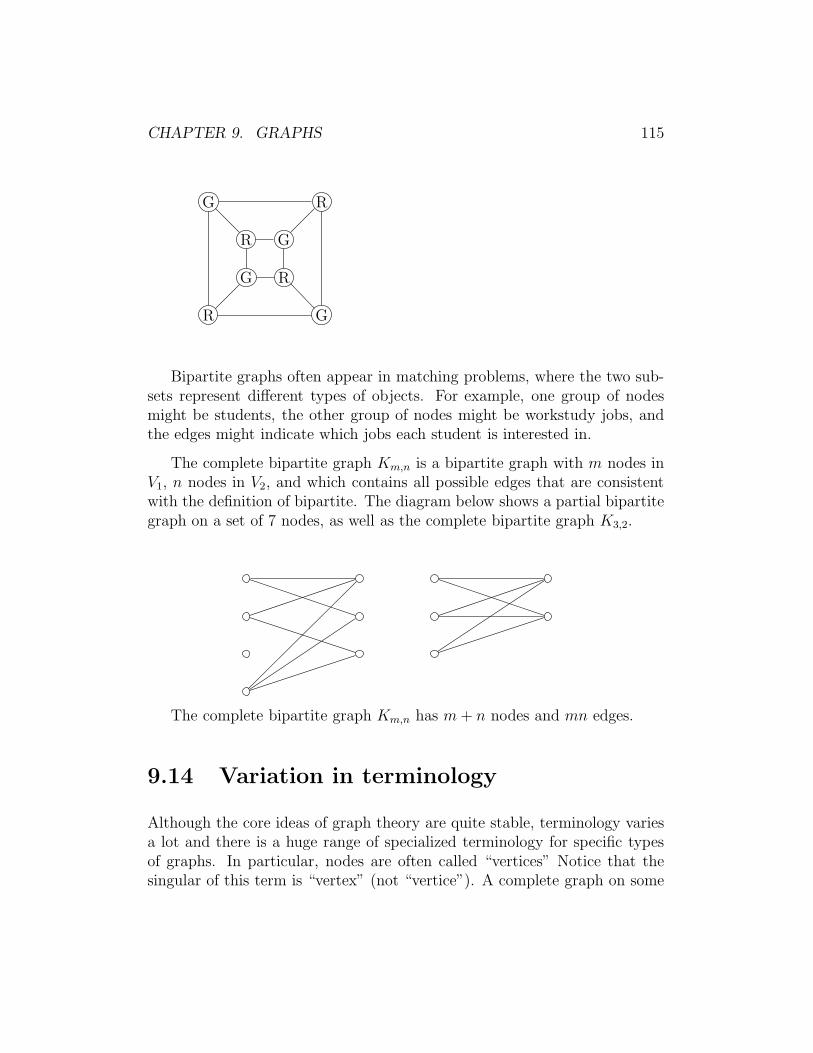
CHAPTER 9. GRAPHS 115
R
RG
G
G
GR
R
Bipartite graphs often appear in matching problems, where the two sub-sets represent different types of objects. For example, one group of nodesmight be students, the other group of nodes might be workstudy jobs, andthe edges might indicate which jobs each student is interested in.
The complete bipartite graph Km,n is a bipartite graph with m nodes inV1, n nodes in V2, and which contains all possible edges that are consistentwith the definition of bipartite. The diagram below shows a partial bipartitegraph on a set of 7 nodes, as well as the complete bipartite graph K3,2.
The complete bipartite graph Km,n has m+ n nodes and mn edges.
9.14 Variation in terminology
Although the core ideas of graph theory are quite stable, terminology variesa lot and there is a huge range of specialized terminology for specific typesof graphs. In particular, nodes are often called “vertices” Notice that thesingular of this term is “vertex” (not “vertice”). A complete graph on some
CHAPTER 9. GRAPHS 116
set of vertices is also known as a clique.
What we’re calling a “walk” used to be widely called a “path.” Authorswho still use this convention would then use the term “simple path” to ex-clude repetition of vertices. Terms for closely-related concepts, e.g. cycle,often change as well.

Chapter 10
Induction
This chapter covers mathematical induction.
10.1 Introduction to induction
At the start of the term, we saw the following formula for computing thesum of the first n integers:
Claim 38 For any positive integer n, Σni=1 i = n(n+1)
2.
At that point, we didn’t prove this formula correct, because this is mosteasily done using a new proof technique: induction.
Mathematical induction is a technique for showing that a statement P (n)is true for all natural numbers n, or for some infinite subset of the naturalnumbers (e.g. all positive even integers). It’s a nice way to produce quick,easy-to-read proofs for a variety of fact that would be awkward to prove withthe techniques you’ve seen so far. It is particularly well suited to analyzingthe performance of recursive algorithms. Most of you have seen a few of thesein previous programming classes; you’ll see many more in later classes.
Induction is very handy, but it may strike you as a bit weird. It maytake you some time to get used to it. In fact, you have two tasks which aresomewhat independent:
117
CHAPTER 10. INDUCTION 118
• Learn how to write an inductive proof.
• Understand why inductive proofs are legitimate.
You can learn to write correct inductive proofs even if you remain some-what unsure of why the method is legitimate. Over the next few classes,you’ll gain confidence in the validity of induction and its friend recursion.
10.2 An Example
A proof by induction has the following outline:
Claim: P (n) is true for all positive integers n.
Proof: We’ll use induction on n.
Base: We need to show that P (1) is true.
Induction: Suppose that P (n) is true for n = 1, 2, . . . , k−1. Weneed to show that P (k) is true.
The part of the proof labelled “induction” is a conditional statement. Weassume that P (n) is true for values of n no larger than k−1. This assumptionis called the inductive hypothesis. We use this assumption to show that P (k)is true.
For our formula example, our proposition P (n) is Σni=1 i = n(n+1)
2. Sub-
stituting this definition of P into the outline, we get the following outline forour specific claim:
Proof: We will show that Σni=1 i =
n(n+1)2
for any positive integern, using induction on n.
Base: We need to show that the formula holds for n = 1, i.e.Σ1
i=1 i = 1·22.
Induction: Suppose that Σni=1 i = n(n+1)
2for n = 1, 2, . . . , k − 1.
We need to show that Σki=1 i = k(k+1)
2.
CHAPTER 10. INDUCTION 119
The full proof might then look like:
Proof: We will show that Σni=1 i =
n(n+1)2
for any positive integern, using induction on n.
Base: We need to show that the formula holds for n = 1. Σ1i=1 i =
1. And also 1·22
= 1. So the two are equal for n = 1.
Induction: Suppose that Σni=1 i = n(n+1)
2for n = 1, 2, . . . , k − 1.
We need to show that Σki=1 i = k(k+1)
2.
By the definition of summation notation, Σki=1 i = (Σk−1
i=1 i) + k
Our inductive hypothesis states that at n = k − 1, Σ−1i=1k i =
( (k−1)k2
).
Combining these two formulas, we get that Σki=1 i = ( (k−1)k
2) + k.
But ( (k−1)k2
) + k = ( (k−1)k2
) + 2k2= ( (k−1+2)k
2) = k(k+1)
2.
So, combining these equations, we get that Σki=1 i =
k(k+1)2
whichis what we needed to show.
One way to think of a proof by induction is that it’s a template forbuilding direct proofs. If I give you the specific value n = 47, you couldwrite a direct proof by starting with the base case and using the inductivestep 46 times to work your way from the n = 1 case up to the n = 47 case.
10.3 Why is this legit?
There are several ways to think about mathematical induction, and under-stand why it’s a legitimate proof technique. Different people prefer differentmotivations at this point, so I’ll offer several.
Domino Theory: Imagine an infinite line of dominoes. Thebase step pushes the first one over. The inductive step claimsthat one domino falling down will push over the next dominoin the line. So dominos will start to fall from the beginning allthe way down the line. This process continues forever, because

CHAPTER 10. INDUCTION 120
the line is infinitely long. However, if you focus on any specificdomino, it falls after some specific finite delay.
Recursion fairy: The recursion fairy is the mathematician’sversion of a programming assistant. Suppose you tell her how todo the proof for P (1) and also why P (1) up through P (k) impliesP (k + 1). Then suppose you pick any integer (e.g. 1034) thenshe can take this recipe and use it to fill in all the details of anormal direct proof that P holds for this particular integer. Thatis, she takes P (1), then uses the inductive step to get from P (1)to P (2), and so on up to P (1034).
Smallest counter-example: Let’s assume we’ve establishedthat P (1) is true. Suppose also that (*) if P (n) is true forn = 1, . . . , k − 1 then P (k) is true. Let’s prove that P (j) istrue for all positive integers j, by contradiction.
That is, we suppose that P (1) is true and (*) is true but there isa counter-example to our claim that P (j) is true for all j. Thatis, suppose that P (m) was not true for some integer m.
Now, let’s look at the set of all counter-examples. We know thatall the counter-examples are larger than 1, because our inductionproof established explicitly that P (1) was true. Suppose that thesmallest counter-example is s. So P (s) is not true. We knowthat s > 1, since P (1) was true. Since s was supposed to be thesmallest counter-example, then none of 1, 2, . . . , s − 1 can be acounter-example, i.e. P (n) is true for all these smaller values ofn. So, by (*), we know that P (s) is true.
But now we have a contradiction, because we’ve shown that P (s)is both true and false.
The smallest counter-example explanation is a formal proof that inductionworks, given how we’ve defined the integers. If you dig into the mathematics,you’ll find that it depends on the integers having what’s called the “well-ordering” property: any subset that has a lower bound also has a smallestelement. Standard axioms used to define the integers include either a well-ordering or an induction axiom.

CHAPTER 10. INDUCTION 121
These arguments don’t depend on whether our starting point is 1 or someother integer, e.g. 0 or 2 or -47. All you need to do is ensure that your basecase covers the first integer for which the claim is supposed to be true.
10.4 Building an inductive proof
In constructing an inductive proof, you’ve got two tasks. First, you needto set up this outline for your problem. This includes identifying a suitableproposition P and a suitable integer variable n.
Notice that P (n) must be a statement, i.e. something that is either trueor false. For example, it is never just a formula whose value is a number.Also, notice that P (n) must depend on an integer n. This integer n is knownas our induction variable. The assumption at the start of the inductive step(“P (k) is true”) is called the inductive hypothesis.
Your second task is to fill in the middle part of the induction step. Thatis, you must figure out how to relate a solution for a larger problem P (k) toa solution for one or more of the smaller problems P (1) . . . , P (k − 1). Moststudents want to do this by starting with a small problem, e.g. P (k−1), andadding something to it. For more complex situations, however, it’s usuallybetter to start with the larger problem and try to find an instance of thesmaller problem inside it.
10.5 Another example of induction
Let’s do another example:
Claim 39 For every positive integer n ≥ 4, 2n < n!.
First, you should try (on your own) some specific integers and verify thatthe claim is true. Since the claim specifies n ≥ 4, it’s worth checking that 4does work but the smaller integers don’t.
In this claim, the proposition P (n) is 2n < n!. So an outline of ourinductive proof looks like:

CHAPTER 10. INDUCTION 122
Proof: Suppose that n is an integer and n ≥ 4. We’ll prove that2n < n! using induction on n.
Base: n = 4. [show that the formula works for n = 4]
Induction: Suppose that 2n < n! holds for n = 4, 5, . . . , k. Thatis, suppose that we have an integer k ≥ 4 such that 2k < k!.We need to show that the claim holds for n = k + 1, i.e. that2k+1 < (k + 1)!.
Notice that our base case is for n = 4 because the claim was specifiedto hold only for integers ≥ 4. We’ve also used a variation on our inductionoutline, where the induction hypothesis covers values up through k (insteadof k − 1) and we prove the claim at n = k + 1 (instead of at n = k). Itdoesn’t matter whether your hypothesis goes through n = k− 1 or n = k, aslong as you prove the claim for the next larger integer.
Fleshing out the details of the algebra, we get the following full proof.When working with inequalities, it’s especially important to write down yourassumptions and what you want to conclude with. You can then work fromboth ends to fill in the gap in the middle of the proof.
Proof: Suppose that n is an integer and n ≥ 4. We’ll prove that2n < n! using induction on n.
Base: n = 4. In this case 2n = 24 = 16. Also n! = 1 · 2 · 3 · 4 = 24.Since 16 < 24, the formula holds for n = 4.
Induction: Suppose that 2n < n! holds for n = 4, 5, . . . , k. Thatis, suppose that we have an integer k ≥ 4 such that 2k < k!. Weneed to show that 2k+1 < (k + 1)!.
2k+1 = 2·2k. By the inductive hypothesis, 2k < k!, so 2·2k < 2·k!.Since k ≥ 4, 2 < k + 1. So 2 · k! < (k + 1) · k! = (k + 1)!.
Putting these equations together, we find that 2k+1 < (k + 1)!,which is what we needed to show.

CHAPTER 10. INDUCTION 123
10.6 Some comments about style
Notice that the start of the proof tells you which variable in your formula (nin this case) is the induction variable. In this formula, the choice of induc-tion variable is fairly obvious. But sometimes there’s more than one integerfloating around that might make a plausible choice for the induction variable.It’s good style to always mention that you are doing a proof by induction,say what your induction variable is, and label your base and inductive steps.
Notice that the proof of the base case is very short. In fact, I’ve writtenabout about twice as long as you’d normally see it. Almost all the time, thebase case is trivial to prove and fairly obvious to both you and your reader.Often this step contains only some worked algebra and a check mark at theend. However, it’s critical that you do check the base case. And, if your basecase involves an equation, compute the results for both sides (not just oneside) so you can verify they are equal.
The important part of the inductive step is ensuring that you assumeP (1), . . . , P (k− 1) and use these facts to show P (k). At the start, you mustspell out your inductive hypothesis, i.e. what P (n) is for your claim. It’susually helpful to explicitly substitute in some key values for n, e.g. work outwhat P (k−1) is. Make sure that you use the information from the inductivehypothesis in your argument that P (k + 1) holds. If you don’t, it’s not aninductive proof and it’s very likely that your proof is buggy.
At the start of the inductive step, it’s also a good idea to say what youneed to show, i.e. quote what P (k) is.
These “style” issues are optional in theory, but actually critical for be-ginners writing inductive proofs. You will lose points if your proof isn’t clearand easy to read. Following these style points (e.g. labelling your base andinductive steps) is a good way to ensure that it is, and that the logic of yourproof is correct.
10.7 Another example
The previous examples applied induction to an algebraic formula. We canalso apply induction to other sorts of statements, as long as they involve a
CHAPTER 10. INDUCTION 124
suitable integer n.
Claim 40 For any natural number n, n3 − n is divisible by 3.
In this case, P (n) is “n3 − n is divisible by 3.”
Proof: By induction on n.
Base: Let n = 0. Then n3 − n = 03 − 0 = 0 which is divisible by3.
Induction: Suppose that n3−n is divisible by 3, for n = 0, 1, . . . , k.We need to show that (k + 1)3 − (k + 1) is divisible by 3.
(k+1)3−(k+1) = (k3+3k2+3k+1)−(k+1) = (k3−k)+3(k2+k)
From the inductive hypothesis, (k3 − k) is divisible by 3. And3(k2 + k) is divisible by 3 since (k2 + k) is an integer. So theirsum is divisible by 3. That is (k + 1)3 − (k + 1) is divisible by 3.�
The zero base case is technically enough to make the proof solid, butsometimes a zero base case doesn’t provide good intuition or confidence. Soyou’ll sometimes see an extra base case written out, e.g. n = 1 in thisexample, to help the author or reader see why the claim is plausible.
10.8 A geometrical example
Let’s see another example of the basic induction outline, this time on ageometrical application. Tiling some area of space with a certain type ofpuzzle piece means that you fit the puzzle pieces onto that area of spaceexactly, with no overlaps or missing areas. A right triomino is a 2-by-2square minus one of the four squares.

CHAPTER 10. INDUCTION 125
I claim that
Claim 41 For any positive integer n, a 2n × 2n checkerboard with any onesquare removed can be tiled using right triominoes.
Proof: by induction on n.
Base: Suppose n = 1. Then our 2n × 2n checkerboard with onesquare removed is exactly one right triomino.
Induction: Suppose that the claim is true for n = 1, . . . , k. Thatis a 2n × 2n checkerboard with any one square removed can betiled using right triominoes as long as n ≤ k.
Suppose we have a 2k+1 × 2k+1 checkerboard C with any onesquare removed. We can divide C into four 2k×2k sub-checkerboardsP , Q, R, and S. One of these sub-checkerboards is already miss-ing a square. Suppose without loss of generality that this one isS. Place a single right triomino in the middle of C so it coversone square on each of P , Q, and R.
Now look at the areas remaining to be covered. In each of thesub-checkerboards, exactly one square is missing (S) or alreadycovered (P , Q, and R). So, by our inductive hypothesis, eachof these sub-checkerboards minus one square can be tiled withright triominoes. Combining these four tilings with the triominowe put in the middle, we get a tiling for the whole of the largercheckerboard C. This is what we needed to construct.

CHAPTER 10. INDUCTION 126
10.9 Graph coloring
We can also use induction to prove a useful general fact about graph col-orability:
Claim 42 If all nodes in a graph G have degree ≤ D, then G can be coloredwith D + 1 colors.
The objects involved in this claim are graphs. To apply induction toobjects like graphs, we organize our objects by their size. Each step in theinduction process will show that the claim holds for all objects of a particular(integer) size. For graphs, the “size” would typically be either the numberof nodes or the number of edges. For this proof, it’s most convenient to usethe number of nodes.
Proof: by induction on the number of nodes in G.
Base: The graph with just one node has maximum degree 0 andcan be colored with one color.
Induction: Suppose that any graph with at most k−1 nodes andmaximum node degree ≤ D can be colored with D + 1 colors.
Let G be a graph with k nodes and maximum node degree D.Remove some node v (and its edges) from G to create a smallergraph G′.
G′ has k − 1 nodes. Also, the maximum node degree of G′ isno larger than D, because removing a node can’t increase thedegree. So, by the inductive hypothesis, G′ can be colored withD + 1 colors.
Because v has at most D neighbors, its neighbors are only usingD of the available colors, leaving a spare color that we can assignto v. The coloring of G′ can be extended to a coloring of G withD + 1 colors.
We can use this idea to design an algorithm (called the “greedy” algo-rithm) for coloring a graph. This algorithm walks through the nodes one-by-one, giving each node a color without revising any of the previously-assigned
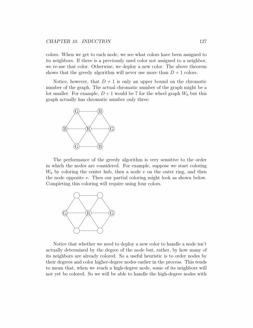
CHAPTER 10. INDUCTION 127
colors. When we get to each node, we see what colors have been assigned toits neighbors. If there is a previously used color not assigned to a neighbor,we re-use that color. Otherwise, we deploy a new color. The above theoremshows that the greedy algorithm will never use more than D + 1 colors.
Notice, however, that D + 1 is only an upper bound on the chromaticnumber of the graph. The actual chromatic number of the graph might be alot smaller. For example, D + 1 would be 7 for the wheel graph W6 but thisgraph actually has chromatic number only three:
G B
G B
B GR
The performance of the greedy algorithm is very sensitive to the orderin which the nodes are considered. For example, suppose we start coloringW6 by coloring the center hub, then a node v on the outer ring, and thenthe node opposite v. Then our partial coloring might look as shown below.Completing this coloring will require using four colors.
G GR
Notice that whether we need to deploy a new color to handle a node isn’tactually determined by the degree of the node but, rather, by how many ofits neighbors are already colored. So a useful heuristic is to order nodes bytheir degrees and color higher-degree nodes earlier in the process. This tendsto mean that, when we reach a high-degree node, some of its neighbors willnot yet be colored. So we will be able to handle the high-degree nodes with
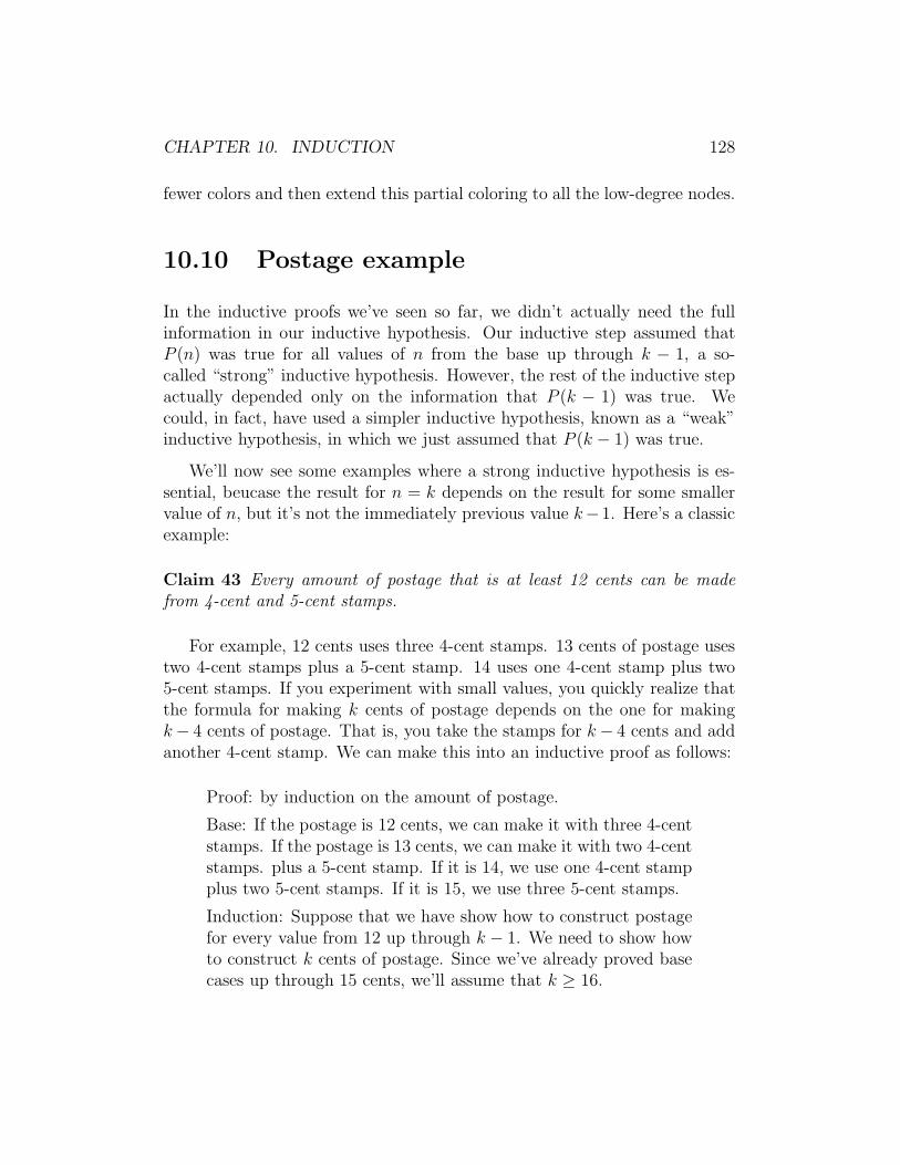
CHAPTER 10. INDUCTION 128
fewer colors and then extend this partial coloring to all the low-degree nodes.
10.10 Postage example
In the inductive proofs we’ve seen so far, we didn’t actually need the fullinformation in our inductive hypothesis. Our inductive step assumed thatP (n) was true for all values of n from the base up through k − 1, a so-called “strong” inductive hypothesis. However, the rest of the inductive stepactually depended only on the information that P (k − 1) was true. Wecould, in fact, have used a simpler inductive hypothesis, known as a “weak”inductive hypothesis, in which we just assumed that P (k − 1) was true.
We’ll now see some examples where a strong inductive hypothesis is es-sential, beucase the result for n = k depends on the result for some smallervalue of n, but it’s not the immediately previous value k−1. Here’s a classicexample:
Claim 43 Every amount of postage that is at least 12 cents can be madefrom 4-cent and 5-cent stamps.
For example, 12 cents uses three 4-cent stamps. 13 cents of postage usestwo 4-cent stamps plus a 5-cent stamp. 14 uses one 4-cent stamp plus two5-cent stamps. If you experiment with small values, you quickly realize thatthe formula for making k cents of postage depends on the one for makingk− 4 cents of postage. That is, you take the stamps for k− 4 cents and addanother 4-cent stamp. We can make this into an inductive proof as follows:
Proof: by induction on the amount of postage.
Base: If the postage is 12 cents, we can make it with three 4-centstamps. If the postage is 13 cents, we can make it with two 4-centstamps. plus a 5-cent stamp. If it is 14, we use one 4-cent stampplus two 5-cent stamps. If it is 15, we use three 5-cent stamps.
Induction: Suppose that we have show how to construct postagefor every value from 12 up through k − 1. We need to show howto construct k cents of postage. Since we’ve already proved basecases up through 15 cents, we’ll assume that k ≥ 16.

CHAPTER 10. INDUCTION 129
Since k ≥ 16, k − 4 ≥ 12. So by the inductive hypothesis, wecan construct postage for k− 4 cents using m 4-cent stamps andn 5-cent stamps, for some natural numbers m and n. In otherwords k − 4 = 4m+ 5n.
But then k = 4(m + 1) + 5n. So we can construct k cents ofpostage using m+1 4-cent stamps and n 5-cent stamps, which iswhat we needed to show.
Notice that we needed to directly prove four base cases, since we neededto reach back four integers in our inductive step. It’s not always obvious howmany base cases are needed until you work out the details of your inductivestep.
10.11 Nim
In the parlour game Nim, there are two players and two piles of matches. Ateach turn, a player removes some (non-zero) number of matches from one ofthe piles. The player who removes the last match wins.1
Claim 44 If the two piles contain the same number of matches at the startof the game, then the second player can always win.
Here’s a winning strategy for the second player. Suppose your opponentremoves m matches from one pile. In your next move, you remove m matchesfrom the other pile, thus evening up the piles. Let’s prove that this strategyworks.
Proof by induction on the number of matches (n) in each pile.
Base: If both piles contain 1 match, the first player has only onepossible move: remove the last match from one pile. The secondplayer can then remove the last match from the other pile andthereby win.
1Or, in some variations, loses. There seem to be several variations of this game.

CHAPTER 10. INDUCTION 130
Induction: Suppose that the second player can win any game thatstarts with two piles of n matches, where n is any value from 1through k − 1. We need to show that this is true if n = k.
So, suppose that both piles contain k matches. A legal move bythe first player involves removing j matches from one pile, where1 ≤ j ≤ k. The piles then contain k matches and k − j matches.
The second player can now remove j matches from the other pile.This leaves us with two piles of k − j matches. If j = k, thenthe second player wins. If j < k, then we’re now effectively atthe start of a game with k − j matches in each pile. Since j ≥ 1,k− j ≤ k− 1. So, by the induction hypothesis, we know that thesecond player can finish the rest of the game with a win.
The induction step in this proof uses the fact that our claim P (n) istrue for a smaller value of n. But since we can’t control how many matchesthe first player removes, we don’t know how far back we have look in thesequence of earlier results P (1) . . . P (k). Our previous proof about postagecan be rewritten so as to avoid strong induction. It’s less clear how to rewriteproofs like this Nim example.
10.12 Prime factorization
Early in this course, we saw the “Fundamental Theorem of Arithmetic,”which states that every positive integer n, n ≥ 2, can be expressed as theproduct of one or more prime numbers. Let’s prove that this is true.
Recall that a number n is prime if its only positive factors are one andn. n is composite if it’s not prime. Since a factor of a number must be nolarger than the number itself, this means that a composite number n alwayshas a factor larger than 1 but smaller than n. This, in turn, means that wecan write n as ab, where a and b are both larger than 1 but smaller than n.2
Proof by induction on n.
2We’ll leave the details of proving this as an exercise for the reader.
CHAPTER 10. INDUCTION 131
Base: 2 can be written as the product of a single prime number,2.
Induction: Suppose that every integer between 2 and k can bewritten as the product of one or more primes. We need to showthat k + 1 can be written as a product of primes. There are twocases:
Case 1: k + 1 is prime. Then it is the product of one prime, i.e.itself.
Case 2: k + 1 is composite. Then k + 1 can be written as ab,where a and b are integers such that a and b lie in the range[2, k]. By the induction hypothesis, a can be written as a productof primes p1p2 . . . pi and b can be written as a product of primesq1q2 . . . qj . So then k+1 can be written as the product of primesp1p2 . . . piq1q2 . . . qj .
In both cases k+ 1 can be written as a product of primes, whichis what we needed to show.
Again, the inductive step needed to reach back some number of steps inour sequence of results, but we couldn’t control how far back we needed togo.
10.13 Variation in notation
Certain details of the induction outline vary, depending on the individualpreferences of the author and the specific claim being proved. Some folksprefer to assume the statement is true for k and prove it’s true for k + 1.Other assume it’s true for k − 1 and prove it’s true for k. For a specificproblems, sometimes one or the other choice yields a slightly simpler proofs.
Some authors prefer to write strong induction hypotheses all the time,even when a weak hypothesis would be sufficient. This saves mental effort,because you don’t have to figure out in advance whether a strong hypothesiswas really required. However, for some problems, a strong hypothesis maybe more complicated to state than a weak one.
CHAPTER 10. INDUCTION 132
Authors writing for more experienced audiences may abbreviate the out-line somewhat, e.g. packing an entirely short proof into one paragraph with-out labelling the base and inductive steps separately. However, being carefulabout the outline is important when you are still getting used to the tech-nique.

Chapter 11
Recursive Definition
This chapter covers recursive definition, including finding closed forms.
11.1 Recursive definitions
Thus far, we have defined objects of variable length using semi-formal defi-nitions involving . . .. For example, we defined the summation
∑n
i=1 i by
n∑
i=1
i = 1 + 2 + 3 + . . .+ (n− 1) + n
This method is only ok when the reader can easily see what regular patternthe . . . is trying to express. When precision is essential, e.g. when the patternis less obvious, we need to switch to “recursive definitions.”
Recursive function definitions in mathematics are basically similar to re-cursive procedures in programming languages. A recursive definition definesan object in terms of smaller objects of the same type. Because this pro-cess has to end at some point, we need to include explicit definitions for thesmallest objects. So a recursive definition always has two parts:
• Base case or cases
133
CHAPTER 11. RECURSIVE DEFINITION 134
• Recursive formula
For example, the summation∑n
i=1 i can be defined as:
• g(1) = 1
• g(n) = g(n− 1) + n, for all n ≥ 2
Both the base case and the recursive formula must be present to have acomplete definition. However, it is traditional not to explicitly label these twopieces. You’re just expected to figure out for yourself which parts are basecase(s) and which is the recursive formula. The input values are normallyassumed to be integers.
The true power of recursive definition is revealed when the result forn depends on the results for more than one smaller value, as in the stronginduction examples. For example, the famous Fibonacci numbers are defined:
• F0 = 0
• F1 = 1
• Fi = Fi−1 + Fi−2, ∀i ≥ 2
So F2 = 1, F3 = 2, F4 = 3, F5 = 5, F6 = 8, F7 = 13, F8 = 21, F9 = 34. Itisn’t at all obvious how to express this pattern non-recursively.
11.2 Finding closed forms
Many recursive numerical formulas have a closed form, i.e. an equivalentexpression that doesn’t involve recursion (or summation or the like). Some-times you can find the closed form by working out the first few values ofthe function and then guessing the pattern. More often, you need to usean organized technique. The simplest technique for finding closed forms iscalled “unrolling.”
For example, suppose we have a function T : N → Z defined by

CHAPTER 11. RECURSIVE DEFINITION 135
T (1) = 1
T (n) = 2T (n− 1) + 3, ∀n ≥ 2
The values of this function are T (1) = 1, T (2) = 5, T (3) = 13, T (4) = 29,T (5) = 61. It isn’t so obvious what the pattern is.
The idea behind unrolling is to substitute a recursive definition into itself,so as to re-express T (n) in terms of T (n− 2) rather than T (n− 1). We keepdoing this, expressing T (n) in terms of the value of T for smaller and smallerinputs, until we can see the pattern required to express T (n) in terms of nand T (0). So, for our example function, we would compute:
T (n) = 2T (n− 1) + 3
= 2(2T (n− 2) + 3) + 3
= 2(2(2T (n− 3) + 3) + 3) + 3
= 23T (n− 3) + 22 · 3 + 2 · 3 + 3
= 24T (n− 4) + 23 · 3 + 22 · 3 + 2 · 3 + 3
. . .
= 2kT (n− k) + 2k−1 · 3 + . . .+ 22 · 3 + 2 · 3 + 3
The first few lines of this are mechanical substitution. To get to the last line,you have to imagine what the pattern looks like after k substitutions.
We can use summation notation to compactly represent the result of thekth unrolling step:
T (n) = 2kT (n− k) + 2k−1 · 3 + . . .+ 22 · 3 + 2 · 3 + 3
= 2kT (n− k) + 3(2k−1 + . . .+ 22 + 2 + 1)
= 2kT (n− k) + 3
k−1∑
i=0
(2i)
CHAPTER 11. RECURSIVE DEFINITION 136
Now, we need to determine when the input to T will hit the base case. Inour example, the input value is n− k and the base case is for an input of 1.So we hit the base case when n − k = 1. i.e. when k = n − 1. Substitutingthis value for k back into our equation, and using the fact that T (1) = 1, weget
T (n) = 2kT (n− k) + 3
k−1∑
i=0
(2i)
= 2n−1T (1) + 3
n−2∑
i=0
(2i)
= 2n−1 + 3n−2∑
k=0
(2k)
= 2n−1 + 3(2n−1 − 1) = 4(2n−1)− 3 = 2n+1 − 3
So the closed form for this function is T (n) = 2n+1 − 3. The unrollingprocess isn’t a formal proof that our closed form is correct. However, we’llsee below how to write a formal proof using induction.
11.3 Divide and conquer
Many important algorithms in computer science involve dividing a big prob-lem of (integer) size n into a sub-problems, each of size n/b. This generalmethod is called “divide and conquer.” Analyzing such algorithms involvesrecursive definitions that look like:
S(1) = c
S(n) = aS(⌈n/b⌉) + f(n), ∀n ≥ 2
The base case takes some constant amount of work c. The term f(n) isthe work involved in dividing up the big problem and/or merging together
CHAPTER 11. RECURSIVE DEFINITION 137
the solutions for the smaller problems. The call to the ceiling function isrequired to ensure that the input to S is always an integer.
Handling such definitions in full generality is beyond the scope of thisclass.1 So let’s consider a particularly important special case: dividing ourproblem into two half-size problems, where the dividing/merging takes timeproportional to the size of the problem. And let’s also restrict our input nto be a power of two, so that we don’t need to use the ceiling function. Wethen get a recursive definition that looks like:
S(1) = c
S(n) = 2S(n/2) + n, ∀n ≥ 2 (n a power of 2)
Unrolling this, we get
S(n) = 2S(n/2) + n
= 2(2S(n/4) + n/2) + n
= 4S(n/4) + n+ n
= 8S(n/8) + n+ n+ n
. . .
= 2iS(n
2i) + in
We hit the base case when n2i
= 1 i.e. when i = log n (i.e. log base 2,which is the normal convention for algorithms applications). Substituting inthis value for i and the base case value S(1) = c, we get
S(n) = 2iS(n
2i) + in = 2lognc+ n log n = cn + n logn
So the closed form for S(n) is cn + n logn.
In real applications, our input n might not be a power of 2, so our actualrecurrence might look like:
1See any algorithms text for more details.

CHAPTER 11. RECURSIVE DEFINITION 138
S(1) = c
S(n) = 2S(⌈n/2⌉) + n, ∀n ≥ 2
We could extend the details of our analysis to handle the input values thataren’t powers of 2. In many practical contexts, however, we are only inter-ested in the overall shape of the function, e.g. is it roughly linear? cubic?exponential? So it is often sufficient to note that S is increasing, so valuesof S for inputs that aren’t powers of 2 will lie between the values of S at theadjacent powers of 2.
11.4 Hypercubes
Non-numerical objects can also be defined recursively. For example, thehypercube Qn is the graph of the corners and edges of an n-dimensionalcube. It is defined recursively as follows (for any n ∈ N):
1. Q0 is a single node with no edges
2. Qn consists of two copies of Qn−1 with edges joining correspondingnodes, for any n ≥ 1.
That is, each node vi in one copy of Qn−1 is joined by an edge to its clonecopy v′i in the second copy of Qn−1. Q0, Q1, Q2, and Q3 look as follows. Thenode labels distinguish the two copies of Qn− 1
A A
B
A
A
B
B A
A
A
A
B
B
B
B
The hypercube defines a binary coordinate system. To build this coordi-nate system, we label nodes with binary numbers, where each binary digit
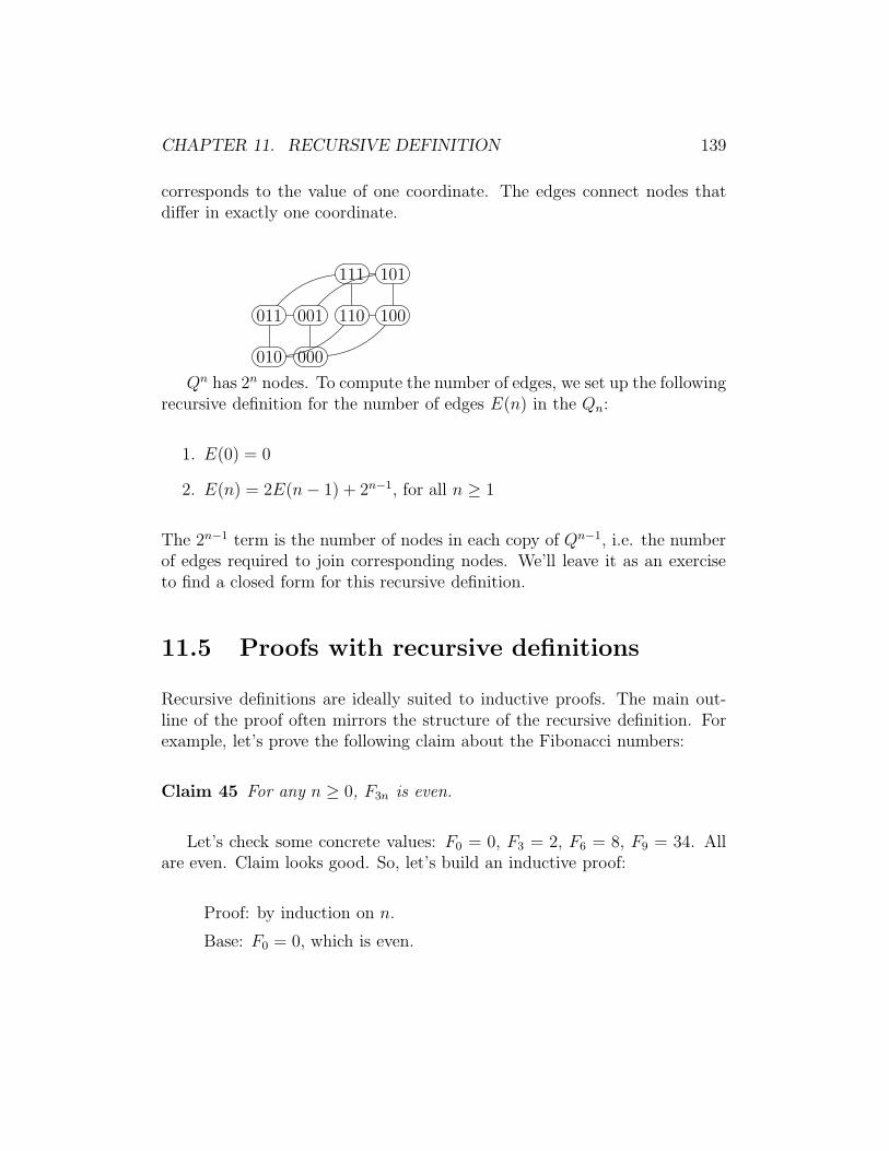
CHAPTER 11. RECURSIVE DEFINITION 139
corresponds to the value of one coordinate. The edges connect nodes thatdiffer in exactly one coordinate.
011
010
001
000
111
110
101
100
Qn has 2n nodes. To compute the number of edges, we set up the followingrecursive definition for the number of edges E(n) in the Qn:
1. E(0) = 0
2. E(n) = 2E(n− 1) + 2n−1, for all n ≥ 1
The 2n−1 term is the number of nodes in each copy of Qn−1, i.e. the numberof edges required to join corresponding nodes. We’ll leave it as an exerciseto find a closed form for this recursive definition.
11.5 Proofs with recursive definitions
Recursive definitions are ideally suited to inductive proofs. The main out-line of the proof often mirrors the structure of the recursive definition. Forexample, let’s prove the following claim about the Fibonacci numbers:
Claim 45 For any n ≥ 0, F3n is even.
Let’s check some concrete values: F0 = 0, F3 = 2, F6 = 8, F9 = 34. Allare even. Claim looks good. So, let’s build an inductive proof:
Proof: by induction on n.
Base: F0 = 0, which is even.

CHAPTER 11. RECURSIVE DEFINITION 140
Induction: Suppose that F3n is even for n = 0, 1, . . . , k. We needto show that F3k is even. We need to show that that F3(k+1) iseven.
F3(k+1) = F3k+3 = F3k+2 + F3k+1
But F3k+2 = F3k+1+F3k. So, substituting into the above equation,we get:
F3(k+1) = (F3k+1 + F3k) + F3k+1 = 2F3k+1 + F3k
By the inductive hypothesis F3k is even. 2F3k+1 is even becauseit’s 2 times an integer. So their sum must be even. So F3(k+1) iseven, which is what we needed to show.
Some people feel a bit uncertain if the base case is a special case like zero.It’s ok to also include a second base case. For this proof, you would check thecase for n = 1 i.e. verify that F3 is even. The extra base case isn’t necessaryfor a complete proof, but it doesn’t cause any harm and may help the reader.
11.6 Inductive definition and strong induc-
tion
Claims involving recursive definitions often require proofs using a string in-ductive hypothesis. For example, suppose that the function f : N → Z isdefined by
f(0) = 2
f(1) = 3
∀n ≥ 1, f(n+ 1) = 3f(n)− 2f(n− 1)
I claim that:
Claim 46 ∀n ∈ N, f(n) = 2n + 1
We can prove this claim as follows:
CHAPTER 11. RECURSIVE DEFINITION 141
Proof: by induction on n.
Base: f(0) is defined to be 2. 20+1 = 1+1 = 2. So f(n) = 2n+1when n = 0.
f(1) is defined to be 3. 21 + 1 = 2 + 1 = 3. So f(n) = 2n + 1when n = 1.
Induction: Suppose that f(n) = 2n + 1 for n = 0, 1, . . . , k.
f(k + 1) = 3f(k)− 2f(k − 1)
By the induction hypothesis, f(k) = 2k+1 and f(k−1) = 2k−1+1.Substituting these formulas into the previous equation, we get:
f(k+1) = 3(2k+1)−2(2k−1+1) = 3 ·2k+3−2k−2 = 2 ·2k+1 =2k+1 + 1
So f(k + 1) = 2k+1 + 1, which is what we needed to show.
We need to use a strong induction hypothesis, as well as two base cases,because the inductive step uses the fact that the formula holds for two pre-vious values of n (k and k − 1).
11.7 Variation in notation
Recursive definitions are sometimes called inductive definitions or (especiallyfor numerical functions) recurrence relations. Folks who call them “recur-rence relations” typically use the term “initial condition” to refer to the basecase.
Chapter 12
Trees
This chapter covers trees and induction on trees.
12.1 Why trees?
Trees are the central structure for storing and organizing data in computerscience. Examples of trees include
• Trees which show the organization of real-world data: family/geneaologytrees, taxonomies (e.g. animal subspecies, species, genera, families)
• Data structures for efficiently storing and retrieving data. The basicidea is the same one we saw for binary search within an array: sort thedata, so that you can repeatedly cut your search area in half.
• Parse trees, which show the structure of a piece of (for example) com-puter program, so that the compiler can correctly produce the corre-sponding machine code.
• Decision trees, which classify data by asking a series of questions. Eachtree node contains a question, whose answer directs you to one of thenode’s children.
For example, here’s a parse tree for the arithmetic expression
142
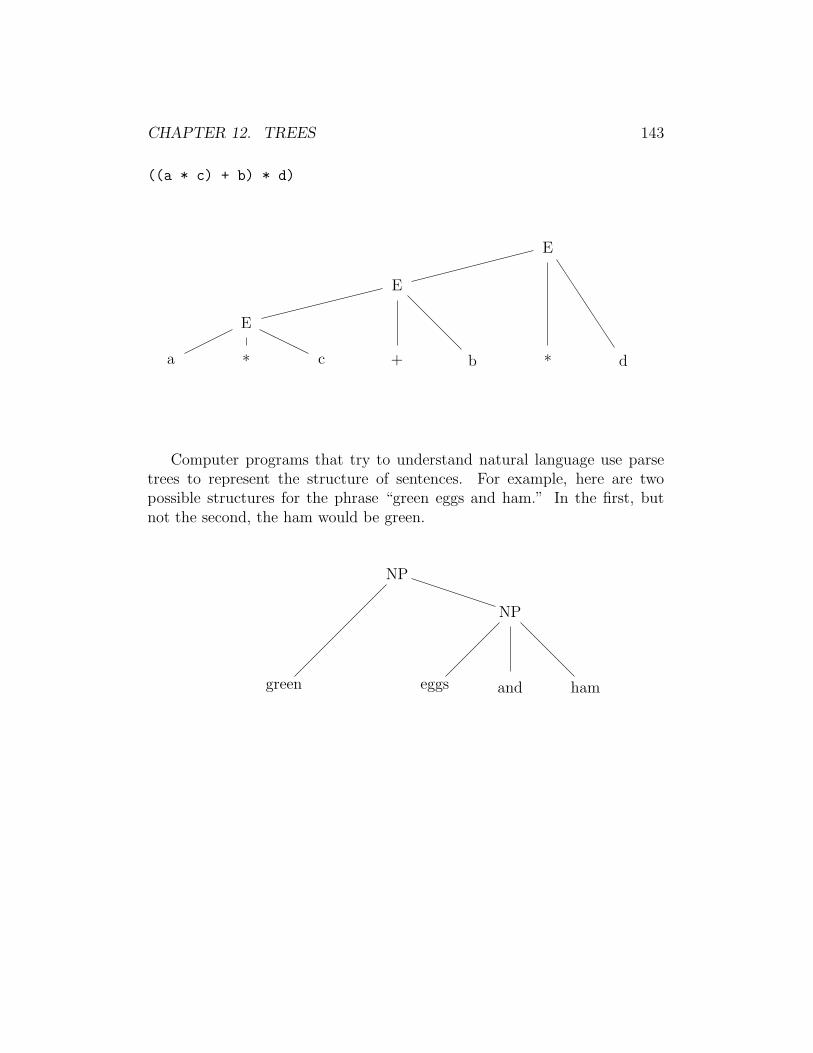
CHAPTER 12. TREES 143
((a * c) + b) * d)
E
E
E
a * c + b * d
Computer programs that try to understand natural language use parsetrees to represent the structure of sentences. For example, here are twopossible structures for the phrase “green eggs and ham.” In the first, butnot the second, the ham would be green.
NP
NP
green eggs and ham
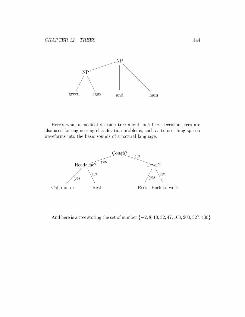
CHAPTER 12. TREES 144
NP
NP
and hamgreen eggs
Here’s what a medical decision tree might look like. Decision trees arealso used for engineering classification problems, such as transcribing speechwaveforms into the basic sounds of a natural language.
Cough?
Headache? Fever?
Call doctor Rest Rest Back to work
yesno
yesno
yesno
And here is a tree storing the set of number {−2, 8, 10, 32, 47, 108, 200, 327, 400}

CHAPTER 12. TREES 145
32
8 108
-2 10 47 327
200 400
12.2 Defining trees
Formally, a tree is a undirected graph with a special node called the root, inwhich every node is connected to the root by exactly one path. When a pairof nodes are neighbors in the graph, the node nearest the root is called theparent and the other node is its child. By convention, trees are drawn withthe root at the top. Two children of the same parent are known as siblings.
To keep things simple, we will assume that the set of nodes in a tree isfinite. We will also assume that each set of siblings is ordered from left toright, because this is common in computer science applications.
A leaf node is a node that has no children. A node that does havechildren is known as an internal node. The root is an internal node, exceptin the special case of a tree that consists of just one node (and no edges).
The nodes of a tree can be organized into levels, based on how manyedges away from the root they are. The root is defined to be level 0. Itschildren are level 1. Their children are level 2, and so forth. The height of atree is the maximum level of any of its nodes or, equivalently, the maximumlevel of any of its leaves or, equivalently, the maximum length of a path fromthe root to a leaf.
CHAPTER 12. TREES 146
If you can get from x to g by following one or more parent links, theng is an ancestor of x and x is a descendent of g. We will treat x as anancestor/descendent of itself. The ancestors/descendents of x other than xitself are its proper ancestors/descendents. If you pick some random nodea in a tree T , the subtree rooted at a consists of a (its root), all of a’sdescendents, and all the edges linking these nodes.
12.3 m-ary trees
Many applications restrict how many children each node can have. A binarytree (very common!) allows each node to have at most two children. An m-ary tree allows each node to have up to m children. Trees with “fat” nodeswith a large bound on the number of children (e.g. 16) occur in some storageapplications.
Important special cases involve trees that are nicely filled out in somesense. In a full m-ary tree, each node has either zero or m children. Neveran intermediate number. So in a full 3-ary tree, nodes can have zero or threechildren, but not one child or two children.
In a complete m-ary tree, all leaves are at the same height. Normally,we’d be interested only in full and complete m-ary trees, where this meansthat the whole bottom level is fully populated with leaves.
For restricted types of trees like this, there are strong relationships be-tween the numbers of different types of notes. for example:
Claim 47 A full m-ary tree with i internal nodes has mi+ 1 nodes total.
To see why this is true, notice that there are two types of nodes: nodeswith a parent and nodes without a parent. A tree has exactly one node withno parent. We can count the nodes with a parent by taking the number ofparents in the tree (i) and multiplying by the branching factor m.
Therefore, the number of leaves in a full m-ary tree with i internal nodesis (mi+ 1)− i = (m− 1)i+ 1.

CHAPTER 12. TREES 147
12.4 Height vs number of nodes
Suppose that we have a binary tree of height h. How many nodes and howmany leaves does it contain? This clearly can’t be an exact formula, sincesome trees are more bushy than others. But we can give useful upper andlower bounds.
To minimize the node counts, consider a tree of height h that has justone leaf. It contains h + 1 nodes connected into a straight line by h edges.So the minimum number of leaves is 1 (regardless of h) and the minimumnumber of nodes is h+ 1.
The node counts are maximized by a tree which is full and complete. Forthese trees, the number of leaves is 2h. More generally, the number of nodesat level L is 2L. So the total number of nodes n is
∑h
L=0 2L. The closed form
for this summation is 2h+1 − 1. So, for full and complete binary trees, theheight is proportional to log2 n.
In a balanced m-ary tree of height h, all leaves are either at height h orat height h − 1. Balanced trees are useful when you want to store n items(where n is some random natural number that might not be a power of 2)while keeping all the leaves at approximately the same height. Balanced treesaren’t as rigid as full binary trees, but they also have height proportional tolog2 n. This means that all the leaves are fairly close to the root, which leadsto good behavior from algorithms trying to store and find things in the tree.
12.5 Context-free grammars
Applications involving languages, both human languages and computer lan-guages, frequently involve parse trees that show the structure of a sequenceof terminals: words or characters. Each node contains a label, which canbe either a terminal or a variable. An internal node or a root node mustbe labelled with a variable; leaves (except for the root) may have either sortof label. To keep things simple, we’ll consistently use uppercase letters forvariables.
For example, the following tree shows one structure for the sequenceof terminals: a*c+b*d. This structure corresponds to adding parentheses

CHAPTER 12. TREES 148
as follows: ((a*c)+b)*d). This tree uses two variables (E and V ) and sixdifferent terminals: a, b, c, d, +, ∗.
E
E
E
V
*
V
+
V
*
V
a c b d
This sort of labelled tree can be conveniently specified by a context-free grammar. A context-free grammar is a set of rules which specify whatsorts of children are possible for a parent node with each type of label. Thelefthand side of each rule gives a label for the parent and the righthand sideshows one possible pattern for the labels on its children. If all the nodes ofa tree T have children matching the rules of some grammar G, we say thatT is generated by G.
For example, the following grammar contains four rules for an E node.The first rule allows an E node to have three children, the leftmost onelabelled E, the middle one labelled + and the right one labelled V . Accordingto these rules, a node labelled V can only have one child, labelled either a,b, c, or d. The tree shown above follows these grammar rules.

CHAPTER 12. TREES 149
E → E + V
E → E ∗ VE → V + V
E → V ∗ VV → a
V → b
V → c
V → d
If a grammar contains several patterns for the children of a certain nodelabel, we can pack them onto one line using a vertical bar to separate theoptions. E.g. we can write this grammar more compactly as
E → E + V | E ∗ V | V + V | V ∗ VV → a | b | c | d
The grammar above allows the root of a tree to be labelled either E orV . Depending on the application, we may wish to restrict the root to haveone specific label, called the start symbol. For example, if we say that E isthe start symbol, then the root must be labelled E but other interior nodesmay be labelled either V or E.
The symbol ǫ is often used for an empty string or sequence. So a rule withǫ on its righthand side specifies that this type of node is allowed to have nochildren. For example, here is a grammar using ǫ and a few trees generatedby it:
S → aSb
S → ǫ
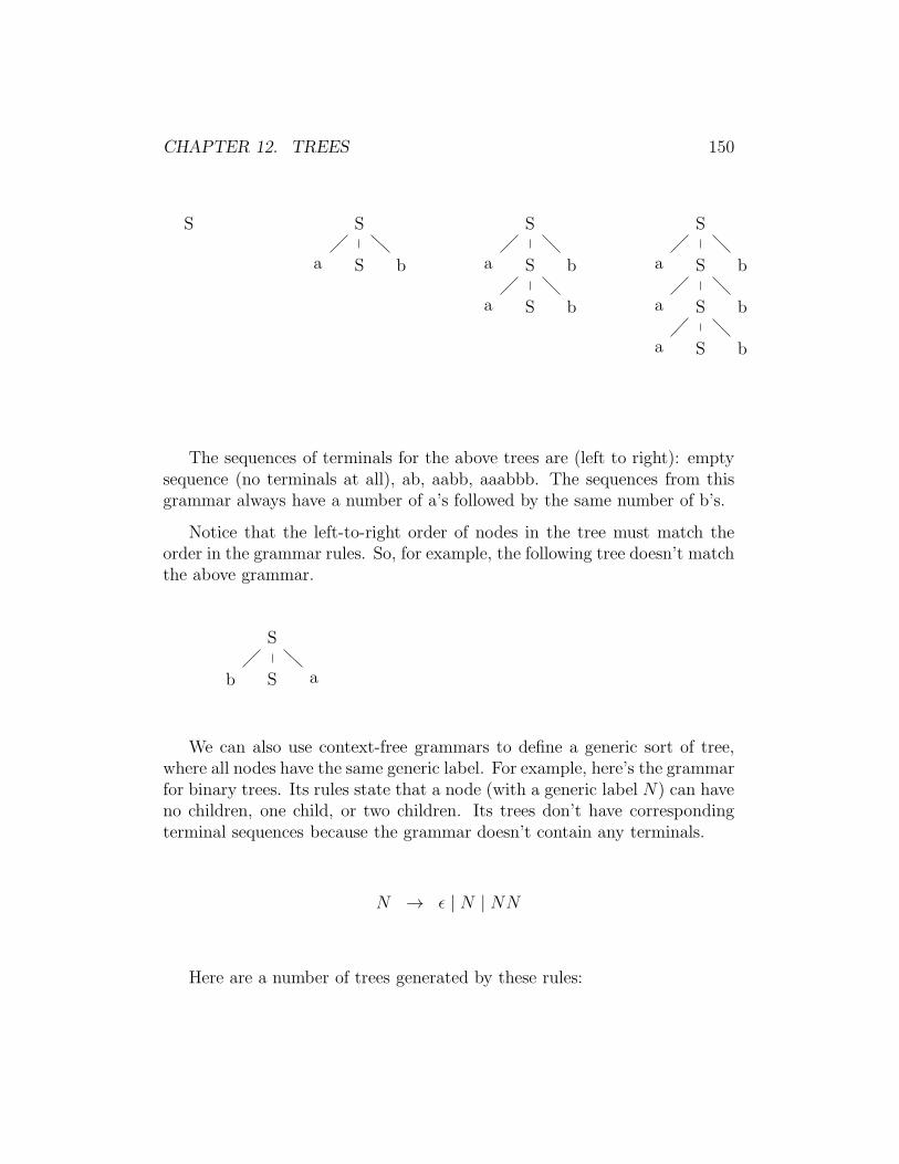
CHAPTER 12. TREES 150
S S
a S b
S
a S b
a S b
S
a S b
a S b
a S b
The sequences of terminals for the above trees are (left to right): emptysequence (no terminals at all), ab, aabb, aaabbb. The sequences from thisgrammar always have a number of a’s followed by the same number of b’s.
Notice that the left-to-right order of nodes in the tree must match theorder in the grammar rules. So, for example, the following tree doesn’t matchthe above grammar.
S
b S a
We can also use context-free grammars to define a generic sort of tree,where all nodes have the same generic label. For example, here’s the grammarfor binary trees. Its rules state that a node (with a generic label N) can haveno children, one child, or two children. Its trees don’t have correspondingterminal sequences because the grammar doesn’t contain any terminals.
N → ǫ | N | NN
Here are a number of trees generated by these rules:
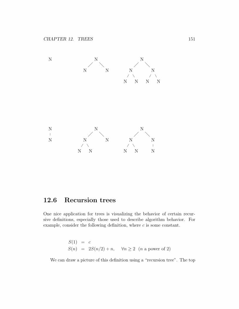
CHAPTER 12. TREES 151
N N
N N
N
N N
N N N N
N
N
N
N N
N N
N
N N
N N N
12.6 Recursion trees
One nice application for trees is visualizing the behavior of certain recur-sive definitions, especially those used to describe algorithm behavior. Forexample, consider the following definition, where c is some constant.
S(1) = c
S(n) = 2S(n/2) + n, ∀n ≥ 2 (n a power of 2)
We can draw a picture of this definition using a “recursion tree”. The top

CHAPTER 12. TREES 152
node in the tree represents S(n) and contains everything in the formula forS(n) except the recursive calls to S. The two nodes below it representtwo copies of the computation of S(n/2). Again, the value in each nodecontains the non-recursive part of the formula for computing S(n/2). Thevalue of S(n) is then the sum of the values in all the nodes in the recursiontree.
n
n/2 n/2
n/4 n/4 n/4 n/4
. . . . . . . . . . . . . . . . . . . . . . . .
To sum everything in the tree, we need to ask:
• How high is this tree, i.e. how many levels do we need to expand beforewe hit the base case n = 1?
• For each level of the tree, what is the sum of the values in all nodes atthat level?
• How many leaf nodes are there?
In this example, the tree has height logn, i.e. there are log n non-leaflevels. At each level of the tree, the node values sum to n. So the sum for allnon-leaf nodes is n log n. There are n leaf nodes, each of which contributes cto the sum. So the sum of everything in the tree is n logn+ cn, which is thesame closed form we found earlier for this recursive definition.
Recursion trees are particularly handy when you only need an approx-imate description of the closed form, e.g. is its leading term quadratic orcubic?
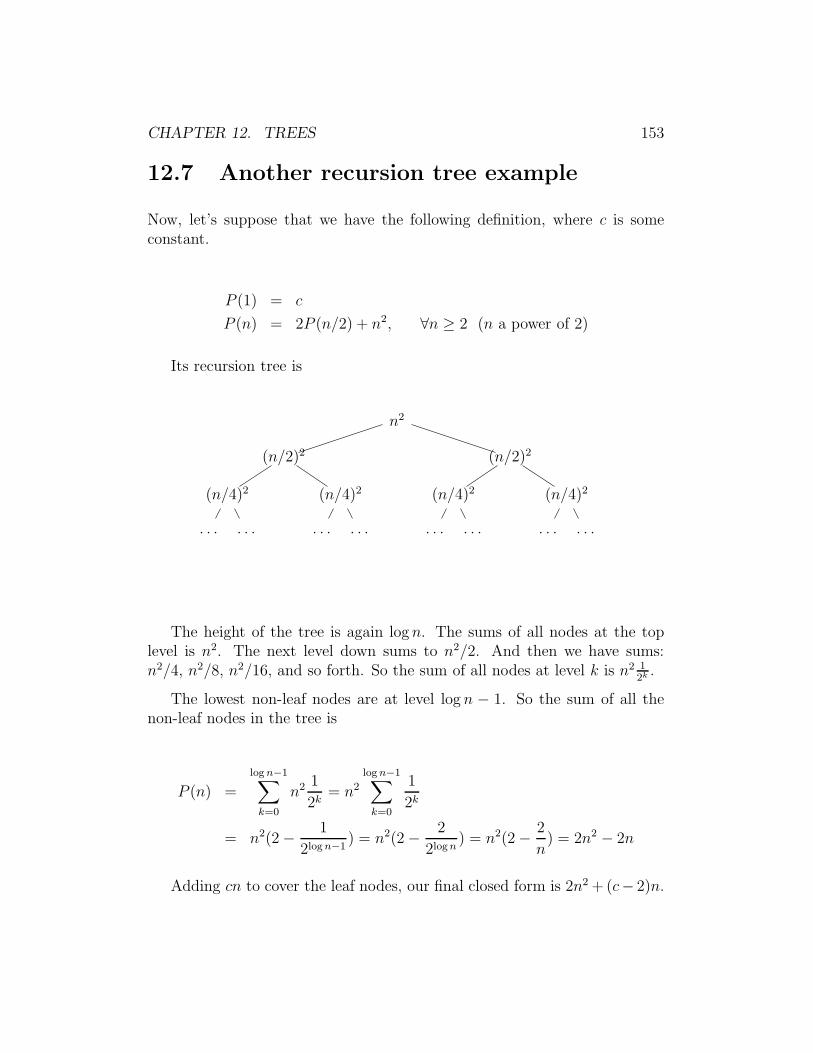
CHAPTER 12. TREES 153
12.7 Another recursion tree example
Now, let’s suppose that we have the following definition, where c is someconstant.
P (1) = c
P (n) = 2P (n/2) + n2, ∀n ≥ 2 (n a power of 2)
Its recursion tree is
n2
(n/2)2 (n/2)2
(n/4)2 (n/4)2 (n/4)2 (n/4)2
. . . . . . . . . . . . . . . . . . . . . . . .
The height of the tree is again logn. The sums of all nodes at the toplevel is n2. The next level down sums to n2/2. And then we have sums:n2/4, n2/8, n2/16, and so forth. So the sum of all nodes at level k is n2 1
2k.
The lowest non-leaf nodes are at level log n − 1. So the sum of all thenon-leaf nodes in the tree is
P (n) =
logn−1∑
k=0
n2 1
2k= n2
logn−1∑
k=0
1
2k
= n2(2− 1
2logn−1) = n2(2− 2
2logn) = n2(2− 2
n) = 2n2 − 2n
Adding cn to cover the leaf nodes, our final closed form is 2n2 +(c− 2)n.

CHAPTER 12. TREES 154
12.8 Tree induction
When doing induction on trees, we divide the tree up at the top. That is, weview a tree as consisting of a root node plus some number of subtrees rootedat its children. The induction variable is typically the height of the tree.The child subtrees have height less than that of the parent tree. So, in theinductive step, we’ll be assuming that the claim is true for these shorter childsubtrees and showing that it’s true for the taller tree that contains them.
For example, we claimed above that
Claim 48 Let T be a binary tree, with height h and n nodes. Then n ≤2h+1 − 1.
Proof by induction on h, where h is the height of the tree.
Base: The base case is a tree consisting of a single node withno edges. It has h = 0 and n = 1. Then we work out that2h+1 − 1 = 21 − 1 = 1 = n.
Induction: Suppose that the claim is true for all binary trees ofheight < h. Let T be a binary tree of height h (h > 0).
Case 1: T consists of a root plus one subtree X . X has heighth− 1. So X contains at most 2h − 1 nodes. T only contains onemore node (its root), so this means T contains at most 2h nodes,which is less than 2h+1 − 1.
r
X
Case 2: T consists of a root plus two subtrees X and Y . X andY have heights p and q, both of which have to be less than h,i.e. ≤ h− 1. X contains at most 2p+1 − 1 nodes and Y containsat most 2q+1 − 1 nodes, by the inductive hypothesis. But, sincep and q are less than h, this means that X and Y each contain≤ 2h − 1 nodes.
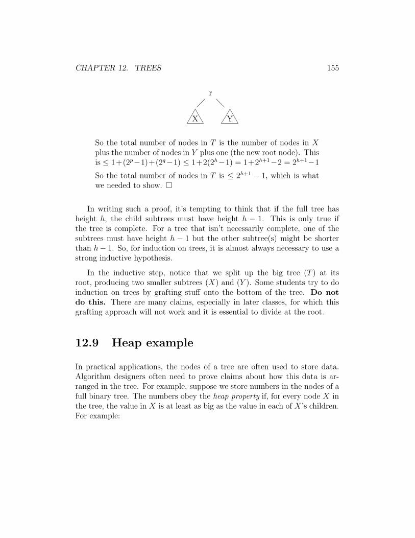
CHAPTER 12. TREES 155
r
X Y
So the total number of nodes in T is the number of nodes in Xplus the number of nodes in Y plus one (the new root node). Thisis ≤ 1+(2p−1)+(2q−1) ≤ 1+2(2h−1) = 1+2h+1−2 = 2h+1−1
So the total number of nodes in T is ≤ 2h+1 − 1, which is whatwe needed to show. �
In writing such a proof, it’s tempting to think that if the full tree hasheight h, the child subtrees must have height h − 1. This is only true ifthe tree is complete. For a tree that isn’t necessarily complete, one of thesubtrees must have height h − 1 but the other subtree(s) might be shorterthan h− 1. So, for induction on trees, it is almost always necessary to use astrong inductive hypothesis.
In the inductive step, notice that we split up the big tree (T ) at itsroot, producing two smaller subtrees (X) and (Y ). Some students try to doinduction on trees by grafting stuff onto the bottom of the tree. Do notdo this. There are many claims, especially in later classes, for which thisgrafting approach will not work and it is essential to divide at the root.
12.9 Heap example
In practical applications, the nodes of a tree are often used to store data.Algorithm designers often need to prove claims about how this data is ar-ranged in the tree. For example, suppose we store numbers in the nodes of afull binary tree. The numbers obey the heap property if, for every node X inthe tree, the value in X is at least as big as the value in each of X ’s children.For example:
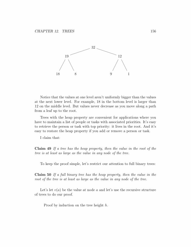
CHAPTER 12. TREES 156
32
19 12
18 8 9 1
Notice that the values at one level aren’t uniformly bigger than the valuesat the next lower level. For example, 18 in the bottom level is larger than12 on the middle level. But values never decrease as you move along a pathfrom a leaf up to the root.
Trees with the heap property are convenient for applications where youhave to maintain a list of people or tasks with associated priorities. It’s easyto retrieve the person or task with top priority: it lives in the root. And it’seasy to restore the heap property if you add or remove a person or task.
I claim that:
Claim 49 If a tree has the heap property, then the value in the root of thetree is at least as large as the value in any node of the tree.
To keep the proof simple, let’s restrict our attention to full binary trees:
Claim 50 If a full binary tree has the heap property, then the value in theroot of the tree is at least as large as the value in any node of the tree.
Let’s let v(a) be the value at node a and let’s use the recursive structureof trees to do our proof.
Proof by induction on the tree height h.
CHAPTER 12. TREES 157
Base: h = 0. A tree of height zero contains only one node, soobviously the largest value in the tree lives in the root!
Induction: Suppose that the claim is true for all full binary treesof height < h. Let T be a tree of height h (h > 0) which has theheap property. Since T is a full binary tree, its root r has twochildren p and q. Suppose that X is the subtree rooted at p andY is the subtree rooted at q.
Both X and Y have height < h. Moreover, notice that X and Ymust have the heap property, because they are subtrees of T andthe heap property is a purely local constraint on node values.
Suppose that x is any node of T . We need to show that v(r) ≥v(x). There are three cases:
Case 1: x = r. This is obvious.
Case 2: x is any node in the subtree X . Since X has the heapproperty and height≤ h, v(p) ≥ v(x) by the inductive hypothesis.But we know that v(r) ≥ v(p) because T has the heap property.So v(r) ≥ v(x).
Case 3: x is any node in the subtree Y . Similar to case 2.
So, for any node x in T , v(r) ≥ v(x).�
12.10 Proof using grammar trees
Consider the following grammar G. I claim that all trees generated by Ghave the same number of nodes with label a as with label b.
S → ab
S → SS
S → aSb
We can prove this by induction as follows:
CHAPTER 12. TREES 158
Proof by induction on the tree height h.
Base: Notice that trees from this grammar always have height atleast 1. The only way to produce a tree of height 1 is from thefirst rule, which generates exactly one a node and one b node.
Induction: Suppose that the claim is true for all trees of height< k, where k ≥ 1. Consider a tree T of height k. The root mustbe labelled S and the grammar rules give us three possibilitiesfor what the root’s children look like:
Case 1: The root’s children are labelled a and b. This is just thebase case.
Case 2: The root’s children are both labelled S. The subtreesrooted at these children have height < k. So, by the inductivehypothesis, each subtree has equal numbers of a and b nodes. Saythat the left tree has m of each type and the right tree has n ofeach type. Then the whole tree has m+ n nodes of each type.
Case 3: The root has three children, labelled a, S, and b. Sincethe subtree rooted at the middle child has height < k, it has equalnumbers of a and b nodes by the inductive hypothesis. Supposeit has m nodes of each type. Then the whole tree has m+1 nodesof each type.
In all three cases, the whole tree T has equal numbers of a and bnodes.
12.11 Variation in terminology
There are actually two sorts of trees in the mathematical world. This chapterdescribes the kind of trees most commonly used in computer science, whichare formally “rooted trees” with a left-to-right order. In graph theory, theterm “tree” typically refers to “free trees,” which are connected acyclic graphswith no distinguished root node and no clear up/down or left-right directions.We will see free trees later, when analyzing planar graphs. Variations on thesetwo types of trees also occur. For example, some data structures applicationsuse trees that are almost like ours, except that a single child node must bedesignated as a “left” or “right” child.

CHAPTER 12. TREES 159
Infinite trees occur occasionally in computer science applications. Theyare an obvious generalization of the finite trees discussed here.
Tree terminology varies a lot, apparently because trees are used for a widerange of applications with very diverse needs. In particular, some authors usethe term “complete binary tree” to refer to a tree in which only the leftmostpart of the bottom level is filled in. The term “perfect” is then used for atree whose bottom level is entirely filled. Some authors don’t allow a nodeto be an ancestor or descendent of itself. A few authors don’t consider theroot node to be a leaf.
Chapter 13
Big-O
This chapter covers asymptotic analysis of function growth and big-O nota-tion.
13.1 Running times of programs
An important aspect of designing a computer programs is figuring out howwell it runs, in a range of likely situations. Designers need to estimate howfast it will run, how much memory it will require, how reliable it will be, andso forth. In this class, we’ll concentrate on speed issues.
Designers for certain small platforms sometimes develop very detailedmodels of running time, because this is critical for making complex appli-cations work with limited resources. E.g. making God of War run on yourIphone. However, such programming design is increasingly rare, becausecomputers are getting fast enough to run most programs without hand opti-mization.
More typically, the designer has to analyze the behavior of a large C orJava program. It’s not feasible to figure out exactly how long such a pro-gram will take. The transformation from standard programming languagesto machine code is way too complicated. Only rare programmers have aclear grasp of what happens within the C or Java compiler. Moreover, a verydetailed analysis for one computer system won’t translate to another pro-
160
CHAPTER 13. BIG-O 161
gramming language, another hardware platform, or a computer purchaseda couple years in the future. It’s more useful to develop an analysis thatabstracts away from unimportant details, so that it will be portable anddurable.
This abstraction process has two key components:
• Ignore multiplicative constants
• Ignore behavior on small inputs, concentrating on how well programshandle large inputs. (Aka asymptotic analysis.)
Multiplicative constants are extremely sensitive to details of the imple-mentation, hardware platform, etc.
Behavior on small inputs is ignored, because programs typically run fastenough on small test cases. Or will do so soon, as computers become fasterand faster. Hard-to-address problems more often arise when a program’suse expands to larger examples. For example, a small database programdeveloped for a community college might have trouble coping if deployed tohandle (say) all registration records for U. Illinois.
13.2 Function growth: the ideas
So, suppose that you model the running time of a program as a functionF (n), where n is some measure of the size of the input problem. E.g. nmight be the number of entries in a database application. For a numericalprogram, n might be the magnitude or the number of digits in an inputnumber. Then, to compare the running times of two programs, we need tocompare the growth rates of the two running time functions.
So, suppose we have two functions f and g, whose inputs and outputsare real numbers. Which one has “bigger outputs”?
Suppose that f(x) = x and g(x) = x2. For small positive inputs, x2 issmaller. For the input 1, they have the same value, and then g gets biggerand rapidly diverges to become much larger than f . We’d like to say that gis “bigger,” because it has bigger outputs for large inputs.
CHAPTER 13. BIG-O 162
Because we are only interested in the running times of algorithms, we’llonly consider behavior on positive inputs. And we’ll only worry about func-tions whose output values are positive, or whose output values become pos-itive as the input value gets big, e.g. the log function.
Because we don’t care about constant multipliers, we’ll consider functionssuch as 3x2, 47x2, and 0.03x2 to all grow at the same rate. Similarly, functionssuch as 3x, 47x, and 0.03x will be treated as growing at the same, slower,rate. The functions in each group don’t all have the same slope, but theirgraphs have the same shape as they head off towards infinity. That’s theright level of approximation for analyzing most computer programs.
Finally, when a function is the sum of faster and slower-growing terms,we’ll only be interested in the faster-growing term. For example, 0.3x2 +7x + 105 will be treated as equivalent to x2. As the input x gets large, thebehavior of the function is dominated by the term with the fastest growth(the first term in this case).
13.3 Primitive functions
Let’s look at some basic functions and try to put them into growth order.
Any constant function grows more slowly than a linear function (i.e. be-cause a constant function doesn’t grow!). A linear polynomial grows moreslowly than a quadratic. For large numbers, a third-order polynomial growsfaster than a quadratic.
Earlier in the term (as an example of an induction proof), we showed that2n ≤ n! for every integer n ≥ 4. Informally, this is true because 2n and n!are each the product of n terms. For 2n, they are all 2. For n! they are thefirst n integers, and all but the first two of these are bigger than 2. Althoughwe only proved this inequality for integer inputs, you’re probably preparedto believe that it also holds for all real inputs ≥ 4.
In a similar way, you can use induction to show that n2 < 2n for anyinteger n ≥ 4. And, in general, for any exponent k, you can show that nk < 2n
for any n above some suitable lower bound. And, again, the intermediatereal input values follow the same pattern. You’re probably familiar with how
CHAPTER 13. BIG-O 163
fast exponentials grow. There’s a famous story about a judge imposing adoubling-fine on a borough of New York, for ignoring the judge’s orders. Ittook the borough officials a few days to realize that this was serious badnews, at which point a settlement was reached.
So, 2n grows faster than any polynomial in n, and n! grows yet faster. Ifwe use 1 as our sample constant function, we can summarize these facts as:
1 ≺ n ≺ n2 ≺ n3 . . . ≺ 2n ≺ n!
I’ve used curly ≺ because this ordering isn’t standard algebraic ≤. Theordering only works when n is large enough.
For the purpose of designing computer programs, only the first three ofthese running times are actually good news. Third-order polynomials alreadygrow too fast for most applications, if you expect inputs of non-trivial size.Exponential algorithms are only worth running on extremely tiny inputs, andare frequently replaced by faster algorithms (e.g. using statistical sampling)that return approximate results.
Now, let’s look at slow-growing functions, i.e. functions that might bethe running times of efficient programs. We’ll see that algorithms for findingentries in large datasets often have running times proportional to logn. Ifyou draw the log function and ignore its strange values for inputs smallerthan 1, you’ll see that it grows, but much more slowly than n.
Algorithms for sorting a list of numbers have running times that growlike n log n. If n is large enough, 1 < logn < n. So n < n logn < n2. We cansummarize these relationships as:
1 ≺ log n ≺ n ≺ n logn ≺ n2
It’s well worth memorizing the relative orderings of these basic functions,since you’ll see them again and again in this and future CS classes.
CHAPTER 13. BIG-O 164
13.4 The formal definition
Let’s write out the formal definition. Suppose that f and g are functionswhose domain and co-domain are subsets of the real numbers. Then f(x) isO(g(x)) (read “big-O of g) if and only if
There are positive real numbers c and k such that 0 ≤ f(x) ≤cg(x) for every x ≥ k.
The constant c in the equation models the fact that we don’t care aboutmultiplicative constants in comparing functions. The restriction that theequation only holds for x ≥ k models the fact that we don’t care about thebehavior of the functions on small input values.
So, for example, 3x2 is O(2x). 3x2 is also O(x2). But 3x2 is not O(x). Sothe big-O relationship includes the possibility that the functions grow at thesame rate.
When g(x) is O(f(x)) and f(x) is O(g(x)), then f(x) and g(x) must growat the same rate. In this case, we say that f(x) is Θ(g(x)) (and also g(x) isΘ(f(x))).
Big-O is a partial order on the set of all functions from the reals tothe reals. The Θ relationship is an equivalence relation on this same set offunctions. So, for example, under the Θ relation, the equivalence class [x2]contains functions such as x2, 57x2 − 301, 2x2 + x+ 2, and so forth.
13.5 Applying the definition
To show that a big-O relationship holds, we need to produce suitable valuesfor c and k. For any particular big-O relationship, there are a wide rangeof possible choices. First, how you pick the multiplier c affects where thefunctions will cross each other and, therefore, what your lower bound k canbe. Second, there is no need to minimize c and k. Since you are just demon-strating existence of suitable c and k, it’s entirely appropriate to use overkillvalues.
CHAPTER 13. BIG-O 165
For example, to show that 3x is O(x2), we can pick c = 3 and k = 1.Then 3x ≤ cx2 for every x ≥ k translates into 3x ≤ 3x2 for every x ≥ 1,which is clearly true. But we could have also picked c = 100 and k = 100.
Overkill seems less elegant, but it’s easier to confirm that your chosenvalues work properly, especially in situations like exams. Moreover, slightlyoverlarge values are often more convincing to the reader, because the readercan more easily see that they do work.
To take a more complex example, let’s show that 3x2 + 7x + 2 is O(x2).If we pick c = 3, then our equation would look like 3x2 +7x+2 ≤ 3x2. Thisclearly won’t work for large x.
So let’s try c = 4. Then we need to find a lower bound on x that makes3x2 + 7x+ 2 ≤ 4x2 true. To do this, we need to force 7x+ 2 ≤ x2. This willbe true if x is big, e.g. ≥ 100. So we can choose k = 100.
To satisfy our formal definition, we also need to make sure that bothfunctions produce positive values for all inputs ≥ k. If this isn’t already thecase, increase k.
13.6 Writing a big-O proof
In a formal big-O proof, you first choose values for k and c, then show that0 ≤ f(x) ≤≤ cg(x) for every x ≥ k. So the example from the previoussection would look like:
Claim 51 3x2 + 7x+ 2 is O(x2).
Proof: Consider c = 4 and k = 100. Then for any x ≥ k, x2 ≥100x ≥ 7x+2. Since x is positive, we also have 0 ≤ 3x2+7x+2.Therefore, for any x ≥ k, 0 ≤ 3x2+7x+2 ≤ 3x2+x2 = 4x2 = cx2.So 3x2 + 7x+ 2 is O(x2).
Notice that the steps of this proof are in the opposite order from the workwe used to find values for c and k. This is standard for big-O proofs. Counton writing them in two drafts (e.g. the first on scratch paper).
Here’s another example of a big-O proof:
CHAPTER 13. BIG-O 166
Claim 52 Show that 3x2 + 8x log x is O(x2).
[On our scratch paper] x log x ≤ x2 for any x ≥ 1. So 3x2 + 8x log x ≤11x2. So if we set c = 11 and k = 1, our definition of big-O is satisfied.
Writing this out neatly, we get:
Proof: Consider c = 11 and k = 1. Suppose that x ≥ k. Thenx ≥ 1. So 0 ≤ log x ≤ x. Since x is positive, this implies that0 ≤ x log x ≤ x2. So then 0 ≤ 3x2 + 8x log x ≤ 11x2 = cx, whichis what we needed to show.
13.7 Sample disproof
Suppose that we want to show that a big-O relationship does not hold. We’retrying to prove that suitable values of c and k cannot exist. Like many non-existence claims, this is best attacked using proof by contradiction.
For example:
Claim 53 x3 is not O(7x2).
Proof by contradiction. Suppose x3 were O(7x2). Then there arec and k such that 0 ≤ x3 ≤ c7x2 for every x ≥ k. But x3 ≤ c7x2
implies that x ≤ 7c. But this fails for values of x that are greaterthan 7c. So we have a contradiction.
13.8 Variation in notation
In the definition of big-o, some authors replace 0 ≤ f(x) ≤ cg(x) with|f(x)| ≤ c|g(x)|. The absolute values and the possibility of negative valuesmakes this version harder to work with. Some authors state the definitiononly for functions f and g with positive output values. This is awkwardbecause the logarithm function produces negative output values for very smallinputs.

CHAPTER 13. BIG-O 167
Outside theory classes, computer scientists often say that f(x) is O(g(x))when they actually mean the (stronger) statement that f(x) is Θ(g(x)). Or—this drives theoreticians nuts—they will say that g(x) is a “tight” big-Obound on f(x). In this class, we’ll stick to the proper theory notation, sothat you can learn how to use it. That is, use Θ when you mean to say thattwo functions grow at the same rate or when you mean to give a tight bound.
Very, very annoyingly, for historical reasons, the statement f(x) isO(g(x))is often written as f(x) = O(g(x)). This looks like a sort of equality, but itisn’t. It is actually expressing an inequality. This is badly-designed notationbut, sadly, common.

Chapter 14
Algorithms
This chapter covers how to analyze the running time of algorithms.
14.1 Introduction
The techniques we’ve developed earlier in this course can be applied to ana-lyze how much time a computer algorithm requires, as a function of the sizeof its input(s). We will see a range of simple algorithms illustrating a varietyof running times. Three methods will be used to analyze the running times:nested loops, resource consumption, and recursive definitions.
We will figure out only the big-O running time for each algorithm, i.e.ignoring multiplicative constants and behavior on small inputs. This willallow us to examine the overall design of the algorithms without excessivecomplexity. Being able to cut corners so as to get a quick overview is acritical skill when you encounter more complex algorithms in later computerscience classes.
14.2 Basic data structures
Many simple algorithms need to store a sequence of objects a1, . . . , an. Inpseudocode, the starting index for a sequence is sometimes 0 and sometimes
168

CHAPTER 14. ALGORITHMS 169
1, and you often need to examine the last subscript to find out the length.Sequences can be stored using either an array or a linked list. The choicesometimes affects the algorithm analysis, because these two implementationmethods have slightly different features.
An array provides constant-time access to any element. So you canquickly access elements in any order you choose and the access time doesnot depend on the length of the list. However, the length of an array is fixedwhen the array is built. Changing the array length takes time proportionalto the length of the array, i.e. O(n). Adding or deleting objects in the middleof the array requires pushing other objects sideways. This can also take O(n)time. Two-dimensional arrays are similar, except that you need to supplytwo subscripts e.g. ax,y.
In a linked list, each object points to the next object in the list. Analgorithm has direct access only to the elements at the ends of the list.1
Objects in the middle of the list can only be accessed by walking element-by-element from one end, which can take O(n) time. However, the lengthof the list is flexible and objects can added to, or removed from, the ends ofthe list in constant time. Once you are at a position in the middle of a list,objects can be added or deleted at that position in constant time.
A linked list starts with its head and ends with its tail. For example,suppose our list is L = (1, 7, 3, 4, 7, 19). Then head(L) is 1 and tail(L) is 19.The function pop removes and returns the value at the head of a list. I.e.pop(L) will return 1 leave the list L containing (7, 3, 4, 7, 19).
For some algorithms, the big-O performance does not depend on whetherarrays or linked lists are used. This happens when the number of objects isfixed and the objects are accessed in sequential order. However, rememberthat a big-O analysis ignores multiplicative constants. All other things be-ing equal, array-based implementations tend to have smaller constants andtherefore run faster.
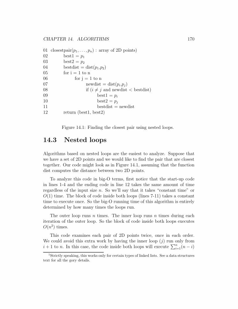
CHAPTER 14. ALGORITHMS 170
01 closestpair(p1, . . . , pn) : array of 2D points)02 best1 = p103 best2 = p204 bestdist = dist(p1,p2)05 for i = 1 to n06 for j = 1 to n07 newdist = dist(pi,pj)08 if (i 6= j and newdist < bestdist)09 best1 = pi10 best2 = pj11 bestdist = newdist12 return (best1, best2)
Figure 14.1: Finding the closest pair using nested loops.
14.3 Nested loops
Algorithms based on nested loops are the easiest to analyze. Suppose thatwe have a set of 2D points and we would like to find the pair that are closesttogether. Our code might look as in Figure 14.1, assuming that the functiondist computes the distance between two 2D points.
To analyze this code in big-O terms, first notice that the start-up codein lines 1-4 and the ending code in line 12 takes the same amount of timeregardless of the input size n. So we’ll say that it takes “constant time” orO(1) time. The block of code inside both loops (lines 7-11) takes a constanttime to execute once. So the big-O running time of this algorithm is entirelydetermined by how many times the loops run.
The outer loop runs n times. The inner loop runs n times during eachiteration of the outer loop. So the block of code inside both loops executesO(n2) times.
This code examines each pair of 2D points twice, once in each order.We could avoid this extra work by having the inner loop (j) run only fromi+ 1 to n. In this case, the code inside both loops will execute
∑n
i=1(n− i)
1Strictly speaking, this works only for certain types of linked lists. See a data structures
text for all the gory details.

CHAPTER 14. ALGORITHMS 171
times. This is equal to∑n−1
i=0 i = n(n−1)2
. This is still O(n2): our optimizationimproved the constants but not the big-O running time. Improving the big-O running time—O(n logn) is possible–requires restructuring the algorithmand involves some geometrical detail beyond the scope of this chapter.
14.4 Merging two lists
01 merge(L1,L2: sorted lists of real numbers)02 O = emptylist03 while (L1 is not empty or L2 is not empty)04 if (L1 is empty)05 move head(L2) to the tail of O06 else if (L2 is empty)07 move head(L1) to the tail of O08 else if (head(L1) <= head(L2))09 move head(L1) to the tail of O10 else move head(L2) to the tail of O11 return O
Figure 14.2: Merging two lists
When code contains a while loop, rather than a for loop, it can be lessobvious how many times the loop will run. For example, suppose we have twosorted lists, a1, . . . , ap and b1, . . . , bq. We can merge them very efficientlyinto a combined sorted list. To do this, we make a new third empty listto contain our merged output. Then we examine the first elements of thetwo input lists and move the smaller value onto our output list. We keeplooking at the first elements of both lists until one list is empty. We thencopy over the rest of the non-empty list. Figure 14.2 shows pseudocode forthis algorithm.
For merge, a good measure of the size of the input is the length of theoutput array n, which is equal to the sum of the lengths of the two inputarrays (p + q). The merge function has one big while loop. Since the op-erations within the loop (lines 4-10) all take constant time, we just need tofigure out how many times the loop runs, as a function of n.

CHAPTER 14. ALGORITHMS 172
A good way to analyze while loops is to track a resource that has a knownsize and is consumed as the loop runs. In this case, each time the loop runs,we move one number from L1 or L2 onto the output list O. We have nnumbers to move, after while the loop halts. So the loop must run n times.So merge takes O(n) (aka linear) time. This is called a resource consumptionanalysis.
14.5 A reachability algorithm
The function in Figure 14.3 determines whether one node t in a graph isreachable from another node s, i.e. whether there is a path connecting s andt. To do this, we start from s and explore outwards by following the edgesof the graph. When we visit a node, we place a marker on it so that wecan avoid examining it again (and thereby getting the code into an infiniteloop). The temporary list M contains nodes that we have reached, but whoseneighbors have not yet been explored.2
01 reachable(G: a graph; s,t: nodes in G)02 if s = t return true03 Unmark all nodes of G.04 M = emptylist05 Mark node s and add it to M06 while (M is not empty)07 p = pop(M)08 for every node q that is a neighbor of p in G09 if q = t return true10 else if q is not marked, mark q and add it to M11 return false
Figure 14.3: Can node s be reached from node t?
We can use a resource consumption argument to analyze the while loopin this code. Suppose that G has n nodes and m edges. No node is put onto
2Line 5 is deliberately vague about which end of M the nodes are added to and,
therefore, vague about the order in which nodes are explored.
CHAPTER 14. ALGORITHMS 173
the list M more than once. So the loop in lines 6-10 runs no more than ntimes.
Line 8 starts at a node q and find all its neighbors p. So it traces all theedges involving q. During the whole run of the code, a graph edge might gettraced twice, once in each direction. There are m edges in the graph. Solines 9-10 cannot run more than 2m times.
In total, this algorithm needs O(n+m) time. This is an interesting casebecause neither of the two terms n or m dominates the other. It is truethat the number of edges m is no O(n2) and thus the connected componentalgorithm is O(n2). However, in most applications, relatively few of thesepotential edges are actually present. So the O(n+m) bound is more helpful.
Notice that there is a wide variety of graphs with n nodes and m edges.Our analysis was based on the kind of graph that wold causes the algorithmto run for the longest time, i.e. a graph in which the algorithm reaches everynode and traverses every edge, reaching t last. This is called a worst-caseanalysis. On some input graphs, our code might run much more quickly, e.g.if we encounter t early in the search or if much of the graph is not connected tos. Unless the author explicitly indicates otherwise, big-O algorithm analysesare normally understood to be worst-case.
14.6 Binary search
We will now look at a strategy for algorithm design called “divide and con-quer,” in which a larger problem is solved by dividing it into several (usuallytwo) smaller problems. For example, the code in Figure 14.4 uses a techniquecalled binary search to calculate the square root of its input. For simplicity,we’ll assume that the input n is quite large, so that we only need the answerto the nearest integer.
This code operates by defining a range of integers in which the answermust live, initially between 1 and n. Each recursive call tests whether themidpoint of the range is higher or lower than the desired answer, and selectsthe appropriate half of the range for further exploration. The helper functionsquarerootrec returns when it has found ⌊
√
(n)⌋. The function then checkswhether this value, or the next higher integer, is the better approximation.
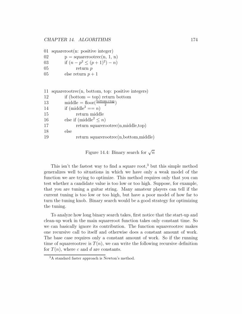
CHAPTER 14. ALGORITHMS 174
01 squareroot(n: positive integer)02 p = squarerootrec(n, 1, n)03 if (n− p2 ≤ (p+ 1)2)− n)05 return p05 else return p+ 1
11 squarerootrec(n, bottom, top: positive integers)12 if (bottom = top) return bottom13 middle = floor(bottom+top
2)
14 if (middle2 == n)15 return middle16 else if (middle2 ≤ n)17 return squarerootrec(n,middle,top)18 else19 return squarerootrec(n,bottom,middle)
Figure 14.4: Binary search for√n
This isn’t the fastest way to find a square root,3 but this simple methodgeneralizes well to situations in which we have only a weak model of thefunction we are trying to optimize. This method requires only that you cantest whether a candidate value is too low or too high. Suppose, for example,that you are tuning a guitar string. Many amateur players can tell if thecurrent tuning is too low or too high, but have a poor model of how far toturn the tuning knob. Binary search would be a good strategy for optimizingthe tuning.
To analyze how long binary search takes, first notice that the start-up andclean-up work in the main squareroot function takes only constant time. Sowe can basically ignore its contribution. The function squarerootrec makesone recursive call to itself and otherwise does a constant amount of work.The base case requires only a constant amount of work. So if the runningtime of squarerootrec is T (n), we can write the following recursive definitionfor T (n), where c and d are constants.
3A standard faster approach is Newton’s method.

CHAPTER 14. ALGORITHMS 175
• T (1) = c
• T (n) = T (n/2) + d
If we unroll this definition k times, we get T (n) = T ( n2k) + kd. Assuming
that n is a power of 2, we hit the base case when k = log n. So T (n) =c+ d logn, which is O(logn).
14.7 Mergesort
Mergesort takes an input linked list of numbers and returns a new linked listcontaining the sorted numbers. This is somewhat different from bubble andinsertion sort, which rearrange the values within a single array (and don’treturn anything).
Mergesort divides its big input list (length n) into two smaller lists oflength n/2. Lists are divided up repeatedly until we have a large number ofvery short lists, of length 1 or 2 (depending on the preferences of the codewriter). A length-1 list is necessarily sorted. A length 2 list can be sortedin constant time. Then, we take all these small sorted lists and merge themtogether in pairs, gradually building up longer and longer sorted lists until wehave one sorted list containing all of our original input numbers. Figure 14.5shows the resulting pseudocode.
01 mergesort(L = a1, a2, . . . , an: list of real numbers)02 if (n = 1) then return L03 else04 m = ⌊n/2⌋05 L1 = (a1, a2, . . . , am)06 L2 = (am+1, am+2, . . . , an)07 return merge(mergesort(L1),mergesort(L2))
Figure 14.5: Sorting a list using mergesort
On an input of length n, mergesort makes two recursive calls to itself. Italso does O(n) work dividing the list in half, because it must walk, elementby element, from the head of the list down to the middle position. And it
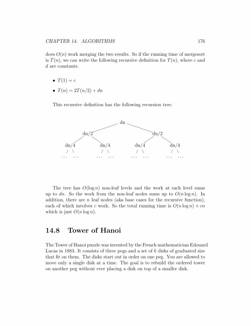
CHAPTER 14. ALGORITHMS 176
does O(n) work merging the two results. So if the running time of mergesortis T (n), we can write the following recursive definition for T (n), where c andd are constants.
• T (1) = c
• T (n) = 2T (n/2) + dn
This recursive definition has the following recursion tree:
dn
dn/2 dn/2
dn/4 dn/4 dn/4 dn/4
. . . . . . . . . . . . . . . . . . . . . . . .
The tree has O(logn) non-leaf levels and the work at each level sumsup to dn. So the work from the non-leaf nodes sums up to O(n logn). Inaddition, there are n leaf nodes (aka base cases for the recursive function),each of which involves c work. So the total running time is O(n logn) + cnwhich is just O(n logn).
14.8 Tower of Hanoi
The Tower of Hanoi puzzle was invented by the French mathematician EdouardLucas in 1883. It consists of three pegs and a set of k disks of graduated sizethat fit on them. The disks start out in order on one peg. You are allowed tomove only a single disk at a time. The goal is to rebuild the ordered toweron another peg without ever placing a disk on top of a smaller disk.

CHAPTER 14. ALGORITHMS 177
The best way to understand the solution is recursively. Suppose thatwe know how to move k disks from one peg to another peg, using a thirdtemporary-storage peg. To move k + 1 disks from peg A to peg B using athird peg C, we first move the top k disks from A to C using B as temporarystorage. Then we move the biggest disk from A to B. Then we move theother k disks from C to B, using A as temporary storage. So our recursivesolver would have pseudocode as in Figure 14.6.
01 hanoi(A,B,C: pegs, d1, d2 . . . dn: disks)02 if (n = 1) move d1 = dn from A to B.03 else04 hanoi(A,C,B,d1, d2, . . . dn−1)05 move dn from A to B.06 hanoi(C,B,A,d1, d2, . . . dn−1)
Figure 14.6: Solving the Towers of Hanoi problem
The function hanoi breaks up a problem of size n into two problems ofsize n−1. Alert! Warning bells! This can’t be good: the sub-problems aren’tmuch smaller than the original problem!
Anyway, hanoi breaks up a problem of size n into two problems of sizen− 1. Other than the two recursive calls, it does only a constant amount ofwork. So the running time T (n) for the function hanoi would be given bythe recursive definition (where c and d are constants):
• T (1) = c
• T (n) = 2T (n− 1) + d
If we unroll this definition, we get
CHAPTER 14. ALGORITHMS 178
T (n) = 2T (n− 1) + d
= 2 · 2(T (n− 2) + d) + d
= 2 · 2(2(T (n− 3) + d) + d) + d
= 23T (n− 3) + 22d+ 2d+ d
= 2kT (n− k) + d
k−1∑
i=0
2i
We’ll hit the base case when k = n− 1. So
T (n) = 2kT (n− k) + d
k−1∑
i=0
2i
= 2n−1c + d
n−2∑
i=0
2i
= 2n−1c + d(2n−1 − 1)
= 2n−1c + 2n−1d− d
= O(2n)
14.9 Multiplying big integers
Suppose we want to multiply two integers. Back in the Bad Old Days of slowcomputers, we would need to multiply moderate-sized integers digit-by-digit.These days, we typically have a CPU that can multiply two moderate-sizednumbers (e.g. 16-bit, 32-bit) as a single operation. But some applications(e.g. in cryptography) involve multiplying very, very large integers. Eachvery long integer must then be broken up into a sequence of 16-bit or 32-bitintegers.
Let’s suppose that we are breaking up each integer into individual digits,and that we’re working in base 2. The recursive multiplication algorithmdivides each n-digit input number into two n/2-digit halves. Specifically,
CHAPTER 14. ALGORITHMS 179
suppose that our input numbers are x and y and they each have 2m digits.We can then divide them up as
x = x12m + x0
y = y12m + y0
If we multiply x by y in the obvious way, we get
xy = A22m +B2m + C
where A = x1y1, B = x0y1+x1y0, and C = x0y0. Set up this way, computingxy requires multiplying four numbers with half the number of digits.
So, if you just count the number of multiplications, the running time ofthis naive method has the recursive definition:
• T (1) = c
• T (n) = 4T (n/2) +O(n)
The closed form for T (n) is O(n2) (e.g. use unrolling).
In this analysis, we worry primarily about the multiplications and treatother arithmetic as being fast, aka O(n). To understand why this is rea-sonable, first notice that adding two numbers requires time proportional tothe number of digits in them. Multiplying by 2m is also fast, because it justrequires left-shifting the bits in the numbers. If you haven’t done much withbinary numbers yet (and perhaps don’t know what it means to shift them),then it’s just like multiplying by 10m when working with (normal) base-10numbers. To multiply by 10m, you just have to add m zeros to the end ofthe number.
The trick to speeding up this algorithm is to rewrite our algebra forcomputing B as follows
B = (x1 + x0)(y1 + y0)− A− C
CHAPTER 14. ALGORITHMS 180
This means we can compute B with only one multiplication rather that two.So, if we use this formula for B, the running time of multiplication has therecursive definition
• P (1) = c
• P (n) = 3P (n/2) +O(n)
It’s not obvious that we’ve gained anything substantial, but we have. Ifwe build a recursion tree for P , we discover that the kth level of the treecontains 3k problems, each involving n 1
2kwork. The tree height is log2(n).
So each level requires n(32)k work. If you add up this up for all levels, you
get a summation that is dominated by the term for the bottom level of thetree: n(3
2)log2 n work. If you mess with this expression a bit, using facts about
logarithms, you find that it’s O(nlog2 3) which is approximately O(n1.585).
So this trick, due to Anatolii Karatsuba, has improved our algorithm’sspeed from O(n2) to O(n1.585) with essentially no change in the constants.If n = 210 = 1024, then the naive algorithm requires (210)2 = 1, 048, 576multiplications, whereas Katatsuba’s method requires 310 = 59, 049 multipli-cations. So this is a noticable improvement and the difference will widen asn increases.
There are actually other integer multiplication algorithms with even fasterrunning times, e.g. Schoohage-Strassen’s method takes O(n logn log logn)time. But these methods are more involved.

Chapter 15
Sets of Sets
So far, most of our sets have contained atomic elements (such as numbers orstrings) or tuples (e.g. pairs of numbers). Sets can also contain other sets.For example, {Z,Q} is a set containing two infinite sets. {{a, b}, {c}} is aset containing two finite sets. In this chapter, we’ll see a variety of examplesinvolving sets that contain other sets.
15.1 Sets containing sets
Sets containing sets arise naturally when an application needs to considersome or all of the subsets of a base set A. For example, suppose that we havea set of 6 students:
A = {Ian,Chen,Michelle,Emily, Jose,Anne}
We might divide A up into non-overlapping groups based on what dormthey live in:
B = {{Ian,Chen, Jose}, {Anne}, {Michelle,Emily}}
We could also construct a set of overlapping groups, each containing stu-dents who play a common musical instrument (e.g. perhaps Michelle and
181
CHAPTER 15. SETS OF SETS 182
Chen both play the oboe). The set of these groups might look like:
D = {{Ian,Emily, Jose}, {Anne,Chen, Ian}, {Michelle,Chen}, {Ian}}
Or we could try to list all ways that we could choose a 3-person commit-tee from this set of students, which would be a rather large set containingelements such as {Ian,Emily, Jose} and {Ian,Emily,Michelle}.
When a set like B is the domain of a function, the function maps anentire subset to an output value. For example, suppose we have a functionf : B → {dorms}. Then f would map each set of students to a dorm. E.g.f({Michelle,Emily}) = Babcock.
The value of a function on a subset can depend in various ways on what-ever is in the subset. For example, suppose that we have a set
D = {{−12, 7, 9, 2}, {2, 3, 7}, {−10,−3, 10, 4}, {1, 2, 3, 6, 8}}
We might have a function g : D → R which maps each subset to somedescriptive statistic. For example, g might map each subset to its mean value.And then we would have g({−12, 7, 9, 2}) = 1.5 and g({1, 2, 3, 6, 9}) = 4.2.
When manipulating sets of sets, it’s easy to get confused and “lose” alayer of structure. To avoid this, imagine each set as a box. Then F ={{a, b}, {c}, {a, p, q}} is a box containing three boxes. One of the insideboxes contains a and b, the other contains c, and the third contains a, p, andq. So the cardinality of B is three.
The empty set, like any other set, can be put into another set. So {∅}is a set containing the empty set. Think of it as a box containing an emptybox. The set {∅, {3, 4}} has two elements: the empty set and the set {3, 4}.
15.2 Powersets and set-valued functions
If A is a set, the powerset of A (written P(A) is the set containing all subsetsof A. For example, suppose that A = {1, 2, 3}. Then

CHAPTER 15. SETS OF SETS 183
P(A) = {∅, {1}, {2}, {3}, {1, 2}, {1, 3}, {2, 3}, {1, 2, 3}}
Suppose A is finite and contains n elements. When forming a subset, wehave two choices for each element x: include x in the subset or don’t includeit. The choice for each element is independent of the choice we make for theother elements. So we have 2n ways to form a subset and, thus, the powersetP(A) contains 2n elements.
Notice that the powerset of A always contains the empty set, regardlessof what’s in A. As a consequence, P(∅) = {∅}.
Powersets often appear as the co-domain of functions which need to returna set of values rather than just a single value. For example, suppose that wehave the following graph whose set of nodes is V = {a, b, c, d, e, f, g, h}.
e
a
b
c
d
f g h
Now, let’s define the function N so that it takes a node as input andreturns the neighbors of that node. A node might have one neighbor, butit could have several, and it might have no neighbors. So the outputs ofN can’t be individual nodes. They must be sets of nodes. For example,N(a) = {b, c, e} and N(f) = ∅. It’s important to be consistent about theoutput type of N : it always returns a set. So N(g) = {h}, not N(g) = h.
Formally, the domain of N is V and the co-domain is P(V ). So the typesignature of N would be N : V → P(V ).
Suppose we have the two graphs shown below, with sets of nodes X ={a, b, c, d, e} and Y = {1, 2, 3, 4, 5}. And suppose that we’re trying to findall the possible isomorphisms between the two graphs. We might want afunction f that retrieves likely corresponding nodes. For example, if p is anode in X , then f(p) might be the set of nodes in Y with the same degreeas p.
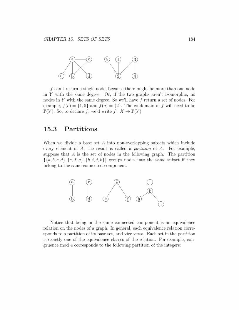
CHAPTER 15. SETS OF SETS 184
a
b
c
de
5 1
2
3
4
f can’t return a single node, because there might be more than one nodein Y with the same degree. Or, if the two graphs aren’t isomorphic, nonodes in Y with the same degree. So we’ll have f return a set of nodes. Forexample, f(e) = {1, 5} and f(a) = {2}. The co-domain of f will need to beP(Y ). So, to declare f , we’d write f : X → P(Y ).
15.3 Partitions
When we divide a base set A into non-overlapping subsets which includeevery element of A, the result is called a partition of A. For example,suppose that A is the set of nodes in the following graph. The partition{{a, b, c, d}, {e, f, g}, {h, i, j, k}} groups nodes into the same subset if theybelong to the same connected component.
a
b
c
d e f
g
hi
j
k
Notice that being in the same connected component is an equivalencerelation on the nodes of a graph. In general, each equivalence relation corre-sponds to a partition of its base set, and vice versa. Each set in the partitionis exactly one of the equivalence classes of the relation. For example, con-gruence mod 4 corresponds to the following partition of the integers:
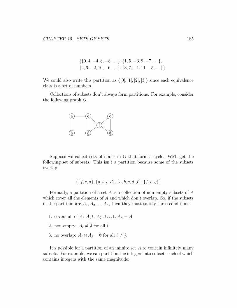
CHAPTER 15. SETS OF SETS 185
{{0, 4,−4, 8,−8, . . .}, {1, 5,−3, 9,−7, . . .},{2, 6,−2, 10,−6, . . .}, {3, 7,−1, 11,−5, . . .}}
We could also write this partition as {[0], [1], [2], [3]} since each equivalenceclass is a set of numbers.
Collections of subsets don’t always form partitions. For example, considerthe following graph G.
a
b
c
d
f
e
g
Suppose we collect sets of nodes in G that form a cycle. We’ll get thefollowing set of subsets. This isn’t a partition because some of the subsetsoverlap.
{{f, c, d}, {a, b, c, d}, {a, b, c, d, f}, {f, e, g}}
Formally, a partition of a set A is a collection of non-empty subsets of Awhich cover all the elements of A and which don’t overlap. So, if the subsetsin the partition are A1, A2, . . . An, then they must satisfy three conditions:
1. covers all of A: A1 ∪ A2 ∪ . . . ∪ An = A
2. non-empty: Ai 6= ∅ for all i
3. no overlap: Ai ∩ Aj = ∅ for all i 6= j.
It’s possible for a partition of an infinite set A to contain infinitely manysubsets. For example, we can partition the integers into subsets each of whichcontains integers with the same magnitude:
CHAPTER 15. SETS OF SETS 186
{{0}, {1,−1}, {2,−2}, {3,−3}, . . .}
We need more general notation to cover the possibility of an infinitepartition. Suppose that P is a partition of A. Then P must satisfy thefollowing conditions:
1. covers all of A:⋃
X∈P X = A
2. non-empty: X 6= ∅ for all X ∈ P
3. no overlap: X ∩ Y = ∅ for all X, Y ∈ P , X 6= Y
The three defining conditions of an equivalence relation (reflexive, sym-metric, and transitive) were chosen so as to force the equivalence classesto be a partition. Relations without one of these properties would gener-ate “equivalence classes” that might be empty, have partial overlaps, and soforth.
15.4 Combinations
In many applications, we have an n-element set and need to count all subsetsof a particular size k. A subset of size k is called a k-combination. Noticethe difference between a permutation and a combination: we care about theorder of elements in a permutation but not in a combination.
For example, how many ways can I select a 7-card hand from a 60-carddeck of Magic cards (assuming no two cards are identical)?1
One way to analyze this problem is to figure out how many ways wecan select an ordered list of 7 cards, which is P (60, 7). This over-counts thenumber of possibilities, so we have to divide by the number of different ordersin which the same 7-cards might appear. That’s just 7!. So our total number
1Ok, ok, for those of you who actually play Magic, decks do tend to contain identical
land cards. But maybe we are using lots of special lands or perhaps we’ll treat cards with
different artwork as different.

CHAPTER 15. SETS OF SETS 187
of hands is P (60,7)7!
This is 60·59·58·57·56·55·547·6·5·4·3·2
. Probably not worth simplifying ormultiplying this out unless you really have to. (Get a computer to do it.)
In general, suppose that we have a set S with n elements and we want tochoose an unordered subset of k elements. We have n!
(n−k)!ways to choose k
elements in some particular order. Since there are k! ways to put each subsetinto an order, we need to divide by k! so that we will only count each subsetonce. So the general formula for the number of possible subsets is n!
k!(n−k)!.
The expression n!k!(n−k)!
is often written C(n, k) or(
n
k
)
. This is pronounced“n choose r.” It is also sometimes called a “binomial coefficient,” for reasonsthat will become obvious shortly. So the shorthand answer to our questionabout magic cards would be
(
607
)
.
Notice that(
n
r
)
is only defined when n ≥ r ≥ 0. What is(
00
)
? This is0!0!0!
= 11·1
= 1.
15.5 Applying the combinations formula
The combinations formula is often used when we want to select a set oflocations or positions to contain a specific value. For example, suppose wewant to figure out how many 16-digit bit strings contain exactly 5 zeros.Let’s think of the string as having 16 positions. We need to choose 5 of theseto be the positions containing the zeros. We can how apply the combinationsformula: we have
(
165
)
ways to select these 5 positions.
To take a slightly harder example, let’s figure out how many 10-characterstrings from the 26-letter ASCII alphabet contain no more than 3 A’s. Suchstrings have to contain 0, 1, 2, or 3 A’s. To find the number of stringscontaining exactly three A’s, we first pick three of the 10 positions to containthe A’s. There are
(
103
)
ways to do this. Then, we have seven positions to fillwith our choice of any character except A. We have 257 ways to do that. Soour total number of strings with 3 A’s is
(
103
)
257.
To get the total number of strings, we do a similar analysis to countthe strings with 0, 1, and 2 A’s. We then add up the counts for the fourpossibilities to get a somewhat messy final answer for the number of stringswith no 3 or fewer A’s:

CHAPTER 15. SETS OF SETS 188
(
103
)
257 +(
102
)
258 +(
101
)
259 + 2510
15.6 Combinations with repetition
Suppose I have a set S and I want to select a group of objects of the typeslisted in S, but I’m allowed to pick more than one of each type of object.For example, suppose I want to pick 6 plants for my garden and the set ofavailable plants is S = {thyme, oregano,mint}. The garden store can supplyas many as I want of any type of plant. I could pick 3 thyme and 3 mint. OrI could pick 2 thyme, 1 oregano, and 3 mint.
There’s a clever way to count the possibilities here. Let’s draw a picture ofa selection as follows. We’ll group all our thymes together, then our oreganos,then our mints. Between each pair of groups, we’ll put a cardboard separator#. So 2 thyme, 1 oregano, and 3 mint looks like
T T # O # M M M
And 3 thyme and 3 mint looks like
T T T ## M M M
But this picture is redundant, since the items before the first separatorare always thymes, the ones between the separators are oreganos, and thelast group are mints. So we can simplify the diagram by using a star for eachobject and remembering their types implicitly. Then 2 thyme, 1 oregano,and 3 mint looks like
** # * # ***
And 3 thyme and 3 mint looks like
*** ## ***

CHAPTER 15. SETS OF SETS 189
To count these pictures, we need to count the number of ways to arrange6 stars and two #’s. That is, we have 8 positions and need to choose 2 to fill
with #’s. In other words,
(
82
)
.
In general, suppose we are picking a group of k objects (with possibleduplicates) from a list of n types. Then our picture will contain k stars andn− 1 #’s. So we have k + n− 1 positions in the picture and need to choosen − 1 positions to contain the #’s. So the number of possible pictures is(
k + n− 1n− 1
)
.
Notice that this is equal to
(
k + n− 1k
)
because we have an identity
that says so (see above). We could have done our counting by picking asubset of k positions in the diagram that we would fill with stars (and thenthe rest of the positions will get the #’s).
If wanted to pick 20 plants and there were five types available, I would
have
(
244
)
=
(
2420
)
options for how to make my selection.
(
244
)
=
24·23·22·214·3·3
= 23 · 22 · 21.
15.7 Identities for binomial coefficients
There are a large number of useful identities involving binomial coefficients,most of which you can look up as you need them. Two really basic ones areworth memorizing. First, a simple consequence of the definition of
(
n
k
)
is that
(
n
k
)
=
(
n
n− k
)
Pascal’s identity also shows up frequently. It states that
(Pascal’s identity)(
n+1k
)
=(
n
k
)
+(
n
k−1
)
This is not hard to prove from the definition of(
n
k
)
. To remember it, suppose

CHAPTER 15. SETS OF SETS 190
that S is a set with n+ 1 elements. The lefthand side of the equation is thenumber of k-element subsets of S.
Now, fix some element a in S. There are two kinds of k-element subsets:(1) those that don’t contain a and (2) those that do contain a. The first termon the righthand side counts the subsets in group (1): all k-element subsetsof S −{a}. The second term on the righthand side counts the k− 1-elementsubsets of S − {a}. We then add a to each of these to get the subsets ingroup (2).
If we have Pascal’s identity, we can give a recursive definition for thebinomial coefficients, for all natural numbers n and k with k ≤ n.
Base: For any natural number k,(
n
0
)
=(
n
n
)
= 1.
Induction:(
n
k
)
=(
n−1k−1
)
+(
n−1k
)
, whenever k < n
15.8 Binomial Theorem
Remember that a binomial is a sum of two terms, e.g. (x + y). Binomialcoefficients get their name from the following useful theorem about raising abinomial to an integer power:
Claim 54 (Binomial Theorem) Let x and y be variables and let n be anynatural number. Then
(x+ y)n =
n∑
k=0
(
n
k
)
xn−kyk
When we expand the product (x + y)n, each term is the product of nvariables, some x’s and the rest y’s. For example, if n = 5, one term isyxyyx. So each term is an ordered list of x’s and y’s.
We can think of our large set of terms as partitioned into subsets, eachcontaining terms with the same number of x’s. For example, the set of termswith two x’s would be
CHAPTER 15. SETS OF SETS 191
[xxyyy] = {xxyyy, xyxyy, xyyxy, xyyyx, yxxyy,yxyxy, yxyyx, yyxxy, yyxyx, yyyxx}
When we collect terms, the coefficient for each term will be the size of thisset of equivalent terms. E.g. the coefficient for x2y3 is 10, because [xxyyy]contains 10 elements. To find the coefficient for xn−kyk, we need to counthow many ways we can make a sequence of n variable names that containsk y’s and n− k x’s. This amounts to picking a subset of k elements from aset of n positions in the sequence. In other words, there are
(
n
k
)
such terms.
15.9 Variation in notation
We’ve used the notation P(A) for the powerset of A. Another commonnotation is 2A.
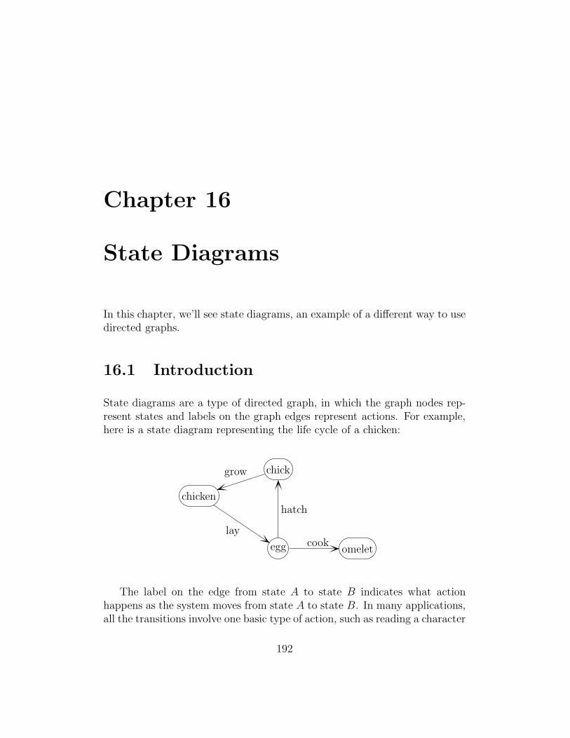
Chapter 16
State Diagrams
In this chapter, we’ll see state diagrams, an example of a different way to usedirected graphs.
16.1 Introduction
State diagrams are a type of directed graph, in which the graph nodes rep-resent states and labels on the graph edges represent actions. For example,here is a state diagram representing the life cycle of a chicken:
chicken
egg
chick
omelet
hatch
grow
laycook
The label on the edge from state A to state B indicates what actionhappens as the system moves from state A to state B. In many applications,all the transitions involve one basic type of action, such as reading a character
192
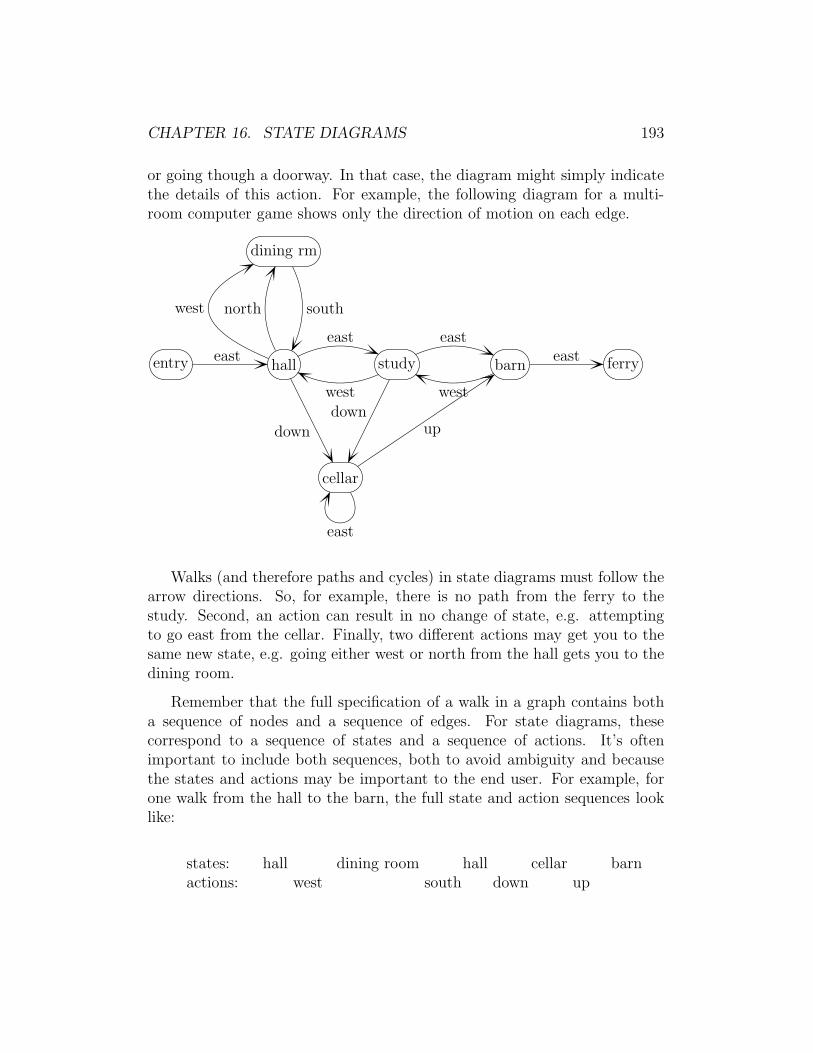
CHAPTER 16. STATE DIAGRAMS 193
or going though a doorway. In that case, the diagram might simply indicatethe details of this action. For example, the following diagram for a multi-room computer game shows only the direction of motion on each edge.
entry
dining rm
hall study barn ferry
cellar
northwest south
easteast
west
east
west
east
down
downup
east
Walks (and therefore paths and cycles) in state diagrams must follow thearrow directions. So, for example, there is no path from the ferry to thestudy. Second, an action can result in no change of state, e.g. attemptingto go east from the cellar. Finally, two different actions may get you to thesame new state, e.g. going either west or north from the hall gets you to thedining room.
Remember that the full specification of a walk in a graph contains botha sequence of nodes and a sequence of edges. For state diagrams, thesecorrespond to a sequence of states and a sequence of actions. It’s oftenimportant to include both sequences, both to avoid ambiguity and becausethe states and actions may be important to the end user. For example, forone walk from the hall to the barn, the full state and action sequences looklike:
states: hall dining room hall cellar barnactions: west south down up

CHAPTER 16. STATE DIAGRAMS 194
16.2 Wolf-goat-cabbage puzzle
State diagrams are often used to model puzzles or games. For example, onefamous puzzle involves a farmer taking a wolf, a goat, and a cabbage tomarket. To do this, he must cross from the east to the west side of a riverusing a boat that can only carry him plus one of his three possessions. Hecannot leave the wolf and goat together unsupervised, nor the goat and thecabbage, because one will eat the other.
We can represent each state of this system by listing the objects that areon the east bank: w is the wolf, g is the goat, c is the cabbage, and b is theboat. States like wc and wgb are legal, but wg would not be a legal state.The diagram of legal states then looks as follows:
wgcb wc wcb
w
c
wgb
cgb
g gb ∅
In this diagram, actions aren’t marked on the edges: you’re left to inferthe action from the change in state. The start state (wgcb) where the systembegins is marked by showing an error leading into it. The end state (∅) wherenothing is left on the east bank is marked with a double ring.
In this diagram, it is possible for a (directed) walk to loop back on itself,repeating states. So there are an infinite number of solutions to this puzzle.
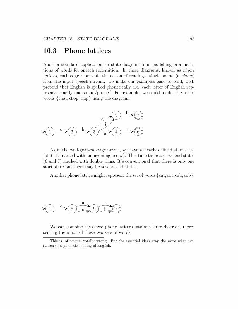
CHAPTER 16. STATE DIAGRAMS 195
16.3 Phone lattices
Another standard application for state diagrams is in modelling pronuncia-tions of words for speech recognition. In these diagrams, known as phonelattices, each edge represents the action of reading a single sound (a phone)from the input speech stream. To make our examples easy to read, we’llpretend that English is spelled phonetically, i.e. each letter of English rep-resents exactly one sound/phone.1 For example, we could model the set ofwords {chat, chop, chip} using the diagram:
1 2 3 4
5
6
7
c ha
t
oi
p
As in the wolf-goat-cabbage puzzle, we have a clearly defined start state(state 1, marked with an incoming arrow). This time there are two end states(6 and 7) marked with double rings. It’s conventional that there is only onestart state but there may be several end states.
Another phone lattice might represent the set of words {cat, cot, cab, cob}.
1 8 9 10c
a
o
t
b
We can combine these two phone lattices into one large diagram, repre-senting the union of these two sets of words:
1This is, of course, totally wrong. But the essential ideas stay the same when you
switch to a phonetic spelling of English.
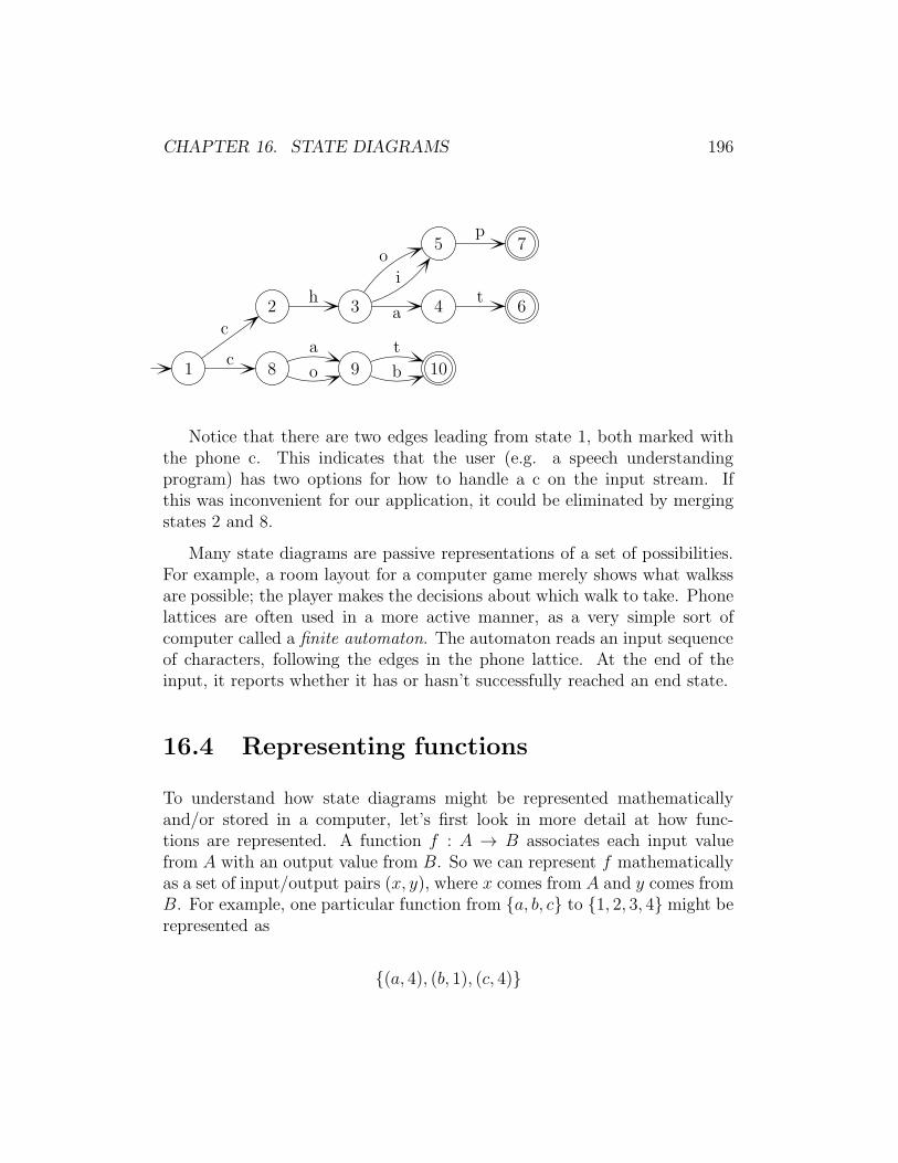
CHAPTER 16. STATE DIAGRAMS 196
1
2 3 4
5
6
7
8 9 10c
a
o
t
b
c
ha
t
oi
p
Notice that there are two edges leading from state 1, both marked withthe phone c. This indicates that the user (e.g. a speech understandingprogram) has two options for how to handle a c on the input stream. Ifthis was inconvenient for our application, it could be eliminated by mergingstates 2 and 8.
Many state diagrams are passive representations of a set of possibilities.For example, a room layout for a computer game merely shows what walkssare possible; the player makes the decisions about which walk to take. Phonelattices are often used in a more active manner, as a very simple sort ofcomputer called a finite automaton. The automaton reads an input sequenceof characters, following the edges in the phone lattice. At the end of theinput, it reports whether it has or hasn’t successfully reached an end state.
16.4 Representing functions
To understand how state diagrams might be represented mathematicallyand/or stored in a computer, let’s first look in more detail at how func-tions are represented. A function f : A → B associates each input valuefrom A with an output value from B. So we can represent f mathematicallyas a set of input/output pairs (x, y), where x comes from A and y comes fromB. For example, one particular function from {a, b, c} to {1, 2, 3, 4} might berepresented as
{(a, 4), (b, 1), (c, 4)}

CHAPTER 16. STATE DIAGRAMS 197
In a computer, this information might be stored as a linked list of pairs.Each pair might be a short list, or an object or structure. However, findinga pair in such a list requires time proportional to the length of the list. Thiscan be very slow if the list is long i.e. if the domain of the function is large.
Another option is to convert input values to small integers. For example,in C, lowercase integer values (as in the set A above) can be converted to smallintegers by subtracting 97 (the ASCII code for a). We can then store thefunction’s input/output pairs using an array. Each array position representsan input value. Each array cell contains the corresponding output value.
16.5 Transition functions
Formally, we can define a state diagram to consist of a set of states S, a set ofactions A, and a transition function δ that maps out the edges of the graph,i.e. shows how actions result in state changes. Each edge of the state diagramshows what happens when you are in a particular state s and execute someaction a, i.e. which new state(s) could you be in.
So an input to δ is a pair (s, a) of a state and an action. In some appli-cations, there is only exactly one new state that could result from applyingaction a in state s. For those applications, we can give δ the type signatureδ : S × A → S.
However, in some state diagrams, it might not be possible to executecertain actions from certain states. E.g. you can’t go up from the study inour room layout example. And, as we saw in the phone lattice example, itis sometimes convenient to allow the user or the computer system severalchoices for the new state. When we need to support these possibilities, eachoutput of δ must be a set of states. So the type signature of δ must look likeδ : S × A → P(S).
The hard part of implementing state diagrams in a computer programis storing the transition function. We could build a 2D array, whose cellsrepresent all the pairs (s, a). Each cell would then contain a list of outputstates. This wouldn’t be very efficient, however, because state diagrams tendto be sparse: most state/action pairs don’t produce any new state.

CHAPTER 16. STATE DIAGRAMS 198
One better approach is to build a 1D array of states. The cell for eachstate contains a list of actions possible from that state, together with thenew states for each action. For example, in our final phone lattice, theentry for state 1 would be ((c, (2, 8))) and the entry for state 3 would be((o, (5)), (i, (5)), (a, (4))). This adjacency list style of storage is much morecompact, because we are no longer wasting space representing the large num-ber of impossible actions.
Another approach is to build a function, called a hash function that mapseach state/action pair to a small integer. We then allocate a 1D array withone position for each state/action pair. Each array cell then contains a listof new states for this state/action pair. The details of hash functions arebeyond the scope of this class. However, modern programming languagesoften include built-in hash table or dictionary objects that handle the detailsfor you.
16.6 Shared states
Suppose that each word in our dictionary had its own phone lattice, andwe then merge these individual lattices to form lattices representing sets ofwords. We might get a lattice like the following one, which represents theset of words {cop, cap, cops, caps}.
1 5 6 7 8
2 3 4
9 10 11 12
13 14 15
c a p sc
a p
co p sc
o p
Although this lattice encodes the right set of words, it uses a lot morestates than necessary. We can represent the same information using thefollowing, much more compact, phone lattice.
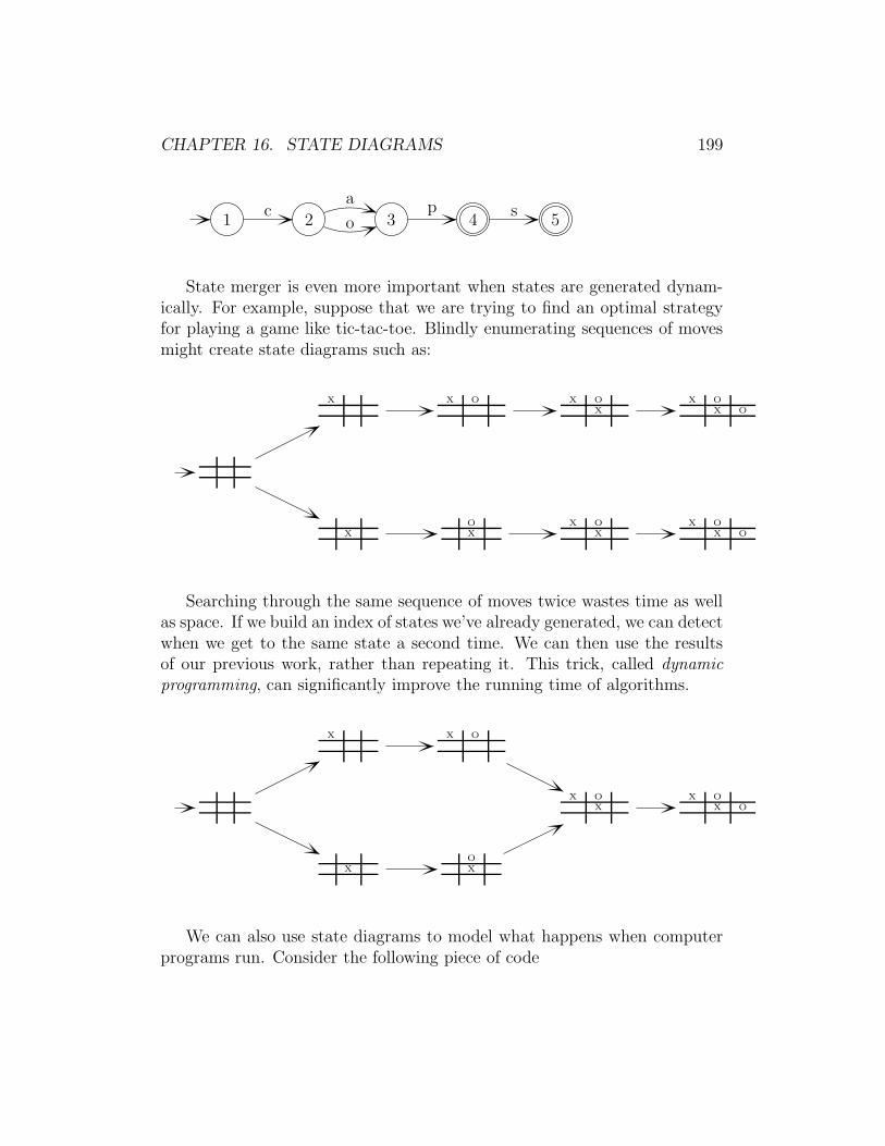
CHAPTER 16. STATE DIAGRAMS 199
1 2 3 4 5c
a
op s
State merger is even more important when states are generated dynam-ically. For example, suppose that we are trying to find an optimal strategyfor playing a game like tic-tac-toe. Blindly enumerating sequences of movesmight create state diagrams such as:
X
X
O
X
X O
X O
X
X O
X
X O
X O
X O
X O
Searching through the same sequence of moves twice wastes time as wellas space. If we build an index of states we’ve already generated, we can detectwhen we get to the same state a second time. We can then use the resultsof our previous work, rather than repeating it. This trick, called dynamicprogramming, can significantly improve the running time of algorithms.
X
X
O
X
X O
X O
X
X O
X O
We can also use state diagrams to model what happens when computerprograms run. Consider the following piece of code
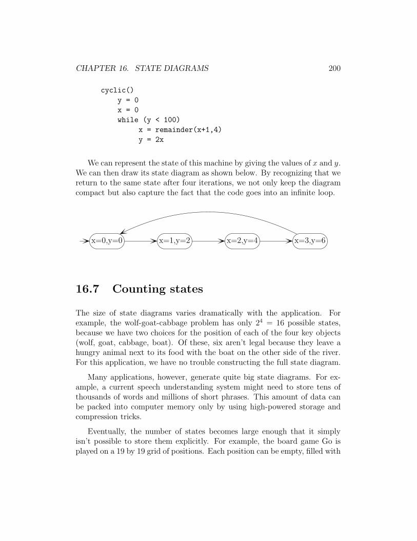
CHAPTER 16. STATE DIAGRAMS 200
cyclic()
y = 0
x = 0
while (y < 100)
x = remainder(x+1,4)
y = 2x
We can represent the state of this machine by giving the values of x and y.We can then draw its state diagram as shown below. By recognizing that wereturn to the same state after four iterations, we not only keep the diagramcompact but also capture the fact that the code goes into an infinite loop.
x=0,y=0 x=1,y=2 x=2,y=4 x=3,y=6
16.7 Counting states
The size of state diagrams varies dramatically with the application. Forexample, the wolf-goat-cabbage problem has only 24 = 16 possible states,because we have two choices for the position of each of the four key objects(wolf, goat, cabbage, boat). Of these, six aren’t legal because they leave ahungry animal next to its food with the boat on the other side of the river.For this application, we have no trouble constructing the full state diagram.
Many applications, however, generate quite big state diagrams. For ex-ample, a current speech understanding system might need to store tens ofthousands of words and millions of short phrases. This amount of data canbe packed into computer memory only by using high-powered storage andcompression tricks.
Eventually, the number of states becomes large enough that it simplyisn’t possible to store them explicitly. For example, the board game Go isplayed on a 19 by 19 grid of positions. Each position can be empty, filled with

CHAPTER 16. STATE DIAGRAMS 201
a black stone, or filled with a white stone. So, to a first approximation, wehave 3361 possible game positions. Some of these are forbidden by the rulesof the game, but not enough to make the size of the state space tractable.
Some games and theoretical models of computation use an unboundedamount of memory, so that their state space becomes infinite. For example,Conway’s “Game of Life” runs on an 2D grid of cells, in which each cell has8 neighbors. The game starts with an initial configuration, in which someset of cells is marked as live, and the rest are marked as dead. At each timestep, the set of live cells is updated using the rules:
• A live cell stays live if it 2 or 3 neighbors. Otherwise it becomes dead.
• A dead cell with exactly 3 neighbors becomes live.
For some initial configurations, the system goes into a stable state oroscillates between several configurations. However, even if the initial set oflive cells is finite, the set of live cells can grow without bound as time movesforwards. So, for some initial configurations, the system has infinitely manystates.
When a system has an intractably large number of states, whether finiteor infinite, we obviously aren’t going to build its state space explicitly. Anal-ysis of such systems requires techniques like computing high-level propertiesof states, generating states in a smart way, and using heuristics to decidewhether a state is likely to lead to a final solution.
16.8 Variation in notation
State diagrams of various sorts, and constructs very similar to state diagrams,are used in a wide range of applications. Therefore, there are many differentsets of terminology for equivalent and/or subtly different variations on thisidea. In particular, when a state diagram is viewed as an active device, i.e.as a type of machine or computer, it is often called a state transition or anautomaton.
Start states are also known as initial states. End states can be called endstates or goal states.
Chapter 17
Countability
This chapter covers infinite sets and countability.
17.1 The rationals and the reals
You’re familiar with three basic sets of numbers: the integers, the rationals,and the reals. The integers are obviously discrete, in that there’s a big gapbetween successive pairs of integers.
To a first approximation, the rational numbers and the real numbers seempretty similar. The rationals are dense in the reals: if I pick any real numberx and a distance δ, there is always a rational number within distance δ of x.Between any two real numbers, there is always a rational number.
We know that the reals and the rationals are different sets, because we’veshown that a few special numbers are not rational, e.g. π and
√2. However,
these irrational numbers seem like isolated cases. In fact, this intuition isentirely wrong: the vast majority of real numbers are irrational and therationals are quite a small subset of the reals.
202
CHAPTER 17. COUNTABILITY 203
17.2 Completeness
One big difference between the two sets is that the reals have a so-called“completeness” property. It states that any subset of the reals with an upperbound has a smallest upper bound. (And similarly for lower bounds.) So if Ihave a sequence of reals that converges, the limit it converges to is also a realnumber. This isn’t true for the rationals. We can make a series of rationalnumbers that converge π (for example) such as
3, 3.1, 3.14, 3.141, 3.1415, 3.14159, 3.141592, 3.1415926, 3.14159265
But there is no rational number equal to π.
In fact, the reals are set up precisely to make completeness work. Oneway to construct the reals is to construct all convergent sequences of rationalsand add new points to represent the limits of these sequences. Most of themachinery of calculus depends on the existence of these extra points.
17.3 Cardinality
We know how to calculate and compare the sizes of finite sets. To extendthis idea to infinite sets, we use bijections functions to compare the sizes ofsets:
Definition: Two sets A and B have the same cardinality (|A| =|B|) if and only if there is a bijection from A to B.
We’ve seen that there is a bijection between two finite sets exactly whenthe sets have the same number of elements. So this definition of cardinalitymatches our normal notion of how big a finite set is. But, since we don’thave any numbers of infinite size, working with bijections extends better toinfinite sets.
The integers and the natural numbers have the same cardinality, becausewe can construct a bijection between them. Consider the function f : N → Z
where f(n) = n2when n is even and f(n) = −(n+1)
2when n is odd. f maps

CHAPTER 17. COUNTABILITY 204
the even natural numbers bijectively onto the non-negative integers. It mapsthe odd natural numbers bijectively onto the negative integers.
Because the integers are so important, there’s a special name for sets thathave the same cardinality as the integers:
An infinite set A is countably infinite if there is a bijection fromN (or equivalently Z) onto A.
The term countable is used to cover both finite sets and sets that are count-ably infinite.
17.4 More countably infinite sets
Now, let’s look at N2, the set of pairs of natural numbers. This set is count-ably infinite, because we can construct a bijection f : N2 → N. To do this,we’ll organize the set of pairs of natural numbers by size, where the size of apair (p, q) is the sum p+ q of its coordinates. The pairs of size k are mapped
onto an interval of length k + 1 starting at k(k+1)2
. You can verify that theseintervals cover the natural numbers exactly, without overlapping. Withineach interval, we map pairs to integer positions in order, based on the sizeof the first coordinate p. This map is a bijection from the pairs of naturalnumbers to the natural numbers.
Suppose that we have a finite set A of n characters. Then the set A∗
contains all finite sequences of characters from A. For example, A might bethe set of ASCII characters. In that case, A∗ contains character strings ofvarious finite lengths, such as “a,” “This,” and “transitivity.” A∗ is countablyinfinite. Again, we organize these strings by size, but this time “size” is thelength of the strings. The nk strings of length k are mapped into an intervalof the integers, starting right after the interval for the strings of length k−1.If you work out the coordinates properly, this also ends up as a bijection.
These constructions can be extended to show the countability of a varietyof similar sets, e.g. positive integers, triples of natural numbers, or 7-tuplesof integers.
CHAPTER 17. COUNTABILITY 205
17.5 Cantor Schroeder Bernstein Theorem
For certain countably infinite sets, it’s awkward to directly build a bijectionto the integers or natural numbers. Fortunately, a more general technique isavailable. Remember that for finite sets, we could build a one-to-one functionfrom A to B if and only if |A| ≤ |B|. Using this idea, we can define a partialorder on sets, finite or infinite:
Definition: |A| ≤ |B| if and only if there is a one-to-one functionfrom A to B.
It is the case that if |A| ≤ |B| and |B| ≤ |A|, then |A| = |B|. That is, ifyou can build one-to-one functions in both directions, a bijection does exist.This result, called the Cantor Schroeder Bernstein Theorem, isn’t obviouswhen the sets are infinite. You do have enough background to understandits proof (which you can look up), but it’s somewhat messy.
To see this theorem in action, consider the rational numbers. Rationalnumbers are almost the same as fractions, which are basically pairs of in-tegers, which we know to be countablily infinite. But this isn’t quite right:each rational number is represented by many fractions.
So, let’s use Cantor Schroeder Bernstein: to show that the positive ratio-nal numbers are the same size as the natural numbers show that |N| ≤ |Q+|and |Q+| ≤ |N|. It’s easy to make a one-to-one function from the naturalnumbers to the positive rational numbers: just map each natural number nto n + 1 (because Q+ doesn’t include zero). So |N| ≤ |Q+|. So now we justneed a one-to-one function from the rationals to the integers, to show that|Q+| ≤ |N|.
To map the positive rational numbers to the natural numbers, first mapeach rational number to one representative fraction, e.g. the one in lowestterms. This isn’t a bijection, but it is one-to-one. Then use the method wesaw above to map the fractions, which are just pairs of positive integers, tothe natural numbers. We now have the required one-to-one function fromthe positive rationals to the natural numbers.
Again, this construction can be adapted to also handle negative rationalnumbers. So the set of rational numbers is countably infinite.

CHAPTER 17. COUNTABILITY 206
17.6 P(N) isn’t countable
Before looking at the real numbers, let’s first prove a closely-related resultthat’s less messy: P(N) isn’t countable. Recall that P(N) is the power set ofthe natural numbers i.e. the set containing all subsets of the natural numbers.
Suppose that A is a finite set {a0, a1, a2, . . . , an}. We can represent asubset X of A as a bit vector {b0, b1, b2, . . . , bn} where bi is 1 if and only ifai is in X . For example, if A = {7, 8, 9, 10, 11}, then the bit-vector 01100would represent the subset {8, 9} and the bit-vector 10101 would representthe subset {7, 9, 11}. Similarly, we can represent a subset of the naturalnumbers as an infinite-length bit vector.
We’ll use a procedure called “diagonalization” (due to Georg Cantor) toshow that it’s impossible to build a bijection from the natural numbers tothese infinite bit vectors representing the subsets of the natural numbersSuppose that there were such a bijection. Then we could put all the bitvectors into a list, e.g. v0 would be the first bit vector, v1 the second, andso forth. Our list of bit vectors might look like this, where the kth columncontains the value of the kth digit (bk) for all the bit vectors:
b0 b1 b2 b3 b4 b5 b6 b7 b8 b9 . . .
v0 1 1 0 1 1 0 1 1 1 1 . . .v1 1 1 0 0 1 0 1 1 0 0 . . .v2 0 0 0 0 1 0 0 1 0 0 . . .v3 0 1 1 1 1 0 1 0 0 0 . . .v4 0 0 0 0 1 1 1 0 1 1 . . .v5 1 1 1 0 1 0 1 0 0 1 . . .. . . . . .
This is supposed to be a complete list of all the bit vectors. But we canconstruct a bit vector x that’s not on the list. The value of xk, i.e. the kthbit in our new vector, will be 0 if the k digit of vk is 1, and 1 if the k digitof vk is 0. Notice that x is different from v3 because the two vectors differin the third position. It can’t be v20 because the two vectors differ in thetwentieth position. And, in general, x can’t equal vk because the two vectorsdiffer in the kth position. For the example above, the new vector not in thelist would start out: 0 0 1 0 0 1 . . ..
CHAPTER 17. COUNTABILITY 207
So, it’s not possible to put these infinite bit vectors into a list indexedby the natural numbers, because we can always construct a new bit vectorthat’s not on the list. That is, there can’t be a one-to-one function from theinfinite bit vectors to the natural numbers. So there can’t be a one-to-onefunction from the subsets of the natural numbers to the natural numbers. SoP(N) isn’t countable. That is, the subsets of the natural numbers are morenumerous than the natural numbers themselves.
17.7 More uncountability results
This same diagonalization trick can be used to show that various other setsaren’t countable. For example, we can show that the real numbers aren’tcountable. To show this, we show that even the numbers in the interval[0, 1] aren’t countable. Suppose that the elements of [0, 1] were countable.Then we could put these real numbers into a list a1, a2, and so forth. Let’swrite out a table of the decimal expansions of the numbers on this list. Now,examine the digits along the diagonal of this table: a11, a22, etc. Supposewe construct a new number b whose kth digit bk is 4 when akk is 5, and 5otherwise. Then b won’t match any of the numbers in our table, so our tablewasn’t a complete list of all the numbers in [0, 1]. So, [0, 1] is not countable,and therefore the reals can’t be countable.
Next, notice that an infinite bit vector is a function from the naturalnumbers to the set {0, 1}. So we’ve shown that there are uncountably manyfunctions from the natural numbers to {0, 1}. So there must be uncountablymany functions from the natural numbers to the natural numbers, or fromthe integers to the integers.
Another generalization involves noticing that our diagonalization proofdoesn’t really depend on any special properties of the natural numbers. Soit can be adapted to show that, if A is any set, P(A) has a (strictly) largercardinality thanA. So, not only is P(N) larger than P(N), but P(P(N)) is evenlarger. So there is a whole sequence of larger and larger infinite cardinalities.
So, in particular, P(R) is larger than R). However, notice that R2 has thesame cardinality as R. Let’s consider a simpler version of this problem: [0, 1)2
has the same cardinality as [0, 1). Any element of [0, 1)2 can be represented
CHAPTER 17. COUNTABILITY 208
as two infinite sequences of decimal digits: 0.a1a2a3a4 . . . and 0.b1b2b3b4 . . ..We can map this to a single real number by interleaving the digits of the twonumbers: 0.a1b1a2b2a3b3 . . .. This defines a bijection between the two sets.This method can be adapted to create a bijection between all of R2 and R.
17.8 Uncomputability
We can pull some of these facts together into some interesting consequencesfor computer science. Notice that a formula for a function is just a finitestring of characters. So the set of formulas is countable. But the set offunctions, even from the integers to the integers, is uncountable. So thereare more functions than formulas, i.e. some functions which have no finiteformula.
Similarly, notice that a computer program is simply a finite string ofASCII characters. So there are only countably many computer programs.But there are uncountably many functions. So there are more functionsthan programs, i.e. there are functions which cannot be computed by anyprogram.
A final problem is created by the fact that, although the code for a com-puter program is finite in length, the trace of the program’s execution maybe infinite. Specifically, program traces fall into three categories
(1) The program eventually halts, so the trace is finite.
(2) The program loops, in the sense of returning back to a previous state.
(3) The program keeps going forever, consuming more and more storagespace.
The second type of behavior is like the decimal expansion of a rationalnumber: repeating. This third type of behavior is similar to a real number’sdecimal expansion: an infinite sequence which doesn’t repeat. As with num-bers, the infinite non-repeating sequences create interesting complexity. Inthis case, the famous Halting Problem which shows that you can’t build aprogram that will decide whether other programs halt or not.
CHAPTER 17. COUNTABILITY 209
A final example, further afield but closely related mathematically, involvestilings of the plane. Periodic tilings, which are made up of many copies of asingle repeated pattern, are like rational numbers or looping programs. Ape-riodic tilings, whose existence was only proved in 1966, are like real numbersor the third type of program: they go on forever, but not by repeating a sin-gle pattern over and over. See the internet for pictures of aperiodic tilings,especially Penrose tilings. Aside from looking cool, they have applications inmodelling “quasicrystals” e.g. you can create a crystal-like structures with a5-fold symmetry.
17.9 Variation in notation
Authors differ as to whether the term countable includes finite sets or onlycountably infinite sets.
Chapter 18
Planar Graphs
This chapter covers special properties of planar graphs.
18.1 Planar graphs
A planar graph is a graph which can be drawn in the plane without anyedges crossing. Some pictures of a planar graph might have crossing edges,but it’s possible to redraw the picture to eliminate the crossings. For example,although the usual pictures of K4 and Q3 have crossing edges, it’s easy toredraw them so that no edges cross. For example, a planar picture of Q3 isshown below. However, if you fiddle around with drawings of K3,3 or K5,there doesn’t seem to be any way to eliminate the crossings. We’ll see howto prove that these two graphs aren’t planar.
210
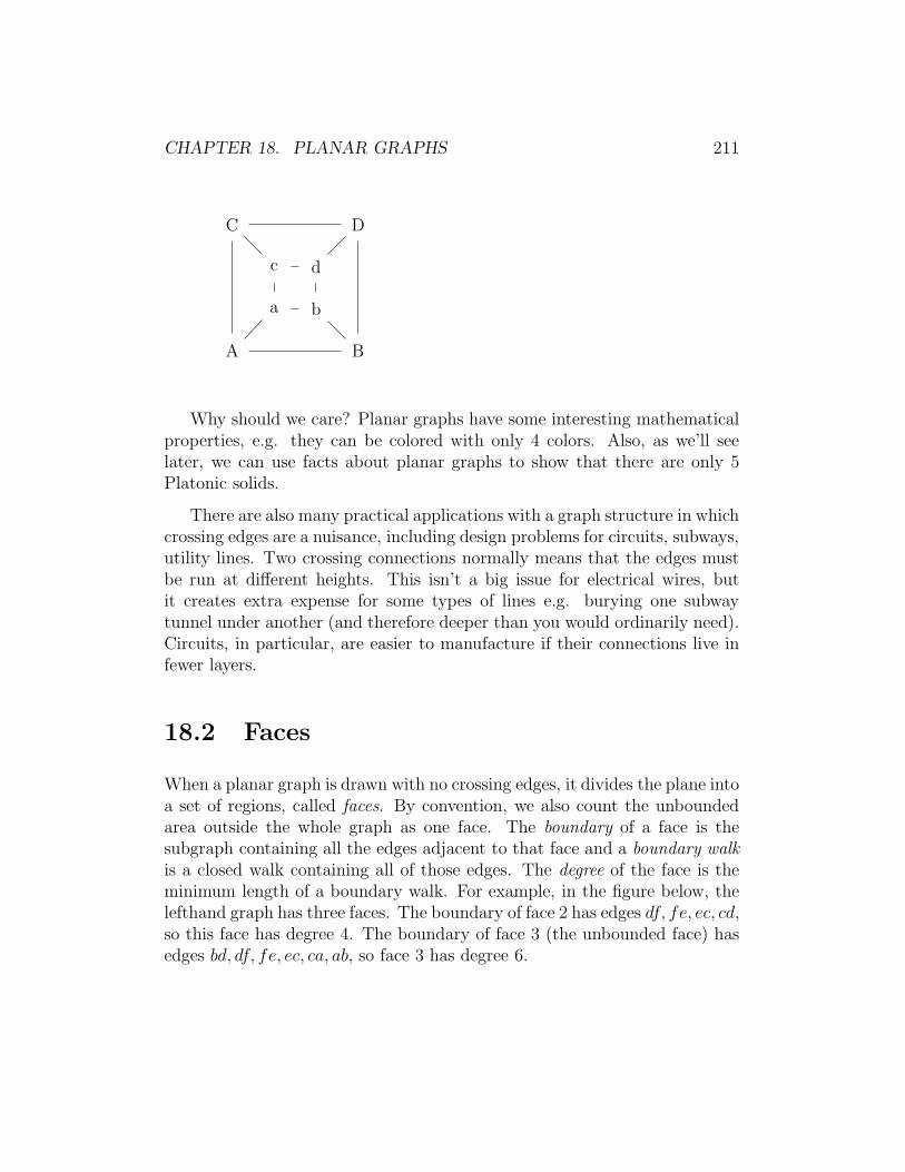
CHAPTER 18. PLANAR GRAPHS 211
a b
c d
A B
C D
Why should we care? Planar graphs have some interesting mathematicalproperties, e.g. they can be colored with only 4 colors. Also, as we’ll seelater, we can use facts about planar graphs to show that there are only 5Platonic solids.
There are also many practical applications with a graph structure in whichcrossing edges are a nuisance, including design problems for circuits, subways,utility lines. Two crossing connections normally means that the edges mustbe run at different heights. This isn’t a big issue for electrical wires, butit creates extra expense for some types of lines e.g. burying one subwaytunnel under another (and therefore deeper than you would ordinarily need).Circuits, in particular, are easier to manufacture if their connections live infewer layers.
18.2 Faces
When a planar graph is drawn with no crossing edges, it divides the plane intoa set of regions, called faces. By convention, we also count the unboundedarea outside the whole graph as one face. The boundary of a face is thesubgraph containing all the edges adjacent to that face and a boundary walkis a closed walk containing all of those edges. The degree of the face is theminimum length of a boundary walk. For example, in the figure below, thelefthand graph has three faces. The boundary of face 2 has edges df, fe, ec, cd,so this face has degree 4. The boundary of face 3 (the unbounded face) hasedges bd, df, fe, ec, ca, ab, so face 3 has degree 6.
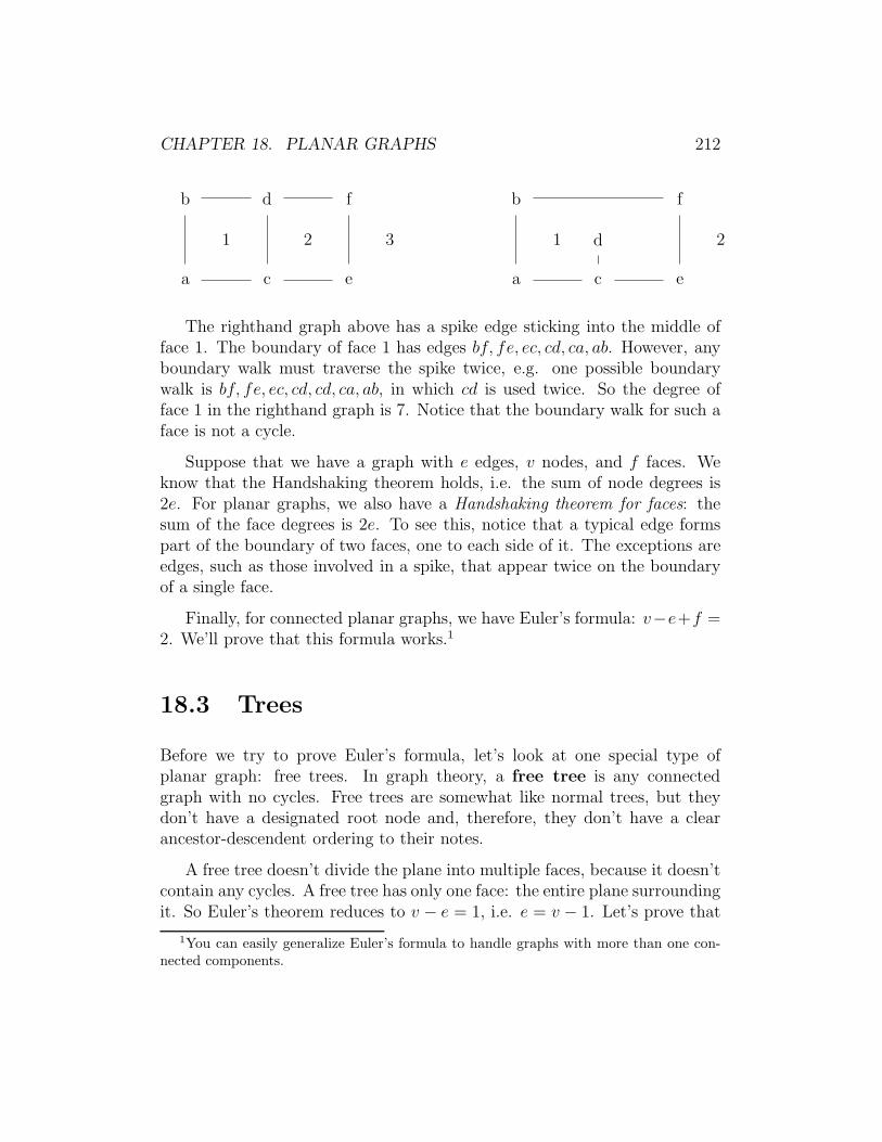
CHAPTER 18. PLANAR GRAPHS 212
1 2 3
a
b
c
d
e
f
1 2
a
b
c
d
e
f
The righthand graph above has a spike edge sticking into the middle offace 1. The boundary of face 1 has edges bf, fe, ec, cd, ca, ab. However, anyboundary walk must traverse the spike twice, e.g. one possible boundarywalk is bf, fe, ec, cd, cd, ca, ab, in which cd is used twice. So the degree offace 1 in the righthand graph is 7. Notice that the boundary walk for such aface is not a cycle.
Suppose that we have a graph with e edges, v nodes, and f faces. Weknow that the Handshaking theorem holds, i.e. the sum of node degrees is2e. For planar graphs, we also have a Handshaking theorem for faces: thesum of the face degrees is 2e. To see this, notice that a typical edge formspart of the boundary of two faces, one to each side of it. The exceptions areedges, such as those involved in a spike, that appear twice on the boundaryof a single face.
Finally, for connected planar graphs, we have Euler’s formula: v−e+f =2. We’ll prove that this formula works.1
18.3 Trees
Before we try to prove Euler’s formula, let’s look at one special type ofplanar graph: free trees. In graph theory, a free tree is any connectedgraph with no cycles. Free trees are somewhat like normal trees, but theydon’t have a designated root node and, therefore, they don’t have a clearancestor-descendent ordering to their notes.
A free tree doesn’t divide the plane into multiple faces, because it doesn’tcontain any cycles. A free tree has only one face: the entire plane surroundingit. So Euler’s theorem reduces to v − e = 1, i.e. e = v − 1. Let’s prove that
1You can easily generalize Euler’s formula to handle graphs with more than one con-
nected components.

CHAPTER 18. PLANAR GRAPHS 213
this is true, by induction.
Proof by induction on the number of nodes in the graph.
Base: If the graph contains no edges and only a single node, theformula is clearly true.
Induction: Suppose the formula works for all free trees with upto n nodes. Let T be a free tree with n + 1 nodes. We need toshow that T has n edges.
Now, we find a node with degree 1 (only one edge going into it).To do this start at any node r and follow a walk in any direction,without repeating edges. Because T has no cycles, this walk can’treturn to any node it has already visited. So it must eventuallyhit a dead end: the node at the end must have degree 1. Call itp.
Remove p and the edge coming into it, making a new free tree T ′
with n nodes. By the inductive hypothesis, T ′ has n − 1 edges.Since T has one more edge than T ′, T has n edges. Therefore ourformula holds for T .
18.4 Proof of Euler’s formula
We can now prove Euler’s formula (v − e+ f = 2) works in general, for anyconnected planar graph.
Proof: by induction on the number of edges in the graph.
Base: If e = 0, the graph consists of a single node with a singleface surrounding it. So we have 1 − 0 + 1 = 2 which is clearlyright.
Induction: Suppose the formula works for all graphs with no morethan n edges. Let G be a graph with n+ 1 edges.
Case 1: G doesn’t contain a cycle. So G is a free tree and wealready know the formula works for free trees.
CHAPTER 18. PLANAR GRAPHS 214
Case 2: G contains at least one cycle. Pick an edge p that’s on acycle. Remove p to create a new graph G′.
Since the cycle separates the plane into two faces, the faces toeither side of p must be distinct. When we remove the edge p, wemerge these two faces. So G′ has one fewer faces than G.
Since G′ has n edges, the formula works for G′ by the inductionhypothesis. That is v′ − e′ + f ′ = 2. But v′ = v, e′ = e− 1, andf ′ = f − 1. Substituting, we find that
v − (e− 1) + (f − 1) = 2
So
v − e+ f = 2
18.5 Some corollaries of Euler’s formula
Corollary 1 Suppose G is a connected planar graph, with v nodes, e edges,and f faces, where v ≥ 3. Then e ≤ 3v − 6.
Proof: The sum of the degrees of the faces is equal to twice thenumber of edges. But each face must have degree ≥ 3. So wehave 3f ≤ 2e.
Euler’s formula says that v − e + f = 2, so f = e − v + 2 andthus 3f = 3e − 3v + 6. Combining this with 3f ≤ 2e, we get3e− 3v + 6 ≤ 2e. So e ≤ 3v − 6.
We can also use this formula to show that the graph K5 isn’t planar. K5
has five nodes and 10 edges. This isn’t consistent with the formula e ≤ 3v−6.Unfortunately, this method won’t help us with K3,3, which isn’t planar butdoes satisfy this equation.
We can also use this Corollary 1 to derive a useful fact about planargraphs:

CHAPTER 18. PLANAR GRAPHS 215
Corollary 2 If G is a connected planar graph, G has a node of degree lessthan six.
Proof: This is clearly true if G has one or two nodes.
If G has at least three nodes, then suppose that the degree ofeach node was at least 6. By the handshaking theorem, 2e equalsthe sum of the degrees of the nodes, so we would have 2e ≥ 6v.But corollary 1 says that e ≤ 3v − 6, so 2e ≤ 6v − 12. We can’thave both 2e ≥ 6v and 2e ≤ 6v − 12. So there must have been anode with degree less than six.
If our graph G isn’t connected, the result still holds, because we can applyour proof to each connected component individually. So we have:
Corollary 3 If G is a planar graph, G has a node of degree less than six.
18.6 K3,3 is not planar
When all the cycles in our graph have at least four nodes, we can get a tighterrelationship between the numbers of nodes and edges.
Corollary 4 Suppose G is a connected planar graph, with v nodes, e edges,and f faces, where v ≥ 3. and if all cycles in G have length ≥ 4, thene ≤ 2v − 4.
Proof: The sum of the degrees of the faces is equal to twice thenumber of edges. But each face must have degree ≥ 4 becauseall cycles have length ≥ 4. So we have 4f ≤ 2e, so 2f ≤ e.
Euler’s formula says that v − e + f = 2, so e − v + 2 = f , so2e − 2v + 4 = 2f . Combining this with 2f ≤ e, we get that2e− 2v + 4 ≤ e. So e ≤ 2v − 4.
This result lets us show that K3,3 isn’t planar. All the cycles in K3,3 haveat least four nodes. But K3,3 has 9 edges and 6 nodes, which isn’t consistentwith this formula. So K3,3 can’t be planar.
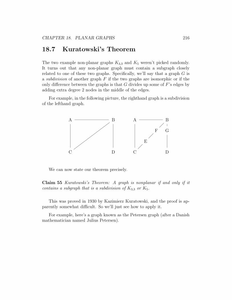
CHAPTER 18. PLANAR GRAPHS 216
18.7 Kuratowski’s Theorem
The two example non-planar graphs K3,3 and K5 weren’t picked randomly.It turns out that any non-planar graph must contain a subgraph closelyrelated to one of these two graphs. Specifically, we’ll say that a graph G isa subdivision of another graph F if the two graphs are isomorphic or if theonly difference between the graphs is that G divides up some of F ’s edges byadding extra degree 2 nodes in the middle of the edges.
For example, in the following picture, the righthand graph is a subdivisionof the lefthand graph.
A B
C D
A B
C D
E
F G
We can now state our theorem precisely.
Claim 55 Kuratowski’s Theorem: A graph is nonplanar if and only if itcontains a subgraph that is a subdivision of K3,3 or K5.
This was proved in 1930 by Kazimierz Kuratowski, and the proof is ap-parently somewhat difficult. So we’ll just see how to apply it.
For example, here’s a graph known as the Petersen graph (after a Danishmathematician named Julius Petersen).
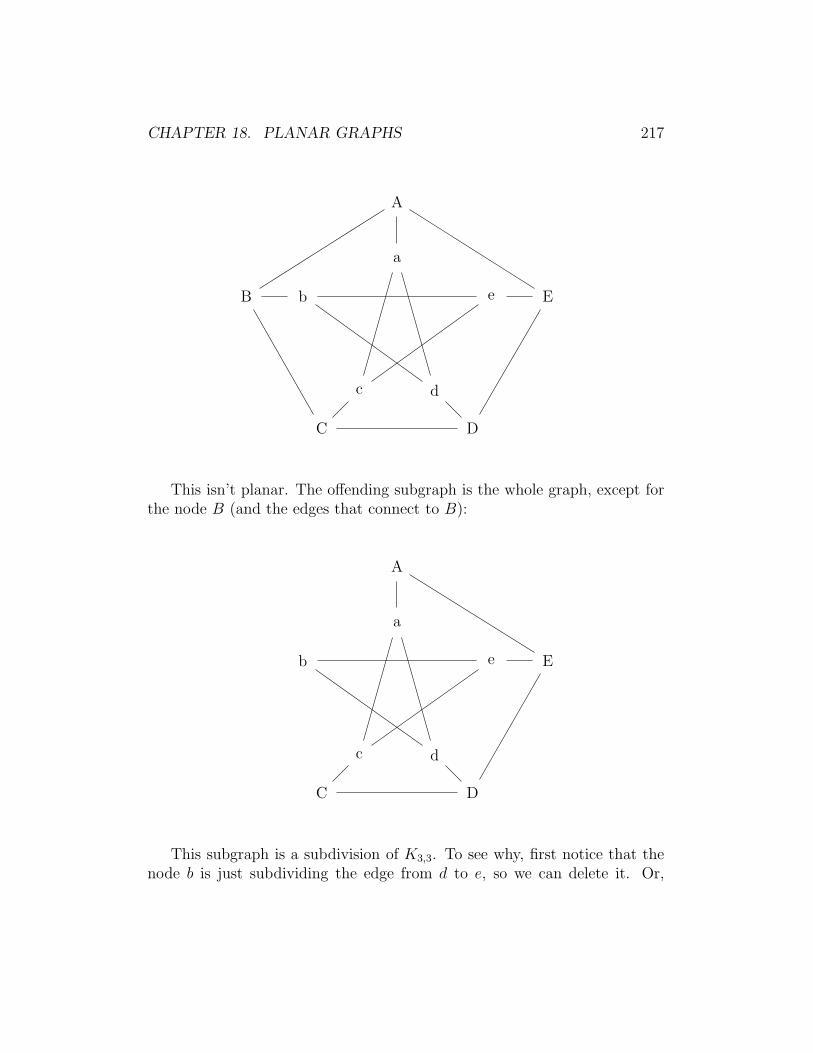
CHAPTER 18. PLANAR GRAPHS 217
A
B E
C D
a
b e
c d
This isn’t planar. The offending subgraph is the whole graph, except forthe node B (and the edges that connect to B):
A
E
C D
a
b e
c d
This subgraph is a subdivision of K3,3. To see why, first notice that thenode b is just subdividing the edge from d to e, so we can delete it. Or,

CHAPTER 18. PLANAR GRAPHS 218
formally, the previous graph is a subdivision of this graph:
A
E
C D
a
e
c d
In the same way, we can remove the nodes A and C, to eliminate unnec-essary subdivisions:
E
D
a
e
c d
Now deform the picture a bit and we see that we have K3,3.
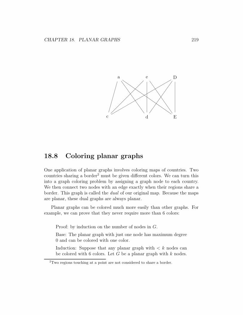
CHAPTER 18. PLANAR GRAPHS 219
E
Da e
c d
18.8 Coloring planar graphs
One application of planar graphs involves coloring maps of countries. Twocountries sharing a border2 must be given different colors. We can turn thisinto a graph coloring problem by assigning a graph node to each country.We then connect two nodes with an edge exactly when their regions share aborder. This graph is called the dual of our original map. Because the mapsare planar, these dual graphs are always planar.
Planar graphs can be colored much more easily than other graphs. Forexample, we can prove that they never require more than 6 colors:
Proof: by induction on the number of nodes in G.
Base: The planar graph with just one node has maximum degree0 and can be colored with one color.
Induction: Suppose that any planar graph with < k nodes canbe colored with 6 colors. Let G be a planar graph with k nodes.
2Two regions touching at a point are not considered to share a border.
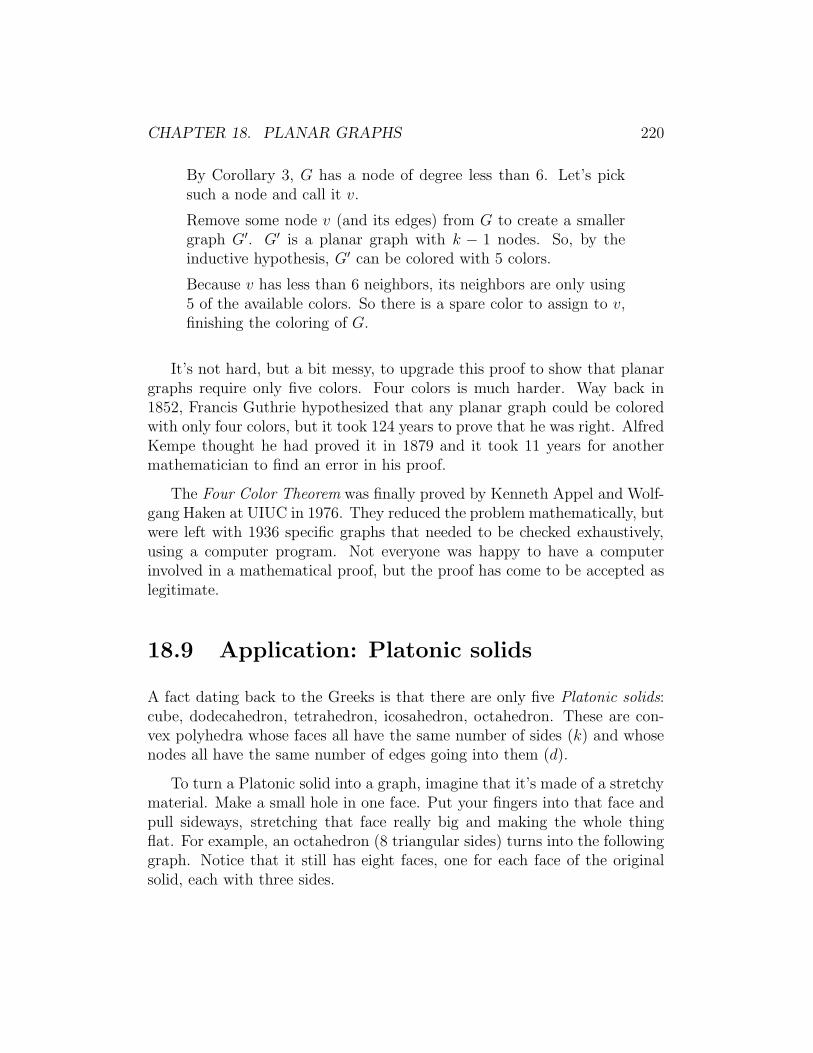
CHAPTER 18. PLANAR GRAPHS 220
By Corollary 3, G has a node of degree less than 6. Let’s picksuch a node and call it v.
Remove some node v (and its edges) from G to create a smallergraph G′. G′ is a planar graph with k − 1 nodes. So, by theinductive hypothesis, G′ can be colored with 5 colors.
Because v has less than 6 neighbors, its neighbors are only using5 of the available colors. So there is a spare color to assign to v,finishing the coloring of G.
It’s not hard, but a bit messy, to upgrade this proof to show that planargraphs require only five colors. Four colors is much harder. Way back in1852, Francis Guthrie hypothesized that any planar graph could be coloredwith only four colors, but it took 124 years to prove that he was right. AlfredKempe thought he had proved it in 1879 and it took 11 years for anothermathematician to find an error in his proof.
The Four Color Theorem was finally proved by Kenneth Appel and Wolf-gang Haken at UIUC in 1976. They reduced the problem mathematically, butwere left with 1936 specific graphs that needed to be checked exhaustively,using a computer program. Not everyone was happy to have a computerinvolved in a mathematical proof, but the proof has come to be accepted aslegitimate.
18.9 Application: Platonic solids
A fact dating back to the Greeks is that there are only five Platonic solids:cube, dodecahedron, tetrahedron, icosahedron, octahedron. These are con-vex polyhedra whose faces all have the same number of sides (k) and whosenodes all have the same number of edges going into them (d).
To turn a Platonic solid into a graph, imagine that it’s made of a stretchymaterial. Make a small hole in one face. Put your fingers into that face andpull sideways, stretching that face really big and making the whole thingflat. For example, an octahedron (8 triangular sides) turns into the followinggraph. Notice that it still has eight faces, one for each face of the originalsolid, each with three sides.
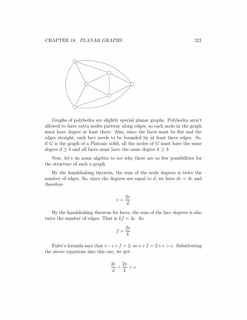
CHAPTER 18. PLANAR GRAPHS 221
Graphs of polyhedra are slightly special planar graphs. Polyhedra aren’tallowed to have extra nodes partway along edges, so each node in the graphmust have degree at least three. Also, since the faces must be flat and theedges straight, each face needs to be bounded by at least three edges. So,if G is the graph of a Platonic solid, all the nodes of G must have the samedegree d ≥ 3 and all faces must have the same degree k ≥ 3.
Now, let’s do some algebra to see why there are so few possibilities forthe structure of such a graph.
By the handshaking theorem, the sum of the node degrees is twice thenumber of edges. So, since the degrees are equal to d, we have dv = 2e andtherefore
v =2e
d
By the handshaking theorem for faces, the sum of the face degrees is alsotwice the number of edges. That is kf = 2e. So
f =2e
k
Euler’s formula says that v−e+f = 2, so v+f = 2+e > e. Substitutingthe above equations into this one, we get:
2e
d+
2e
k> e

CHAPTER 18. PLANAR GRAPHS 222
Dividing both sides by 2e:
1
d+
1
k>
1
2
If we analyze this equation, we discover that d and k can’t both be largerthan 3. If they were both 4 or above, the left side of the equation would be≤ 1
2. Since we know that d and k are both ≥ 3, this implies that one of the
two is actually equal to three and the other is some integer that is at least 3.
Suppose we set d to be 3. Then the equation becomes 13+ 1
k> 1
2. So
1k> 1
6, which means that k can’t be any larger than 5. Similarly, if k is 3,
then d can’t be any larger than 5.
This leaves us only five possibilities for the degrees d and k: (3, 3), (3, 4),(3, 5), (4, 3), and (5, 3). Each of these corresponds to one of the Platonicsolids.

Appendix A
Jargon
Mathematicians write in a dialect of English that differs from everyday En-glish and from formal scientific English. To read and write mathematicsfluently, you need to be aware of the differences.
A.1 Strange technical terms
Many technical terms, abbreviations, and shorthand symbols are easy totrack down. Perhaps they belong to an obvious topic area. Perhaps theyare used so heavily that no one forgets what they mean. Perhaps they areeasily found on Wikipedia. But others seem to appear mysteriously out ofnowhere.
abuse of notation The author is using a notation that doesn’t technicallycomply with the rules of mathematical writing, but is very convenient orconventional. For example, using “if” in a a definition where we reallymean “if and only if.” Or writing f(2, 3) for the result of applying fto the pair (2, 3). Strictly we should have written f((2, 3)), but no oneexcept a computer program would ever do that.
∃! This is the unique existence quantifier. ∃!x, P (x) means that there isexactly one x for which P (x) holds.
By symmetry A variant wording for “without loss of generality.”
223

APPENDIX A. JARGON 224
IH Inductive hypothesis, as in a proof by induction.
QED Short for “quod erat demonstrandum.” This is just the Latin transla-tion of “which is what we needed to show.” The Latin and the Englishversions are both polite ways to tell your reader that the proof is fin-ished.
tuple A generalization of “pair,” “triple,” etc to larger numbers of items.A k-tuple is an ordered sequence of k items. One occasionally hears“2-tuple” in place of “pair.”
NTS Need to show, as in “we need to show that all horses have four legs.”
WLOG, WOLOG, without loss of generality We’re stipulating an ex-tra fact or relationship, but claiming that it doesn’t actually add anynew information to the problem. For example, if we have two real vari-ables x and y, with identical properties so far, it’s ok to stipulate thatx ≤ y because we’re simply fixing which of the two names refers to thesmaller number.
A.2 Odd uses of normal words
In addition to the obvious technical terms (e.g. “rational number”), somewords are used rather differently in mathematics than in everyday English.
Clearly See “obviously.”
Consider The author is about to pull an example or constant or the like outof thin air. Typically, this part of the proof was constructed backwards,and the reasons for this step will not become apparent until later inthe proof.
Distinct Not equal. For example, if x and y are chosen to be “distinctelements” of a set A, then x and y aren’t allowed to have the samevalue.
Graph Might be a picture showing the relationship between two variables,or it might be a diagram with nodes and links between them.
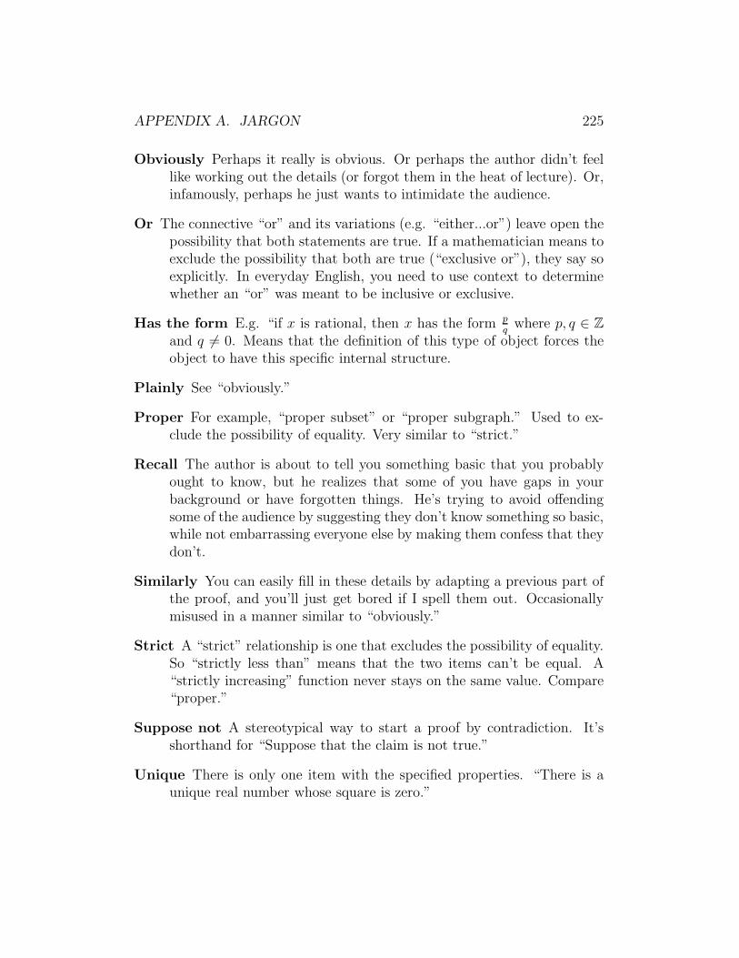
APPENDIX A. JARGON 225
Obviously Perhaps it really is obvious. Or perhaps the author didn’t feellike working out the details (or forgot them in the heat of lecture). Or,infamously, perhaps he just wants to intimidate the audience.
Or The connective “or” and its variations (e.g. “either...or”) leave open thepossibility that both statements are true. If a mathematician means toexclude the possibility that both are true (“exclusive or”), they say soexplicitly. In everyday English, you need to use context to determinewhether an “or” was meant to be inclusive or exclusive.
Has the form E.g. “if x is rational, then x has the form p
qwhere p, q ∈ Z
and q 6= 0. Means that the definition of this type of object forces theobject to have this specific internal structure.
Plainly See “obviously.”
Proper For example, “proper subset” or “proper subgraph.” Used to ex-clude the possibility of equality. Very similar to “strict.”
Recall The author is about to tell you something basic that you probablyought to know, but he realizes that some of you have gaps in yourbackground or have forgotten things. He’s trying to avoid offendingsome of the audience by suggesting they don’t know something so basic,while not embarrassing everyone else by making them confess that theydon’t.
Similarly You can easily fill in these details by adapting a previous part ofthe proof, and you’ll just get bored if I spell them out. Occasionallymisused in a manner similar to “obviously.”
Strict A “strict” relationship is one that excludes the possibility of equality.So “strictly less than” means that the two items can’t be equal. A“strictly increasing” function never stays on the same value. Compare“proper.”
Suppose not A stereotypical way to start a proof by contradiction. It’sshorthand for “Suppose that the claim is not true.”
Unique There is only one item with the specified properties. “There is aunique real number whose square is zero.”
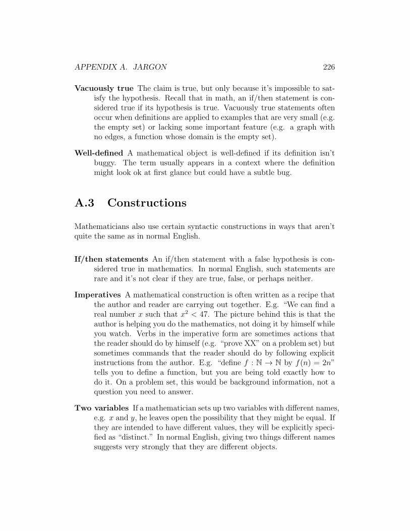
APPENDIX A. JARGON 226
Vacuously true The claim is true, but only because it’s impossible to sat-isfy the hypothesis. Recall that in math, an if/then statement is con-sidered true if its hypothesis is true. Vacuously true statements oftenoccur when definitions are applied to examples that are very small (e.g.the empty set) or lacking some important feature (e.g. a graph withno edges, a function whose domain is the empty set).
Well-defined A mathematical object is well-defined if its definition isn’tbuggy. The term usually appears in a context where the definitionmight look ok at first glance but could have a subtle bug.
A.3 Constructions
Mathematicians also use certain syntactic constructions in ways that aren’tquite the same as in normal English.
If/then statements An if/then statement with a false hypothesis is con-sidered true in mathematics. In normal English, such statements arerare and it’s not clear if they are true, false, or perhaps neither.
Imperatives A mathematical construction is often written as a recipe thatthe author and reader are carrying out together. E.g. “We can find areal number x such that x2 < 47. The picture behind this is that theauthor is helping you do the mathematics, not doing it by himself whileyou watch. Verbs in the imperative form are sometimes actions thatthe reader should do by himself (e.g. “prove XX” on a problem set) butsometimes commands that the reader should do by following explicitinstructions from the author. E.g. “define f : N → N by f(n) = 2n”tells you to define a function, but you are being told exactly how todo it. On a problem set, this would be background information, not aquestion you need to answer.
Two variables If a mathematician sets up two variables with different names,e.g. x and y, he leaves open the possibility that they might be equal. Ifthey are intended to have different values, they will be explicitly speci-fied as “distinct.” In normal English, giving two things different namessuggests very strongly that they are different objects.
APPENDIX A. JARGON 227
No resetting Do not change the value of a variable in the middle of a proof.Instead, use a fresh variable name. For example, suppose you know thatp = 3jk + 1 in a proof about divisibility. To simplify the form of theequation, it’s tempting to reset j to be three times its original value,so that you have p = jk+1. This isn’t done in standard mathematicalwriting. Instead, use a fresh variable name, e.g. s = 3j and thenp = sk + 1.
Variable names can be re-used when the context changes (e.g. you’vestarted a new proof). When working through a series of examples, e.g.a bunch of example functions to be discussed, rotate variable names, sothat the new definition appears after the reader has had time to forgetthe old definition.
Variable names Variable names are single-letter, e.g. f but not foo. Theletter can be adorned with a wide variety of accents, subscripts, andsuperscripts, however.
A.4 Unexpectedly normal
Mathematicians are, of course, underlyingly speakers of normal English. So,sometimes, they apply the normal rules of conversational English even whenthese aren’t part of the formal mathematical system.
names of variables In principle, any letter can be used as the name for anyvariable you need in a proof, with or without accent marks of varioussorts. However, there are strong conventions favoring certain names.E.g. x is a real number, n is an integer, f is a function, and T is a set.Observe what names authors use in your specific topic area and don’tstray too far from their conventions.
topics of equations Proofs are conversations about particular objects (e.g.polynomials, summations). Therefore, equations and other statementsare often about some specific topic object, whose properties are beingdescribed. When this is the case, the topic belongs on the lefthandside, just like the subject of a normal sentence.
Appendix B
Acknowledgements andSupplementary Readings
Most of the basic ideas and examples in this book date back many years andtheir original source is almost impossible to trace. I’ve consulted so manybooks and worked with so many helpful teachers, students, and course staffover the years that the details have blended into a blur. Nevertheless, certainbooks have had a particularly strong influence on my presentation. Most ofthem would make excellent supplementary materials, both for instructorsand for students.
It’s impossible to even think about discrete mathematics without citingthe classic encyclopedic text by Rosen [Rosen 2007]. It helped me under-stand what topics would be most relevant to a computer science, as op-posed to a mathematics, audience. Biggs [Biggs 2002], Matousek and Nesetril[Matousek and Nesetril 1998] and West [West 2001] have been invaluable ref-erences for discrete mathematics and graph theory.
From Liebeck [Liebeck 2006], Sipser [Sipser 2006], and Biggs [Biggs 2002],I learned how to extract core concepts and present them concisely. FromFendel and Resek [Fendel and Resek 1990], I learned how to explain proofmechanics and talk about the process of constructing proofs. From my nu-merous students and course staff, both at Iowa and Illinois, I have learnedto understand why some of these concepts seem so hard to beginners. Myco-instructors Eric Shaffer and Viraj Kumar helped mould the curriculum to
228

APPENDIX B. ACKNOWLEDGEMENTS AND SUPPLEMENTARY READINGS229
the needs of our students. Sariel Har-Peled has provided many interestingexamples.
Finally, a special individual citation goes to Jeff Erickson for the recur-sion fairy (though my fairy has a slightly different job than his) and forextended arguments about the proper way to present induction (though westill disagree).
Bibliography
[Biggs 2002] Norman L. Biggs (2002) Discrete Mathematics, second edition,Oxford University Press, Oxford, UK.
[Fendel and Resek 1990] Daniel Fendel and Diane Resek (1990) Foundationsof Higher Mathematics: Exploration and Proof, Addison-Wesley, ReadingMA.
[Liebeck 2006] Martin Liebeck (2006) A Concise Introduction to Pure Math-ematics, Chapman Hall/CRC, Boca Raton, FL.
[Matousek and Nesetril 1998] Jiri Matousek and Jaroslav Nesetril (1998) In-vitation to Discrete Mathematics Oxford University Press.
[Rosen 2007] Kenneth H. Rosen (2007) Discrete Mathematics and Its Appli-cations, sixth edition, McGraw Hill, New York, NY.
[Sipser 2006] Michael Sipser, Introduction to the Theory of Computation, sec-ond edition, Thomson, Boston MA.
[West 2001] Douglas B. West (2001) Introduction to Graph Theory, secondedition, Prentice-Hall, Upper Saddle River, NJ.
230