bujagali ii – economic and financial evaluation...
TRANSCRIPT
Bujagali II – Economic and Financial Evaluation Study
Final Report
Main Text
February 2007
International Finance Corporation Bujagali II: Economic and Financial Evaluation Study Final Report 2 February 2007 26/02/2007-20224
LIST OF ABBREVIATIONS USED IN THE REPORT......................................................................5 EXECUTIVE SUMMARY .......................................................................................................................8 1 INTRODUCTION..........................................................................................................................18
1.1 BACKGROUND .........................................................................................................................18 1.2 OBJECTIVES AND SCOPE OF WORK .........................................................................................19
2 ELECTRICITY DEMAND FORECAST ...................................................................................20 2.1 INTRODUCTION........................................................................................................................20 2.2 PRESENT AND PAST DEMAND .................................................................................................20 2.3 METHODOLOGY AND ASSUMPTIONS.......................................................................................27 2.4 PROJECTIONS FOR UGANDAN ECONOMY ................................................................................27
2.4.1 General ..............................................................................................................................27 2.4.2 Overview of the Ugandan Economy..................................................................................27 2.4.3 Projections.........................................................................................................................28
2.5 ASSUMPTIONS FOR RESIDENTIAL SECTOR..............................................................................28 2.6 ASSUMPTIONS FOR COMMERCIAL AND INDUSTRIAL SECTORS...............................................31 2.7 REVENUE COLLECTION ...........................................................................................................31 2.8 TARIFF ASSUMPTIONS.............................................................................................................32 2.9 ASSUMPTIONS ON REDUCTION OF SYSTEM LOSSES................................................................33 2.10 ELECTRICITY EXPORTS ...........................................................................................................35 2.11 LOAD FORECAST RESULTS AND SENSITIVITY SCENARIOS .....................................................36
3 HYDROLOGY AND ENERGY GENERATION OF HYDRO POWER PLANTS..............41 3.1 INTRODUCTION........................................................................................................................41 3.2 LAKE VICTORIA NET BASIN SUPPLY ......................................................................................41 3.3 DEPARTURE FROM THE AGREED CURVE AND THE RECENT FALL IN THE LEVEL OF LAKE VICTORIA ...............................................................................................................................................46 3.4 LAKE OPERATION MODELLING AND ENERGY GENERATION EVALUATION ...........................47
4 INTERIM SUPPLY ARRANGEMENTS (2006-2010)..............................................................52 4.1 EXISTING SHORT TERM THERMAL PLANT..............................................................................52 4.2 ADDITIONAL EMERGENCY THERMAL PLANT .........................................................................52 4.3 BIOMASS PROJECTS.................................................................................................................52 4.4 SMALL HYDRO PROJECTS .......................................................................................................53 4.5 FUEL SUPPLY ISSUES...............................................................................................................54 4.6 FUEL TYPES AND COSTS .........................................................................................................55 4.7 INTERIM GENERATING PLANT.................................................................................................58 4.8 ELECTRICITY IMPORTS............................................................................................................59 4.9 PLANT EXISTING IN 2011 ........................................................................................................59
5 CANDIDATE PLANT (2011-2020) .............................................................................................61 5.1 CONVENTIONAL THERMAL PLANT..........................................................................................61 5.2 GEOTHERMAL POTENTIAL IN UGANDA...................................................................................64 5.3 EXISTING HYDRO ....................................................................................................................66 5.4 BUJAGALI HPP........................................................................................................................68
5.4.1 Characteristics of the project............................................................................................68 5.4.2 Construction Costs ............................................................................................................70 5.4.3 Other costs and resulting total cost of implementation....................................................71 5.4.4 Range of capital costs variations for risk analysis...........................................................74
5.5 KARUMA HPP .........................................................................................................................75 5.5.1 Characteristics of the project............................................................................................75 5.5.2 Construction costs .............................................................................................................76

International Finance Corporation Bujagali II: Economic and Financial Evaluation Study Final Report 3 February 2007 26/02/2007-20224
5.5.3 Other costs and resulting total cost of implementation....................................................77 5.6 OTHER CANDIDATE HYDRO....................................................................................................79
5.6.1 Other major hydro power projects....................................................................................79 5.6.2 Small and Medium Scale Hydro........................................................................................79
6 ENVIRONMENTAL AND SOCIAL COSTS ............................................................................81 6.1 INTRODUCTION........................................................................................................................81 6.2 ENVIRONMENTAL COSTS AND BENEFITS OF BUJAGALI..........................................................81
6.2.1 Dam and Power Station ....................................................................................................81 6.2.2 Transmission Line .............................................................................................................82 6.2.3 Environmental Benefits .....................................................................................................83
6.3 SOCIAL COSTS AND BENEFITS OF BUJAGALI ..........................................................................84 6.3.1 Compensation and Resettlement of Dam and Power House............................................84 6.3.2 Community Development Action Plan – CDAP ...............................................................85 6.3.3 Transmission Line .............................................................................................................86 6.3.4 Social costs by year ...........................................................................................................87
6.4 ENVIRONMENTAL COSTS AND BENEFITS OF KARUMA ...........................................................88 6.4.1 Introduction .......................................................................................................................88 6.4.2 Environmental Impacts......................................................................................................89 6.4.3 Social Impacts....................................................................................................................89 6.4.4 Mitigation and Compensation Measures ..........................................................................91 6.4.5 Environmental and Social Costs .......................................................................................92 6.4.6 E&S costs by year..............................................................................................................94 6.4.7 Environmental Benefits .....................................................................................................95
7 LEAST COST EXPANSION PLAN............................................................................................97 7.1 OBJECTIVES.............................................................................................................................97 7.2 PLANNING CRITERIA, METHODOLOGY AND BASIC DATA ......................................................97
7.2.1 Computer tool and methodology.......................................................................................97 7.2.2 Planning Period.................................................................................................................98 7.2.3 Demand forecast................................................................................................................98 7.2.4 Reliability Criteria...........................................................................................................100 7.2.5 Economic Criteria ...........................................................................................................101 7.2.6 Characteristics of Thermal Plants ..................................................................................101 7.2.7 Characteristics of Hydro Power Plants..........................................................................104
7.3 POWER GENERATION SITUATION IN 2011 ............................................................................106 7.4 ANALYSIS OF LEAST COST EXPANSION PLANS ....................................................................107
7.4.1 Presentation of the cases considered ..............................................................................107 7.4.2 Main Results and Conclusions of the Analysis ...............................................................108 7.4.3 Analysis of Least-Cost Expansion Plans for the Reference Cases.................................112 7.4.4 Analysis of Least-Cost Expansion Plans for sensitivity cases........................................117
7.5 RISK ANALYSIS .....................................................................................................................120 8 ECONOMIC RATE OF RETURN............................................................................................125
8.1 METHODOLOGY ....................................................................................................................125 8.2 ASSUMPTIONS .......................................................................................................................125
8.2.1 Baseline Assumptions for Incremental Costs and Demand............................................125 8.2.2 System Expansion Costs ..................................................................................................126 8.2.3 Reduction in Greenhouse Gas Emissions .......................................................................126 8.2.4 Incremental Demand .......................................................................................................127 8.2.5 Residual Displaced Thermal Energy ..............................................................................128 8.2.6 Unserved Energy Cost.....................................................................................................128
8.3 BENEFIT ASSUMPTIONS.........................................................................................................129 8.3.1 Household Willingness-to-Pay........................................................................................129 8.3.2 Industrial and Commercial Willingness-to-Pay .............................................................129 8.3.3 Export Willingness-to-Pay ..............................................................................................129
International Finance Corporation Bujagali II: Economic and Financial Evaluation Study Final Report 4 February 2007 26/02/2007-20224
8.4 EXPECTED EIRR ...................................................................................................................130 8.4.1 General ............................................................................................................................130 8.4.2 High Hydrology ...............................................................................................................130 8.4.3 Low Hydrology ................................................................................................................130
8.5 SENSITIVITY STUDIES AND RISK ANALYSIS .........................................................................135 8.5.1 General ............................................................................................................................135 8.5.2 Sensitivity to Demand Scenario ......................................................................................135 8.5.3 Sensitivity to Fuel Price Scenario ...................................................................................135 8.5.4 Sensitivity to Bujagali Capital Cost Scenario.................................................................136
8.6 RISK ANALYSIS .....................................................................................................................136 8.7 CONCLUSIONS .......................................................................................................................138
9 FINANCIAL FEASIBILITY......................................................................................................140 9.1 OBJECTIVES AND OUTPUTS ...................................................................................................140 9.2 REVIEW OF TARIFF METHODOLOGY ......................................................................................140
9.2.1 Tariff methodology for existing licensed generators......................................................141 9.2.2 Tariff methodology for other licensed generators ..........................................................141 9.2.3 Tariff methodology for planned and future generators ..................................................142 9.2.4 Tariff methodology for UETCL.......................................................................................142 9.2.5 Tariff methodology for Umeme .......................................................................................143 9.2.6 Subsidies ..........................................................................................................................145 9.2.7 Tariff stabilisation ...........................................................................................................146
9.3 REVIEW OF TARIFF MODELS AND MODEL DEVELOPMENT .....................................................146 9.4 COLLECTION OF DATA...........................................................................................................148
9.4.1 Inflation and exchange rates ...........................................................................................148 9.4.2 Demand forecast and losses............................................................................................149 9.4.3 Generation costs ..............................................................................................................150 9.4.4 Transmission costs...........................................................................................................153 9.4.5 Distribution costs.............................................................................................................155 9.4.6 Regulatory parameters ....................................................................................................156
9.5 RESULTS................................................................................................................................158 9.5.1 Revenue requirements in the electricity sector ...............................................................158 9.5.2 Comparing costs of supply with assumed tariffs ............................................................158 9.4.7 Impact of lower tariffs on demand forecast ....................................................................160
10 MACRO-ECONOMIC ANALYSIS ..........................................................................................162 10.1 SUMMARY .............................................................................................................................162 10.2 MACRO-ECONOMIC PARAMETERS ........................................................................................163
10.2.1 Availability of Modelling Tools..................................................................................163 10.2.2 Developments up to 2011 – the starting point ...........................................................163
10.3 EFFECTS ON GDP COMPONENTS...........................................................................................163 10.3.1 Household consumption .............................................................................................163 10.3.2 General government consumption and investment....................................................164 10.3.3 Business investment ....................................................................................................164 10.3.4 Exports ........................................................................................................................166 10.3.5 Imports ........................................................................................................................166 10.3.6 Impacts on Balance of Payments and the Exchange Rate.........................................167
10.4 EFFECTS ON THE GOVERNMENT’S FINANCIAL POSITION ......................................................171
International Finance Corporation Bujagali II: Economic and Financial Evaluation Study Final Report 5 February 2007 26/02/2007-20224
List of Abbreviations used in the Report
ADO Automotive Diesel Oil
AGO Automotive Gas Oil
BEL Bujagali Electricity Limited
BIU Bujagali Implementation Unit
BOT Build, Operate and Transfer
BoU Bank of Uganda
C&R Compensation and Resettlement
CCGT Combined Cycle Gas Turbine
CDAP Community Development Action Plan
cSt Centi-Stokes
CUE Cost of Unserved Energy
DWD Department for Water Development
E&S Environmental and Social
EPC Engineer procurement and construct
ERA Electricity Regulatory Authority
ESIA Environmental and Social Impact Assessment
ESMAP Energy Strategy & Management Action Program
EV Evaporation
FOB Free on board
GDP Gross Domestic Product
GHG Greenhouse Gases
GoU Government of Uganda
GT Gas Turbine
HFO Heavy Fuel Oil
HPP Hydro Power Plant
HV High Voltage
IAEA International Atomic Energy Authority
IDA International Development Agency
IDC Interest during construction
IDO Industrial Diesel Oil
IMF International Monetary Fund

International Finance Corporation Bujagali II: Economic and Financial Evaluation Study Final Report 6 February 2007 26/02/2007-20224
IPP Independent Power Producer
ISO International Standards Organisation
KPLC Kenya Power & Lighting Company Limited
LDC Load Duration Curve
LOLP Loss of Load Probability
LSD Low Speed Diesel
LHV Lower heating value
Masl Metres above sea level
MoFPED Ministry of Finance Planning and Economic Development
MSD Medium Speed Diesel
MW Megawatt
NBS Net Basin Supply
NGO Non-Governmental Organisation
NPV Net Present Value
PPA Power Purchase Agreement
PW Present-worth
RAP Resettlement Action Plan
RE Rural Electrification
REA Rural Electrification Agency
RF Rainfall
RO Runoff
ROW Right of way
SCADA Supervisory Control and Data Acquisition
SCOUL Sugar Company of Uganda Limited
STD Sexually-Transmitted Disease
ToR Terms of Reference
UBOS Uganda Bureau of Statistics
UEB Uganda Electricity Board
UEDCL Uganda Electricity Distribution Company Limited
UETCL Uganda Electricity Transmission Company Limited
US$ United States Dollar
US¢ United States cents

International Finance Corporation Bujagali II: Economic and Financial Evaluation Study Final Report 7 February 2007 26/02/2007-20224
USh Uganda Shilling
WASP Wien Automatic System Planning Package
WREM Water Resources and Environmental Management
WTI West Texas Intermediate
WTP Willingness-to-Pay
International Finance Corporation Bujagali II: Economic and Financial Evaluation Study Final Report 8 February 2007 26/02/2007-20224
Executive Summary
Power Planning Associates was appointed by the IFC in January 2006 to carry out an economic and financial evaluation study of the 250 MW Bujagali II hydropower project in Uganda. The ToR for the assignment are reproduced in Appendix A. The purpose of this study is to evaluate the economic viability of the Bujagali II project taking into account economic, financial, social and environmental aspects.
An Interim Report was submitted in February 2006; the report was presented to the Government of Uganda (GoU) and other stakeholders in Kampala in March 2006. Work was then held up for a number of months whilst the World Bank carried out an independent review of the analysis of the hydrology presented in the Interim Report. The demand forecast was also reviewed and amended to include updated GDP estimates and a detailed assessment of the assumptions of future levels of technical and commercial losses. The revised forecast was presented to GoU and other stakeholders in Kampala in September 2006.
The Draft Final Report was submitted to IFC in December 2006 and presented to the government and other stakeholders in Kampala in mid-January 2007. The report was also presented to the Bujagali lenders in London at the end of January.
We now present a brief synopsis of the results and conclusions of the study following the order of the sections in the Main Text of the Report. The Main Text volume is supported by Appendices which are included in a separate volume.
Background
The economic and financial analysis of the Bujagali project in this study includes an update for the hydrology of the lake and development of potential future hydrological scenarios, both for the short and medium term. Had the Bujagali project been commissioned in 2005/06, as envisaged back in 2000, the current problems would not have arisen, or at least not to the same extent. In the intervening years there has been continuing demand growth, coupled with severe supply constraints that would have been alleviated had Bujagali come into service in 2005. The experience has demonstrated the high cost penalties of long term delays in the Bujagali project that was needed to meet the growing electricity demand of Uganda.

International Finance Corporation Bujagali II: Economic and Financial Evaluation Study Final Report 9 February 2007 26/02/2007-20224
Electricity Demand Forecast for the Uganda System
A demand forecast for the Ugandan grid has been derived using the most recent data on the economy and the electricity sub-sector1. The forecast is predicated on assumptions for the growth of the economy, connection of new consumers, and the reduction of system losses, in particular commercial losses. The base case forecast is summarised in the table below.
Year Peak Demand
(MW) Generation (GWh net)
Sales (GWh)
2005 (actual) 354 1921 1131
2010 375 2208 1521
2015 545 2959 2361
2020 789 4287 3421 Note: Figures in table above exclude exports to Tanzania and Rwanda.
High and low sensitivity forecasts have also been derived based on alternative economic growth and consumer connection assumptions. The base, high and low forecasts are predicated on forecast tariffs during the period up to 2011 when Bujagali is expected to come into service. The tariff projections are based on the financial requirements of the short-term emergency thermal power generation programme and the estimated generation availability from Nalubaale – Kiira.
The 2007 to 2011 tariff assumptions have been derived from the detailed financial analysis of an independent consultant contracted by the World Bank as part of the appraisal of the emergency thermal power project, for which GoU is seeking IDA funding. The tariff assumptions are for increases in real tariffs of 37% in 2006, 45% in 20072 and 15% in 2008. A reduction of 15% is assumed in 2011, when the commissioning of Bujagali should reduce thermal generation substantially. The demand forecast, least cost planning studies and associated financial/tariff analysis were carried out on the basis of the above tariff assumptions. The resulting cost of supply and imputed tariffs were then checked against the original tariff assumptions to ensure that the price
1 Note: data collection for the demand forecast was carried out in January 2006.
2 Tariffs were in fact increased by approximately 42% in November 2006, which was not known when the load forecast was finalized. This increase will have its full impact on 2007 demand, almost in line with the Consultant’s assumption.
International Finance Corporation Bujagali II: Economic and Financial Evaluation Study Final Report 10 February 2007 26/02/2007-20224
elasticity effect which has been factored into the demand forecast remained valid. It was found that the assumed tariffs were above the cost of supply, post-2011, by approximately 1.2 US¢/kWh (7%). Even if the tariff were to drop in line with cost of supply, the positive impact on the demand forecast would be minimal.
Hydrology and Energy Outputs of Hydro Plants
A detailed review has been carried out of the hydrology of Lake Victoria. Our conclusion is that the whole period of record from 1900 should be used to determine the future dependable flow for power generation at hydro power stations on the Victoria Nile.
Significantly contrasting values of Net Basin Inflows (NBI) have been observed between the periods 1900 to 1960 and 1961 to 2000, and the low inflow situation observed since 1999. The approach to hydrological risk has been to adopt two separate hydrological flow release scenarios for the 20 year period after 2010 over which the evaluation is being conducted, corresponding to a low hydrology scenario and a high hydrology scenario. The high hydrology scenario is based on the period 1961 to 2000 and the low hydrology scenario on the period 1900 to 1960. The likelihood of the low hydrology occurring has been assessed substantially higher than the high hydrology. The relative probabilities have been calculated at 79%/21% for the low/high hydrology scenarios.
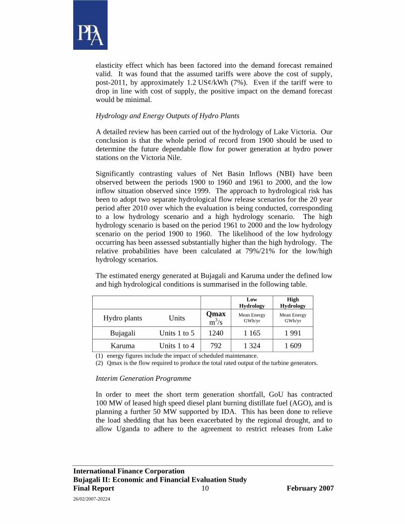
The estimated energy generated at Bujagali and Karuma under the defined low and high hydrological conditions is summarised in the following table.
Low Hydrology
High Hydrology
Hydro plants Units Qmax m3/s
Mean Energy GWh/yr
Mean Energy GWh/yr
Bujagali Units 1 to 5 1240 1 165 1 991
Karuma Units 1 to 4 792 1 324 1 609 (1) energy figures include the impact of scheduled maintenance. (2) Qmax is the flow required to produce the total rated output of the turbine generators.
Interim Generation Programme
In order to meet the short term generation shortfall, GoU has contracted 100 MW of leased high speed diesel plant burning distillate fuel (AGO), and is planning a further 50 MW supported by IDA. This has been done to relieve the load shedding that has been exacerbated by the regional drought, and to allow Uganda to adhere to the agreement to restrict releases from Lake
International Finance Corporation Bujagali II: Economic and Financial Evaluation Study Final Report 11 February 2007 26/02/2007-20224
Victoria to the “Agreed Curve”3. A further 50 MW of medium speed diesel plants burning heavy fuel oil (HFO) is expected to be installed as an Independent Power Project (IPP). The emergency thermal plant is intended to fill the generation capacity gap until 2011 when Bujagali is expected to enter service. The thermal plant will be supplemented by several small hydro projects to be developed as IPPs. In addition, UETCL has negotiated contracts with two sugar producers for 15 MW of power produced from bagasse (sugar cane residue).
Geothermal Potential
We have made a detailed review of the geothermal potential of Uganda and conclude that the resource may be substantially lower than previously estimated. It is considered that only approximately 40 MW of geothermal power generating capacity may be developed economically on the basis of present knowledge, as discussed in detail in Appendix D.
Bujagali and Karuma Cost Estimates
A detailed review and update of the cost estimates for Bujagali and Karuma has been carried out. These are considered to be the only two major hydro plant options for the medium term. These estimates take into consideration the information received from the Bujagali sponsor on the EPC contract negotiations and on development costs relating to Bujagali.
The total economic cost estimates for Bujagali and Karuma resulting from our review are as follows (in constant 2006 US$)4:
3 The “Agreed Curve” represents the allowable outflow from Lake Victoria into the Nile, corresponding to the flow that would have occurred in the absence of man-made intervention, e.g. the dam at Nalubaale-Kiira.
4 Just after this report was completed, BEL informed PPA and the Bank Group of the most recent results of on-going negotiations with the EPC contractor, indicating the addition of a $20 to $ 30 million risk premium in exchange for a comprehensive turnkey contract, plus another $ 5 to $10 million for improvements to the electro-mechanical works, bringing the total EPC cost increase into a range of $30 to $35 millions, nominal and undiscounted. At the same time, BEL and the contractor are negotiating an incentive scheme to accelerate commissioning by 3 to 4 months, which would create for Uganda a real economic cost saving on thermal plant operation estimated at $30 to $40 million (in dollars of 2006). The net impact of these proposed changes on the project’s economic viability is judged to be minimal.

International Finance Corporation Bujagali II: Economic and Financial Evaluation Study Final Report 12 February 2007 26/02/2007-20224
ITEM Bujagali 5 units (US$ million)
Karuma 4 units (US$ million)
Direct construction costs: - Civil works - Equipment
227 187
315 117
Connection to the grid 28 79
Engineering and coordination 28 33
Environmental and Social Impacts 26 15
Development Costs 25 29
Total Implementation Cost (excluding Interest During Construction) 521 588
Environmental and Social Costs of Bujagali and Karuma
The Consultant undertook a field mission to Uganda in July 2006 to collect data on the E&S costs of the Bujagali and Karuma projects. Moreover, Burnside, who prepared the Bujagali Social and Environmental Assessment reports, estimated the project’s environmental and social impact cost based on substantial and detailed field investigations and compilation of new cost data. We have reviewed and commented on the Burnside figures and have used them for the economic analysis of Bujagali. We have also prepared E&S cost estimates for Karuma based on the existing ESIA, which was undertaken in 1999. The cost estimates adopted for Karuma take cognisance of the higher unit cost rates derived from the Burnside studies. The total incremental E&S expenditures for Bujagali and Karuma are shown in the cost table above.
Least Cost Generation Expansion Plans
Detailed least cost generation expansion plans were developed for the Ugandan system for the period from 2010 to 2020 using the WASP IV system expansion program. The analysis was undertaken for base, high and low demand forecasts; low hydrology and high hydrology scenarios; base, low and high fuel price projections; and base, low and high Bujagali cost estimates. Alternative least cost sequences were determined for both the ‘with Bujagali’ and ‘without Bujagali’ cases. Karuma was retained as a candidate plant in both the ‘with Bujagali’ and ‘without Bujagali’ cases. A total of 72 cases were evaluated to cover the full risk analysis, and 13 further cases were considered for additional sensitivity analysis. The main results showed that Bujagali commissioned in 2011 was part of the least cost programme under all demand forecast scenarios with the low hydrology, and also for the high and base

International Finance Corporation Bujagali II: Economic and Financial Evaluation Study Final Report 13 February 2007 26/02/2007-20224
demand with high hydrology. In the high hydrology, low demand cases, the least cost expansion plan comprises only new thermal plant up to 2020, i.e. neither Bujagali nor Karuma could be justified. However, the total probability of occurrence of these cases is low, estimated at 5.5%, and the maximum probability of any one case occurring is only 1.5%.
Sensitivity studies were carried out to confirm the optimum timing of Bujagali, by delaying commissioning from 2011 to 2012 for the base demand. This leads to higher present worth (PW) costs for the low hydrology and marginally higher costs for the high hydrology. The analysis also showed that a 4-unit Bujagali design was less attractive economically than the 5-unit reference design. A further sensitivity study confirmed that Karuma commissioned before Bujagali (by forcing Karuma in 2012) leads to higher PW costs, and that the cost of Bujagali would need to increase by 49%5 to justify the commissioning of Karuma as the next plant before Bujagali.
A full risk analysis was made for the ‘with Bujagali’ and ‘without Bujagali’ cases, with the following probabilities assigned to the key variables:
Demand forecast: base/high/low - 40%/30%/30%
Hydrology: high/low - 21%/79%
Fuel Prices base/low/high – 40%/30%/30%
Bujagali Cost base/low/high - 60%/20%/20%
Assigning the probability weightings to the PW costs resulted in a total net present value (NPV) advantage of US$ 184.0 million (in 2006 US$ with discounting to 2006) in favour of the ‘with Bujagali’ cases. The NPV value is robust in respect of the assumption on hydrology. For example, if 100% probability is assigned to either the low or the high hydrology scenarios, the NPVs, representing the differences between the ‘with Bujagali’ and ‘without Bujagali’ programmes, are:
Low hydrology US$ 202 million, and
High hydrology US$ 116 million
in favour of the ‘with Bujagali’ cases.
Bujagali Economic Internal Rate of Return (EIRR)
5 This result was obtained by progressively increasing the cost of Bujagali in the simulation analysis until the WASP program no longer selected Bujagali as the next major plant. In this case the least cost sequence included Karuma in 2012.

International Finance Corporation Bujagali II: Economic and Financial Evaluation Study Final Report 14 February 2007 26/02/2007-20224
The EIRR for the Bujagali project was estimated by evaluating the cost and benefits of the project in terms of the capital and operating costs of Bujagali and the incremental transmission and distribution capital and operating costs associated with meeting the increment of demand supplied by the project. The benefits were measured in terms of the displacement of costly thermal power and incremental demand of the various categories of consumer, that is met by Bujagali, valued at their respective willingness to pay.
The EIRR values for the references cases obtained are summarised in the table below.
High hydrology Low Hydrology
EIRR 21.7% 22.0%
When the benefits of avoided greenhouses cases are included the EIRRs increase to 22.0% for the high hydrology and 22.9% for the low hydrology.
Sensitivity studies indicate that the project EIRR is robust against all key risk factors, including: hydrology, demand forecast, fuel prices and the capital cost of the project. The demand scenario has the greatest impact on EIRR, but in the most adverse combination of scenarios using the low demand case the resulting EIRR value of 12.5% remains comfortably greater than the 10% benchmark discount rate for World Bank Group-supported projects.
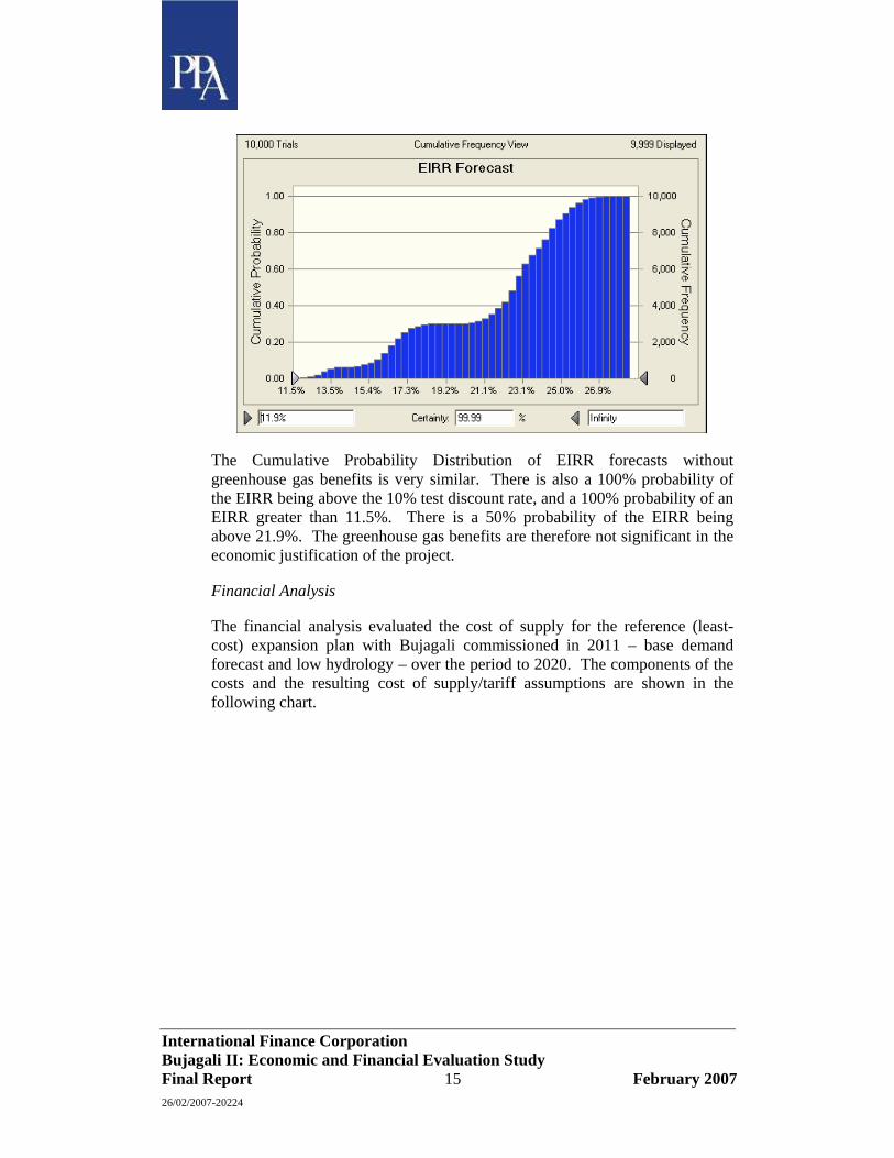
In addition to the sensitivity studies, a probabilistic risk analysis was undertaken on the EIRR value using the Crystal Ball software package with the following parameters subject to a probabilistic range of outcomes: demand forecast, crude oil price, Bujagali capital cost, T&D capital costs, willingness-to-pay of newly-connected customers, and hydrology. The following chart presents the Cumulative Probability Distribution of EIRR forecasts including the impact of greenhouse gas credits to the project. This chart shows there is a 100% probability of the EIRR being above the 10% benchmark discount rate, and a 100% probability of an EIRR greater than 11.7%. The same cumulative probability distribution can be used to show that there is a 50% probability of the EIRR being above 22.7%.
International Finance Corporation Bujagali II: Economic and Financial Evaluation Study Final Report 15 February 2007 26/02/2007-20224
The Cumulative Probability Distribution of EIRR forecasts without greenhouse gas benefits is very similar. There is also a 100% probability of the EIRR being above the 10% test discount rate, and a 100% probability of an EIRR greater than 11.5%. There is a 50% probability of the EIRR being above 21.9%. The greenhouse gas benefits are therefore not significant in the economic justification of the project.
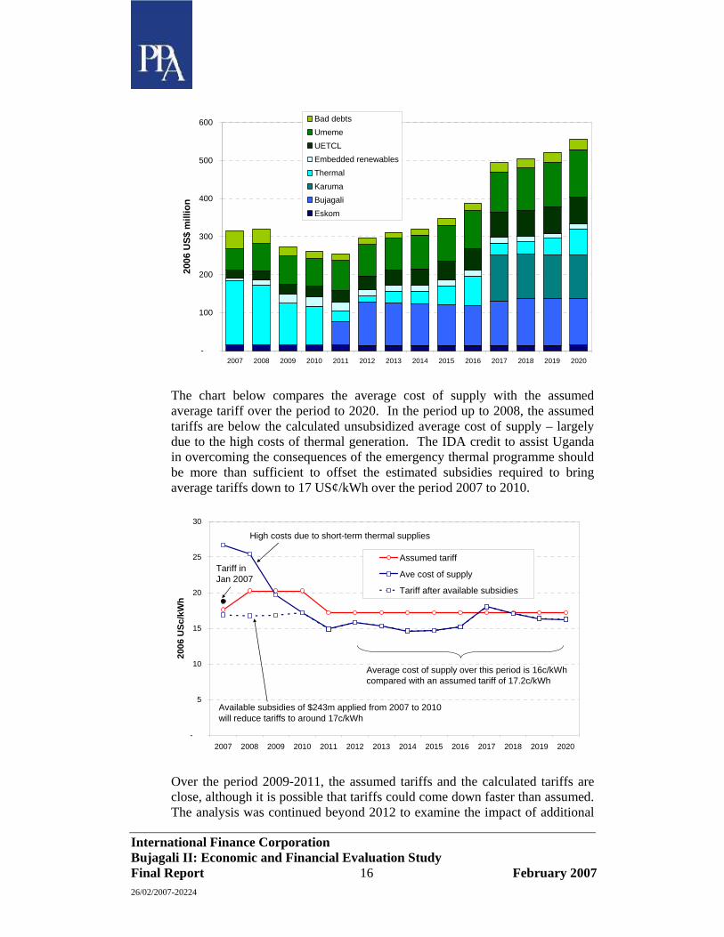
Financial Analysis
The financial analysis evaluated the cost of supply for the reference (least-cost) expansion plan with Bujagali commissioned in 2011 – base demand forecast and low hydrology – over the period to 2020. The components of the costs and the resulting cost of supply/tariff assumptions are shown in the following chart.
International Finance Corporation Bujagali II: Economic and Financial Evaluation Study Final Report 16 February 2007 26/02/2007-20224
-
100
200
300
400
500
600
2007 2008 2009 2010 2011 2012 2013 2014 2015 2016 2017 2018 2019 2020
2006
US$
mill
ion
Bad debtsUmemeUETCLEmbedded renewablesThermalKarumaBujagaliEskom
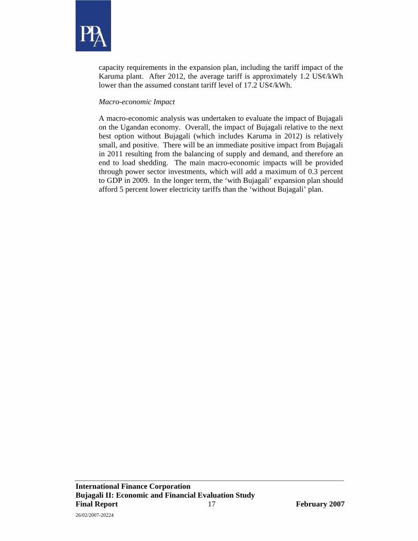
The chart below compares the average cost of supply with the assumed average tariff over the period to 2020. In the period up to 2008, the assumed tariffs are below the calculated unsubsidized average cost of supply – largely due to the high costs of thermal generation. The IDA credit to assist Uganda in overcoming the consequences of the emergency thermal programme should be more than sufficient to offset the estimated subsidies required to bring average tariffs down to 17 US¢/kWh over the period 2007 to 2010.
-
5
10
15
20
25
30
2007 2008 2009 2010 2011 2012 2013 2014 2015 2016 2017 2018 2019 2020
2006
USc
/kW
h
Assumed tariff
Ave cost of supply
Tariff after available subsidies
Tariff in Jan 2007
Average cost of supply over this period is 16c/kWhcompared with an assumed tariff of 17.2c/kWh
High costs due to short-term thermal supplies
Available subsidies of $243m applied from 2007 to 2010 will reduce tariffs to around 17c/kWh
Over the period 2009-2011, the assumed tariffs and the calculated tariffs are close, although it is possible that tariffs could come down faster than assumed. The analysis was continued beyond 2012 to examine the impact of additional
International Finance Corporation Bujagali II: Economic and Financial Evaluation Study Final Report 17 February 2007 26/02/2007-20224
capacity requirements in the expansion plan, including the tariff impact of the Karuma plant. After 2012, the average tariff is approximately 1.2 US¢/kWh lower than the assumed constant tariff level of 17.2 US¢/kWh.
Macro-economic Impact
A macro-economic analysis was undertaken to evaluate the impact of Bujagali on the Ugandan economy. Overall, the impact of Bujagali relative to the next best option without Bujagali (which includes Karuma in 2012) is relatively small, and positive. There will be an immediate positive impact from Bujagali in 2011 resulting from the balancing of supply and demand, and therefore an end to load shedding. The main macro-economic impacts will be provided through power sector investments, which will add a maximum of 0.3 percent to GDP in 2009. In the longer term, the ‘with Bujagali’ expansion plan should afford 5 percent lower electricity tariffs than the ‘without Bujagali’ plan.

International Finance Corporation Bujagali II: Economic and Financial Evaluation Study Final Report 18 February 2007 26/02/2007-20224
1 Introduction
1.1 Background
Uganda has suffered intermittent periods of shortages of electricity and this situation has exacerbated in recent times due to the critical drought in the region that has led to a significant reduction in the level of Lake Victoria and a cut-back in the output of the existing Nalubaale and Kiira hydro plants. The shortage of generating plant led to load shedding during the 1990s; this was relieved briefly in August 2000 with the commissioning of the first two 40 MW units at Kiira power station. However, over the past two years the drought has led to reduction in the available water for power generation and consequently there has been load shedding on a daily basis. By the end of 2005, the combined output of Nalubaale and Kiira had been reduced to 170 MW (out of a total installed capacity of 300 MW). A further two 40 MW units at Kiira are now in service, raising the installed capacity at Kiira/Nalubaale to 380 MW.
In early-2005, the government entered into a three-year leasing agreement for 50 MW of emergency short-term thermal plant comprising packaged high-speed diesel units burning distillate fuel. These units entered service in May 2005. The Ministry of Energy and the Electricity Regulatory Authority have been pursuing a further 150 MW of emergency thermal plant, 50 MW as an IPP or 100 MW on a leased basis. A further 50 MW of leased high speed diesel plant has been installed and entered service in October 2006. A further 50 MW of lease plant is expected to enter service in August 2007 and the 50 MW IPP medium speed diesel burning HFO in April 2008.
Following a regional conference in January 2006, Uganda agreed to reduce the flow through the power stations to the ‘agreed curve’ by June 2006. Consequently, in early-February the release from Nalubaale/Kiira was reduced to 73.44 million m3/day, equivalent to a continuous output of 135 MW. In July 2006, there was a further reduction to 64.8 million m3/day. UETCL changed the operating regime of Nalubaale/Kiira from one of constant power output to a two-block regime, thus providing additional power during the evening peak period. The economic and financial analysis of the Bujagali project in this study includes an update for the hydrology of the lake and development of potential future hydrological scenarios, both for the short and medium term. Had the Bujagali project been commissioned in 2005/06, as envisaged back in 2000, the current problems would not have arisen, or at least not to the same extent. In the intervening years there has been continuing demand growth, coupled with severe supply constraints that would have been alleviated had Bujagali come into service in 2005. The experience has demonstrated the high cost penalties of long term delays in the Bujagali project that was needed to meet the growing electricity demand of Uganda.

International Finance Corporation Bujagali II: Economic and Financial Evaluation Study Final Report 19 February 2007 26/02/2007-20224
1.2 Objectives and Scope of Work
The purpose of this study is to evaluate the economic viability of the Bujagali II project, drawing on the evaluation and due diligence that was carried out during the first round of the project in the early-2000s. The Terms of Reference for the study are reproduced in Appendix A. These call for a comprehensive update of the previous due diligence work that was carried out in the first round of the Bujagali project, since much of the data is now four or five years old.
The basic tasks to be covered are:
Task A – Forecast of electricity demand
Task B – Update of the hydrology of Lake Victoria
Task C – Assessment of interim supply arrangements
Task D – Assess the optimal timing of Bujagali
Task E – Estimate incremental environmental and social costs
Task F – Calculate the economic rate of return
Task G –Assess financial feasibility
Task H – Macro-economic analysis
International Finance Corporation Bujagali II: Economic and Financial Evaluation Study Final Report 20 February 2007 26/02/2007-20224
2 Electricity Demand Forecast
2.1 Introduction
The basic information for the demand forecast task was collected during a visit to Uganda in January 2006. Thus the historical data on which the future demand projections are predicated covers the period up to and including December 2005. The initial findings of the team and a preliminary forecast were presented to the government and other stakeholders at a meeting in Kampala on 25th January 2006. The demand forecast was presented in the Interim Report submitted in February 2006 and presented at a meeting in Uganda on 16th March 2006. Following this meeting, comments were received on the forecast, including comments from the government. As a result of the comments and to take into account new or revised data that has become available, a revised demand forecast was prepared and presented to the government and lenders at a meeting in Kampala on 12th September 2006. The demand forecast presented in this section is the revised forecast presented at the September meeting. The principal changes from the initial forecast presented in the Interim Report are in the assumptions on the future levels of system losses, including commercial losses. Also, new GDP projections have been adopted, although the differences between the new projections and those used for the Interim Report forecast are small.
2.2 Present and Past Demand
Electricity demand growth in Uganda has been reasonably strong over the past ten years, in spite of supply constraints that have led to load shedding during peak periods. In each year the peak demand has been virtually equal to the total installed capacity. For a brief period following the commissioning of the first two 40 MW units at the Kiira hydro plant in 2000 and again in 2002 with the commissioning of the third unit at Kiira, UEB/UETCL was able to meet the peak demand in Uganda.
As a result, Uganda’s ability to export firm power to Kenya has been reduced. In recent years Kenya has also suffered a shortage of generating capacity and therefore has no surplus for export to Uganda.6
Details of the estimated generation and supply balances for the past five years are shown in Table 2-1.
The difference between the suppressed and unsuppressed peak demands is estimated by UETCL based on records from it’s SCADA system, whereby the
6 It is understood that UETCL has recently concluded an agreement with Kenya for the import of 10 MW of off-peak energy.

International Finance Corporation Bujagali II: Economic and Financial Evaluation Study Final Report 21 February 2007 26/02/2007-20224
estimated demand on feeders that are being shed (based on recent records of similar periods when the demand on the feeder was supplied) is added back to determine the unsuppressed demand.
Table 2-1: Historical Generation and Demand
2001 2002 2003 2004 2005
Net generation (GWh) 1574.4 1700.3 1767.8 1887.7 1891.0
Sales to UEDCL/Umeme (GWh) 1358.8 1356.5 1438.4 1608.9 1746.7
Transmission losses (GWh)7 73.6 76.5 79.5 86.9 82.7
Net exports 142.0 261.8 215.5 191.9 61.6
Unserved energy (GWh) 33.8 23.4 29.7 74.1 93.9
Domestic peak demand met (MW) 236.3 264.1 274.5 269.5 253.4
Domestic peak demand (unsuppressed) (MW) 260.6 272.1 293.7 333.5 356.9 Source: UETCL and Consultant’s estimates
Thus sales to UEDCL/Umeme have grown at an average annual rate of 6.5% over the 2000 to 2005 period. The estimated peak domestic demand in Uganda has increased from 260.6 MW to 356.9 MW over the same period, a gross increase of 37%, whereas the suppressed peak demand (actually met) has fallen over the period from a maximum of 274.5 MW, recorded in 2003, to 253.4 MW in 2005.
Transmission system losses have remained essentially constant at about 4.5% of net generation on an energy basis.
Details of the domestic electricity demand in Uganda, including the estimated breakdown from net energy generation to end-consumer sales, and system losses is shown in Table 2-2. The figures include estimates of unserved energy due to load shedding and system outages (including both planned and unplanned outages).
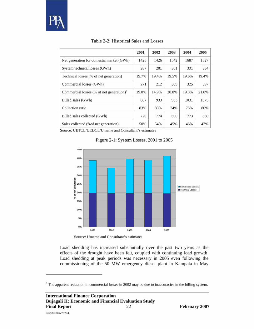
The data indicates that for the past five years billed sales revenue collected represents less than 50% of net generation. Technical losses are estimated to comprise about 4.5% for transmission and about 15% for distribution based on net energy generated. The resulting commercial or non-technical losses vary between 15% and almost 22% (in 2005), as shown in Figure 2-1.
7 Transmission losses for 2002 and 2003 have been adjusted to remove inconsistencies caused by metering problems.
International Finance Corporation Bujagali II: Economic and Financial Evaluation Study Final Report 22 February 2007 26/02/2007-20224
Table 2-2: Historical Sales and Losses
2001 2002 2003 2004 2005
Net generation for domestic market (GWh) 1425 1426 1542 1687 1827
System technical losses (GWh) 287 281 301 331 354
Technical losses (% of net generation) 19.7% 19.4% 19.5% 19.6% 19.4%
Commercial losses (GWh) 271 212 309 325 397
Commercial losses (% of net generation)8 19.0% 14.9% 20.0% 19.3% 21.8%
Billed sales (GWh) 867 933 933 1031 1075
Collection ratio 83% 83% 74% 75% 80%
Billed sales collected (GWh) 720 774 690 773 860
Sales collected (%of net generation) 50% 54% 45% 46% 47% Source: UETCL/UEDCL/Umeme and Consultant’s estimates
Figure 2-1: System Losses, 2001 to 2005
Source: Umeme and Consultant’s estimates
Load shedding has increased substantially over the past two years as the effects of the drought have been felt, coupled with continuing load growth. Load shedding at peak periods was necessary in 2005 even following the commissioning of the 50 MW emergency diesel plant in Kampala in May
8 The apparent reduction in commercial losses in 2002 may be due to inaccuracies in the billing system.
0%
5%
10%
15%
20%
25%
30%
35%
40%
45%
2001 2002 2003 2004 2005
% o
f net
gen
erat
ion
Commercial LossesTechnical Losses

International Finance Corporation Bujagali II: Economic and Financial Evaluation Study Final Report 23 February 2007 26/02/2007-20224
2005. Load shedding has increased from 1-2% of net generation in 2001/02 to 4-5% in 2004-05, as shown in Figure 2-2.
Figure 2-2: Details of Load Shedding, 2001 to 2005
Details of sales by tariff category are shown in Table 2-3. It should be noted that this data is not corrected for load shedding. Residential sales include tariff Code 10.1, which covers residential and small, single-phase, commercial premises metered at low voltage. Commercial sales include larger commercial consumers with a three-phase supply not exceeding 100 Amp, supplied at low voltage (Code 10.2/10.3). This category includes time of use (TOU) charging. The third category covers medium scale industrial consumers supplied at low voltage, three-phase up to 500 kVA (Code 20) and large scale industrial consumers supplied at 11 kV or 33 kV with a maximum demand between 500 kVA and 10 MVA. Street lighting (Code 50) is aggregated with the industrial consumption for the purposes of the demand forecast.
0
10
20
30
40
50
60
70
80
90
100
2001 2002 2003 2004 2005
GW
h
0%
1%
2%
3%
4%
5%
6%
% o
f net
gen
erat
ion
International Finance Corporation Bujagali II: Economic and Financial Evaluation Study Final Report 24 February 2007 26/02/2007-20224
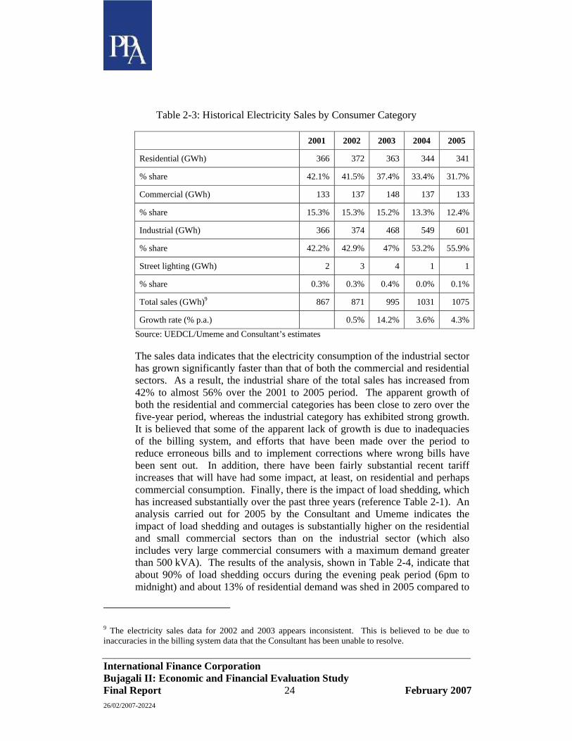
Table 2-3: Historical Electricity Sales by Consumer Category
2001 2002 2003 2004 2005
Residential (GWh) 366 372 363 344 341
% share 42.1% 41.5% 37.4% 33.4% 31.7%
Commercial (GWh) 133 137 148 137 133
% share 15.3% 15.3% 15.2% 13.3% 12.4%
Industrial (GWh) 366 374 468 549 601
% share 42.2% 42.9% 47% 53.2% 55.9%
Street lighting (GWh) 2 3 4 1 1
% share 0.3% 0.3% 0.4% 0.0% 0.1%
Total sales (GWh)9 867 871 995 1031 1075
Growth rate (% p.a.) 0.5% 14.2% 3.6% 4.3% Source: UEDCL/Umeme and Consultant’s estimates
The sales data indicates that the electricity consumption of the industrial sector has grown significantly faster than that of both the commercial and residential sectors. As a result, the industrial share of the total sales has increased from 42% to almost 56% over the 2001 to 2005 period. The apparent growth of both the residential and commercial categories has been close to zero over the five-year period, whereas the industrial category has exhibited strong growth. It is believed that some of the apparent lack of growth is due to inadequacies of the billing system, and efforts that have been made over the period to reduce erroneous bills and to implement corrections where wrong bills have been sent out. In addition, there have been fairly substantial recent tariff increases that will have had some impact, at least, on residential and perhaps commercial consumption. Finally, there is the impact of load shedding, which has increased substantially over the past three years (reference Table 2-1). An analysis carried out for 2005 by the Consultant and Umeme indicates the impact of load shedding and outages is substantially higher on the residential and small commercial sectors than on the industrial sector (which also includes very large commercial consumers with a maximum demand greater than 500 kVA). The results of the analysis, shown in Table 2-4, indicate that about 90% of load shedding occurs during the evening peak period (6pm to midnight) and about 13% of residential demand was shed in 2005 compared to
9 The electricity sales data for 2002 and 2003 appears inconsistent. This is believed to be due to inaccuracies in the billing system data that the Consultant has been unable to resolve.

International Finance Corporation Bujagali II: Economic and Financial Evaluation Study Final Report 25 February 2007 26/02/2007-20224
about 5% of industrial demand. The corresponding figure for the commercial category is 6%. This substantially higher load shedding in the residential sector has obviously impacted on the level of sales in 2005. Based on this analysis the unserved energy due principally to load shedding has been added back into the end-user sales figures, after allowing for losses. The resulting sales figures that formed the starting point for the demand forecast projections are shown in Table 2-5. The resulting average annual growth rate of total sales adjusted for unserved energy is 6.2% compared to 5.5% for the unadjusted total sales. It is interesting to note that residential sales do not appear to have increased over the period. Whilst part of this may be due to inaccuracies in the UEDCL billing records, the general consensus is that residential demand has been growing steadily. The conclusion that may be drawn, therefore, is that much of the increased consumption may be ‘hidden’ by increasing commercial losses.
Table 2-4: End-User Load Shedding Analysis for 2005
Item
Billed sales
Adjusted for system losses
Unsuppressed demand
GWh GWh % GWh GWhPeak consumption:Domestic/small commercial 170.3 48.5 22%Commercial 26.6 7.6 22%Industrial 99.8 28.4 18%Industrial (dedicated) supply 32.2 0
Total (peak) 328.9 84.5 20% 49.8 378.7
Non-peak consumption:Domestic/small commercial 170.3 2.5 1%Commercial 106.4 1.6 1%Industrial 361.9 5.3 1%Industrial (dedicated) supply 107.8 0
Total (non-peak) 746.4 9.39 1% 5.5 751.9
Total consumption:Domestic/small commercial 340.6 51.0 13%Commercial 133.0 9.1 6%Industrial 461.7 33.8 5%Industrial (dedicated) supply 140.0 0.0
Total (peak + non-peak) 1075.3 93.9 8% 55.3 1130.6
Load shed
Source: Umeme and Consultant’s analysis
The industrial dedicated supply covers large consumers that are supplied at HV on a ‘dedicated’ feeder that allows these consumers to remain on supply when other consumers in the area are subject to load shedding.
International Finance Corporation Bujagali II: Economic and Financial Evaluation Study Final Report 26 February 2007 26/02/2007-20224
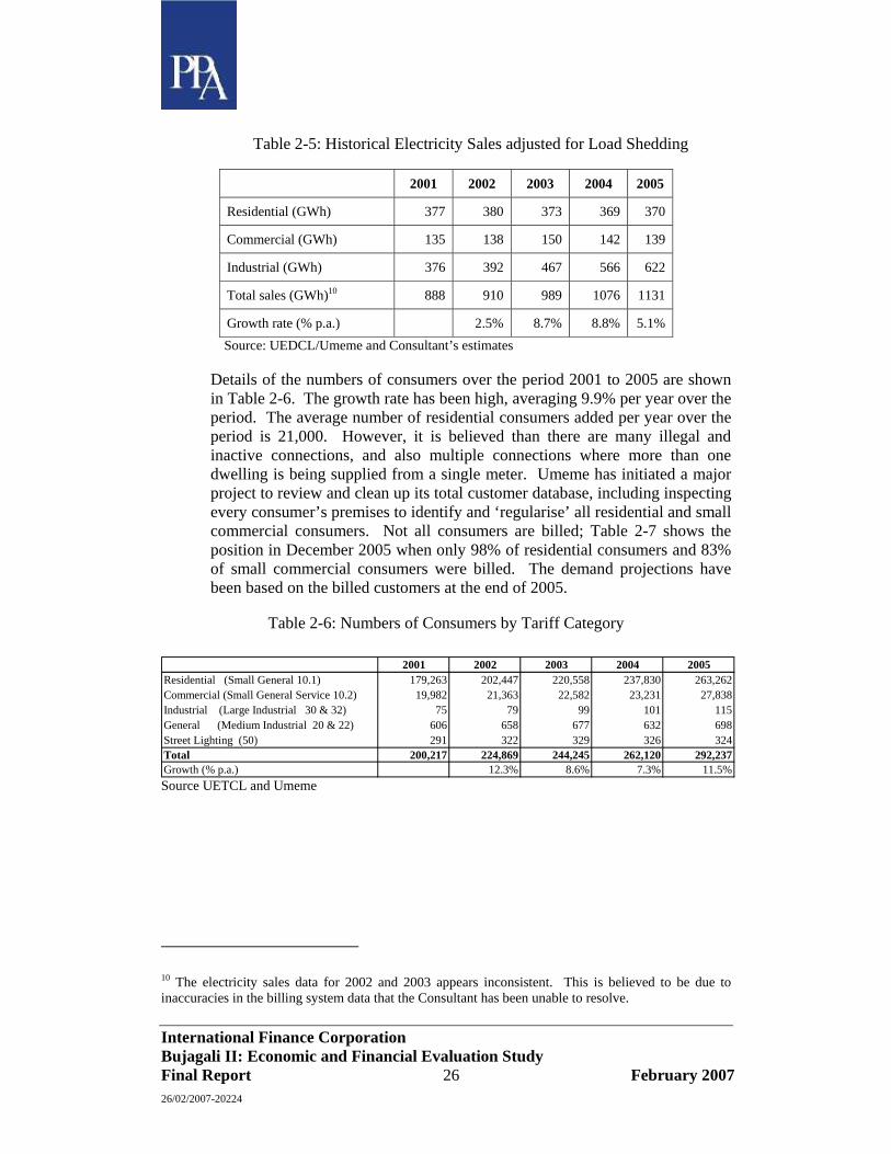
Table 2-5: Historical Electricity Sales adjusted for Load Shedding
2001 2002 2003 2004 2005
Residential (GWh) 377 380 373 369 370
Commercial (GWh) 135 138 150 142 139
Industrial (GWh) 376 392 467 566 622
Total sales (GWh)10 888 910 989 1076 1131
Growth rate (% p.a.) 2.5% 8.7% 8.8% 5.1% Source: UEDCL/Umeme and Consultant’s estimates
Details of the numbers of consumers over the period 2001 to 2005 are shown in Table 2-6. The growth rate has been high, averaging 9.9% per year over the period. The average number of residential consumers added per year over the period is 21,000. However, it is believed than there are many illegal and inactive connections, and also multiple connections where more than one dwelling is being supplied from a single meter. Umeme has initiated a major project to review and clean up its total customer database, including inspecting every consumer’s premises to identify and ‘regularise’ all residential and small commercial consumers. Not all consumers are billed; Table 2-7 shows the position in December 2005 when only 98% of residential consumers and 83% of small commercial consumers were billed. The demand projections have been based on the billed customers at the end of 2005.
Table 2-6: Numbers of Consumers by Tariff Category
Source UETCL and Umeme
10 The electricity sales data for 2002 and 2003 appears inconsistent. This is believed to be due to inaccuracies in the billing system data that the Consultant has been unable to resolve.
2001 2002 2003 2004 2005Residential (Small General 10.1) 179,263 202,447 220,558 237,830 263,262Commercial (Small General Service 10.2) 19,982 21,363 22,582 23,231 27,838Industrial (Large Industrial 30 & 32) 75 79 99 101 115General (Medium Industrial 20 & 22) 606 658 677 632 698Street Lighting (50) 291 322 329 326 324Total 200,217 224,869 244,245 262,120 292,237Growth (% p.a.) 12.3% 8.6% 7.3% 11.5%

International Finance Corporation Bujagali II: Economic and Financial Evaluation Study Final Report 27 February 2007 26/02/2007-20224
Table 2-7: Consumers Billed in December 2005
Source UETCL and Umeme
2.3 Methodology and Assumptions
Projections of electricity demand for the Ugandan interconnected system are required for the period up to 2020 for the analysis of the Bujagali project. The starting point for the projections is the 2005 demand, as discussed in Section 2.1. In this section, the methodology adopted for the demand forecast and the various assumptions are presented. A base case forecast, plus high and low sensitivity forecasts, are then developed based on projections for the economy, estimated new connections and assumptions on the future levels of system losses. Finally, forecasts are added covering committed exports to Tanzania and Rwanda.
The demand forecast has been built up from separate forecasts for each main consumer category based on a consistent set of economic and other assumptions, using actual data for 2005 as a starting point.
In the following sections, projections for the Ugandan economy are developed following a brief review of the recent performance of the economy.
2.4 Projections for Ugandan Economy
2.4.1 General
Projections of economic growth in Uganda are an integral component of the demand forecasting process. The Consultant’s projections are founded on short to medium term projections made by authorities on the Ugandan economy, such as MoFPED, BoU and the IMF. Since the Consultant’s projections have a considerably longer perspective than those prepared by these authorities, a view of the long-term prospects for the Ugandan economy has been taken. This view was formed on the basis of interviews with senior individuals at MoFPED, BoU and the IMF, and the review of recent reports prepared by MoFPED, BoU and the World Bank.
2.4.2 Overview of the Ugandan Economy
The Ugandan economy has enjoyed considerable stability for more than 10 years. Since the 1990/91 fiscal year, economic growth has averaged around 6.5% per year. In recent years, there has been a slight reduction in the average
Live Billed %Residential (Small General 10.1) 263,262 258,805 98%Commercial (Small General Service 10.2) 27,838 23,170 83%Industrial (Large Industrial 30 & 32) 115 115 100%General (Medium Industrial 20 & 22) 698 698 100%Street Lighting (50) 324 324 100%Total 292,237 283,112

International Finance Corporation Bujagali II: Economic and Financial Evaluation Study Final Report 28 February 2007 26/02/2007-20224
rate of growth, and the average for the past 5 years has been around 5.7%. In the most recent fiscal year (2004/05) GDP growth was 5.7%. It is, however, important to consider that population growth in Uganda is quite strong, at around 3.4%. Per capita GDP growth over the past 5 years is therefore around 2.3% per year.11
2.4.3 Projections
The GDP projections adopted for the base case demand forecast are taken from the current forecasts of the Ugandan economy agreed jointly between GoU, IMF and World Bank, adjusted for calendar years. These are summarised in Table 2-8. Projections provided by GoU cover financial year 2008/09 and we have extrapolated the projections up to 2011. It is assumed that the rates remain constant at the 2011 levels up to 2020.
It should be noted that the forecast overall GDP growth is lower than both the commercial and industrial GDP growth. This is due to the effect of the agriculture and informal sectors.
Table 2-8: Uganda GDP Projections
2006 2007 2008 2009 2010 2011-2020GDP at factor cost 5.75% 6.10% 6.45% 6.85% 6.45% 6.00%Commercial GDP growth 8.20% 7.25% 7.70% 8.35% 7.55% 7.90%Industrial GDP growth 6.15% 6.50% 6.85% 7.25% 6.85% 6.40%Source: Government of Uganda/IMF
2.5 Assumptions for Residential Sector
As discussed in Section 2.1, the growth in numbers of residential consumers has been strong, averaging almost 21,000 per year since 2001. The assumption adopted for new residential connections in the short term is 17,000 per year over the period 2006 to 2010 inclusive. This is assumed to comprise 12,000 by Umeme in urban and peri-urban areas, as per the target in their concession, plus a further 5,000 per year of grid-connected rural consumers from the RE programmes being implemented by the REA and UEDCL. Umeme is not expecting to connect more consumers than they are committed to in their concession in view of the shortages of generation and high tariffs that are likely to be experienced until Bujagali comes into service. From 2011 to 2020, it is assumed that the numbers of connections will increase following the end to generation capacity constraints, which will trigger an increase in the rate of connections, both urban and rural. Over this period it is assumed that 25,000 new residential consumers will be connected each year, including both urban and rural connections.
11 In the 12 years to 2002, the population of Uganda grew by 7.7 million, to stand at 24.4 million.
International Finance Corporation Bujagali II: Economic and Financial Evaluation Study Final Report 29 February 2007 26/02/2007-20224
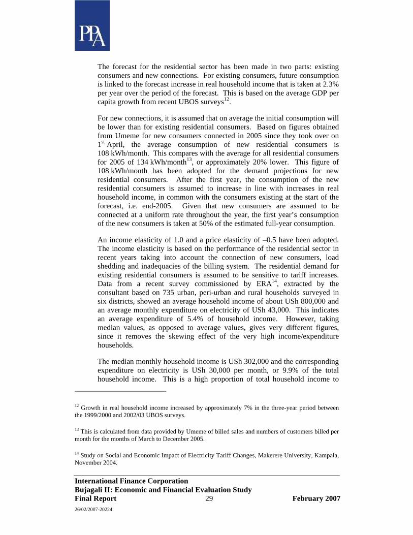
The forecast for the residential sector has been made in two parts: existing consumers and new connections. For existing consumers, future consumption is linked to the forecast increase in real household income that is taken at 2.3% per year over the period of the forecast. This is based on the average GDP per capita growth from recent UBOS surveys12.
For new connections, it is assumed that on average the initial consumption will be lower than for existing residential consumers. Based on figures obtained from Umeme for new consumers connected in 2005 since they took over on 1st April, the average consumption of new residential consumers is 108 kWh/month. This compares with the average for all residential consumers for 2005 of 134 kWh/month13, or approximately 20% lower. This figure of 108 kWh/month has been adopted for the demand projections for new residential consumers. After the first year, the consumption of the new residential consumers is assumed to increase in line with increases in real household income, in common with the consumers existing at the start of the forecast, i.e. end-2005. Given that new consumers are assumed to be connected at a uniform rate throughout the year, the first year’s consumption of the new consumers is taken at 50% of the estimated full-year consumption.
An income elasticity of 1.0 and a price elasticity of –0.5 have been adopted. The income elasticity is based on the performance of the residential sector in recent years taking into account the connection of new consumers, load shedding and inadequacies of the billing system. The residential demand for existing residential consumers is assumed to be sensitive to tariff increases. Data from a recent survey commissioned by ERA14, extracted by the consultant based on 735 urban, peri-urban and rural households surveyed in six districts, showed an average household income of about USh 800,000 and an average monthly expenditure on electricity of USh 43,000. This indicates an average expenditure of 5.4% of household income. However, taking median values, as opposed to average values, gives very different figures, since it removes the skewing effect of the very high income/expenditure households.
The median monthly household income is USh 302,000 and the corresponding expenditure on electricity is USh 30,000 per month, or 9.9% of the total household income. This is a high proportion of total household income to
12 Growth in real household income increased by approximately 7% in the three-year period between the 1999/2000 and 2002/03 UBOS surveys.
13 This is calculated from data provided by Umeme of billed sales and numbers of customers billed per month for the months of March to December 2005.
14 Study on Social and Economic Impact of Electricity Tariff Changes, Makerere University, Kampala, November 2004.
International Finance Corporation Bujagali II: Economic and Financial Evaluation Study Final Report 30 February 2007 26/02/2007-20224
spend on electricity. These figures indicate that the demand of the majority of residential consumers is relatively highly elastic and therefore a price elasticity of –0.5 has been adopted for the demand forecast. The median figures also indicate an average consumption of about 123 kWh/month at current early-2006 tariff levels, compared with an average of 134 kWh/month based on the Umeme billing data for March to December 200515. Applying the 24% tariff increase in April 2005 to the median figure, and using price elasticity of –0.5, gives an average consumption of 138 kWh per month, which is close to the ‘actual’ figure from Umeme for 2005. It is considered justifiable therefore to adopt a price elasticity of demand for the residential sector of –0.5. It should also be noted that the residential consumer category (tariff code 10.1) also includes small shops and other small commercial premises. It has been assumed that any impact of these consumers on the above analysis will be small. This assumption is supported by the analysis of willingness to pay for electricity which indicates that, the price elasticity of demand at the marginal residential tariff (point P2Q2 on the income compensated demand curve) is -0.45 (see Appendix E.1.3).
It is useful to consider that multiple households are actually being served by the average Umeme residential connection. Statistics Norway consultants’ analysis of 2002 UBOS survey data found that 451,000 households were connected to mains electricity, whereas 2005 Umeme data indicated just 255,000 official residential connections. This suggests that there are approximately 1.8 households supplied by each residential connection. When this information is applied to the average residential customer, the proportion of household income spent on electricity is reduced to just 3.2%, which is much closer to expectations.
It is also useful to consider whether electricity will still be affordable in 2011, with the tariff trajectory that is expected. Assuming a 2.3% real annual income growth over the 6 years between 2005 and 2011 suggests that the average residential income will grow by 14.6% from US$ 3,952 to US$ 4,529 per year and, assuming an income elasticity of demand of 1.0, electricity consumption will also grow by 14.6% from 134 kWh/month to 154 kWh/month. With a 2011 tariff of 23.0 US¢/kWh, in 2006 money, the implicit expenditure on electricity increases to US$ 35.4 per month, or US$ 425 per year. This represents 9.4% of household income, on the basis of a single household per connection, or 5.2% on the basis of 1.8 households per connection. The Consultant considers that 5.2% is towards the upper end of the range of expectations for the proportion of household income expended on electricity for non-cooking purposes.
15 This is higher than the average residential consumption per consumer on which the demand forecast is based since the demand forecast uses the year-end consumer numbers whereas the Umeme average consumption data is based on average month-by-month billing data.

International Finance Corporation Bujagali II: Economic and Financial Evaluation Study Final Report 31 February 2007 26/02/2007-20224
2.6 Assumptions for Commercial and Industrial Sectors
The demand projections for the commercial and industrial sectors are based on GDP projections for the services and industrial sectors presented in Section 2.4.3. The following assumptions have been adopted for demand and prices elasticities for these sectors:
Commercial: GDP elasticity 1.0 Price elasticity -0.3 Industrial: GDP elasticity 1.3 Price elasticity -0.1
These figures have been derived from an analysis of historical GDP and electricity sales for these sectors. For the commercial sector an analysis was carried out for the period 1977-2003. The average growth in electricity sales was 6.75 and the average growth in GDP was 6.8%, giving a GDP elasticity of demand for the sector of 0.99. Therefore, a value of 1.0 has been adopted. The analysis was only made for the period up to 2003 in view of suspected problems with the billing data that the Consultant was unable to resolve.
A similar analysis was made for the industrial sector. In this case, the period 1997 to 2005 was adopted and a GDP elasticity of demand of 1.38 was obtained. A value of 1.3 has been adopted for the demand projections.
The price elasticities adopted were based on more judgemental arguments. It is considered that the demand of the industrial sector is highly inelastic due to the high cost of alternative sources of generation and the high establishment costs of auto-generation. A low price elasticity of –0.1 has therefore been adopted for the demand projections. For the commercial sector it was also felt that the demand is relatively inelastic. However, it was also considered that the commercial demand would be less price elastic than the residential sector. For the commercial sector, a price elasticity of –0.3 has therefore been adopted for the demand projections.
2.7 Revenue Collection
The present collection ratio for energy billed is 80% and Umeme is committed under the concession agreement to improving the ratio to 92.5% by 2008. The demand forecast is based on achieving 90% by 2008 and 97.55 by 2011, remaining constant thereafter. A price elasticity of demand on improved revenue collections of -0.30 has been adopted, implying that there will be 0.3% reduction in demand for each perceived 1% price increase as a result of Umeme’s improved collection of billed revenue.
International Finance Corporation Bujagali II: Economic and Financial Evaluation Study Final Report 32 February 2007 26/02/2007-20224
2.8 Tariff Assumptions
Electricity tariffs increased twice in 2005, in April and October by a total of 24% on average and by 37% in June 2006. ERA increased tariffs by a further 42% on average in November 200616 in view of the rising cost of the thermal generation and the planned additional short term emergency thermal plant. The capacity costs of the future short term thermal are expected to be covered by the World Bank, under IDA funding and GoU is expected to waive the fuel duty and further subsidise the fuel cost. However, at the time of writing this report, the amount of the subsidy, and therefore the amount that would have to be passed through to consumers through the tariff, is not known.
A separate short-term study has been commissioned by the World Bank17 to evaluate the short term thermal generation proposed program. Based on the findings of this study the following real increases in average end-user tariffs will be required over the period up to the commissioning of Bujagali in 2011:
2006 +37% 2007 +45% 2008 +15% 2009 0% 2010 0% 2011 -15%
The above tariffs are based on the proposed short term thermal programme, including an additional 150 MW firm of generating plant – 100 MW leased high-speed diesels and 50 MW firm of medium speed diesel plant burning heavy fuel oil (HFO)18. The tariff projections also assume that there would be continuing direct budgetary support to the sector, plus IDA support of a further US$ 175 million.
The revised demand forecast used for developing the least cost development programme for the Ugandan system has been based on the above tariff assumptions. The financial analysis based on the least cost programme will provide a forecast of the tariffs required to meet the financial requirements of the electricity sector. If the calculated tariffs are no greater than the tariffs underlying the demand forecast, the expected demand and supply conditions
16 This latest increase was not known when the Consultant finalized the demand forecast, but is close to the assumed tariff increase in 2007.
17 Assessment of Short Term Generation Requirements in Uganda, Draft Report, February 2006, Power Planning Associates
18 This is the plant that is to be developed as an IPP on a BOT basis, with ownership passing to the government after 6 years of operation.
International Finance Corporation Bujagali II: Economic and Financial Evaluation Study Final Report 33 February 2007 26/02/2007-20224
would be not far from equilibrium. However, if the tariffs calculated for the investment plan based on the original tariff assumptions end-up exceeding the latter, then the forecast and least cost plan will be revised based on the calculated tariffs. This process will be re-iterated until there is approximate coherence between prices, demand and supply.
2.9 Assumptions on Reduction of System Losses
As discussed in Section 2.1, system losses on the Ugandan system are currently very high. It is estimated that losses in 2005 were 41.1% of net generation on an energy basis, made up as follows:
Transmission losses 4.4% Distribution losses 16.0% Commercial losses 20.7%
The commercial loss percentage does not include for consumption that is billed but not paid which is allowed-for separately in the demand forecast.
Based on discussions with Umeme staff the estimated breakdown of the distribution technical losses is as follows:
11 & 33 kV distribution networks 6% LV distribution networks 10% (including a substantial contribution from unbalanced loadings on LV networks) Umeme has engaged Norconsult to investigate the present level of losses and to make proposals for loss reduction. Based on these findings and additional discussions with Umeme, the consultant estimates the following current (2006) system losses, expressed as percentages of net generation: Technical losses: Transmission 4.0% Distribution 16% Sub-total 20%
Commercial losses 19%
Total losses 39%
The Umeme capital investment programme for the period to 2010 includes a budget of US$ 56.6 million to address the above issues and it is considered that reduction of about 4% should be possible over the next seven years, to 2012. Allowing for a modest decrease in transmission losses from 4.4% to 4.0%, the estimated target technical loss level for the base demand forecast is 16%, comprising 4% transmission losses and 12% distribution losses. However, there is a strong incentive for Umeme to exceed these loss targets
International Finance Corporation Bujagali II: Economic and Financial Evaluation Study Final Report 34 February 2007 26/02/2007-20224
Forecasting attainable levels of commercial losses is more difficult. The current level of commercial losses is very high and is not justified in a well-managed distribution utility. Umeme fully appreciates this and is committed under the concession agreement to reduce losses by 0.85% per year for the next seven years from a starting level of 33%. Thus, the committed level of distribution losses in 2011 is 28%, from the 2005 level estimated at 36.7%19. In principle, it should be possible to reduce commercial losses to virtually zero by cutting out theft, faulty and inaccurate metering and meter reading irregularities. However, in most developing countries such as Uganda, the level of commercial losses varies widely and depends to a large extent on the attitude of the utility and the law enforcement authorities to theft of electricity and willingness to address the issues and take the necessary actions to improve metering and billing processes, and treating those found to be engaging in theft of electricity as criminals. All kWhs that are lost or stolen can be either converted directly into sales revenue, or alternatively, once regularised, will drop out of the system and therefore represent a direct saving on Umeme’s purchases from UETCL.
There are strong indications already that Umeme is taking commercial loss reduction extremely seriously. The following initiatives have already been taken or are in process:
• Declaration of an amnesty whereby persons stealing electricity who report to Umeme prior to 16 February 2006 will not be prosecuted. Those found to be receiving electricity illegally thereafter will have their connection physically removed and will be prosecuted.
• Establishing a dedicated loss reduction unit. This unit will be undertaking a comprehensive customer and low voltage verification and database clean-up, including house to house surveys of Umeme’s small residential and commercial customers. The project will be carried out initially in Kampala city where there are estimated to be approximately 150,000 legal connections and +/-30,000 illegal connections. It is estimated that the project will take two years, starting in Q2-2006. Meanwhile, Umeme has carried out checks on the 890 customers in tariff codes 20 and 30.
• Un-metered connections have already been reduced from 19,000 to 500. Umeme is aware that there are a further 10,000 consumers are connected but not registered in the billing system.
19 Loss targets have been restated as part of Umeme’s negotiations on the concession agreement with GoU in November 2006. For an interim period losses are set quarterly based on the actual losses for the previous quarter less 1%. The interim period is estimated to last until Bujagali is commissioned.

International Finance Corporation Bujagali II: Economic and Financial Evaluation Study Final Report 35 February 2007 26/02/2007-20224
• In parallel with the LV and customer verification programme, Umeme has gone out to tender for a new state-of-the-art billing system. The database for the new billing system will be populated based on the results of the customer verification programme.
There is no doubt that if the above programmes are carried through with diligence and determination, and Umeme’s efforts are supported by the courts in terms of imposing penalties that present strong deterrents, then this programme could have a very substantial impact in bringing down the current high levels of commercial losses to levels that are consistent with a well managed distribution utility. Residual levels of commercial losses of between 2% and 6% should be achievable, with a base case demand forecast assumption of 5%, by 2012. The future levels of technical and commercial losses for the base case forecast are set out in Table 2-9. Loss levels are assumed to remain constant at the 2012 levels up to 2020.
Table 2-9: Forecasts of Technical and Commercial Losses
2005 2006 2007 2008 2009 2010 2011 2012Technical losses 19.4% 20.0% 19.5% 18.8% 18.1% 17.4% 16.7% 16.0%Commercial losses 21.7% 19.0% 17.0% 15.0% 12.0% 9.0% 7.0% 5.0%Total losses 41.1% 39.0% 36.5% 33.8% 30.1% 26.4% 23.7% 21.0%Source: Consultant’s estimates.
Consideration has been given to the impact of commercial loss reduction on end-user sales. Following further discussions with Umeme, it has been estimated that 70% of commercial losses will be converted into billed sales and the remaining 30% will drop out of the system. This assumption has been adopted in deriving the base forecast and the high/low sensitivity forecasts.
2.10 Electricity Exports
Uganda has on-going agreement with Kenya for export/import of non-firm power over the existing double circuit 132 kV line between Owen Falls substation and Lessos. At present, neither country has any significant spare capacity to export, although the systems are normally operated with the 132 kV line connected, as it assists both transmission operators to meet reactive power requirements and to maintain system stability. UETCL was in negotiations with KPLC, Kenya to export 50 MW of firm power, and up to 80 MW non-firm, following the commissioning of Bujagali for a period of 20 years, with penalties for non-delivery, at a tariff of 5.9 US¢/kWh. Under the current agreement with Kenya, the tariff is 4.5 US¢/kWh plus the average cost of fuel for the previous month (based on the Aggreko plant). There are also plans to extend the proposed double circuit 220 kV line to be constructed between Kiwanga substation, near Kampala, and Owen Falls to Lessos in Kenya, via Tororo. This would increase the potential export capacity to Kenya to 360 MW. The Kenyan government has indicated a willingness to purchase additional power from Uganda. However, at the time this report was

International Finance Corporation Bujagali II: Economic and Financial Evaluation Study Final Report 36 February 2007 26/02/2007-20224
prepared, it is understood that no contract has been signed between UETCL and KPLC for the export of power to Kenya and therefore the analysis in this report is based on the forecast Uganda demand, plus the limited exports to Tanzania and Rwanda, as discussed below.
Uganda has an agreement with Tanzania to export power to the Bukoba area close to the Ugandan border. Bukoba is a sugar growing area and is isolated from the Tanesco grid. The peak demand was 7.1 MW in 2005, and the total energy supplied was 32 GWh.
Finally, there is a weak (33 kV) interconnection between Kabale and Rwanda. About 1 GWh of energy was imported in 2005.
It is understood that there are no plans for a substantial increase in exports to Tanzania and Rwanda. For the purposes of the demand forecast it has been assumed that the exports to Bukoba and Rwanda increase at 5-6% per year to cater for natural load growth.
2.11 Load Forecast Results and Sensitivity Scenarios
The base case forecast is summarised in Table 2-10 and the high and low sensitivity scenarios in Table 2-11.
The high and low sensitivity forecasts are based on the following assumptions:
New residential connections High: +20,000 per year to 2010 and +30,000 per year thereafter; Low: +12,000 per year to 2010 and +17,000 per year thereafter.
Increase in real household income High: base value +1%; Low: base value -1.5%
Commercial and industrial GDP High: base value +2%; Low: base value -3%.
Tariffs As base forecast. Technical losses As for base forecast Commercial losses As for base forecast
The skewed assumptions for the household income and commercial and industrial GDP estimates in the high/low sensitivity forecasts reflect the vulnerability of Uganda to external economic shocks over which Uganda has no control.
All other assumptions are the same as the base forecast.

International Finance Corporation Bujagali II: Economic and Financial Evaluation Study Final Report 37 February 2007 26/02/2007-20224
The forecasts are shown graphically in Figure 2-3 for peak demand (MW), Figure 2-4 for net generation (GWh) and Figure 2-5 for sales (GWh). The peak demand and net generation values include committed exports to Tanzania and Rwanda.
Figure 2-3: Peak Demand Forecasts (including committed exports) – MW net
0
200
400
600
800
1000
1200
2005 2006 2007 2008 2009 2010 2011 2012 2013 2014 2015 2016 2017 2018 2019 2020
MW
net Base
HighLow
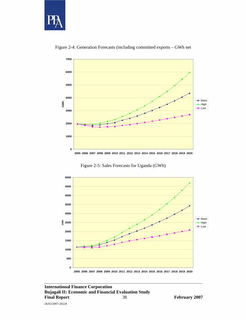
International Finance Corporation Bujagali II: Economic and Financial Evaluation Study Final Report 38 February 2007 26/02/2007-20224
Figure 2-4: Generation Forecasts (including committed exports – GWh net
0
1000
2000
3000
4000
5000
6000
7000
2005 2006 2007 2008 2009 2010 2011 2012 2013 2014 2015 2016 2017 2018 2019 2020
GW
h BaseHighLow
Figure 2-5: Sales Forecasts for Uganda (GWh)
0
500
1000
1500
2000
2500
3000
3500
4000
4500
5000
2005 2006 2007 2008 2009 2010 2011 2012 2013 2014 2015 2016 2017 2018 2019 2020
GW
h
BaseHighLow
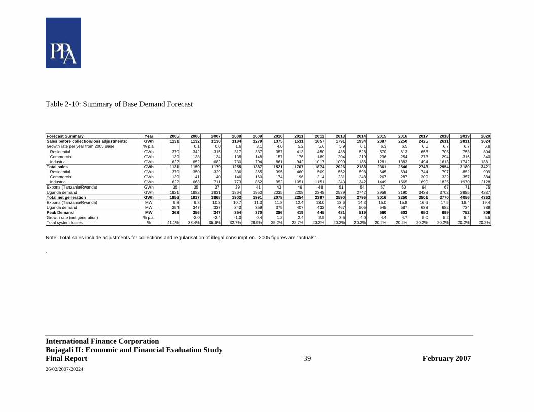
International Finance Corporation Bujagali II: Economic and Financial Evaluation Study Final Report 39 February 2007 26/02/2007-20224
Table 2-10: Summary of Base Demand Forecast
Forecast Summary Year 2005 2006 2007 2008 2009 2010 2011 2012 2013 2014 2015 2016 2017 2018 2019 2020Sales before collection/loss adjustments: GWh 1131 1132 1130 1184 1279 1375 1531 1657 1791 1934 2087 2250 2425 2611 2811 3024Growth rate per year from 2005 Base % p.a. 0.1 0.0 1.6 3.1 4.0 5.2 5.6 5.9 6.1 6.3 6.5 6.6 6.7 6.7 6.8 Residential GWh 370 342 315 317 337 357 413 450 488 528 570 613 658 705 753 804 Commercial GWh 139 138 134 138 148 157 176 189 204 219 236 254 273 294 316 340 Industrial GWh 622 652 682 730 794 861 942 1017 1099 1186 1281 1383 1494 1613 1742 1881Total sales GWh 1131 1159 1179 1255 1387 1521 1707 1874 2026 2188 2361 2546 2743 2954 3180 3421 Residential GWh 370 350 329 336 365 395 460 509 552 598 645 694 744 797 852 909 Commercial GWh 139 141 140 146 160 174 196 214 231 248 267 287 309 332 357 384 Industrial GWh 622 668 711 773 862 952 1051 1151 1243 1342 1449 1565 1690 1825 1970 2128Exports (Tanzania/Rwanda) GWh 35 35 37 39 41 43 46 48 51 54 57 60 64 67 71 75Uganda demand GWh 1921 1882 1831 1864 1950 2035 2208 2348 2539 2742 2959 3190 3438 3702 3985 4287Total net generation GWh 1956 1917 1868 1903 1991 2078 2254 2397 2590 2796 3016 3250 3501 3770 4056 4363Exports (Tanzania/Rwanda) MW 9.8 9.8 10.3 10.7 11.3 11.8 12.4 13.0 13.6 14.3 15.0 15.8 16.6 17.5 18.4 19.4Uganda demand MW 354 347 337 343 359 375 407 432 467 505 545 587 633 682 734 789Peak Demand MW 363 356 347 354 370 386 419 445 481 519 560 603 650 699 752 809Growth rate (net generation) % p.a. -2.0 -2.4 -1.0 0.4 1.2 2.4 2.9 3.5 4.0 4.4 4.7 5.0 5.2 5.4 5.5Total system losses % 41.1% 38.4% 35.6% 32.7% 28.9% 25.2% 22.7% 20.2% 20.2% 20.2% 20.2% 20.2% 20.2% 20.2% 20.2% 20.2%
Note: Total sales include adjustments for collections and regularisation of illegal consumption. 2005 figures are “actuals”.
.

International Finance Corporation Bujagali II: Economic and Financial Evaluation Study Final Report 40 February 2007 26/02/2007-20224
Table 2-11: Summary of High and Low Demand Forecasts
High forecast Forecast Summary Year 2005 2006 2007 2008 2009 2010 2011 2012 2013 2014 2015 2016 2017 2018 2019 2020Sales before collection/loss adjustments: GWh 1131 1155 1179 1263 1393 1530 1740 1924 2125 2344 2584 2845 3131 3442 3783 4156Growth rate per year from 2005 Base % p.a. 2.2 2.1 3.7 5.4 6.2 7.4 7.9 8.2 8.4 8.6 8.8 8.9 8.9 9.0 9.1 Residential GWh 370 347 326 334 361 389 457 508 561 617 677 739 805 875 948 1025 Commercial GWh 139 141 139 145 159 172 197 215 236 259 283 311 340 373 408 447 Industrial GWh 622 667 715 783 873 968 1086 1201 1328 1468 1623 1795 1985 2195 2427 2683Total sales GWh 1131 1183 1231 1338 1511 1692 1940 2176 2404 2652 2923 3218 3541 3894 4280 4702 Residential GWh 370 356 340 354 391 430 510 575 635 698 766 836 911 990 1073 1160 Commercial GWh 139 144 145 154 172 191 219 244 267 293 321 351 385 422 462 506 Industrial GWh 622 684 746 830 947 1071 1211 1358 1502 1661 1836 2031 2245 2483 2745 3036Exports (Tanzania/Rwanda) GWh 35.0 35.0 36.9 39.0 41.1 43.4 45.8 48.4 51.1 54.0 57.1 60.3 63.7 67.4 71.3 75.3Uganda demand GWh 1921 1921 1910 1987 2124 2264 2510 2728 3012 3323 3663 4033 4438 4880 5364 5892Total Net Generation GWh 1956 1956 1947 2026 2165 2307 2555 2776 3064 3377 3720 4094 4502 4948 5435 5968Exports (Tanzania/Rwanda) MW 9.8 9.8 10.3 10.7 11.3 11.8 12.4 13.0 13.6 14.3 15.0 15.8 16.6 17.5 18.4 19.4Uganda demand MW 354 354 352 366 391 417 462 502 555 612 674 743 817 899 988 1085Peak Demand MW 363 363 362 377 402 429 474 515 568 626 689 758 834 916 1006 1104Growth rate (net generation) % p.a. 0.0 -0.3 1.1 2.6 3.3 4.6 5.1 5.8 6.3 6.7 7.0 7.2 7.4 7.6 7.8Total system losses % 41.1% 38.4% 35.6% 32.7% 28.9% 25.2% 22.7% 20.2% 20.2% 20.2% 20.2% 20.2% 20.2% 20.2% 20.2% 20.2%
Low forecast
Forecast Summary Year 2005 2006 2007 2008 2009 2010 2011 2012 2013 2014 2015 2016 2017 2018 2019 2020Sales before collection/loss adjustments: GWh 1131 1096 1058 1072 1120 1165 1254 1312 1371 1433 1496 1561 1629 1699 1771 1845Growth rate per year from 2005 Base % p.a. -3.0 -3.3 -1.8 -0.2 0.6 1.7 2.1 2.4 2.7 2.8 3.0 3.1 3.2 3.3 3.3 Residential GWh 370 334 298 292 301 311 349 369 389 409 430 450 472 493 515 537 Commercial GWh 139 134 126 126 132 137 149 156 163 170 178 186 195 203 213 222 Industrial GWh 622 628 633 654 686 717 757 788 820 854 889 925 963 1002 1043 1086Total sales GWh 1131 1123 1104 1136 1214 1288 1399 1484 1551 1621 1692 1766 1843 1922 2003 2088 Residential GWh 370 342 311 309 327 344 389 417 440 463 486 510 533 558 582 607 Commercial GWh 139 137 132 134 143 151 166 176 184 192 201 210 220 230 241 252 Industrial GWh 622 644 661 693 744 793 844 891 927 966 1005 1046 1089 1134 1180 1228Exports (Tanzania/Rwanda) GWh 35.0 35.0 36.9 39.0 41.1 43.4 45.8 48.4 51.1 54.0 57.1 60.3 63.7 67.4 71.3 75.3Uganda demand GWh 1921 1823 1714 1687 1708 1723 1809 1860 1944 2031 2121 2214 2309 2408 2511 2616Total Net Generation GWh 1956 1858 1751 1726 1749 1767 1855 1908 1995 2085 2178 2274 2373 2476 2582 2692Exports (Tanzania/Rwanda) MW 9.8 9.8 10.3 10.7 11.3 11.8 12.4 13.0 13.6 14.3 15.0 15.8 16.6 17.5 18.4 19.4Uganda demand MW 354 336 316 311 314 317 333 342 358 374 390 408 425 443 462 482Peak Demand MW 363 346 326 321 326 329 346 355 372 388 406 423 442 461 481 501Growth rate (net generation) % p.a. -5.1 -5.5 -4.2 -2.9 -2.1 -1.0 -0.5 0.2 0.6 1.0 1.3 1.5 1.8 1.9 2.1Total system losses % 41.1% 38.4% 35.6% 32.7% 28.9% 25.2% 22.7% 20.2% 20.2% 20.2% 20.2% 20.2% 20.2% 20.2% 20.2% 20.2%
Note: Total sales include adjustments for collections and regularisation of illegal consumption. 2005 figures are “actuals”.
International Finance Corporation Bujagali II: Economic and Financial Evaluation Study Final Report 41 February 2007 26/02/2007-20224
3 Hydrology and Energy Generation of Hydro Power Plants
3.1 Introduction
This chapter covers a broad range of issues including not only hydrology itself, and the evaluation of the hydrological resources of Lake Victoria, but also reservoir operation studies and hydro energy generation calculations that constitute essential data for the least-cost expansion plans modelling. Clarification on the causes of the recent drop in lake level is also addressed in this chapter. All these issues address the requirements of Task B of the Terms of Reference “Hydrological Performance of Lake Victoria”.
Owing to the variety and volume of the analysis that was required to address all these issues, the details of this part of the study are presented in a specific Appendix “Hydrology and Energy Generation of Hydro Power Plants”.
This appendix includes the following parts.
• Analysis of Lake Victoria Outflow, Net Basin Supply and Rainfall
• Analysis of recent departure from the Agreed Curve Period 1900 - 2001
• Discussion of Issues Related to Climatic Change
• Hydrological Scenarios
• Lake Operation Modelling
• Evaluation of Power and Energy Generation of Hydro Power Plants
The ultimate objective of the analysis is to assess the hydrological performance of Lake Victoria, by deriving the longest reliable series of Net Basin Supply (or net inflow into the lake) that should be used for the evaluation of energy generation of the existing and foreseen hydro power projects on the Victoria Nile, downstream of Owen Falls.
In addition to this main objective, the causes for the recent drop in lake level were also investigated. The analysis of the causes of this event is helpful in understanding the key drivers in the hydrological performance of Lake Victoria.
3.2 Lake Victoria Net Basin Supply
The Net Basin Supply (NBS) of Lake Victoria is defined as the net flow of water into the lake that is available at any time either to be released from the lake (at Owen Falls, only outlet of the lake) or to re-fill the lake. The NBS is
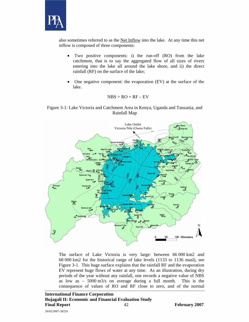
International Finance Corporation Bujagali II: Economic and Financial Evaluation Study Final Report 42 February 2007 26/02/2007-20224
also sometimes referred to as the Net Inflow into the lake. At any time this net inflow is composed of three components:
• Two positive components: i) the run-off (RO) from the lake catchment, that is to say the aggregated flow of all sizes of rivers entering into the lake all around the lake shore, and ii) the direct rainfall (RF) on the surface of the lake;
• One negative component: the evaporation (EV) at the surface of the lake.
NBS = RO + RF – EV
Figure 3-1: Lake Victoria and Catchment Area in Kenya, Uganda and Tanzania, and Rainfall Map
The surface of Lake Victoria is very large: between 66 000 km2 and 68 000 km2 for the historical range of lake levels (1133 to 1136 masl), see Figure 3-1. This huge surface explains that the rainfall RF and the evaporation EV represent huge flows of water at any time. As an illustration, during dry periods of the year without any rainfall, one records a negative value of NBS as low as – 5000 m3/s on average during a full month. This is the consequence of values of RO and RF close to zero, and of the normal
Lake Outlet Victoria Nile (Owen Falls)
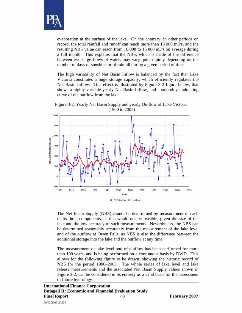
International Finance Corporation Bujagali II: Economic and Financial Evaluation Study Final Report 43 February 2007 26/02/2007-20224
evaporation at the surface of the lake. On the contrary, in other periods on record, the total rainfall and runoff can reach more than 15 000 m3/s, and the resulting NBS value can reach from 10 000 to 15 000 m3/s on average during a full month. This explains that the NBS, which is made of the difference between two large flows of water, may vary quite rapidly depending on the number of days of sunshine or of rainfall during a given period of time.
The high variability of Net Basin Inflow is balanced by the fact that Lake Victoria constitutes a huge storage capacity, which efficiently regulates the Net Basin Inflow. This effect is illustrated by Figure 3-2 figure below, that shows a highly variable yearly Net Basin Inflow, and a smoothly undulating curve of the outflow from the lake.
Figure 3-2: Yearly Net Basin Supply and yearly Outflow of Lake Victoria (1900 to 2005)
The Net Basin Supply (NBS) cannot be determined by measurement of each of its three components, as this would not be feasible, given the size of the lake and the low accuracy of such measurements. Nevertheless, the NBS can be determined reasonably accurately from the measurement of the lake level and of the outflow at Owen Falls, as NBS is also the difference between the additional storage into the lake and the outflow at any time.
The measurement of lake level and of outflow has been performed for more than 100 years, and is being performed on a continuous basis by DWD. This allows for the following figure to be drawn, showing the historic record of NBS for the period 1900–2005. The whole series of lake level and lake release measurements and the associated Net Basin Supply values shown in Figure 3-2, can be considered in its entirety as a valid basis for the assessment of future hydrology.
-500
0
500
1 000
1 500
2 000
2 500
3 000
1900 1910 1920 1930 1940 1950 1960 1970 1980 1990 2000 2010
Year
NB
S an
d O
utflo
w (m
3/s)
NBS (m3/s) Outflow
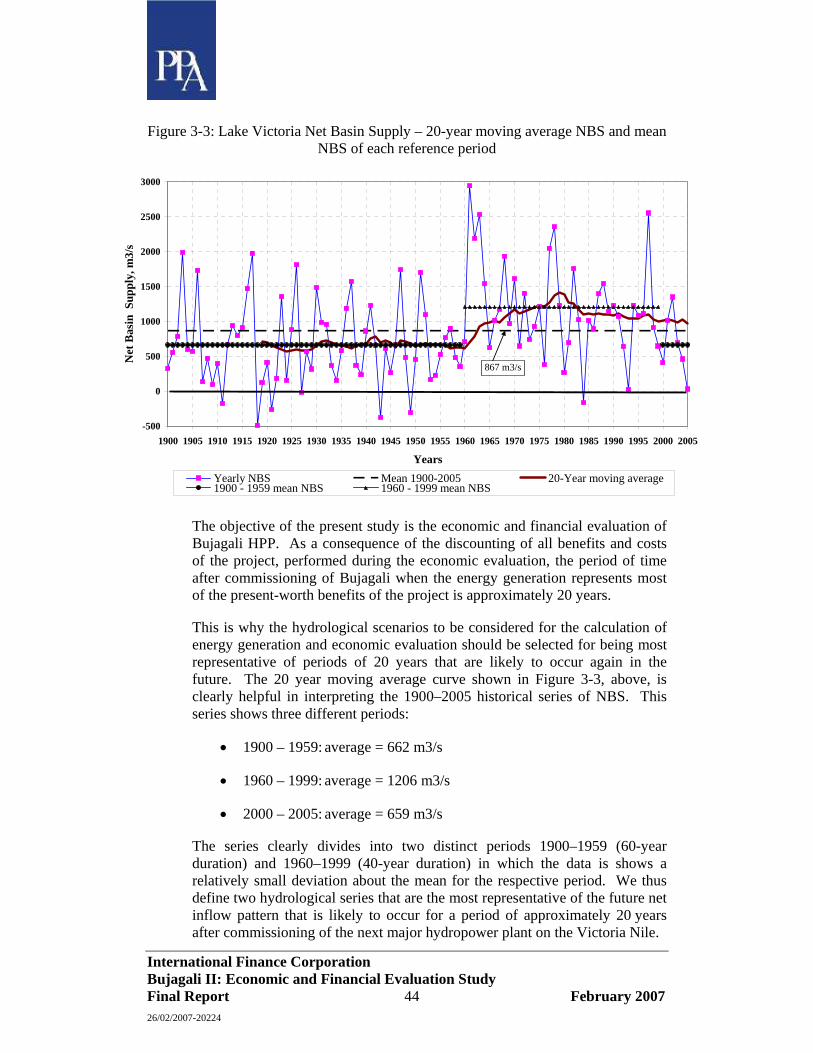
International Finance Corporation Bujagali II: Economic and Financial Evaluation Study Final Report 44 February 2007 26/02/2007-20224
Figure 3-3: Lake Victoria Net Basin Supply – 20-year moving average NBS and mean NBS of each reference period
The objective of the present study is the economic and financial evaluation of Bujagali HPP. As a consequence of the discounting of all benefits and costs of the project, performed during the economic evaluation, the period of time after commissioning of Bujagali when the energy generation represents most of the present-worth benefits of the project is approximately 20 years.
This is why the hydrological scenarios to be considered for the calculation of energy generation and economic evaluation should be selected for being most representative of periods of 20 years that are likely to occur again in the future. The 20 year moving average curve shown in Figure 3-3, above, is clearly helpful in interpreting the 1900–2005 historical series of NBS. This series shows three different periods:
• 1900 – 1959: average = 662 m3/s
• 1960 – 1999: average = 1206 m3/s
• 2000 – 2005: average = 659 m3/s
The series clearly divides into two distinct periods 1900–1959 (60-year duration) and 1960–1999 (40-year duration) in which the data is shows a relatively small deviation about the mean for the respective period. We thus define two hydrological series that are the most representative of the future net inflow pattern that is likely to occur for a period of approximately 20 years after commissioning of the next major hydropower plant on the Victoria Nile.
-500
0
500
1000
1500
2000
2500
3000
1900 1905 1910 1915 1920 1925 1930 1935 1940 1945 1950 1955 1960 1965 1970 1975 1980 1985 1990 1995 2000 2005
Years
Net
Bas
in S
uppl
y, m
3/s
Yearly NBS Mean 1900-2005 20-Year moving average1900 - 1959 mean NBS 1960 - 1999 mean NBS
867 m3/s

International Finance Corporation Bujagali II: Economic and Financial Evaluation Study Final Report 45 February 2007 26/02/2007-20224
A long NBS series that would be composed of the whole 1900–2005 period cannot be considered as the best representation of 20 years periods because:
• the average net inflow for the period 1900–2005, which is 867 m3/s, is seen on Figure 3.3 either consistently well above the 20-year moving mean curve (period 1900-1960), or consistently below the 20-year moving mean curve (period 1960–2000);
• the long term average of 867 m3/s would be representative only of the 20-year period from 1945–1965, and its probability of occurrence, based on the historical record, would thus be very low.
As no reason can be produced to discard the possibility that a future 20-year period will be similar to those observed in the historical record, the following scenarios are defined:
• Low Hydrology Scenario: the net inflow into the lake will be in broad agreement with what occurred between 1900 and 1960, and again between 1998 and 2005, that is to say annual variations around an average Net Basin Supply of 660 m3/s;
• High Hydrology Scenario: the net inflow will be much higher, matching the period that started with the exceptional inflows of 1961-1964 (average 2300 m3/s), followed by approximately 35 years of NBS averaging more than 1000 m3/s, with an average net inflow of 1200 m3/s during the whole period.
As shown below, each of these hydrological scenarios needs to be associated with a release scenario, so that the operation rule of the lake will be sustainable with an acceptable risk of failure.
The "Low hydrology" and "High hydrology" scenarios defined above constitute two scenarios that should be considered separately for the 20-year period following the commissioning of Bujagali, which is the most significant period for the economic and financial evaluation of the project.
Based on a combination of analysis of dry sequences and mean values, the probabilities associated with each of the above hydrology scenarios occurring during the period 2011–2030 are: 79% for the Low Hydrology and 21% for the High Hydrology. Details of the calculation of the probability are set out in Appendix B (B5.7)
The possible influence of climatic changes was found not to be significant enough in the medium term (to 2030) to influence one way or the other the hydrological scenarios.
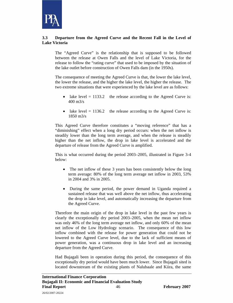
International Finance Corporation Bujagali II: Economic and Financial Evaluation Study Final Report 46 February 2007 26/02/2007-20224
3.3 Departure from the Agreed Curve and the Recent Fall in the Level of Lake Victoria
The “Agreed Curve” is the relationship that is supposed to be followed between the release at Owen Falls and the level of Lake Victoria, for the release to follow the “rating curve” that used to be imposed by the situation of the lake outlet before construction of Owen Falls dam (in the 1950s).
The consequence of meeting the Agreed Curve is that, the lower the lake level, the lower the release, and the higher the lake level, the higher the release. The two extreme situations that were experienced by the lake level are as follows:
• lake level = 1133.2 the release according to the Agreed Curve is: 400 m3/s
• lake level = 1136.2 the release according to the Agreed Curve is: 1850 m3/s
This Agreed Curve therefore constitutes a “moving reference” that has a “diminishing” effect when a long dry period occurs: when the net inflow is steadily lower than the long term average, and when the release is steadily higher than the net inflow, the drop in lake level is accelerated and the departure of release from the Agreed Curve is amplified.
This is what occurred during the period 2003–2005, illustrated in Figure 3-4 below:
• The net inflow of these 3 years has been consistently below the long term average: 80% of the long term average net inflow in 2003, 53% in 2004 and 3% in 2005.
• During the same period, the power demand in Uganda required a sustained release that was well above the net inflow, thus accelerating the drop in lake level, and automatically increasing the departure from the Agreed Curve.
Therefore the main origin of the drop in lake level in the past few years is clearly the exceptionally dry period 2003–2005, when the mean net inflow was only 46% of the long term average net inflow, and only 60% of the mean net inflow of the Low Hydrology scenario. The consequence of this low inflow combined with the release for power generation that could not be lowered to the Agreed Curve level, due to the lack of sufficient means of power generation, was a continuous drop in lake level and an increasing departure from the Agreed Curve.
Had Bujagali been in operation during this period, the consequence of this exceptionally dry period would have been much lower. Since Bujagali sited is located downstream of the existing plants of Nalubaale and Kiira, the same
International Finance Corporation Bujagali II: Economic and Financial Evaluation Study Final Report 47 February 2007 26/02/2007-20224
release will be used a second time at Bujagali and will generate 1.2 times the power already generated by the turbines of Nalubaale – Kiira (the ratio 1.2 is due to the higher head available at Bujagali). Therefore, with Bujagali in operation, the generation of the same total power and energy would require a release of only 45% (1/2.2) from the lake as compared to the present situation without Bujagali.
Figure 3-4: Lake Victoria - Time Series of Outflows and Lake levels - 2000 to 2005 (the right scale applies to lake levels only)
-300-200-100
0100200300400500600700800900
100011001200130014001500
01/01/2000 31/12/2000 31/12/2001 31/12/2002 01/01/2004 31/12/2004 31/12/2005
Date
Out
flow
(m3/
s)
1133.0
1133.5
1134.0
1134.5
1135.0
1135.5
1136.0
Lak
e V
icto
ria
Lev
el (m
)
Q(Agreed Curve) Qactual Departure Lake Levels
3.4 Lake Operation Modelling and Energy Generation Evaluation
Reservoir operation modelling was performed to calculate the firm release and the firm energy generation in each of the hydrology scenarios.
The reservoir operation studies required the comparison of alternative operation rules of Lake Victoria to be made. The main options for the period after commissioning of Bujagali are: i) to return to the strict commitment to the Agreed Curve, and ii) to follow the Agreed Curve but in a broader sense, allowing for a constant release to be applied when the lake level fluctuates within a certain range.
As shown in Appendix B7 and in the figures below, these operation rules do not affect much the minimum and maximum levels reached by the lake during extremely dry or wet periods. The advantage of the second operation rule (Agreed Curve by steps, or “constant release”) is that, during periods of several months or years, the constant release allows for a better planning of additional means of power generation in the country (and in the region, as soon as exchanges of power will be made possible by interconnections).

International Finance Corporation Bujagali II: Economic and Financial Evaluation Study Final Report 48 February 2007 26/02/2007-20224
In the comparison below, the “Constant release” operation consisted in releasing a constant 687 m3/s for the low hydrology scenario, and 1247 m3/s for the high hydrology scenario, both corresponding to a 95% guarantee in time.
Figure 3-5 and Figure 3-6 below illustrate the difference obtained on the lake level fluctuations for each of the operation rules: “constant release” (or “Agreed Curve by steps”) and “Agreed Curve”.
Figure 3-5: Lake Victoria level in the case of the Low Release – Low Hydrology Scenario (reference period: 60 years from 1900 to 1959)
Figure 3-6: Lake Victoria level in the case of the High Release – High Hydrology Scenario (reference period: 40 years from 1960 to 1999)
1 133
1 134
1 135
1 136
1 137
0 10 20 30 40 50 60Year
Lake
Ele
vatio
n
Calculated Level - rule = Constant ReleaseCalculated Level - rule = Agreed CurveMin. Op. Level
²
1 133
1 134
1 135
1 136
1 137
0 5 10 15 20 25 30 35 40Year
Elev
atio
n
Calculated Level - rule = Constant ReleaseCalculated Level - rule = Agreed CurveMin. Op. Level

International Finance Corporation Bujagali II: Economic and Financial Evaluation Study Final Report 49 February 2007 26/02/2007-20224
These curves show that the lake levels remain similar in all cases, except for the High Hydrology scenario (Figure 3-6), after Year 25. The drop of the “Constant Release” curve is the natural result obtained when the release remains constantly high, when the net basin supply is falling. This is effectively the case after Year 25, when the mean net inflow is approximately 1000 m3/s, while the constant release is 1247 m3/s. This also illustrates how the lake level provides a natural and efficient signal that should be used for adapting the operation rule of the lake. In an optimised operation situation, the fall of the lake level to its minimum acceptable value would have been avoided if the constant release had been reduced to a constant intermediate value between 1247 and 687 m3/s (close to 900 m3/s), as soon as the lake level had decreased below approximately El. 1135.0.
Figure 3-7 and Figure 3-8 chart the variations in energy generation (expressed in terms of continuous power) under each of the operation rules. These figures illustrate the much higher variation of generation that would be associated with the “Agreed Curve” operation rule, as compared to the “constant release” (or “Agreed Curve by steps”) operation.
Figure 3-7: Total Energy Production (in MW continuous) of Nalubaale – Kiira and Bujagali (5 units) according to the operating rule - Case of Low Release – Low
Hydrology Scenario (reference period: 60 years from 1900 to 1959)
0
100
200
300
400
500
600
0 10 20 30 40 50 60Year
P (M
W c
ontiu
ous)
Ptotal acc. to constant release
Ptot acc. to Agreed Curve

International Finance Corporation Bujagali II: Economic and Financial Evaluation Study Final Report 50 February 2007 26/02/2007-20224
Figure 3-8: Total Energy Production (in MW continuous) of Nalubaale – Kiira and Bujagali (5 units) according to the operating rule - Case of the High Release – High
Hydrology Scenario (reference period: 40 years from 1960 to 1999)
These charts also illustrate how the “Constant Release” rule better regulates the outflow from the lake, avoiding the very high spillage that the Agreed Curve imposes when the lake level is high: when the lake level is at El. 1135.5, the lake outflow should be 1390 m3/s continuously according to the Agreed Curve. This means the waste of a large volume of water that would be badly needed during the next extreme dry period. This is also illustrated by the fact that the firm energy of the “Constant release” rule is much higher than for the “Agreed Curve” rule, although the mean outflow and mean energy of both operation rules are identical.
Owing to all these advantages, for the purpose of the economic evaluation of Bujagali, the “constant release” (or “Agreed Curve by steps”) rule was adopted to determine the energy generation capability of each of all hydro options on the Nile downstream of Owen Falls.
The results or reservoir operation modelling are summarized in Table 3-1.
0
100
200
300
400
500
600
0 10 20 30 40Year
P (M
W c
ontiu
ous)
Ptotal acc. to constant release
Ptot acc. to Agreed Curve

International Finance Corporation Bujagali II: Economic and Financial Evaluation Study Final Report 51 February 2007 26/02/2007-20224
Table 3-1: Energy generation capability of each hydro power plant (without accounting for the effect of maintenance)
Low Release / Low Hydrology High Release/ High Hydrology
Plants Units Qmax m3/s
Available Capacity
MW
Firm Energy Generation
GWh/yr
Available Capacity
MW
Firm Energy Generation
GWh/yr
Nalubaale - Kiira Units 1 to 15 2300 203 (1) 972 204 (1) 1740
Bujagali HPP Units 1 to 4 992 200 1 198 200 1 715
(candidate) Units 1 to 5 1240 250 1 198 250 2 132
Karuma HPP Units 1 to 3 594 150 1 295 150 1 302
(candidate) Units 1 to 4 792 158 1 360 200 1 722
Units 1 to 5 990 158 1 360 250 2 141
Units 1 to 6 1188 158 1 360 296 2 523 (1) this value may vary depending on the downstream plants and on the optimum operation rule. (2) lines in bold characters indicate the plants considered as base options in the expansion plans
modelling. (3) the energy figures in the table above do not take account of the impact of plant maintenance. (4) Qmax is the flow required to produce the total rated output of the turbine
generators Before being used in the economic evaluation and expansion plan modelling, adjustments to the above figures were made to account for the impact of maintenance periods (see details in Appendix B, and results in Table 7-6). The loss due to maintenance reaches between 2% and 7% of the above energy generation figures.
The recommended operation rule for Lake Victoria adopted for the analysis is as follows:
Low Hydrology scenario, lake level between 1133.5 and 1135.0: the mean release should be kept around a target value 687 m3/s.
High Hydrology scenario, lake level sustained above 1135.0: the mean release should be kept around a target value 1247 m3/s.
For practical day-to-day operation, the operating regime could be divided into a larger number of constant release steps, say three or four without impacting significantly on the total energy generation available from Nalubaale – Kiira, Bujagali and Karuma. A decision to shift from one release step to another could then be taken by a committee representing the various stakeholders involved in the lake operation. However, for the purposes of the detailed analysis of the least cost generation programme, presented in Section 7, the recommended two-step approach has been adopted.

International Finance Corporation Bujagali II: Economic and Financial Evaluation Study Final Report 52 February 2007 26/02/2007-20224
4 Interim Supply Arrangements (2006-2010)
4.1 Existing Short Term Thermal Plant
As discussed in Section 2.1, the demand in Uganda has grown at about 6% per year over the past five years. The load growth, coupled with the drought and the non-availability of new hydro generation resources, have led to more or less continuous load shedding over the period. In order to address the capacity shortage, GoU entered into a contract with Aggreko for 50 MW of firm capacity on a leased basis for a period of three years commencing in May 2005. In 2006, the government concluded a contract with Aggreko for second 50 MW which came into service in October 2006. The Aggreko I and II leased plants, each plant comprising 64 MW packaged high-speed diesel generator units, each of 1 MW capacity, to provide a total firm capacity of 100 MW. The units operate on distillate fuel (AGO – automotive gas oil).
The GoU waived the duty on the fuel used by the Aggreko plants. The cost of generation from the plant from May to December 2005 was 22.7 US¢/kWh, excluding fuel duty. The fuel component is 17.2 US¢/kWh. Fuel duty adds a further 6.8 US¢/kWh.
4.2 Additional Emergency Thermal Plant
A further 50 MW of emergency thermal plant is currently being planned by GoU for installation in the Kampala area. This plant is being evaluated for IDA support and is expected to be in service by August 2007.
The Government is also currently in the process of procuring a 50MW medium-speed plant on a BOT1 basis. The plant is expected to comprise seven medium speed diesel generator units, each of 8 MW net capacity, providing 50 MW firm capacity. The plant will burn heavy fuel (HFO). The plant is expected to be in service in April 2008 and should be located at the Mutundwe site.
4.3 Biomass Projects
There are three sugar factories in Uganda: Kakira Sugar Works Ltd., Sugar Corporation of Uganda (SCOUL) (at Lugazi) and Kinyara Sugar Works Ltd. All three plants generate electricity from bagasse (cane residue) to meet their own factory and irrigation needs. The total installed capacity of the three plants is 7.2 MW.
1 BOT- build, operate and transfer. It is understood that the plant would be transferred to GoU after six years of operation.
International Finance Corporation Bujagali II: Economic and Financial Evaluation Study Final Report 53 February 2007 26/02/2007-20224
The Kakira Sugar Works (Kakira) is engaged on a project to install high pressure boilers and additional power generating plant that will result in a substantial increase in the electricity output. Kakira has signed a power purchase agreement (PPA) with UETCL to supply electricity to the Ugandan grid. The agreement, signed in the mid-2003, covers 6 MW per day during peak hours (6 pm to midnight) at a price of 4.9 US¢/kWh for a period of 15 years. A second agreement, being discussed at present, is understood to include 12 MW per day from 6 am to 6 pm and 6 MW from 6 pm to midnight at a price of 5.6 US¢/kWh for a period of 10 years. The 6 MW from 6 pm to midnight in the second PPA is in addition to the 6 MW covered by the first PPA; thus the total output of the two PPA’s will be 12 MW exported to the grid every day from 6 am to midnight. The power purchase agreements are on a ‘take or pay’ basis. The scheduled commissioning date for the new plant is mid-2007. It has been assumed that the Kakira plant will deliver 34 GWh in 2007 and 75 GWh per year thereafter.
UETCL has also entered into a PPA with the SCOUL sugar estate for the purchase of 3 MW and up to 22 GWh per year. Supply from SCOUL is scheduled to commence in January 2009.
We understand that as yet there are no firm plans for the export of power from the Kinyara Sugar Works.
There is some potential in Uganda for the generation of electricity from wood waste, coffee husks and rice husks, as identified in the ESMAP study2. However, these biomass resources are considered to be too small and spread out to be economically justifiable for large-scale power generation within the timescale of this study.
4.4 Small Hydro Projects
There are two existing small hydro plants, only Kilembe mines (3 MW) currently exports energy to UETCL. The government has recently concluded power purchase agreements (PPAs), or is in the final stages of negotiations with developers, on a number of small hydro projects to be developed pre-2011 on an IPP basis. The principal characteristics of these projects, the dates they are expected to be in service and the expected tariffs are shown in Table 4-1. The tariffs, which are expressed in 2006 prices, correspond to the values that will be in force once Bujagali is in service. Some are fixed whereas other escalate in line with inflation, which is assumed to be 2.5% p.a. in US$ terms.
2 Uganda: Rural Electrification Strategy Study, UNDP/World Bank, ESMAP; Report 221/99

International Finance Corporation Bujagali II: Economic and Financial Evaluation Study Final Report 54 February 2007 26/02/2007-20224
Table 4-1: Existing and Committed Small Hydro Plants
Kilembe Mines Bugoye Waki Buseruka Kikagati Ishasha
Capacity (MW) 3 13 6 9 10 5.5Energy (GWh) 26.3 56.9 26.3 47.3 70.1 24.1Service date existing Jan-2009 Jan-2009 Jan-2009 mid-2008 Jan-2009Tariff (USc/kWh) 2.54 5.8 5.8 13.54 6.75 5.5
escalated escalated escalated fixed fixed fixed
4.5 Fuel Supply Issues
The AGO fuel for the existing leased diesel plants is supplied by pipeline from Mombasa to Eldoret in Kenya and then by road tanker from Eldoret to Kampala. There are on-going negotiations for a concession to extend the fuel pipeline from Eldoret to Kampala. Assuming that these are successful the pipeline could be in service in early-2008. The estimated cost of the pipeline extension project is US$97 million. Once this is completed the costs of fuel supply to Uganda may decrease, although this will depend on the tariff that is finally agreed.
There is currently a capacity constraint on the Kenya pipeline between Nairobi and Eldoret. However, the pipeline company is planning to remove these constraints by the installation of additional pumps at Sinendet which should double the available capacity at Eldoret. This work should be completed by the end of 2006. A further doubling of the capacity at Eldoret is scheduled in December 2007 when the present 6 inch diameter pipe is replaced by an 8 inch diameter pipe. It is understood that there may be a disruption to supply over the period of this changeover, and it is noted that additional pumping capacity will be required on the Mombasa to Nairobi section at this time.
It is estimated that 100 MW of small high speed diesel generators would require approximately 12,000 m3 of liquid fuel per month, equivalent to approximately 400 m3 per day, or about 10 road tankers per day. As previously noted, the pipeline is used for the transportation of a range of different fuels. At the current capacity of the pipeline to Eldoret, however, the 100 MW of emergency generation would utilise 7% of the available capacity of the pipeline. If it is assumed that AGO is currently pumped for only 20% of the time, this represents a significant change to the proposed pumping regime. It might not be possible to resource this additional fuel requirement from Eldoret until the capacity of the pipeline from Nairobi is increased, and the fuel might therefore need to be trucked by road from Nairobi.
Heavy fuel oil (HFO) is not transported through the pipeline and therefore thermal generation options using HFO would either have to be transported by road all the way from Mombasa, or by rail. In view of the quantities of fuel that would be required and the additional heavy traffic burden this would
International Finance Corporation Bujagali II: Economic and Financial Evaluation Study Final Report 55 February 2007 26/02/2007-20224
impose on the roads, in particular the road between Mombasa and Nairobi, this would have to be cleared first with the Kenyan authorities. The transport of HFO by road all the way from Mombasa would require a substantial investment in new tankers and storage capacity in Kampala. For this reason HFO was not considered a feasible option for the additional 100 MW of short term thermal plant. However, for the medium term, delivery by road might be a feasible option. Alternative transport routes through Tanzania and across Lake Victoria could be options but they are likely to be of the same order of cost as the road option from Mombasa.
The present capacity of Uganda railways to transport large quantities of fuel originating in Mombasa is limited due to the condition of the track and the rolling stock. Uganda railways has only about 100 serviceable tanker wagons at the present time. The railways are also currently in the process of being privatised and therefore their future is somewhat uncertain. However, for the purposes of our analysis of medium/long term thermal options it is assumed that there would be investment made in the railways to make the transport of HFO from Mombasa feasible by mid-2008. We were unable to obtain information on the likely rail transport cost from Mombasa to Kampala from Uganda railways. For the purposes of the present analysis the cost of HFO is based on transport by road from Mombasa to Kampala.
In view of the long transport routes and the possibility of supply disruptions it is considered that fuel storage capacity equivalent to a minimum of 30 days of full-load operation of the thermal plant should be provided in Uganda. For a 100 MW plant burning HFO, about 10,000 m3 of storage tanks would be required. This storage could be provided either by the fuel distributor or the owner/operator of the power plant. The preferred option would be for the plant owner to provide the storage as this would give more flexibility in sourcing the fuel.
4.6 Fuel Types and Costs
As discussed in the previous section, the existing diesel plant in Kampala uses automotive diesel oil (ADO). Heavy fuel oil (HFO) which is a medium fuel oil (180 cSt) that can be pumped without heating is also used in Uganda, primary by the cement industry, but also in a small diesel plant in the north-west of the country. HFO is supplied either by rail or by road from Mombasa. Both these products are generally sourced from the Middle East. The third liquid fuel considered for thermal plant in Uganda is industrial diesel oil (IDO). This fuel is slightly heavier than AGO and can be used for industrial gas turbines.
The fuel costs use for the study are based on the latest World Bank crude oil price forecast for the period to 2015, shown in Table 4-2. Post-2015 prices are assumed to remain constant at the 2015 levels, expressed in constant 2006 US$ terms.
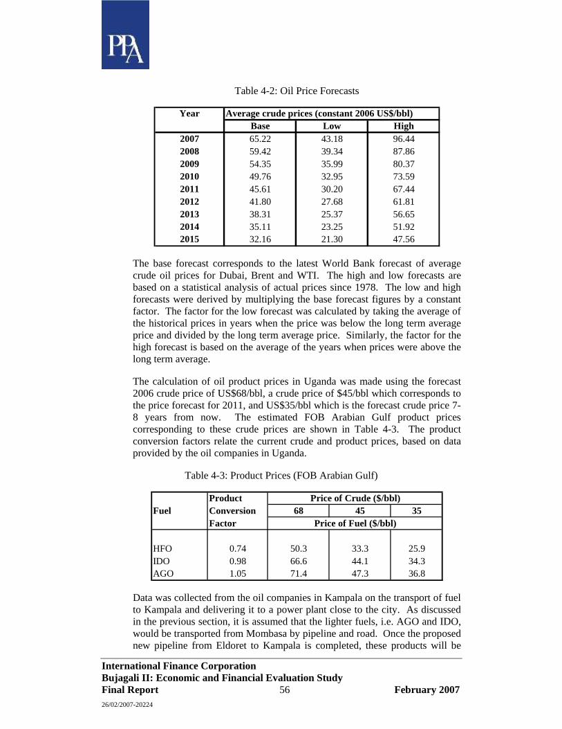
International Finance Corporation Bujagali II: Economic and Financial Evaluation Study Final Report 56 February 2007 26/02/2007-20224
Table 4-2: Oil Price Forecasts
YearBase Low High
2007 65.22 43.18 96.442008 59.42 39.34 87.862009 54.35 35.99 80.372010 49.76 32.95 73.592011 45.61 30.20 67.442012 41.80 27.68 61.812013 38.31 25.37 56.652014 35.11 23.25 51.922015 32.16 21.30 47.56
Average crude prices (constant 2006 US$/bbl)
The base forecast corresponds to the latest World Bank forecast of average crude oil prices for Dubai, Brent and WTI. The high and low forecasts are based on a statistical analysis of actual prices since 1978. The low and high forecasts were derived by multiplying the base forecast figures by a constant factor. The factor for the low forecast was calculated by taking the average of the historical prices in years when the price was below the long term average price and divided by the long term average price. Similarly, the factor for the high forecast is based on the average of the years when prices were above the long term average.
The calculation of oil product prices in Uganda was made using the forecast 2006 crude price of US$68/bbl, a crude price of $45/bbl which corresponds to the price forecast for 2011, and US$35/bbl which is the forecast crude price 7-8 years from now. The estimated FOB Arabian Gulf product prices corresponding to these crude prices are shown in Table 4-3. The product conversion factors relate the current crude and product prices, based on data provided by the oil companies in Uganda.
Table 4-3: Product Prices (FOB Arabian Gulf)
ProductFuel Conversion 68 45 35
Factor
HFO 0.74 50.3 33.3 25.9IDO 0.98 66.6 44.1 34.3AGO 1.05 71.4 47.3 36.8
Price of Fuel ($/bbl)
Price of Crude ($/bbl)
Data was collected from the oil companies in Kampala on the transport of fuel to Kampala and delivering it to a power plant close to the city. As discussed in the previous section, it is assumed that the lighter fuels, i.e. AGO and IDO, would be transported from Mombasa by pipeline and road. Once the proposed new pipeline from Eldoret to Kampala is completed, these products will be

International Finance Corporation Bujagali II: Economic and Financial Evaluation Study Final Report 57 February 2007 26/02/2007-20224
transported by pipeline all the way from Mombasa. It is assumed that the transport cost through the new pipeline will be similar to the current road transport cost between Eldoret and Kampala. The HFO will not be transported through the pipeline and therefore it has to come either by road from Mombasa or by rail. The road cost is currently US$ 110/tonne and following discussions with the oil companies this has been used for both road and rail transport. In principle rail should be less expensive but it was felt that the railways are in need of major refurbishment and therefore the rail costs will not be much different over the period of this study. Details of the shipping, transport and other costs are shown in Table 4-4. The ‘Other’ costs include inspection, port and storage fees in Kenya and Kampala, and the oil company margin.
Table 4-4: Fuel Shipping, Transport and Handling Costs
Item Light Fuels Heavy FuelsUS$/tonne US$/tonne
Shipping to Mombasa 55.0 55.0Pipeline 40.0Road/rail 60.0 110.0Other * 93.0 65.0Total 248.0 230.0* includes company margin and local storage charges.
The assumed specific gravity and heating values of the fuels are shown in Table 4-5. The heating values are net (LHV) figures.
Table 4-5: Fuel Gravity and Heating Values
Fuel Densitybbl/tonne GJ/bbl GJ/tonne
HFO 6.5 6.27 40.8IDO 7.3 5.80 42.36AGO 7.5 5.65 42.40* based on LHV
Heat content*
The costs of the various fuels delivered to Kampala are shown in Table 4-6 in both US$/tonne and US$/GJ.
Table 4-6: Fuel Prices Delivered to Kampala
Crude price (US$/bbl)Fuel US$/te US$/GJ US$/te US$/GJ US$/te US$/GJHFO 557.1 13.65 446.5 10.94 398.4 9.76IDO 721.5 17.02 556.9 13.14 485.4 11.45AGO 768.4 18.13 587.2 13.86 508.5 12.00
3568 45

International Finance Corporation Bujagali II: Economic and Financial Evaluation Study Final Report 58 February 2007 26/02/2007-20224
4.7 Interim Generating Plant
The ToR for the study require the Consultant to consider the generating capacity position during the interim period until 2011 when Bujagali is expected to be commissioned. Since the Interim Report was submitted, GoU has progressed its plans for the supply of electricity during this interim period. As discussed in the preceding sections, the government is intending to lease a further 100 MW of emergency diesel plant and has planned for a 50 MW diesel IPP burning HFO. These plants, together with the proposed small hydro and biomass-fired developments will supplement the output of the existing hydro plants at Nalubaale and Kiira. The extent to which the existing and proposed interim plant will be able to meet the forecast demand in Uganda will depend on the rainfall patterns in the region and the hydrology of Lake Victoria. A study was commissioned by the World Bank in March 2006 to examine the electricity supply arrangements during the interim period up to the end of 2010. The study was subsequently revised in October 2006 to take account of the most recent data and developments in the procurement of additional generating capacity. A summary of the interim supply arrangements, as envisaged at the time of writing this report, is presented in Table 4-7.

International Finance Corporation Bujagali II: Economic and Financial Evaluation Study Final Report 59 February 2007 26/02/2007-20224
Table 4-7: Interim Generation Expansion Plan, 2006-2010
Firm Capacity
(MW)
Fuel Commissioning Retirement
Thermal:
Aggreko I lease (existing)
Aggreko II lease (contracted)
IDA lease (not yet contracted)
IPP (BOT)
50
50
50
50
AGO
AGO
AGO
HFO
May 2005
Oct 2006
Aug 2007
Apr 2008
Mar 20081
Dec 20082
Dec 2010
BOT3
Mini-hydro:
Bugoye
Waki
Buseruka
Kikagati
Ishasha
13
6
9
10
5.5
Jan 2009
Jan 2009
Jan 2009
Jul 2008
Jan 2009
Cogeneration/biomass:
Kakira Sugar
Sugar Corporation (SCOUL)
12
3
Jul 2007
Jan 2009
1 The termination date will coincide with the commissioning of the HFO diesel plant. 2 Contract may be extended as necessary. 3 To be transferred after six years’ operation. Source: World Bank
4.8 Electricity Imports
The only feasible potential source of imports in the short/medium term up to the commissioning of Bujagali is from Kenya. Discussions were held with the Kenyan Ministry of Energy and KPLC, both of whom indicated that Kenya is also suffering similar problems to Uganda caused by the regional drought leading to shortages of generating capacity and is therefore unlikely to have any significant surplus electricity for export to Uganda. Since the discussions were held with the Kenyans, UETCL has negotiated a contract for the import of 20 MW during off-peak periods. It is understood that this contract will only remain in force until 2011 when Bujagali is expected to be commissioned.
4.9 Plant Existing in 2011
The plant that should remain operational from 2011 when Bujagali is due to come into service comprises a mix of hydro, biomass and conventional

International Finance Corporation Bujagali II: Economic and Financial Evaluation Study Final Report 60 February 2007 26/02/2007-20224
thermal plants with an aggregate capacity of 474.5 MW, as shown in Table 4-8. The available capacity of Nalubaale – Kiira is generally significantly lower than the installed capacity, as discussed in Section 5.3, Table 5-2.
Table 4-8: Generating Capacity Expected to be in Service in 2011
Installed Capacity
(MW)
Hydro:
Nalubaale – Kiira
Bugoye
Waki
Buseruka
Kikagati
Ishasha
380
13
6
9
10
5.5
Thermal:
IPP (BOT)
50
Cogeneration/biomass:
Kakira Sugar
Sugar Corporation (SCOUL)
12
3
Total 474.5

International Finance Corporation Bujagali II: Economic and Financial Evaluation Study Final Report 61 February 2007 26/02/2007-20224
5 Candidate Plant (2011-2020)
5.1 Conventional Thermal Plant
Since Uganda has no indigenous fossil fuel reserves that are currently developed, all fuel for conventional thermal plant will have to be imported. The conventional thermal options considered for Uganda are:
• Medium and low speed diesels burning HFO, (180 cSt.)3 with unit sizes of 10 MW to 50 MW net;
• Open cycle aero-derivative gas turbines with unit sizes of 30 MW ISO rating (26 MW site rating) burning AGO, or industrial gas turbines with a capacity 67 MW ISO rating (57 MW site rating).
• Combined cycle gas turbine plant, burning either IDO with a unit size of 100 MW ISO rating (84 MW site rating); and
• Steam plant burning HFO with a unit size of 100 MW net. Coal-fired steam plant was not considered in view of the non-availability of coal in Uganda, the high shipping and rail haulage costs and the higher capital cost of this type of plant as compared to steam or diesel plant burning HFO.
• Geothermal plant with a unit size of 40MW.
Cost and performance data for the candidate thermal plants, split between fixed and variable elements, are summarised in Table 5-1. The costs are based on prices prevailing in January 2006. The fuel costs shown in the table are based on the 2006 oil price of US$ 68/bbl.
No site identification or other studies have been carried out for the potential thermal plant candidates; for the purposes of this analysis it has been assumed that the plants would be sited close to Kampala. The costs of the thermal plants therefore exclude the costs of connection to the grid but do include for the cost of the switchyard. The cost estimates are assumed to include for on-site fuel storage.
Similarly, there is no allowance for off-site fuel delivery and storage as this is assumed to be included in the fuel prices.
3 180cSt fuel oil is available in the region; the oil does not require heating to allow it to be handled, as would be required for heavier fuel oils.
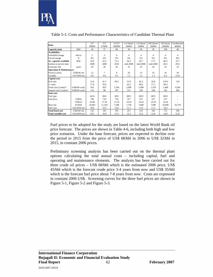
International Finance Corporation Bujagali II: Economic and Financial Evaluation Study Final Report 62 February 2007 26/02/2007-20224
Table 5-1: Costs and Performance Characteristics of Candidate Thermal Plant
Item:GT
30MWGT
67MWCCGT
100MWLS Diesel
30MWLS Diesel
50MWMS Diesel
20MWOil Steam 100MW
Geothermal 40MW
Capacity (net) MW 26 57 84 30 50 20 100 40Availability:Scheduled outage wks/yr 2 2 4 4 4 4 4 4Forced outage % 4% 4% 5% 5% 5% 5% 6% 8%Av. capacity available MW 24.0 52.5 73.3 26.2 43.7 17.5 86.3 33.7Earliest in-service date 2008 2008 2010 mid-2008 mid-2008 mid-2008 2011 2011Economic life years 20 20 20 25 25 20 25 25Operation & Maintenance:Fixed (2 units) US$/kW net 12 7 8 20 13 35 10 50Variable USc/kWh net 0.6 0.6 0.5 1.2 1.2 1.3 0.5 0.25Capital cost:First unit 21.6 41.7 99.2 51.8 82.3 20.8 119.0 1342+ units 17.8 35.6 - 43.2 68.6 17.3 90.4 -Total cost (2 units)* US$/kW avail. 933 833 1,594 2,096 1,998 1,259 1,468 4,504Annual cost (2 units)* US$/kW avail. 110 98 187 231 220 148 162 496Fuel cost:Fuel type AGO IDO IDO HFO HFO HFO HFO -Fuel price US$/te 784 734 734 557 557 557 557 -
US$/GJ 18.48 17.34 17.34 14.34 14.34 14.34 14.34 -Heat rate kJ/kWh 10,065 11,105 7,390 7,730 7,680 7,990 10,000 25,270Fuel cost: USc/kWh net 18.6 19.3 12.8 11.1 11.0 11.5 14.3 -Total fixed cost US$/kW net 122 105 195 251 233 183 172 546Total variable cost USc/kWh net 19.2 19.9 13.3 12.3 12.2 12.8 14.8 0.25
Fuel prices to be adopted for the study are based on the latest World Bank oil price forecast. The prices are shown in Table 4-6, including both high and low price scenarios. Under the base forecast, prices are expected to decline over the period to 2015 from the price of US$ 68/bbl in 2006 to US$ 32/bbl in 2015, in constant 2006 prices.
Preliminary screening analysis has been carried out on the thermal plant options calculating the total annual costs – including capital, fuel and operating and maintenance elements. The analysis has been carried out for three crude oil prices – US$ 68/bbl which is the estimated 2006 price, US$ 45/bbl which is the forecast crude price 3-4 years from now and US$ 35/bbl which is the forecast fuel price about 7-8 years from now. Costs are expressed in constant 2006 US$. Screening curves for the three fuel prices are shown in Figure 5-1, Figure 5-2 and Figure 5-3.
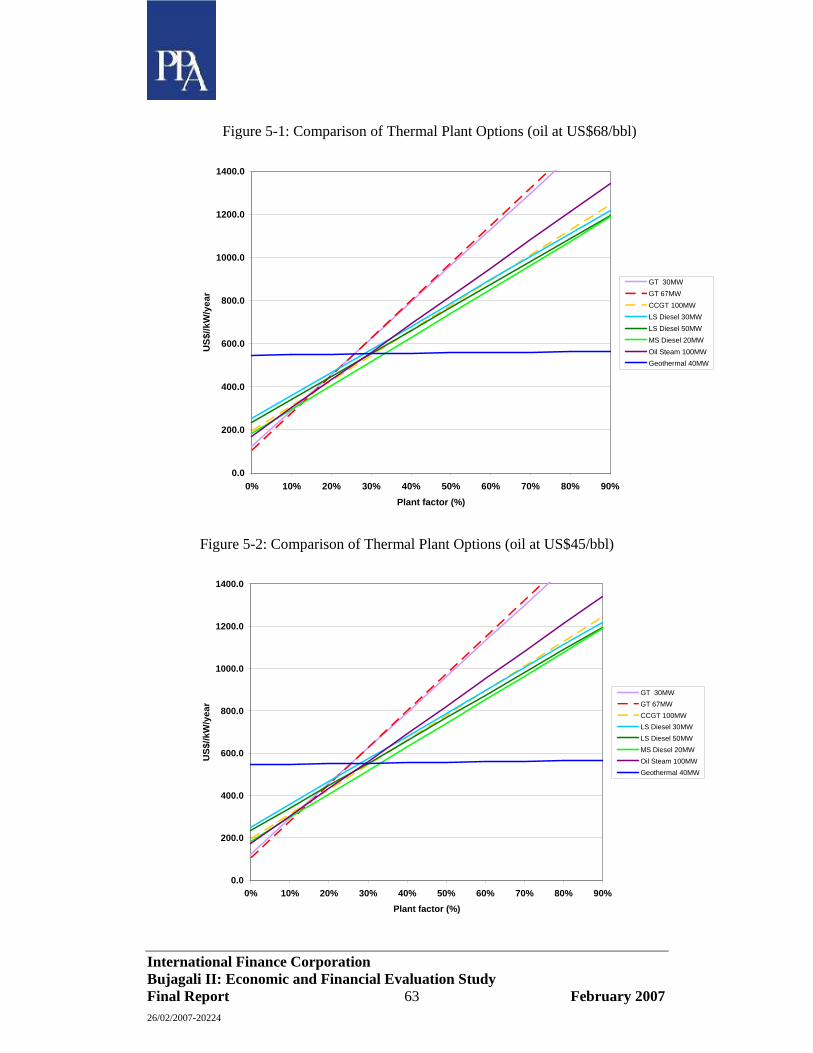
International Finance Corporation Bujagali II: Economic and Financial Evaluation Study Final Report 63 February 2007 26/02/2007-20224
Figure 5-1: Comparison of Thermal Plant Options (oil at US$68/bbl)
0.0
200.0
400.0
600.0
800.0
1000.0
1200.0
1400.0
0% 10% 20% 30% 40% 50% 60% 70% 80% 90%Plant factor (%)
US$
//kW
/yea
r
GT 30MWGT 67MWCCGT 100MWLS Diesel 30MWLS Diesel 50MWMS Diesel 20MWOil Steam 100MWGeothermal 40MW
Figure 5-2: Comparison of Thermal Plant Options (oil at US$45/bbl)
0.0
200.0
400.0
600.0
800.0
1000.0
1200.0
1400.0
0% 10% 20% 30% 40% 50% 60% 70% 80% 90%Plant factor (%)
US$
//kW
/yea
r
GT 30MWGT 67MWCCGT 100MWLS Diesel 30MWLS Diesel 50MWMS Diesel 20MWOil Steam 100MWGeothermal 40MW
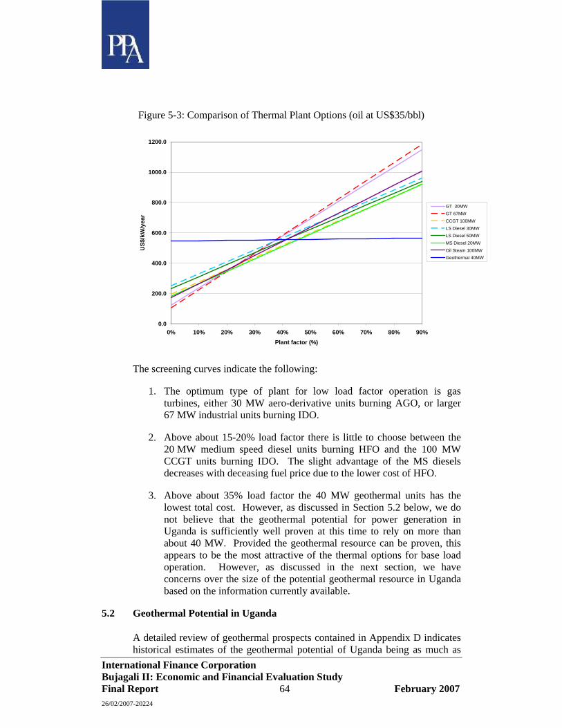
International Finance Corporation Bujagali II: Economic and Financial Evaluation Study Final Report 64 February 2007 26/02/2007-20224
Figure 5-3: Comparison of Thermal Plant Options (oil at US$35/bbl)
0.0
200.0
400.0
600.0
800.0
1000.0
1200.0
0% 10% 20% 30% 40% 50% 60% 70% 80% 90%Plant factor (%)
US$
/kW
/yea
r
GT 30MWGT 67MWCCGT 100MWLS Diesel 30MWLS Diesel 50MWMS Diesel 20MWOil Steam 100MWGeothermal 40MW
The screening curves indicate the following:
1. The optimum type of plant for low load factor operation is gas turbines, either 30 MW aero-derivative units burning AGO, or larger 67 MW industrial units burning IDO.
2. Above about 15-20% load factor there is little to choose between the 20 MW medium speed diesel units burning HFO and the 100 MW CCGT units burning IDO. The slight advantage of the MS diesels decreases with deceasing fuel price due to the lower cost of HFO.
3. Above about 35% load factor the 40 MW geothermal units has the lowest total cost. However, as discussed in Section 5.2 below, we do not believe that the geothermal potential for power generation in Uganda is sufficiently well proven at this time to rely on more than about 40 MW. Provided the geothermal resource can be proven, this appears to be the most attractive of the thermal options for base load operation. However, as discussed in the next section, we have concerns over the size of the potential geothermal resource in Uganda based on the information currently available.
5.2 Geothermal Potential in Uganda
A detailed review of geothermal prospects contained in Appendix D indicates historical estimates of the geothermal potential of Uganda being as much as

International Finance Corporation Bujagali II: Economic and Financial Evaluation Study Final Report 65 February 2007 26/02/2007-20224
450MWe are substantially over-stated. The true potential is likely to be in the order of only 10% of this figure. The key findings of the review of geothermal Uganda review are summarised in the following paragraphs.
There are three principal geothermal resource areas in Uganda. Two of these, at Katwe and Buranga, are interpreted in the assessment carried out for this report to be low grade resources with reservoir temperatures of only some 100ºC and consequently with nil potential for commercial scale power generation. The third prospect, at Kibiro, is more promising and appears to be a medium grade geothermal resource with reservoir temperatures of about 220ºC. Kibiro is therefore considered to be the only geothermal resource in Uganda with clear potential for power development.
The size of a geothermal power plant that could be developed at Kibiro will depend on actual resource conditions that have yet to be proven by exploration drilling. Nonetheless, deep geothermal resource conditions can be inferred from the results of surface exploration surveys undertaken to date. By this means it is assessed that the Kibiro resource may prove to be suitable for the future development of either a 20MWe condensing steam power plant or a 40MWe organic Rankin cycle binary plant, both with an operational life of at least 25 years.
The cost of developing a 40 MWe binary cycle geothermal power plant at Kibiro is assessed at US$ 134 million which equates to a cost of US$ 3350 per kWe installed. This cost includes all items for a full “greenfield” development, including project infrastructure, wells, steam field, power plant, transformers and transmission facilities.
A preliminary project schedule programme for a 40MWe binary cycle development at Kibiro has been developed based on the following assumptions:
• Pre feasibility work will be completed during the first half of 2006 and funding in the amount of US$ 9.0 million would need to be sought for the drilling of a two well exploration programme at Kibiro;
• Preparation of the project for drilling would commence in early 2007 after funding has been obtained;
• Exploration drilling, well testing and resource evaluation would be undertaken from late 2007 to mid 2008 culminating in the preparation of a detailed, “bankable” feasibility study for the project;
• Funding would be sought for a 40MWe power plant development, in the amount of about US$ 120 million. It is expected that this could be obtained by end of the first quarter 2009;
International Finance Corporation Bujagali II: Economic and Financial Evaluation Study Final Report 66 February 2007 26/02/2007-20224
• Production drilling would commence in early 2009 with requirements assessed at 7 production wells and 5 re-injection wells. This would require one drilling rig to be working continuously for 24 months through the end of the first quarter of 2011;
• In parallel with this production drilling, EPC contracts for both the geothermal steam field and the power plant would be prepared and let;
• Power plant construction activities would be undertaken between early 2009 and early 2011; and
• Plant commissioning would commence in the second quarter of 2011 and commercial operation of the 40MWe plant in mid-2011.
The overall programme to undertake the exploration drilling, production drilling and steam field and power plant construction would thus require a total of approximately 52 months from the time that the exploration drilling programme is commenced.
5.3 Existing Hydro
The hydro power plants presently connected to the grid are essentially the Nalubaale and Kiira power plants, located at the outlet of Lake Victoria.
In addition to these two plants, which generate most of the energy consumed in the Uganda power system, some small hydro power plants exist, such as Kikagati, Maziba, Kisisi or Mobuku. Nevertheless, most of these plants either supply power to local consumption centres, not connected to the main grid, or represent a very minor part of the total power production of the system. Therefore their influence on the economic evaluation of Bujagali HPP is negligible, and it was found unnecessary to include them in the modelling of the whole power system.
Nalubaale HPP
Nalubaale hydro power plant was commissioned in 1954, under the name of Owen Falls. It is located near Jinja, at the source of the White Nile, a few kilometres downstream of the outlet of Lake Victoria. The plant is made of:
• a concrete gravity dam,
• a powerhouse presently housing 10 units of 18 MW capacity, after the rehabilitation and upgrading (from 15 MW) implemented from 1989 to 1998, thus with a total capacity of 180 MW.
Before construction of this dam and powerhouse, the outflow from Lake Victoria used to be controlled by the natural section of Rippon Falls, located between Owen Falls and Lake Victoria. It is now entirely controlled by the dam and the outlets of both Nalubaale and Kiira plants, except for lower lake

International Finance Corporation Bujagali II: Economic and Financial Evaluation Study Final Report 67 February 2007 26/02/2007-20224
levels for which the head losses in the river upstream of the dam could increase to such an extent that this upstream river section would regain the hydraulic control of the flow. This is exhaustively shown in the reports of the "Study on Water management of Lake Victoria" performed by WREM in 2004 – 2005.
As a result of the development of alkali-silica reaction between components of the concrete, both the dam and the powerhouse structure show serious deteriorations, with the most serious signs visible in the powerhouse. The concrete expansion, caused by this chemical reaction, has major consequences not only on the integrity of the structure itself, but also on the smooth operation of the equipment supported by the concrete structure. This required various remedial works to be made on the structure itself (e.g. tensioned anchors) and on the equipment that will need to be repeated in the future. Proper monitoring of the structures also needs to be more thoroughly and frequently applied that in other plants without this kind of pathology.
According to the latest Annual Inspection Reports (Year 2005) prepared by Lahmeyer International, there is no present risk in the condition and stability of the main dam, but the situation is quite alarming for the intake structure, the headrace bridge and the powerhouse structure. The analysis of monitoring instrument records and visual inspection of the works leads to the conclusion that "a long term safe operation of the turbines cannot be guaranteed".
Despite these exceptional circumstances, the monitoring system installed in the structures is found by Lahmeyer insufficient to properly assess the evolution of the situation and to constitute a real surveillance tool for the operator of the plants, between two annual inspections. This increases the risk of unforeseen outage of Nalubaale plant. On the other hand, in the case when the operation of part or all of the units at Nalubaale plant would need to be stopped for a long period of time, for a major structural repair or retrofit, the five units of Kiira are able to deliver about the same power as at Nalubaale, with commissioning of Units 14 and 15 (completed in March 2006), with a maximum turbine flow of approximately 1 160 m3/s.
The main characteristics of the plants at the Owen Falls complex are summarised in Table 5-2.

International Finance Corporation Bujagali II: Economic and Financial Evaluation Study Final Report 68 February 2007 26/02/2007-20224
Table 5-2: Main characteristics of Nalubaale and Kiira hydro power plants
Item Nalubaale Kiira (4 River, location Victoria Nile (approx. 7 km
downstream of the outlet of Lake Victoria, near Jinja), left bank
Victoria Nile (approx. 7 km downstream of the outlet of Lake Victoria, near Jinja), right bank
Date of commissioning 1954 (first two units) to 1968 (last of 10 units)
1989-98: upgrading to 18 MW
2000 (Units 11, 12) 2002 (Unit 13) March 2006 (Units 14, 15)
Hydrology: - Mean flow 1900 – 1960 - Mean flow 1961 – 2005 - Mean flow 1900 – 2005
662 m3/s
1 143 m3/s 866 m3/s
662 m3/s
1 143 m3/s 866 m3/s s
HEM Equipment - Total installed capacity - Turbine design flow
- 10 x 18 = 180 MW - 10 x 110 = 1 100 m3/s
- 5 x 40 = 200 MW - 5 x 232 = 1 160 m3/s
Energy generation capability: - Base hydrology (1900-1960) - High hydrology (1961-2000)
972 GW/year
1740 GWh/year
5.4 Bujagali HPP
5.4.1 Characteristics of the project
Bujagali HPP has been designed at feasibility stage in 1998–1999, by Knight Pisesold – Merz and McLellan, for the first developer of the project, AES Nile Power. After the withdrawal of AES from the project, the GoU has undertaken to develop the project under a new Public – Private Participation arrangement.
Since the feasibility study of 1998–1999, the design of the project has been slightly modified, although the location of the works and general arrangement remain substantially identical:
• location of the works at Dumbell Island, which takes advantage of the island to minimize the volume and cost of the dam, and to minimize the cost of river control during construction;
• embankment dam on the right bank, and powerhouse on the left bank channel;
4 After commissioning of Units 14 and 15, scheduled in March 2006
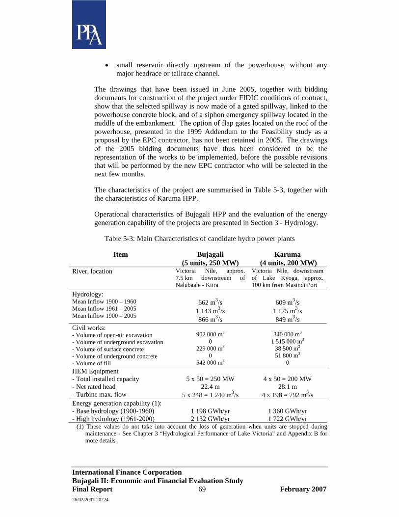
International Finance Corporation Bujagali II: Economic and Financial Evaluation Study Final Report 69 February 2007 26/02/2007-20224
• small reservoir directly upstream of the powerhouse, without any major headrace or tailrace channel.
The drawings that have been issued in June 2005, together with bidding documents for construction of the project under FIDIC conditions of contract, show that the selected spillway is now made of a gated spillway, linked to the powerhouse concrete block, and of a siphon emergency spillway located in the middle of the embankment. The option of flap gates located on the roof of the powerhouse, presented in the 1999 Addendum to the Feasibility study as a proposal by the EPC contractor, has not been retained in 2005. The drawings of the 2005 bidding documents have thus been considered to be the representation of the works to be implemented, before the possible revisions that will be performed by the new EPC contractor who will be selected in the next few months.
The characteristics of the project are summarised in Table 5-3, together with the characteristics of Karuma HPP.
Operational characteristics of Bujagali HPP and the evaluation of the energy generation capability of the projects are presented in Section 3 - Hydrology.
Table 5-3: Main Characteristics of candidate hydro power plants
Item Bujagali (5 units, 250 MW)
Karuma (4 units, 200 MW)
River, location Victoria Nile, approx. 7.5 km downstream of Nalubaale - Kiira
Victoria Nile, downstream of Lake Kyoga, approx. 100 km from Masindi Port
Hydrology: Mean Inflow 1900 – 1960 Mean Inflow 1961 – 2005 Mean Inflow 1900 – 2005
662 m3/s
1 143 m3/s 866 m3/s
609 m3/s
1 175 m3/s 849 m3/s
Civil works: - Volume of open-air excavation - Volume of underground excavation - Volume of surface concrete - Volume of underground concrete - Volume of fill
902 000 m3
0 229 000 m3
0 542 000 m3
340 000 m3
1 515 000 m3
38 500 m3 51 800 m3
0 HEM Equipment - Total installed capacity - Net rated head - Turbine max. flow
5 x 50 = 250 MW
22.4 m 5 x 248 = 1 240 m3/s
4 x 50 = 200 MW
28.1 m 4 x 198 = 792 m3/s
Energy generation capability (1): - Base hydrology (1900-1960) - High hydrology (1961-2000)
1 198 GWh/yr 2 132 GWh/yr
1 360 GWh/yr 1 722 GWh/yr
(1) These values do not take into account the loss of generation when units are stopped during maintenance - See Chapter 3 “Hydrological Performance of Lake Victoria” and Appendix B for more details

International Finance Corporation Bujagali II: Economic and Financial Evaluation Study Final Report 70 February 2007 26/02/2007-20224
5.4.2 Construction Costs
The economic cost of construction of Bujagali HPP has been evaluated on the basis of the following data and assumptions:
• design drawings and volume of the works presented in the bidding documents of June 2005, and more recent information provided by the Developer on the bidding process of the EPC contract;
• Feasibility study of 1998 and its addendum of 1999;
• Unit rates of civil works and power plant equipment obtained from international bidding on similar works, taking into account the recent trend of tightening of the market in the hydro power sector and a substantial increase in the price of some construction material;
• The results of the EPC contract negotiations reached by 31 January 2007;
• All costs are expressed in US$, January 2006 values. They do not include any tax or provision for escalation of costs.
The volumes of work presented in the June 2005 bidding documents have been aggregated into a reduced number of items, for evaluation purposes. The aggregated volumes of work have been checked for the main items such as volume of the dam, excavations, etc., and they have been found in fairly good agreement with the volumes in the Bill of Quantity of June 2005.
Costs are presented for Bujagali equipped in a single stage with five units of 50 MW each, and for a similar project equipped with four units of 50 MW each.
The resulting construction costs are presented in Table 5-4 and Table 5-5, together with the total implementation cost5.
The transmission costs for Bujagali are based on the design proposed by the consultants appointed by the project sponsors. The design includes for a double circuit 132 kV transmission line between Bujagali and Kawanda
5 Just after this report was completed, BEL informed PPA and the Bank Group of the most recent results of on-going negotiations with the EPC contractor, indicating the addition of a $20 to $ 30 million risk premium in exchange for a comprehensive turnkey contract, plus another $ 5 to $10 million for improvements to the electro-mechanical works, bringing the total EPC cost increase into a range of $30 to $35 millions, nominal and undiscounted. At the same time, BEL and the contractor are negotiating an incentive scheme to accelerate commissioning by 3 to 4 months, which would create for Uganda a real economic cost saving on thermal plant operation estimated at $30 to $40 million (in dollars of 2006). The net impact of these proposed changes on the project’s economic viability is judged to be minimal.

International Finance Corporation Bujagali II: Economic and Financial Evaluation Study Final Report 71 February 2007 26/02/2007-20224
substation, near Kampala, plus a further transmission link between Kawanda and Mutundwe in Kampala. The Bujagali substation will be tied into the existing 132 kV line between Jinja and Torroro. The costs of the transmission are based on the estimates proposed by the sponsor’s consultants. The Bujagali – Kawanda line is to be designed to be suitable for future uprating to 220 kV.
5.4.3 Other costs and resulting total cost of implementation
In addition to direct construction costs, other costs include:
• the costs of all engineering activities, evaluated in the context of an EPC contract, including the cost of an Independent Consultant to guarantee the quality of the design and construction work of the EPC contractor.
• environmental and social impact costs, have been updated in the light of the work being carried out by Burnside for the project sponsor. The incremental environmental costs adopted are based on this information and the work carried our by the consultant’s E&S specialists. The build-up of the E&S costs is presented in Section 6. The E&S costs have been reviewed and updated since the submission of the Draft Final Report, based on the Final ESIA Report by Burnside, the sponsor’s consultants which only became available too late to be considered in the Draft Final Report.
• other development costs linked to financing fees, developer's fees, etc.
The Bujagali cost estimates shown in Table 5-4 and Table 5-5 exclude interest during construction (IDC). It should be noted that IDC is accounted for in the economic analysis through the phasing of the construction costs with IDC at 10% per annum.
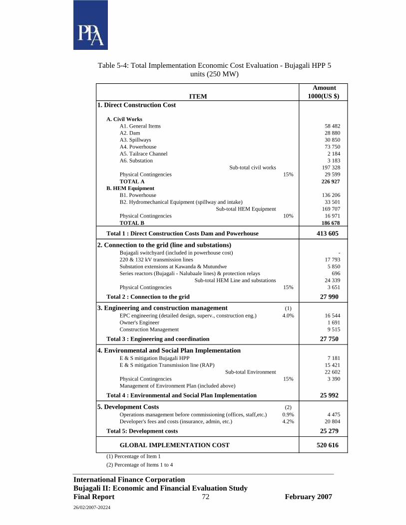
International Finance Corporation Bujagali II: Economic and Financial Evaluation Study Final Report 72 February 2007 26/02/2007-20224
Table 5-4: Total Implementation Economic Cost Evaluation - Bujagali HPP 5 units (250 MW)
ITEM Amount
1000(US $) 1. Direct Construction Cost
A. Civil WorksA1. General Items 58 482 A2. Dam 28 880 A3. Spillways 30 850 A4. Powerhouse 73 750 A5. Tailrace Channel 2 184 A6. Substation 3 183
Sub-total civil works 197 328 Physical Contingencies 15% 29 599 TOTAL A 226 927
B. HEM EquipmentB1. Powerhouse 136 206 B2. Hydromechanical Equipment (spillway and intake) 33 501
Sub-total HEM Equipment 169 707 Physical Contingencies 10% 16 971 TOTAL B 186 678
Total 1 : Direct Construction Costs Dam and Powerhouse 413 605
2. Connection to the grid (line and substations)Bujagali switchyard (included in powerhouse cost) - 220 & 132 kV transmission lines 17 793 Substation extensions at Kawanda & Mutundwe 5 850 Series reactors (Bujagali - Nalubaale lines) & protection relays 696
Sub-total HEM Line and substations 24 339 Physical Contingencies 15% 3 651
Total 2 : Connection to the grid 27 990
3. Engineering and construction management (1)EPC engineering (detailed design, superv., construction eng.) 4.0% 16 544 Owner's Engineer 1 691 Construction Management 9 515
Total 3 : Engineering and coordination 27 750
4. Environmental and Social Plan ImplementationE & S mitigation Bujagali HPP 7 181 E & S mitigation Transmission line (RAP) 15 421
Sub-total Environment 22 602 Physical Contingencies 15% 3 390 Management of Environment Plan (included above)
Total 4 : Environmental and Social Plan Implementation 25 992
5. Development Costs (2)Operations management before commissioning (offices, staff,etc.) 0.9% 4 475 Developer's fees and costs (insurance, admin, etc.) 4.2% 20 804
Total 5: Development costs 25 279
GLOBAL IMPLEMENTATION COST 520 616 (1) Percentage of Item 1(2) Percentage of Items 1 to 4
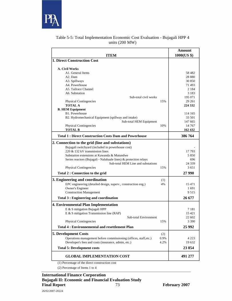
International Finance Corporation Bujagali II: Economic and Financial Evaluation Study Final Report 73 February 2007 26/02/2007-20224
Table 5-5: Total Implementation Economic Cost Evaluation - Bujagali HPP 4 units (200 MW)
ITEM Amount
1000(US $) 1. Direct Construction Cost
A. Civil WorksA1. General Items 58 482 A2. Dam 28 880 A3. Spillways 30 850 A4. Powerhouse 71 493 A5. Tailrace Channel 2 184 A6. Substation 3 183
Sub-total civil works 195 071 Physical Contingencies 15% 29 261 TOTAL A 224 332
B. HEM EquipmentB1. Powerhouse 114 165 B2. Hydromechanical Equipment (spillway and intake) 33 501
Sub-total HEM Equipment 147 665 Physical Contingencies 10% 14 767 TOTAL B 162 432
Total 1 : Direct Construction Costs Dam and Powerhouse 386 764
2. Connection to the grid (line and substations)Bujagali switchyard (included in powerhouse cost) - 220 & 132 kV transmission lines 17 793 Substation extensions at Kawanda & Mutundwe 5 850 Series reactors (Bujagali - Nalubaale lines) & protection relays 696
Sub-total HEM Line and substations 24 339 Physical Contingencies 15% 3 651
Total 2 : Connection to the grid 27 990
3. Engineering and coordination (1)EPC engineering (detailed design, superv., construction eng.) 4% 15 471 Owner's Engineer 1 691 Construction Management 9 515
Total 3 : Engineering and coordination 26 677
4. Environmental Plan ImplementationE & S mitigation Bujagali HPP 7 181 E & S mitigation Transmission line (RAP) 15 421
Sub-total Environment 22 602 Physical Contingencies 15% 3 390
Total 4 : Environnemental and resettlement Plan 25 992
5. Development Costs (2)Operations management before commissioning (offices, staff,etc.) 0.9% 4 223 Developer's fees and costs (insurance, admin, etc.) 4.2% 19 632
Total 5: Development costs 23 854
GLOBAL IMPLEMENTATION COST 491 277 (1) Percentage of the direct construction cost(2) Percentage of Items 1 to 4
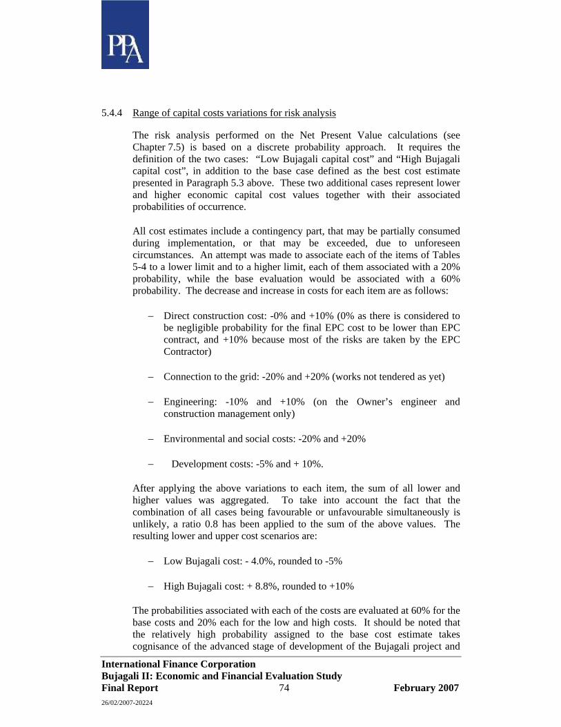
International Finance Corporation Bujagali II: Economic and Financial Evaluation Study Final Report 74 February 2007 26/02/2007-20224
5.4.4 Range of capital costs variations for risk analysis
The risk analysis performed on the Net Present Value calculations (see Chapter 7.5) is based on a discrete probability approach. It requires the definition of the two cases: “Low Bujagali capital cost” and “High Bujagali capital cost”, in addition to the base case defined as the best cost estimate presented in Paragraph 5.3 above. These two additional cases represent lower and higher economic capital cost values together with their associated probabilities of occurrence.
All cost estimates include a contingency part, that may be partially consumed during implementation, or that may be exceeded, due to unforeseen circumstances. An attempt was made to associate each of the items of Tables 5-4 to a lower limit and to a higher limit, each of them associated with a 20% probability, while the base evaluation would be associated with a 60% probability. The decrease and increase in costs for each item are as follows:
− Direct construction cost: -0% and +10% (0% as there is considered to be negligible probability for the final EPC cost to be lower than EPC contract, and +10% because most of the risks are taken by the EPC Contractor)
− Connection to the grid: -20% and +20% (works not tendered as yet)
− Engineering: -10% and +10% (on the Owner’s engineer and construction management only)
− Environmental and social costs: -20% and +20%
− Development costs: -5% and + 10%.
After applying the above variations to each item, the sum of all lower and higher values was aggregated. To take into account the fact that the combination of all cases being favourable or unfavourable simultaneously is unlikely, a ratio 0.8 has been applied to the sum of the above values. The resulting lower and upper cost scenarios are:
− Low Bujagali cost: - 4.0%, rounded to -5%
− High Bujagali cost: + 8.8%, rounded to +10%
The probabilities associated with each of the costs are evaluated at 60% for the base costs and 20% each for the low and high costs. It should be noted that the relatively high probability assigned to the base cost estimate takes cognisance of the advanced stage of development of the Bujagali project and

International Finance Corporation Bujagali II: Economic and Financial Evaluation Study Final Report 75 February 2007 26/02/2007-20224
the fact that the EPC contract has already been tendered and is under the final stages of negotiation. Equal probabilities are assigned to the high and low costs variations since each is considered equally likely given that the estimates assumed a skewed variation in the costs about the base value.
5.5 Karuma HPP
5.5.1 Characteristics of the project
The description of the various components of the Karuma Falls Hydropower Project have been found in the Project Definition Report (March 1999) issued by Norpak. The scheme is a run-of-the-river type, with no active storage, using the natural head created by the Karuma Falls and adjacent rapids, immediately upstream of the bridge across the Victoria Nile
The developer of Karuma HPP is NORPAK, who has been invited to negotiate a Power Purchase Agreement by GoU in 2004. Norpak has been promoting the project since the 1990's and has recently confirmed to GoU its interest in developing the project at attractive financial conditions.
The initial proposal of the developer was to implement the project with an installed capacity of either 150 or 200 MW, generated by 3 or 4 units of 50 MW capacity each. As 3 units would be able to use only about 600 m3/s from the inflow of the Victoria Nile, system planning studies will most probably show that at least 4 units should be installed.
In the case of High hydrology inflow, a roughly constant discharge around 1250 m3/s would be released from Lake Victoria for years, and most of it would be available for power generation at Karuma. This explains why, as presented in Section 3 above, the calculation of the energy generation capability of Karuma HPP has also been calculated for 5 and 6 units, which could generate 250 and 300 MW respectively (with a maximum discharge of 1000 and 1200 m3/s respectively).
The works at Karuma HPP would essentially comprise:
• an overflow weir across the Nile, upstream of the Karuma Falls,
• a short intake, directly connected to an underground powerhouse in the left bank,
• for each of the units, one surge chamber (section 73 m2), approximately 500 m long, and one tailrace tunnel (section 150 m2), approximately 2 km long, leading to the outlet in the left bank;
• a number of access tunnels and access roads, and
• a switchyard located on the left bank.
International Finance Corporation Bujagali II: Economic and Financial Evaluation Study Final Report 76 February 2007 26/02/2007-20224
According to the Project Definition Report (DPR), the blasting of some protruding parts of the river bed between the outlet and the Karuma bridge could lower the Tail Water Level at least by one metre.
The geology of the area in which most of the underground works will be performed is "gneisses of medium strength" according to the geological interpretation of site investigations, found in the DPR. No major fault has been identified in the project area, but the designers note that "the tunnels will intersect several intermediate and minor faults and weathered weakness zones". The fact that the tunnels and powerhouse cavern will be excavated relatively close to the surface is not in favour of the stability of the excavation for two reasons, correctly identified in the DPR: i) low vertical stresses, that usually improve the stabilisation of the excavation when the depth increases, ii) increased likelihood and frequency of highly jointed and weathered zones, that will require heavier stabilisation measures to be taken.
The quantities of the main works and the main characteristics of the works at Karuma are summarised in Table 5-3.
This table shows that the main difference with Bujagali works consists of:
• a large volume of underground excavation, to be performed in relatively difficult geological and topographical context at Karuma, while there is no underground work at Bujagali,
• a smaller volume of concrete work at Karuma than at Bujagali.
5.5.2 Construction costs
The economic cost of construction of Karuma HPP has been evaluated on the basis of the following data and assumptions:
• Design and drawings shown in the Project Definition Report (March 1999);
• Additional memo received in February 2006 from Norplan, showing the main volumes of works,
• Unit rates of civil works and power plant equipment obtained from recent international bidding on similar works, consistent with the rates used for Bujagali cost estimates;
• All costs are expressed in US$, value January 2006, excluding all taxes and duties.
The main volumes of work have been checked for the main items such as the volume of underground works and the volume of the weir, and they have been found in fairly good agreement with the volumes indicated by Norplan.

International Finance Corporation Bujagali II: Economic and Financial Evaluation Study Final Report 77 February 2007 26/02/2007-20224
Costs are presented for Karuma equipped in a single stage with four units of 50 MW each.
The resulting construction costs are presented in Table 5-6 below, together with the total implementation cost.
5.5.3 Other costs and resulting total cost of implementation
In addition to direct construction costs, other costs include, as for Bujagali:
• the costs of all engineering activities, evaluated in the context of an EPC contract, including the cost of an Independent Consultant to guarantee the quality of the design and construction work of the EPC contractor;
• environmental and social impact costs; and
• other development costs linked to financing fees, developer's fees, etc., with the same uncertainties as for Bujagali.
The environmental and social costs have been estimated by the Consultant’s specialists following a visit to Uganda in July 2006. During their time in Uganda they visited the Karuma site and held discussions with the various authorities and stakeholders. Details of the build-up of the E&S costs included in Table 5-6 are presented in Section 6.
As shown in the table below, various rates have been applied for physical contingencies, to cater for the additional works that unavoidably arise during construction, above the volumes measured at an early stage of design. The ratios are usually selected between 5% and 20%, depending on the nature of the works and the degree of confidence in the available data. Among them, the ratio of 20% has been considered for the civil works at Karuma, against 15% at Bujagali, because the cost of underground works at Karuma is much less predictable than the surface works at Bujagali. At this stage of evaluation, it was considered the best way to take into account the difference in risk during construction between the two projects.
The Karuma cost estimate shown in Table 5-6 excludes interest during construction.
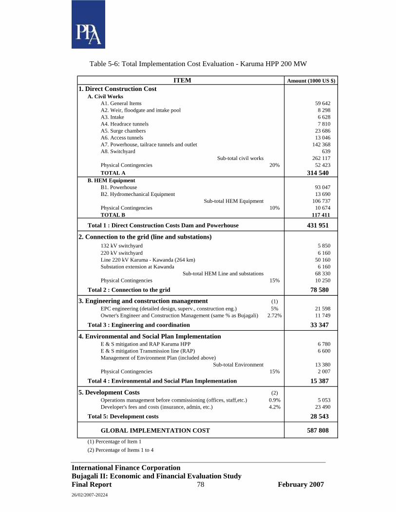
International Finance Corporation Bujagali II: Economic and Financial Evaluation Study Final Report 78 February 2007 26/02/2007-20224
Table 5-6: Total Implementation Cost Evaluation - Karuma HPP 200 MW
ITEM Amount (1000 US $)1. Direct Construction Cost
A. Civil WorksA1. General Items 59 642 A2. Weir, floodgate and intake pool 8 298 A3. Intake 6 628 A4. Headrace tunnels 7 810 A5. Surge chambers 23 686 A6. Access tunnels 13 046 A7. Powerhouse, tailrace tunnels and outlet 142 368 A8. Switchyard 639
Sub-total civil works 262 117 Physical Contingencies 20% 52 423 TOTAL A 314 540
B. HEM EquipmentB1. Powerhouse 93 047 B2. Hydromechanical Equipment 13 690
Sub-total HEM Equipment 106 737 Physical Contingencies 10% 10 674 TOTAL B 117 411
Total 1 : Direct Construction Costs Dam and Powerhouse 431 951
2. Connection to the grid (line and substations)132 kV switchyard 5 850 220 kV switchyard 6 160 Line 220 kV Karuma - Kawanda (264 km) 50 160 Substation extension at Kawanda 6 160
Sub-total HEM Line and substations 68 330 Physical Contingencies 15% 10 250
Total 2 : Connection to the grid 78 580
3. Engineering and construction management (1)EPC engineering (detailed design, superv., construction eng.) 5% 21 598 Owner's Engineer and Construction Management (same % as Bujagali) 2.72% 11 749
Total 3 : Engineering and coordination 33 347
4. Environmental and Social Plan ImplementationE & S mitigation and RAP Karuma HPP 6 780 E & S mitigation Transmission line (RAP) 6 600 Management of Environment Plan (included above)
Sub-total Environment 13 380 Physical Contingencies 15% 2 007
Total 4 : Environmental and Social Plan Implementation 15 387
5. Development Costs (2)Operations management before commissioning (offices, staff,etc.) 0.9% 5 053 Developer's fees and costs (insurance, admin, etc.) 4.2% 23 490
Total 5: Development costs 28 543
GLOBAL IMPLEMENTATION COST 587 808 (1) Percentage of Item 1(2) Percentage of Items 1 to 4

International Finance Corporation Bujagali II: Economic and Financial Evaluation Study Final Report 79 February 2007 26/02/2007-20224
5.6 Other Candidate Hydro
5.6.1 Other major hydro power projects
A review of the potential large hydroelectric projects in Uganda was made in the 2001 Acres study, based on existing studies such as the 1997 Master Plan. The conclusions of this review were that, in addition to Bujagali and Karuma that had already been studied at feasibility level, the only sites that were considered particularly attractive for the development of the Uganda power system were: Kalagala, Ayago, Murchison and Masindi.
Three among these four hydroelectric projects were eliminated by Acres in 2001 for reasons that are still valid today:
• Ayago and Murchison, both located downstream of Karuma, in the middle of the Murchison Falls National Park, have been the subject of studies concluding that they are technically feasible projects. Nevertheless, both of them are penalized by the environmental impacts they could cause in the National Park, and they cannot be considered as potential alternatives to Bujagali or Karuma for an implementation starting in the coming years.
• Masindi would appear to have been studied only at a conceptual level, and its large size (up to 3000 MW) makes it a too large project for being considered in the Uganda power system in the next ten years.
The fourth project is Kalagala, located approximately 15 km downstream of Bujagali. According to the pre-feasibility studies performed on this site, the project seems to be technically and economically attractive. Nevertheless, its environmental and social impacts aggregated with the impacts of Bujagali were found to be unacceptable. As a consequence, and parallel with the development of Bujagali HPP, GoU decided that no hydroelectric project should ever be developed on this site (ref.: "Kalagala offset").
Bujagali and Karuma therefore appear to be the only major hydro power candidates that can be developed in the coming years to contribute to meeting the power demand in the country by mobilising the renewable energy of the Nile.
5.6.2 Small and Medium Scale Hydro
The small hydro projects that are included in the least cost planning analysis are presented in Section 4.4. In the absence of firm information and studies, no other small hydro projects have been included in the least cost planning analysis. The impact on the least cost plan, and on the Bujagali project, of any

International Finance Corporation Bujagali II: Economic and Financial Evaluation Study Final Report 80 February 2007 26/02/2007-20224
other projects that may be developed over the coming years is likely to be relatively small.

International Finance Corporation Bujagali II: Economic and Financial Evaluation Study Final Report 81 February 2007 26/02/2007-20224
6 Environmental and Social Costs
6.1 Introduction
The consultant’s social and environmental specialists visited Uganda in July 2006. The visit had to be made in advance of the completion of new ESIA for Bujagali by Burnside Consultants for the developer, BEL. The ESIA has been completed since the Draft Final Report was submitted and this Final Report takes account of the results of the ESIA report.
6.2 Environmental Costs and Benefits of Bujagali
6.2.1 Dam and Power Station
In the Environmental Impact Assessment for the Hydro Project and the Environmental Impact Statement for the Transmission System prepared by ESG International and WS Atkins International March 2001, environmental costs have being identified and incorporated in the total project cost.
These costs cover mitigation, compensation, offset measures, monitoring of impacts and environmental reporting. Costs for environmental management during the construction phase were said to be included in the construction cost estimates. It would be useful to identify these costs clearly in the construction budget as this is not possible at the moment.
For Bujagali dam, reservoir and power-station, the amount budgeted for environment in 2001 is US$ 360,000. This includes US$ 300,000 for the implementation of the Environmental Management Plan, US$ 20,000 for an environmental panel, US$ 20,000 for a forestry laboratory, and US$ 20,000 for institutional improvements.
Based on our review to-date, we consider that to safeguard the environment according to the IFC policies, the budget for environmental measures must be increased as follows:
EMP during construction US$ 600,000
Social/Environmental Review Panel US$ 120,000
Environmental impacts monitoring during construction US$ 250,000
Provision for unexpected impacts US$ 300,000
Forestry laboratory US$ 70,000
Institutional Improvements US$ 70,000
Total updated environmental budget US$ 1,410,000
In addition, US$ 50,00 per year should be budgeted for an environmental management programme (EMP) throughout the operating life of the project
International Finance Corporation Bujagali II: Economic and Financial Evaluation Study Final Report 82 February 2007 26/02/2007-20224
and a further US$ 50,000 per year for the first five years of operation for the monitoring of impacts relating specifically to fish population and fisheries.
The costs presented in the Burnside Report are as follows:
Staffing for SEAP Implementation US$ 1,125,000
S&E panel of experts US$ 300,000
Mitigation of biophysical impacts, not construction related US$ 2,159,080
Comprising:
- US$ 321 000 during the preconstruction phase - US$ 1 476 200 during construction - US$ 361,880 during operation (first 2 years)
Total budget US$ 3,584,080
This declared budget of US$3.58 million should be sufficient to cover the environmental cost of the dam and power house and was used in the economic analysis.
6.2.2 Transmission Line
A budget of US$ 587,000 is included in the 2001 studies for the transmission line. It is considered that this should be increased by a further US$ 100,000 to allow for unexpected impacts in the event of major changes to the original transmission line route. Note: this budget is slightly higher than the US$485,000 budget estimated by Burnside for the implementation of environmental mitigation measures associated with the Bujagali transmission line. This small difference will not have a significant impact on the economic and financial analysis.
Details of the environmental budget are shown in Table 6-1, and the estimated phasing of the expenditure covering both the dam and power house and the transmission line in Table 6-2.

International Finance Corporation Bujagali II: Economic and Financial Evaluation Study Final Report 83 February 2007 26/02/2007-20224
Table 6-1: Environmental Mitigation Budget for Bujagali Transmission Line
Item Estimate (US$’000)
Environmental Management 40
Environmental Review Panel 27
Institutional Strengthening 20
Forest Habitat Biodiversity * 220
Enrichment Planting at Mabira Forest 280
Unexpected impacts 100
Total for transmission line 687
* - implement forest offset proposal at Kalagala Falls and proposal at Mabira Forest.
Table 6-2: Estimated Phased Environmental Costs (US$’000)
Item 2007 2008 2009 2010 Total
Dam & power house 0.89 0.78 0.78 1.11 3.56
Transmission line 0.23 0.23 0.23 0.69
Sub-total 1.12 1.01 1.01 1.11 4.25
Contingencies (15%) 0.18 0.15 0.15 0.16 0.64
Total 1.30 1.16 1.16 1.27 4.89
6.2.3 Environmental Benefits
The amounts of avoided CO2 for Bujagali are substantial. Table 6-3 shows the avoided CO2 compared with medium speed diesel plant for the low and high hydrology release outputs of Bujagali with five units. The value of the avoided CO2 will vary depending on the actual mix of thermal plant at the time. The impact on the Bujagali EIRR of avoided carbon dioxide emissions is evaluated in Section 8.
Table 6-3: Bujagali - Potential Carbon Dioxide Emissions Avoided
Low hydrology High hydrology
GWh/year CO2 avoided (tonne’000/year)
GWh/year CO2 avoided (tonne’000/year)
1,165 822 1,991 1,405

International Finance Corporation Bujagali II: Economic and Financial Evaluation Study Final Report 84 February 2007 26/02/2007-20224
In the economic analysis the value of CO2 avoided has been based on US$25/tonne which is in the lower band of the equilibrium level quoted in the recent Stern Report on climate change.
There may be SOx impacts but the value of SOx emissions has not been quantified in the economic and financial analysis.
6.3 Social Costs and Benefits of Bujagali
6.3.1 Compensation and Resettlement of Dam and Power House
The RAP for Bujagali I showed a compensation and resettlement budget of US$ 11.13 million. The compensation and resettlement component of Bujagali I has been all but completed and the above amount has been all but disbursed prior to Bujagali II being formulated. Hence these costs can be considered sunk, and therefore will not need to be included in the estimates for Bujagali II.
There are however some relatively minor resettlement issues still to be finalized. Eighteen households were not yet paid, mostly on account of the requisite bank accounts not yet having been opened. The amounts involved are small. The fencing of the project property on the east bank is still to be carried out, and a contract to do this has been let, at a cost of US$ 30,000.
All the titles to new plots of land now occupied by relocatees have not yet been issued by the authorities. These legal and administrative procedures need to be completed; the actual cost of doing so can be considered as government overhead.
Burnside carried out a June 2006 Audit of the compensation and resettlement tasks completed to that date, showing any outstanding resettlement items and the cost involved in dealing with this. The Burnside report6 shows a budget of US$ 497,000 covering the outstanding resettlement issues. Of this amount, US$ 320,000 is included in the CDAP, for three livelihood improvement activities: agriculture, fisheries and small businesses. Therefore, the net amount for the compensation and resettlement component is US$ 177,000.
The APRA indicates that provision of electricity was not considered for the Resettlement Area. However, the report states that “BEL will discuss possible provision of power to the resettlement area.” No budget allowance is made for this, although certain “provisions” are included in the CDAP budget – see below.
6 “Assessment of Past Resettlement Activities” (APRA)

International Finance Corporation Bujagali II: Economic and Financial Evaluation Study Final Report 85 February 2007 26/02/2007-20224
A social monitoring unit to will be established within the BIU. While this is certainly appropriate, it will not obviate the need for independent monitoring and evaluation. BEL will also set up a social unit, the budget for which is included in the CDAP budget (US$ 361,000).
6.3.2 Community Development Action Plan – CDAP
Compared to compensation and resettlement, little progress has been made with the implementation of the Bujagali I CDAP. In summary, eight wells were provided under the water resources component of the Plan. However, some of these wells did not perform and now have to be replaced.
The Burnside Audit also dealt with current community needs and provided updated estimates of the cost of specific measures. The total CDAP budget in Bujagali I was US$ 1,825,500. We were not able to establish exactly how much of this budget has been disbursed in each category, although BIU promised to supply rough estimates. The Burnside Audit sheds little light on this. However, whatever little has been spent is considered as a sunk cost.
A comparison between the CDAP for Bujagali I and Bujagali II, based on the estimates in the Burnside December 2006 SEA –Appendix J is shown in Table 6-4.
There are a number of notable differences between the Bujagali I and the Bujagali II components of the CDAP budget. In particular, the recognition of the agricultural needs of the project area, the substantially increased cost of implementation, the decreased allowances for health and education, and the total absence of direct rural electrification, stand out.
The December 2006 Burnside SEA main report indicates a total CDAP budget of US$ 3,817,000. The difference between the US$ 2,549,000 above and the total budget is US$ 1,268,000.
According to Burnside, the US$ 1,268,000 includes the following items:
“ - provision for an electrification feasibility study
- provision for tourism development at Kalagala
- provision for Equator and Nalubaale Rafting initiatives
- provision for additional tree planting and monitoring, weed release and tending at Kalagala
- provision for additional education, health and electricity initiatives.
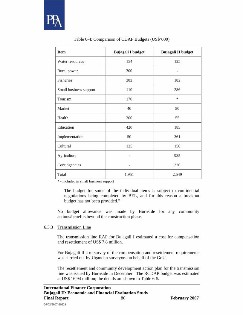
International Finance Corporation Bujagali II: Economic and Financial Evaluation Study Final Report 86 February 2007 26/02/2007-20224
Table 6-4: Comparison of CDAP Budgets (US$’000)
Item Bujagali I budget Bujagali II budget
Water resources 154 125
Rural power 300 -
Fisheries 282 182
Small business support 110 286
Tourism 170 *
Market 40 50
Health 300 55
Education 420 185
Implementation 50 361
Cultural 125 150
Agriculture - 935
Contingencies - 220
Total 1,951 2,549
* - included in small business support
The budget for some of the individual items is subject to confidential negotiations being completed by BEL, and for this reason a breakout budget has not been provided.”
No budget allowance was made by Burnside for any community actions/benefits beyond the construction phase.
6.3.3 Transmission Line
The transmission line RAP for Bujagali I estimated a cost for compensation and resettlement of US$ 7.8 million.
For Bujagali II a re-survey of the compensation and resettlement requirements was carried out by Ugandan surveyors on behalf of the GoU.
The resettlement and community development action plan for the transmission line was issued by Burnside in December. The RCDAP budget was estimated at US$ 16,94 million; the details are shown in Table 6-5.

International Finance Corporation Bujagali II: Economic and Financial Evaluation Study Final Report 87 February 2007 26/02/2007-20224
There is an indicative budget of US$ 300,000 for CDAP activities along the transmission line. On this basis, each community would receive some US$ 5,000. A formula to allocate the CDAP budget is provided in the RCDAP, taking into account population and length of transmission line for each community. The RCDAP cost would be borne by GoU.
Table 6-5: Details of RCDAP budget
Item Budget (US$ million)
Resettlement sites and housing 2.93
Cash compensation 9.08
Livelihood restoration 0.30
Implementation 2.12
Community development 0.30
Sub-total 14.73
Contingencies (15%) 2.21
Total 16.94
6.3.4 Social costs by year
Based on a start of construction in 2007, and a four year construction period, the social costs would be expended approximately as shown in Table 6-6.
Table 6-6: Estimated Phased Social Costs (US$’000)
Item 2007 2008 2009 2010 Total
Dam & power house 0.60 1.21 1.21 0.60 3.62
Transmission line 4.21 4.21 4.21 2.10 14.73
Sub-total 4.81 5.42 5.42 2.70 18.35
Contingencies (15%) 0.72 0.81 0.81 0.41 2.75
Total 5.53 6.23 6.23 3.11 21.10

International Finance Corporation Bujagali II: Economic and Financial Evaluation Study Final Report 88 February 2007 26/02/2007-20224
6.4 Environmental Costs and Benefits of Karuma
6.4.1 Introduction
The information and estimates were prepared by the PPA environmental and social consultants following a field visit to Uganda in July 2006, and make reference to the Karuma Falls EIA.7, prepared in 1999.
Details of the Karuma project are included in Section 5.5. Karuma Falls lie in central North Uganda 260km north of Kampala on the Victoria Nile, 80km downstream of Lake Kyoga. The Kampala-Gulu road passes about 3 km to the west of the proposed site. The access road will branch off the main road 100 m north of the Karuma Trading Centre.
The project is expected to comprise four generating units, each of 50 MW capacity. No dam would be built but, instead, a low concrete overflow weir 190 m long would be constructed to maintain a stable water level at the power station intake about 3.5 m above the natural river level. The weir would be submerged with a minimum flow of 50 m3/s at all times. An underground powerhouse would be built on the south bank of the river with underground headrace tunnels and four underground 2.2 km long tailrace tunnels. These tailrace tunnels would return the diverted waters to the river below the Karuma Falls. There would be no reservoir and no impoundment. A water level increase of 0-40 cm would occur at the rapids 3.5 km upstream the weir. Only about 1.8 ha of land would be inundated.
Two camps, one permanent and one for the construction period, would be built on the south bank near Awoo village. Most of the project activities would take place on the south bank with an access road connecting with the Kampala Guru road and a 1 km access road from the existing Karuma bridge would connect the weir conduction site on the north bank.
The switchyard would be located on the south bank near the underground power station. A 75 km 132 kV line would join the existing grid along the road from Lira to Kampala. A 264 km double circuit 220 kV line is proposed through Masindi to Kawanda substation, near Kampala. Two 33 kV lines would take electricity from the switchyard to the trading centres of Karuma and Kamdini.
A work force of around 500-700 non skilled and 100 skilled workers would be required for the construction of the project.
7 Prepared for NORPAK Power Limited, dated May 1999.
International Finance Corporation Bujagali II: Economic and Financial Evaluation Study Final Report 89 February 2007 26/02/2007-20224
6.4.2 Environmental Impacts
The main environmental impacts are expected to include:
• Increase water level for the first 300 m upstream of the weir (+2.5-3 m).
• 1.8 ha of river bed land upstream of the weir inside the actual river banks would be permanently inundated.
• Reduced river flow along almost 3 km long stretch; a minimum bypass flow of 50 m3/s is recommended. However it is expected that the flow in the by-passed section would, most of the time, be greater, depending on the installed capacity and the Nile hydrology.
• There is a hippo population in the river and in the reduced flow section; some hippo habitat would be affected as well as some crocodile and water cobra habitats. The location and extent of suitable habitat for amphibians would be modified in this section, depending on wetland vegetation increase or decrease.
• Parts of the river bed would become dry for at least part of the year and former fast flowing sections would become more suitable for aquatic species adapted to slow flowing water and species adapted to fast flowing water would experience a local habitat decrease.
• Fish migration: The weir would likely act as a barrier for upstream short distance migrations. Murchison Falls (natural) and the Owen Falls Dam (man-made) act presently as barriers for long distance migration to lakes Kyoga and Victoria.
• The land on the south bank where camps and switchyard are to be build is already highly modified and cultivated. No significant impacts are expected. However hippos forage during the night in the farmers fields.
• There would be an increased risk of water contamination during the construction period and the operation period, mainly from sediment, oil and fuel spills, and chemical products.
6.4.3 Social Impacts
The main social impacts are expected to include:
• 35 households would be directly affected and would need to be resettled: 30 at Awoo village and 5 at Nora village. Temporary cultivated land losses would be 120 ha at Awoo construction site, camps, access roads and switchyard, and 15 ha at Nora village on the
International Finance Corporation Bujagali II: Economic and Financial Evaluation Study Final Report 90 February 2007 26/02/2007-20224
North bank for access road and weir construction site. Permanent land losses would be about 45 ha. There is already a shortage of arable land in the region due to the number of refugees.
• To this number are to be added the impacted households and cultivated land requirements inside the rights of way for the transmission line network of 315 km for the 132 and 220 kV lines. Sixty km of these new transmission routes are said to be heavily settled. However fewer problems are expected than with the Bujagali transmission network.
• On the south bank, the 30 affected households (living in mud huts) and the required 120 ha have already being compensated and acquired. However people still live there and continue their subsistence farming. US $150,000 has already been spent on compensation.
• The project is located in, or borders, five villages. In 1998 the total estimated number of households was 1669. Karuma village is the nearest trading centre, market and transportation and service centre. Many of the inhabitants are displaced people from the northern districts.
• There are no suitable sanitation provisions. There is no safe drinking water and no electricity. The population in the five villages does not have any land title documents.
• The existing education facilities are highly inadequate and unable to cope with the population increase. Norplan estimates that a population increase in the project area of 60% could materialize, thus adding 3500-4000 persons to the existing 6000 inhabitants of the area.
• People practise subsistence farming and rely heavily on the rivers (59% of the interviewed people said that they ate fish more than once a week). Water usage for fishing, bathing and washing and the source of drinking water on the south bank would be affected.
• Increased demand for fuel wood would further threaten the nearby Wildlife Reserve and National Park. Health facilities in the project area are inadequate or non-existent. STDs are very common and prostitution is already prevalent.
• The local population might be able to get temporary employment during the construction phase if the developer prescribes pro-active hiring and training policies. But the permanent work force is expected to be below 30 people.
• Local businesses might benefit from the project during its construction.

International Finance Corporation Bujagali II: Economic and Financial Evaluation Study Final Report 91 February 2007 26/02/2007-20224
• The view of the Karuma Falls would be modified, except during flood periods. It is a succession of beautiful rapids, but Karuma does not have spectacular falls such as can be seen at Murchison. The transmission line visual impacts would be noticeable all along the Kampala – Guru Road up to Kampala.
6.4.4 Mitigation and Compensation Measures
Environmental measures
• A re-vegetation programme would be defined and introduced;
• Measures should be introduced to safeguard the forest in the WRNR. The local population and workers would be supplied with fuel wood. A programme to establish woodlots should be initiated;
• The staff of the Murchison Falls Conservation complex should be strengthened by 10 to15 new staff members plus equipment;
• A minimum bypass flow of 50m3/s would be maintained (estimated value US$ 5 million per year);
• small overflow weirs should be constructed in the 3.5 km of reduced flows stretch;
• A fish passage might be needed;
• A monitoring programme should be implemented during the construction and operation phases to monitor impacts on river water quality, river flow, terrestrial vegetation, conservation areas, birds, hippos, crocodiles, amphibians, and other wildlife populations; and
• Fish populations should also be monitored, as well as the effectiveness of a fish passage is this is mandated.
Social Measures
• Preventive health measures: awareness campaign, distribution of treated mosquito nets, control of pools of water to prevent insect proliferation;
• Creation of a permanent health centre for workers and local population;
• Creation of an Agricultural Intensification programme;
• Measures need to be taken to assure safe water for the population: boreholes and pumps or other form of supply for the five villages in the project area as a general compensation measure;

International Finance Corporation Bujagali II: Economic and Financial Evaluation Study Final Report 92 February 2007 26/02/2007-20224
• Electrification. The feasibility study states that “It is unlikely that electricity would be economically and physically (made) available for the majority of the local people. However, electrification is recommended for the Karuma and Kamdini Trading centres.” This position should be re-examined, as electrification of the project area, in one form or another, is deemed to be the most important benefit that an electricity project can bestow on the nearby population in order to combat poverty;
• Employment: local people should be given priority and women should be given a percentage of the manual work available during construction;
• To ensure peaceful co-existence of villagers and newcomers there is a need for a police post in Karuma and a Grievance Committee;
• The feasibility study indicates that for traffic safety reasons, people living in a buffer zone of 50m along the access roads should be resettled and compensated. In our view this may not be in keeping with the ROW provisions of the national roads department. Furthermore it would impose unnecessary hardship on those thus affected. More suitable might be inconvenience allowances to be paid during the period of construction of the project, to compensate for noise, dust, etc.
• A policy of land for land compensation for loss of arable land is recommended; lost crops would be paid for in cash;
• A savings credit scheme run by an NGO could provide the local people with a chance to benefit from the influx of people; and
• Monitoring of the human environment would focus on economic and health issues. Resettlement of 200 peoples (35 households) and compensation for land and agricultural losses should be closely monitored. An ongoing health monitoring programme should be put in place for the local population and workers. Capacity of school facilities to cope with the influx should be monitored. Employment for the local population, agricultural production, housing and facilities for the workers, inflation of food and fuel prices should also be monitored.
6.4.5 Environmental and Social Costs
A budget of US $1,935,000 has been identified in NORPAK EIA for the project environmental impacts mitigation and monitoring programme. The estimated costs of environmental monitoring and mitigation measures are shown in Table 6-7.
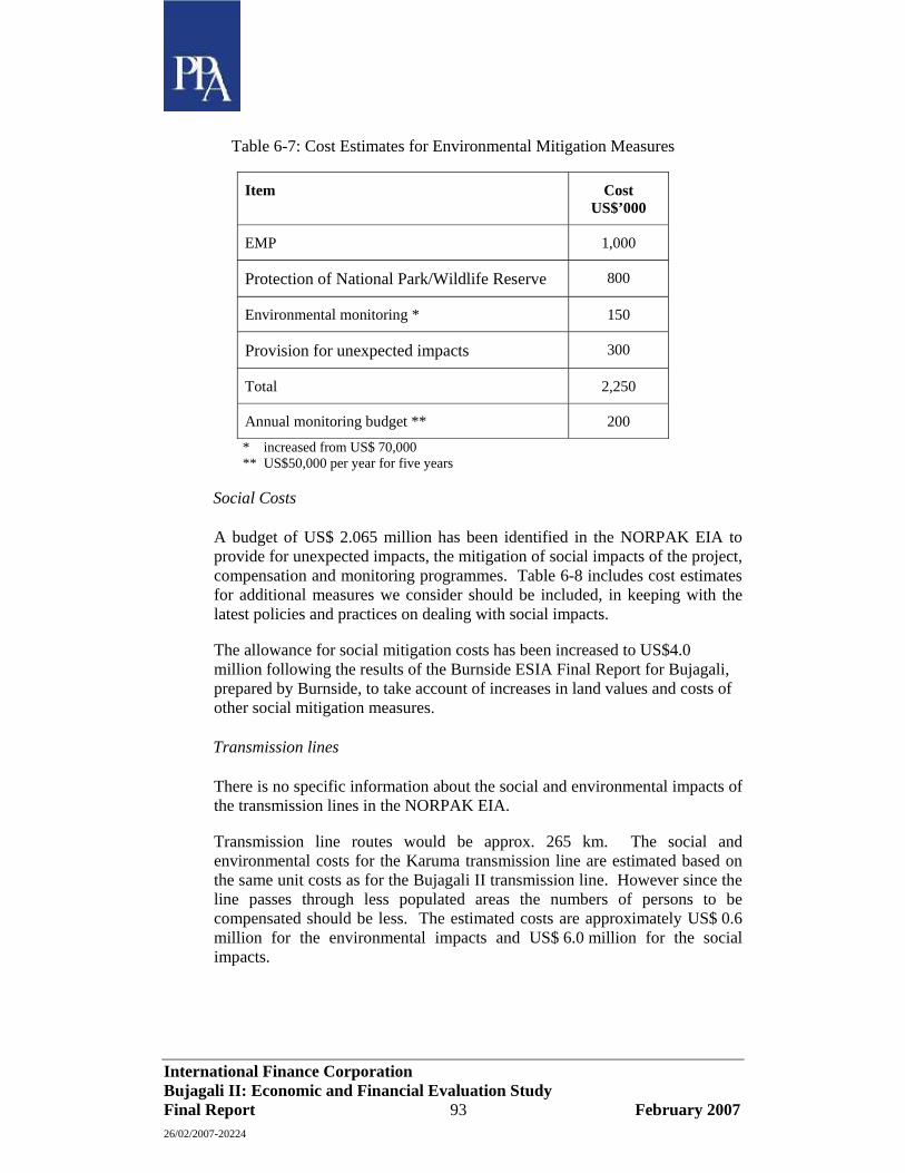
International Finance Corporation Bujagali II: Economic and Financial Evaluation Study Final Report 93 February 2007 26/02/2007-20224
Table 6-7: Cost Estimates for Environmental Mitigation Measures
Item Cost US$’000
EMP 1,000
Protection of National Park/Wildlife Reserve 800
Environmental monitoring * 150
Provision for unexpected impacts 300
Total 2,250
Annual monitoring budget ** 200
* increased from US$ 70,000 ** US$50,000 per year for five years
Social Costs
A budget of US$ 2.065 million has been identified in the NORPAK EIA to provide for unexpected impacts, the mitigation of social impacts of the project, compensation and monitoring programmes. Table 6-8 includes cost estimates for additional measures we consider should be included, in keeping with the latest policies and practices on dealing with social impacts.
The allowance for social mitigation costs has been increased to US$4.0 million following the results of the Burnside ESIA Final Report for Bujagali, prepared by Burnside, to take account of increases in land values and costs of other social mitigation measures.
Transmission lines
There is no specific information about the social and environmental impacts of the transmission lines in the NORPAK EIA.
Transmission line routes would be approx. 265 km. The social and environmental costs for the Karuma transmission line are estimated based on the same unit costs as for the Bujagali II transmission line. However since the line passes through less populated areas the numbers of persons to be compensated should be less. The estimated costs are approximately US$ 0.6 million for the environmental impacts and US$ 6.0 million for the social impacts.
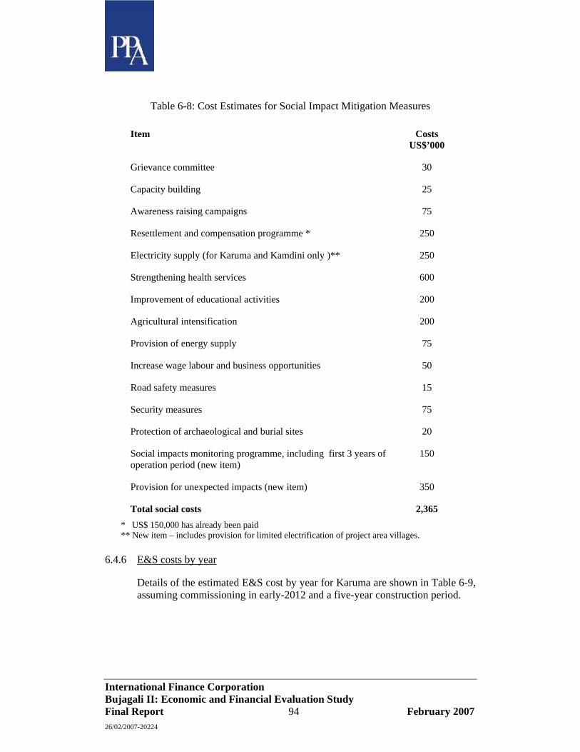
International Finance Corporation Bujagali II: Economic and Financial Evaluation Study Final Report 94 February 2007 26/02/2007-20224
Table 6-8: Cost Estimates for Social Impact Mitigation Measures
Item Costs US$’000
Grievance committee 30
Capacity building 25
Awareness raising campaigns 75
Resettlement and compensation programme * 250
Electricity supply (for Karuma and Kamdini only )** 250
Strengthening health services 600
Improvement of educational activities 200
Agricultural intensification 200
Provision of energy supply 75
Increase wage labour and business opportunities 50
Road safety measures 15
Security measures 75
Protection of archaeological and burial sites 20
Social impacts monitoring programme, including first 3 years of operation period (new item)
150
Provision for unexpected impacts (new item) 350
Total social costs 2,365 * US$ 150,000 has already been paid ** New item – includes provision for limited electrification of project area villages.
6.4.6 E&S costs by year
Details of the estimated E&S cost by year for Karuma are shown in Table 6-9, assuming commissioning in early-2012 and a five-year construction period.

International Finance Corporation Bujagali II: Economic and Financial Evaluation Study Final Report 95 February 2007 26/02/2007-20224
Table 6-9: Estimated Phasing of Environmental and Social Costs (US$’000)
Item 2007 2008 2009 2010 2011 Total
Environmental costs- Dam & Power House
EMP 200 200 200 200 200 1,000
Review panel 24 24 24 24 24 120
Environmental impact monitoring * - 50 50 50 50 200
Provision for unforeseen impacts 100 100 100 300
National Park wildlife protection 200 200 200 200 800
Total 224 474 574 574 574 2,420
Social costs - Dam & Power House
Compensation and resettlement 800 800 800 800 800 4,000
Total 800 800 800 800 800 4,000
Transmission line
Environmental costs - - 200 200 200 600
Social costs - - 3,000 3,000 6,000
Total - - 200 3,200 3,200 6,600
Contingencies (15%) 154 191 236 686 686 1,953
Total E & S Costs 1,178 1,465 1,810 5,260 5,260 14,973
* plus US$ 180,000 per year for first 2 years of operation environmental impact monitoring, adds US$312,000 to the cost in 2011 in PW terms.
6.4.7 Environmental Benefits
The amounts of avoided CO2 for Karuma are substantial. Table 6-10 shows the avoided CO2 compared with medium speed diesel plant for the low and high hydrology release outputs of Karuma with four units. The value of the avoided CO2 would vary depending on the actual mix of thermal plant at the time.
Table 6-10: Karuma - Potential Carbon Dioxide Emissions Avoided
Low hydrology High hydrology
GWh/year CO2 avoided (tonne’000/year)
GWh/year CO2 avoided (tonne’000/year)
1,324 935 1,722 1,135 Note: Karuma without Bujagali

International Finance Corporation Bujagali II: Economic and Financial Evaluation Study Final Report 96 February 2007 26/02/2007-20224
In the economic analysis, the value of CO2 avoided has been based on US$ 25/tonne which is in the lower band of the equilibrium level quoted in the recent Stern Report on climate change.
There may be SOx impacts but the value of SOx emissions has not been quantified in the economic and financial analysis.
International Finance Corporation Bujagali II: Economic and Financial Evaluation Study Final Report 97 February 2007 26/02/2007-20224
7 Least Cost Expansion Plan
7.1 Objectives
The main objective of this analysis is to determine the least-cost generation expansion plans for the Ugandan power system, considering a set of reliability criteria and technical and economic conditions. The resulting least-cost expansion plans are subject to economic and financial analysis to determine that the Bujagali HPP should be developed as the next major generation project in Uganda. Risk analysis was also performed, leading to the final evaluation covering the major areas of uncertainty associated with the development of Bujagali HPP.
The least cost expansion modelling was made with the WASP IV generation planning computer software to examine the costs of the alternative least-cost development plans of two development strategies: “with Bujagali” and “without Bujagali”. The difference in present-worth value between the costs of these two development strategies is defined as the Net Present Value (NPV) of Bujagali HPP.
In addition to the calculation of NPV, the modelling performed by WASP, from a set of data and parameters, is directed towards providing answers to the following questions:
• Is Bujagali the best candidate project among alternative thermal, hydroelectric and other types of plants?
• What is the optimum timing for commissioning of Bujagali?
7.2 Planning Criteria, Methodology and Basic Data
7.2.1 Computer tool and methodology
The programme used for the modelling was WASP IV; the software was released by IAEA on request of the World Bank Group and the Ugandan Ministry of Mines and Energy for the purposes of the study.
WASP IV is used to determine the least-cost expansion plans from a set of existing and candidate power plants of varying types and capacities. The program is designed to find the economically optimal generation expansion plan for an electric utility system within user-specified constraints. It utilizes probabilistic estimation of system production costs, unserved energy cost, and reliability, linear programming technique for determining optimal dispatch policy satisfying exogenous constraints on environmental emissions, fuel availability and electricity generation by some plants, and the dynamic method of optimization for comparing the costs of alternative system expansion sequences.

International Finance Corporation Bujagali II: Economic and Financial Evaluation Study Final Report 98 February 2007 26/02/2007-20224
The comparison of total system costs is based on total discounted costs of generation, comprising:
• Capital investment costs minus salvage value of investment costs,
• Fuel costs, (F)
• Non-fuel operation and maintenance (O&M) costs,
• Cost of unserved energy (CUE).
The discounted system costs calculated cover only that part of the costs likely to vary from one scenario to another, since they are intended to determine cost differences between scenarios. In particular, they include neither depreciation nor the fixed annual running costs of plants existing at the start of the simulation period. Accordingly, they provide a comparative analysis and do not represent the total cost of production in absolute terms.
The data required to perform the analysis include:
• Load demand forecast, expressed as peak power and energy demand forecast, as well as load duration curve;
• General economic data such as planning period, discount rates, cost of unserved energy, etc.;
• Reliability data such as loss of load probability (LOLP) and minimum capacity reserve;
• Technical and economic data regarding existing and candidate power plants.
These data are presented in the next sections of the report.
7.2.2 Planning Period
The planning period for system expansion is 10 years from 2011 (the projected commissioning date for Bujagali HPP) to 2020. This period was extended to 2030 at the steady state of demand supply reached in 2020 for the economic calculations, and thereafter salvage values applied to compensate for the remaining life of the plant, i.e. in the case of Bujagali, a 50 year life is assumed.
7.2.3 Demand forecast
Energy and Power Demand Forecast:
Projections of electricity demand are detailed in Section 2. Table 7-1 summarises out the energy and power demand forecasts used for the least cost
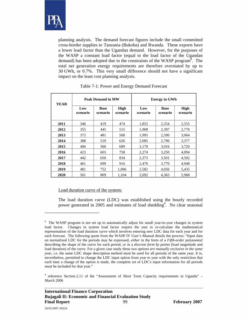
International Finance Corporation Bujagali II: Economic and Financial Evaluation Study Final Report 99 February 2007 26/02/2007-20224
planning analysis. The demand forecast figures include the small committed cross-border supplies to Tanzania (Bukoba) and Rwanda. These exports have a lower load factor than the Ugandan demand. However, for the purposes of the WASP a constant load factor (equal to the load factor of the Ugandan demand) has been adopted due to the constraints of the WASP program8. The total net generation energy requirements are therefore overstated by up to 30 GWh, or 0.7%. This very small difference should not have a significant impact on the least cost planning analysis.
Table 7-1: Power and Energy Demand Forecast
Peak Demand in MW Energy in GWh YEAR
Low scenario
Base scenario
High scenario
Low scenario
Base scenario
High scenario
2011 346 419 474 1,855 2,254 2,555 2012 355 445 515 1,908 2,397 2,776 2013 372 481 568 1,995 2,590 3,064 2014 388 519 626 2,085 2,796 3,377 2015 406 560 689 2,178 3,016 3,720 2016 423 603 758 2,274 3,250 4,094 2017 442 650 834 2,373 3,501 4,502 2018 461 699 916 2,476 3,770 4,948 2019 481 752 1,006 2,582 4,056 5,435 2020 501 809 1,104 2,692 4,363 5,968
Load duration curve of the system:
The load duration curve (LDC) was established using the hourly recorded power generated in 2005 and estimates of load shedding9. No clear seasonal
8 The WASP program is not set up to automatically adjust for small year-to-year changes in system load factor. Changes in system load factor require the user to re-calculate the mathematical representation of the load duration curve which involves entering new LDC data for each year and for each forecast. The following quote from the WASP IV User’s Manual details the process: “Input data on normalized LDC for the periods may be expressed, either in the form of a Fifth-order polynomial describing the shape of the curve for each period, or in a discrete form by points (load magnitude and load duration) of the curve. For a given case study these two options are mutually exclusive in the same year, i.e. the same LDC shape description method must be used for all periods of the same year. It is, nevertheless, permitted to change the LDC input option from year to year with the only restriction that each time a change of the option is made, the complete set of LDC's input information for all periods must be included for that year.”
9 reference Section 2.11 of the “Assessment of Short Term Capacity requirements in Uganda” – March 2006
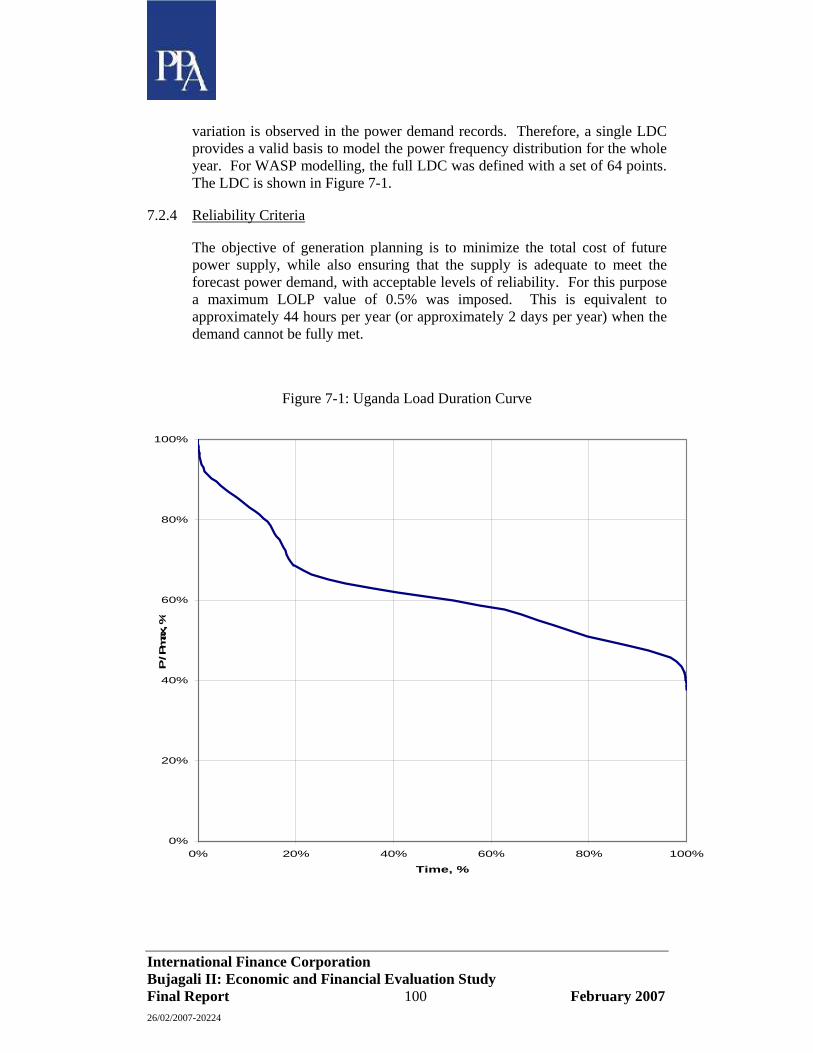
International Finance Corporation Bujagali II: Economic and Financial Evaluation Study Final Report 100 February 2007 26/02/2007-20224
variation is observed in the power demand records. Therefore, a single LDC provides a valid basis to model the power frequency distribution for the whole year. For WASP modelling, the full LDC was defined with a set of 64 points. The LDC is shown in Figure 7-1.
7.2.4 Reliability Criteria
The objective of generation planning is to minimize the total cost of future power supply, while also ensuring that the supply is adequate to meet the forecast power demand, with acceptable levels of reliability. For this purpose a maximum LOLP value of 0.5% was imposed. This is equivalent to approximately 44 hours per year (or approximately 2 days per year) when the demand cannot be fully met.
Figure 7-1: Uganda Load Duration Curve
0%
20%
40%
60%
80%
100%
0% 20% 40% 60% 80% 100%
Time, %
P / P
max
, %

International Finance Corporation Bujagali II: Economic and Financial Evaluation Study Final Report 101 February 2007 26/02/2007-20224
7.2.5 Economic Criteria
The following economic data were used in the calculations:
• Reference year for present-worth calculations is 2006. All capital costs of candidate thermal and hydro plants are estimated in 2006 money, and the earliest commissioning date considered is 2011. Therefore the effect of discounting all costs to 2006 would automatically generate a reduction factor with a maximum value of 1/1.15 = 0.62 on all capital costs.
• Discount rate: 10% is the test discount rate adopted for the studies, as directed by the World Bank Group.
7.2.6 Characteristics of Thermal Plants
Capital and O&M costs of Thermal Plants:
The capital costs of the candidate thermal power plants derive from the analysis in Section 5.1. Capital costs are summarized in Table 7-2 and Table 7-3. O&M costs calculations are based on the technical characteristics of the power plants and the fuels costs.
Fuel Costs:
Fuel costs are discussed in detail in Section 4.4. The World Bank’s mid-2006 forecast of international oil prices was used to estimate fuel prices in the future.
Table 7-4 shows the crude oil projections adopted and the corresponding calculated fuel costs in Uganda.
Generation Costs of Thermal Plants:
Preliminary screening analysis was carried out to determine the relative merits of the different thermal plants for base and peak load operation. These are presented in Section 5.1.
The WASP analysis allowed for the selection of any number of thermal plants as required by the optimising process, with the exception of the geothermal which was limited to a single unit of 40 MW as discussed in Section 5.2.

International Finance Corporation Bujagali II: Economic and Financial Evaluation Study Final Report 102 February 2007 26/02/2007-20224
Table 7-2: Capital Cost of Candidate Thermal Plants
Description UnitsGT
30MWGT
67MWCCGT
100MWLS Diesel
30MWLS Diesel
50MWMS Diesel
20MWOil Steam 100MW
Geothermal 40MW
Installed capacity MW 26 57 84 30 50 20 100 40Capital cost $'m 19.7 38.6 99.2 47.5 75.5 19.0 104.7 134.0Capital cost $/kW 758 678 1,180 1,584 1,510 951 1,047 3,350 - local $/kW 152 136 236 317 302 190 209 670 - foreign $/kW 607 542 944 1267 1208 761 838 2680Capital cost + IDC $/kW 859 768 1392 1830 1744 1099 1267 4055 - local $/kW 172 154 278 366 349 220 253 811 - foreign $/kW 688 614 1114 1464 1395 879 1014 3244Plant life Years 20 20 20 25 25 20 25 25Construction time Years 3 3 4 3 3 3 5 5Phasing of cost (% of capital cost)Year -4 5% 5%Year -3 15% 30% 30%Year -2 35% 35% 45% 55% 55% 55% 30% 30%Year -1 60% 60% 35% 40% 40% 40% 25% 25%Year 0 5% 5% 5% 5% 5% 5% 10% 10%IDC factors** 1.134 1.134 1.179 1.156 1.156 1.156 1.211 1.211Interest during construction (IDC) % of capital cost % 13.35 13.35 17.92 15.55 15.55 15.55 21.05 21.05
Economic Data for Candidate Plant
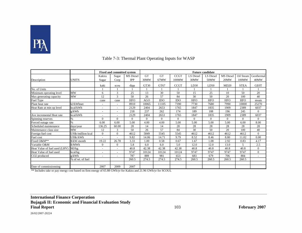
International Finance Corporation Bujagali II: Economic and Financial Evaluation Study Final Report 103 February 2007 26/02/2007-20224
Table 7-3: Thermal Plant Operating Inputs for WASP
Description UNITSKakira Sugar
Sugar Corp
MS Diesel IPP
GT 30MW
GT 67MW
CCGT 100MW
LS Diesel 30MW
LS Diesel 50MW
MS Diesel 20MW
Oil Steam 100MW
Geothermal 40MW
kaki scou dipp GT30 GT67 CCGT LD30 LD50 MD20 STEA GE0TNo. of Units 1 1 1 1 1 1 1 1 1 1 1Minimum operating level MW 6 3 25 13 30 50 15 25 10 50 20Max generating capacity MW 12 3 50 26 57 84 30 50 20 100 40Fuel Type cane cane HFO AGO IDO IDO HFO HFO HFO HFO steamPlant heat rate kJ/kWhnet - - 8910 10065 11105 7390 7730 7680 7990 10000 25270Heat Rate at min op level kcal/kWh - - 2129 2404 2653 1765 1847 1835 1909 2389 6037
g/kWh - - 218 237 262 174 189 188 196 245 0Ave incremental Heat rate kcal/kWh - - 2129 2404 2653 1765 1847 1835 1909 2389 6037Spinning reserves % 0 0 0 0 0 0 0 0 0 0 0Forced outage rate % 6.00 6.00 5.00 4.00 4.00 5.00 5.00 5.00 5.00 6.00 8.00Scheduled maintenance days/year 136.25 60.00 28 14 14 28 28 28 28 28 28Maintenance class size MW 12 3 50 26 57 84 30 50 20 100 40Foreign fuel cost US$c/million kcal 0 0 4612 5849 5545 5545 4612 4612 4612 4612 0Fuel cost US$c/kWh - - 9.82 14.06 14.71 9.79 8.52 8.46 8.80 11.02 0.00Fixed O&M** $/kW-month 19.22 26.78 3.33 1.00 0.58 0.67 1.67 1.08 2.92 0.83 4.17Variable O&M $/MWh 0 0 5.8 6.0 6.0 5.0 12.0 12.0 13.0 5 2.5Heat Value of fuel used (LHV) MJ/kg - - 40.8 42.38 42.38 42.38 40.8 40.8 40.8 40.8 0Heat Value of fuel used kcal/kg - - 9747 10124 10124 10124 9747 9747 9747 9747 0CO2 produced g/kWh - - 787 889 981 653 683 679 706 884 -
% of wt. of fuel 260.5 274.5 274.5 274.5 260.5 260.5 260.5 260.5
Date of commissionning 2007 2009 2007** Includes take or pay energy cost based on firm energy of 65.88 GWh/yr for Kakira and 21.96 GWh/yr for SCOUL
Fixed and committed system Future candidate
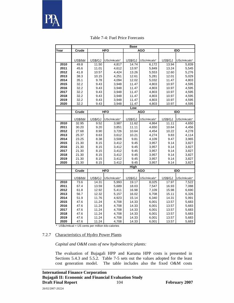
International Finance Corporation Bujagali II: Economic and Financial Evaluation Study Draft Final Report 104 February 2007 26/02/2007-20224
Table 7-4: Fuel Price Forecasts
Year Crude
US$/bbl US$/GJ USc/mkcals* US$/GJ USc/mkcals* US$/GJ USc/mkcals*2010 49.8 11.50 4,817 14.74 6,172 13.94 5,839 2011 45.6 11.01 4,612 13.97 5,849 13.24 5,545 2012 41.8 10.57 4,424 13.26 5,553 12.60 5,276 2013 38.3 10.15 4,251 12.61 5,281 12.01 5,029 2014 35.1 9.78 4,094 12.02 5,032 11.47 4,803 2015 32.2 9.43 3,948 11.47 4,803 10.97 4,595 2016 32.2 9.43 3,948 11.47 4,803 10.97 4,595 2017 32.2 9.43 3,948 11.47 4,803 10.97 4,595 2018 32.2 9.43 3,948 11.47 4,803 10.97 4,595 2019 32.2 9.43 3,948 11.47 4,803 10.97 4,595 2020 32.2 9.43 3,948 11.47 4,803 10.97 4,595
Crude
US$/bbl US$/GJ USc/mkcals* US$/GJ USc/mkcals* US$/GJ USc/mkcals*2010 32.95 9.52 3,987 11.62 4,864 11.11 4,650 2011 30.20 9.20 3,851 11.11 4,650 10.64 4,456 2012 27.68 8.90 3,726 10.64 4,454 10.22 4,278 2013 25.37 8.63 3,612 10.21 4,274 9.83 4,114 2014 23.25 8.38 3,508 9.81 4,109 9.47 3,965 2015 21.30 8.15 3,412 9.45 3,957 9.14 3,827 2016 21.30 8.15 3,412 9.45 3,957 9.14 3,827 2017 21.30 8.15 3,412 9.45 3,957 9.14 3,827 2018 21.30 8.15 3,412 9.45 3,957 9.14 3,827 2019 21.30 8.15 3,412 9.45 3,957 9.14 3,827 2020 21.30 8.15 3,412 9.45 3,957 9.14 3,827
Crude
US$/bbl US$/GJ USc/mkcals* US$/GJ USc/mkcals* US$/GJ USc/mkcals*2010 73.6 14.31 5,993 19.17 8,025 17.97 7,522 2011 67.4 13.59 5,689 18.03 7,547 16.93 7,088 2012 61.8 12.92 5,411 16.98 7,109 15.98 6,690 2013 56.7 12.32 5,157 16.02 6,708 15.11 6,326 2014 51.9 11.76 4,923 15.14 6,340 14.31 5,991 2015 47.6 11.24 4,708 14.33 6,001 13.57 5,683 2016 47.6 11.24 4,708 14.33 6,001 13.57 5,683 2017 47.6 11.24 4,708 14.33 6,001 13.57 5,683 2018 47.6 11.24 4,708 14.33 6,001 13.57 5,683 2019 47.6 11.24 4,708 14.33 6,001 13.57 5,683 2020 47.6 11.24 4,708 14.33 6,001 13.57 5,683
* US$c/mkcal = US cents per million kilo-calories
HFO
IDO
IDO
Base
Low
High
IDO
HFO AGO
HFO AGO
AGO
7.2.7 Characteristics of Hydro Power Plants
Capital and O&M costs of new hydroelectric plants:
The evaluation of Bujagali HPP and Karuma HPP costs is presented in Sections 5.4.3 and 5.5.2. Table 7-5 sets out the values adopted for the least cost generation model. The table includes also the fixed O&M costs

International Finance Corporation Bujagali II: Economic and Financial Evaluation Study Final Report 105 February 2007 26/02/2007-20224
calculated as the sum of 0.5% of the construction cost of civil works and 1% of the cost of electromechanical equipment.
The IDC is calculated at the 10% discount rate.
Table 7-5: Capital Costs and Main Economic Characteristics of Candidate Hydroelectric Plants
Item Data for Candidate Hydro Power Plants
Description Unit Bujagali 5 units Karuma Bujagali
4 units Installed capacity MW 250 200 200 Capital cost US$’m 520.6 587.8 491.3 Capital cost (without IDC) US$/kW 2082 2939 2457
domestic US$/kW 717 1127 873 foreign US$/kW 1365 1812 1583
Capital cost + IDC US$/kW 2606 3821 3075 domestic US$/kW 897 1465 1093
foreign US$/kW 1709 2356 1982 Plant life years 50 50 50 Construction time Year 4 5 4 IDC Amount, in % of Capital Cost % 25.15 30.00 25.17 O&M Cost US$/kW/month 1.00 1.14 1.14
Generation Characteristics of Hydro Power Plants:
The detailed analysis of the candidate plants is presented in Section 5. The power and energy generation of all candidate plants is presented in Section 3.
The main data on hydro power and energy required for the WASP modelling is summarised in Table 7-6. These characteristics are derived from reservoir operation studies, after due consideration of the impact of outages of generating units for maintenance. Details of calculations are presented in Appendix B - Hydrological Performance of Lake Victoria.

International Finance Corporation Bujagali II: Economic and Financial Evaluation Study Final Report 106 February 2007 26/02/2007-20224
Table 7-6: Summary of Energy and Power Characteristics of Major hydro power plant options
Bujagali 5 units
Bujagali 4 units
Karuma withoutBujagali
Karuma with
Bujagali
Na-Ki + Bu. 5 u.
Na-Ki + Bu 4 u.
Na-Ki + Karuma
A. LOW HYDROLOGY Emean * GWh/yr 1165 1171 1324 1338 2137 2143 2296Ebase GWh/yr 971 1064 1323 1337 1785 1949 2137Available Capacity MW 250 200 158 158 453 362 361B. HIGH HYDROLOGY Emean GWh/yr 1991 1601 1609 1620 3731 3341 3349Ebase GWh/yr 1989 1599 1607 1618 3729 3339 3347Available Capacity MW 250 200 200 200 454 404 404
* mean energy is equal to firm energy since there is no spill.
7.3 Power Generation Situation in 2011
The total available capacity in 2011, before adding any additional capacity, is assumed to be approximately 315 MW, with a small variation depending on the hydrological situation at the time. This total capacity essentially comprises Nalubaale – Kiira hydro power plant, small hydros, bio-mass plants and the medium speed diesel plant to be developed under an IPP arrangement. The capacities and commissioning date of these plants are shown in Table 7-7.
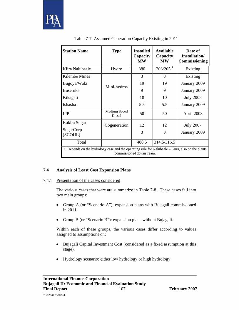
International Finance Corporation Bujagali II: Economic and Financial Evaluation Study Final Report 107 February 2007 26/02/2007-20224
Table 7-7: Assumed Generation Capacity Existing in 2011
Station Name Type Installed Capacity
MW
Available Capacity
MW
Date of Installation/
Commissioning
Kiira Nalubaale Hydro 380 203/205 1 Existing
Kilembe Mines Bugoye/Waki Buseruka Kikagati Ishasha
Mini-hydros
3 19 9 10 5.5
3 19 9 10 5.5
Existing January 2009 January 2009
July 2008 January 2009
IPP Medium Speed Diesel 50 50 April 2008
Kakira Sugar SugarCorp (SCOUL)
Cogeneration
12 3
12 3
July 2007 January 2009
Total 488.5 314.5/316.5 1. Depends on the hydrology case and the operating rule for Nalubaale – Kiira, also on the plants
commissioned downstream.
7.4 Analysis of Least Cost Expansion Plans
7.4.1 Presentation of the cases considered
The various cases that were are summarize in Table 7-8. These cases fall into two main groups:
• Group A (or “Scenario A”): expansion plans with Bujagali commissioned in 2011;
• Group B (or “Scenario B”): expansion plans without Bujagali.
Within each of these groups, the various cases differ according to values assigned to assumptions on:
• Bujagali Capital Investment Cost (considered as a fixed assumption at this stage),
• Hydrology scenario: either low hydrology or high hydrology

International Finance Corporation Bujagali II: Economic and Financial Evaluation Study Final Report 108 February 2007 26/02/2007-20224
• Non-Bujagali costs: limited to fuel costs of thermal plants, as these costs represent the most significant costs of alternative plants competing with Bujagali, with a wide range of possible variation in the medium to long term. Base, low and high fuel costs were defined. The base fuel cost forecast follows the latest World Bank forecast of crude oil prices, dated July 2006. At this stage of the evaluation, only the base case was considered. High and low fuel cost scenarios were developed, as discussed in Section 4.6, and presented in Table 7-4.
• Power and energy demand forecast: base, low and high scenarios were defined in Section 2 and are summarised in Table 7-1.
The complete risk analysis is presented in Section 7.5). It consists of the combination of the results obtained for the two hydrology scenarios (low and high), the three demand scenarios (base, low and high), the three fuel cost scenarios, and the three cost scenarios for Bujagali, each of these combinations considered with Bujagali and without Bujagali. This represents a total of 2x2x3x3 = 36 cases, which are shown in Table 7.8. In addition, the ‘with Bujagali’ cases are considered for high and low capital cost scenarios. This increases the number of ‘with Bujagali’ cases from 18 to 54, making 72 cases in all to be considered in the risk analysis.
A number of other cases had to be assessed in order to provide additional information for the least cost planning process with regard to the commissioning date and number of generating units for Bujagali, and an all thermal case. The results of these cases are shown in Table 7-9.
Detailed results of all WASP calculations are presented in Appendix E. The results are discussed in the following paragraphs, together with summary tables and figures.
7.4.2 Main Results and Conclusions of the Analysis
The results obtained by WASP for the main ‘with’ and without’ Bujagali cases calculations are presented in Table 7-8 below. The Net Present Value is shown as the difference between the present worth total cost of the expansion plan without Bujagali and the present worth total cost of the expansion plan with Bujagali, for any given set of assumptions that are equivalent except for the presence or absence of Bujagali, ‘Ref Case’ column indicates the case number of the corresponding case ‘without Bujagali’.
All PW values exclude credits for CO2 emissions. These are relatively small in the context of the total benefits of Bujagali, and Karuma, and have been considered in a separate sensitivity study in the EIRR analysis in Section 8.
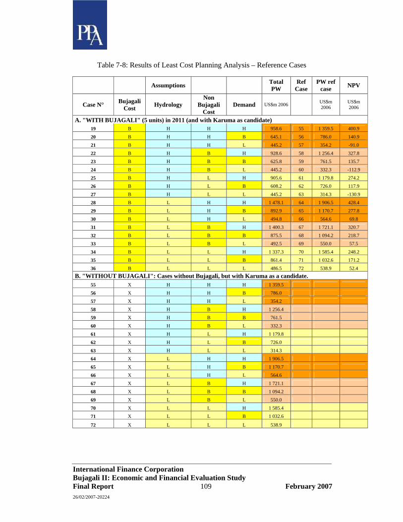
International Finance Corporation Bujagali II: Economic and Financial Evaluation Study Final Report 109 February 2007 26/02/2007-20224
Table 7-8: Results of Least Cost Planning Analysis – Reference Cases
Assumptions Total PW
Ref Case
PW ref case NPV
Case N° Bujagali Cost Hydrology
Non Bujagali
Cost Demand US$m 2006 US$m
2006 US$m 2006
A. "WITH BUJAGALI" (5 units) in 2011 (and with Karuma as candidate) 19 B H H H 958.6 55 1 359.5 400.9
20 B H H B 645.1 56 786.0 140.9
21 B H H L 445.2 57 354.2 -91.0
22 B H B H 928.6 58 1 256.4 327.8
23 B H B B 625.8 59 761.5 135.7
24 B H B L 445.2 60 332.3 -112.9
25 B H L H 905.6 61 1 179.8 274.2
26 B H L B 608.2 62 726.0 117.9
27 B H L L 445.2 63 314.3 -130.9
28 B L H H 1 478.1 64 1 906.5 428.4
29 B L H B 892.9 65 1 170.7 277.8
30 B L H L 494.8 66 564.6 69.8
31 B L B H 1 400.3 67 1 721.1 320.7
32 B L B B 875.5 68 1 094.2 218.7
33 B L B L 492.5 69 550.0 57.5
34 B L L H 1 337.3 70 1 585.4 248.2
35 B L L B 861.4 71 1 032.6 171.2
36 B L L L 486.5 72 538.9 52.4 B. "WITHOUT BUJAGALI": Cases without Bujagali, but with Karuma as a candidate.
55 X H H H 1 359.5
56 X H H B 786.0
57 X H H L 354.2
58 X H B H 1 256.4
59 X H B B 761.5
60 X H B L 332.3
61 X H L H 1 179.8
62 X H L B 726.0
63 X H L L 314.3
64 X L H H 1 906.5
65 X L H B 1 170.7
66 X L H L 564.6
67 X L B H 1 721.1
68 X L B B 1 094.2
69 X L B L 550.0
70 X L L H 1 585.4
71 X L L B 1 032.6
72 X L L L 538.9

International Finance Corporation Bujagali II: Economic and Financial Evaluation Study Final Report 110 February 2007 26/02/2007-20224
The results of other calculations for the assessment of the influence of varying key assumptions and modifications imposed on the plant sequencing are presented in Table 7-9. In this table, differences in PW costs are presented in the right hand column, after indicating the reference cases to which each new case is compared.
Table 7-9: Results of Least Cost Planning Analysis – Sensitivity Cases
Assumptions: Total PW
Ref Case
PW ref case NPV
Case N° Buj. Cost Hydrology Non Buj. Cost Demand US$m
2006 US$m 2006
US$m 2006
C-1. Other cases with Bujagali Bujagali 2012, construction 2008 – 2011
73 B L B B 924.9 32 875.5 -49.4 74 B H B B 606.5 23 625.8 19.3
Bujagali 2012, construction 2007 – 2011 73-B B L B B 946.2 32 875.5 -70.7 74-B B H B B 627.8 23 625.8 -2.0
Bujagali 4 units 77 B L B B 902.8 32 875.5 -27.3 78 B H B B 690.4 23 625.8 -64.6
Karuma imposed before Bujagali 79 B L B B 948.7 32 875.5 -73.2 80 B H B B 722.4 23 625.8 -96.6
C-2. Other cases without Bujagali Karuma forced in 2012:
59-F X H B B 783.8 60-F X H B L 467.6
Karuma in 2011 (theoretical) 68-B X L B B 1 042.2
Thermal least cost options (without Bujagali and Karuma) 81 X H B B 980.2 82 X L B B 1 361.0
These results produce the following key conclusions:
(i) The Net Present Value (NPV) of Bujagali HPP commissioned in 2011 is positive for both hydrology scenarios: it is US$ 219 million and US$ 136 million respectively for the low hydrology and the high hydrology under the base demand forecast. The NPV is higher for the low hydrology scenario since the energy capability of Bujagali is used up more quickly as compared to the high hydrology scenario, thus displacing more thermal, at an earlier date than would occur under the high hydrology scenario.

International Finance Corporation Bujagali II: Economic and Financial Evaluation Study Final Report 111 February 2007 26/02/2007-20224
(ii) Bujagali commissioning date delayed by one year (to 2012), yields a US$ 49 million increase in PW cost (and therefore a decrease of the NPV by the same amount) for the low hydrology, as compared to Bujagali commissioned in 2011. This is the earliest feasible commissioning date for Bujagali and the project should relieve the generating capacity shortage that is already being experienced in Uganda.
(iii) In most cases the least-cost expansion plans generated by WASP show Bujagali commissioning in 2011. The only exception is the high hydrology – low demand case, for which the power and energy generation from Nalubaale – Kiira is so high compared to the demand, that Bujagali is not selected before 2020. In these cases with high hydrology and low demand the capacity of the existing plant is sufficient to meet the demand until beyond 2020. The probability of occurrence of these cases is only about 6% (30% probability of low demand and 21% probability of high hydrology).
(iv) The least-cost expansion plan obtained for the low hydrology and base demand forecast is:
• Bujagali in 2011
• Geothermal (40 MW) in 2014
• Medium Speed Diesel (2x20 MW) in 2016
• Karuma 200 MW in 2017
• Gas Turbine (30 MW) in 2020
(v) The Net Present Value of Bujagali increases strongly when the demand increases and is relatively stable between low and high hydrology.
(vi) The case in which the commissioning of Karuma is imposed before Bujagali (Case 79) leads to an increase in PW cost of US$ 73 million for the low hydrology, and US$ 97 million for the high hydrology. The principal reason is the extra capital cost of Karuma compared to Bujagali for a similar energy output and a higher capacity at Bujagali.
(vii) The cases in which Bujagali with 4 units (200 MW) is commissioned in 2011 (Cases 77 & 78) show higher PW costs than the corresponding 5 unit cases (Cases 32 & 23): the differences are US$ 27 million for the low hydrology, and US$ 65 million for the high hydrology. Bujagali with 5 units is therefore economically more attractive than Bujagali with 4 units. (Note this decision is more robust than was the case for the evaluation of Bujagali I. This is due to the later commissioning date and the lower energy availability under the current low hydrology scenario).
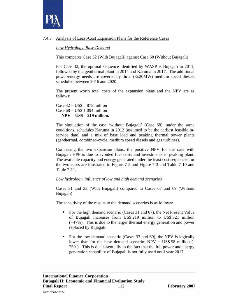
International Finance Corporation Bujagali II: Economic and Financial Evaluation Study Final Report 112 February 2007 26/02/2007-20224
7.4.3 Analysis of Least-Cost Expansion Plans for the Reference Cases
Low Hydrology, Base Demand
This compares Case 32 (With Bujagali) against Case 68 (Without Bujagali)
For Case 32, the optimal sequence identified by WASP is Bujagali in 2011, followed by the geothermal plant in 2014 and Karuma in 2017. The additional power/energy needs are covered by three (3x20MW) medium speed diesels scheduled between 2016 and 2020.
The present worth total costs of the expansion plans and the NPV are as follows:
Case 32 = US$ 875 million Case 68 = US$ 1 094 million NPV = US$ 219 million.
The simulation of the case ‘without Bujagali’ (Case 68), under the same conditions, schedules Karuma in 2012 (assumed to be the earliest feasible in-service date) and a mix of base load and peaking thermal power plants (geothermal, combined-cycle, medium speed diesels and gas turbines).
Comparing the two expansion plans, the positive NPV for the case with Bujagali HPP is due to avoided fuel costs and investments in peaking plant. The available capacity and energy generated under the least cost sequences for the two cases are illustrated in Figure 7-2 and Figure 7-3 and Table 7-10 and Table 7-11.
Low hydrology, influence of low and high demand scenarios
Cases 31 and 33 (With Bujagali) compared to Cases 67 and 69 (Without Bujagali)
The sensitivity of the results to the demand scenarios is as follows:
For the high demand scenario (Cases 31 and 67), the Net Present Value of Bujagali increases from US$ 219 million to US$ 321 million (+47%). This is due to the larger thermal energy generation and power replaced by Bujagali.
For the low demand scenario (Cases 33 and 69), the NPV is logically lower than for the base demand scenario: NPV = US$ 58 million (-75%). This is due essentially to the fact that the full power and energy generation capability of Bujagali is not fully used until year 2017.
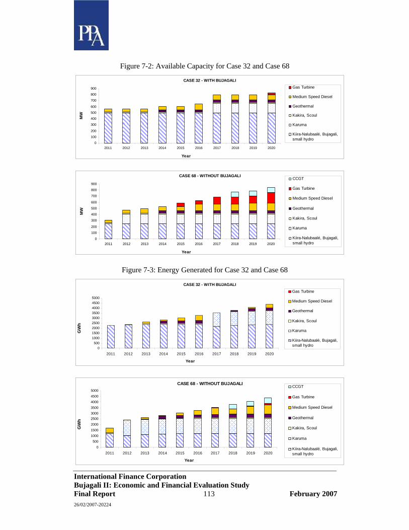
International Finance Corporation Bujagali II: Economic and Financial Evaluation Study Final Report 113 February 2007 26/02/2007-20224
Figure 7-2: Available Capacity for Case 32 and Case 68
CASE 32 - WITH BUJAGALI
0
100
200
300
400
500
600
700
800
900
2011 2012 2013 2014 2015 2016 2017 2018 2019 2020
MW
Gas Turbine
Medium Speed Diesel
Geothermal
Kakira, Scoul
Karuma
Kiira-Nalubaalé, Bujagali,small hydro
Year
CASE 68 - WITHOUT BUJAGALI
0
100
200
300
400
500
600
700
800
900
2011 2012 2013 2014 2015 2016 2017 2018 2019 2020
MW
CCGT
Gas Turbine
Medium Speed Diesel
Geothermal
Kakira, Scoul
Karuma
Kiira-Nalubaalé, Bujagali,small hydro
Year
Figure 7-3: Energy Generated for Case 32 and Case 68
CASE 32 - WITH BUJAGALI
0500
100015002000250030003500400045005000
2011 2012 2013 2014 2015 2016 2017 2018 2019 2020
Year
GW
h
Gas Turbine
Medium Speed Diesel
Geothermal
Kakira, Scoul
Karuma
Kiira-Nalubaalé, Bujagali,small hydro
CASE 68 - WITHOUT BUJAGALI
0500
100015002000250030003500400045005000
2011 2012 2013 2014 2015 2016 2017 2018 2019 2020
Year
GW
h
CCGT
Gas Turbine
Medium Speed Diesel
Geothermal
Kakira, Scoul
Karuma
Kiira-Nalubaalé, Bujagali,small hydro
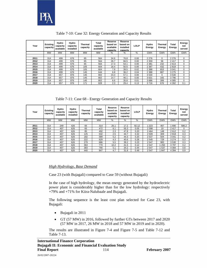
International Finance Corporation Bujagali II: Economic and Financial Evaluation Study Final Report 114 February 2007 26/02/2007-20224
Table 7-10: Case 32: Energy Generation and Capacity Results
Table 7-11: Case 68 - Energy Generation and Capacity Results
High Hydrology, Base Demand
Case 23 (with Bujagali) compared to Case 59 (without Bujagali)
In the case of high hydrology, the mean energy generated by the hydroelectric power plant is considerably higher than for the low hydrology: respectively +79% and +71% for Kiira-Nalubaale and Bujagali.
The following sequence is the least cost plan selected for Case 23, with Bujagali:
• Bujagali in 2011
• GT (57 MW) in 2016, followed by further GTs between 2017 and 2020 (57 MW in 2017, 26 MW in 2018 and 57 MW in 2019 and in 2020).
The results are illustrated in Figure 7-4 and Figure 7-5 and Table 7-12 and Table 7-13.
Year Existing capacity
Hydro capacity available
Hydro capacity installed
Thermal capacity
Total capacity available
Reserve based on available capacity
Reserve based on installed capacity
LOLP Hydro Energy
Thermal Energy
Total Energy
Energy not
served
MW MW MW MW MW % % % GWh GWh GWh GWh
2011 314 499 676 65 564 34.6 76.8 0.00 2 276 0 2 276 02012 314 499 676 65 564 26.7 66.5 0.00 2 359 58 2 417 02013 314 499 676 65 564 17.3 54.1 0.00 2 381 232 2 613 02014 314 499 676 105 604 16.4 50.5 0.00 2 387 432 2 819 02015 314 499 676 105 604 7.9 39.5 0.02 2 388 653 3 041 02016 314 499 676 145 644 6.8 36.2 0.04 2 388 887 3 275 02017 314 657 876 145 802 23.4 57.1 0.00 3 530 0 3 530 02018 314 657 876 145 802 14.7 46.1 0.00 3 631 165 3 796 02019 314 657 876 145 802 6.6 35.8 0.01 3 686 399 4 085 02020 314 657 876 171 828 2.3 29.4 0.13 3 716 676 4 392 0.1
Year Existing capacity
Hydro capacity available
Hydro capacity installed
Thermal capacity
Total capacity available
Reserve based on available capacity
Reserve based on installed capacity
LOLP Hydro Energy
Thermal Energy
Total Energy
Energy not
served
MW MW MW MW MW % % % GWh GWh GWh GWh
2011 314 249 426 65 314 25.1 - 17.2 92.12 1 223 467 1 690 586.22012 314 407 626 65 472 6.1 55.3 0.05 2 398 19 2 417 02013 314 407 626 85 492 2.3 47.8 0.20 2 464 148 2 612 0.22014 314 407 626 125 532 2.5 44.7 0.32 2 509 309 2 818 0.32015 314 407 626 182 589 5.2 44.3 0.20 2 537 504 3 041 0.22016 314 407 626 222 629 4.3 40.6 0.28 2 545 729 3 274 0.32017 314 407 626 279 686 5.5 39.2 0.23 2 547 983 3 530 0.32018 314 407 626 363 770 10.2 41.5 0.12 2 547 1 250 3 797 0.22019 314 407 626 383 790 5.1 34.2 0.44 2 547 1 537 4 084 0.82020 314 407 626 440 847 4.7 31.8 0.49 2 547 1 847 4 394 0.9
International Finance Corporation Bujagali II: Economic and Financial Evaluation Study Final Report 115 February 2007 26/02/2007-20224
Figure 7-4: Available Capacity for Case 23 and Case 59
The reason for the non–selection of Karuma in Case 23, is apparent in Figure 7-5, where one observes that the full energy generation provided by Nalubaale – Kiira and Bujagali is not fully consumed by the system before 2020. The requirement for new generation on the system before 2020 is therefore for capacity rather than energy, which can be provided most cost effectively by peaking gas turbine plant.
CASE 23 - WITH BUJAGALI
0
100
200
300
400
500
600
700
800
900
2011 2012 2013 2014 2015 2016 2017 2018 2019 2020
MW
Gas Turbine
Medium Speed Diesel
Geothermal
Kakira, Scoul
Karuma
Kiira-Nalubaalé, Bujagali,small hydro
Year
CASE 59 - WITHOUT BUJAGALI
0100200300400500600700800900
1 000
2011 2012 2013 2014 2015 2016 2017 2018 2019 2020
MW
Gas Turbine
Medium Speed Diesel
Geothermal
Kakira, Scoul
Karuma
Kiira-Nalubaalé, Bujagali,small hydro
Year
International Finance Corporation Bujagali II: Economic and Financial Evaluation Study Final Report 116 February 2007 26/02/2007-20224
Figure 7-5: Energy Generated for Case 23 and Case 59
Table 7-12: Case 23 - Energy Generation and Capacity Results
CASE 59 - WITHOUT BUJAGALI
0500
100015002000250030003500400045005000
2011 2012 2013 2014 2015 2016 2017 2018 2019 2020
Year
GW
h
Gas Turbine
Medium Speed Diesel
Geothermal
Kakira, Scoul
Karuma
Kiira-Nalubaalé, Bujagali,small hydro
CASE 23 - WITH BUJAGALI
0500
100015002000250030003500400045005000
2011 2012 2013 2014 2015 2016 2017 2018 2019 2020
Year
GW
h
Gas Turbine
Medium Speed Diesel
Geothermal
Kakira, Scoul
Karuma
Kiira-Nalubaalé, Bujagali, smallhydro
Year Existing capacity
Hydro capacity available
Hydro capacity installed
Thermal capacity
Total capacity available
Reserve based on available capacity
Reserve based on installed capacity
LOLP Hydro Energy
Thermal Energy
Total Energy
Energy not
served
MW MW MW MW MW % % % GWh GWh GWh GWh
2011 314 501 676 65 566 35.1 76.8 0.00 2 276 0 2 276 02012 314 501 676 65 566 27.2 66.5 0.00 2 417 0 2 417 02013 314 501 676 65 566 17.7 54.1 0.00 2 613 0 2 613 02014 314 501 676 65 566 9.1 42.8 0.01 2 819 0 2 819 02015 314 501 676 65 566 1.1 32.3 0.19 3 034 7 3 041 0.12016 314 501 676 122 623 3.3 32.3 0.14 3 218 57 3 275 0.12017 314 501 676 179 680 4.6 31.5 0.12 3 411 119 3 530 0.12018 314 501 676 205 706 1.0 26.0 0.42 3 597 199 3 796 0.62019 314 501 676 262 763 1.5 24.7 0.42 3 748 336 4 084 0.62020 314 501 676 319 820 1.4 23.0 0.49 3 848 546 4 394 0.8

International Finance Corporation Bujagali II: Economic and Financial Evaluation Study Final Report 117 February 2007 26/02/2007-20224
Table 7-13: Case 59: Energy Generation and Capacity Results
High hydrology, influence of demand scenarios
Cases 22 and 24 (with Bujagali) compared to Cases 58 and 60 (without Bujagali)
The sensitivity of the results to the high and low demand scenarios is as follows:
For the high demand scenario (Cases 22 and 58), the Net Present Value of Bujagali increases from US$ 136 million to US$ 328 million (+241%). This is due to the high thermal generation under the high demand scenario which is replaced by hydro energy generated at Bujagali, and is more rapidly fully consumed by the system demand than under the base demand scenario.
For the low demand scenario (Cases 24 and 60), the NPV is negative, because the least cost plan is the plan without any additional hydro plant until at least 2020. The total generation capability of Nalubaale – Kiira and small hydro plants is effectively 2388 GWh/year (see Table 7-6), while the total energy demand in 2020 is only 2721 GWh in the low demand scenario. The low additional energy to be generated to meet the demand is most economically supplied by thermal plants (MD20 starting in 2013, and GT67 starting in 2014). In this case, Bujagali commissioning in 2011 had to be imposed on the WASP program, so that the risk analysis could be performed on NPVs calculated on the same basis, that is to say Bujagali commissioning in 2011.
7.4.4 Analysis of Least-Cost Expansion Plans for sensitivity cases
The results of the sensitivity cases are presented in Table 7-9.
Year Existing capacity
Hydro capacity available
Hydro capacity installed
Thermal capacity
Total capacity available
Reserve based on available capacity
Reserve based on installed capacity
LOLP Hydro Energy
Thermal Energy
Total Energy
Energy not
served
MW MW MW MW MW % % % GWh GWh GWh GWh
2011 314 251 426 65 316 24.6 - 17.2 20.89 1 947 233 2 180 95.82012 314 451 626 65 516 16.0 55.3 0.00 2 417 0 2 417 02013 314 451 626 65 516 7.3 43.7 0.02 2 605 8 2 613 02014 314 451 626 85 536 3.3 37.0 0.18 2 780 39 2 819 0.12015 314 451 626 142 593 5.9 37.1 0.08 2 949 93 3 042 0.12016 314 451 626 199 650 7.8 36.8 0.07 3 114 161 3 275 0.12017 314 451 626 256 707 8.8 35.7 0.06 3 253 277 3 530 02018 314 451 626 296 747 6.9 31.9 0.13 3 341 455 3 796 0.22019 314 451 626 353 804 6.9 30.2 0.15 3 405 680 4 085 0.22020 314 451 626 410 861 6.4 28.1 0.18 3 445 949 4 394 0.2
International Finance Corporation Bujagali II: Economic and Financial Evaluation Study Final Report 118 February 2007 26/02/2007-20224
Bujagali commissioning postponed to 2012 (4 years construction 2008-2011)
This sensitivity analysis is covered by Cases 73 and 74 (low and high hydrology respectively) compared to Cases 32 and 23 which are the corresponding “with Bujagali commissioned in 2011” cases.
For the low hydrology situation (Case 73 compared to Case 32), the consequence of postponing commissioning of Bujagali by one year is a decrease of the NPV by US$ 49 million (or an increase of PW total cost by the same amount). This results from the high cost of the energy that would be expended in 2011 to replace the generation of Bujagali. The cost of generating this energy in 2011 is much higher than the saving obtained by the postponement of the capital investment cost of Bujagali by one year. The additional thermal cost (valued at the marginal generation cost of leased high-speed diesel plant) remains lower than the economic cost of the 586 GWh unserved energy that would otherwise be incurred, if no additional means of generation were to be mobilised to compensate for the absence of Bujagali generation in 2011.
For the high hydrology situation (Case 74 compared to Case 23), the consequence of delaying the commissioning of Bujagali is quite different, as there is much more generation from Nalubaale – Kiira and only 96 GWh to be produced by additional thermal plant in 2011. The result is that the saving produced by the postponement of Bujagali investment is higher than the cost of replacement diesel generation required in 2011, and the total PW cost is decreased by US$ 19 million.
Given the probability of occurrence of low and high hydrology situations, and the relative costs of postponing the commissioning of Bujagali by one year, these sensitivity cases confirm that Bujagali commissioned in 2011 is economically more attractive than with Bujagali in 2012.
Bujagali commissioning postponed to 2012 (5 years construction: 2007-2011)
This sensitivity analysis is covered by Cases 73-B and 74-B (low and high hydrology respectively) compared to Cases 32 and 23 which are the corresponding “with Bujagali commissioned in 2011” cases.
The consequence of increasing the duration of construction by one year, and thus postponing commissioning of Bujagali by one year, is an increase in PW cost of US$ 71 million for the low hydrology, and US$ 2 million for the high hydrology. The principal reason of these results is the significant loss due to the loss of benefits from Bujagali energy in 2011 for the low hydrology. As regards the high hydrology scenario, the PW cost is hardly affected by the delay in construction time, because of the very low contribution of Bujagali in

International Finance Corporation Bujagali II: Economic and Financial Evaluation Study Final Report 119 February 2007 26/02/2007-20224
201129 , as Nalubaale –Kiira and small hydros will be able to meet almost the whole demand in 2011.
Bujagali equipped with 4 units:
This sensitivity analysis is covered by Cases 77 and 78 (low and high hydrology respectively) compared to Cases 32 and 23
For the low hydrology situation (Cases 77 and 32), the expansion plan with four units at Bujagali has the geothermal plant commissioned one year earlier (2013 rather than 2014) than in the 5-unit case (Case 32) and two gas turbines with a total capacity of 83 MW are included in 2015 and 2016 to compensate for the decrease in peaking capacity. The result is that the NPV is decreased by US$ 27 million, which confirms that the Bujagali with 5 units is superior to the 4-unit case, due principally to the additional peaking capacity it provides.
For the high hydrology (Cases 78 and 23), the decrease in NPV is US$ 65 million. This larger difference is due to the difference of over 400 GWh in the mean generation between the two options, which further penalizes the option with 4 units.
The conclusion of this sensitivity analysis is a clear economic advantage in favour of adopting 5 units at Bujagali.
Karuma imposed before Bujagali
This sensitivity analysis is covered by Cases 79 and 80 (low and high hydrology respectively) compared to Cases 32 and 23.
For both the low and high hydrology situations, the PW cost is found to be increased, by US$ 73 million and US$ 97 million respectively. The purpose of these cases was to quantify the economic advantage of commissioning Bujagali before Karuma.
Karuma imposed in 2011, without Bujagali
This sensitivity analysis is covered by Case 68-B (low hydrology) compared to Case 68 with Karuma in 2012. .
This case was performed to evaluate the difference in PW cost that would be obtained in the theoretical case when Karuma could be commissioned in 2011, although this is believed not to be feasible due to the less advanced stage of
29 These calculations do not take into account the benefits incurred by the improvement in the lake operation, when Bujagali is commissioned.

International Finance Corporation Bujagali II: Economic and Financial Evaluation Study Final Report 120 February 2007 26/02/2007-20224
development of Karuma, as compared to Bujagali, and also the nature of the civil works at Karuma which involve long tunnels and an underground power house. The PW cost of this expansion plan would be lower than Case 68 (with Karuma commissioned in 2012) by US$ 52 million. However, the Case 68-B with Karuma in 2011 still has a PW which is US$ 167 million higher than the comparative case with Bujagali in 2011 (Case 32).
Expansion Plan with neither Karuma nor Bujagali
This sensitivity analysis is covered by Cases 81 and 82 (high and low hydrology respectively). These cases were run for reference purposes, to evaluate the PW cost of the least-cost expansion plans based entirely on new thermal plant (including geothermal). The results are as follows:
In the low hydrology case (Case 82), the PW total cost is US$ 486 million (1361 – 875) higher than the least cost expansion plan with Bujagali and Karuma (Case 32), and US$ 267 million (1361 – 1094) higher than the least cost expansion plan without Bujagali but with Karuma (Case 68).
In the high hydrology case (Case 81), the PW total cost is US$ 354 million (980 – 626) higher than the least cost ‘with Bujagali’ expansion plan (Case 23), and US$ 218 million (980 – 762) higher than the ‘without Bujagali’ least cost expansion plan (Case 59) which includes Karuma.
Increase in Bujagali capital cost until Karuma becomes a better choice
WASP calculations were repeated for Case 32 (low hydrology, base demand, base fuel prices) with an increasing capital cost of Bujagali, to determine the magnitude of the increase for which the least cost expansion plan would no longer select Bujagali as the next best option for the expansion of the Ugandan system.
The result of this series of calculations is that Karuma becomes the favour option as the next major plant to be constructed when the increase in capital cost of Bujagali is 49% of the base cost estimate. The probability of such a large increase in the capital cost of Bujagali (while Karuma’s capital cost remains unchanged) is considered to be very small.
7.5 Risk Analysis
A risk analysis has been made to determine the impact on the least cost development plans with Bujagali of variations in key parameters. A decision tree analysis approach has been adopted.

International Finance Corporation Bujagali II: Economic and Financial Evaluation Study Final Report 121 February 2007 26/02/2007-20224
The analysis tests the robustness of the least cost plans with Bujagali to changes in the following key variables underlying the analysis:
Demand forecast: the base, high and low demand forecasts were assigned probabilities of 60%, 20% and 20% respectively. It was considered reasonable to assign a higher probability to the base forecast, since this is founded on the collective ‘most likely’ economic growth and loss parameters. The occurrence of the high and low forecasts is considered be equally likely and they are therefore assigned equal probability values.
Hydrology: the low and high release hydrology scenarios developed in this study are estimated to have probabilities of 79% and 21% respectively. The analysis on which these probability values were determined is set out in Section 3.2.
Fuel cost: the cost of the thermal plant is dominated by the cost of fuel. The sensitivity of the least cost plans to the high and low fuel cost projections is considered, based on the projections shown in Table 7-4. The high and low fuel costs are assigned probabilities of 30% each and the base fuel cost 40% probability.
Capital cost of Bujagali, including E&S costs: a range of -5% and +10% has been adopted for the risk analysis as discussed in Section 5.4.4. The probabilities assigned are 60% for the base cost and 20% each for the high and low cost estimates. The relatively high probability assigned to the base cost estimate takes cognisance of the advanced stage of development of the Bujagali project and the fact that the EPC contract has already been tendered and is in the final stages of negotiation. Equal probabilities are assigned to the high and low costs variations since each is considered equally likely given that the estimates assumed a skewed variation in the costs about the base value.
The risk analysis uses the PW values for the relevant cases with Bujagali and without Bujagali – there are 54 with Bujagali cases (3x18) to cover the full combination of sensitivities to be tested, as detailed above, plus 18 cases without Bujagali. Details of the full risk analysis matrix and the results are shown in Table 7-14.
The present worth (PW) values from the WASP least cost analysis for each case are inserted in the matrix table, together with their respective probability values. The PW values are then weighted with their respective probabilities. The resulting contributions from each branch of the decision tree are then summated to determine the probability weighted PW of the with and without Bujagali cases. The total without Bujagali is then subtracted from the total with Bujagali to obtain the total net present value (NPV).
International Finance Corporation Bujagali II: Economic and Financial Evaluation Study Final Report 122 February 2007 26/02/2007-20224
Assigning the probability weightings to the PW costs resulted in a total NPV advantage of US$ 184.0 million (in 2006 US$ with discounting to 2006) in favour of the ‘with Bujagali’ cases. The NPV value is robust in respect of the assumption on hydrology. For example, if 100% probability is assigned to either the low or the high hydrology scenarios, the NPVs, representing the differences between the ‘with Bujagali’ and ‘without Bujagali’ programmes, are:
Low hydrology US$ 202 million, and
High hydrology US$ 116 million
in favour of the ‘with Bujagali’ cases.

International Finance Corporation Bujagali II: Economic and Financial Evaluation Study Final Report 123 February 2007 26/02/2007-20224
Table 7-14: Risk Analysis for Bujagali Least Cost Programmes
PW Cost Prob. Weighted
Case # BUJ cost Hydrology Fuel cost Demand BUJ cost Hydrology Fuel cost Demand Weight US$m PW cost US$m
1 H H H H 0.2 0.21 0.3 0.30 0.004 997.2 3.82 H H H B 0.2 0.21 0.3 0.40 0.005 683.8 3.43 H H H L 0.2 0.21 0.3 0.30 0.004 483.8 1.84 H H B H 0.2 0.21 0.4 0.30 0.005 967.2 4.95 H H B B 0.2 0.21 0.4 0.40 0.007 664.4 4.56 H H B L 0.2 0.21 0.4 0.30 0.005 483.8 2.47 H H L H 0.2 0.21 0.3 0.30 0.004 944.3 3.68 H H L B 0.2 0.21 0.3 0.40 0.005 646.8 3.39 H H L L 0.2 0.21 0.3 0.30 0.004 483.8 1.8
10 H L H H 0.2 0.79 0.3 0.30 0.014 1516.8 21.611 H L H B 0.2 0.79 0.3 0.40 0.019 931.5 17.712 H L H L 0.2 0.79 0.3 0.30 0.014 533.5 7.613 H L B H 0.2 0.79 0.4 0.30 0.019 1439.0 27.314 H L B B 0.2 0.79 0.4 0.40 0.025 914.2 23.115 H L B L 0.2 0.79 0.4 0.30 0.019 531.1 10.116 H L L H 0.2 0.79 0.3 0.30 0.014 1375.9 19.617 H L L B 0.2 0.79 0.3 0.40 0.019 900.0 17.118 H L L L 0.2 0.79 0.3 0.30 0.014 525.2 7.519 B H H H 0.6 0.21 0.3 0.30 0.011 958.6 10.920 B H H B 0.6 0.21 0.3 0.40 0.015 645.1 9.821 B H H L 0.6 0.21 0.3 0.30 0.011 445.2 5.022 B H B H 0.6 0.21 0.4 0.30 0.015 928.6 14.023 B H B B 0.6 0.21 0.4 0.40 0.020 625.8 12.624 B H B L 0.6 0.21 0.4 0.30 0.015 445.2 6.725 B H L H 0.6 0.21 0.3 0.30 0.011 905.6 10.326 B H L B 0.6 0.21 0.3 0.40 0.015 608.2 9.227 B H L L 0.6 0.21 0.3 0.30 0.011 445.2 5.028 B L H H 0.6 0.79 0.3 0.30 0.043 1478.1 63.129 B L H B 0.6 0.79 0.3 0.40 0.057 892.9 50.830 B L H L 0.6 0.79 0.3 0.30 0.043 494.8 21.131 B L B H 0.6 0.79 0.4 0.30 0.057 1400.3 79.732 B L B B 0.6 0.79 0.4 0.40 0.076 875.5 66.433 B L B L 0.6 0.79 0.4 0.30 0.057 492.5 28.034 B L L H 0.6 0.79 0.3 0.30 0.043 1337.3 57.035 B L L B 0.6 0.79 0.3 0.40 0.057 861.4 49.036 B L L L 0.6 0.79 0.3 0.30 0.043 486.5 20.837 L H H H 0.2 0.21 0.3 0.30 0.004 939.3 3.638 L H H B 0.2 0.21 0.3 0.40 0.005 625.9 3.239 L H H L 0.2 0.21 0.3 0.30 0.004 425.9 1.640 L H B H 0.2 0.21 0.4 0.30 0.005 909.3 4.641 L H B B 0.2 0.21 0.4 0.40 0.007 606.5 4.142 L H B L 0.2 0.21 0.4 0.30 0.005 425.9 2.143 L H L H 0.2 0.21 0.3 0.30 0.004 886.4 3.444 L H L B 0.2 0.21 0.3 0.40 0.005 588.9 3.045 L H L L 0.2 0.21 0.3 0.30 0.004 425.9 1.646 L L H H 0.2 0.79 0.3 0.30 0.014 1458.9 20.747 L L H B 0.2 0.79 0.3 0.40 0.019 873.6 16.648 L L H L 0.2 0.79 0.3 0.30 0.014 475.6 6.849 L L B H 0.2 0.79 0.4 0.30 0.019 1381.1 26.250 L L B B 0.2 0.79 0.4 0.40 0.025 856.3 21.651 L L B L 0.2 0.79 0.4 0.30 0.019 473.2 9.052 L L L H 0.2 0.79 0.3 0.30 0.014 1318.0 18.753 L L L B 0.2 0.79 0.3 0.40 0.019 842.1 16.054 L L L L 0.2 0.79 0.3 0.30 0.014 467.3 6.6
1.000 869.5
With Bujagali in 2011 Probabilities of Occurrence

International Finance Corporation Bujagali II: Economic and Financial Evaluation Study Final Report 124 February 2007 26/02/2007-20224
55 H H H 0.21 0.3 0.30 0.019 1359.5 25.756 H H B 0.21 0.3 0.40 0.025 786.0 19.857 H H L 0.21 0.3 0.30 0.019 354.2 6.758 H B H 0.21 0.4 0.30 0.025 1256.4 31.759 H B B 0.21 0.4 0.40 0.034 761.5 25.660 H B L 0.21 0.4 0.30 0.025 332.3 8.461 H L H 0.21 0.3 0.30 0.019 1179.8 22.362 H L B 0.21 0.3 0.40 0.025 726.0 18.363 H L L 0.21 0.3 0.30 0.019 314.3 5.964 L H H 0.79 0.3 0.30 0.071 1906.5 135.665 L H B 0.79 0.3 0.40 0.095 1170.7 111.066 L H L 0.79 0.3 0.30 0.071 564.6 40.167 L B H 0.79 0.4 0.30 0.095 1721.1 163.268 L B B 0.79 0.4 0.40 0.126 1094.2 138.369 L B L 0.79 0.4 0.30 0.095 550.0 52.170 L L H 0.79 0.3 0.30 0.071 1585.4 112.771 L L B 0.79 0.3 0.40 0.095 1032.6 97.972 L L L 0.79 0.3 0.30 0.071 538.9 38.3
1.000 1053.6
NPV advantage of Bujagali US$m 184.0
Non-Bujagali Least Cost Option

International Finance Corporation Bujagali II: Economic and Financial Evaluation Study Final Report 125 February 2007 26/02/2007-20224
8 Economic Rate of Return
8.1 Methodology
In Section 7, above, least-cost generation expansion sequences for the Ugandan power sector were developed. The aim of this section of the report is to determine the economic internal rate of return (EIRR) of the Bujagali project.
The EIRR analysis is based on Case 23, for High hydrology and Case 32, for Low hydrology. In both cases, Bujagali is commissioned in 2011. The cases include base demand forecast, base Bujagali cost and base fuel price projections.
In addition to establishing the EIRR of the Bujagali project, this section covers a risk analysis on the key risk factors impacting on the project economics.
8.2 Assumptions
8.2.1 Baseline Assumptions for Incremental Costs and Demand
All discounting in the EIRR modelling is to a base year of 2006. Costs and benefits specific to the Bujagali project are captured for the period to end-2020, from studies detailed elsewhere in this report. Beyond 2020, a 40-year run-out period is adopted, with incremental costs and benefits held at the 2020 levels.
The baselines for individual line items in the analysis are not necessarily the same. Bujagali is assumed to commence operations at the beginning of 2011, and capital costs are assumed to commence in 2006.
Transmission investment costs, relating to incremental system expansion to absorb Bujagali output, are assumed to commence in 2010, i.e. 1 year before the actual demand increment commences.
Distribution investment costs, relating to incremental system expansion to absorb Bujagali output from 2011, are assumed to commence in 2011. The lead time on such construction is considered sufficiently short that investment and demand increments are assumed to coincide.
Generation, transmission and distribution operating costs are assumed to commence in 2011, with the commissioning of Bujagali.
The benefit stream is assumed to commence in 2011, with the commissioning of Bujagali.

International Finance Corporation Bujagali II: Economic and Financial Evaluation Study Final Report 126 February 2007 26/02/2007-20224
8.2.2 System Expansion Costs
The economic analysis is conducted solely with costs and benefits relating to the 250 MW Bujagali project. The analysis also takes into consideration the wider incremental costs associated with transmission and distribution infrastructure required to absorb Bujagali energy production into the system.
The total capital cost of the 250 MW Bujagali project, including engineering costs and social and environmental costs, but excluding interest during construction, is US$ 520.6 million. These costs are phased over the period 2007 to 2011, as discussed in Section 7 of the report.
An incremental transmission infrastructure cost of US$ 206.2/kW was determined by undertaking a long-run average incremental cost analysis on the Umeme transmission expansion plan. The phasing of the 250 MW demand increments was established, and the incremental cost was applied to the respective annual demand increments. Construction investments are assumed to precede demand increments by one year.
An incremental distribution infrastructure cost of US$ 1046.1 per new residential customer was determined by undertaking a long-run average incremental cost analysis on the Umeme distribution expansion plan. Although investment in distribution infrastructure is required for system reinforcement, as well as system extension purposes, expressing the cost in terms of new customer numbers is considered the most appropriate mechanism for undertaking the phasing. The phasing of the 250 MW demand increments was established, and the incremental cost was applied to the respective annual customer number increments. Distribution infrastructure investments are assumed to coincide with demand increments, i.e. with no significant lag between the investment and the demand growth being met by the new infrastructure.
The O&M cost of Bujagali was earlier determined as 1.00 US$/kW/month, which equates to US$ 3.0 million per year. Transmission O&M costs were assumed to be 1.0% of the cumulative transmission capacity cost increments, and distribution O&M costs were similarly assumed to be 2.0% of cumulative increments.
8.2.3 Reduction in Greenhouse Gas Emissions
To the extent that the commissioning of hydropower generation capacity displaces fossil-fuelled thermal capacity, there will be a commensurate reduction in the emission of greenhouse gases (GHGs). Since there is a basis for assigning monetary value to these emissions – measured in terms of equivalent tonnes of carbon dioxide (CO2) – it is possible to incorporate this in the economic analysis.

International Finance Corporation Bujagali II: Economic and Financial Evaluation Study Final Report 127 February 2007 26/02/2007-20224
The least-cost expansion sequence that includes Bujagali commissioned in 2011, will generate fewer GHG emissions than the least-cost sequence that does not include Bujagali. This notional reduction in emissions can be treated as a negative cost to the ‘with’ Bujagali expansion sequence, i.e. treated as such it becomes a benefit to this sequence. Since methane is a potent GHG, any methane generated by the Bujagali reservoir needs to be netted from the savings of CO2. These savings in CO2 are determined by evaluating the CO2 emission tonnages in the ‘with’ and ‘without’ Bujagali expansion sequences, using the WASP simulations.
The value of equivalent CO2 is obtained from the recent Stern Review, in which a minimum value of 25 US$/tonne of CO2 is proposed.30
In economic analysis, as opposed to financial analysis, the benefit of the ‘with’ Bujagali sequence over the ‘without’ Bujagali sequence is included because the impact on the environment takes place regardless of whether there is an actual market for the CO2 emission reductions.
8.2.4 Incremental Demand
Incremental demand is assessed for four customer groups, as follows:
• Newly-connected residential customers;
• Existing residential customers;
• Non-residential customers; and
• Exports.
The increments of demand in each year are driven by the increments of sales and exports, from the demand forecast. These sales increments are factored for system losses, to bring them to the generation level. An adjustment is made to take account of any unserved energy in 2010. The incremental demand is capped at the level achieved in the year at which the full energy production capability of Bujagali is absorbed by the system.
Incremental demand is valued using the commensurate willingness-to-pay value, the determination of which is outlined in Section 8.3, below, and is covered in greater detail in Appendix E.
30 “Stern Review: The Economics of Climate Change”, HM Treasury/Cabinet Office, UK, 2006.
International Finance Corporation Bujagali II: Economic and Financial Evaluation Study Final Report 128 February 2007 26/02/2007-20224
8.2.5 Residual Displaced Thermal Energy
A further benefit stream takes account of the thermal energy that is displaced by the introduction of Bujagali in 2011. Physically, these are likely to be the leased high-speed diesel units to be supplied under IDA funding, together with the HFO-fuelled medium-speed diesel units currently under procurement. The incremental energy equates to the difference between the 2010 and 2011 levels of output by these units, but the benefit is curtailed as the full energy production capability of Bujagali is absorbed by the system. The 2010 thermal energy production is obtained from analysis undertaken as part of a recent study of short-term thermal energy in Uganda, for the World Bank, whereas the 2011 thermal energy production is taken from the least-cost analysis using WASP. The mechanism applied is that once the sum of incremental demand and the initial level of displaced thermal energy would exceed the project’s energy capability, each year’s incremental demand replaces thermal displacement energy until the latter is extinguished.
Since this energy cannot be considered as catering to new demand until the capacity of the plant is consumed by load growth, the value is based on the weighted average of the displaced fuel and variable O&M cost and, in the case of the leased units, a proportion of the leasing cost. Fuel consumption is based on heat rates of 9902 and 8910 kJ/kWh for the high-speed and medium-speed units, respectively and the fuel cost is calculated for each year, in response to fuel price projections. Variable O&M costs are assumed to be 0.00952 and 0.0058 US$/kWh for the high-speed and medium-speed units, respectively.
As the residual thermal energy reduces, consistent with the absorption of Bujagali energy into the system, it is assumed that the high-speed diesel generated energy is removed first, since these units have higher marginal cost. The weighted-average value of the energy thus changes in each year.
8.2.6 Unserved Energy Cost
To the extent that unconstrained energy demand is not met, in any year, this constitutes a cost to the sequence. The values of expected unserved energy in each year, in GWh, are taken from the WASP modelling. The actual cost of unserved energy (CUE), in US$/kWh, is calculated for each year in the sequence, and the methodology is detailed in Appendix E.5.
The approach is to take the weighted-average CUE of residential and non-residential CUE values, with the weighting undertaken on the basis of the imputed split of unserved demand in 2005. For residential customers, the willingness-to-pay of newly-connected customers is estimated, in each year, by fitting an income-compensated demand curve between two points on the curve; the average tariff and average consumption are used to establish one point on the curve, and the cost and energy quantum of a representative mix of
International Finance Corporation Bujagali II: Economic and Financial Evaluation Study Final Report 129 February 2007 26/02/2007-20224
electricity substitutes are used to establish the other point. For non-residential customers, CUE is based on the cost of auxiliary generation.
8.3 Benefit Assumptions
8.3.1 Household Willingness-to-Pay
In estimating the economic benefits associated with incremental consumption by residential customers, the analysis differentiates between ‘existing’ and ‘new’ residential customers, where ‘new’ customers are defined as those that have been connected to the grid for less than one year. Benefits are based on principles of ‘willingness-to-pay’ (WTP). Details of the estimation of new residential customers is provided in Appendix E.1, whereas details for existing customers is provided in Appendix E.2.
Broadly, the value of incremental consumption by newly-connected residential customers is obtained by estimating the income-compensated demand curve for a cross-section of new electricity users, and measuring the value of the substitution effect of electricity supply plus the value of the incremental demand induced by having access to lower-cost electricity. Since the cost of some electricity substitutes are linked to the price of fuels and, ultimately, to the international price of crude oil, which is projected to move significantly, the WTP is estimated for all years in the planning horizon and linked to the crude oil price projections.
The willingness-to-pay for incremental consumption by existing residential customers is valued at the marginal tariff for this customer group. Since tariffs are projected to fluctuate in real terms, rising with the introduction of thermal capacity in the short-term and falling as a result of the commissioning of Bujagali, these real tariff changes are factored into the WTP projections for existing customers.
8.3.2 Industrial and Commercial Willingness-to-Pay
The detailed estimation of WTP by industrial and commercial customers is presented in Appendix E.3. The methodology is similar to that for newly-connected residential customers, and focuses on the cost of auxiliary generation. Once again, the avoided cost of auto-generation, and hence the WTP of industrial/commercial customers, is linked to the real price of crude oil on international markets.
8.3.3 Export Willingness-to-Pay
The willingness of export customers to pay for exports of secondary energy is assumed to be equivalent to the avoided cost of fuel in Tanzania and Rwanda. Details of the WTP calculation are presented in Appendix E.4. The WTP calculation is based on AGO-fuelled high-speed diesel units at Bukoba, in
International Finance Corporation Bujagali II: Economic and Financial Evaluation Study Final Report 130 February 2007 26/02/2007-20224
western Tanzania. The avoided cost in 2005 is estimated to be US$ 0.188 per kWh, and the value is calculated for each year, using fuel price projections.
8.4 Expected EIRR
8.4.1 General
Four EIRR determinations are presented in this sub-section. In each, the Base case demand scenario, the Base case fuel price scenario and the Base case Bujagali capital cost are adopted. Two scenarios use the High hydrology, and the other two use the Low hydrology. For each hydrology case, EIRR values are determined both ‘with’ and ‘without’ the greenhouse gas emissions cost stream.
8.4.2 High Hydrology
In the High hydrology scenario, the EIRR of the Bujagali project is 22.0%, ‘with’ greenhouse gas emissions costs, and 21.7% ‘without’. The discounted cash flow (DCF) calculations are summarised in Table 8-1 and Table 8-2.
8.4.3 Low Hydrology
In the Low hydrology scenario, the EIRR of the Bujagali project is 22.9%, ‘with’ greenhouse gas emissions costs, and 22.0% ‘without’. The discounted cash flow (DCF) calculations are summarised in Table 8-3 and Table 8-4
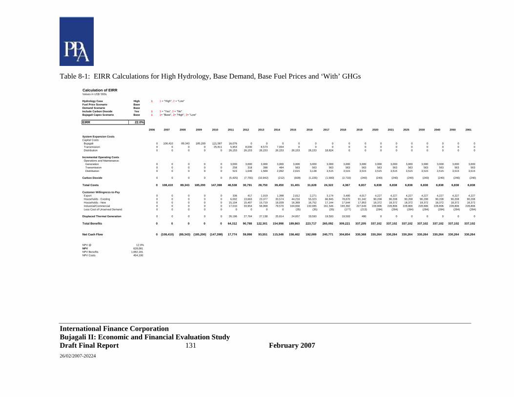
International Finance Corporation Bujagali II: Economic and Financial Evaluation Study Draft Final Report 131 February 2007 26/02/2007-20224
Table 8-1: EIRR Calculations for High Hydrology, Base Demand, Base Fuel Prices and ‘With’ GHGs
Calculation of EIRRValues in US$ '000s
Hydrology Case High 1 1 = "High", 2 = "Low"Fuel Price Scenario BaseDemand Scenario BaseInclude Carbon Dioxide Yes 1 1 = "Yes", 2 = "No"Bujagali Capex Scenario Base 1 1= "Base", 2= "High", 3= "Low"
EIRR 22.0%
2006 2007 2008 2009 2010 2011 2012 2013 2014 2015 2016 2017 2018 2019 2020 2021 2025 2030 2040 2050 2061
System Expansion CostsCapital Costs: Bujagali 0 108,410 89,343 185,200 121,587 16,076 0 0 0 0 0 0 0 0 0 0 0 0 0 0 0 Transmission 0 0 0 0 25,811 5,953 8,030 8,573 7,934 0 0 0 0 0 0 0 0 0 0 0 0 Distribution 0 0 0 0 0 26,153 26,153 26,153 26,153 26,153 26,153 18,824 0 0 0 0 0 0 0 0 0
Incremental Operating Costs Operations and Maintenance: Generation 0 0 0 0 0 3,000 3,000 3,000 3,000 3,000 3,000 3,000 3,000 3,000 3,000 3,000 3,000 3,000 3,000 3,000 3,000 Transmission 0 0 0 0 0 258 318 398 484 563 563 563 563 563 563 563 563 563 563 563 563 Distribution 0 0 0 0 0 523 1,046 1,569 2,092 2,615 3,138 3,515 3,515 3,515 3,515 3,515 3,515 3,515 3,515 3,515 3,515
Carbon Dioxide 0 0 0 0 0 (5,425) (7,755) (10,942) (212) (929) (1,226) (1,580) (2,710) (240) (240) (240) (240) (240) (240) (240) (240)
Total Costs 0 108,410 89,343 185,200 147,398 46,538 30,791 28,750 39,450 31,401 31,628 24,322 4,367 6,837 6,838 6,838 6,838 6,838 6,838 6,838 6,838
Customer Willingness-to-Pay Export 0 0 0 0 0 336 417 1,019 1,398 2,012 2,271 3,174 3,400 4,017 4,227 4,227 4,227 4,227 4,227 4,227 4,227 Households - Existing 0 0 0 0 0 6,002 13,663 23,377 33,574 44,216 55,323 66,845 78,870 91,342 90,208 90,208 90,208 90,208 90,208 90,208 90,208 Households - New 0 0 0 0 0 15,104 15,407 15,719 16,039 16,369 16,752 17,144 17,544 17,953 18,372 18,372 18,372 18,372 18,372 18,372 18,372 Industrial/Commercial 0 0 0 0 0 17,010 33,954 56,068 79,570 104,656 132,085 161,546 193,392 227,643 228,806 228,806 228,806 228,806 228,806 228,806 228,806 Less Cost of Unserved Demand 0 0 0 0 0 0 0 0 0 (35) (35) (35) (177) (213) (284) (284) (284) (284) (284) (284) (284)
Displaced Thermal Generation 0 0 0 0 0 26,196 27,764 27,138 25,814 24,657 19,593 19,593 19,593 480 0 0 0 0 0 0 0
Total Benefits 0 0 0 0 0 64,312 90,788 122,301 154,998 189,863 223,717 265,092 309,221 337,205 337,102 337,102 337,102 337,102 337,102 337,102 337,102
Net Cash Flow 0 (108,410) (89,343) (185,200) (147,398) 17,774 59,998 93,551 115,548 158,462 192,089 240,771 304,854 330,368 330,264 330,264 330,264 330,264 330,264 330,264 330,264
NPV @ 12.0%NPV 628,081 NPV Benefits 1,082,181 NPV Costs 454,100
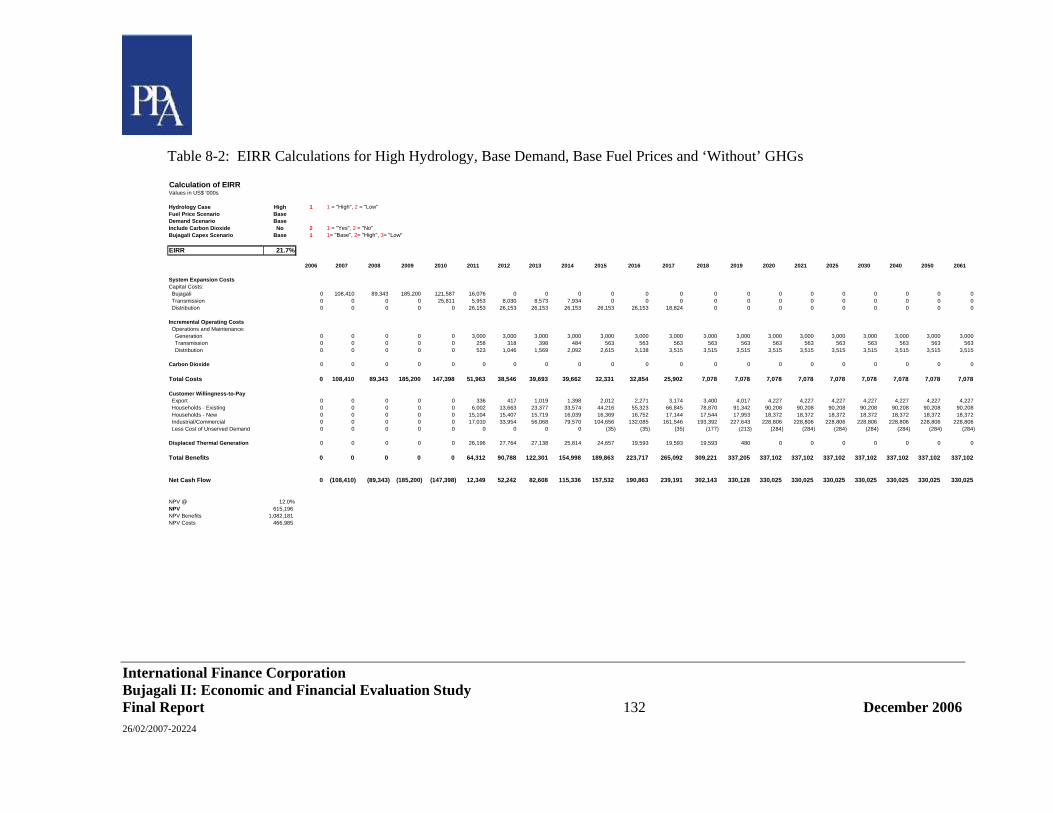
International Finance Corporation Bujagali II: Economic and Financial Evaluation Study Final Report 132 December 2006 26/02/2007-20224
Table 8-2: EIRR Calculations for High Hydrology, Base Demand, Base Fuel Prices and ‘Without’ GHGs
Calculation of EIRRValues in US$ '000s
Hydrology Case High 1 1 = "High", 2 = "Low"Fuel Price Scenario BaseDemand Scenario BaseInclude Carbon Dioxide No 2 1 = "Yes", 2 = "No"Bujagali Capex Scenario Base 1 1= "Base", 2= "High", 3= "Low"
EIRR 21.7%
2006 2007 2008 2009 2010 2011 2012 2013 2014 2015 2016 2017 2018 2019 2020 2021 2025 2030 2040 2050 2061
System Expansion CostsCapital Costs: Bujagali 0 108,410 89,343 185,200 121,587 16,076 0 0 0 0 0 0 0 0 0 0 0 0 0 0 0 Transmission 0 0 0 0 25,811 5,953 8,030 8,573 7,934 0 0 0 0 0 0 0 0 0 0 0 0 Distribution 0 0 0 0 0 26,153 26,153 26,153 26,153 26,153 26,153 18,824 0 0 0 0 0 0 0 0 0
Incremental Operating Costs Operations and Maintenance: Generation 0 0 0 0 0 3,000 3,000 3,000 3,000 3,000 3,000 3,000 3,000 3,000 3,000 3,000 3,000 3,000 3,000 3,000 3,000 Transmission 0 0 0 0 0 258 318 398 484 563 563 563 563 563 563 563 563 563 563 563 563 Distribution 0 0 0 0 0 523 1,046 1,569 2,092 2,615 3,138 3,515 3,515 3,515 3,515 3,515 3,515 3,515 3,515 3,515 3,515
Carbon Dioxide 0 0 0 0 0 0 0 0 0 0 0 0 0 0 0 0 0 0 0 0 0
Total Costs 0 108,410 89,343 185,200 147,398 51,963 38,546 39,693 39,662 32,331 32,854 25,902 7,078 7,078 7,078 7,078 7,078 7,078 7,078 7,078 7,078
Customer Willingness-to-Pay Export 0 0 0 0 0 336 417 1,019 1,398 2,012 2,271 3,174 3,400 4,017 4,227 4,227 4,227 4,227 4,227 4,227 4,227 Households - Existing 0 0 0 0 0 6,002 13,663 23,377 33,574 44,216 55,323 66,845 78,870 91,342 90,208 90,208 90,208 90,208 90,208 90,208 90,208 Households - New 0 0 0 0 0 15,104 15,407 15,719 16,039 16,369 16,752 17,144 17,544 17,953 18,372 18,372 18,372 18,372 18,372 18,372 18,372 Industrial/Commercial 0 0 0 0 0 17,010 33,954 56,068 79,570 104,656 132,085 161,546 193,392 227,643 228,806 228,806 228,806 228,806 228,806 228,806 228,806 Less Cost of Unserved Demand 0 0 0 0 0 0 0 0 0 (35) (35) (35) (177) (213) (284) (284) (284) (284) (284) (284) (284)
Displaced Thermal Generation 0 0 0 0 0 26,196 27,764 27,138 25,814 24,657 19,593 19,593 19,593 480 0 0 0 0 0 0 0
Total Benefits 0 0 0 0 0 64,312 90,788 122,301 154,998 189,863 223,717 265,092 309,221 337,205 337,102 337,102 337,102 337,102 337,102 337,102 337,102
Net Cash Flow 0 (108,410) (89,343) (185,200) (147,398) 12,349 52,242 82,608 115,336 157,532 190,863 239,191 302,143 330,128 330,025 330,025 330,025 330,025 330,025 330,025 330,025
NPV @ 12.0%NPV 615,196 NPV Benefits 1,082,181 NPV Costs 466,985

International Finance Corporation Bujagali II: Economic and Financial Evaluation Study Final Report 133 December 2006 26/02/2007-20224
Table 8-3: EIRR Calculations for Low Hydrology, Base Demand, Base Fuel Prices and ‘With’ GHGs
Calculation of EIRRValues in US$ '000s
Hydrology Case Low 2 1 = "High", 2 = "Low"Fuel Price Scenario BaseDemand Scenario BaseInclude Carbon Dioxide Yes 1 1 = "Yes", 2 = "No"Bujagali Capex Scenario Base 1 1= "Base", 2= "High", 3= "Low"
EIRR 22.9%
2006 2007 2008 2009 2010 2011 2012 2013 2014 2015 2016 2017 2018 2019 2020 2021 2025 2030 2040 2050 2061
System Expansion CostsCapital Costs: Bujagali 0 108,410 89,343 185,200 121,587 16,076 0 0 0 0 0 0 0 0 0 0 0 0 0 0 0 Transmission 0 0 0 0 25,811 5,953 8,030 8,573 7,934 0 0 0 0 0 0 0 0 0 0 0 0 Distribution 0 0 0 0 0 26,153 26,153 26,153 26,153 26,153 26,153 18,824 0 0 0 0 0 0 0 0 0
Incremental Operating Costs Operations and Maintenance: Generation 0 0 0 0 0 3,000 3,000 3,000 3,000 3,000 3,000 3,000 3,000 3,000 3,000 3,000 3,000 3,000 3,000 3,000 3,000 Transmission 0 0 0 0 0 258 318 398 484 563 563 563 563 563 563 563 563 563 563 563 563 Distribution 0 0 0 0 0 523 1,046 1,569 2,092 2,615 3,138 3,515 3,515 3,515 3,515 3,515 3,515 3,515 3,515 3,515 3,515
Carbon Dioxide 0 0 0 0 0 (20,378) (20) 0 0 0 0 (10,594) (15,067) (18,221) (20,091) (20,091) (20,091) (20,091) (20,091) (20,091) (20,091)
Total Costs 0 108,410 89,343 185,200 147,398 31,584 38,526 39,693 39,662 32,331 32,854 15,307 (7,989) (11,143) (13,014) (13,014) (13,014) (13,014) (13,014) (13,014) (13,014)
Customer Willingness-to-Pay Export 0 0 0 0 0 336 417 1,019 1,398 2,012 2,248 2,248 2,248 2,248 2,248 2,248 2,248 2,248 2,248 2,248 2,248 Households - Existing 0 0 0 0 0 6,002 13,663 23,377 33,574 44,216 54,769 61,636 61,636 61,636 61,636 61,636 61,636 61,636 61,636 61,636 61,636 Households - New 0 0 0 0 0 15,104 15,407 15,719 16,039 16,369 16,752 0 0 0 0 0 0 0 0 0 0 Industrial/Commercial 0 0 0 0 0 17,010 33,954 56,068 79,570 104,656 130,762 130,665 130,561 130,450 130,334 130,334 130,334 130,334 130,334 130,334 130,334 Less Cost of Unserved Demand 0 0 0 0 0 0 0 0 0 0 0 0 0 0 (36) (36) (36) (36) (36) (36) (36)
Displaced Thermal Generation 0 0 0 0 0 121,740 126,828 101,387 53,302 25,127 0 0 0 0 0 0 0 0 0 0 0
Total Benefits 0 0 0 0 0 159,856 189,852 196,549 182,486 190,369 202,283 192,301 192,197 192,086 191,935 191,935 191,935 191,935 191,935 191,935 191,935
Net Cash Flow 0 (108,410) (89,343) (185,200) (147,398) 128,271 151,326 156,857 142,824 158,038 169,429 176,994 200,186 203,229 204,948 204,948 204,948 204,948 204,948 204,948 204,948
NPV @ 12.0%NPV 475,902 NPV Benefits 888,688 NPV Costs 412,786
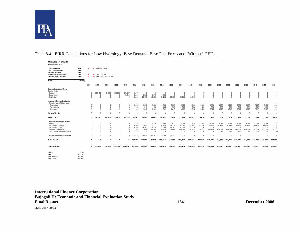
International Finance Corporation Bujagali II: Economic and Financial Evaluation Study Final Report 134 December 2006 26/02/2007-20224
Table 8-4: EIRR Calculations for Low Hydrology, Base Demand, Base Fuel Prices and ‘Without’ GHGs
Calculation of EIRRValues in US$ '000s
Hydrology Case Low 2 1 = "High", 2 = "Low"Fuel Price Scenario BaseDemand Scenario BaseInclude Carbon Dioxide No 2 1 = "Yes", 2 = "No"Bujagali Capex Scenario Base 1 1= "Base", 2= "High", 3= "Low"
EIRR 22.0%
2006 2007 2008 2009 2010 2011 2012 2013 2014 2015 2016 2017 2018 2019 2020 2021 2025 2030 2040 2050 2061
System Expansion CostsCapital Costs: Bujagali 0 108,410 89,343 185,200 121,587 16,076 0 0 0 0 0 0 0 0 0 0 0 0 0 0 0 Transmission 0 0 0 0 25,811 5,953 8,030 8,573 7,934 0 0 0 0 0 0 0 0 0 0 0 0 Distribution 0 0 0 0 0 26,153 26,153 26,153 26,153 26,153 26,153 18,824 0 0 0 0 0 0 0 0 0
Incremental Operating Costs Operations and Maintenance: Generation 0 0 0 0 0 3,000 3,000 3,000 3,000 3,000 3,000 3,000 3,000 3,000 3,000 3,000 3,000 3,000 3,000 3,000 3,000 Transmission 0 0 0 0 0 258 318 398 484 563 563 563 563 563 563 563 563 563 563 563 563 Distribution 0 0 0 0 0 523 1,046 1,569 2,092 2,615 3,138 3,515 3,515 3,515 3,515 3,515 3,515 3,515 3,515 3,515 3,515
Carbon Dioxide 0 0 0 0 0 0 0 0 0 0 0 0 0 0 0 0 0 0 0 0 0
Total Costs 0 108,410 89,343 185,200 147,398 51,963 38,546 39,693 39,662 32,331 32,854 25,902 7,078 7,078 7,078 7,078 7,078 7,078 7,078 7,078 7,078
Customer Willingness-to-Pay Export 0 0 0 0 0 336 417 1,019 1,398 2,012 2,248 2,248 2,248 2,248 2,248 2,248 2,248 2,248 2,248 2,248 2,248 Households - Existing 0 0 0 0 0 6,002 13,663 23,377 33,574 44,216 54,769 61,636 61,636 61,636 61,636 61,636 61,636 61,636 61,636 61,636 61,636 Households - New 0 0 0 0 0 15,104 15,407 15,719 16,039 16,369 16,752 0 0 0 0 0 0 0 0 0 0 Industrial/Commercial 0 0 0 0 0 17,010 33,954 56,068 79,570 104,656 130,762 130,665 130,561 130,450 130,334 130,334 130,334 130,334 130,334 130,334 130,334 Less Cost of Unserved Demand 0 0 0 0 0 0 0 0 0 0 0 0 0 0 (36) (36) (36) (36) (36) (36) (36)
Displaced Thermal Generation 0 0 0 0 0 121,740 126,828 101,387 53,302 25,127 0 0 0 0 0 0 0 0 0 0 0
Total Benefits 0 0 0 0 0 159,856 189,852 196,549 182,486 190,369 202,283 192,301 192,197 192,086 191,935 191,935 191,935 191,935 191,935 191,935 191,935
Net Cash Flow 0 (108,410) (89,343) (185,200) (147,398) 107,893 151,306 156,857 142,824 158,038 169,429 166,400 185,119 185,008 184,857 184,857 184,857 184,857 184,857 184,857 184,857
NPV @ 12.0%NPV 421,703 NPV Benefits 888,688 NPV Costs 466,985
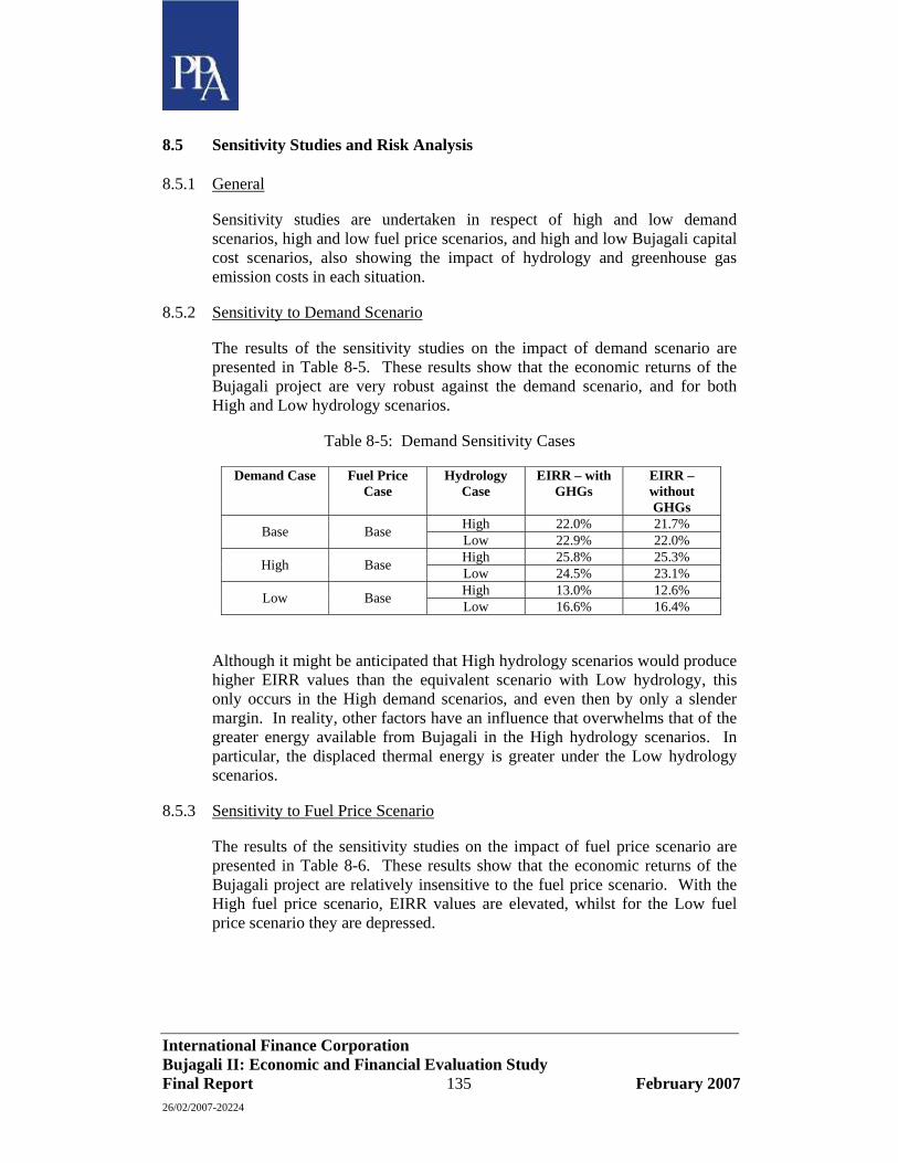
International Finance Corporation Bujagali II: Economic and Financial Evaluation Study Final Report 135 February 2007 26/02/2007-20224
8.5 Sensitivity Studies and Risk Analysis
8.5.1 General
Sensitivity studies are undertaken in respect of high and low demand scenarios, high and low fuel price scenarios, and high and low Bujagali capital cost scenarios, also showing the impact of hydrology and greenhouse gas emission costs in each situation.
8.5.2 Sensitivity to Demand Scenario
The results of the sensitivity studies on the impact of demand scenario are presented in Table 8-5. These results show that the economic returns of the Bujagali project are very robust against the demand scenario, and for both High and Low hydrology scenarios.
Table 8-5: Demand Sensitivity Cases
Demand Case Fuel Price Case
Hydrology Case
EIRR – with GHGs
EIRR – without GHGs
High 22.0% 21.7% Base Base Low 22.9% 22.0% High 25.8% 25.3% High Base Low 24.5% 23.1% High 13.0% 12.6% Low Base Low 16.6% 16.4%
Although it might be anticipated that High hydrology scenarios would produce higher EIRR values than the equivalent scenario with Low hydrology, this only occurs in the High demand scenarios, and even then by only a slender margin. In reality, other factors have an influence that overwhelms that of the greater energy available from Bujagali in the High hydrology scenarios. In particular, the displaced thermal energy is greater under the Low hydrology scenarios.
8.5.3 Sensitivity to Fuel Price Scenario
The results of the sensitivity studies on the impact of fuel price scenario are presented in Table 8-6. These results show that the economic returns of the Bujagali project are relatively insensitive to the fuel price scenario. With the High fuel price scenario, EIRR values are elevated, whilst for the Low fuel price scenario they are depressed.
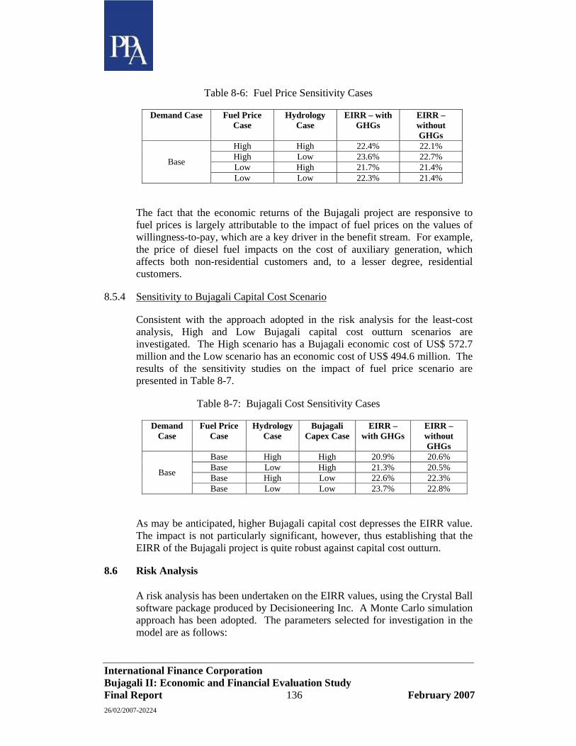
International Finance Corporation Bujagali II: Economic and Financial Evaluation Study Final Report 136 February 2007 26/02/2007-20224
Table 8-6: Fuel Price Sensitivity Cases
Demand Case Fuel Price Case
Hydrology Case
EIRR – with GHGs
EIRR – without GHGs
High High 22.4% 22.1% High Low 23.6% 22.7% Low High 21.7% 21.4% Base
Low Low 22.3% 21.4%
The fact that the economic returns of the Bujagali project are responsive to fuel prices is largely attributable to the impact of fuel prices on the values of willingness-to-pay, which are a key driver in the benefit stream. For example, the price of diesel fuel impacts on the cost of auxiliary generation, which affects both non-residential customers and, to a lesser degree, residential customers.
8.5.4 Sensitivity to Bujagali Capital Cost Scenario
Consistent with the approach adopted in the risk analysis for the least-cost analysis, High and Low Bujagali capital cost outturn scenarios are investigated. The High scenario has a Bujagali economic cost of US$ 572.7 million and the Low scenario has an economic cost of US$ 494.6 million. The results of the sensitivity studies on the impact of fuel price scenario are presented in Table 8-7.
Table 8-7: Bujagali Cost Sensitivity Cases
Demand Case
Fuel Price Case
Hydrology Case
Bujagali Capex Case
EIRR – with GHGs
EIRR – without GHGs
Base High High 20.9% 20.6% Base Low High 21.3% 20.5% Base High Low 22.6% 22.3% Base
Base Low Low 23.7% 22.8%
As may be anticipated, higher Bujagali capital cost depresses the EIRR value. The impact is not particularly significant, however, thus establishing that the EIRR of the Bujagali project is quite robust against capital cost outturn.
8.6 Risk Analysis
A risk analysis has been undertaken on the EIRR values, using the Crystal Ball software package produced by Decisioneering Inc. A Monte Carlo simulation approach has been adopted. The parameters selected for investigation in the model are as follows:

International Finance Corporation Bujagali II: Economic and Financial Evaluation Study Final Report 137 February 2007 26/02/2007-20224
o Demand forecast;
o Crude oil price;
o Bujagali capital cost;
o T&D capital costs;
o Willingness-to-pay of newly-connected residential customers; and
o Hydrology.
The ranges and probability assumptions for each parameter are presented in the following paragraphs.
Demand Forecast: A discrete uniform distribution is adopted, with a 30% probability of Low demand, 40% probability of Base demand, and 30% probability of High demand.
Crude Oil Price: The crude oil price range adopted in the least-cost analysis assumed that, for all years, the Low price is 66.2% of the Base price, and the High price is 147.9% of the Base price. A log normal distribution has been adopted with a standard deviation equal to 35% of the mean, such that the probabilities of the crude oil price falling below 66.2% of the mean, and above 147.9% of the mean are each approximately 10%.
Bujagali Capex: A discrete uniform distribution is adopted, with a 20% probability of Low Bujagali capex (US$ 494.6 million), 60% probability of Base Bujagali capex (US$ 520.6 million), and 20% probability of High Bujagali capex (US$ 572.7 million).
T&D Capex: A normal distribution of costs is assumed, with the mean of the distribution coincident with the Base cost estimate. The standard deviation of the distribution is assumed to be 5% of the Base cost.
WTP for Newly-Connected Residential Customers: The WTP value is assumed to have two components. The first component, relating to the tariff, is assumed to be not subject to uncertainty. The second component, however, relates to the consumer surplus, for which a triangular probability distribution is adopted. Zero consumer surplus is assumed to have zero probability, whilst the Base value of consumer surplus is assumed to have maximum probability of occurrence. Zero probability of the consumer surplus exceeding the Base value is also adopted.
Hydrology: A Yes/No function is proposed, with a 79%/21% split of probability of the Low/High hydrology.
Greenhouse Gases Credit: The two options for greenhouse gases – inclusion or exclusion – are not incorporated into the risk model, and the two scenarios are examined separately.
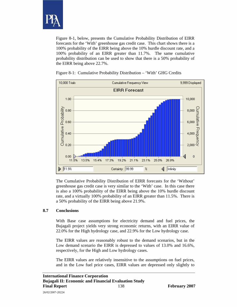
International Finance Corporation Bujagali II: Economic and Financial Evaluation Study Final Report 138 February 2007 26/02/2007-20224
Figure 8-1, below, presents the Cumulative Probability Distribution of EIRR forecasts for the ‘With’ greenhouse gas credit case. This chart shows there is a 100% probability of the EIRR being above the 10% hurdle discount rate, and a 100% probability of an EIRR greater than 11.7%. The same cumulative probability distribution can be used to show that there is a 50% probability of the EIRR being above 22.7%.
Figure 8-1: Cumulative Probability Distribution – ‘With’ GHG Credits
The Cumulative Probability Distribution of EIRR forecasts for the ‘Without’ greenhouse gas credit case is very similar to the ‘With’ case. In this case there is also a 100% probability of the EIRR being above the 10% hurdle discount rate, and a virtually 100% probability of an EIRR greater than 11.5%. There is a 50% probability of the EIRR being above 21.9%.
8.7 Conclusions
With Base case assumptions for electricity demand and fuel prices, the Bujagali project yields very strong economic returns, with an EIRR value of 22.0% for the High hydrology case, and 22.9% for the Low hydrology case.
The EIRR values are reasonably robust to the demand scenarios, but in the Low demand scenario the EIRR is depressed to values of 13.0% and 16.6%, respectively, for the High and Low hydrology cases.
The EIRR values are relatively insensitive to the assumptions on fuel prices, and in the Low fuel price cases, EIRR values are depressed only slightly to

International Finance Corporation Bujagali II: Economic and Financial Evaluation Study Final Report 139 February 2007 26/02/2007-20224
values of 21.7% and 22.3%, respectively, for the High and Low hydrology cases.
The EIRR values are also relatively insensitive to the outturn in the Bujagali capital cost. The High scenario Bujagali capital cost outturn depresses the EIRR only very slightly, to 20.9% in the High hydrology case, and 21.3% in the Low hydrology case.
Risk analysis using a proprietary software package has been undertaken, to further test the robustness of the EIRR to outcomes on several key parameters. This analysis also shows that there is a 100% probability of the Bujagali EIRR being greater than the 10% hurdle discount rate. When greenhouse gas credits are included, there is 100% probability of an EIRR greater than 11.7%, and this reduces only very slightly, to 11.5%, when greenhouse gas credits are not included. The cumulative probability distributions from these analyses shows that there is a 50% probability of the EIRR being greater than 22.7% when greenhouse gas credits are included, and 21.9% when greenhouse gas credits are not included.
In conclusion, the expected economic return of the Bujagali project is high and very robust to adverse outturns in the key parameters.
International Finance Corporation Bujagali II: Economic and Financial Evaluation Study Final Report 140 February 2007 26/02/2007-20224
9 Financial Feasibility
9.1 Objectives and outputs
The objective of this task has been to examine the likely evolution of end-user tariffs, and to compare these with the assumptions of the demand forecast. Should there be discrepancies between the tariff outcome and the tariff entering the initial assumptions, the intention is to revise the tariff assumptions underlying the demand forecast and re-iterate demand and supply at the new prices.
The ToR requires that the determination of tariffs should be consistent with regulatory practice in Uganda, i.e. based on cost-reflective principles with phase-out of subsidies or cross-subsidies based on the policies of the regulator. Further, allowance may be made for tariff stabilisation, i.e. the use of a surcharge on tariffs in order to smooth out price instabilities arising from new generation.
The ToR required that the analysis be taken forward to 2012, with constant tariffs in real terms thereafter. Detailed tariff calculations have been undertaken to 2012 (including tariff structures). Thereafter, we have examined evolution in average costs, in order to take into account new investments post Bujagali – essentially to test whether these new investments will result in a tariff shock that undermines the assumption of constant real tariffs.
The work has been structured in four sub-tasks:
• Review of tariff methodology;
• Review of tariff models and model development;
• Data collection; and
• Preparation of results.
Each of these tasks is reported on below.
9.2 Review of tariff methodology
The Electricity Regulatory Authority (ERA) of Uganda implements a tariff methodology for existing licences in generation (Eskom Uganda) and distribution (Umeme) that is contained in the licences of the respective entities. For transmission (UETCL), the tariff methodology is not formalised in the licences, and is more subject to regulatory discretion.

International Finance Corporation Bujagali II: Economic and Financial Evaluation Study Final Report 141 February 2007 26/02/2007-20224
9.2.1 Tariff methodology for existing licensed generators
The tariff methodology for Eskom Uganda is fairly straightforward and allows pass-through of costs. Incentive elements in the tariff are firstly in operating costs, where allowable costs are set in the licence for a seven year period; and secondly in availability measures.
The cost components of Eskom Uganda’s revenue requirement are:
• Lease payments for UEGCL assets: these are based on the cash flow requirements of UEGCL and can be projected based on changes in the debt and interest payments of UEGCL.
• Operating and maintenance (O&M) costs: these are as set in the licence as allowed expenditures rather than actual expenditure. Regulatory fees are in addition to the O&M allowances.
• Depreciation and return: on accumulated investment (gross and net respectively) by Eskom Uganda, as well as return on working capital, at the set rate of return in the licence.
• Taxation on return.
Certain elements of the revenue requirement are indexed to exchange rates and inflation rates. Lease payments are set in dollars, and so indexed to exchange rates. O&M costs are partly expressed in shillings and partly in dollars, with the former indexed to Ugandan inflation and the latter to US inflation and the exchange rate.
For the purposes of modelling end-user tariffs, it is adequate to model the revenue requirement of Eskom Uganda and not translate this into the capacity price (USh per MW made available) as billed to UETCL. That is, the revenue requirement can be treated as equivalent to a capacity payment in a power purchase agreement.
9.2.2 Tariff methodology for other licensed generators
Other licensed generators selling power to UETCL are the two mini-hydros (KCCL and Kilembe). These generators are on power purchase agreements at unit rates per kWh sold. These prices are indexed to the Bulk Supply Tariff (BST).
In addition there is the existing 50MW Aggreko thermal generator (Aggreko I) on a PPA with the following components:
• Capacity payments: US$ 45.9 per MW per hour available – equivalent to an annual cost of US$ 9.9 million.
International Finance Corporation Bujagali II: Economic and Financial Evaluation Study Final Report 142 February 2007 26/02/2007-20224
• O&M: 0.95 US¢/kWh supplied
• Fuel logistics: 5.83 US¢/kWh supplied
• Fuel purchase: FOB price. During 2005 this has averaged US$ 0.42/litre and a consumption of 0.27 l/kWh (maximum guaranteed by Aggreko is 0.28).
• Fuel duty: During 2005 this has averaged US$ 0.26/litre, which is 62% of the FOB price.
9.2.3 Tariff methodology for planned and future generators
Future generators will be assumed to hold a PPA with UETCL at a price that reflects their costs. The actual generators to include are derived from the generation expansion plan, and include:
• Additional small scale hydro: at fixed feed-in tariff rates as set by ERA;
• Thermal (committed and future): pass-through of fuel and operating costs, plus a capacity payment;
• Geothermal: pass-through of operating costs and a capacity payment;
• Additional large scale hydro: entire price as a capacity payment to reflect full financial costs in dollar terms.
All thermal generators are assumed to be exempt from fuel taxes.
9.2.4 Tariff methodology for UETCL
The tariff methodology for UETCL comprises two parts:
• Firstly, a pass-through of all generation costs (described above), with an adjustment for losses; and
• Secondly, a pass-through of UETCL’s costs.
The second component would normally be based on a typical revenue requirement, including depreciation and return elements. At present, ERA has not formalised the tariff methodology for UETCL and has in the recent past been awarding a revenue requirement that meets its cash flow requirements (without any allowance for return on equity). ERA is in the process of preparing a tariff methodology for UETCL. While this process has not reached its conclusion yet, a discussion paper has been provided to us. The
International Finance Corporation Bujagali II: Economic and Financial Evaluation Study Final Report 143 February 2007 26/02/2007-20224
discussion paper indicates that ERA plans to establish a revenue requirement that includes:
• O&M costs;
• Depreciation;
• Interest payments for debt in hand at the start of the process (e.g. end 2006);
• Return on investment made after the start of the process (e.g. from 2006);
• Less other sources of revenue, including export revenues.
In addition, UETCL has in the past included a component to accrue a tariff stabilisation fund and a component to accrue a liquidity fund. ERA expects that neither of these components will be required in the future. This is discussed later in this report.
Finally, UETCL pays a rural electrification levy of 5% on electricity purchased from generators for resale within Uganda.
The tariff structure that UETCL charges to Umeme is a time-of-use tariff in three time bands: peak, shoulder and off-peak. The shoulder tariff is set to UETCL’s average tariff (i.e. unit revenue requirement).The peak tariff is set at 35% higher than the shoulder tariff, and the off-peak is set to balance the revenue requirement.
9.2.5 Tariff methodology for Umeme
The tariff methodology for Umeme has two components: the power supply tariff and the distribution margin.
The power supply tariff is simply the Bulk Supply Tariff charged by UETCL adjusted for losses and load profile per customer group. Losses are differentiated by voltage level (LV and MV) so that different customer groups will have different power supply tariffs. In ERA’s application of the methodology, commercial losses are set equal for all tariff categories. Load profiles differ by customer group and so this will also influence power supply tariffs.
The tariff methodology allows for reconciliation between Umeme’s actual costs of power purchase and end-user revenues. This means that any reductions in the cost of losses arising from loss improvements are transferred to customers and not retained by Umeme. The incentive for Umeme to reduce losses lies in the determination of network prices, which are based on
International Finance Corporation Bujagali II: Economic and Financial Evaluation Study Final Report 144 February 2007 26/02/2007-20224
regulatory loss factors. The consequence of this for the financial modelling is that the loss factors to use for the power supply tariff should be the actual losses and not the regulatory allowances.
The distribution margin is built up in a similar way to Eskom Uganda’s costs. There is allowance for:
• Lease payments for UEDCL assets: these are based on the cash flow requirements of UEDCL and can be projected based on changes in the debt and interest payments of UEDCL.
• Operating and maintenance (O&M) costs: these are as set in the licence as allowed expenditures rather than actual expenditure, adjusted by the efficiency factor as set in the licence. As with Eskom generation, the O&M costs are partly indexed to Ugandan inflation and partly to US inflation and exchange rate. Regulatory fees and once-off stamp tax are in addition to the O&M allowances.
• Depreciation and return: on accumulated investment (gross and net respectively) by Umeme, as well as return on working capital, with the (after-tax) rate of return set in the licence. It should be noted that where debt is on concessionary terms, the assets funded do not attract a return, and instead actual interest charges are passed through.
• Taxation on the allowed return at 30%.
The tariff methodology for Umeme has some special features dealing with uncollected debt. In the first year (2005), a lump sum allowance was given. Thereafter, a percentage uplift on the overall revenue requirement (including pass through of generation costs) was permitted. A transition credit was also provided in the first year, to reduce the overall revenue requirement by US$ 5 million. Lastly, any other revenues are deducted from the revenue requirement.
The tariff methodology has an approach to allocating the revenue requirement to customer groups and so arriving at a distribution margin per customer category. This approach has the following features:
• Firstly, costs are allocated to HV and LV levels. Customers on HV only pay for HV costs where customers on LV pay for both. The HV:LV split is 40:60.
• Secondly, costs at both the HV and LV levels are expressed as average unit costs (USh/kWh) based on the energy flowing into that voltage level. This cost is then used to derive peak, shoulder and off-peak costs where the shoulder cost is equal to the average cost, the peak cost is 20% higher and the off-peak cost is the residual cost. A weighted
International Finance Corporation Bujagali II: Economic and Financial Evaluation Study Final Report 145 February 2007 26/02/2007-20224
average tariff for each tariff category is then computed based on the load factors at each tariff level and the losses at each voltage level.
The energy volumes used for this calculation are based on the preceding year’s end-user sales. To determine the energy volumes at voltage levels other than at the end-use point, the sales volumes are adjusted by loss allowances rather than actual losses.
There is a “generation levy” of 0.3 per cent of the retail price to all customer categories. This forms part of the funding of the regulator.
9.2.6 Subsidies
There are several items where subsidies occur in the tariff methodology. These all occur during the period up to 2011, when Bujagali is commissioned. Thereafter, the tariff analysis assumes there would be no subsidies in the tariff. The subsidies in the pre-Bujagali period occur from:
• Firstly, not all the costs of the existing Aggreko thermal plant are passed through to end-users. The capacity payments are to Government’s account, and fuel duties are rebated (we also assume that fuel rebates are given for all thermal plant).
• Secondly, the HFO thermal plant is intended to be transferred to UETCL in 2012 free of charge. Thereafter, there will be no costs reflected in tariffs related to UETCL’s ownership of this plant.
• Thirdly, Government has in the past provided a subsidy to end-users in the form of a rebate on Umeme’s purchases from UETCL. ERA allocates the benefit of this rebate to different tariff categories. That is, ERA determines the cost reflective price per tariff category, and then deducts a subsidy for each tariff category so that the total subsidy equals the rebate.
It was initially anticipated that the subsidy to end-users referred to above would be phased-out by end-2007. However, it seems likely that subsidies will persist for some time given the high costs of thermal energy up to the commissioning of the next large hydropower project.
Tariffs are intended not to have any cross-subsidies between customer categories. The only cross-subsidy is for a life-line offered to domestic households for the first 15 kWh consumed per month. The cross-subsidy required to support this measure is only applied to other domestic consumers and is approximately 20 USh/kWh. However, the parameters that allocate costs across customer categories are set by the regulator, and are not explicitly linked to cost-structures. Hence, tariff structures may differ from the underlying cost-structures.

International Finance Corporation Bujagali II: Economic and Financial Evaluation Study Final Report 146 February 2007 26/02/2007-20224
9.2.7 Tariff stabilisation
ERA has required UETCL to include a tariff stabilisation charge in its revenue requirement and use this charge to build a stabilisation fund. This fund was originally intended to be used to buy down the costs of Bujagali power in the initial years so that any tariff adjustments could be phased in.
The amount included in UETCL’s revenue requirement has been 17.5 billion USh in both 2004 and 2005. For 2006 tariffs, there is no tariff stabilisation charge. ERA hopes that the tariff stabilisation charge can be reinstated in 2008, although it is not evident that this will occur.
Given that from 2007 through to 2010, the costs of generation are likely to be high (and higher than after the commissioning of Bujagali), we assume that there will be no tariff stabilisation charge in the period to 2010. That is, during the period when thermal capacity is extensively used, the stabilisation charge will be removed as a measure to contain the impact on end-user tariffs.
9.3 Review of tariff models and model development
There are four different tariff models that are currently available for the Ugandan power sector:
• Firstly, there is the model developed by PA Consulting Group as part of the transaction advice to the Minister of Finance in relation to the privatisation of generation and distribution assets. This model builds up the basic revenue requirement of each element of the industry over a forecast period. However, it does not determine end-user tariffs, which are handled in a separate model that is not structured for forecasting. Further, the model does not accommodate generation costs other than Kiira/Nalubaale and Bujagali, does not include an energy balance to estimate emergency thermal energy production, nor is the tariff stabilisation fund incorporated.
• Secondly, there is the tariff model applied by ERA and developed by ECON. This model is developed for an annual tariff determination, but does have a seven year forecasting ability. It also fully captures all financial costs in the industry according to the licences that are currently in place. It does not deal with the costs of new generators except for allowing an input cost and volume.
• Thirdly, there is the tariff stabilisation fund model developed for ERA and MEMD by ECON. This model focuses on developments in the generation sector and forecasts the bulk sales tariff taking into account all sources of generation and tariff stabilisation measures. It also incorporates an energy balance to determine volumes from each generator.
International Finance Corporation Bujagali II: Economic and Financial Evaluation Study Final Report 147 February 2007 26/02/2007-20224
• Fourthly, there is a financial model of the sector developed for the World Bank by an independent consultant. This model builds up the cost structure of the industry in detail, including a variety of new thermal generation plan. It treats new large-scale hydro plant as a fixed price PPA in dollars. It derives average tariffs, but does not differentiate between end-use sector.
The model developed for the World Bank has a cost structure for UETCL that is based on cash flow requirements rather than a normal regulatory revenue requirement. The cost components (excluding generation costs) for UETCL are made up of:
• O&M costs;
• Interest payments;
• Loan repayments;
• Investment not funded by debt or grants;
• Less other sources of revenue, including export revenues.
Hence, the cost build up for UETCL must be amended to fit with ERA’s proposed tariff methodology for UETCL, which is closer to a standard revenue requirement calculation.
It was decided that the model developed for the World Bank would be used to derive certain of the revenue requirements and cost structure, and that the ERA model be used to derive tariffs. Costs for new generation plant are derived from the results of the least-cost expansion modelling.
The figure below presents the modelling tool that was developed in Microsoft Excel (except for the WASP program). The file labelled “Consolidated Data Inputs and Assumptions” brings together all the input from various sources and provides the source input for the ERA tariff model. This in turn provides detailed tariff structures up to 2012. The results from the tariff model are then assembled in the file labelled “Consolidated Results”, which then converts to constant 2006 prices, extends the analysis to 2020 (with average costs not detailed tariffs), compares the results with the tariff assumptions, and calculates subsidy requirements in cases where tariff assumptions are below the cost of supply.
The analysis has been undertaken for the “base” case, i.e. the least-cost expansion plan for the low hydrology, base demand forecast, and base thermal cost assumptions (designated Case 32).
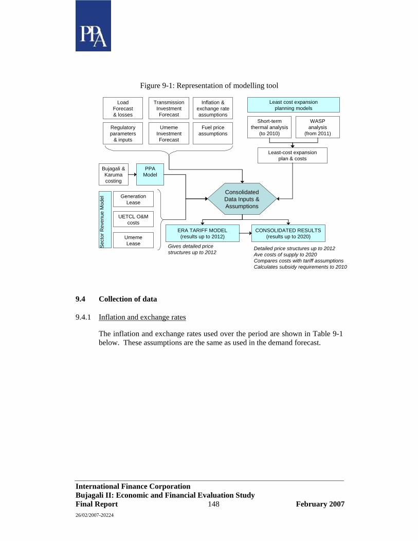
International Finance Corporation Bujagali II: Economic and Financial Evaluation Study Final Report 148 February 2007 26/02/2007-20224
Figure 9-1: Representation of modelling tool
9.4 Collection of data
9.4.1 Inflation and exchange rates
The inflation and exchange rates used over the period are shown in Table 9-1 below. These assumptions are the same as used in the demand forecast.
TransmissionInvestmentForecast
UmemeInvestmentForecast
Load Forecast & losses
Bujagali & Karuma costing
Least-cost expansion plan & costs
Short-termthermal analysis
(to 2010)
WASP analysis
(from 2011)
Inflation &exchange rateassumptions
Regulatory parameters
& inputs
Generation Lease
Umeme Lease
UETCL O&M costs
Sect
or R
even
ue M
odel
ConsolidatedData Inputs &Assumptions
Least cost expansion planning models
ERA TARIFF MODEL(results up to 2012)
CONSOLIDATED RESULTS (results up to 2020)
Gives detailed pricestructures up to 2012
Detailed price structures up to 2012 Ave costs of supply to 2020 Compares costs with tariff assumptionsCalculates subsidy requirements to 2010
PPA Model
Fuel priceassumptions

International Finance Corporation Bujagali II: Economic and Financial Evaluation Study Final Report 149 February 2007 26/02/2007-20224
Table 9-1: Inflation and exchange rate assumptions31
Inflation Exchange rate Year US Uganda Year end* Mid-year 2006 2.5 % 4.5 % 1,849 1,826 2007 2.5 % 4.5 % 1,894 1,871 2008 2.5 % 4.5 % 1,941 1,917 2009 2.5 % 4.5 % 1,988 1,964 2010 2.5 % 4.5 % 2,037 2,012
2011 2.5 % 4.5 % 2,087 2,061
2012** 2.5 % 4.5 % 2,138 2,112 * Initial exchange rate beginning 2006 is 1820.
** For assumptions post 2012, US and Ugandan inflation rates are assumed to be 2.5% and 4.5% p.a. respectively, and the exchange rate is assumed to depreciate at 2% per annum.
9.4.2 Demand forecast and losses
The demand forecast prepared for this study was used (see Section 2).
Umeme’s licence sets loss targets rather than passing through actual losses. The loss targets are only used for determining the distribution margin and not the power supply component of the tariff32. These loss targets for the first seven years (to end 2011) are shown Table 9-2 and compared with the distribution loss projections in the demand forecast. Following the introduction of thermal power and the resulting tariff increases, ERA will reset loss and collection rate allowances quarterly based on actual losses and collection rates, less an incentive.
31 These assumptions are broadly consistent with those assumptions made in the GDP forecasts by the IMF for GDP forecasting. The GDP forecasts assume an average Ugandan inflation over the period of 4.4% compared with the 4.5% assumed above. The exchange rate assumptions above are within 2% of those used in the GDP forecast.
32 In the regulatory tariff methodology, the regulatory loss targets are used to determine the pass through of the bulk supply tariff to end-users, i.e. the power supply price element of retail tariffs. However, the tariff methodology has a reconciliation of actual power supply costs against power supply revenues. This means that any reduction in the cost of losses is passed through to customers through the reconciliation mechanism. To date, ERA and Umeme have not applied the reconciliation, but in future it is expected to become more important as loss targets and actual losses diverge.

International Finance Corporation Bujagali II: Economic and Financial Evaluation Study Final Report 150 February 2007 26/02/2007-20224
Table 9-2: Loss assumptions and regulatory loss parameters
Year Regulatory distribution loss factor*
Load forecast distribution losses**
2006 33.9% 38.0% 2007 31.8% 35.1% 2008 30.6% 32.3% 2009 29.8% 29.4% 2010 29.0% 25.6% 2011 28.1% 22.0% 2012 21.3%*** 19.5%
* Adjusted to calendar year basis ** After subtracting transmission losses from total losses *** The regulatory loss factors for 2006-2011 are based on figures in Umeme’s
licence. The loss factor for 2012 is based on the assumption that the improvements in losses (in the demand forecast) will be used to set loss targets from 2012 onwards.
9.4.3 Generation costs
Generation costs are made up of the following:
• Eskom Uganda;
• Embedded generators (small scale hydro and bagasse – both existing and new);
• Existing and committed thermal power plants;
• New thermal and geothermal power plants;
• New large-scale hydropower.
Costs for Eskom Uganda are made up by its revenue requirement as described in the tariff methodology above. Costs are fixed and not variable, and so the same payment must be made regardless of power output. The cost calculations result in the annual costs to be paid to Eskom Uganda, shown in Table 9-3, expressed in constant 2006 US dollar terms.

International Finance Corporation Bujagali II: Economic and Financial Evaluation Study Final Report 151 February 2007 26/02/2007-20224
Table 9-3: Eskom capacity charges to UETCL, in constant 2006 US$ million
Year US$ million
2006 16.2
2007 15.9
2008 15.2
2009 15.0
2010 14.6
2011 14.3
2012 13.9
There are two existing small scale hydro plants (KCCL and Kilembe mines). KCCL is expected to be a self-generator from 2006 and will not supply to the grid. Kilembe Mines provides power at the prevailing bulk supply tariff.
The Kakira power plant should deliver 12 MW from 2007 for 18 hours per day. The average price for peak power is 5.25 US¢/kWh and for off-peak is 5.6 US¢/kWh.33.
The output of future small-scale renewable energy generators (small scale hydro and bagasse) was modelled in the short-term thermal analysis. Production was assumed to ramp up to an output of 350 GWh by 2009 and then was kept constant. A report to ERA in 2005 recommended a feed-in tariff scheme set out Table 9-4 below. We anticipate that the majority of small-scale hydro will be run-of-river, implying that the average tariff will apply rather than the peak tariff.
Table 9-4: Power prices for embedded renewable energy generators (constant 2006 US¢/kWh)
Years 1 – 5 Years 6 - 15 Peak 12.00 9.00 Shoulder 6.00 4.50 Off-peak 2.00 1.00 Average 6.67 4.56
33 The price structure is a result of two different set of price negotiations for the plant, where the initial 6 MW off-take was priced lower than the second 6 MW.
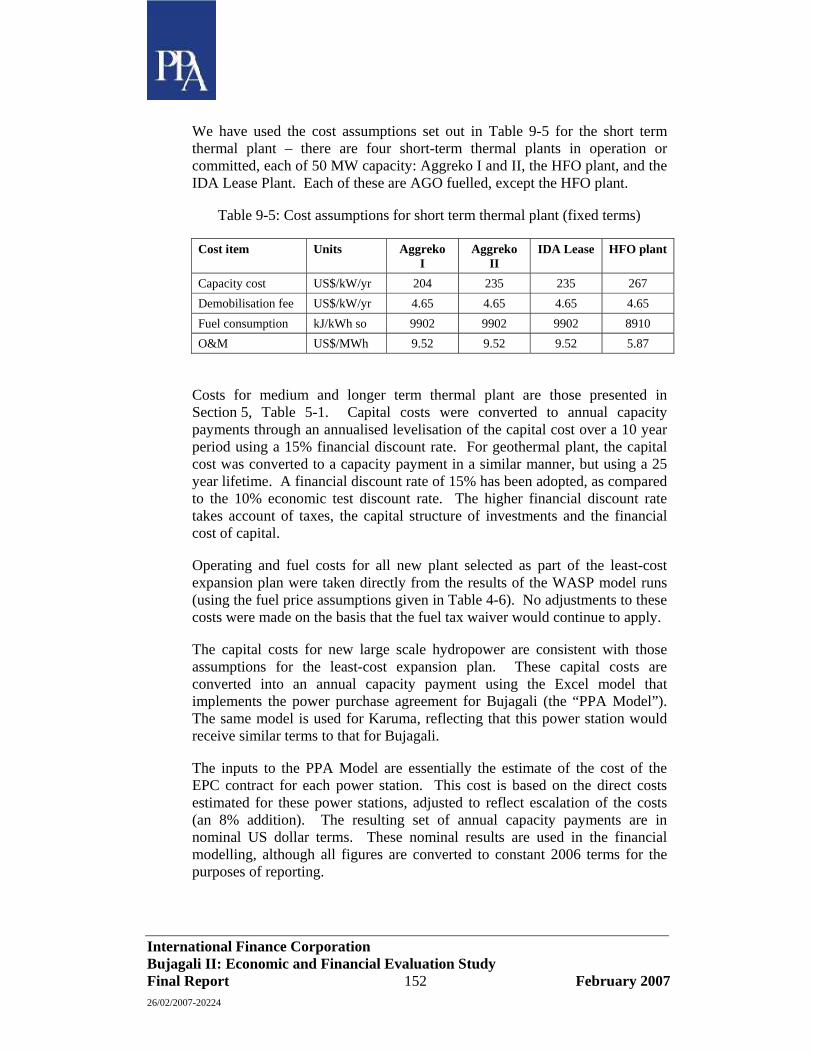
International Finance Corporation Bujagali II: Economic and Financial Evaluation Study Final Report 152 February 2007 26/02/2007-20224
We have used the cost assumptions set out in Table 9-5 for the short term thermal plant – there are four short-term thermal plants in operation or committed, each of 50 MW capacity: Aggreko I and II, the HFO plant, and the IDA Lease Plant. Each of these are AGO fuelled, except the HFO plant.
Table 9-5: Cost assumptions for short term thermal plant (fixed terms)
Cost item Units Aggreko I
Aggreko II
IDA Lease HFO plant
Capacity cost US$/kW/yr 204 235 235 267 Demobilisation fee US$/kW/yr 4.65 4.65 4.65 4.65 Fuel consumption kJ/kWh so 9902 9902 9902 8910 O&M US$/MWh 9.52 9.52 9.52 5.87
Costs for medium and longer term thermal plant are those presented in Section 5, Table 5-1. Capital costs were converted to annual capacity payments through an annualised levelisation of the capital cost over a 10 year period using a 15% financial discount rate. For geothermal plant, the capital cost was converted to a capacity payment in a similar manner, but using a 25 year lifetime. A financial discount rate of 15% has been adopted, as compared to the 10% economic test discount rate. The higher financial discount rate takes account of taxes, the capital structure of investments and the financial cost of capital.
Operating and fuel costs for all new plant selected as part of the least-cost expansion plan were taken directly from the results of the WASP model runs (using the fuel price assumptions given in Table 4-6). No adjustments to these costs were made on the basis that the fuel tax waiver would continue to apply.
The capital costs for new large scale hydropower are consistent with those assumptions for the least-cost expansion plan. These capital costs are converted into an annual capacity payment using the Excel model that implements the power purchase agreement for Bujagali (the “PPA Model”). The same model is used for Karuma, reflecting that this power station would receive similar terms to that for Bujagali.
The inputs to the PPA Model are essentially the estimate of the cost of the EPC contract for each power station. This cost is based on the direct costs estimated for these power stations, adjusted to reflect escalation of the costs (an 8% addition). The resulting set of annual capacity payments are in nominal US dollar terms. These nominal results are used in the financial modelling, although all figures are converted to constant 2006 terms for the purposes of reporting.
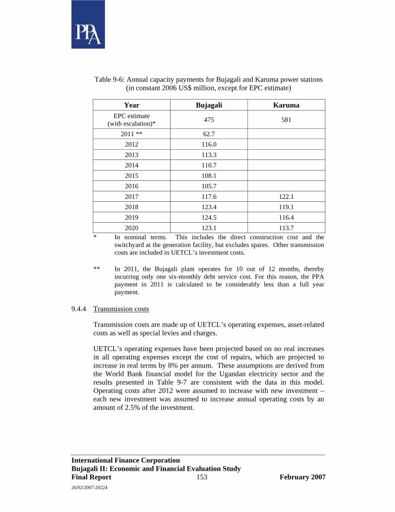
International Finance Corporation Bujagali II: Economic and Financial Evaluation Study Final Report 153 February 2007 26/02/2007-20224
Table 9-6: Annual capacity payments for Bujagali and Karuma power stations (in constant 2006 US$ million, except for EPC estimate)
Year Bujagali Karuma EPC estimate
(with escalation)* 475 581
2011 ** 62.7 2012 116.0 2013 113.3 2014 110.7 2015 108.1 2016 105.7 2017 117.6 122.1 2018 123.4 119.1 2019 124.5 116.4 2020 123.1 113.7
* In nominal terms. This includes the direct construction cost and the switchyard at the generation facility, but excludes spares. Other transmission costs are included in UETCL’s investment costs.
** In 2011, the Bujagali plant operates for 10 out of 12 months, thereby incurring only one six-monthly debt service cost. For this reason, the PPA payment in 2011 is calculated to be considerably less than a full year payment.
9.4.4 Transmission costs
Transmission costs are made up of UETCL’s operating expenses, asset-related costs as well as special levies and charges.
UETCL’s operating expenses have been projected based on no real increases in all operating expenses except the cost of repairs, which are projected to increase in real terms by 8% per annum. These assumptions are derived from the World Bank financial model for the Ugandan electricity sector and the results presented in Table 9-7 are consistent with the data in this model. Operating costs after 2012 were assumed to increase with new investment – each new investment was assumed to increase annual operating costs by an amount of 2.5% of the investment.
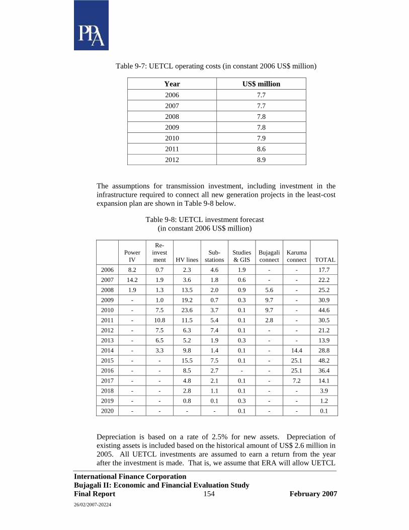
International Finance Corporation Bujagali II: Economic and Financial Evaluation Study Final Report 154 February 2007 26/02/2007-20224
Table 9-7: UETCL operating costs (in constant 2006 US$ million)
Year US$ million 2006 7.7 2007 7.7 2008 7.8 2009 7.8 2010 7.9 2011 8.6 2012 8.9
The assumptions for transmission investment, including investment in the infrastructure required to connect all new generation projects in the least-cost expansion plan are shown in Table 9-8 below.
Table 9-8: UETCL investment forecast (in constant 2006 US$ million)
Power
IV
Re- invest ment HV lines
Sub- stations
Studies & GIS
Bujagali connect
Karuma connect TOTAL
2006 8.2 0.7 2.3 4.6 1.9 - - 17.7 2007 14.2 1.9 3.6 1.8 0.6 - - 22.2 2008 1.9 1.3 13.5 2.0 0.9 5.6 - 25.2 2009 - 1.0 19.2 0.7 0.3 9.7 - 30.9 2010 - 7.5 23.6 3.7 0.1 9.7 - 44.6 2011 - 10.8 11.5 5.4 0.1 2.8 - 30.5 2012 - 7.5 6.3 7.4 0.1 - - 21.2 2013 - 6.5 5.2 1.9 0.3 - - 13.9 2014 - 3.3 9.8 1.4 0.1 - 14.4 28.8 2015 - - 15.5 7.5 0.1 - 25.1 48.2 2016 - - 8.5 2.7 - - 25.1 36.4 2017 - - 4.8 2.1 0.1 - 7.2 14.1 2018 - - 2.8 1.1 0.1 - - 3.9 2019 - - 0.8 0.1 0.3 - - 1.2 2020 - - - - 0.1 - - 0.1
Depreciation is based on a rate of 2.5% for new assets. Depreciation of existing assets is included based on the historical amount of US$ 2.6 million in 2005. All UETCL investments are assumed to earn a return from the year after the investment is made. That is, we assume that ERA will allow UETCL
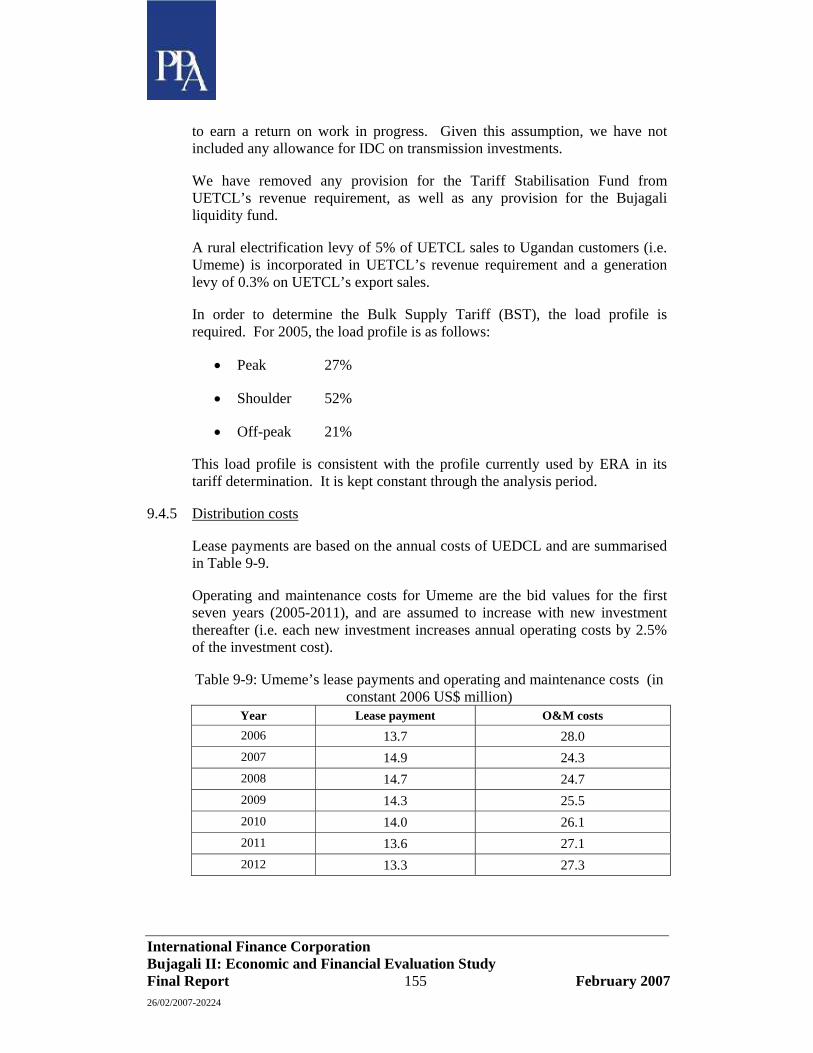
International Finance Corporation Bujagali II: Economic and Financial Evaluation Study Final Report 155 February 2007 26/02/2007-20224
to earn a return on work in progress. Given this assumption, we have not included any allowance for IDC on transmission investments.
We have removed any provision for the Tariff Stabilisation Fund from UETCL’s revenue requirement, as well as any provision for the Bujagali liquidity fund.
A rural electrification levy of 5% of UETCL sales to Ugandan customers (i.e. Umeme) is incorporated in UETCL’s revenue requirement and a generation levy of 0.3% on UETCL’s export sales.
In order to determine the Bulk Supply Tariff (BST), the load profile is required. For 2005, the load profile is as follows:
• Peak 27%
• Shoulder 52%
• Off-peak 21%
This load profile is consistent with the profile currently used by ERA in its tariff determination. It is kept constant through the analysis period.
9.4.5 Distribution costs
Lease payments are based on the annual costs of UEDCL and are summarised in Table 9-9.
Operating and maintenance costs for Umeme are the bid values for the first seven years (2005-2011), and are assumed to increase with new investment thereafter (i.e. each new investment increases annual operating costs by 2.5% of the investment cost).
Table 9-9: Umeme’s lease payments and operating and maintenance costs (in constant 2006 US$ million)
Year Lease payment O&M costs 2006 13.7 28.0 2007 14.9 24.3 2008 14.7 24.7 2009 14.3 25.5 2010 14.0 26.1 2011 13.6 27.1 2012 13.3 27.3
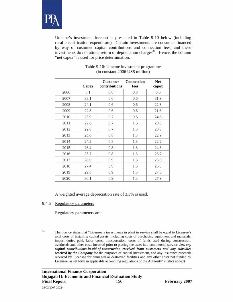
International Finance Corporation Bujagali II: Economic and Financial Evaluation Study Final Report 156 February 2007 26/02/2007-20224
Umeme’s investment forecast is presented in Table 9-10 below (including rural electrification expenditure). Certain investments are consumer-financed by way of customer capital contributions and connection fees, and these investments do not attract return or depreciation charges34. Hence, the column “net capex” is used for price determination.
Table 9-10: Umeme investment programme (in constant 2006 US$ million)
Capex Customer
contributionsConnection
fees Net
capex 2006 8.1 0.8 0.8 6.6 2007 33.1 0.6 0.6 31.9 2008 24.1 0.6 0.6 22.8 2009 22.8 0.6 0.6 21.6 2010 25.9 0.7 0.6 24.6 2011 22.8 0.7 1.3 20.8 2012 22.8 0.7 1.3 20.9 2013 25.0 0.8 1.3 22.9 2014 24.2 0.8 1.3 22.2 2015 26.4 0.8 1.3 24.3 2016 25.7 0.8 1.3 23.7 2017 28.0 0.9 1.3 25.8 2018 27.4 0.9 1.3 25.3 2019 29.8 0.9 1.3 27.6 2020 30.1 0.9 1.3 27.9
A weighted average depreciation rate of 3.3% is used.
9.4.6 Regulatory parameters
Regulatory parameters are:
34 The licence states that ”Licensee’s investments in plant in service shall be equal to Licensee’s total costs of installing capital assets, including costs of purchasing equipment and materials, import duties paid, labor costs, transportation, costs of funds used during construction, overheads and other costs incurred prior to placing the asset into commercial service, less any capital contributions-in-aid-of-construction received from customers and any subsidies received by the Company for the purposes of capital investment, and any insurance proceeds received by Licensee for damaged or destroyed facilities and any other costs not funded by Licensee, as set forth in applicable accounting regulations of the Authority” (italics added)
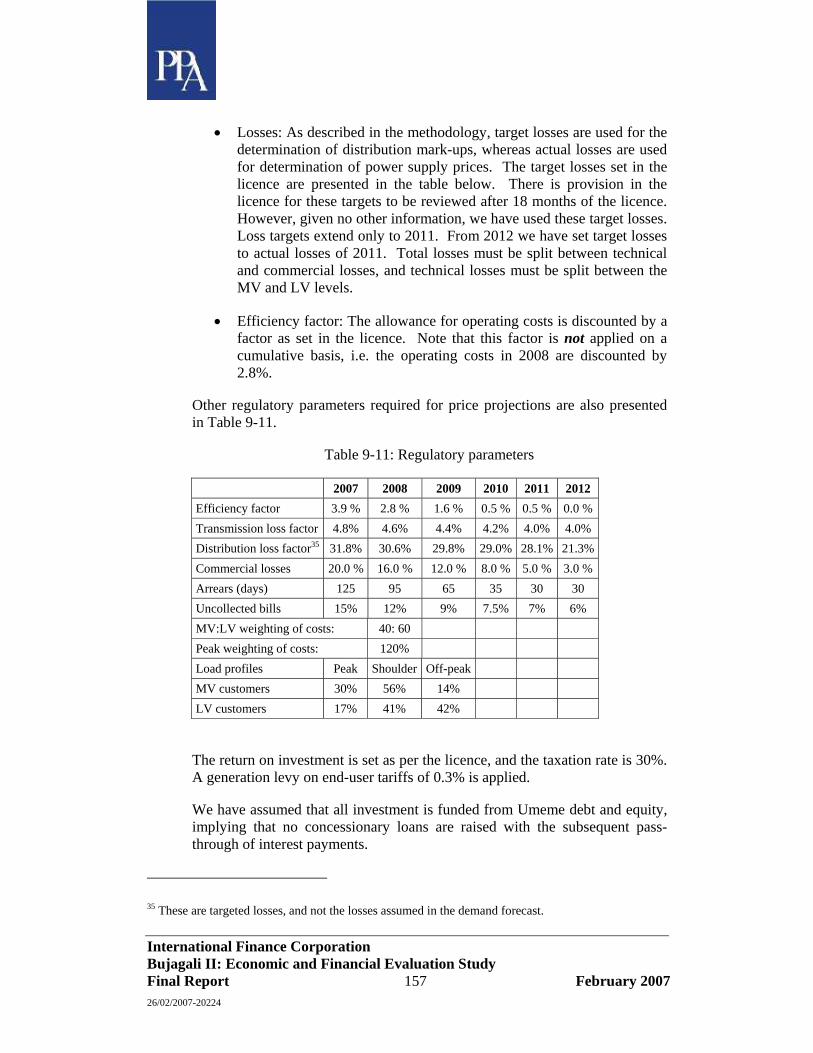
International Finance Corporation Bujagali II: Economic and Financial Evaluation Study Final Report 157 February 2007 26/02/2007-20224
• Losses: As described in the methodology, target losses are used for the determination of distribution mark-ups, whereas actual losses are used for determination of power supply prices. The target losses set in the licence are presented in the table below. There is provision in the licence for these targets to be reviewed after 18 months of the licence. However, given no other information, we have used these target losses. Loss targets extend only to 2011. From 2012 we have set target losses to actual losses of 2011. Total losses must be split between technical and commercial losses, and technical losses must be split between the MV and LV levels.
• Efficiency factor: The allowance for operating costs is discounted by a factor as set in the licence. Note that this factor is not applied on a cumulative basis, i.e. the operating costs in 2008 are discounted by 2.8%.
Other regulatory parameters required for price projections are also presented in Table 9-11.
Table 9-11: Regulatory parameters
2007 2008 2009 2010 2011 2012 Efficiency factor 3.9 % 2.8 % 1.6 % 0.5 % 0.5 % 0.0 % Transmission loss factor 4.8% 4.6% 4.4% 4.2% 4.0% 4.0% Distribution loss factor35 31.8% 30.6% 29.8% 29.0% 28.1% 21.3% Commercial losses 20.0 % 16.0 % 12.0 % 8.0 % 5.0 % 3.0 % Arrears (days) 125 95 65 35 30 30 Uncollected bills 15% 12% 9% 7.5% 7% 6% MV:LV weighting of costs: 40: 60 Peak weighting of costs: 120% Load profiles Peak Shoulder Off-peak MV customers 30% 56% 14% LV customers 17% 41% 42%
The return on investment is set as per the licence, and the taxation rate is 30%. A generation levy on end-user tariffs of 0.3% is applied.
We have assumed that all investment is funded from Umeme debt and equity, implying that no concessionary loans are raised with the subsequent pass-through of interest payments.
35 These are targeted losses, and not the losses assumed in the demand forecast.

International Finance Corporation Bujagali II: Economic and Financial Evaluation Study Final Report 158 February 2007 26/02/2007-20224
9.5 Results
9.5.1 Revenue requirements in the electricity sector
Figure 9-2 presents the total costs (or revenue requirements) in the electricity sector, broken down by each major component of the value chain. The revenue requirements increase substantially in 2008 as more thermal capacity comes on line, but then decrease somewhat as the balance of thermal production shifts from AGO to small-scale renewable plant and the cheaper HFO. In 2011, most of the thermal production (and costs) are substituted by Bujagali. Thereafter, costs are reasonably stable until new thermal production is required, adding to total costs. From 2017 onwards, Karuma displaces thermal production (although costs relating to the geothermal plant remain), leading to an increase in total costs. Network costs (including both transmission and distribution costs) steadily increase by approximately 7.5% per annum – a slightly slower rate of increase than in sales (8.5% per annum over the entire period to 2020).
Figure 9-2: Total revenue requirements in the electricity sector (in constant 2006 US$ million)
-
100
200
300
400
500
600
2007 2008 2009 2010 2011 2012 2013 2014 2015 2016 2017 2018 2019 2020
2006
US$
mill
ion
Bad debtsUmemeUETCLEmbedded renewablesThermalKarumaBujagaliEskom
9.5.2 Comparing costs of supply with assumed tariffs
Table 9-12 below presents the resulting tariff structures up to 2012 and compares them with the assumed values. In the period up to 2008, the assumed tariffs are below the calculated tariffs – largely due to the high costs of thermal generation. Over the period 2009-2012, the assumed tariffs and the calculated tariffs are close, although it is possible that tariffs could come down faster than assumed.

International Finance Corporation Bujagali II: Economic and Financial Evaluation Study Final Report 159 February 2007 26/02/2007-20224
Table 9-12: Comparing calculated tariffs with assumed tariffs (in constant 2006 US¢/kWh)
Domestic Commercial Industrial Average tariffs Assumed Calc’d Assumed Calc’d Assumed Calc’d Assumed Calc’d2007 23.3 31.0 20.5 31.0 9.4 18.5 17.6 26.7 2008 26.8 31.6 23.5 31.6 10.9 18.1 20.3 25.4 2009 26.8 25.5 23.5 25.5 10.9 13.8 20.3 19.7 2010 26.8 22.7 23.5 22.7 10.9 12.3 20.3 17.2 2011 22.8 18.0 20.0 18.0 9.2 8.8 17.2 14.9 2012 22.8 19.5 20.0 19.5 9.2 10.4 17.2 15.8
The fact that the assumed tariffs are below the actual costs of supply in the period to 2008 indicates that subsidies are required or tariffs need to be increased. The assumed tariff path in this period represents our view on the most viable phasing-in of the long-run cost-reflective tariff – that is, the tariffs in this period are transitional rather than intentionally cost-reflective.
If tariffs are to follow the assumed path, subsidies will be required in 2007 and 2008 only. The total subsidy requirement for these two years is estimated at US$ 148 million in nominal terms. The IDA credit to assist Uganda in overcoming the consequences of the emergency thermal programme should be more than sufficient to offset the estimated subsidy requirement. This indicates that the tariff path assumptions are reasonably consistent with current Government thinking in relation to power sector prices and sector support.
The analysis was continued beyond 2012 to examine the impact of additional capacity requirements in the expansion plan, including the tariff impact of the Karuma plant. Figure 9-3 compares the average cost with the assumed average tariff over the full period to 2020.
The results show that original tariff assumptions for the period 2009-2020 are slightly higher than the calculated average cost of supply. The analysis indicates that tariffs could come down faster than assumed from 2009 to 2011. After this point, the average tariff is approximately 1.2 US¢/kWh lower than the assumed constant tariff level of 17.2 US¢/kWh.

International Finance Corporation Bujagali II: Economic and Financial Evaluation Study Final Report 160 February 2007 26/02/2007-20224
Figure 9-3: Comparison of assumed tariffs with long-term average costs (in constant 2006 US¢/kWh)
-
5
10
15
20
25
30
2007 2008 2009 2010 2011 2012 2013 2014 2015 2016 2017 2018 2019 2020
2006
USc
/kW
h
Assumed tariff
Ave cost of supply
Tariff after available subsidies
Tariff in Jan 2007
Average cost of supply over this period is 16c/kWhcompared with an assumed tariff of 17.2c/kWh
High costs due to short-term thermal supplies
Available subsidies of $243m applied from 2007 to 2010 will reduce tariffs to around 17c/kWh
9.4.7 Impact of lower tariffs on demand forecast
While the ToR only requires a revision to the demand forecast if costs are determined as higher than the tariffs assumed, we have nonetheless examined the impact of revised tariff assumptions for the period from 2012 onwards.
If tariffs are reduced from 2009 in accordance with the projected average costs, this will exert an upward pressure on demand. The result (in the base case) is to increase generation requirements by 20 MW and 110 GWh in 2015 compared to the demand forecast used in this study (a 4% increase in requirements in 2015). This change is well within the low/high range considered in sensitivity analysis as shown in Figure 9-4 below. The increase in generation requirements may have the effect of scheduling new investment slightly earlier than expected, but is very unlikely to change the choice of least-cost expansion plan, or to have a significant impact on the cost of supply.
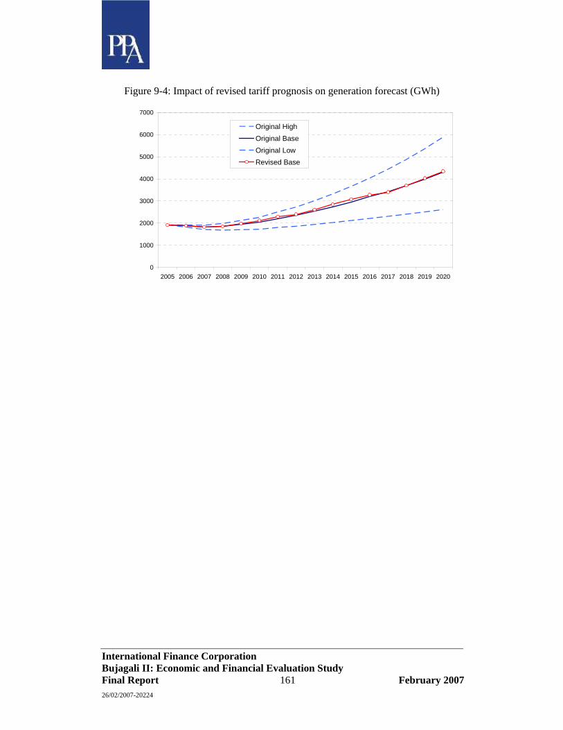
International Finance Corporation Bujagali II: Economic and Financial Evaluation Study Final Report 161 February 2007 26/02/2007-20224
Figure 9-4: Impact of revised tariff prognosis on generation forecast (GWh)
0
1000
2000
3000
4000
5000
6000
7000
2005 2006 2007 2008 2009 2010 2011 2012 2013 2014 2015 2016 2017 2018 2019 2020
Original HighOriginal BaseOriginal LowRevised Base

International Finance Corporation Bujagali II: Economic and Financial Evaluation Study Final Report 162 February 2007 26/02/2007-20224
10 Macro-economic Analysis
10.1 Summary
In order to determine the macro-economic impact of Bujagali on Uganda, two cases have been compared, assuming base demand forecast, base fuel and capital cost and low hydrology:
• The least cost expansion plan with Bujagali (‘with Bujagali’): this has Bujagali commissioned in 2011, some thermal and geothermal some few years later, and Karuma in 2017;
• The least-cost expansion plan without Bujagali (‘without Bujagali’): this has the Karuma plant commissioned as soon as possible (in 2012) and additional thermal and geothermal from 2014.
In relation to macro-economic impact, the main differences between the two cases are:
• The ‘with Bujagali’ case will imply that effects on investments and phasing out of thermal generation will happen one year earlier;
• The ‘with Bujagali’ case will have two major investments during the study period (Bujagali plus Karuma), whereas the ‘without Bujagali’ case has only one (Karuma);
• Relative to the ‘without Bujagali’ case, there will be very little thermal generation in the ‘with Bujagali’ case, up to 2020; and
• With the main set of assumptions (low hydrology and base demand forecast), the cost of energy will be lower in the ‘with Bujagali’ case.
In addition to putting an end to load shedding (in both cases but a year later in the ‘without Bujagali’ case), the main effects will be through power sector investments which will add a maximum of 0.3 percent to GDP in 2009 in both cases, with a similar reduction over time. In the longer term, the ‘with Bujagali’ expansion plan will afford 5 percent lower electricity tariffs than the ‘without Bujagali’ plan.
We assume that most investments in the power sector will made by the private sector and that these entities will be financed either by direct investments from abroad or by international borrowing. An exception may be UETCL which is Government owned and may therefore finance transmission systems investments related to hydro power projects by recourse to international borrowing.

International Finance Corporation Bujagali II: Economic and Financial Evaluation Study Final Report 163 February 2007 26/02/2007-20224
As there are no modelling tools that include behavioural relationships for the Ugandan economy available (see Section 10.2.1), the direct impacts will be discussed and put into perspective, but the total impact of the difference between the two cases on the future economic growth, balance of payments, and public finance in Uganda cannot be quantified with precision. However, the main conclusion is that the overall impact of the Bujagali project on the economy will be positive.
10.2 Macro-economic Parameters
10.2.1 Availability of Modelling Tools
The Consultant held meetings in Uganda with various institutions on issues related to macroeconomic effects of various scenarios for the supply of electricity. It was found that the tools available for analyzing the impact of power sector investments and production on other sectors are not well developed. Forecasts presented by international institutions and the GoU for the Ugandan economy are based on extrapolations and simple accounting formulae. There are no models with relationships representing the responses of various sectors to changes in income and prices.
There is an ongoing project at the Uganda Bureau of Statistics that will produce input/output tables for the Ugandan economy. A draft of the results was delivered to the Uganda Bureau of Statistics (UBOS) in February, but the results have not been made available to the Consultant.
10.2.2 Developments up to 2011 – the starting point
The base demand forecast uses the IMF forecasts for GDP as a reference scenario. The IMF has informed us that their forecast does not include the effects of the start up of any hydroelectric power plants or any other major power plants not yet commissioned.
As a basis for calculating ratios relative to GDP or its components beyond the period covered by the IMF forecast, we have produced a forecast for GDP to 2020 by keeping the growth rates in the IMF forecast constant at the final year (2010/11) values.
10.3 Effects on GDP Components
10.3.1 Household consumption
Electricity consumption makes up 1.2 percent of total household consumer expenditure. Only a small fraction of households have generators, and less than 10 percent have access to grid electricity. On a macro level, changes to the supply of electricity have only minor direct effects on household consumption. Electricity is also an input to the business sector, and many businesses will be in position to pass on changes in energy costs to consumers.

International Finance Corporation Bujagali II: Economic and Financial Evaluation Study Final Report 164 February 2007 26/02/2007-20224
The ‘without Bujagali’ case will have 5 percent higher tariffs than the ‘with Bujagali’ case. The direct impact of this on households is small.
Electricity costs (from the grid) are comparable to 3 percent of the business sector’s value added (and less in terms of total costs). Even if one assumes full mark-up of energy costs in output prices, the assumed 5 percent difference in electricity tariffs between the two cases have little indirect impact on households caused by the business sector’s passing on electricity costs to consumers.
The cost of unserved energy is substantial until 2011, but low after that year in both cases. While the ending of load shedding is important for households, there is no significant difference in load-shedding between the scenarios.
10.3.2 General government consumption and investment
Although data on government expenditure on electricity are not available, we assume that changes to the supply of electricity will not have major direct effects on government expenditure. However, the government’s financial situation will also be affected through:
• its participation in investments in hydroelectric power stations and transmission networks;
• possible changes to government subsidies to the power sector; and
• effects on the tax base that may have effects on government taxes and expenditures.
We assume that the Government (through its ownership of UETCL) will finance the transmission systems related to the Bujagali and Karuma plants, but will not participate in the financing of the power plants.
In the Bujagali case, the Government will invest US$ 28 million for transmission lines for Bujagali and then US$ 78 million for Karuma, US$ 106 million in total. In the Karuma case, only the US$ 78 million relating to the Karuma power plant will be relevant.
The impacts on the Government’s financial position are discussed in Section 10.4.
10.3.3 Business investment
The level of investment will differ between the two cases due to differences in investments in the power sector itself and because differences in tariffs and load shedding affect the business sector’s return on assets.
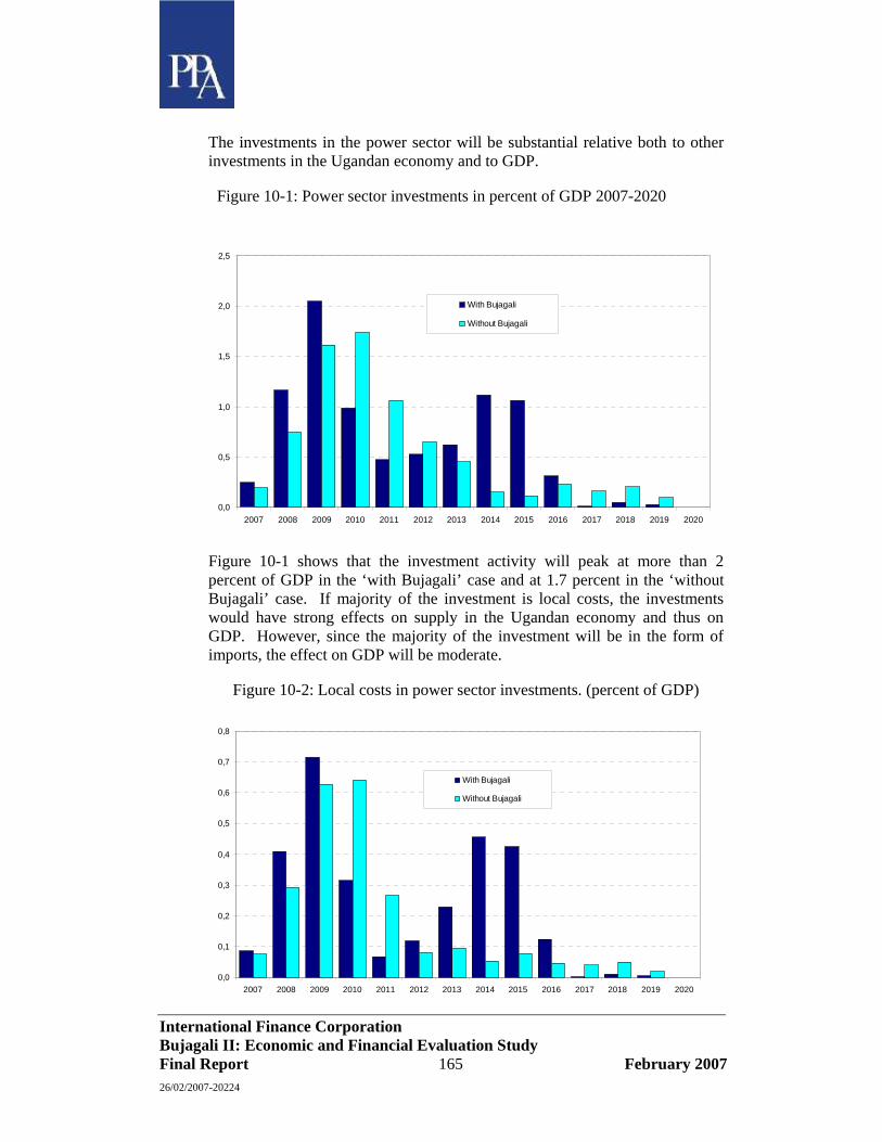
International Finance Corporation Bujagali II: Economic and Financial Evaluation Study Final Report 165 February 2007 26/02/2007-20224
The investments in the power sector will be substantial relative both to other investments in the Ugandan economy and to GDP.
Figure 10-1: Power sector investments in percent of GDP 2007-2020
0,0
0,5
1,0
1,5
2,0
2,5
2007 2008 2009 2010 2011 2012 2013 2014 2015 2016 2017 2018 2019 2020
With Bujagali
Without Bujagali
Figure 10-1 shows that the investment activity will peak at more than 2 percent of GDP in the ‘with Bujagali’ case and at 1.7 percent in the ‘without Bujagali’ case. If majority of the investment is local costs, the investments would have strong effects on supply in the Ugandan economy and thus on GDP. However, since the majority of the investment will be in the form of imports, the effect on GDP will be moderate.
Figure 10-2: Local costs in power sector investments. (percent of GDP)
0,0
0,1
0,2
0,3
0,4
0,5
0,6
0,7
0,8
2007 2008 2009 2010 2011 2012 2013 2014 2015 2016 2017 2018 2019 2020
With Bujagali
Without Bujagali
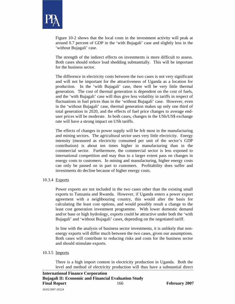
International Finance Corporation Bujagali II: Economic and Financial Evaluation Study Final Report 166 February 2007 26/02/2007-20224
Figure 10-2 shows that the local costs in the investment activity will peak at around 0.7 percent of GDP in the ‘with Bujagali’ case and slightly less in the ‘without Bujagali’ case.
The strength of the indirect effects on investments is more difficult to assess. Both cases should reduce load shedding substantially. This will be important for the business sector.
The difference in electricity costs between the two cases is not very significant and will not be important for the attractiveness of Uganda as a location for production. In the ‘with Bujagali’ case, there will be very little thermal generation. The cost of thermal generation is dependent on the cost of fuels, and the ‘with Bujagali’ case will thus give less volatility in tariffs in respect of fluctuations in fuel prices than in the ‘without Bujagali’ case. However, even in the ‘without Bujagali’ case, thermal generation makes up only one third of total generation in 2020, and the effects of fuel price changes to average end-user prices will be moderate. In both cases, changes in the USh/US$ exchange rate will have a strong impact on USh tariffs.
The effects of changes in power supply will be felt most in the manufacturing and mining sectors. The agricultural sector uses very little electricity. Energy intensity (measured as electricity consumed per unit of the sector’s GDP contribution) is about ten times higher in manufacturing than in the commercial sector. Furthermore, the commercial sector is less exposed to international competition and may thus to a larger extent pass on changes in energy costs to customers. In mining and manufacturing, higher energy costs can only be passed on in part to customers. Profitability does suffer and investments do decline because of higher energy costs.
10.3.4 Exports
Power exports are not included in the two cases other than the existing small exports to Tanzania and Rwanda. However, if Uganda enters a power export agreement with a neighbouring country, this would alter the basis for calculating the least cost options, and would possibly result a change to the least cost generation investment programme. With lower domestic demand and/or base or high hydrology, exports could be attractive under both the ‘with Bujagali’ and ‘without Bujagali’ cases, depending on the negotiated tariff.
In line with the analysis of business sector investments, it is unlikely that non-energy exports will differ much between the two cases, given our assumptions. Both cases will contribute to reducing risks and costs for the business sector and should stimulate exports.
10.3.5 Imports
There is a high import content in electricity production in Uganda. Both the level and method of electricity production will thus have a substantial direct
International Finance Corporation Bujagali II: Economic and Financial Evaluation Study Final Report 167 February 2007 26/02/2007-20224
effect on imports. Developments in the power sector will also affect imports indirectly through the level and composition of demand for non-energy goods and services.
Figure 10-3: Imports to power sector. (US$ million)
0
50
100
150
200
250
2006 2007 2008 2009 2010 2011 2012 2013 2014 2015 2016 2017 2018 2019 2020
With BujagaliWithout Bujagali
Figure 10-3 illustrates that the two cases will generate substantial imports to the power sector. The data do not include imports to serve self-generation of power and imports to other substitutes for unserved energy. From 2011, load shedding will be low in both cases. The total of imports to the power sector for the period from 2008 to 2020 will be US$ 1,397 million and US$ 1,656 million respectively in the ‘with Bujagali’ and ‘without Bujagali’ cases. The difference in imports is due to higher total costs in the ‘without Bujagali’ case, and somewhat higher imports content in thermal generation than in hydroelectric plants. In the ‘without Bujagali’ case, thermal generation will have to expand beyond 2020, which will stimulate imports.
The ‘with Bujagali’ case should provide for approximately 5 percent lower tariffs. Some of the savings on the spending on electricity will be used for imports.
10.3.6 Impacts on Balance of Payments and the Exchange Rate
We assume that all investments in power plants will be financed internationally through loans or equity. The initial inflow of capital will be serviced, appearing as a negative contribution to net income in the current account of the balance of payments.
We have calculated (the negative) contribution to net income (in the current account) by assuming that power sector investments will be financed with 75

International Finance Corporation Bujagali II: Economic and Financial Evaluation Study Final Report 168 February 2007 26/02/2007-20224
percent debt and 25 percent equity. Interest on debt is assumed to be 10 percent while return on equity is 17 percent after tax. Debt is repaid linearly over 20 years. The current account will also be directly affected by import to the power sector. The total direct impact on the current account is illustrated in Figure 10-4.
Figure 10-4: Identified Contributions to the current account of BOP
-300
-250
-200
-150
-100
-50
0
2006 2007 2008 2009 2010 2011 2012 2013 2014 2015 2016 2017 2018 2019
With Bujagali
Without Bujagali
In the ‘with Bujagali’ case, there will be two negative peaks in the direct contribution to the current account, related to the phased expenditure on investments in the two major hydro projects. In the ‘without Bujagali’ case, there will be only one negative peak. As an undiscounted sum over the 2006-2020 period, the identified negative impact on the current account is US$ 171 million higher in the “Without Bujagali” case.
The effects on the overall balance or the net use of reserves, also depends on the identified net inflow of capital related to the projects.
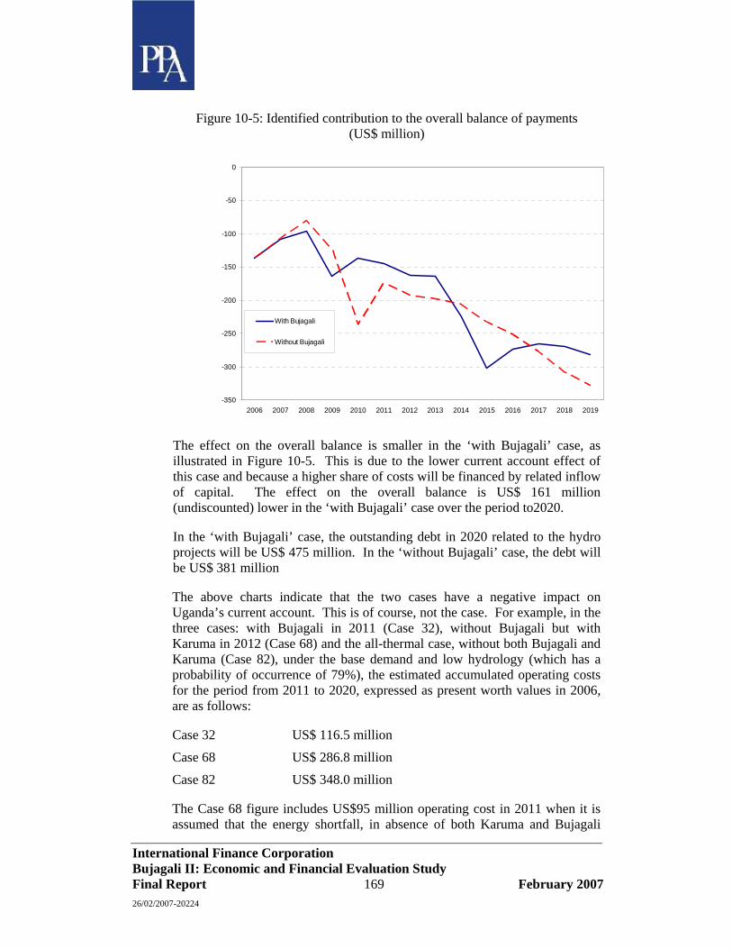
International Finance Corporation Bujagali II: Economic and Financial Evaluation Study Final Report 169 February 2007 26/02/2007-20224
Figure 10-5: Identified contribution to the overall balance of payments (US$ million)
-350
-300
-250
-200
-150
-100
-50
0
2006 2007 2008 2009 2010 2011 2012 2013 2014 2015 2016 2017 2018 2019
With Bujagali
Without Bujagali
The effect on the overall balance is smaller in the ‘with Bujagali’ case, as illustrated in Figure 10-5. This is due to the lower current account effect of this case and because a higher share of costs will be financed by related inflow of capital. The effect on the overall balance is US$ 161 million (undiscounted) lower in the ‘with Bujagali’ case over the period to2020.
In the ‘with Bujagali’ case, the outstanding debt in 2020 related to the hydro projects will be US$ 475 million. In the ‘without Bujagali’ case, the debt will be US$ 381 million
The above charts indicate that the two cases have a negative impact on Uganda’s current account. This is of course, not the case. For example, in the three cases: with Bujagali in 2011 (Case 32), without Bujagali but with Karuma in 2012 (Case 68) and the all-thermal case, without both Bujagali and Karuma (Case 82), under the base demand and low hydrology (which has a probability of occurrence of 79%), the estimated accumulated operating costs for the period from 2011 to 2020, expressed as present worth values in 2006, are as follows:
Case 32 US$ 116.5 million
Case 68 US$ 286.8 million
Case 82 US$ 348.0 million
The Case 68 figure includes US$95 million operating cost in 2011 when it is assumed that the energy shortfall, in absence of both Karuma and Bujagali

International Finance Corporation Bujagali II: Economic and Financial Evaluation Study Final Report 170 February 2007 26/02/2007-20224
would be met by the retention of the leased high speed diesel plant. Thus, the ‘with Bujagali’ case shows substantial savings in operating costs over the 2011 to 2020 period. Since the operating costs are dominated by fuel, the ‘with Bujagali’ option should lead to substantial reductions in expensive imported fuel over the other two options.
The above analysis does not take into account the positive impact of the improving reliability of the power supply and reduced reliance on expensive thermal generation. This will reduce both imports costs and total costs of energy in Uganda and will contribute to improved macro-economic conditions for Ugandan exporters. Both cases should thus over time contribute to improving Uganda’s current account in the balance of payments.
In the period up to 2020, there is not a large difference in the cumulative effect between the two cases. However, while the ‘without Bujagali’ case will require increasing imports of fuel for thermal generation after 2020, the ‘with Bujagali’ case will be associated with a downward trend in interest payments and thus appears more favourable than ‘without Bujagali’ after 2020.
In the investment period(s), imports will rise in both cases, and the deficit on the trade balance will increase. The investments will be linked to external financing covering both imported and local costs (except for transmission lines). External financing will be in excess of the imports for the investments, and the direct effect of the investments projects on net foreign reserves will thus be positive. The main reason why the accumulated negative effect on the overall balance of payments by 2019 is less than the effect on the current account is that there will still be substantial outstanding debt related to the project at this point in time. Looking further ahead, the effect on the overall balance of payments will be higher than the effect on the current account. In 2020, project related debt outstanding is estimated at US$ 475 million ‘with Bujagali’ and US$ 381 million ‘without Bujagali’. The debt is higher ‘with Bujagali’ due to the impact of Karuma commissioning in 2017.
The two cases will contribute to reducing other imports when the new power plants start producing. In our opinion, both cases should thus contribute to strengthening Uganda’s foreign exchange reserves. This could in turn contribute to strengthening the USh, but the direct effects are rather small both in absolute terms, and in terms of the differences between the two cases, relative to the size of the economy.
For the exchange rate, the prospect of improving the security of energy supplies is probably the most important factor. Both cases will improve confidence in the reliability of grid electricity supply in Uganda for many years to come. This should boost investors’ confidence and possibly contribute to a strengthening of USh if monetary policies do not offset this effect through the lowering of interest rates or interventions in the exchange market.

International Finance Corporation Bujagali II: Economic and Financial Evaluation Study Final Report 171 February 2007 26/02/2007-20224
10.4 Effects on the Government’s financial position
The developments in the energy sector will affect the Government’s financial position through five mechanisms:
• Excise duties on fuels,
• VAT on electricity sales,
• Indirectly through the general tax base (economic growth),
• The Government’s participation in the financing of transmission lines, and
• The Government subsidy on electricity generation (pre-Bujagali/Karuma).
The cases are based on the assumption that fuels for thermal generation will be exempted from taxes in whole forecast period. It is understood that the Ugandan authorities have not taken a decision on fuel tax exemptions, in the medium term. The assumption is therefore uncertain. If there will be excise duties on fuels for thermal generation after 2011, this will contribute to increased Government revenue in the ‘without Bujagali’ case, provided that these additional revenues are recovered from higher tariffs and not higher power sector subsidies.
The present VAT rate is 17 percent. On the basis of the forecast revenue requirement, illustrated in Figure 9-2, the annual Government revenue from VAT on electricity will be in the range of US$ 45 million in the 2007-2011 period, then increase gradually to US$ 94 million by 2020. In the ‘without Bujagali’ case, the revenue requirement for the electricity sector will be approximately 5% higher than shown in Figure 9-2, as will the Governments revenue from VAT on electricity. The difference in government revenue amounts to US$ 2.5-4.5 million per annum.
The Government will finance transmission lines through UETCL. In the ‘with Bujagali’ case, the Government will invest a total of US$ 106 million in transmission lines, while in the ‘without Bujagali’ case, the investment will be US$ 78 million. The Government will get a return on these investments. In the budget for 2006/07, USh 99.4 bn (US$ 53.7 million) was allocated to an energy fund that will be use to finance government investments in transmission lines as well as other energy investment projects. The Government will recover the investment costs through tariffs. The investment in the ‘with Bujagali’ case equates to approximately 1 percent of annual GDP and this will be spread over two 4-year periods, i.e. four years for Bujagali and four years for Karuma.
The Government will through its ownership of UECTL carry substantial risks related to the power sector through UECTL’s payment obligations under the

International Finance Corporation Bujagali II: Economic and Financial Evaluation Study Final Report 172 February 2007 26/02/2007-20224
power purchase agreements. However, we assume that the Government will not have to subsidise electricity after 2010 in the Bujagali case and after 2011 in the ‘without Bujagali’ case.